Embed Size (px)
Citation preview

HAL Id: hal-01005290https://hal.archives-ouvertes.fr/hal-01005290
Submitted on 15 Oct 2016
HAL is a multi-disciplinary open accessarchive for the deposit and dissemination of sci-entific research documents, whether they are pub-lished or not. The documents may come fromteaching and research institutions in France orabroad, or from public or private research centers.
L’archive ouverte pluridisciplinaire HAL, estdestinée au dépôt et à la diffusion de documentsscientifiques de niveau recherche, publiés ou non,émanant des établissements d’enseignement et derecherche français ou étrangers, des laboratoirespublics ou privés.
Distributed under a Creative Commons Attribution| 4.0 International License
Bending and buckling of inflatable beams : some newtheoretical results
Anh Le Van, Christian Wielgosz
To cite this version:Anh Le Van, Christian Wielgosz. Bending and buckling of inflatable beams : some new theoreticalresults. Thin-Walled Structures, Elsevier, 2005, 43 (8), pp.1166-1187. �10.1016/j.tws.2005.03.005�.�hal-01005290�

Bending and buckling of inflatable beams: Some new
theoretical results
A. Le van, C. Wielgosz
Faculty of Sciences of Nantes, GeM Institute of Research in Civil and Mechanical Engineering,
2, rue de la Houssiniere, BP 92208, Nantes 44322 cedex 3, France
The non linear and linearized equations are derived for the in plane stretching and bending of
thin walled cylindrical beams made of a membrane and inflated by an internal pressure. The
Timoshenko beam model combined with the finite rotation kinematics enables one to correctly
account for the shear effect and all the non linear terms in the governing equations. The linearization
is carried out around a pre stressed reference configuration which has to be defined as opposed to the
so called natural state. Two examples are then investigated: the bending and the buckling of a
cantilever beam. Their analytical solutions show that the inflation has the effect of increasing the
material properties in the beam solution. This solution is compared with the three dimensional finite
element analysis, as well as the so called wrinkling pressure for the bent beam and the crushing force
for the buckled beam. New theoretical and numerical results on the buckling of inflatable beams are
displayed.
Keywords: Inflatable beam; Thin walled beam; Membrane structure; Follower force; Bending; Buckling
1. Introduction
There are only a few papers dealing with theoretical studies on inflatable beams and it
seems that this research subject has been neglected in the last years. The first paper by
Comer and Levy [1] was published about 40-years-ago and its aim was to prove that
1
inflatable beams can be considered as usual Euler Bernoulli beams. At the same time,
Fichter [2] published a very interesting paper in which deflection of inflatable beams is
obtained by means of the principle of the total potential energy minimum. By taking into
account large displacements and following forces, Fichter has successfully included the
internal pressure in the equilibrium equations for inflatable beams subjected to bending
and compressive loads. Main et al. [3] realized experiments on cantilever inflatable beams
and made use of Comer and Levy’s theory. The pressure range considered in their
experiments was not significant enough to reveal the influence of the inflation pressure,
and their conclusion was that the usual Euler Bernoulli beam theory introduced by Comer
and Levy can be applied. However, as shown in [4,5], a usual beam theory cannot be used
to estimate the deflection of inflatable beams, because the inflation pressure does not
appear in the expression for the deflection.
In two recent papers, dealing with the mechanics of inflatable beams, one of the authors
has shown that the pressure effects should be involved in the final deflection, thus
reinforces Fichter’s solution. Deflections of flat panels [4] and tubes [5] have been
obtained under the following assumptions: the equilibrium equations should be written in
the deformed configuration in order to take into account the follower loads; Timoshenko’s
theory should be used to describe the kinematics of the beam (see Fig. 5 in [4] and Fig. 2 in
[5]). Beam analytical and finite element solutions [6] were obtained to give the sought
deflection. In every case, comparisons between theoretical solutions and experimental
results for simply supported inflated beams with various boundary conditions have shown
a very good agreement.
In the present work, a new formulation for inflatable beams is proposed in order to
improve Fichter’s theory. The non-linear equations for the in-plane stretching and bending
of an inflated beam are derived from the Lagrangian form of the virtual work principle.
One additional assumption compared with Fichter’s ones is introduced: the finite rotation
kinematics, which is shown to enable one to correctly account for all the non-linear terms
in the governing equations. Subsequently, the whole equation set is linearized around a
pre-stressed reference configuration which has to be defined as opposed to the so-called
natural state. Two examples are then investigated: the bending and the buckling of a
cantilever beam. Their analytical solutions show that the inflation has the effect of
‘increasing the material properties.’ The numerical results are compared with the
membrane finite element ones obtained within the three-dimensional framework.
Eventually, discussion of the validity of the solutions exhibits the notions of the wrinkling
pressure for the bent beam and the crushing force for the buckled beam. To the authors’
knowledge, the results on the buckling of inflatable beams are novel.
2. Governing equations
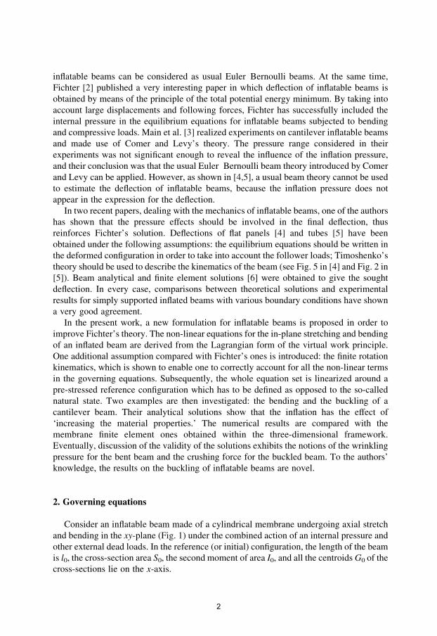
Consider an inflatable beam made of a cylindrical membrane undergoing axial stretch
and bending in the xy-plane (Fig. 1) under the combined action of an internal pressure and
other external dead loads. In the reference (or initial) configuration, the length of the beam
is l0, the cross-section area S0, the second moment of area I0, and all the centroids G0 of the
cross-sections lie on the x-axis.
2

Fig. 1. The inflated beam model.
In order to derive the governing equations for the inflatable beam, use will be made of
the principle of virtual work in the three-dimensional Lagrangian form
c virtual displacement field V�;
ðU0
PT : grad V� dU0 C
ðU0
f0$V� dU0
C
ðvU0
V�$P$N dS0 0 ð1Þ
where U0 is the region occupied by the body in the reference configuration, vU0 its
boundary, P the first Piola Kirchhoff stress tensor, f0 the body force per unit reference
volume and N the unit outward normal in the reference configuration.
2.1. Displacement and strain fields
Let us denote by U(X) (U(X), V(X), 0), the displacement of the centroid of a current
cross-section at abscissa X (all the components are related to the base (x,y,z)). We assume
that during the deformation the cross-section remains plane, but not perpendicular to the
bent axis of the beam (Timoshenko beam model). Then, by denoting q(X) the finite
rotation of the cross-section, the displacement of any material point P0(X,Y,Z) is given by:
UðP0Þ
U
V
0
C
cos q 1 sin q 0
sin q cos q 1 0
0 0 0
264
375
0
Y
Z
8><>:
9>=>;
U Y sin q
V Yð1 cos qÞ
0
�������
�������(2)
One readily deduces the components of the Green strain tensor from (2):
EXX U;x Y cos qq;x C1
2½U2
;x CV2;x CY2q2
;x 2YU;x cos qq;x
2YV;x sin qq;x�
EXY
1
2½V;x cos q ð1 CU;xÞsin q� EYY 0
(3)
The axial strain EXX involves linear and quadratic terms in Y, whereas the shear
component EXY does not depend on Y and is constant over the cross-section.
3

2.2. Virtual displacement field
Let us denote by V*(X) (U*(X),V*(X),0), the virtual displacement of the centroid of a
current cross-section. The following expression is chosen for the virtual displacement of a
current material point P0
V�ðP0Þ V� CU� !GP (4)
where U*(X) (0,0,q*(X)) is the virtual rotation. Note that Relation (4) involves the final
vector GP, not the initial vector G0P0, as in the real velocity field in mechanics of rigid
bodies. Since vector GP in turn can be expressed in terms of Lagrangian variables by using
the rotation operation: GP ( Y sin q,Y cos q,Z), it comes from (4):
V�ðP0Þ
�����U� Y cos qq�
V� Y sin qq�
0
(5)
Thus, the virtual displacement field is completely defined by three scalar functions
U*(X), V*(X) and q*(X).
2.3. Stresses
The matrix of the second Piola Kirchhoff (symmetric) stress tensor S in the base
(x,y,z) is assumed to take the following form:
½S�
SXX SXY 0
SXY 0 0
0 0 0
264
375 (6)
The material is assumed to be hyperelastic isotropic, obeying the Saint Venant
Kirchhoff constitutive law, characterized by the Young modulus E, the Poisson ratio n and
the initial (or residual) stresses S0XX , S0
XY induced by the preliminary inflation of the beam:
SXX S0XX CE$EXX SXY S0
XY C2G$EXY GE
2ð1 CnÞ
� �(7)
In the sequel, it is convenient to introduce the following generalized stresses
N
ðS0
SXX dS0 T
ðS0
SXY dS0 M
ðS0
YSXX dS0 (8)
which represent the (material) axial force, the shear force and the bending moment acting
on the reference cross-section S0. By assuming that the cross-section is symmetrical with
respect to the G0z-axis so thatÐ
S0Y dS0 0 and
ÐS0
Y3 dS0 0, one gets the expressions
4

for the generalized stresses in terms of the displacements from (3), (7) and (8):
N N0 CES0 U;X C1
2U2
;X C1
2V2;X C
I0
2S0
q2;X
� �
T T0 CGS0ðV;X cos q ð1 CU;XÞsin qÞ
M M0 CEI0ðð1 CU;XÞcos q CV ;X;X ;Xsin qÞq;X
(9)
In the above, N0, T0 and M0 are the resultants of the initial stresses on the cross-section.
As is seen later, very often simplifying assumptions on S0XX , S0
XY lead to T0 M0 0.
Furthermore, in practice the coefficient GS0 in (9) is replaced by kGS0, where the so-called
correction shear coefficient k is determined from the shape of the cross-section. The value
usually found in the literature (see, e.g. Ref. [7]) for circular thin tubes is k 0.5.
2.4. Virtual stress work
From the relation between the first and second Piola Kirchhoff stresses P FS (F is
the deformation gradient) and the definitions (8), we obtain the expression for the internal
virtual work:
ðU0
PT : grad V� dU0
ðI0
0½ðNð1 CU;xÞCM cos qq;x T sin qÞ�U�
;X C ½ðNV;x CM sin qq;x
CT cos qÞ�V�;X C ½Mð ð1 CU;xÞsin qq;x CV;x cos qq;xÞ Tðð1
CU;xÞcos q CV;x sin qÞ�q�
C Mðð1 CU;xÞcos q CV;x sin qÞC
ðS0
Y2S;XX dS0q;x
264
375q�;x dX (10)
The integralÐ
S0Y2S;XX dS0 in (10) can be recast as follows, assuming that the initial
stress S0XX takes the following form general enough in practical purposes: S0
XX a0Cb0Y Cg0Y2 and that S0
XY does not depend on Y. Hence, from (3a) and (7a) SXX is of the
form SXX aCbY CgY2, where g g0C ð1=2ÞEq2;x. Substituting this into definition (8)
gives
N
ðS0
SXX dS0 aS0 CgI0 M
ðS0
ySXX dS0 bI0 (11)
5

which entails
SXX
N
S0
gI0
S0
M
I0
Y CgY2
and thenðS0
Y2S;XX dS0
NI0
S0
Cg
ðS0
Y4dS0
I20
S0
0B@
1CA NI0
S0
C1
2KEq2
;x CKg0 (12)
where
K
ðS0
Y4 dS0
I20
S0
is a quantity depending on the initial geometry of the cross-section, like S0 and I0. This
quantity is involved in the non-linear equations of the problem; however, it will be seen
that it disappears in the linearized theory.
2.5. External virtual work due to dead loads
The Lagrangian expression for the external virtual work due to dead loads is:
W�ext
ðU0
f0ðP0Þ$V�ðP0Þ dU0 C
ðvU0
V�ðP0Þ$PðP0Þ$NðP0Þ dS0 (13)
Since the handling of dead load work is standard, it will not be detailed here. Let us just
give its final Eulerian expression in the case of the beam:
W�ext
ðl
0ðpxU� CpyV� Cmq�Þdx CXð0ÞU�ð0ÞCYð0ÞV�ð0ÞCGð0Þq�ð0Þ
CXðIÞU�ðIÞCYðIÞV�ðIÞCGðIÞq�ðIÞ (14)
In the above, l is the current length, (px, py) are the in-plane components of the dead
load per unit length, m the moment per unit length, (X($), Y($)) designates the components
of the resultant force at end sections x 0 or l, G the resultant moment. All these loads are
applied in the current configuration. It should be mentioned that expression (14) is
obtained since vector GP is involved in the virtual displacement (4) instead of G0P0.
2.6. External virtual work due to the internal pressure
Before external dead loads are applied, the beam is inflated by an internal pressure p$n
(where n is the outward unit normal in the current configuration) which gives the beam its
bearing capacity.
The contribution of the internal pressure will be determined under the assumption that the
reference volume U0 is a circular cylinder of radius R0. This assumption, combined with the
Timoshenko kinematics (2), implies that any cross-section remains a circular disk of radius R0
6

during the deformation. This means that the change in shape (ovalization or warping) of the
cross-section is not taken into account, as is the case of all usual beam models.
The virtual work of the pressure is computed by adding the works on the cylindrical
surface and on both ends.
2.6.1. Integral over the cylindrical surface
Let us represent the reference cylindrical surface by curvilinear coordinates (x1,x2)
(R04, X), where 4 is the polar angle between the normal n at the point x with the y-axis.
According to the displacement field (2), the current element surface is:
n dSvx
vx1
vx
vx2
dx1dx2�����cos 4ðV;X R0 cos 4 sin qq;XÞ
cos 4ð1 CU;X R0 cos 4 cos qq;XÞ
sin 4ðsin qV;X R0 cos 4q;X Ccosqð1 CU;XÞÞ
dx1dx2 (15)
The virtual displacement field (5) can be recast as:
V�ðP0Þ
�����U� R0 cos 4 cos qq�
V� R0 cos 4 sin qq�
0
(16)
From relations (15) and (16), one obtains the contribution of the pressure over the
cylindrical surface:ðCylindrical surface
V�ðP0Þ$n dS
pR20
ðl
0½U� sin qq;X V� cos qq;X Cq�ðcos qV;X sin qð1 CU;XÞÞ�dX (17)
The underlined terms stem from the finite rotation adopted in expression (2) for the
displacement field.
2.6.2. Integrals over the ends
These integrals are computed in the similar way as in the case of dead loads. For
instance, from relation (4) and the equality pn dS s$n dS on the end x l (s is the
Cauchy stress), we get:ðEnd xZI
V�ðP0Þ$pn dS
ðEnd xZI
sðPÞ$nðPÞ dS C
ðEnd xZI
GP!sðPÞ$nðPÞ dS$U� RV� CGU� (18)
7

Clearly, the torque G due to the pressure is zero on the ends. Moreover, by virtue of the
assumption that the reference volume U0 is a circular cylinder of radius R0, the resultant
force is R ppR20n. Hence:ð
End xZl
V�ðP0Þ$pn dS ppR20ðU
� cos q CV� sin qÞ (19)
2.6.3. Virtual work of the pressure
W�pressure P
ðI0
0½U� sin qq;X V� cos qq;X Cq�ðcos qV;X sin qð1 CU;XÞÞ�dX
CP½U� cos q CV� sin q�l00 ð20Þ
2.7. Equilibrium equations and boundary conditions
Integrating by parts the principle of virtual work (1) and using (10), (12), (14) and (20),
lead to the following equilibrium equations for the inflated beam
ðNð1CU;XÞÞ;X ðMcosqq;XÞ;X CðT sinqÞ;X Psinqq;X
pX
ðNV;XÞ;X ðM sinqq;XÞ;X ðT cosqÞ;X CPcosqq;X
pY
ðMð1CU;XÞÞ;X cosq ðMV;XÞ;X sinqCðð1CU;XÞcosqCV;X sinqÞT
NI0
S0
C1
2EKq2
;X CKg0
� �q;X
� �;X
PðcosqV;X sinqð1CU;XÞÞ m
(21)
together with the boundary conditions:
Nð0Þð1CU;Xð0ÞÞCMð0Þcosqð0Þq;Xð0Þ Tð0Þsinqð0Þ Pcosqð0Þ Xð0Þ (22a)
NðI0Þð1CU;XðI0ÞÞCMðl0ÞcosqðI0Þq;XðI0ÞCTðI0ÞsinqðI0Þ PcosqðI0Þ XðI0Þ
(22b)
Nð0ÞV;Xð0ÞCMð0Þsinqð0Þq;Xð0ÞCTð0Þcosqð0Þ Psinqð0Þ Yð0Þ (22c)
NðI0ÞV;XðI0ÞCMðl0ÞsinqðI0Þq;XðI0ÞCTðI0ÞcosqðI0Þ PsinqðI0Þ YðI0Þ (22d)
Mð0Þð1CU;Xð0ÞÞcosqð0ÞCMð0Þsinqð0ÞV;Xð0Þ
CNð0ÞI0
S0
C1
2EKq2
;Xð0ÞCKg0
� �q;Xð0Þ Gð0Þ (22e)
8

MðI0Þð1CU;XðI0ÞÞcosqðI0ÞCMðI0ÞsinqðI0ÞV;XðI0Þ
CNðI0ÞI0
S0
C1
2EKq2
;XðI0ÞCKg0
� �q;XðI0Þ GðI0Þ (22f)
It remains to substitute relations (9) for (N,M,T) in Eq. (21) to obtain a set of three non-
linear equations with three unknowns (U,V,q). Relations (21) (22f) are similar to those
obtained by Fichter [2], the additional terms are due to the fact that here the displacement
field (2) involves finite rotation.
3. Linearized equations
In this work, we shall confine ourselves to small deformations so as to deal with
linearized equations which are simpler to solve. The linearization of the equations will be
performed about the reference configuration which is in a pre-stressed state. For instance,
in the case of bending, the pre-stress is due to the preliminary inflation of the beam; in the
case of buckling, the pre-stress also includes the compressive load.
The linearization process is based on usual hypotheses on the magnitudes of the
displacements and the rotation:
(i) V/l0 and q are infinitesimal quantities of order 1,
(ii) U/l0 is infinitesimal of order 2.
Furthermore, the following assumptions are made on the initial stresses:
(i) The initial axial stress S0XX is constant over the cross-section. Thus, M0 g0 0.
(ii) The initial shear stress S0XY is zero. Thus, T0 0.
Taking these assumptions into account, one arrives at the linearized expressions for the
constitutive laws (9)
N N0 T kGS0ðV;x qÞ M EI0q;X (23)
From (21), the linearized equilibrium equations are:
N0;X pX
ðN0 CkGS0ÞV;X2 C ðP CkGS0Þq;X pY
E CN0
S0
� �I0q;X2 C ðP CkGS0ÞðV;X qÞ m
(24)
The linearized boundary conditions are derived from (22a) (22f):
N0ð0Þ P Xð0Þ (25a)
N0ðl0Þ P Xðl0Þ (25b)
9

ðN0ð0ÞCkGS0ÞV;Xð0Þ ðP CkGS0Þqð0Þ Yð0Þ (25c)
ðN0ðl0ÞCkGS0ÞV;Xðl0Þ ðP CkGS0Þqðl0Þ Yðl0Þ (25d)
E CN0ð0Þ
S0
� �I0q;Xð0Þ Gð0Þ (25e)
E CN0ðI0Þ
S0
� �I0q;XðI0Þ GðI0Þ (25f)
The linearized Eqs. (24) (25f) are quite similar to those obtained by Fichter [2]. Yet
there are two slight differences: (i) the linearization process, based on a well-defined
reference configuration, definitely shows that the obtained equations form a set of
linearized equations in terms of displacements U, V and rotation q; (ii) the pressure is
equally involved in the equilibrium equations and boundary conditions, so that it modifies
both the Young modulus and the shear modulus. This modification will be more explicit in
the bending and buckling examples considered in the next sections.
In addition, it should be mentioned that all the reference dimensions (e.g. length l0,
cross-section area S0 and second moment of area I0) are themselves functions of the
pressure p. Computing their values corresponding to a given pressure may be difficult, but
this is an independent subject which actually is common to every problem with a pre-
stressed reference configuration.
3.1. Solution scheme
Eq. (24) and the boundary conditions (25a) and (25b), related to the axial displacement
U, are decoupled from the rest and can easily be integrated. Let us describe how to solve
Eq. (24) and the boundary conditions (25c) (25f), related to the deflection V and the
rotation q.
Eq. (24) can be used to eliminate V,X as
V;X
ðP CkGS0Þ
ðN0 CkGS0Þq
C
ðN0 CkGS0Þ(26)
where CÐ
pY dX denotes a primitive of the load pY. Inserting (26) into (24) provides a
differential equation of second order in q:
E CN0
S0
� �I0q;X2 C
ðP CkGS0Þ
ðN0 CkGS0ÞðP N0Þq m CC
ðP CkGS0Þ
ðN0 CkGS0Þ(27)
The above equation is similar to that obtained in [5]. Integrating it leads to three
constants of integration, whereas integrating (26) leads to one additional constant. These
four constants are determined by means of the boundary conditions (25c) (25f).
10

4. Bending of an inflatable beam
In this section, we consider, as the first example, the linearized problem of an inflated
cantilever beam under bending. The beam is made of a cylindrical membrane, its reference
length is l0, its reference radius R0 and its reference thickness h0. The beam is built-in at
end X 0, subjected to an internal pressure p and a transverse force Fy at end X l0.
4.1. Deflection and rotation
From the equilibrium Eq. (24) and the boundary conditions (25a) and (25b), one readily
gets the initial axial force N0(X) P. Hence, Eqs. (26) and (27) become:
V;X qC
P CkGS0
ðHere; C is a constant of integrationÞ (28)
E CP
S0
� �I0q;X2 C (29)
Taking into account the boundary conditions (25c) (25f)
Vð0Þ qð0Þ q;Xðl0Þ 0 (30)
ðP CkGS0ÞðV;Xðl0Þ qðl0ÞÞ F (31)
one obtains the deflection and the rotation along the beam:
VðxÞF
ðE CP=S0ÞI0
I0x2
2
x3
6
� �C
Fx
P CkGS0
(32)
qðxÞF
ðE CP=S0ÞI0
I0xx2
2
� �(33)
The solution is linear with respect to force F, yet non-linear with respect to the pressure.
First, the pressure appears in the denominators of the right-hand sides of (32) and (33).
Second, the reference dimensions l0, S0, and I0 themselves depend on the pressure;
however, further numerical results show that this dependence may not be too strong.
If the internal pressure is zero, these relations give the well-known results for the
Timoshenko beam model. However, contrary to a classical beam, here the inflatable beam
is made of a membrane, so the pressure cannot be equal to zero for the beam not to
collapse. This fact will be discussed below in connection with the validity of the solution.
The influence of the internal pressure on the beam response is clearly shown in the
previous relations: the inflation amounts to strengthen the Young modulus and the shear
modulus. In particular, when p tends to infinity, so do the equivalent material properties
and the deflection and the rotation are identically zero.
In a recent paper [5], a solution for the bending problem was obtained by using the force
formulation. The Taylor expansion of the deflection expression therein with respect to
11

the resultant pressure P shows that the first non-zero term in P is a quadratic term:
VðxÞF
EI0
1P2
ðkGS0Þ2
� �I0x2
2
x3
6
� �C
Fx
kGS0
(34)
On the other hand, the Taylor expansion of relation (32) shows that the first non-zero
terms in P are linear:
VðxÞF
EI0
1P
ES0
� �I0x2
2
x3
6
� �C
Fx
kGS0
1P
kGS0
� �(35)
Relations (34) and (35) show that whichever of the formulations is used to estimate the
deflection, one obtains the same leading terms which come from the beam and yarn
compliances. Not surprisingly, the additional terms are different due to the very
differences between the force and displacement formulations.
Eventually, it should be mentioned that the deflection of inflated panels obtained in [4]
is identical to (32), provided the Young modulus E in [4] is replaced by ECP/S0. Also,
studies in progress show that the finite element derived in [6] for inflatable panels is
identical to that for inflatable beams, when the same substitution is carried out.
4.2. Limit of validity of the solution
Of course, one has to check a posteriori that the deflection and the rotation given by (32)
and (33) satisfy the small deformation hypothesis required by the linearization process.
Yet there is another condition for the solution to hold: as mentioned above, since the
inflatable beam is made of a membrane, the internal pressure must be high enough. More
precisely, the solution is valid if the principal stresses at any point in the beam are non-
negative. One can check that this amounts to saying that the axial stress SXX at the point
(X 0,Y R0,Z 0) is non-negative:
SXX S0XX
M
I0
YpR0
2h0
FI0
pR30h0
R0 R0 4 F%pR3
0p
2I0
(36)
Recall that the reference length l0 and radius R0 are (increasing) functions of the
pressure p. Inequality (36) shows that given a force F, the internal pressure must be high
enough for the bending solution to be meaningful. There exists a lower bound for the
pressure, referred to as the wrinkling pressure of the beam, below which a wrinkle appears
first at the point (X 0,Y R0,Z 0) and the bending solution is no longer valid.
4.3. Comparison with 3D membrane finite element results
In order to assess the proposed theory, the numerical values of the deflection (32) will
be compared to three-dimensional membrane finite element results. The membrane
computations are carried out using a general purpose non-linear finite element program,
based on the total Lagrangian formulation. The beam is modelled as a three-dimensional
membrane structure; the membrane elements have zero bending stiffness and satisfy the
usual plane stress condition. The three-dimensional constitutive law is the Saint-Venant
12

Kirchhoff one, characterized by the Young modulus E and Poisson ratio n, or equivalently,
by the Lame constants (l, m).
Discretizing the virtual power principle by the finite element technique leads to a non-
linear equilibrium equation in terms of the displacement field, which is solved using the
Newton iterative scheme. The total tangent stiffness matrix is the sum of (i) the stiffness
due to the internal forces and (ii) the stiffness due to the pressure. As the matter is standard,
let us just make a brief reminder for the internal forces. By denoting NNE the node number
of an element, the element stiffness matrix due to the internal force writes
ci; j2½1; 3NNE�;Keij
ðelement
Na;aNb;b dpqSba Cxp;gxq;d
vSag
vEbd
� �h0 dS0 (37)
where x denotes the current position of a particle belonging to the reference middle surface
S0 of the membrane; Na, a2[1, NNE], are the shape functions used to define the geometry
as well as the displacement in each element (isoparametric element). All the derivations
are performed with respect to curvilinear coordinates defining the membrane element.
Here, integers a,b2[1, NNE] and p,q2{1,2,3} are related to indices i and j by i 3(a
1)Cp, j 3(b 1)Cq. Implicit summation is carried out over a,b,g,d, 2{1,2}.
Taking into account the plane stress condition S33 0, one readily gets the expression
for the tangent modulus
vSab
vEdg
mðGagGbd CGadGbgÞC2lm
2m ClGabGgd (38)
where Gab the contravariant components of the metric tensor defined on the reference
middle surface.
Also, the path-following and branch switching techniques are included in the numerical
scheme, in order to deal with possible limit and bifurcation points, as seen in the buckling
case below. For membrane structures, an artificial initial stress has to be added in the first
increment. It is, however, removed in the next increments.
It should be emphasized that in the 3D membrane finite element solution, the loading is
applied in two successive stages: first, the beam is inflated to a given pressure p, and then a
force F is applied. At the very beginning of the first stage, the internal pressure is zero and
the beam is in a natural (or stress free) state. On the other hand, the reference
configuration, which corresponds to the beginning of the second stage (before the force F
is applied), is in a pre-stressed state. To clearly distinguish between the two states, we use
index : to denote the quantities in the natural state, as opposed to the usual index o for
quantities related to the reference configuration. Thus, l:, R: and h: designate the
natural length, radius and thickness, respectively; while l0, R0 and h0 the reference
dimensions, which vary as functions of the pressure.
4.4. Numerical results
The numerical computations are performed with three values of natural radius R:,
three values of natural length l: and four values of pressure p, while other quantities
13

Table 1
Data set for numerical computations
Natural thickness, h: (m) 125!10K6
Young modulus, E (N/m2) 2.5!109
Poisson ratio, n 0.3
Correction shear coefficient, k 0.5
Natural radius, R: (m) 0.04 0.06 0.08
Natural length, l: (m) 0.65 0.90 1.15
Pressure, p (N/m2) 0.5!105 105 1.5!105 2!105
(the natural thickness h:, Young modulus E, Poisson ratio n and correction shear factor k)
remain fixed, as shown in Table 1.
As mentioned above, the correction shear coefficient k, introduced after expression (9)
for the shear force T, is taken equal to the usual value for circular thin tubes, i.e. k 0.5.
As the problem is linear with respect to force F, we take F 1N in all the numerical
computations. Fig. 2 shows a typical mesh used in 3D membrane finite element
computations, containing 2401 nodes and 768 eight-node quadrilaterals and six-node
triangles. The reference length l0, radius R0 and thickness h0 are computed as functions of
the internal pressure by using the well-known elastic small strain analytical solution for
thin tubes. For instance, the expression for the reference thickness is:
h0 h:
3n
E
pR:
2(39)
With the chosen natural radii and pressures, it is found that the reference thickness is
virtually identical to the natural thickness, to within 2% at most. In the case of more
complex geometries, one should use a membrane finite element solution for obtaining the
reference length l0 and radius R0, and an appropriate estimate for the reference thickness h0.
Table 2 and Fig. 3 give the maximum deflection in the cantilever given by (32) as a
function of the length of the beam and the internal pressure, in comparison with the
deflection obtained by 3D membrane finite elements. Given one fixed natural radius R:,
one natural length l:, there are in Table 2 four reference lengths l0, depending on whether
pressure p is 0.5!105, 105, 1.5!105 or 2!105pa, respectively.
Fig. 2. A typical mesh used in 3D membrane finite element computations.
14

Table 2
Maximum deflection in the cantilever given by the inflated beam theory, compared with the 3D finite element
results. All deflections are obtained with force FZ1N.
Natural
length,
l: (m)
Pressure
(N/m2)
Reference
length,
l0 (m)
Reference
radius,
R0 (m)
Reference
thickness,
h0 (m)
Deflection (m)
By the inflat-
able beam
theory
By the mem-
brane finite
element
Diff-
eren-
ce
(%)
Case 1. Natural radius R: Z0:04 m
0.65 5.0!104 6.508!10K1 4.022!10K21.246!10K4 1.481!10K3 1.487!10K3 K0.4
1.0!105 6.517
!10K1!10K014.044!10K2!10K02
1.243!10K4 1.462!10K3 1.461!10K3 0.1
1.5!105 6.525!10K1 4.065!10K21.239!10K4 1.443!10K3 1.436!10K3 0.5
2.0!105 6.533!10K1 4.087!10K21.236!10K4 1.425!10K3 1.413!10K3 0.9
0.9 5.0!104 9.012!10K1 4.022!10K21.246!10K4 3.877!10K3 3.886!10K3 K0.2
1.0!105 9.023!10K1 4.044!10K21.243!10K4 3.828!10K3 3.820!10K3 0.2
1.5!105 9.035!10K1 4.065!10K21.239!10K4 3.779!10K3 3.757!10K3 0.6
2.0!105 9.046!10K1 4.087!10K21.236!10K4 3.731!10K3 3.696!10K3 1.0
1.15 5.0!104 1.151 4.022!10K21.246!10K4 8.041!10K3 8.054!10K3 K0.2
1.0!105 1.153 4.044!10K21.243!10K4 7.939!10K3 7.920!10K3 0.2
1.5!105 1.154 4.065!10K21.239!10K4 7.838!10K3 7.791!10K3 0.6
2.0!105 1.156 4.087!10K21.236!10K4 7.740!10K3 7.665!10K3 1.0
Case 2 Natural radius R: Z0:06 m
0.65 5.0!104 6.512!10K1 6.049!10K21.245!10K4 4.514!10K4 4.554!10K4 K0.9
1.0!105 6.525!10K1 6.098!10K21.239!10K4 4.427!10K4 4.426!10K4 0.0
1.5!105 6.537!10K1 6.147!10K21.234!10K4 4.342!10K4 4.313!10K4 0.7
2.0!105 6.550!10K1 6.196!10K21.228!10K4 4.259!10K4 4.207!10K4 1.2
0.9 5.0!104 9.017!10K1 6.049!10K21.245!10K4 1.163!10K3 1.166!10K3 K0.3
1.0!105 9.035!10K1 6.098!10K21.239!10K4 1.141!10K3 1.136!10K3 0.4
1.5!105 9.052!10K1 6.147!10K21.234!10K4 1.119!10K3 1.108!10K3 1.0
2.0!105 9.069!10K1 6.196!10K21.228!10K4 1.098!10K3 1.081!10K3 1.5
1.15 5.0!104 1.152 6.049!10K21.245!10K4 2.395!10K3 2.396!10K3 K0.1
1.0!105 1.154 6.098!10K21.239!10K4 2.349!10K3 2.336!10K3 0.6
1.5!105 1.157 6.147!10K21.234!10K4 2.305!10K3 2.279!10K3 1.1
2.0!105 1.159 6.196!10K21.228!10K4 2.261!10K3 2.225!10K3 1.6
Case 3. Natural radius R: Z0:08 m
0.65 5.0!104 6.517!10K1 8.087!10K21.243!10K4 1.983!10K4 2.016!10K4 K1.7
1.0!105 6.533!10K1 8.174!10K21.236!10K4 1.931!10K4 1.939!10K4 K0.4
1.5!105 6.550!10K1 8.261!10K21.228!10K4 1.881!10K4 1.873!10K4 0.5
2.0!105 6.567!10K1 8.348!10K21.221!10K4 1.833!10K4 1.811!10K4 1.2
0.9 5.0!104 9.023!10K1 8.087!10K21.243!10K4 5.000!10K4 5.021!10K4 K0.4
1.0!105 9.046!10K1 8.174!10K21.236!10K4 4.872!10K4 4.847!10K4 0.5
1.5!105 9.069!10K1 8.261!10K21.228!10K4 4.749!10K4 4.688!10K4 1.3
2.0!105 9.092!10K1 8.348!10K21.221!10K4 4.629!10K4 4.540!10K4 2.0
1.15 5.0!104 1.153 8.087!10K21.243!10K4 1.020!10K3 1.020!10K3 0.0
1.0!105 1.156 8.174!10K21.236!10K4 9.940!10K4 9.861!10K4 0.8
1.5!105 1.159 8.261!10K21.228!10K4 9.690!10K4 9.545!10K4 1.5
2.0!105 1.162 8.348!10K21.221!10K4 9.448!10K4 9.247!10K4 2.2
15

As shown in Table 2, the values for the deflection obtained by the inflatable beam
theory are in good agreement with that obtained with the membrane finite element. Over
the whole range of the computation, the differences are lower than 2.2%.
As expected, the maximum deflection v increases along with the tube length, and it
decreases as the internal pressure increases. With R: 0:08 m, for instance, v is
multiplied by about five from l: 0:65 to 1.15 m. With R: 0:08 m and l: 1:15 m, v
decreases by about 9% when the pressure varies from 0.5!105 to 2!105.
Relation (36) is a rather intricate non-linear inequality with the wrinkling pressure p as
unknown. A satisfactory approximation can be obtained by making in this inequality
l0 zl: and R0 zR:, which leads to the following simple bound where the right-hand side
is known:
pR2Fl:
pR3:
(40)
The wrinkling pressure given by (40) is shown in Table 3, it is also represented in Fig. 3
in dashed lines. For each natural radius R:, one finds three wrinkling pressures
corresponding to three natural length l:.
Eventually, note that the pressure plays a crucial role in the theory: if the term P were
discarded in relation (32), the discrepancy between the beam theory and the membrane
finite element computation should reach 5.4%.
Concerning the role of the correction coefficient k, other numerical computations
show that if k is given very large values so as to cancel the shear effect and
switch from the Timoshenko to the Euler Bernoulli model then the maximum
difference between the beam theory and the 3D membrane finite element
computation reaches 12%.
5. Buckling of an inflatable beam
Consider now the same cantilever beam as in the previous section, and replace the
bending force with an axial compressive force. As in the case of a classical beam,
experiments show that, given an internal pressure, for low values of the compressive force
F there exists a unique solution corresponding to a uniaxial stress state where the beam
remains straight. On the other hand, when force F reaches some critical values, non-trivial
solutions are possible, which correspond to a bent position of the beam. Let us compute
such critical values by means of the linearized equilibrium Eq. (24).
5.1. Buckling force
Here, the equilibrium Eq. (24) and the boundary condition (25a) and (25b) directly
yield the initial axial force N0(X) P F. Hence, Eqs. (26) (27) become:
V;X
P CkGS0
P F CkGS0
qC
P F CkGS0
ðC is a constant of integrationÞ (41)
16

Fig. 3. Maximum deflection in the cantilever. (†) Inflatable beam theory, ( ) membrane finite element, ( $ $ )
wrinkling pressure.
E CP F
S0
� �I0q;X2 C
ðP CkGS0ÞF
P F CkGS0
qP CkGS0
P F CkGS0
C (42)
The boundary conditions (25c) (25f) write:
Vð0Þ qð0Þ q;Xðl0Þ 0 (43)
ðP F CkGS0ÞV;Xðl0Þ ðP CkGS0Þqðl0ÞÞ 0 (44)
Relation (44) gives C 0, whence the differential equation governing the rotation q
about the z-axis
q;xx CU2q 0 (45)
where
U2 FðP CkGS0Þ
ðE C ðP FÞ=SÞI0ðP F CkGS0Þ(46)
17

Table 3
Wrinkling pressure (N/m2) given by relation (36)
Natural radius R: (m) Natural length l: (m)
0.65 0.90 1.15
0.04 6466 8952 11,439
0.06 1916 2653 3389
0.08 808 1119 1430
It can be checked in usual numerical applications that quantity U2 is positive indeed.
The boundary conditions on the rotation (43) entail the following relations similar to those
obtained in the classical Timoshenko beam theory:
q B sin UX and VP CkGS0
P F CkGS0
B
Uð1 cos UXÞ;
Ul0 ð2n 1Þp=2
(47)
Coefficient B remains undetermined and n is an integer, which is taken equal to 1 in the
sequel since we are concerned with the fundamental buckling mode only. From relation
(46), the critical force Fc is obtained as the smallest root of the quadratic equation:
F2 U2I0
S0
F½U2ðE CP=SÞI0 C ðP CkGS0Þð1 CU2I0=S0Þ�
CU2ðECP=SÞI0ðP CkGS0Þ 0 (48)
For usual numerical values, it is found that Eq. (48) gives one finite root to be
adopted and one virtually infinite to be discarded. Clearly, as the inflation pressure
increases both the Young modulus and the shear modulus, it also raises the buckling
force.
5.2. Limit of validity of the solution
Like the bending case, the buckling force given by (48) is meaningful only if the
internal pressure is high enough. Before buckling takes place, the principal axes of stress at
every point are directed along the cylindrical base vectors, so that the validity condition of
the solution writes
S0XX O04N0 P FO04F!P p$pR2
0 (49)
where the reference radius R0 itself is a function increasing with the pressure p. Inequality
(49) shows that given an internal pressure, the Fc value obtained from (48) must not be too
high for the buckling solution to be meaningful. If the compressive force is greater than the
upper bound specified by (49), the inflated beam collapses by crushing rather than by
bending buckling. Thus, the bound given by (49) will be referred to as the crushing force
of the inflated beam.
18

5.3. Remark
If the term F2U2I0/S0 in relation (48) is assumed a priori to be negligible, the following
expression gives a good approximation for the critical force:
Fc zðE CP=S0ÞI0U2
1 CU2 I0
S0CU2 ðECP=S0ÞI0
PCkGS0
(50)
By making P 0 in the previous relation, one finds the well-known expression
for the critical force of a classical beam, excepted the term U2I0/S0 in the
denominator of (50). However, the pressure cannot vanish in the inflated beam
according to the existence of the crushing force mentioned in (49). Now, by making
the pressure grow to infinity, relation (50) provides an infinite buckling force, as
expected.
Although the approximation (50) gives Fc values close to those given by (48) for usual
numerical data, it will not be used in the following. Rather, the buckling force will be
computed by means of the complete Relation (48).
5.4. Numerical results
The numerical computation is carried out with the same data as in Table 1 for
the bending case. Table 4 and Fig. 4 give the buckling force Fc as a function of
the length of the beam and the internal pressure, compared with the membrane
finite element solution. As in Table 2, the dimensions (l0,R0,h0) defining the
reference configuration of the beam must be taken as those when the beam is
pressurized.
According to the discussion on the validity of the solution, any critical force
given by the inflated beam theory and greater than the resultant of the pressure on
the ends P ppR20 must be rejected. In Table 4, these unacceptable values are
marked out with a cross. As for the membrane finite element computation, it does
correctly detect the crushing forces as bifurcation points. However, it then fails to
determine the bifurcation mode, which would mean that the beam is indeed in
ultimate collapse.
As shown in Table 4, the values for the buckling force obtained by the beam theory
are in good agreement with that obtained with the membrane finite element. Over the
whole range of the computation, the differences are less than 1%. The pressure-
crushing force curves given by relation (49) are shown in Fig. 4 in dashed lines. Since
reference radius R0 varies little with the pressure (see Table 4), these curves are almost
straight lines. If the critical force Fc is found lower than these curves, then the beam
buckles at this value. If not, the beam is crushed down before bending buckling occurs.
As said above, the membrane finite element computation is able to correctly detect the
crushing forces, and yields pressure-critical force curves stemming from the crushing
curves, as expected. However, for the sake of clarity, these portions of curves are not
represented in Fig. 4.
19
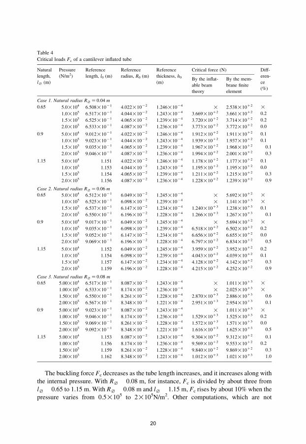
Table 4
Critical loads Fc of a cantilever inflated tube
Natural
length,
l: (m)
Pressure
(N/m2)
Reference
length, l0 (m)
Reference
radius, R0 (m)
Reference
thickness, h0
(m)
Critical force (N) Diff-
eren-
ce
(%)
By the inflat-
able beam
theory
By the mem-
brane finite
element
Case 1. Natural radius R: Z0:04 m
0.65 5.0!104 6.508!10K1 4.022!10K2 1.246!10K4 ! 2.538!10C2 !
1.0!105 6.517!10K1 4.044!10K2 1.243!10K4 3.669!10C2 3.661!10C2 0.2
1.5!105 6.525!10K1 4.065!10K2 1.239!10K4 3.720!10C2 3.714!10C2 0.2
2.0!105 6.533!10K1 4.087!10K2 1.236!10K4 3.773!10C2 3.772!10C2 0.0
0.9 5.0!104 9.012!10K1 4.022!10K2 1.246!10K4 1.912!10C2 1.911!10C2 0.1
1.0!105 9.023!10K1 4.044!10K2 1.243!10K4 1.939!10C2 1.937!10C2 0.1
1.5!105 9.035!10K1 4.065!10K2 1.239!10K4 1.967!10C2 1.968!10C2 0.1
2.0!105 9.046!10K1 4.087!10K2 1.236!10K4 1.994!10C2 2.001!10C2 0.3
1.15 5.0!104 1.151 4.022!10K2 1.246!10K4 1.178!10C2 1.177!10C2 0.1
1.0!105 1.153 4.044!10K2 1.243!10K4 1.195!10C2 1.195!10C2 0.0
1.5!105 1.154 4.065!10K2 1.239!10K4 1.211!10C2 1.215!10C2 0.3
2.0!105 1.156 4.087!10K2 1.236!10K4 1.228!10C2 1.239!10C2 0.9
Case 2. Natural radius R: Z0:06 m
0.65 5.0!104 6.512!10K1 6.049!10K2 1.245!10K4 ! 5.692!10C2 !
1.0!105 6.525!10K1 6.098!10K2 1.239!10K4 ! 1.141!10C3 !
1.5!105 6.537!10K1 6.147!10K2 1.234!10K4 1.240!10C3 1.238!10C3 0.1
2.0!105 6.550!10K1 6.196!10K2 1.228!10K4 1.266!10C3 1.267!10C3 0.1
0.9 5.0!104 9.017!10K1 6.049!10K2 1.245!10K4 ! 5.694!10C2 !
1.0!105 9.035!10K1 6.098!10K2 1.239!10K4 6.518!10C2 6.502!10C2 0.2
1.5!105 9.052!10K1 6.147!10K2 1.234!10K4 6.656!10C2 6.655!10C2 0.0
2.0!105 9.069!10K1 6.196!10K2 1.228!10K4 6.797!10C2 6.834!10C2 0.5
1.15 5.0!104 1.152 6.049!10K2 1.245!10K4 3.959!10C2 3.952!10C2 0.2
1.0!105 1.154 6.098!10K2 1.239!10K4 4.043!10C2 4.039!10C2 0.1
1.5!105 1.157 6.147!10K2 1.234!10K4 4.128!10C2 4.142!10C2 0.3
2.0!105 1.159 6.196!10K2 1.228!10K4 4.215!10C2 4.252!10C2 0.9
Case 3. Natural radius R: Z0:08 m
0.65 5.00!104 6.517!10K1 8.087!10K2 1.243!10K4 ! 1.011!10C3 !
1.00!105 6.533!10K1 8.174!10K2 1.236!10K4 ! 2.025!10C3 !
1.50!105 6.550!10K1 8.261!10K2 1.228!10K4 2.870!10C3 2.886!10C3 0.6
2.00!105 6.567!10K1 8.348!10K2 1.221!10K4 2.951!10C3 2.954!10C3 0.1
0.9 5.00!104 9.023!10K1 8.087!10K2 1.243!10K4 ! 1.011!10C3 !
1.00!105 9.046!10K1 8.174!10K2 1.236!10K4 1.529!10C3 1.525!10C3 0.2
1.50!105 9.069!10K1 8.261!10K2 1.228!10K4 1.572!10C3 1.571!10C3 0.0
2.00!105 9.092!10K1 8.348!10K2 1.221!10K4 1.616!10C3 1.625!10C3 0.5
1.15 5.00!104 1.153 8.087!10K2 1.243!10K4 9.304!10C2 9.312!10C2 0.1
1.00!105 1.156 8.174!10K2 1.236!10K4 9.569!10C2 9.553!10C2 0.2
1.50!105 1.159 8.261!10K2 1.228!10K4 9.840!10C2 9.869!10C2 0.3
2.00!105 1.162 8.348!10K2 1.221!10K4 1.012!10C3 1.021!10C3 1.0
The buckling force Fc decreases as the tube length increases, and it increases along with
the internal pressure. With R: 0:08 m, for instance, Fc is divided by about three from
l: 0:65 to 1.15 m. With R: 0:08 m and l: 1:15 m, Fc rises by about 10% when the
pressure varies from 0.5!105 to 2!105N/m2. Other computations, which are not
20

Fig. 4. Critical loads of a cantilever. (†) inflatable beam theory, ( ) membrane finite element, ( $ $ ) crushing
force.
presented here, show that the influence of the pressure on the buckling force is stronger if a
material with lower Young modulus is chosen. Nevertheless, the strains can then be so
large that a fully non-linear computation is required.
If the pressure were not taken into account, the discrepancy between the beam theory
and the membrane finite element computation should reach 4.1%. Furthermore, if the
correction coefficient k is given very large values (one then reduces to then Euler
Bernoulli model), then the discrepancy reaches 13.4%.
6. Conclusions
The non-linear equations have been derived for the in-plane stretching and bending
of an inflated Timoshenko beam undergoing finite rotations. The corresponding
linearized equations have been obtained and then analytically solved for the bending
21

and the buckling cases. New theoretical and numerical results on the buckling of
inflatable beams are displayed. The following facts have been emphasized.
(i) It is crucial to distinguish between the so-called natural configuration where the
internal pressure is zero and the pre-stressed reference configuration around
which the linearization is performed. The dimensions defining the reference
configuration of the beam depend on the prescribed internal pressure.
(ii) The analytical solutions have clearly shown the beneficial effects of the internal
pressure on the bearing capacity of the beam: the inflation amounts to increasing
the material properties.
(iii) The analytical solution for the bent beam only holds if the pressure is greater
the so-called wrinkling pressure. Similarly, the solution for the buckled beam is
valid only if the compressive force is less than the so-called crushing force.
The numerical computations have been performed on nine beam geometries (three
values of natural radius by three values of natural length) and four values of the internal
pressure. The maximum deflections or the buckling forces have been found to be in good
agreement with the membrane finite element values obtained within the three-dimensional
framework.
Further investigations are in progress in order to obtain analytical solutions in dynamics
and derive finite elements for solving complex geometries and loadings of inflated beams.
References
[1] Comer RL, Levy S. Deflections of an inflated circular cylindrical cantilever beam. AIAA J 1963;1(7):1652 5.
[2] Fichter WB. A theory for inflated thin wall cylindrical beams. NASA TN D 3466; 1966.
[3] Main A, Peterson SW, Strauss AM. Load deflection behaviour of space based inflatable fabric beams.
J Aerospace Eng 1994;2(7):225 38.
[4] Wielgosz C, Thomas JC. Deflections of inflatable fabric panels at high pressure. Thin Walled Struct 2002;40:
523 36.
[5] Thomas JC, Wielgosz C. Deflections of highly inflated fabric tubes. Thin Walled Struct 2004;42:1049 66.
[6] Wielgosz C, Thomas JC. An inflatable fabric beam finite element. Commun Numer Meth Eng 2003;19:
307 12.
[7] Cowper GR. The shear coefficient in Timoshenko’s beam theory. J Appl Mech 1967;33:335 40.
22