1

Benchmark Status in Fixed-Income Asset Markets

Peter G. Dunne*

Queen's University, Belfast, Northern Ireland

Michael J. Moore

Queen's University, Belfast, Northern Ireland

Richard Portes

London Business School and CEPR

This version: 2 February 2007

Abstract

What is a benchmark bond? We provide a formal theoretical treatment of this concept that relates endogenously determined benchmark status to price discovery and we derive its implications. We describe an econometric technique for identifying the benchmark that is congruent with our theoretical framework. We apply this to the US corporate bond market and to the natural experiment that occurred when benchmark status was contested in the European sovereign bond markets. We show that France provides the benchmark at most maturities in the Euro-denominated sovereign bond market and that IBM provides the benchmark in the US corporate bond market.

Keywords: Price discovery, benchmark, bond market, cointegration. JEL Classification: F36, G12, H63

* The address for correspondence is: Michael J. Moore, School of Management and Economics, Queen’s University, Belfast, Northern Ireland BT7 1NN, United Kingdom, Tel +44 28 90273208, Fax +44 28 90335156, email m.moore@qub.ac.uk. We are grateful for comments from Lasse Pedersen, Jim Davidson, David Goldreich, Stephen Hall, Harald Hau, Rich Lyons, Kjell Nyborg and Carol Osler. This paper is part of a research network on ‘The Analysis of International Capital Markets: Understanding Europe’s Role in the Global Economy’, funded by the European Commission under the Research Training Network Programme (Contract No. HPRNŒCTŒ1999Œ00067). We thank Euro-MTS Ltd for providing the data and Kx Systems, Palo Alto, and their European partner, First Derivatives, for providing their database software Kdb.

2

1. Introduction

Euro-denominated sovereign bonds have highly correlated yields and are

generally regarded as very close substitutes for each other. Corporate bonds mainly

differ from each other in regard to their credit-risk but even credit risk is known to

have common components (see Driessen, 2005). Where there is such extreme

similarity across an asset class, market participants’ risk exposure and hedging

requirements can be met from a sub-set of the class. In this case liquidity usually

concentrates on a small number of individual cases and we observe that these are

often selected as reference points for the market as a whole. Sometimes this is

explicit, as when yields displayed on electronic platforms are expressed as spreads

over a reference security. With liquidity so concentrated most of the asset class

becomes very illiquid and it becomes difficult to construct reliable indices that would

normally be used for pricing. This creates and reinforces the need for an alternative

reference point and opens the way for a single asset to take the role as benchmark.

It seems reasonable to expect that when a reference security emerges it would

attract more liquidity and become the location of price-discovery for market-wide

phenomena. Once a security can be identified as being a source of price-discovery in

this way, network externalities can play a role in reinforcing its position. Thus,

liquidity is as much an outcome as a cause of benchmark status. Yuan (2005)

proposed the idea that benchmark status relates to price-discovery for the market as a

whole. Yuan’s definition highlights the benchmark security’s sensitivity to

systematic risk, as opposed to asset-specific risk, as central to its identification. We

modify Yuan’s model to derive a condition that identifies a single bond as the

benchmark.

3

In common with Yuan, our model and empirical approach associates

benchmark status with the price-discovery process rather than with either the level of

the yield or the liquidity of the issue (see Hasbrouck, 1995, for a treatment in the

context of equity markets). We contend that a single bond is most likely to emerge as

a benchmark when there is an asset with a significant sensitivity to systematic

variability and insignificant idiosyncratic variability. As a focus for market-wide

price discovery the benchmark will improve as a reference point because it will lead

what happens elsewhere in the market. The likelihood that a benchmark will arise

also depends on how deficient the alternative (i.e., an index) is likely to be and on

how expensive it is to trade the index. The prevalence of OTC trading will also tend

to reduce the quality of an index because so many prices are hidden. And where a

suitable, single-asset, benchmark candidate exists and becomes established, the

constituents of a potential index may be degraded by insufficient liquidity to the point

of reinforcing the benchmark.

The model is consistent with the view that the benchmark security provides an

information externality to the market as a whole because it represents common

movements of the entire market without noise. In essence a benchmark security arises

out of the market’s need for a focus for market-wide price-discovery and concentrates

the aggregation of information reducing the costs of information acquisition in all

markets where a security is traded against the benchmark.

Alternative views exist regarding the qualities associated with benchmark

status. For example, in the case of euro-denominated sovereign bonds the benchmark

has often been assumed to be the lowest yielding bond at each maturity and this has

invariably been the German one (e.g., Favero et al., 2000, pages 25-26). The

benchmark has also been interpreted to mean the most liquid security (see Blanco

4

2002) which is therefore most capable of providing a regular reference point for the

market. But in the Euro-denominated sovereign bond market the Italian, not the

German, are easily the largest and most liquid issues and yet they are seldom regarded

as having benchmark status.

Krishnamurthy and Vissing-Jorgensen (2006) also attribute a convenience

yield to US Treasuries which they associate with liquidity attributes and to the

perceived low-risk status of Treasuries. Our analysis suggests that this convenience

yield also derives from the fact that idiosyncratic innovations in Treasury yields are

either infrequent or fully expected because of transparent monetary policy.

Essentially, Treasuries have most of the qualities we associate with benchmark status.

Thus, while liquidity and other attributes may play a role, our theory calls for a more

formal approach to identification of benchmark status. Benchmark status cannot just

be asserted on the basis of underlying liquidity, credit worthiness or the level of the

yield.

Apart from the positive information externality there are other reasons why

identifying a benchmark could be of benefit. In the context of the MiFID proposals of

the European Commission’s ‘Financial Services Action Plan’, sell-side agents are

under pressure to demonstrate that they have delivered ‘best-execution’ on

transactions in infrequently traded assets (Commission Directive 2006/73/EC). The

existence of a reliable benchmark and the ability to derive a reference price that is

relevant to each security is potentially of great benefit in this case. Additionally, in

the increasingly important area of ‘fair-value’ accounting for financial instruments,

the International Accounting Standards Board (IASB, 2005) sets out a conceptual

framework for determining fair-values for initial recognition in financial statements.

‘Level-2’ in the ‘measurement hierarchy’ is described by IASB in the following

5

terms: “If observable market prices for identical assets or liabilities are not available

on the measurement date, fair-value shall be estimated using observable market prices

for similar assets or liabilities adjusted as appropriate for differences, whenever that

information is available.” Our methodology provides a basis for implementing such

an approach.

An additional motivation for our study arises from the implementation of

monetary policy in the euro area. One legacy of the introduction of the euro has been

the growing recognition of the need to broaden the scope of open market operations.

The European Central Bank currently concentrates on the swaps and repo market to

implement its monetary policy. In its ‘General documentation on Eurosystem

monetary policy instruments and procedures (2002)’, however, the ECB refers to the

possible need for structural operations that may be required to influence the market’s

liquidity position over long horizons. Our analysis has a bearing on the choice of

policy instrument.

Finally, if benchmark status increases the liquidity of an issue and provides

convenience to market participants then it will attract a convenience premium. This is

attractive for the issuer seeking to reduce the cost of borrowing. Our analysis

highlights those aspects of policy that can aid in the acquisition of benchmark status.

The minimization of idiosyncratic innovations, rather than the augmentation of the

systematic component of yields, is what matters most. In the sovereign bond case,

this would require an issuer to produce as few country-specific policy innovations as

possible. Building a reputation for stability (never surprising the market with

idiosyncratic movements) allows market participants to look ahead with some

confidence in the benchmark properties of an issue. There is also some benefit to be

6

had from improving and maintaining the liquidity of an issue since this will improve

the speed with which the security can reflect market-wide developments.

The existing empirical approaches to identifying the price discovery process

are limited. Scalia and Vacca (1999), for example, use Granger-causality tests to

determine whether price discovery occurs in the cash or futures market in Italian

bonds. In the context of identifying benchmark status, however, we believe that

Granger-Causality testing exhibits significant weaknesses, particularly for high-

frequency transaction data with variable liquidity. First, it can be inconclusive

because series can Granger-cause each other. Second, Granger-causality is about

dynamics: it has nothing to say about long-run relationships between series1.

We also acknowledge that if a reliable index is available, then there are

various ways of identifying which individual security is the best representation of that

index. For example, it would be straightforward to select the security that had highest

measured correlation with the index. This strategy is redundant however when a

reliable index is unavailable. The approach we invoke is suitable when liquidity

concentrates on a small subset of the asset-class and renders any index constructed

using the entire class as unreliable and redundant.

Our empirical method exploits the fact that yields are empirically

indistinguishable from non-stationary processes. If there were a unique benchmark at

every maturity, then we would expect that the yields of other bonds would be

cointegrated with that benchmark. Indeed, there should be multiple cointegrating

vectors centering on the benchmark bond. Our empirical approach relies on a result,

based on Davidson (1998), that the structural nature of the cointegrating relationship

between a benchmark bond and other bonds can be identified even in the context of

quite a general theoretical framework.

7

We apply this methodology to two interesting cases where benchmark status is

of topical interest due to the concentration of liquidity and the patent lack of reliable

and unrepresentative indices. The first application concerns the identification of the

benchmark in the euro-denominated sovereign bond market where benchmark status

was uncertain following the introduction of the euro. The second application

concerns benchmark status in the US corporate bond market where the TRACE

system has increased post-trade transparency making it easier for a benchmark to be

identified by market participants. In the case of corporate bonds, we show that the

benchmark can be identified despite the presence of differential credit risk. However,

to achieve this, our methodology must be modified to include information about

credit-default. We use credit default swap data to assist in this application.

In the next section, we provide an explicit theoretical framework within which

a benchmark security is defined. Section 3 presents the novel empirical methodology.

The results from applying this to the euro-area bond market are presented in section 4.

An application to the US corporate bond market is contained in Section 5. Section 6

contains concluding remarks and directions for future research.

2. Benchmark securities: a formal framework

Yuan (2005) formalises the concept of a benchmark security and we begin by

adapting this definition to the non-stationary case.

Consider a fixed-income security as having a yield with the following factor

structure2:

% 1.....,i i ir i nβ γ ε= + = (1)

8

where ir is the nominal yield on the ith security, %γ is a systematic factor and iβ is

security i’s sensitivity to the systematic factor. iε is the idiosyncratic shock.

Conventionally, factor pricing models place very little emphasis on issues of

stationarity3. However, bond yields are typically found to be indistinguishable from

non-stationary processes and so we modify Yuan’s model by identifying the source of

the non-stationarity as the systematic factor %γ which we assume is a general I(1)

process4 with innovations µ% . Consequently, all of the yields are themselves non-

stationary.

The security specific shocks 1.....,i i nε ∀ = are assumed to be stationary

ARMA processes:

( )i i iB Lε η= (2)

The parameters of the ARMA process ( )iB L are also security-specific, and the iη are

independently distributed with mean zero and constant variance 2iσ . We also assume

that ( ) 0iE iη µ = ∀% % .

At this point, we require the following Lemma:

Lemma 1. All pairs of security yields { }, 1....,ir i n= are cointegrated. Proof: For

any and i jr r equation (1) implies that

j ji i

i j i j

rr εεβ β β β

⎛ ⎞− = −⎜ ⎟⎜ ⎟

⎝ ⎠

The right hand side is stationary by construction. The cointegrating vector is

1 1,i jβ β

⎛ ⎞−⎜ ⎟⎜ ⎟

⎝ ⎠■

The variance of the cointegrating residual is:

9

( ){ } ( ){ }2 22 2

2 2Var i i j jji

i j i j

B L B Lrr σ σ

β β β β⎛ ⎞

− = +⎜ ⎟⎜ ⎟⎝ ⎠

(3)

We now introduce a formal definition of a benchmark security:

Definition 1: A benchmark security has no dependence on idiosyncratic risk

This definition is obviously idealised and immediately leads to the following

b br β γ= % (4)

where the subscript b refers to the benchmark.

This is the idea that, where a common non-stationary factor exists and there exists a

security which has sensitivity (not necessarily unitary) to this factor and little or no

idiosyncratic innovations, then the conditions for the emergence of a benchmark are

in place. The key element for the emergence of the benchmark is the absence (or

insignificance) of idiosyncratic risk.

The next lemma follows directly from Lemma 1: .

Lemma 2. All security yields { }, 1....,ir i n= are pairwise cointegrated with the

benchmark yield br .

Proof:

From equations (1) and (4),

i b i

i b i

r r εβ β β

− =

The right hand side is stationary by assumption. The cointegrating vector is

1 1,i bβ β

⎛ ⎞−⎜ ⎟

⎝ ⎠■

10

The variance of the cointegrating residual is:

( ){ }2 2

2Var i ii

i i

B L σεβ β

⎧ ⎫⎪ ⎪ =⎨ ⎬⎪ ⎪⎩ ⎭

(5)

We can now state the main result:

Theorem 1:

The variance of the residual error in the cointegrating vector between security i’s

yield and any other security j=1,…,n, ≠ b, is always greater than the variance of the

residual error in the cointegrating vector between security i’s yield and the

benchmark yield.

Proof: Compare equations (3) and (5). ■

Although the conditions set out above are quite restrictive, they are in our

view essential for the emergence of a benchmark security. In particular, if a security

has benchmark potential it must be the case that it is not excessively compromised by

non-systematic noise. If an asset with these properties cannot be identified then it is

unlikely that a benchmark will emerge. The benchmark must also become central to

price-discovery or at least be quick and accurate in reflecting market-wide

phenomena. These requirements suggest why benchmark status is occasionally

uncertain and contested. This is due to the arrival of unexpected idiosyncratic shocks

that render the existing benchmark unreliable as a pricing reference and undermine

confidence in its expected future relevance. Although it is tempting to associate the

benchmark thus defined with a low yielding bond this is not necessarily the case since

bβ could be relatively high. In the euro-denominated sovereign bond market, for

example, an absence of idiosyncratic innovations would suggest that the benchmark is

likely to be associated with a very central player in the monetary union or one that is

very committed to the union.

11

The above analysis has made no reference to credit default risk. This is hardly

a significant omission in the cases of the sovereign markets of the euro-zone or the

US. However, credit default is a serious issue for the corporate bond market. In

particular, it would be heroic to assume that the non-stationary component of asset-

specific default and credit risk could be entirely represented by sensitivity to a single

non-stationary systematic factor. While the work of Driessen (2005) shows that there

is evidence of systemic credit risk across corporate bonds, there is no suggestion in

the literature that this represents all systematic risk or that all idiosyncratic non-

stationary credit risk could be derived by way of sensitivity to this common

component alone. However, idiosyncratic (perhaps non-stationary) credit risk can be

observed from corporate bond ‘credit default swap’ (CDS) markets and we propose to

use this information to control for asset-specific factors in our empirical application to

US corporate bonds.

The benchmark derived, having controlled for these observable CDS spreads,

can be interpreted as best representing market-wide price-discovery with regard to the

remaining non-stationary common factor. This could be associated with non-default

components of the corporate bond spread as described by Krishnamurthy and Vissing-

Jorgensen (2006) and identified by a number of other recent contributions to the

corporate bond-pricing literature including Collin-Dufresne, Goldstein, and Martin

(2001), Huang and Huang (2001), and Longstaff, Mithal, and Neis (2006). In the case

of Krishnamurthy and Vissing-Jorgensen, the variation in the corporate spread is the

convenience yield on Treasuries but, since we consider yields rather than yield

spreads, in our case it can be considered to encompass both the convenience yield of

treasuries and other non-default components.

12

3. Econometric Methodology

The factor definition of a benchmark in Section 2, along with Lemmas 1 and 2 and

Theorem 1, suggests that the benchmark should be identified from an analysis of the

cointegration properties of the yield series. If a particular security is the benchmark at

a given maturity, then there should be two cointegrating vectors in a three-variable

system of security yields. The usefulness of this however is compromised by the

presence of an identification problem. Even if we are satisfied that such cointegration

vectors exist, we cannot draw any immediate conclusion about the structure of the

relationships between yields, such as the identity of the benchmark, because any

linear combination of multiple cointegrating vectors is itself a cointegrating vector.

A parallel development in non-stationary econometrics due to Davidson

(1998) and developed by Barassi, Caporale and Hall (2000a,b) provides the empirical

analogue of the theory laid out in Section 2 above. This approach tests for

irreducibility of cointegrating relations and ranks them according to the criterion of

minimum variance. The interesting feature of this method is that it allows us to learn

about the structural relationship that links cointegrated series from the data alone,

without imposing any arbitrary identifying conditions. In this case, the ‘structural’

relationship is simply the identity of the benchmark in a set of bond yields.

There is a risk of confusion in the use of the word ‘structure’, which has many

different uses in the literature. In Davidson’s approach, it refers to parameters or

relations that have a direct economic interpretation and may therefore satisfy

restrictions based on economic theory. It need not mean a relationship that is regime-

invariant. The possibility that “incredible assumptions” (Sims, 1980) need not always

13

be the price of obtaining structural estimates turns out to be a distinctive feature of

models with stochastic trends.

According to Davidson (1998) an irreducible cointegrating vector can be

defined as follows:

Definition 2 (Davidson): A set of I(1) variables is called irreducibly cointegrated

(IC) if they are cointegrated, but dropping any of the variables leaves a set that is not

cointegrated.

Following from this definition, IC vectors can be divided into two classes: structural

and solved. A structural IC vector is one that has a direct economic interpretation.

More specifically:

Theorem 2 (Davidson). If an IC relation contains a variable which appears in no

other IC relation, it is structural.

The less interesting solved cointegrating vectors are defined as follows:

Definition 3 (Davidson). A solved vector is a linear combination of structural vectors

from which one or more common variables are eliminated by choice of offsetting

weights such that the included variables are not a superset of any of the component

relations.

Thus, a solved vector is an IC vector which is a linear combination of structural

IC vectors. Once an IC relation is found, we wish to distinguish between structural

and solved forms. The key point is that we can identify the structure from the data

directly.

14

The BCH extension of Davidson's framework can be illustrated concretely as

follows. In a system made up of three I(1) variables, say the French, German and

Italian bond yields, consider the case where the German-French yield pair and the

German-Italian yield pair are both cointegrated. It follows necessarily that the French-

Italian pair is also cointegrated. The cointegrating rank of these three variables is 2,

and one of these three IC relations necessarily is solved from the other two. The

problem is that we cannot know which. The BCH methodology gives an (almost)

unambiguous answer. In order to detect which of the cointegrating relations is the

solved one and which of the vectors are irreducible and structural, we calculate the

descriptive statistics of each cointegrating relation and rank these vectors on the basis

of the magnitude of the variance of their residual errors. The structural vectors emerge

as those corresponding to the lowest variance. The reason for this is suggested by

standard statistical theory and can be illustrated as follows. Let G, F and I be our

cointegrated series. Suppose G provides the benchmark so that the first two of the

following equations can be considered ‘structural relations’ while the third is ‘solved’.

1 1

2 2

2 3

F G eI G eI F e

βββ

= += += +

(6)

Now 1e and 2e , being the structural error terms are assumed5 to be distributed

independently ( )2iN 0,σ , 1, 2i = . The third equation is just solved from the first two.

This implies that 3e is a function of 1e and 2e , and therefore we expect it to be

distributed 2

2 221 22

1

N 0, β σ σβ

⎛ ⎞+⎜ ⎟

⎝ ⎠. Note that this is always greater than 2

2σ and

if { }2 2 21 2 3 1 2 then ,Maxβ β σ σ σ≤ > . The solved variance can only be smaller than the

15

structural if 2 22 1σ σ< and if

222

1

ββ

is small enough such that ( )2

2 2 221 1 22

1

β σ σ σβ

< − . For this

to be empirically significant, we require that either 1 2or β β diverge considerably

from unity. Therefore cointegrating relations whose residuals display lower variance

should almost always be the structural ones, the remaining others being just solved

cointegrating relations. This result simply mirrors the statement of Theorem 1 in

Section 2.

4. Application: Contested benchmark status in the Euro-denominated sovereign

bond market

The introduction of the euro on 1 January 1999 eliminated exchange risk

between the currencies of participating member states and thereby created the

conditions for a substantially more integrated public debt market in the euro area.

The euro-area member states agreed that from the outset, all new issuance should be

in euro and outstanding stocks of debt should be re-denominated into euro. As a

result, the euro-area debt market is comparable to the US treasuries market both in

terms of size and issuance volume (see Galati and Tsatsaronis 2001; Blanco 2001).

Despite the homogenizing effects of the euro in terms of exchange rate risk,

public debt management in the euro area remained decentralised under the

responsibility of 12 separate national agencies. This decentralised management of the

euro-area public debt market is one reason for cross-country yield spreads. McCauley

(1999) draws some comparisons between the US municipal bond market and the euro

government bond markets. But the evidence of differentiation across countries has

not been thoroughly explored (see Codogno et al. 2003; Portes 2003). It is clear from

16

Blanco (2001), however, that in the initial years of the euro, yields were normally

lowest for German bonds; that there was an inner periphery of countries centred on

France for which yields were consistently higher; and that the outer periphery centred

on Italy displayed the highest yields.

The significant levelling of the playing field brought about by the introduction

of the euro was expected to impact on concentration in trading activity across the

more liquid and lower default-risk bonds or in the bonds that were deliverable on

futures contracts. Since much of the trading in these bonds remains OTC it is difficult

to assess how concentrated liquidity was. The recent work by Dunne et al. (2006)

indicates that liquidity has been surprisingly well spread within and across country-

specific bonds on the MTS inter-dealer trading platform. This is largely due to the

use of Primary Dealer Systems (PDS) by the issuers. A significant element of the

PDS is the imposition of obligations on the primary dealers to provide liquidity on the

MTS trading system.

Nevertheless, this is a relatively recent development and, as described by

Galati and Tsatsaronis (2001), there was a period of competition between issuers over

benchmark status at each maturity at the inception of the monetary union. While the

existence of a very liquid futures market in German bunds favoured German bonds as

benchmark, the fact that these bonds were not issued in great size at short and medium

maturities introduced a significant element of uncertainty regarding benchmark status

at these maturities. We now examine which country empirically appears to provide

the benchmark in this period of contested benchmark status.

17

4.1 Data

We have a unique data set from Euro-MTS for 1 April 2003 to 31 March

2005. We use daily data for this period. Since the creation of the euro in 1999, Euro-

MTS has emerged as the principal electronic trading platform for bonds denominated

in euros. Already by the end of 2000, it was handling over 40% of total transactions

volume (Galati and Tsatsaronis, 2001). Government bonds traded on Euro-MTS must

have an issue size of at least €5 billion. For a discussion of MTS, see Scalia and

Vacca (1999) and DeJong et al. (2004). It is possible to obtain a clearer and more

recent estimate of the MTS share of the market by reference to Dunne et al. (2006).

In the case of the Italian market, all trading is legally required to be conducted on the

MTS trading platform so our Italian coverage is 100% of the trading in Italian bonds.

The Italian market provides a useful guide as to the likely overall trading

volume in non-Italian bonds. The study by Dunne et al. (2006) shows that, in

December 2003, the MTS traded volume as a percentage of the amount outstanding

for the three most recently issued 10 year Italian bonds, ranged between 12.19% and

34.37%. The highest percentages for the equivalent French and German 10 year

bonds were 2.74% and 3.76% respectively. Thus, even if the actual turnover in

French and German bonds was as low as 12.19%, this implies MTS shares of overall

trading equal to 23% in the case of France and 30% in the case of Germany. While

this implies that the French and German bonds are not well represented on MTS it is

the case that this platform is virtually the only, and certainly the most visible, source

of pre- and post-trade information in this market and we contend that it represents the

only viable location for a benchmark.

18

We selected data from France, Germany and Italy. Together the three

countries account for over 70% of the euro-zone market (Blanco, 2001). We found

that the coverage of the data for the other euro-zone countries was too sparse to get a

consistently clear picture of even daily activity. In the analysis below we examine

bonds from within four maturity buckets6. Within each maturity, we select the bond

that is most recently issued for each country. This rule is applied on a 3-month basis,

so that the bond used in the analysis can change a number of times over the two years

of our study. At the long and very long maturities, for each country, the same bond

was both available and liquid throughout the two-year sample. For the short and

medium maturities, there were frequent changes of bonds, both because bonds

changed maturity bracket or went off-the-run. In our empirical work we included

shift dummies to account for bond changes of this kind. The daily observation for

each country and maturity was chosen as the final mid-quote at the 16.30 close. We

used the mid-quote to avoid spurious bid-ask bounce. It is important to emphasise

that the quotes are not indicative but executable.

4.2 Results

For each maturity, each bond yield is subjected to a Dickey-Fuller test for

stationarity. The results are reported in Table 1. The outcome of the tests is simple

to summarise. In every case, non-stationarity7 of the yield cannot be rejected.

In this light, our empirical strategy is as follows. First, we use the Johansen8

procedure to identify the number of cointegrating vectors at each maturity in our

three-variable system. Then, we use Phillips-Hansen fully modified estimation to

estimate the irreducible cointegrating vectors as recommended by Davidson. Finally

19

we rank the irreducible cointegrating vectors using the variance-ranking criterion of

BCH. From this we identify the structural vectors and therefore the benchmark. The

latter must be the common yield in the two structural irreducible cointegrating

vectors. The results are shown for each maturity in Tables 2 to 5.

(i) Johansen Procedure:

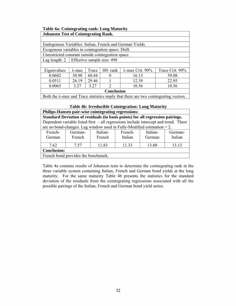
In Tables 2a, 3a, 4a and 5a, it is clear that there are two cointegrating vectors

among the three yields at the short, medium, long and very long maturities. This can

be read from comparing the ‘λ-max’ and ‘trace’ test statistics to their critical values

which we reproduce for convenience. Consequently, we conclude that all yields are

pairwise cointegrated.

(ii) Irreducible cointegration vectors and BCH minimum variance ranking:

Regressions for each pair of yields were carried out using Phillips Hansen

Fully Modified Estimation. To ensure that the choice of dependent variable does not

matter we obtained estimates for each possible choice of dependent variable in each

pairing. This amounts to six regressions for each maturity, 24 in all. Full details of

the regressions are available on request. For each maturity, Tables 2b, 3b, 4b and 5b

report the residual standard error of each regression. The results are summarised here

by each maturity.

Short: The standard deviation of the residuals of the six cointegrating vectors varies

from 9.10 to 30.97 basis points. The highest two arise from the regression of the

Italian on the German yield and vice versa. From this we conclude that that the

20

French-German and Italian-French relationships are structural and that the French

yield provides the benchmark at the short end.

Medium: The standard deviation of the residuals of the six cointegrating vectors

varies from 8.78 to 12.02 basis points. As with the short maturity, the highest two

arise from the regression of the Italian on the German yield and vice versa. From this

we conclude that that the French-German and Italian-French relationships are

structural and that the French yield provides the benchmark at the medium maturity.

Long: The standard deviation of the residuals of the six cointegrating vectors varies

from 7.57 to 13.80 basis points. Once again, the highest two arise from the regression

of the Italian on the German yield and vice versa. From this we conclude that that the

French-German and Italian-French relationships are structural and that the French

yield provides the benchmark at the long end.

Very Long: It is clear that French-German pair provides us with the lowest residual

standard deviation irrespective of the choice of dependent variable. However, the

range of the residual variances for the Italian-French and the German-Italian pairings

overlap. This therefore is a case where the conditions for selection of the benchmark

are not unambiguously met. All we can definitely conclude is that Italy does not

provide the benchmark. While the assumption that France provides the benchmark is

not contradicted, we cannot reach a definite ranking of pairs. From this we conclude

that benchmark status is contested at the very long maturity between France and

Germany.

21

5. Application: The search for a benchmark in the US Corporate bond market

In this section we consider the identification of a single-asset benchmark in the

US corporate bond context. The purpose of this example is to demonstrate that the

technique can be expanded to a wider range of assets so long as it is possible to

account for idiosyncratic, non-stationary components. In the case of corporates, the

asset-specific effects can be rolled-into the analysis by using credit default swap

spreads.

The earlier methodology need only be adjusted by the inclusion of exogenous

variables representing idiosyncratic non-stationary components (CDS spreads).

Having controlled for these variables we expect corporate yields to be pair-wise

cointegrated. We also expect the pairings with the benchmark asset to possess the

lowest residual variance from the cointegrating regressions. In this case we do not

consider Johansen ML regressions since this would not really provide us with useful

information (i.e., we do not necessarily have priors to test regarding the cointegrating

rank between all the corporate yields and their CDS spreads). What we propose

instead is to consider whether corporate yields are non-stationary and whether they

are pair-wise cointegrated conditional on CDS spreads. Once this is established we

can proceed to assess which of the assets appears to provide the benchmark based on

the minimum variance technique.

5.1 Corporate bond and CDS Data

There are many agencies that identify a sub-class of corporate bonds as, in

some sense, providing a benchmark (e.g., JPMorgan, US Liquid Corporate Index and

CreditTrade’s Benchmark American Corporates). These generally make some

22

reference to the liquidity of the constituents and/or their investment grade. We take

CreditTrade’s list of US benchmarks as a starting point in the search for a ‘price-

discovery-based’ benchmark. We focus on a narrow industry grouping

(manufacturing/technology) and on a maturity category (roughly 10 years to

maturity). In this industry category there were 14 corporate entities classified as

benchmarks. Of these only 4 were in the 10 year to maturity category and we

dropped one of these because it was not frequently traded (as revealed by the TRACE

system). This provides us with a corporate analogue to the sovereign case analyzed

above (details regarding these corporates is given in the appendix).

For the 3 corporate entities chosen as potential benchmarks we obtained daily

data from the Thomson Financial DATASTREAM research database for a period

running from 21 March 2005 to 17 Oct 2006. The corporate yield data is sourced

from FT Interactive Data and this provides an end-of-day ‘evaluated price’ in each

case. The CDS data is sourced from CMA records and provides an implied end-of-

day yield spread based on the average mid-price between bid-offer quotes for CDS

premia collected from a number of CDS dealers9.

5.2 Results

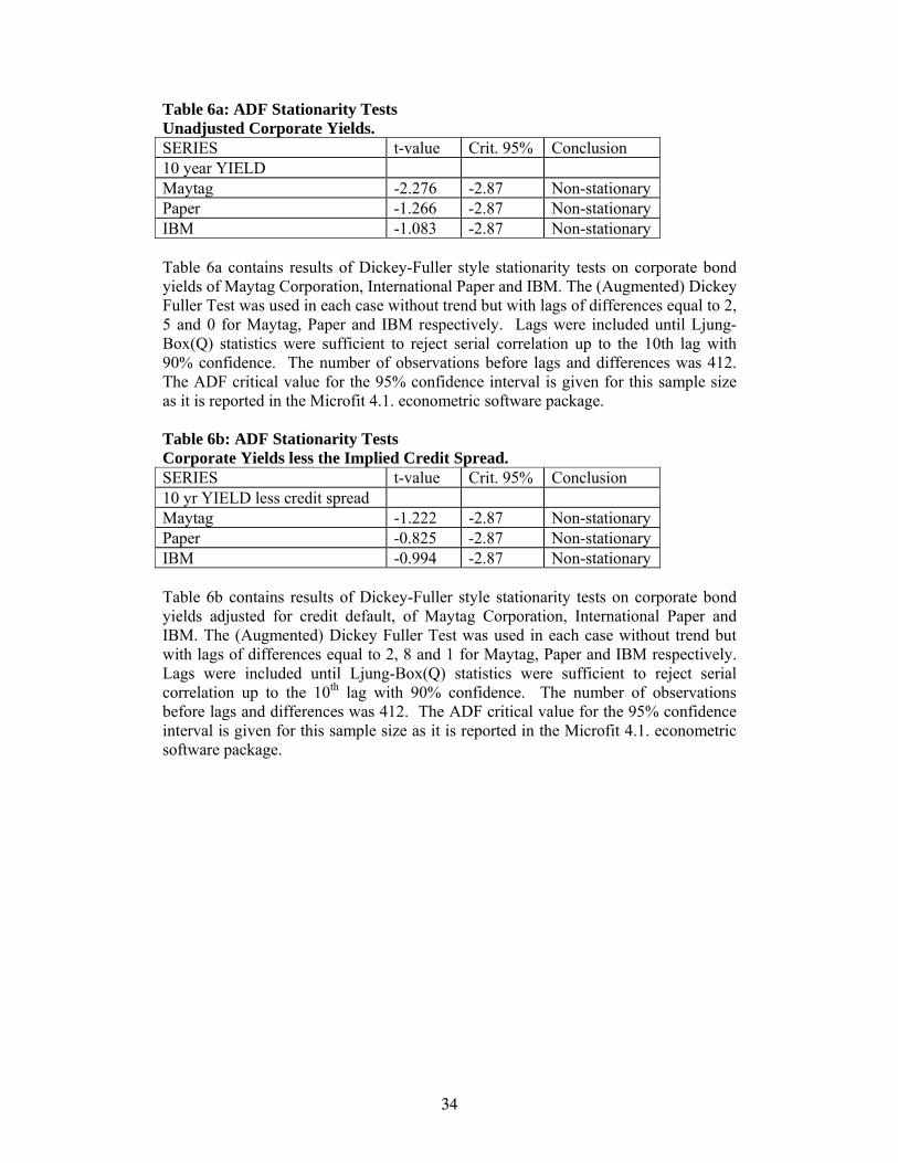
ADF stationarity test results for the corporate yields are shown in Table 6a.

This clearly indicates that non-stationarity cannot be rejected for all of the yields10.

What is more interesting is the evidence of non-stationarity of the yields when

adjusted by subtraction of the implied credit risk premium as shown in Table 6b.

Credit risk is not therefore the only source of non-stationarity in corporate yields and

therefore it is of interest to consider whether what is left-over contains a common

23

non-stationary component. Although we could proceed with yields adjusted for

implied credit risk we chose to include all yields and CDS spreads individually in the

cointegration analysis.

Our pair-wise cointegrating relations were therefore of the form;

A B A B CYield Yield CDS CDS CDSβ λ δ φ= + + + (7) In all cases the regression was conducted using the Phillips-Hansen Fully Modified

estimation technique. The regression residuals were tested for stationarity and the

results of these tests are presented in Table 7a. In all cases we can conclude that there

is evidence of pair-wise cointegration.

To ensure that the choice of dependent variable did not change our

conclusions we conducted the Phillips-Hansen regressions with every possible

configuration of the pairings (i.e., 6 regressions in all). We then calculated the

standard deviation of the residuals from these regressions and applied the minimum

variance criterion. The relevant standard deviations are provided in Table 7b.

Irrespective of how the pairings are regressed the conclusion remains the same. On

the basis of this we can conclude that IBM is potentially the benchmark in this

market. In view of our theory this implies that IBM corporate bonds must be liquid

enough to provide timely reaction to market-wide events. Therefore IBM is a natural

reference point because of the diversity of its activities or have become one due to

acquisition of a market-wide price discovery role. IBM also must have few

innovations that are purely idiosyncratic.

24

6. Conclusion

We focus on the meaning of ‘benchmark’ bond and consider its role in pricing

when there is concentration of liquidity and price discovery. We show that the

Modified Davidson Method is an econometric technique that enables us to identify the

benchmarks in the European bond market and that a slight enhancement of the

technique enables it to be extended to the case of the US corporate bond market.

The simple idea that the security with the lowest yield provides the benchmark

has no direct role to play in the analysis although we do acknowledge that having

lower idiosyncratic risk, being liquid and being a source of price-discovery for the

market could attract a convenience premium and therefore give rise to a lower yield.

Instead it is the lack of idiosyncratic risk that initially provides the conditions for a

single security to emerge as a benchmark. Once established, the benchmark will

acquire additional liquidity and have high information content for the market as a

whole.

Our analysis undermines the conventional view of Germany as the benchmark

issuer in the euro-denominated sovereign bond markets. What is striking is that

France appears to dominate at all but the longest maturity11. This is consistent with

the view that France has been the source of very few country-specific innovations to

yields. Our identification of IBM as a corporate benchmark is perhaps not surprising

given its enormous footprint in the general area of manufacturing/technology and the

diversity of its business activities, but this amounts to concluding that exposure to

systematic risk is what determines benchmark status. We contend that the yield on

IBM corporate bonds must also have possessed a very low variance in its

idiosyncratic component.

25

Both the theoretical framework and the econometric methodology presented

here are completely general and are not specific to the particular applications offered

as illustrations. Whenever a market displays a concentration of liquidity (and a

degree of opaqueness in prices of potential index constituents), a benchmark asset is

likely to arise as a way of providing price-discovery convenience. This is true in most

bond markets. More generally, we believe that the analysis is applicable to any

market where information acquisition is significantly concentrated.

26

References Barassi, M. R., G. M. Caporale, and S. G. Hall, 2000a, Interest Rate Linkages:

Identifying Structural Relations, Discussion Paper no. 2000.02, Centre for

International Macroeconomics, University of Oxford.

Barassi, M. R., G. M. Caporale, and S. G. Hall, 2000b, Irreducibility and Structural

Cointegrating Relations: An Application to the G-7 Long Term Interest Rates,

Working Paper ICMS4, Imperial College of Science, Technology and Medicine.

Blanco, R., 2001, The euro-area government securities markets: recent developments

and implications for market functioning, Working Paper no. 0120, Servicio de

Estudios, Banco de Espana.

Blanco, R., 2002, The euro-area government securities markets: recent developments

and implications for market functioning, mimeo, Launching Workshop of the ECB-

CFS Research Network on Capital Markets and Financial Integration in Europe,

European Central Bank.

Bowe, M., and N. Mylondis, 1999, Is the European Capital Market Ready for the

Single Currency? Journal of Business Finance and Accounting, 26 (1) and (2),

January/March.

Cochrane, J.H., Asset Pricing, Princeton: Princeton University Press, 2001.

Codogno, L., C. Favero, and A. Missale, 2003, Yield spreads on EMU government

bonds, Economic Policy 37, 503-532.

Collin-Dufresne, P, R. Goldstein, and J. S. Martin, 2001, The Determinants of Credit

Spread Changes, The Journal of Finance, 66, 2177-2207.

Davidson, J., 1998, Structural relations, cointegration and identification: some simple

results and their application, Journal of Econometrics 87,87-113.

27

DeJong, F., Y. Chung and B. Rindi, 2004, Trading European Sovereign Bonds: The

Microstructure of the MTS trading platforms, CEPR Discussion Paper 4285.

Driessen, J., 2005, Is Default Event Risk Priced in Corporate Bonds? Review of.

Financial Studies 18, 165-195.

Dunne, P. G., M. J. Moore & R. Portes, 2006, European Government Bond Markets:

Transparency, Liquidity, Efficiency, CEPR MiFID Study.

Web: http://www.icma-group.org/Advocacy/bond_market_transparency.html

Engle, R.F., and C. W. J. Granger, 1987, Co-integration and error-correction:

representation, estimation, and testing, Econometrica 55, 251-76.

European Central Bank, 2002, The Single Monetary Policy in the Euro Area, General

documentation on Eurosystem monetary policy instruments and procedures, ISBN 92-

9181-265-X.

European Commission, 2006, Commission Directive 2006/73/EC, Official Journal of

the European Union 2/9/2006. http://eur-

lex.europa.eu/LexUriServ/site/en/oj/2006/l_241/l_24120060902en00260058.pdf

Favero, C., A. Missale, and G. Piga, 2000, EMU and public debt management: one

money, one debt?, CEPR Policy Paper No. 3.

Favero, C, M.Pagano and Ernst-Ludwig von Thadden, 2005, Valuation, Liquidity,

and Risk in Government Bond Markets, mimeo:

http://www.vwl.uni-mannheim.de/vthadden/

Galati, G., and K. Tsatsaronis, 2001, The impact of the euro on Europe’s financial

markets, Working Paper No. 100, Bank for International Settlements.

Hamilton, J. D. 1994, Time Series Analysis, Princeton University Press.

Hasbrouck, J., 1995, One Security, Many Markets: Determining the Location of Price

Discovery, Journal of Finance 50, 1175-1199

Huang, J. and M. Huang, 2001, How Much of the Corporate-Treasury Yield Spread is

Due to Credit Risk? Penn State University, Working Paper.

28

International Accounting Standards Board, 2006, Measurement Mases for Financial

Accounting – Measurement on Initial Recognition, Discussion Paper, Prepared by

staff at the Canadian Accounting Standards Board.

Jessen, L, and A. Matzen, 1999, The Market for Government Bonds in the Euro Area,

Danmarks Nationalbank Monetary review - 3rd Quarter.

Krishnamurthy, A. and A. Vissing-Jorgensen, 2006, The Demand for Treasury Debt,

Northwestern University Working Paper.

Longstaff, F., S. Mithal and E. Neis, 2006, Corporate Yields Spreads: Default Risk or

Liquidity? New Evidence from the Credit-Default Swap Market, forthcoming,

Journal of Finance.

McCauley, R., 1999, The Euro and the Liquidity of European Fixed Income Markets,

in Part 2.2. of “Market Liquidity: Research Findings and Selected Policy

Implications", Committee on the Global Financial System, Bank for International

Settlements, Publications No. 11 (May 1999).

Portes, R., 2003, Discussion of Codogno et al., Economic Policy 37, 527-529.

Remolona E. M., 2002, Micro and Macro structures in fixed income markets: The

issues at stake in Europe, mimeo, Launching Workshop of the ECB-CFS Research

Network on Capital Markets and Financial Integration in Europe, European Central

Bank.

Scalia, A., and V. Vacca 1999, Does market transparency matter? a case study,

Discussion Paper 359, Banca d’Italia.

Sims, C., 1980, Macroeconomics and Reality, Econometrica 48, 1-48.

Yuan, K., 2005, The Liquidity Service of Benchmark Securities, Journal of the

European Economic Association 3, 1156-1180.

29

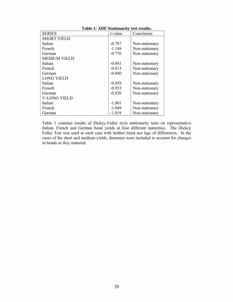
Table 1: ADF Stationarity test results. SERIES t-value Conclusion SHORT YIELD Italian -0.787 Non-stationary French -1.148 Non-stationary German -0.776 Non-stationary MEDIUM YIELD Italian -0.861 Non-stationary French -0.813 Non-stationary German -0.880 Non-stationary LONG YIELD Italian -0.959 Non-stationary French -0.953 Non-stationary German -0.920 Non-stationary V-LONG YIELD Italian -1.001 Non-stationary French -1.049 Non-stationary German -1.019 Non-stationary

Table 1 contains results of Dickey-Fuller style stationarity tests on representative Italian, French and German bond yields at four different maturities. The Dickey Fuller Test was used in each case with neither trend nor lags of differences. In the cases of the short and medium yields, dummies were included to account for changes in bonds as they matured.

30

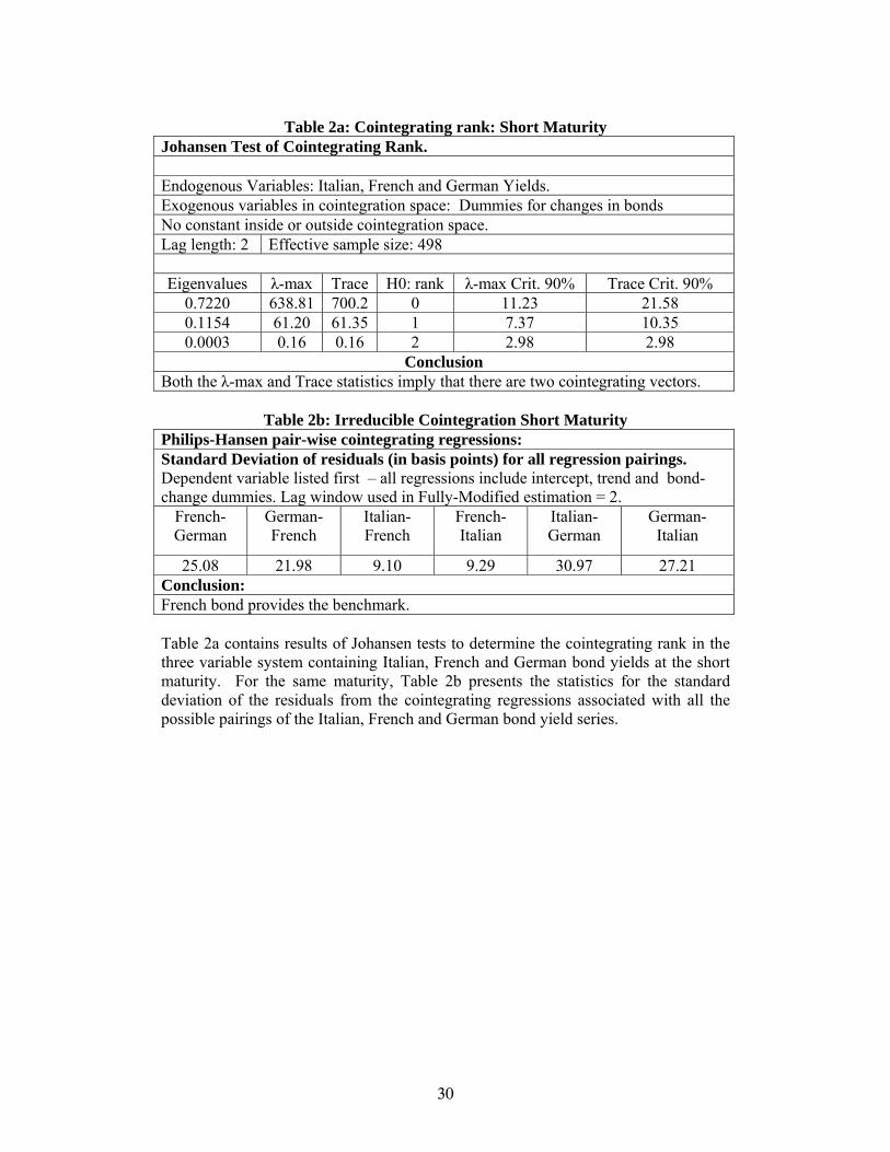
Table 2a: Cointegrating rank: Short Maturity

Johansen Test of Cointegrating Rank. Endogenous Variables: Italian, French and German Yields. Exogenous variables in cointegration space: Dummies for changes in bonds No constant inside or outside cointegration space. Lag length: 2 Effective sample size: 498 Eigenvalues λ-max Trace H0: rank λ-max Crit. 90% Trace Crit. 90%

0.7220 638.81 700.2 0 11.23 21.58 0.1154 61.20 61.35 1 7.37 10.35 0.0003 0.16 0.16 2 2.98 2.98

Conclusion Both the λ-max and Trace statistics imply that there are two cointegrating vectors.

Table 2b: Irreducible Cointegration Short Maturity Philips-Hansen pair-wise cointegrating regressions: Standard Deviation of residuals (in basis points) for all regression pairings. Dependent variable listed first – all regressions include intercept, trend and bond-change dummies. Lag window used in Fully-Modified estimation = 2.

French-German

German-French

Italian-French

French-Italian

Italian-German

German-Italian

25.08 21.98 9.10 9.29 30.97 27.21 Conclusion: French bond provides the benchmark. Table 2a contains results of Johansen tests to determine the cointegrating rank in the three variable system containing Italian, French and German bond yields at the short maturity. For the same maturity, Table 2b presents the statistics for the standard deviation of the residuals from the cointegrating regressions associated with all the possible pairings of the Italian, French and German bond yield series.

31

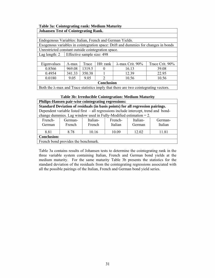
Table 3a: Cointegrating rank: Medium Maturity Johansen Test of Cointegrating Rank. Endogenous Variables: Italian, French and German Yields. Exogenous variables in cointegration space: Drift and dummies for changes in bonds Unrestricted constant outside cointegration space. Lag length: 2 Effective sample size: 498

Eigenvalues Λ-max Trace H0: rank λ-max Crit. 90% Trace Crit. 90% 0.8566 969.08 1319.5 0 16.13 39.08 0.4954 341.33 350.38 1 12.39 22.95 0.0180 9.05 9.05 2 10.56 10.56

Conclusion Both the λ-max and Trace statistics imply that there are two cointegrating vectors.

Table 3b: Irreducible Cointegration: Medium Maturity

Philips-Hansen pair-wise cointegrating regressions: Standard Deviation of residuals (in basis points) for all regression pairings. Dependent variable listed first – all regressions include intercept, trend and bond-change dummies. Lag window used in Fully-Modified estimation = 2.

French-German

German-French

Italian-French

French-Italian

Italian-German

German-Italian

8.81 8.78 10.16 10.09 12.02 11.81 Conclusion: French bond provides the benchmark. Table 3a contains results of Johansen tests to determine the cointegrating rank in the three variable system containing Italian, French and German bond yields at the medium maturity. For the same maturity Table 3b presents the statistics for the standard deviation of the residuals from the cointegrating regressions associated with all the possible pairings of the Italian, French and German bond yield series.

32

Table 4a: Cointegrating rank: Long Maturity Johansen Test of Cointegrating Rank. Endogenous Variables: Italian, French and German Yields. Exogenous variables in cointegration space: Drift. Unrestricted constant outside cointegration space. Lag length: 2 Effective sample size: 498 Eigenvalues λ-max Trace H0: rank λ-max Crit. 90% Trace Crit. 90%

0.0602 30.98 60.44 0 16.13 39.08 0.0511 26.19 29.46 1 12.39 22.95 0.0065 3.27 3.27 2 10.56 10.56

Conclusion Both the λ-max and Trace statistics imply that there are two cointegrating vectors.

Table 4b: Irreducible Cointegration: Long Maturity

Philips-Hansen pair-wise cointegrating regressions: Standard Deviation of residuals (in basis points) for all regression pairings. Dependent variable listed first – all regressions include intercept and trend. There are no bond-changes. Lag window used in Fully-Modified estimation = 2.

French-German

German-French

Italian-French

French-Italian

Italian-German

German-Italian

7.62 7.57 11.83 11.33 13.80 13.13 Conclusion: French bond provides the benchmark. Table 4a contains results of Johansen tests to determine the cointegrating rank in the three variable system containing Italian, French and German bond yields at the long maturity. For the same maturity Table 4b presents the statistics for the standard deviation of the residuals from the cointegrating regressions associated with all the possible pairings of the Italian, French and German bond yield series.

33

Table 5a: Cointegrating rank: Very-Long Maturity

Johansen Test of Cointegrating Rank. Endogenous Variables: Italian, French and German Yields. Exogenous variables in cointegration space: Drift. Unrestricted constant outside cointegration space. Lag length: 2 Effective sample size: 498 Eigenvalues λ-max Trace H0: rank λ-max Crit. 90% Trace Crit. 90%

0.1581 85.72 125.0 0 16.13 39.08 0.0702 36.23 39.27 1 12.39 22.95 0.0061 3.04 3.04 2 10.56 10.56

Conclusion Both the λ-max and Trace statistics imply that there are two cointegrating vectors.

Table 5b: Irreducible Cointegration: Very-Long Maturity

Philips-Hansen pair-wise cointegrating regressions: Standard Deviation of residuals (in basis points) for all regression pairings. Dependent variable listed first – all regressions include intercept and trend. There are no bond-changes. Lag window used in Fully-Modified estimation = 2.

French-German

German-French

Italian-French

French-Italian

Italian-German

German-Italian

7.71 7.62 12.26 11.47 13.16 12.18 Conclusion: Benchmark status is contested between France and Germany Table 5a contains results of Johansen tests to determine the cointegrating rank in the three variable system containing Italian, French and German bond yields at the very-long maturity. For the same maturity Table 5b presents the statistics for the standard deviation of the residuals from the cointegrating regressions associated with all the possible pairings of the Italian, French and German bond yield series.

34

Table 6a: ADF Stationarity Tests Unadjusted Corporate Yields. SERIES t-value Crit. 95% Conclusion 10 year YIELD Maytag -2.276 -2.87 Non-stationary Paper -1.266 -2.87 Non-stationary IBM -1.083 -2.87 Non-stationary

Table 6a contains results of Dickey-Fuller style stationarity tests on corporate bond yields of Maytag Corporation, International Paper and IBM. The (Augmented) Dickey Fuller Test was used in each case without trend but with lags of differences equal to 2, 5 and 0 for Maytag, Paper and IBM respectively. Lags were included until Ljung-Box(Q) statistics were sufficient to reject serial correlation up to the 10th lag with 90% confidence. The number of observations before lags and differences was 412. The ADF critical value for the 95% confidence interval is given for this sample size as it is reported in the Microfit 4.1. econometric software package.

Table 6b: ADF Stationarity Tests Corporate Yields less the Implied Credit Spread. SERIES t-value Crit. 95% Conclusion 10 yr YIELD less credit spread Maytag -1.222 -2.87 Non-stationary Paper -0.825 -2.87 Non-stationary IBM -0.994 -2.87 Non-stationary

Table 6b contains results of Dickey-Fuller style stationarity tests on corporate bond yields adjusted for credit default, of Maytag Corporation, International Paper and IBM. The (Augmented) Dickey Fuller Test was used in each case without trend but with lags of differences equal to 2, 8 and 1 for Maytag, Paper and IBM respectively. Lags were included until Ljung-Box(Q) statistics were sufficient to reject serial correlation up to the 10th lag with 90% confidence. The number of observations before lags and differences was 412. The ADF critical value for the 95% confidence interval is given for this sample size as it is reported in the Microfit 4.1. econometric software package.

35

Table 7a: ADF Stationarity Tests Residuals from Philips-Hansen pair-wise cointegrating regressions. SERIES t-value Crit. 90% Conclusion Regression residual Paper on Maytag (6 ADF lags) -4.566 -3.07 Cointegrated IBM on Maytag (6 ADF lags) -5.492 -3.07 Cointegrated IBM on Paper (7 ADF lags) -3.093 -3.07 Cointegrated

Table 7a contains results of Johansen tests to determine the cointegrating rank in the three variable system containing the corporate yields of Maytag Corporation, International Paper and IBM. The (Augmented) Dickey Fuller Test was used in each case without constant or trend but with lags of differences equal to 2, 8 and 1 for Maytag, Paper and IBM respectively. Lags were included until Ljung-Box(Q) statistics were sufficient to reject serial correlation up to the 10th lag with 90% confidence. The number of observations before lags and differences was 412. The ADF critical value for the 90% confidence interval is given for a sample size of 500 as it is reported in Table B.9 in Hamilton’s (1994) ‘Time Series Analysis’ where we have 2 additional non-stationary right-hand variables in the cointegrating relation12. Table 7b: Corporate Bond Yields at Long Maturity, Irreducible Cointegration Philips-Hansen pair-wise cointegrating regressions: Standard Deviation of residuals for all regression pairings. Dependent variable listed first – all regressions include intercept and CDS of all three corporates. Lag window used in Fully-Modified estimation = 5. IBM-Paper Paper-IBM IBM-Maytag Maytag-IBM Maytag-Paper Paper-Maytag

0.093 0.113 0.140 0.162 0.166 0.175 Conclusion:

IBM bond provides the benchmark. Table 7b presents the statistics for the standard deviation of the residuals from the cointegrating regressions associated with all the possible pairings of the corporate bond yields of Maytag Corporation, International Paper and IBM.

36

Appendix A.

International Paper has significant global businesses in paper, packaging and forest

products. The company has operations in nearly 40 countries, employs approximately

68,700 people worldwide and exports its products to more than 120 nations. Sales of

almost $24 billion annually are derived from businesses located primarily in the

United States, Europe, Latin America, Asia/Pacific and Canada.

Maytag Corporation was a home and commercial appliance company,

headquartered in Newton, Iowa. Sales were $4.7 billion in 2005 and the company had

approximately 18,000 employees worldwide. Maytag was acquired by Whirlpool

Corporation in March, 2006. Whirlpool had sales of more than $19 billion in 2005

and more than 80,000 employees worldwide.

IBM supplies IT hardware, software and Services and is also active in the delivery of

financial services. In 2005 it had revenues of $91.1 billion and 329,373 employees.

37

1 We did in fact carry out Granger-causality tests. The results are generally inconclusive. 2 In what follows, all variables are implicitly indexed by time. To avoid cluttering the notation, we suppress the time subscripts. 3 See for example John Cochrane’s book, ‘Asset Pricing’ (2000). It devotes less than two pages to stationarity. 4 This structure can be motivated in the sovereign bond case as inverse money demand functions with nonstationary velocity.

For example: constant+noisei ir Log vβ= − + where v is the velocity of money. The latter is typically non-

stationary. iβ is the inverse of the interest semi-elasticity of the demand for money and is country-specific.

5 If residuals from the structural vectors are not orthogonal, then it is not clear what ‘structural’ means in this context. It is

essential one way or the other to make some assumption about the covariance between the structural relations. Any assumption

other than a zero value, however, makes the application of the irreducible cointegrating vector approach inconclusive.

6 Short-dated bonds have maturities between 1.25 and 3.5 years. Medium, long and very long bonds have maturity spans of 3.5-

6.5 years, 6.6-13.5 years and >13.5 years respectively. There is also a fifth category for bills: securities with maturity less than

1.25 years. However, until recently, only Italy was significantly trading such instruments on Euro-MTS. 7 It is important to emphasise that we are not claiming that economically yields have unit roots: intuitively one would expect

yields to be mean reverting. Instead, we find statistically that yields are so long-memory that we cannot reject the hypothesis of

non-stationarity.

8 Bowe and Mylonidis (1999) have previously applied the Johansen Procedure to test for integration in European bond markets.

Their work relates to the pre-euro period.

9 CMA stands for Credit Market Analysis Ltd, a London based provider of financial data, see

http://www.creditma.com/products.aspx 10 See Endnote 7 above. 11 For early support of this view, at least at the shorter maturities, see Jessen and Matzen (1999). See also Favero, Pagano and

von Thadden (2005). 12 We found that the IBM CDS implied yield premium was stationary.