Beka 2 Cpt: Two Compartment Model - Loading Dose And ...holford.fmhs.auckland.ac.nz/docs/beka2cpt-lab.pdf · This experiment uses two beakers to simulate a central and a tissue compartment

Nick Holford Page 1 26/09/2017

MEDSCI 719 Pharmacometrics

Beka 2 Cpt: Two Compartment Model - Loading Dose And Maintenance Infusion

Objective

1. To observe the time course of drug concentration in the central and peripheral compartments of a two-compartment system.

2. To compare the time course after 3 types of input:

a. Single Bolus Dose b. Single Bolus Dose and Constant Rate Infusion c. Single Bolus Dose plus First-Order and Constant Rate Infusion

[The inputs studied will depend on student numbers in the course]

Practical Relevance When drugs are administered rapidly and concentrations measured frequently the one-compartment model does not predict the time course of drug concentration very well, especially at early times. This is because it takes time for drug to distribute to the tissues and reach equilibrium. This experiment shows the time course of drug concentration in both central and tissue compartments after a single rapid injection (bolus) with and without a constant rate infusion using a two beaker system to represent a two compartment model. A third method of drug input, the first-order infusion, is added to the Bolus and constant rate infusion to show that it is possible to achieve and maintain a target concentration even when the one-compartment model is not appropriate. The first-order infusion method has been shown to be useful in achieving the target concentration for lignocaine when it is used as an anti-arrhythmic agent.

Organization This experiment is quite demanding in terms of the number of concentration measurements that have to be made. You should have one person responsible for keeping the beakers at their proper levels and taking samples. Another person should be responsible for using the spectrophotometer to measure absorbance and create the calibration curve. The third person should help initially to make sure the others follow the experimental protocol and later on enter the results into the computer and perform the computer analysis.

Method This experiment uses two beakers to simulate a central and a tissue compartment. The central compartment has a nominal volume of 1 L and a clearance of 0.1 l/min. The tissue compartment has a nominal volume of 4 l and an inter-compartmental clearance of 0.4 l/min. Water enters the beakers from a peristaltic pump. These have been carefully set to achieve a flow of 0.1 l/min at a volume of 1 l for the central compartment and 0.4 l/min at a volume of 4 l for the tissue compartment. Water leaves both beakers by overflow. However, you may need to occasionally adjust the flow rate to keep the volume in each container close to the 1 l and 4 l marks. Water enters the central compartment at 0.1 l/min. During the infusion part of the experiment the pump flow is 0.09 l/min and the drip infusion is 0.01 l/min. Before starting the infusion and at its end this pump should be set at 0.1 l/min.

http://www.health.auckland.ac.nz/courses/MEDSCI719/


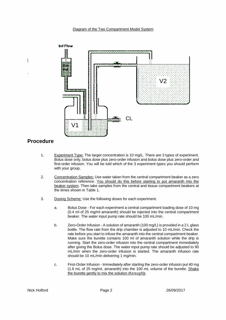
Diagram of the Two Compartment Model System

Experiment The class is divided into groups with one group doing each experiment. There are 3 different experiments: Bolus - A single rapid injection into the central compartment beaker. Bolus+Zero-Order Infusion - A rapid injection is given into the central compartment followed

immediately by starting a constant rate (zero-order) infusion. Bolus+Zero-Order+First-Order Infusion - A rapid injection and constant rate (zero-order) infusion

are given into the central compartment. A loading dose sufficient to fill the tissue compartment (larger beaker) is put into the burette of the giving set. The flow rate through the burette and its volume determine the first-order input rate. As the drip continues it slowly dilutes the solution in the burette and the rate at which drug enters the central compartment decreases until eventually the concentration in the burette is the same as that in the plastic bag providing the solution for the constant rate (zero-order) infusion.

Procedure

1. Experiment Type: The target concentration is 10 mg/L. There are 3 types of experiment. Bolus dose only, bolus dose plus zero-order infusion and bolus dose plus zero-order and first-order infusion. You will be told which of the 3 experiment types you should perform with your group.

2. Concentration Samples: Use water taken from the central compartment beaker as a zero concentration reference. You should do this before starting to put amaranth into the beaker system. Then take samples from the central and tissue compartment beakers at the times shown in Table 1.

3. Dosing Scheme: Use the following doses for each experiment.

a. Bolus Dose - For each experiment a central compartment loading dose of 10 mg

(0.4 ml of 25 mg/ml amaranth) should be injected into the central compartment beaker. The water input pump rate should be 100 mL/min.

b. Zero-Order Infusion - A solution of amaranth (100 mg/L) is provided in a 2 L glass

bottle. The flow rate from the drip chamber is adjusted to 10 mL/min. Check the rate before you start to infuse the amaranth into the central compartment beaker. Make sure the burette contains 100 ml of amaranth solution while the drip is running. Start the zero-order infusion into the central compartment immediately after giving the Bolus dose. The water input pump rate should be adjusted to 90 mL/min when the zero-order infusion is started. The amaranth infusion rate should be 10 mL/min delivering 1 mg/min.

c. First-Order Infusion - Immediately after starting the zero-order infusion put 40 mg

(1.6 mL of 25 mg/mL amaranth) into the 100 mL volume of the burette. Shake the burette gently to mix the solution thoroughly.

CL

V2

V1


4. Calibration Curve: The spectrophotometer is set for absorbance at 518 nm. Zero the

spectrophotometer with the blank sample taken from the central compartment beaker before any dose was administered. Calibrate the spectrophotometer using the amaranth standard solutions (0.1, 0.5, 2, 5, 10, 20, 25 mg/L).

a. Plot a graph of amaranth standard concentration versus absorbance using the results from the first set of measurements of concentration standards.

b. Draw a best fit line through the points using Excel (should you force the line through zero?).

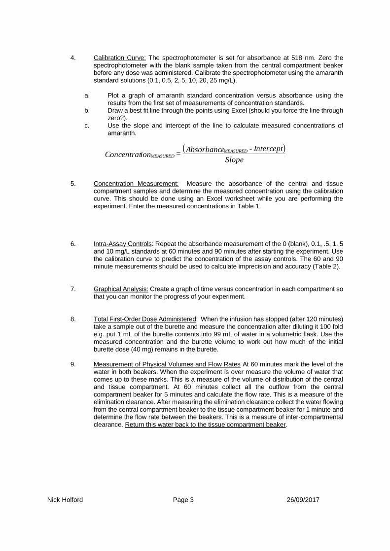
c. Use the slope and intercept of the line to calculate measured concentrations of amaranth.

5. Concentration Measurement: Measure the absorbance of the central and tissue

compartment samples and determine the measured concentration using the calibration curve. This should be done using an Excel worksheet while you are performing the experiment. Enter the measured concentrations in Table 1.

6. Intra-Assay Controls: Repeat the absorbance measurement of the 0 (blank), 0.1, .5, 1, 5 and 10 mg/L standards at 60 minutes and 90 minutes after starting the experiment. Use the calibration curve to predict the concentration of the assay controls. The 60 and 90 minute measurements should be used to calculate imprecision and accuracy (Table 2).

7. Graphical Analysis: Create a graph of time versus concentration in each compartment so that you can monitor the progress of your experiment.

8. Total First-Order Dose Administered: When the infusion has stopped (after 120 minutes)

take a sample out of the burette and measure the concentration after diluting it 100 fold e.g. put 1 mL of the burette contents into 99 mL of water in a volumetric flask. Use the measured concentration and the burette volume to work out how much of the initial burette dose (40 mg) remains in the burette.

9. Measurement of Physical Volumes and Flow Rates At 60 minutes mark the level of the water in both beakers. When the experiment is over measure the volume of water that comes up to these marks. This is a measure of the volume of distribution of the central and tissue compartment. At 60 minutes collect all the outflow from the central compartment beaker for 5 minutes and calculate the flow rate. This is a measure of the elimination clearance. After measuring the elimination clearance collect the water flowing from the central compartment beaker to the tissue compartment beaker for 1 minute and determine the flow rate between the beakers. This is a measure of inter-compartmental clearance. Return this water back to the tissue compartment beaker.

Slope

Intercept - Absorbance = ionConcentrat

MEASUREDMEASURED


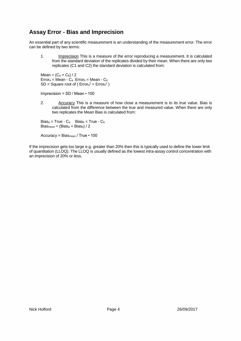
Assay Error - Bias and Imprecision An essential part of any scientific measurement is an understanding of the measurement error. The error can be defined by two terms:

1. Imprecision This is a measure of the error reproducing a measurement. It is calculated from the standard deviation of the replicates divided by their mean. When there are only two replicates (C1 and C2) the standard deviation is calculated from:

Mean = (Ca + Cb) / 2 Errora = Mean - Ca Errorb = Mean - Cb SD = Square root of ( Errora

2 + Errorb2 )

Imprecision = SD / Mean • 100

2. Accuracy This is a measure of how close a measurement is to its true value. Bias is calculated from the difference between the true and measured value. When there are only two replicates the Mean Bias is calculated from:

Biasa = True - Ca Biasb = True - Cb Biasmean = (Biasa + Biasb) / 2 Accuracy = Biasmean / True • 100

If the imprecision gets too large e.g. greater than 20% then this is typically used to define the lower limit of quantitation (LLOQ). The LLOQ is usually defined as the lowest intra-assay control concentration with an imprecision of 20% or less.


Data Entry and Analysis You may choose to analyse the results using Monolix or NONMEM. NONMEM may be quicker and more reliable but you will have to construct graphs using Excel.

Monolix 1. Monolix Data: Create an Excel worksheet to enter the time and concentration data. The

first column of the worksheet should be named #ID, the second DVID, the third TIME, the fourth DV and the fifth AMT. Enter the value 1 in all rows of the #ID column. The central compartment times and concentrations should be entered first and have the number 1 in the DVID column. Do not enter values at time 0. The tissue compartment times and concentrations should be entered beneath the central compartment values and have the number 2 in the DVID column

2. Enter 0 in every row of the AMT column (this is to workaround a Monolix bug). 3. IMPORTANT: After entering the data sort the worksheet on TIME.

4. Save the worksheet in CSV format with the name “beka.csv” 5. Open Monolix and create a new project

. 6. Save it in My Pharmacometrics\Pharmacometrics Data\BEKA 2 Cpt Experiment with the

name “beka_project”. 7. Click on “The data” and select your beka.csv file 8. Monolix should identify the columns as “ID”, “YTYPE”, “TIME”, “Y”,"AMT" 9. Accept the data 10. Click on “The Structural Model” 11. Click on “Other list” and select the beka_mlxt model from the My

Pharmacometrics\Pharmacometrics Data\BEKA 2 Cpt Experiment folder 12. Click on “Compile” and “Accept” 13. Click all the “1” values in the covariance model block so that they become “0”. This should

gray out the values in the “Stand. Dev.of the random effects” box. 14. Choose the “comb2” residual error model for both types of observation (Central and

peripheral compartment concs) 15. Enter initial estimates for CL (0.1 L/min), VC (1 L), CLic (0.4 L/min) and VT (4 L) in the

“Fixed effects” box. 16. Enter 0.01 for the additive error parameter (“a”) and 0.1 for the proportional error

parameter (“b”) in the “Residual error parameters” box. 17. Save the project. 18. Run the model to estimate the Population parameters 19. Create VPCs for the Central and Tissue compartment observations.

.

NONMEM

1. NONMEM Data: Create an Excel worksheet to enter the time and concentration data. The first column of the worksheet should be named #ID, the second DVID, the third TIME, the fourth DV. Enter the value 1 in all rows of the #ID column. The central compartment times and concentrations should be entered in time sequence. Put the number 1 in the DVID column for central compartment and number 2 in the DVID column for the tissue compartment. Do not enter values at time 0.

2. IMPORTANT: After entering the data sort the worksheet on TIME. 3. Save the worksheet in CSV format with the name “beka.csv” 4. Open a NONMEM window.

. 5. Change directory to My Pharmacometrics\Pharmacometrics Data\BEKA 2 Cpt

Experiment. 6. Run the model to estimate the Population parameters with this command:


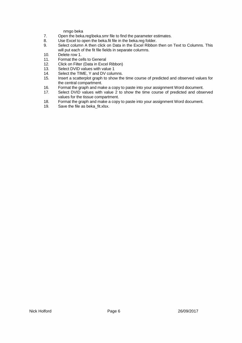
nmgo beka 7. Open the beka.reg\beka.smr file to find the parameter estimates. 8. Use Excel to open the beka.fit file in the beka.reg folder. 9. Select column A then click on Data in the Excel Ribbon then on Text to Columns. This

will put each of the fit file fields in separate columns. 10. Delete row 1. 11. Format the cells to General 12. Click on Filter (Data in Excel Ribbon) 13. Select DVID values with value 1 14. Select the TIME, Y and DV columns. 15. Insert a scatterplot graph to show the time course of predicted and observed values for

the central compartment. 16. Format the graph and make a copy to paste into your assignment Word document. 17. Select DVID values with value 2 to show the time course of predicted and observed

values for the tissue compartment. 18. Format the graph and make a copy to paste into your assignment Word document. 19. Save the file as beka_fit.xlsx.


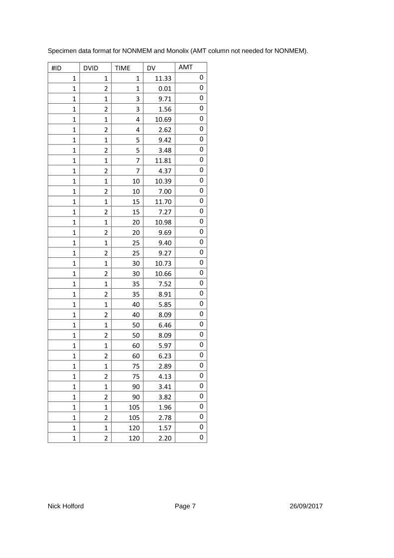
Specimen data format for NONMEM and Monolix (AMT column not needed for NONMEM).

#ID DVID TIME DV AMT

1 1 1 11.33 0

1 2 1 0.01 0

1 1 3 9.71 0

1 2 3 1.56 0

1 1 4 10.69 0

1 2 4 2.62 0

1 1 5 9.42 0

1 2 5 3.48 0

1 1 7 11.81 0

1 2 7 4.37 0

1 1 10 10.39 0

1 2 10 7.00 0

1 1 15 11.70 0

1 2 15 7.27 0

1 1 20 10.98 0

1 2 20 9.69 0

1 1 25 9.40 0

1 2 25 9.27 0

1 1 30 10.73 0

1 2 30 10.66 0

1 1 35 7.52 0

1 2 35 8.91 0

1 1 40 5.85 0

1 2 40 8.09 0

1 1 50 6.46 0

1 2 50 8.09 0

1 1 60 5.97 0

1 2 60 6.23 0

1 1 75 2.89 0

1 2 75 4.13 0

1 1 90 3.41 0

1 2 90 3.82 0

1 1 105 1.96 0

1 2 105 2.78 0

1 1 120 1.57 0

1 2 120 2.20 0


Graphical Analysis

1. Using Excel plot a graph of the measured concentrations for central and tissue compartments against time. Obtain a copy of this graph from other groups so that you can see the pattern for each of the dosing experiments.

2. Bolus dose only experiment:

a. Calculate the half-life from the both the central and tissue compartment concentrations measured from 60 minutes onwards.

b. Calculate the AUCinf from the measured central compartment concentrations using the trapezoidal rule. Derive the Clearance from the total dose administered and AUCinf.

3. Steady state infusion experiments: a. Estimate the steady state concentration. Derive the Clearance from the infusion rate and the

steady state concentration.


Assignment Your assignment should include the following results: 1. Calibration curve graph 2. Table 1 TWO COMPARTMENT OBSERVATIONS

3. Table 2 ASSAY ERROR

4. Table 3 TWO COMPARTMENT PARAMETER ESTIMATES 5. Graph of the measured concentrations (linear and log scales) 6. Graph showing the computer fit to the data 7. Table of Monolix and/or NONMEM parameter estimates 8. Beka model (Monolix or NONMEM) 9. Answers to the following questions:

9.1. What are potential sources of error in the calibration curve? How can these be reduced or allowed for?

9.2. What are the sources of error in the intra-assay control measurements? Why are intra-assay controls used?

9.3. Briefly describe the beka model (Monolix or NONMEM) used to estimate the parameters. 9.4. Compare the clearance estimates from the graphical (AUCinf method or steady state conc) and

the computer model predictions. Discuss why there might be differences between the clearance estimated by the two methods.

9.5. Using the data obtained from the bolus dose experiment: 9.5.1. How does the half-life calculated from 60 minutes onwards using the central compartment

concentrations compare with the half-life calculated from 0.7 • Vd/CL? Why are they different?

9.5.2. How does the half-life estimated from the central compartment concentrations compare to that estimated from the tissue compartment concentrations? Should they be the same or different? Explain your answer.

9.5.3. Calculate the tissue compartment half-life from 0.7 * V2/CLic and the burette half-life from 0.7 • Burette Volume/Drip Flow Rate. They should be similar.

9.6. If V2 was known to be 6000 mL what loading dose is required in the burette for the first-order infusion?

9.7. If V2 was known to be 6000 mL what other change to the dose administration system would be needed to achieve and maintain a target concentration of 10 mg/l?


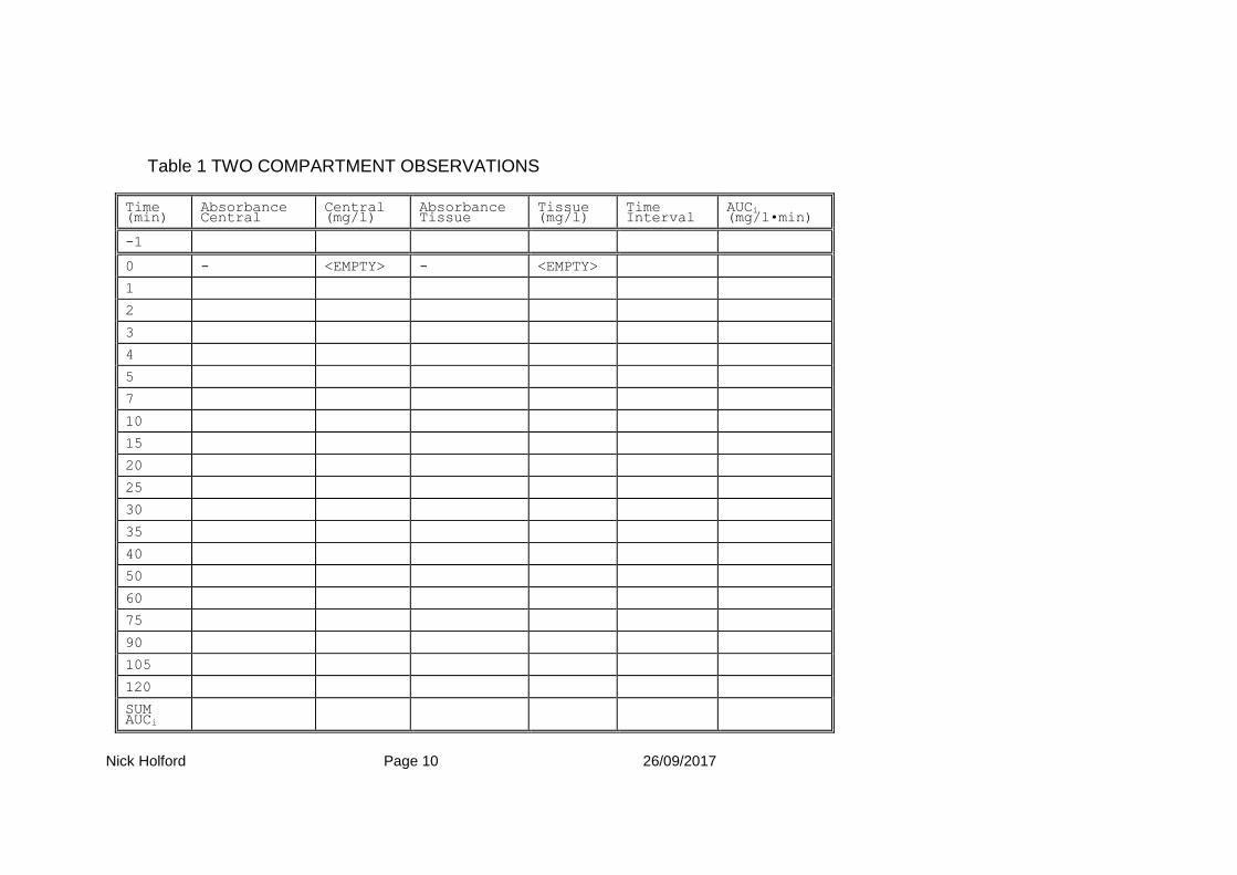
Table 1 TWO COMPARTMENT OBSERVATIONS

Time (min)

Absorbance Central

Central (mg/l)

Absorbance Tissue

Tissue (mg/l)

Time Interval

AUCi (mg/l•min)

-1

0 - <EMPTY> - <EMPTY>

1

2

3

4

5

7

10

15

20

25

30

35

40

50

60

75

90

105

120

SUM AUCi


Table 2 ASSAY ERROR

True Conc (mg/l)

Absorbance Replicates

Conc (mg/l)

Mean Error (Mean -

True Conc)

SD Accuracy % Imprecision %

0 a.

b.

a.

b.

a.

b.

0.1 a.

b.

a.

b.

a.

b.

0.5 a.

b.

a.

b.

a.

b.

1.0 a.

b.

a.

b.

a.

b.

5.0 a.

b.

a.

b.

a.

b.

10.0 a.

b.

a.

b.

a.

b.

a. = 60 minute intra-assay control b. = 90 minute intra-assay control


Table 3 TWO COMPARTMENT PARAMETER ESTIMATES

Parameter Name Method Value

Vc (Central Beaker)

Measured

CL (Central exit flow rate)

Measured

Vt (Tissue Beaker)

Measured

CLic (Tissue exit flow rate)

Measured

T½ Central Graph (bolus experiment)

T½ Tissue Graph (bolus experiment)

T½ .7•Vc/CL Computer

AUCTlast Graph (bolus experiment)

AUCextrap Graph (bolus experiment)

AUCinf Graph (bolus experiment)

CL Graph (steady state infusion experiments)

Vc Computer

CL Computer

Vt Computer

CLic Computer

Additive error Central (“a”)

Computer

Proportional error Central (“b”)

Computer

Additive error Tissue (“a”)

Computer

Proportional error Tissue (“a”)

Computer

MQC Calibration Curve

Documents

Beka 2 Cpt: Two Compartment Model - Loading Dose And ...holford.fmhs.auckland.ac.nz/docs/beka2cpt-lab.pdf · This experiment uses two beakers to simulate a central and a tissue compartment