Embed Size (px)
Citation preview
V. A. F. CostaDepartamento de Engenharia Mecânica da
Universidade de Aveiro,Campus Universitário de Santiago,
3810-193 Aveiro, Portugale-mail: v�[email protected]
Bejan’s Heatlines and Masslinesfor Convection Visualization andAnalysisHeatlines were proposed in 1983 by Kimura and Bejan (1983) as adequate tools forvisualization and analysis of convection heat transfer. The masslines, their equivalent toapply to convection mass transfer, were proposed in 1987 by Trevisan and Bejan. Thesevisualization and analysis tools proved to be useful, and their application in the fields ofconvective heat and/or mass transfer is still increasing. When the heat function and/or themass function are made dimensionless in an adequate way, their values are closelyrelated with the Nusselt and/or Sherwood numbers. The basics of the method were es-tablished in the 1980(s), and some novelties were subsequently added in order to increasethe applicability range and facility of use of such visualization tools. Main steps includedtheir use in unsteady problems, their use in polar cylindrical and spherical coordinatesystems, development of similarity expressions for the heat function in laminar convectiveboundary layers, application of the method to turbulent flow problems, unification of thestreamline, heatline, and massline methods (involving isotropic or anisotropic media),and the extension and unification of the method to apply to reacting flows. The method isnow well established, and the efforts made towards unification resulted in very usefultools for visualization and analysis, which can be easily included in software packagesfor numerical heat transfer and fluid flow. This review describes the origins and evolutionof the heatlines and masslines as visualization and analysis tools, from their first steps tothe present. �DOI: 10.1115/1.2177684�
1 Introduction
When dealing with fluid flow, streamlines are well establishedas the most adequate and very useful tools to visualize two-dimensional incompressible flows from a long time ago �cf. �1��,and they are present in virtually any study or textbook on fluiddynamics. In a way similar to the streamlines, the heat flux linesare well established to visualize two-dimensional conductive heattransfer in isotropic media �2�. In this case, the heat flux lines arenormal to the isotherms, and each one can be easily obtained fromthe other, and both are routinely used when dealing with conduc-tive heat transfer.
When dealing with convective heat transfer, the isotherms arenot the most adequate tools for visualization and analysis, and theheat flux lines are not necessarily perpendicular to them. Takeninto consideration the total energy flux �enthalpy advection andheat diffusion�, the heat flux lines, referred to as the heatlines, canalso apply. The heat function and heatline concepts and formula-tion were originally introduced by Kimura and Bejan �3� in the1980�s�, and they appeared for the first time in a book on convec-tive heat transfer by Bejan in 1984 �4�. Before that, convectiveheat transfer processes were analyzed using mainly the isotherms.But, the adequate visualizing tools in fluid dynamics are thestreamlines and not the isobars, the same occurring in the field ofconvective heat transfer, where the adequate visualizing tools arethe heatlines and not the isotherms.
A natural extension of the method was made to the field ofconvective mass transfer, through the introduction of the massfunction and massline concepts by Trevisan and Bejan �5� in1987.
If the heat function and/or the mass function are made dimen-sionless in an adequate way, their numerical values are closelyrelated to the overall Nusselt and/or Sherwood numbers. In this
Transmitted by Assoc. Editor E. Dowell.
126 / Vol. 59, MAY 2006 Copyright © 200
way, they are very useful tools not only for visualization purposesbut also for the analysis of the overall heat and/or mass transferprocesses.
Once established the heatlines and masslines have been used asvisualization and analysis tools of many and varied convectiveheat and mass transfer problems �3,5–13�. Some studies using theheatlines include thermomagnetic convection in electroconductivemelts �14,15�. The heatline concept was also used for visualizationand analysis of unsteady convective heat transfer, assuming that,at a given instant of analysis, the steady state version of the energyconservation equation is satisfied, as set forth by Aggarwal andManhapra �16,17�.
Application of the method to polar cylindrical coordinate sys-tems was made firstly by Littlefield and Desai �18� to study thenatural convection in a vertical cylindrical annulus, and later ap-plied to some convection problems in circular annuli �19–21�. Inthe referred studies, the visualization using the heatlines is madein the r-� plane �19,20�, or in the r-z plane �18,21�. The methodwas also applied to polar spherical coordinate systems by Chatto-padhyay and Dash �22�, using the r-� plane for visualization ofthe heatlines, where � is the azimuthal angle.
The heatlines were also applied to some forced convectionboundary layers, both in open �23� or fluid-saturated porous media�24�, by developing the similarity expressions for the heatfunctioncorresponding to different heating or cooling wall conditions.Similarity expressions for the heat function were also obtained forlaminar natural convection boundary layers adjacent to a verticalwall, considering different heating or cooling wall conditions �25�.
The heatline concept was also applied when dealing with heattransfer in turbulent flows through the consideration of the turbu-lent fluxes into the heat function differential equation �26�. If theheat transfer problem under analysis occurs in the turbulentboundary layer near a wall, the heatline concept can be applied ina simpler way, by using an effective diffusion coefficient for heat,which includes the eddy diffusivity effect of the turbulent trans-port �27�.
The heatline and massline methods evolved in a natural way,
6 by ASME Transactions of the ASME
and they appeared in a mature form in convection books, both inopen fluid domains �27,28� and in porous domains �29�. In therecent book on convection heat transfer by Bejan �28�, the methodis used extensively. Once the method was established, some nov-elties were introduced in order to enlarge its applicability rangeand to ease its inclusion into computational fluid dynamics �CFD�codes and packages. The unification of the streamline, heatline,and massline methods, which are treated in a common way, wasmade by Costa �30�, thus resulting in a general tool that can beeasily included in CFD software codes and packages. This in-cludes, for the first time, the possibility of variable diffusion co-efficient for the function used for visualization purposes. Somecontroversy was associated with the treatment of such diffusioncoefficients �10�, but the adequate treatment is now well estab-lished �31�. The unified version of the streamline, heatline, andmassline methods to apply to convective heat and mass transfer inanisotropic fluid-saturated porous media was also derived byCosta �32�, which is of crucial importance when dealing withmany natural or manufactured products, and it is a valuable toolthat can be easily included in CFD codes and packages.
The last remarkable improvement of the method was made inorder to apply it to reacting flows. As the method applies todivergence-free problems, special care should be taken when se-lecting the conserved variables to consider, without source termsin the governing differential equations. This was done by Mukho-padhyay et al. �33,34�, by selecting as variables the normalizedelemental mass fractions and the total enthalpy �formation en-thalpy plus sensible enthalpy�, with very encouraging results.
In what follows, presentation is made of the author’s vision onthe most important issues related with the development and appli-cation of the heatline and massline methods, and some illustrativeexamples of their application are also presented. A visit is made tothe references involving the heatlines and masslines, both in whatconcerns new developments of the method or just its application.This is a work started before by Costa �35�, but that, fortunately,needs to always be updated.
2 Origins of the Heat Function and Heatlines
2.1 Stream Function and Streamlines. The stream functionand the streamlines are very useful tools when dealing with 2Dfluid flow visualization and analysis, or even when dealing with2D fluid flow calculations using a vorticity-stream functionformulation.
For such situations, the mass conservation equation for an in-compressible fluid reads
�
�x��u� +
�
�y��v� = 0 �1�
Noting that �u and �v are the mass fluxes in the x and y direc-tions, respectively, the stream function ��x ,y� can be introducedand defined through its first-order derivatives as
��
�y= Jm,x = �u �2a�
−��
�x= Jm,y = �v �2b�
Equation �1� is identically obtained evaluating and invoking theequality of the second-order crossed derivatives of ��x ,y�.
The differential of the stream function ��x ,y� can be expressedas
d� =��
�xdx +
��
�ydy = − Jm,ydx + Jm,xdy �3�
or
Applied Mechanics Reviews
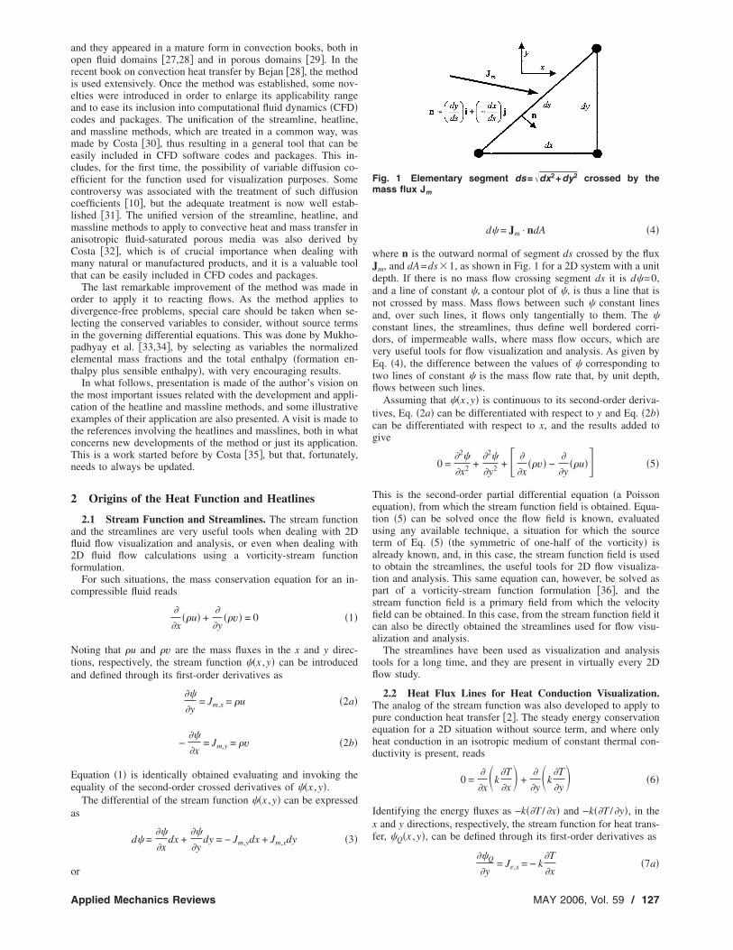
d� = Jm · ndA �4�
where n is the outward normal of segment ds crossed by the fluxJm, and dA=ds�1, as shown in Fig. 1 for a 2D system with a unitdepth. If there is no mass flow crossing segment ds it is d�=0,and a line of constant �, a contour plot of �, is thus a line that isnot crossed by mass. Mass flows between such � constant linesand, over such lines, it flows only tangentially to them. The �constant lines, the streamlines, thus define well bordered corri-dors, of impermeable walls, where mass flow occurs, which arevery useful tools for flow visualization and analysis. As given byEq. �4�, the difference between the values of � corresponding totwo lines of constant � is the mass flow rate that, by unit depth,flows between such lines.
Assuming that ��x ,y� is continuous to its second-order deriva-tives, Eq. �2a� can be differentiated with respect to y and Eq. �2b�can be differentiated with respect to x, and the results added togive
0 =�2�
�x2 +�2�
�y2 + � �
�x��v� −
�
�y��u�� �5�
This is the second-order partial differential equation �a Poissonequation�, from which the stream function field is obtained. Equa-tion �5� can be solved once the flow field is known, evaluatedusing any available technique, a situation for which the sourceterm of Eq. �5� �the symmetric of one-half of the vorticity� isalready known, and, in this case, the stream function field is usedto obtain the streamlines, the useful tools for 2D flow visualiza-tion and analysis. This same equation can, however, be solved aspart of a vorticity-stream function formulation �36�, and thestream function field is a primary field from which the velocityfield can be obtained. In this case, from the stream function field itcan also be directly obtained the streamlines used for flow visu-alization and analysis.
The streamlines have been used as visualization and analysistools for a long time, and they are present in virtually every 2Dflow study.
2.2 Heat Flux Lines for Heat Conduction Visualization.The analog of the stream function was also developed to apply topure conduction heat transfer �2�. The steady energy conservationequation for a 2D situation without source term, and where onlyheat conduction in an isotropic medium of constant thermal con-ductivity is present, reads
0 =�
�x�k
�T
�x� +
�
�y�k
�T
�y� �6�
Identifying the energy fluxes as −k��T /�x� and −k��T /�y�, in thex and y directions, respectively, the stream function for heat trans-fer, �Q�x ,y�, can be defined through its first-order derivatives as
��Q = Je,x = − k�T
�7a�
Fig. 1 Elementary segment ds=dx2+dy2 crossed by themass flux Jm
�y �x
MAY 2006, Vol. 59 / 127
−��Q
�x= Je,y = − k
�T
�y�7b�
Equation �6� is identically obtained by adding the second-ordermixed derivatives of �Q�x ,y�.
Assuming that �Q�x ,y� is continuous to its second-order deriva-tives, Eq. �7a� can be differentiated with respect to y and Eq. �7b�can be differentiated with respect to x, and the obtained resultsadded to give
0 =�2�Q
�x2 +�2�Q
�y2 �8�
From this Laplace equation one obtains the �Q�x ,y� field and,from it, the heat flux lines for visualization and analysis. Heatflows in such a way that the constant �Q�x ,y� lines, the contourplots of �Q�x ,y�, are not crossed by heat.
For an isotropic medium of constant thermal conductivity, tak-ing Eqs. �7a� and �7b�, it is
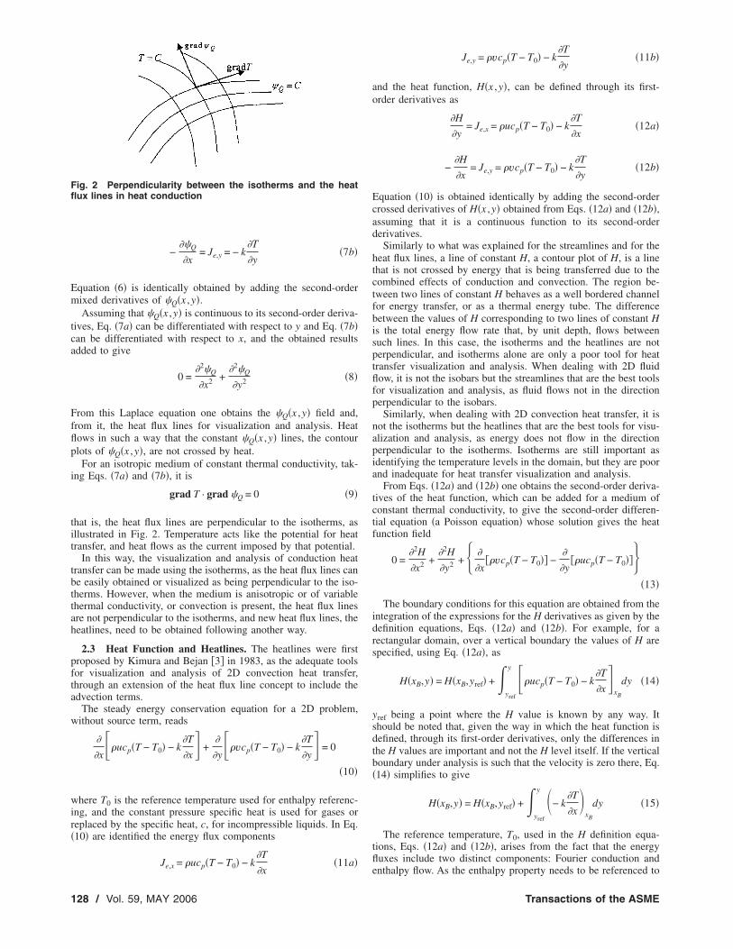
grad T · grad �Q = 0 �9�
that is, the heat flux lines are perpendicular to the isotherms, asillustrated in Fig. 2. Temperature acts like the potential for heattransfer, and heat flows as the current imposed by that potential.
In this way, the visualization and analysis of conduction heattransfer can be made using the isotherms, as the heat flux lines canbe easily obtained or visualized as being perpendicular to the iso-therms. However, when the medium is anisotropic or of variablethermal conductivity, or convection is present, the heat flux linesare not perpendicular to the isotherms, and new heat flux lines, theheatlines, need to be obtained following another way.
2.3 Heat Function and Heatlines. The heatlines were firstproposed by Kimura and Bejan �3� in 1983, as the adequate toolsfor visualization and analysis of 2D convection heat transfer,through an extension of the heat flux line concept to include theadvection terms.
The steady energy conservation equation for a 2D problem,without source term, reads
�
�x��ucp�T − T0� − k
�T
�x� +
�
�y��vcp�T − T0� − k
�T
�y� = 0
�10�
where T0 is the reference temperature used for enthalpy referenc-ing, and the constant pressure specific heat is used for gases orreplaced by the specific heat, c, for incompressible liquids. In Eq.�10� are identified the energy flux components
Je,x = �ucp�T − T0� − k�T
�11a�
Fig. 2 Perpendicularity between the isotherms and the heatflux lines in heat conduction
�x
128 / Vol. 59, MAY 2006
Je,y = �vcp�T − T0� − k�T
�y�11b�
and the heat function, H�x ,y�, can be defined through its first-order derivatives as
�H
�y= Je,x = �ucp�T − T0� − k
�T
�x�12a�
−�H
�x= Je,y = �vcp�T − T0� − k
�T
�y�12b�
Equation �10� is obtained identically by adding the second-ordercrossed derivatives of H�x ,y� obtained from Eqs. �12a� and �12b�,assuming that it is a continuous function to its second-orderderivatives.
Similarly to what was explained for the streamlines and for theheat flux lines, a line of constant H, a contour plot of H, is a linethat is not crossed by energy that is being transferred due to thecombined effects of conduction and convection. The region be-tween two lines of constant H behaves as a well bordered channelfor energy transfer, or as a thermal energy tube. The differencebetween the values of H corresponding to two lines of constant His the total energy flow rate that, by unit depth, flows betweensuch lines. In this case, the isotherms and the heatlines are notperpendicular, and isotherms alone are only a poor tool for heattransfer visualization and analysis. When dealing with 2D fluidflow, it is not the isobars but the streamlines that are the best toolsfor visualization and analysis, as fluid flows not in the directionperpendicular to the isobars.
Similarly, when dealing with 2D convection heat transfer, it isnot the isotherms but the heatlines that are the best tools for visu-alization and analysis, as energy does not flow in the directionperpendicular to the isotherms. Isotherms are still important asidentifying the temperature levels in the domain, but they are poorand inadequate for heat transfer visualization and analysis.
From Eqs. �12a� and �12b� one obtains the second-order deriva-tives of the heat function, which can be added for a medium ofconstant thermal conductivity, to give the second-order differen-tial equation �a Poisson equation� whose solution gives the heatfunction field
0 =�2H
�x2 +�2H
�y2 + �
�x��vcp�T − T0�� −
�
�y��ucp�T − T0���
�13�
The boundary conditions for this equation are obtained from theintegration of the expressions for the H derivatives as given by thedefinition equations, Eqs. �12a� and �12b�. For example, for arectangular domain, over a vertical boundary the values of H arespecified, using Eq. �12a�, as
H�xB,y� = H�xB,yref� +�yref
y ��ucp�T − T0� − k�T
�x�
xB
dy �14�
yref being a point where the H value is known by any way. Itshould be noted that, given the way in which the heat function isdefined, through its first-order derivatives, only the differences inthe H values are important and not the H level itself. If the verticalboundary under analysis is such that the velocity is zero there, Eq.�14� simplifies to give
H�xB,y� = H�xB,yref� +�yref
y �− k�T
�x�
xB
dy �15�
The reference temperature, T0, used in the H definition equa-tions, Eqs. �12a� and �12b�, arises from the fact that the energyfluxes include two distinct components: Fourier conduction and
enthalpy flow. As the enthalpy property needs to be referenced toTransactions of the ASME
a given state, this is chosen as the one corresponding to tempera-ture T0. Selection of T0 is arbitrary, but it has an influence on theobtained heatlines, given that different values of T0 lead to differ-ent slopes of the H field, as given by Eqs. �12a� and �12b�. Thevalue of T0 is irrelevant in what concerns the energy conservationequation; once invoked the mass conservation equation, the termsinvolving T0 vanish in the energy conservation equation. This isdifferent, however, in the differential equation governing the Hfield, Eq. �13�, whose source term depends on T0. In order to solvethis problem, a unified treatment has been proposed by Bejan �27�,by setting T0 as the minimum temperature level in the domainunder analysis.
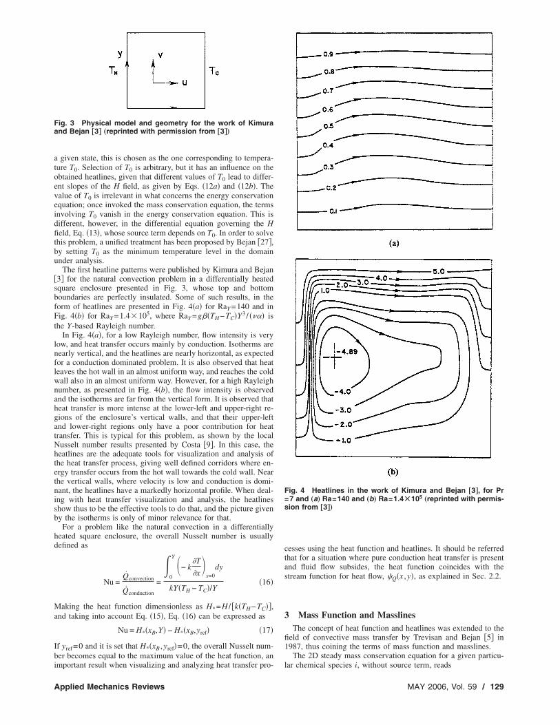
The first heatline patterns were published by Kimura and Bejan�3� for the natural convection problem in a differentially heatedsquare enclosure presented in Fig. 3, whose top and bottomboundaries are perfectly insulated. Some of such results, in theform of heatlines are presented in Fig. 4�a� for RaY =140 and inFig. 4�b� for RaY =1.4�105, where RaY =g��TH−TC�Y3 / ���� isthe Y-based Rayleigh number.
In Fig. 4�a�, for a low Rayleigh number, flow intensity is verylow, and heat transfer occurs mainly by conduction. Isotherms arenearly vertical, and the heatlines are nearly horizontal, as expectedfor a conduction dominated problem. It is also observed that heatleaves the hot wall in an almost uniform way, and reaches the coldwall also in an almost uniform way. However, for a high Rayleighnumber, as presented in Fig. 4�b�, the flow intensity is observedand the isotherms are far from the vertical form. It is observed thatheat transfer is more intense at the lower-left and upper-right re-gions of the enclosure’s vertical walls, and that their upper-leftand lower-right regions only have a poor contribution for heattransfer. This is typical for this problem, as shown by the localNusselt number results presented by Costa �9�. In this case, theheatlines are the adequate tools for visualization and analysis ofthe heat transfer process, giving well defined corridors where en-ergy transfer occurs from the hot wall towards the cold wall. Nearthe vertical walls, where velocity is low and conduction is domi-nant, the heatlines have a markedly horizontal profile. When deal-ing with heat transfer visualization and analysis, the heatlinesshow thus to be the effective tools to do that, and the picture givenby the isotherms is only of minor relevance for that.
For a problem like the natural convection in a differentiallyheated square enclosure, the overall Nusselt number is usuallydefined as
Nu =Qconvection
Qconduction
=
�0
Y �− k�T
�x�
x=0dy
kY�TH − TC�/Y�16�
Making the heat function dimensionless as H*=H / �k�TH−TC��,and taking into account Eq. �15�, Eq. �16� can be expressed as
Nu = H*�xB,Y� − H*�xB,yref� �17�
If yref=0 and it is set that H*�xB ,yref�=0, the overall Nusselt num-ber becomes equal to the maximum value of the heat function, an
Fig. 3 Physical model and geometry for the work of Kimuraand Bejan †3‡ „reprinted with permission from †3‡…
important result when visualizing and analyzing heat transfer pro-
Applied Mechanics Reviews
cesses using the heat function and heatlines. It should be referredthat for a situation where pure conduction heat transfer is presentand fluid flow subsides, the heat function coincides with thestream function for heat flow, �Q�x ,y�, as explained in Sec. 2.2.
3 Mass Function and MasslinesThe concept of heat function and heatlines was extended to the
field of convective mass transfer by Trevisan and Bejan �5� in1987, thus coining the terms of mass function and masslines.
The 2D steady mass conservation equation for a given particu-
Fig. 4 Heatlines in the work of Kimura and Bejan †3‡, for Pr=7 and „a… Ra=140 and „b… Ra=1.4Ã105
„reprinted with permis-sion from †3‡…
lar chemical species i, without source term, reads
MAY 2006, Vol. 59 / 129
�
�x��u�Ci − Ci,0� − �Di
�Ci
�x� +
�
�y��v�Ci − Ci,0� − �Di
�Ci
�y� = 0
�18�
where Ci,0 is the minimum value of the mass concentration ofcomponent i, similarly to what was made for the reference tem-perature T0 in Eq. �10�. Identifying the mass flux components ofspecies i as
Jmi,x= �u�Ci − Ci,0� − �Di
�Ci
�x�19a�
Jmi,y= �v�Ci − Ci,0� − �Di
�Ci
�y�19b�
the mass function for this particular chemical species, Mi�x ,y�,can be defined through its first-order derivatives as
�Mi
�y= Jmi,x
= �u�Ci − Ci,0� − �Di�Ci
�x�20a�
−�Mi
�x= Jmi,y
= �v�Ci − Ci,0� − �Di�Ci
�y�20b�
The second-order derivatives of Mi�x ,y� can be obtained fromEqs. �20a� and �20b�, and the results added, for a medium withconstant �Di, to give the second-order partial differential equation�a Poisson equation� from which the mass function field is evalu-ated
0 =�2Mi
�x2 +�2Mi
�y2 + �
�x��v�Ci − Ci,0�� −
�
�y��u�Ci − Ci,0��� .
�21�
This equation is formally similar to Eq. �13�, obtained for the heatfunction. The boundary conditions for the mass function are set ina way similar to that explained for the heat function.
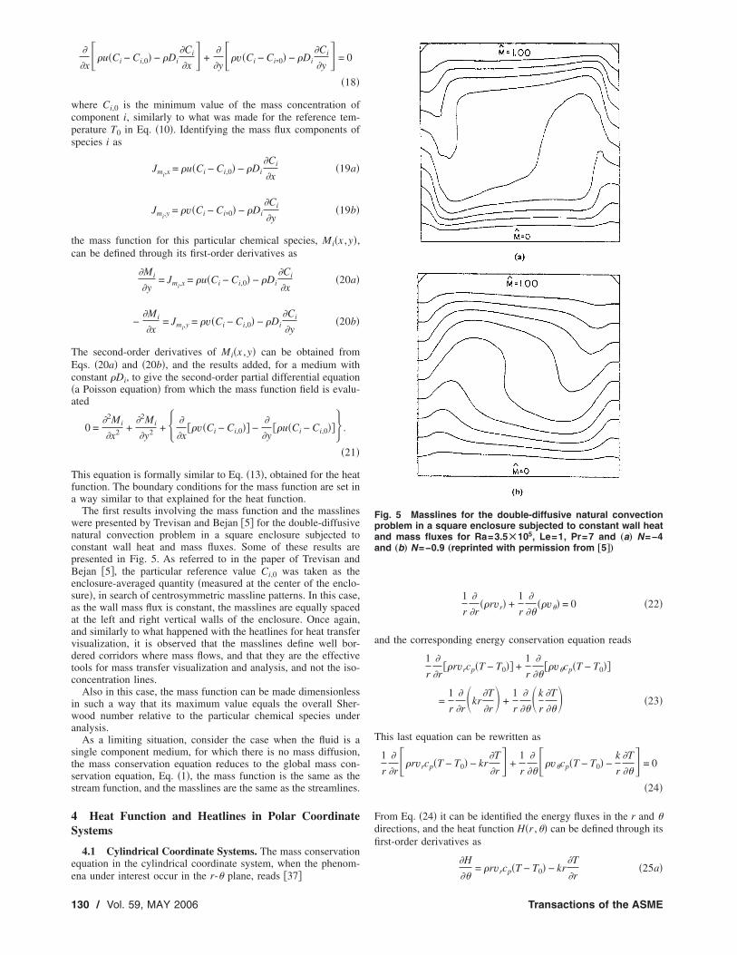
The first results involving the mass function and the masslineswere presented by Trevisan and Bejan �5� for the double-diffusivenatural convection problem in a square enclosure subjected toconstant wall heat and mass fluxes. Some of these results arepresented in Fig. 5. As referred to in the paper of Trevisan andBejan �5�, the particular reference value Ci,0 was taken as theenclosure-averaged quantity �measured at the center of the enclo-sure�, in search of centrosymmetric massline patterns. In this case,as the wall mass flux is constant, the masslines are equally spacedat the left and right vertical walls of the enclosure. Once again,and similarly to what happened with the heatlines for heat transfervisualization, it is observed that the masslines define well bor-dered corridors where mass flows, and that they are the effectivetools for mass transfer visualization and analysis, and not the iso-concentration lines.
Also in this case, the mass function can be made dimensionlessin such a way that its maximum value equals the overall Sher-wood number relative to the particular chemical species underanalysis.
As a limiting situation, consider the case when the fluid is asingle component medium, for which there is no mass diffusion,the mass conservation equation reduces to the global mass con-servation equation, Eq. �1�, the mass function is the same as thestream function, and the masslines are the same as the streamlines.
4 Heat Function and Heatlines in Polar CoordinateSystems
4.1 Cylindrical Coordinate Systems. The mass conservationequation in the cylindrical coordinate system, when the phenom-
ena under interest occur in the r-� plane, reads �37�130 / Vol. 59, MAY 2006
1
r
�
�r��rvr� +
1
r
�
����v�� = 0 �22�
and the corresponding energy conservation equation reads
1
r
�
�r��rvrcp�T − T0�� +
1
r
�
����v�cp�T − T0��
=1
r
�
�r�kr
�T
�r� +
1
r
�
��� k
r
�T
��� �23�
This last equation can be rewritten as
1
r
�
�r��rvrcp�T − T0� − kr
�T
�r� +
1
r
�
����v�cp�T − T0� −
k
r
�T
��� = 0
�24�
From Eq. �24� it can be identified the energy fluxes in the r and �directions, and the heat function H�r ,�� can be defined through itsfirst-order derivatives as
�H= �rvrcp�T − T0� − kr
�T�25a�
Fig. 5 Masslines for the double-diffusive natural convectionproblem in a square enclosure subjected to constant wall heatand mass fluxes for Ra=3.5Ã105, Le=1, Pr=7 and „a… N=−4and „b… N=−0.9 „reprinted with permission from †5‡…
�� �r
Transactions of the ASME
−�H
�r= �v�cp�T − T0� −
k
r
�T
���25b�
Evaluating the second-order crossed derivatives of H�r ,�� fromEqs. �25a� and �25b�, Eq. �24� is identically obtained.
If, instead, the plane of interest is the r-z plane, the mass con-servation equation reads �37�
1
r
�
�r��rvr� +
�
�z��vz� = 0 �26�
and the corresponding energy conservation equation reads
1
r
�
�r��rvrcp�T − T0�� +
�
�z��vzcp�T − T0��
=1
r
�
�r�kr
�T
�r� +
�
�z�k
�T
�z� �27�
which can be rewritten as
1
r
�
�r��rvrcp�T − T0� − kr
�T
�r� +
�
�z��vzcp�T − T0� − k
�T
�z� = 0
�28�
From this last equation it can be identified the energy fluxes in ther and z directions, and the heat function H�r ,z� can be defined
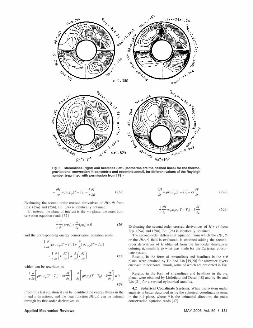
Fig. 6 Streamlines „right… and heatlines „left…gravitational convection in concentric and eccnumber „reprinted with permission from †19‡…
through its first-order derivatives as
Applied Mechanics Reviews
�H
�z= �rvrcp�T − T0� − kr
�T
�r�29a�
−1
r
�H
�r= �vzcp�T − T0� − k
�T
�z�29b�
Evaluating the second-order crossed derivatives of H�r ,z� fromEqs. �29a� and �29b�, Eq. �28� is identically obtained.
The second-order differential equation, from which the H�r ,��or the H�r ,z� field is evaluated, is obtained adding the second-order derivatives of H obtained from the first-order derivativesdefining it, similarly to what was made for the Cartesian coordi-nate system.
Results, in the form of streamlines and heatlines in the r-�plane, were obtained by Ho and Lin �19,20� for air/water layersenclosed in horizontal annuli, some of which are presented in Fig.6.
Results, in the form of streamlines and heatlines in the r-zplane, were obtained by Littlefield and Desai �18� and by Ho andLin �21� for a vertical cylindrical annulus.
4.2 Spherical Coordinate Systems. When the system underanalysis is better described using the spherical coordinate system,in the r-� plane, where � is the azimuthal direction, the mass
otherms are the dashed lines… for the thermo-tric annuli, for different values of the Rayleigh
„isen
conservation equation reads �37�
MAY 2006, Vol. 59 / 131
1
r2
�
�r��r2vr� +
1
r sin �
�
����v� sin �� = 0 �30�
and the energy conservation equation reads
1
r2
�
�r��r2vrcp�T − T0�� +
1
r sin �
�
����v� sin �cp�T − T0��
=1
r2
�
�r�r2k
�T
�r� +
1
r sin �
�
��� k
rsin �
�T
��� �31�
which can be rewritten as
1
r2
�
�r��r2vrcp�T − T0� − r2k
�T
�r� +
1
r sin �
�
����v� sin �cp�T − T0�
−k
rsin �
�T
��� = 0 �32�
From this last equation it can be identified the energy fluxes in ther and � directions, and the heat function H�r ,�� in the sphericalcoordinate system can be defined through its first-order deriva-tives as
1
sin �
�H
��= �r2vrcp�T − T0� − r2k
�T
�r�33a�
−1
r
�H
�r= �v� sin �cp�T − T0� −
k
rsin �
�T
���33b�
Evaluating the second-order crossed derivatives of H�r ,�� fromEqs. �33a� and �33b�, Eq. �32� is identically obtained.
The second-order differential equation, from which the H�r ,��field is evaluated, is obtained adding the second-order derivativesof H obtained from the first-order derivatives defining it, similarlyto what was made before for the Cartesian coordinate system.
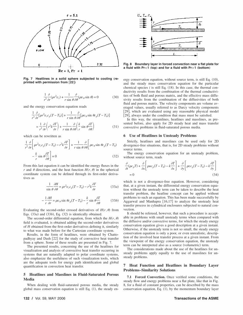
Results, in the form of heatlines, were obtained by Chatto-padhyay and Dash �22� for the study of convective heat transferfrom a sphere. Some of these results are presented in Fig. 7.
The presented results, concerning the use of the heatlines forvisualization and analysis of convective heat transfer occurring insystems that are naturally adapted to polar coordinate systems,also emphasize the usefulness of such visualization tools, whichare the adequate tools for energy path identification and globalquantification in convection heat transfer.
5 Heatlines and Masslines in Fluid-Saturated PorousMedia
When dealing with fluid-saturated porous media, the steady
Fig. 7 Heatlines in a solid sphere subjected to cooling „re-printed with permission from †22‡…
global mass conservation equation is still Eq. �1�, the steady en-
132 / Vol. 59, MAY 2006
ergy conservation equation, without source term, is still Eq. �10�,and the steady mass conservation equation for the particularchemical species i is still Eq. �18�. In this case, the thermal con-ductivity results from the combination of the thermal conductivi-ties of both fluid and porous matrix, and the effective mass diffu-sivity results from the combination of the diffusivities of bothfluid and porous matrix. The velocity components are volume av-eraged values, usually referred to as Darcy velocity components�29�, which are evaluated using any reasonable physical model�29�, always under the condition that mass must be satisfied.
In this way, the streamlines, heatlines and masslines, as pre-sented before, also apply for 2D steady heat and mass transferconvective problems in fluid-saturated porous media.
6 Use of Heatlines in Unsteady ProblemsStrictly, heatlines and masslines can be used only for 2D
divergence-free situations, that is, for 2D steady problems withoutsource terms.
The energy conservation equation for an unsteady problem,without source term, reads
�
�t��cpT� +
�
�x��ucp�T − T0� − k
�T
�x� +
�
�y��vcp�T − T0� − k
�T
�y�
= 0 �34�
which is not a divergence-free equation. However, consideringthat, at a given instant, the differential energy conservation equa-tion without the unsteady term can be taken to describe the heattransfer problem, the heatline concept can be applied withoutproblems to such an equation. This has been made successfully byAggarwal and Manhapra �16,17� to analyze the unsteady heattransfer process in cylindrical enclosures subjected to natural con-vection.
It should be refereed, however, that such a procedure is accept-able in problems with small unsteady terms when compared withthe diffusive and/or convective terms, for which the steady energyconservation equation gives a good description at a given instant.Otherwise, if the unsteady term is not so small, the steady energyconservation equation is only a poor, or even unrealistic, descrip-tion of the involved heat transfer process at a given instant. Fromthe viewpoint of the energy conservation equation, the unsteadyterm can be interpreted also as a source �volumetric� term.
The considerations made about the use of the heatlines for un-steady problems apply equally to the use of masslines for un-steady problems.
7 Heat Function and Heatlines in Boundary LayerProblems–Similarity Solutions
7.1 Forced Convection. Once verified some conditions, thesteady flow and energy problems near a flat plate, like that in Fig.8, for a fluid of constant properties, can be described by the mass
Fig. 8 Boundary layer in forced convection near a flat plate fora fluid with Pr<1 „top… and for a fluid with Pr>1 „bottom…
conservation equation, Eq. �1�, by the momentum boundary layer
Transactions of the ASME
equation, and by the boundary layer energy conservation equation.These equations read, respectively, as given by Bejan �27�
�u
�x+
�v�y
= 0 �35�
u�u
�x+ v
�u
�y= �
�2u
�y2 �36�
�cP�u�T
�x+ v
�T
�y� = k
�2T
�y2 �37�
A similarity solution can be obtained for the flow problem, andalso for the heat transfer problem. As the flow is forced, and it isnot influenced by the temperature field, the similarity solution forthe flow problem is obtained first. The developments that followare essentially due to Al Morega and Bejan �23�.
Making the Cartesian coordinates dimensionless as x*=x /L andy*= �y /L�ReL
1/2, where ReL=U�L /� as is the L-based Reynoldsnumber, it can be defined as the dimensionless similarity variableas
�x*,y*� = �y/x�Rex1/2 = y*x*
−1/2 �38�
where Rex=U�x /� is the x-based Reynolds number. The streamfunction is made dimensionless as �*=� / �U�L�, and it can beexpressed as
�*�x*,� = ReL−1/2 x*
1/2f�� �39�
where f�� is the dimensionless similarity function.The dimensionless velocity components �u* ,v*�= �u ,v� /U� are
obtained from the dimensionless stream function as
u* = ReL1/2���*/�y*� = f� �40a�
v* = − ��*/�x* = 12 ReL
−1/2 x*−1/2�f� − f� �40b�
where f�=df /d and it should be noted that the reference lengthsused to make the space coordinates dimensionless are related byReL
1/2. Thus, once the solution of the similarity function is known,the stream function is known and the velocity components are alsoknown.
Substitution of the dimensionless velocity components, as givenby Eqs. �40a� and �40b�, into the momentum boundary layer equa-tion, Eq. �36�, leads to
2f� + f f� = 0 �41�
an ordinary differential equation subjected to the boundary condi-tions f�0�= f��0�=0 and f��+��=1. Equation �41� depends onlyon the variable, and the main advantage of the similarity trans-formation is the reduction of the number of independent variablesfrom two, x ,y, to one, . The solution of the boundary layer flowproblem is evaluated from the solution of Eq. �41�.
Once the flow solution is known, the heat transfer problem canalso be solved using the similarity transformation. Substitution ofthe velocity components as given by Eqs. �40a� and �40b� into theboundary layer energy conservation equation, Eq. �37�, makingthe temperature dimensionless as ��x ,y�= �T�x ,y�−Tw� / �T�−Tw�,one obtains
�� + �Pr/2�f�� = 0 �42�
where it can be made T�x ,y�=T��, and �=��� only. The heattransfer problem is solved once the solution of Eq. �42� is known,subjected to the boundary conditions ��0�=0 and ��+��=1.
The heat function for this problem is defined using the expres-sions given by Eqs. �12a� and �12b�, noting that, in this case, thediffusive term in Eq. �12a� does not exist. The heat function ismade dimensionless using the convective term and not the diffu-
sive term as made before, through the expressionApplied Mechanics Reviews
H* =H
�cPU� T� − Tw L ReL−1/2 �43�
where T�−Tw =T�−Tw for an isothermal cold wall and T�
−Tw =Tw−T� for an isothermal hot wall.It should be noted that the global heat transfer between the wall
of length L and the stream can be obtained, in a scale sense, froman energy balance made to the thermal boundary layer. Such en-
ergy balace gives Q� mcP�T�−Tw�=�ucP�T�−Tw�T, where T isthe thickness of the thermal boundary layer and u is the velocity atthe leading edge of the thermal boundary layer. For a fluid with
Pr�1 it is T�L Pr−1/2 ReL−1/2 and u�U�, and it is Q
��U�cP�T�−Tw�L ReL−1/2 Pr−1/2. For a fluid with Pr�1 it is T
�L Pr−1/3 ReL−1/2 and u�U��T /�, and it is Q��U�cP�T�
−Tw�L ReL−1/2 Pr−2/3. In this way, as Q�hL�T�−Tw� and Nu
=hL /k, it is Nu� Q / �k�T�−Tw��. The overall Nusselt number isproportional to Re1/2 Pr1/2 for a fluid with Pr�1, and the overallNusselt number is proportional to Re1/2 Pr1/3 for a fluid with Pr�1. These proportionalities have been explored in depth by AlMorega and Bejan �23�.
The dimensionless first-order derivatives that define the heat-function near an isothermal cold wall become
�H*
�y*= f�� �44a�
−�H*
�x*=
1
2x*
−1/2�f� − f�� −1
Pr
��
�y*�44b�
and it is assumed that H*�x* ,y*� is given by an expression of theform
H*�x*,y*� = x*1/2g��x*,y*�� �45�
Function g is found to be
g�� = f� +2
Pr�� �46�
which gives, for the similarity solution for the heat function
H*�x*,� = x*1/2� f� +
2
Pr��� �47�
under the assumption that H*�0,0�=0.Similarly it can be obtained the similarity solution for the heat
function near an isothermal hot wall as
H*�x*,� = − x*1/2� f�� − 1� +
2
Pr��� �48�
also under the assumption that H*�0,0�=0.At the wall it is =0 and f�0�=0, and �� is a function of the
Prandtl number only, as given by Bejan �27�, and the heat functionincreases with x*
1/2 along the cold wall and decreases with −x*1/2
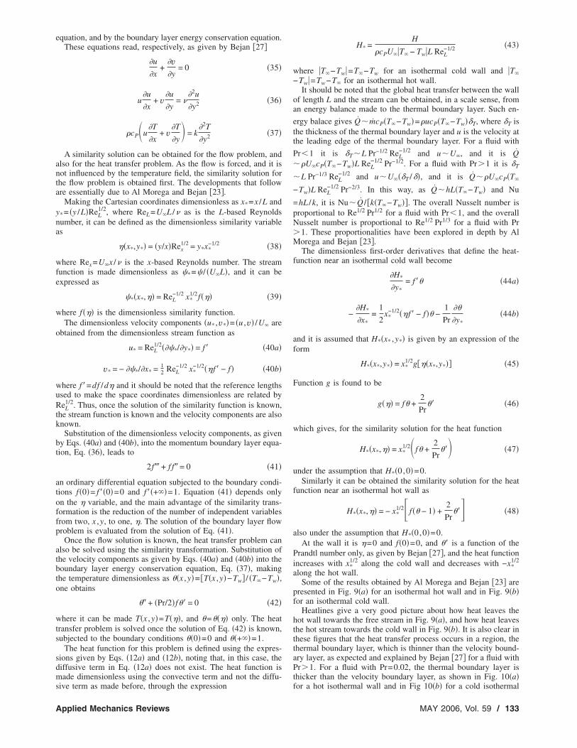
along the hot wall.Some of the results obtained by Al Morega and Bejan �23� are
presented in Fig. 9�a� for an isothermal hot wall and in Fig. 9�b�for an isothermal cold wall.
Heatlines give a very good picture about how heat leaves thehot wall towards the free stream in Fig. 9�a�, and how heat leavesthe hot stream towards the cold wall in Fig. 9�b�. It is also clear inthese figures that the heat transfer process occurs in a region, thethermal boundary layer, which is thinner than the velocity bound-ary layer, as expected and explained by Bejan �27� for a fluid withPr�1. For a fluid with Pr=0.02, the thermal boundary layer isthicker than the velocity boundary layer, as shown in Fig. 10�a�
for a hot isothermal wall and in Fig 10�b� for a cold isothermalMAY 2006, Vol. 59 / 133
wall.The similarity solution for the heat function can also be ob-
tained for the situation of a hot wall with uniform heat flux. In thiscase, the temperature in the boundary layer changes as
T�x,y� = T� +q�
k� �x
U��1/2
��� �49�
and the similarity version of the heat transfer problem is given bythe equation
�� +Pr
2�f�� − f��� = 0 �50�
satisfying the boundary conditions ���0�=−1 and ��+��=0.In this case, the heat function is made dimensionless as
H*�x*,y*� =H�x,y�
q�L�51�
noting that q�L is the global heat transfer exchange between thewall and the fluid, and the first-order derivatives that define theheat function are
�H* = Pr x*1/2f�� �52a�
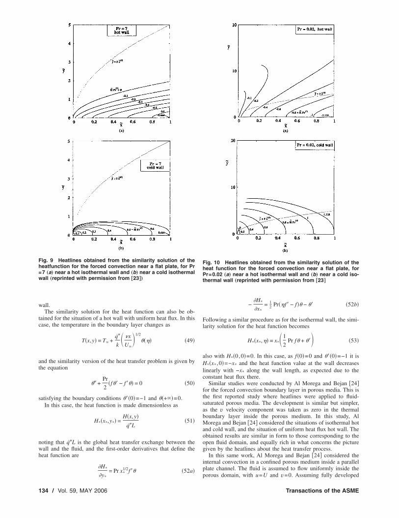
Fig. 9 Heatlines obtained from the similarity solution of theheatfunction for the forced convection near a flat plate, for Pr=7 „a… near a hot isothermal wall and „b… near a cold isothermalwall „reprinted with permission from †23‡…
�y*
134 / Vol. 59, MAY 2006
−�H*
�x*= 1
2 Pr�f� − f�� − �� �52b�
Following a similar procedure as for the isothermal wall, the simi-larity solution for the heat function becomes
H*�x*,� = x*�1
2Pr f� + ��� �53�
also with H*�0,0�=0. In this case, as f�0�=0 and ���0�=−1 it isH*�x* ,0�=−x* and the heat function value at the wall decreaseslinearly with −x* along the wall length, as expected due to theconstant heat flux there.
Similar studies were conducted by Al Morega and Bejan �24�for the forced convection boundary layer in porous media. This isthe first reported study where heatlines were applied to fluid-saturated porous media. The development is similar but simpler,as the v velocity component was taken as zero in the thermalboundary layer inside the porous medium. In this study, AlMorega and Bejan �24� considered the situations of isothermal hotand cold wall, and the situation of uniform heat flux hot wall. Theobtained results are similar in form to those corresponding to theopen fluid domain, and equally rich in what concerns the picturegiven by the heatlines about the heat transfer process.
In this same work, Al Morega and Bejan �24� considered theinternal convection in a confined porous medium inside a parallelplate channel. The fluid is assumed to flow uniformly inside the
Fig. 10 Heatlines obtained from the similarity solution of theheat function for the forced convection near a flat plate, forPr=0.02 „a… near a hot isothermal wall and „b… near a cold iso-thermal wall „reprinted with permission from †23‡
porous domain, with u=U and v=0. Assuming fully developed
Transactions of the ASME
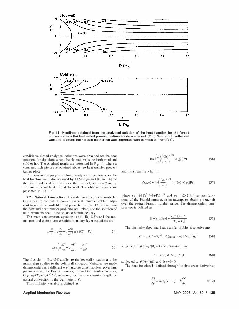
conditions, closed analytical solutions were obtained for the heatfunction, for situations where the channel walls are isothermal andcold or hot. The obtained results are presented in Fig. 11, where aclear and rich picture is obtained about the heat transfer processtaking place.
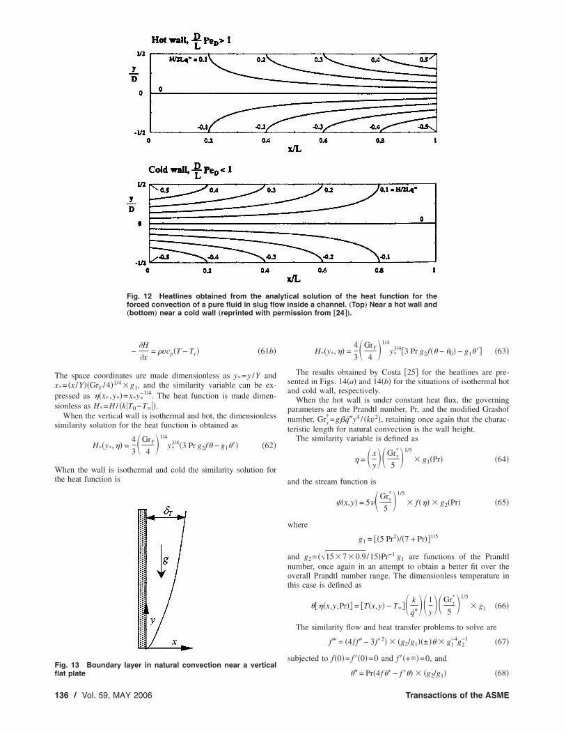
For comparison purposes, closed analytical expressions for theheat function were also obtained by Al Morega and Bejan �24� forthe pure fluid in slug flow inside the channel, with u=U and v=0, and constant heat flux at the wall. The obtained results arepresented in Fig. 12.
7.2 Natural Convection. A similar treatment was made byCosta �25� to the natural convection heat transfer problem adja-cent to a vertical wall like that presented in Fig. 13. In this casethe flow and heat transfer problems are linked, and the solution ofboth problems need to be obtained simultaneously.
The mass conservation equation is still Eq. �35�, and the mo-mentum and energy conservation boundary layer equations are
u�v�x
+ v�v�y
= ��2v�x2 ± g��T − T�� �54�
�cP�u�T
�x+ v
�T
�y� = k
�2T
�x2 �55�
The plus sign in Eq. �54� applies to the hot wall situation and theminus sign applies to the cold wall situation. Variables are madedimensionless in a different way, and the dimensionless governingparameters are the Prandtl number, Pr, and the Grashof number,GrY =g��TH−TC�Y3 /�2, retaining that the characteristic length fornatural convection is the wall height, Y.
Fig. 11 Heatlines obtained from the analyticconvection in a fluid-saturated porous mediuwall and „bottom… near a cold isothermal wall
The similarity variable is defined as
Applied Mechanics Reviews
= � x
y��Gry
4�1/4
� g1�Pr� �56�
and the stream function is
��x,y� = 4��Gry
4�1/4
� f�� � g2�Pr� �57�
where g1= ��4 Pr2� / �4+Pr��1/4 and g2= �2/2�Pr−1 g1 are func-tions of the Prandtl number, in an attempt to obtain a better fitover the overall Prandtl number range. The dimensionless tem-perature is defined as
���x,y,Pr�� =T�x,y� − T�
Tw − T� �58�
The similarity flow and heat transfer problems to solve are
f� = �3f f� − 2f�2� � �g2/g1��±�� � g1−3g2
−1 �59�
subjected to f�0�= f��0�=0 and f��+��=0, and
�� = 3 Pr f�� � �g2/g1� �60�
subjected to ��0�= �±�1 and ��+��=0.The heat function is defined through its first-order derivatives
as
�H= �ucp�T − Tc� − k
�T�61a�
solution of the heat function for the forcednside a channel. „Top… Near a hot isothermalprinted with permission from †24‡….
alm i„re
�y �x
MAY 2006, Vol. 59 / 135
erm
−�H
�x= �vcp�T − Tc� �61b�
The space coordinates are made dimensionless as y*=y /Y andx*= �x /Y��GrY /4�1/4�g1, and the similarity variable can be ex-pressed as �x* ,y*�=x*y*
−1/4. The heat function is made dimen-sionless as H*=H / �k T0−T� �.
When the vertical wall is isothermal and hot, the dimensionlesssimilarity solution for the heat function is obtained as
H*�y*,� =4
3�GrY
4�1/4
y*3/4�3 Pr g2f� − g1��� �62�
When the wall is isothermal and cold the similarity solution forthe heat function is
Fig. 12 Heatlines obtained from the anaforced convection of a pure fluid in slug flo„bottom… near a cold wall „reprinted with p
Fig. 13 Boundary layer in natural convection near a vertical
flat plate136 / Vol. 59, MAY 2006
H*�y*,� =4
3�GrY
4�1/4
y*3/4�3 Pr g2f�� − �0� − g1��� �63�
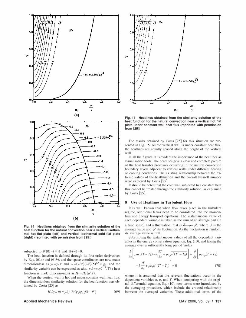
The results obtained by Costa �25� for the heatlines are pre-sented in Figs. 14�a� and 14�b� for the situations of isothermal hotand cold wall, respectively.
When the hot wall is under constant heat flux, the governingparameters are the Prandtl number, Pr, and the modified Grashofnumber, Gry
*=g�q�y4 / �kv2�, retaining once again that the charac-teristic length for natural convection is the wall height.
The similarity variable is defined as
= � x
y��Gry
*
5�1/5
� g1�Pr� �64�
and the stream function is
��x,y� = 5��Gry*
5�1/5
� f�� � g2�Pr� �65�
where
g1 = ��5 Pr2�/�7 + Pr��1/5
and g2= �15�7�0.9/15�Pr−1 g1 are functions of the Prandtlnumber, once again in an attempt to obtain a better fit over theoverall Prandtl number range. The dimensionless temperature inthis case is defined as
���x,y,Pr�� = �T�x,y� − T��� k
q���1
y��Gry
*
5�1/5
� g1 �66�
The similarity flow and heat transfer problems to solve are
f� = �4f f� − 3f�2� � �g2/g1��±�� � g1−4g2
−1 �67�
subjected to f�0�= f��0�=0 and f��+��=0, and
cal solution of the heat function for thenside a channel. „Top… Near a hot wall andission from †24‡….
lytiw i
�� = Pr�4f�� − f��� � �g2/g1� �68�
Transactions of the ASME
subjected to ���0�= � �1 and ��+��=0.The heat function is defined through its first-order derivatives
by Eqs. �61a� and �61b�, and the space coordinates are now madedimensionless as y*=y /Y and x*= �x /Y��GrY
* /5�1/5�g1, and thesimilarity variable can be expressed as �x* ,y*�=x*y*
−1/5. The heatfunction is made dimensionless as H*=H / �q�Y�.
When the vertical wall is hot and under constant wall heat flux,the dimensionless similarity solution for the heatfunction was ob-tained by Costa �25� as
Fig. 14 Heatlines obtained from the similarity solution of theheat function for the natural convection near a vertical isother-mal hot flat plate „left… and vertical isothermal cold flat plate„right… „reprinted with permission from †25‡…
H*�y*,� = y*�4 Pr�g2/g1�f� − ��� �69�
Applied Mechanics Reviews
The results obtained by Costa �25� for this situation are pre-sented in Fig. 15. As the vertical wall is under constant heat flux,the heatlines are equally spaced along the height of the verticalwall.
In all the figures, it is evident the importance of the heatlines asvisualization tools. The heatlines give a clear and complete pictureof the heat transfer processes occurring in the natural convectionboundary layers adjacent to vertical walls under different heatingor cooling conditions. The existing relationship between the ex-treme values of the heatfunction and the overall Nusselt numberwere explored by Costa �25�.
It should be noted that the cold wall subjected to a constant heatflux cannot be treated through the similarity solution, as explainedby Costa �25�.
8 Use of Heatlines in Turbulent FlowIt is well known that when flow takes place in the turbulent
regime, additional terms need to be considered into the momen-tum and energy transport equations. The instantaneous value ofeach dependent variable is taken as the sum of an average part �ina time sense� and a fluctuation, that is �=�+��, where � is theaverage value and �� its fluctuation. As the fluctuation is random,its average value is null.
Substituting the instantaneous values of all the dependent vari-ables in the energy conservation equation, Eq. �10�, and taking theaverage over a sufficiently long period yields
�
�x��ucp�T − T0� − k
�T
�x+ �cpu��T� − T0�� +
�
�y��vcp�T − T0�
− k�T
�y+ �cpv��T� − T0�� = 0 �70�
where it is assumed that the relevant fluctuations occur in thedependent variables u, v, and T. When comparing with the origi-nal differential equation, Eq. �10�, new terms were introduced bythe averaging procedure, which include the crossed relationship
Fig. 15 Heatlines obtained from the similarity solution of theheat function for the natural convection near a vertical hot flatplate under constant wall heat flux „reprinted with permissionfrom †25‡…
between the averaged variables. These additional terms, of the
MAY 2006, Vol. 59 / 137

form Fi=−�cpui��T�−T0�, are known as the turbulent fluxes, andthey are evaluated using a turbulence model �27�.
Once these additional terms are evaluated using an availableprocedure, the heatfunction in turbulent convective heat transfercan be defined through its first-order derivatives, using Eq. �70�,as
�H
�y= �ucp�T − T0� − k
�T
�x+ �cpu��T� − T0� �71a�
−�H
�x= �vcp�T − T0� − k
�T
�y+ �cpv��T� − T0� �71b�
The differential equation for the heatfunction field is evaluated inthe same way as for the laminar case, but now using Eqs. �71a�and �71b�, and it results in
0 =�2H
�x2 +�2H
�y2 +�
�x��vcp�T − T0� + �cpv��T� − T0��
−�
�y��ucp�T − T0� + �cpu��T� − T0�� �72�
From this point forward, the turbulent situation is treated in thesame way as the laminar situation.
Dash �26� used that formulation to obtain the heatlines corre-sponding to the turbulent heat transfer near a heated vertical plate.
If the heat transfer problem under analysis occurs in the turbu-lent boundary layer near a wall, the heatline concept can be ap-plied in a simpler way, by using an effective diffusion coefficientfor heat. In this case, the heat function is defined through itsfirst-order derivatives as usually for the boundary layer adjacent toa flat plate �27�
�H
�y= �ucp�T − T0� �73a�
−�H
�x= �vcp�T − T0� − �k + �cp�H�
�T
�y�73b�
where the turbulent flux has been expressed as −�cpv��T�−T0�=�cp�H��T /�y�. Some results involving the heatlines were ob-tained by Bejan �27�, using such an approach for turbulent bound-ary layers near hot and cold isothermal walls.
9 Unification of the Streamline, Heatline, andMassline Methods
The streamline, heatline, and massline methods were unified byCosta �30�, in order to be subjected to a common treatment, and inorder to be easily included, through a common procedure, intoCFD packages.
The differential conservation equation for the general variable
Table 1 The physical meaning of �, and
Physical principle � ��
Overall mass conservation 1 0Energy conservation T k /cP
i species mass conservation Ci �Di
F, whose specific value is �=F /m, can be written as
138 / Vol. 59, MAY 2006
�
�x��u�� − �0� − ��
��
�x� +
�
�y��v�� − �0� − ��
��
�y� = 0
�74�
where �0 is a reference value for �, taken as its lower value in theentire domain under analysis. In Eq. �74� are identified the fluxcomponents of the total flux J� as
J�,x = �u�� − �0� − ��
��
�x�75a�
J�,y = �v�� − �0� − ��
��
�y�75b�
Function ��x ,y�, associated with the variable �, and whose con-tour plots will be used for visualization and analysis purposes, isdefined through its first order derivatives as
��
�y= �u�� − �0� − ��
��
�x�76a�
−��
�x= �v�� − �0� − ��
��
�y�76b�
Equation �74� can be identically obtained by equating the secondorder crossed derivatives of � evaluated from Eqs. �76a� and�76b�, being implicitly assumed that ��x ,y� is a continuous func-tion to its second order derivatives.
Assuming now that � is a continuous function to its secondorder derivatives, one can establish the equality of its second or-der crossed derivatives through the expressions obtained from theright-hand sides of Eqs. �76a� and �76b�, leading to
0 =�
�x� 1
��
��
�x� +
�
�y� 1
��
��
�y� + �
�x� �v
��
�� − �0��−
�
�y� �u
��
�� − �0��� �77�
This is the second-order partial differential equation �a Poissonequation� from which it is evaluated in the � field, for any par-ticular corresponding meaning of �. It is an equation correspond-ing to a conduction-type problem, with source term if the fluidflow subsists, and without source term if the fluid flow subsides,with the diffusion coefficient for � verifying
�� = 1/�� �78�
The diffusion coefficient ��=1/�� is maintained within parenthe-ses in Eq. �77� because it is, in the general case, a variable and nota constant. To the author’s knowledge, this was the first formula-tion considering a variable diffusion coefficient for �.
For �=1, �0=0, and ��=�, a small constant number, one ob-tains the well-known partial differential equation for the streamfunction, Eq. �5�. The particular meaning of � and its respective�, whose contour plots are used for visualization and analysispurposes, for some usual situations, are summarized in Table 1.
In what concerns the boundary conditions for Eq. �77�, they can
pling with �, for frequent situations †30‡.
� � contour plots
�, stream function StreamlinesH, heat function Heatlines
i, i species mass function i species masslines
cou
M
be specified as
Transactions of the ASME
��xref,y� = ��xref,yref� +�yref
y ��u�� − �0� − ��
��
�x�dy �79�
along a boundary with constant x, or as
��x,yref� = ��xref,yref� −�xref
x ��v�� − �0� − ��
��
�y�dx �80�
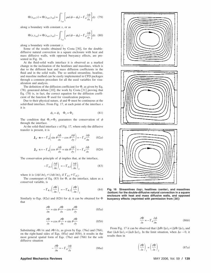
along a boundary with constant y.Some of the results obtained by Costa �30�, for the double-
diffusive natural convection in a square enclosure with heat andmass diffusive walls, with opposed buoyancy effects, are pre-sented in Fig. 16.
At the fluid-solid walls interface it is observed as a markedchange in the inclination of the heatlines and masslines, which isdue to the different heat and mass diffusion coefficients in thefluid and in the solid walls. The so unified streamline, heatline,and massline method can be easily implemented in CFD packagesthrough a common procedure for all the used variables for visu-alization and analysis.
The definition of the diffusion coefficient for �, as given by Eq.�78�, generated debate �10�; the work by Costa �31� proving thatEq. �78� is, in fact, the correct equation for the diffusion coeffi-cient of the function � used for visualization purposes.
Due to their physical nature, � and � must be continuous at thesolid-fluid interface. From Fig. 17, at each point of the interface sit is
�1 = �2 �1 = �2 �81�
The condition that �1=�2 guarantees the conservation of �through the interface.
At the solid-fluid interface s of Fig. 17, where only the diffusivetransfer is present, it is
J� · n = − ���sin ���
�x− cos �
��
�y� = − ��
��
�n�82a�
J� · s = − ���cos ���
�x+ sin �
��
�y� = − ��
��
�s�82b�
The conservation principle of � implies that, at the interface,
− ��,1� ��
�n�
1= − ��,2� ��
�n�
2�83�
where it is ��� /�n�1� ��� /�n�2 if ��,1���,2.The counterpart of Eq. �83� for �, at the interface, taken as a
conserved variable, is
− ��,1� ��
�n�
1= − ��,2� ��
�n�
2�84�
Similarly to Eqs. �82a� and �82b� for �, it can be obtained for �that
��
�n= sin �
��
�x− cos �
��
�y�85a�
��
�s= cos �
��
�x+ sin �
��
�y�85b�
Substituting �� /�x and �� /�y, as given by Eqs. �76a� and �76b�,on the right-hand sides of Eqs. �85a� and �85b�, it results in themost general spatial form of Eqs. �76a� and �76b� for the solediffusive situation
−��
= − ��
���86a�
�n �s
Applied Mechanics Reviews
��
�s= − ��
��
�n�86b�
From Fig. 17 it can be observed that ��� /�s�1= ��� /�s�2 andthat ��� /�s�1= ��� /�s�2. In the limit situation, when �s→0, itresults then in
� ��
�s� = � ��
�s� �87a�
Fig. 16 Streamlines „top…, heatlines „center…, and masslines„bottom… for the double-diffusive natural convection in a squareenclosure with heat and mass diffusive walls, and opposedbuoyancy effects „reprinted with permission from †30‡…
1 2
MAY 2006, Vol. 59 / 139

� ��
�s�
1= � ��
�s�
2�87b�
Joining together Eqs. �87b� and �86a�, it can be stated that
−1
��,1� ��
�n�
1= −
1
��,2� ��
�n�
2�88�
Comparing this result with Eq. �84� it is evident that, in fact, it is��=1/��.
The change in direction of the contour plots used for visualiza-tion and analysis, due to the existence of adjacent media withdifferent diffusion coefficients, can be referred to as the refractionof the heatlines and/or masslines. In fact, a similar situation occurswith the streamlines when analyzing fluid flow in adjacent mediaof different permeabilities, what is referred to as the refraction ofthe streamlines in the groundwater bibliography �38,39�.
10 Unification of the Streamline, Heatline andMassline Methods for Anisotropic Media
The streamline, heatline, and massline methods have been uni-fied by Costa �32� to apply to anisotropic media, which are ofgreat and increasing practical interest. Recognizing that, in thiscase, the flux transport components are
J�,x = �u�� − �0� − ����,�l12 + ��,l2
2���
�x
+ ���,�l1m1 + ��,l2m2���
�y� �89a�
Fig. 17 Lines of constant � and lines of constant �, normal toeach other at any point, near the interface s between media 1and 2 of different diffusion coefficients „reprinted with permis-sion from †31‡…
Table 2 Physical principles, diffusion coefficmeanings of � †32‡
Physical Principle � ��,xx
Overall mass conservation 1 0i species mass conservation Ci �Di,xx
Energy conservation T kxx /cP
Overall mass conservation�Darcy flow model� p �Kxx /�
140 / Vol. 59, MAY 2006
J�,y = �v�� − �0� − ����,�l1m1 + ��,l2m2���
�x
+ ���,�m12 + ��,m2
2���
�y� �89b�
where u and v are the area averaged Cartesian velocity compo-nents �29�, ��,� and ��, are the principal diffusion coefficientsfor � along the � , principal Cartesian directions, which are re-lated with the x ,y Cartesian coordinate system through the direc-tion cosines l1 , l2 and m1 ,m2. With ��,xx=��,�l1
2+��,l22, ��,yy
=��,�m12+��,m2
2, and ��,xy =��,yx=��,�l1m1+��,l2m2, Eqs.�89a� and �89b� become
J�,x = �u�� − �0� − ���,xx��
�x+ ��,xy
��
�y� �90a�
J�,y = �v�� − �0� − ���,xy��
�x+ ��,yy
��
�y� �90b�
Inserting these fluxes into the general conservation equation, it isobtained the general convection-diffusion differential transportequation for � in two-dimensional anisotropic media
�
�x��u� − ���,xx
��
�x+ ��,xy
��
�y�� +
�
�y��v� − ���,xy
��
�x
+ ��,yy��
�y�� = 0 �91�
When dealing with fluid-saturated anisotropic porous media,the velocity components are usually related to the pressure gradi-ent and the body force �in this case only the gravitational accel-eration, being the x ,y coordinate system placed such that gx=0and gy =−g� through the Darcy flow model, which is sufficientlyaccurate for many practical applications �29�
u = −1
��Kxx
�p
�x+ Kxy� �p
�y+ �g�� �92a�
v = −1
��Kxy
�p
�x+ Kyy� �p
�y+ �g�� �92b�
However, if there are interfaces between fluid saturated porousmedia and pure fluids �the latter governed by the Navier-Stokesequations�, or the Reynolds number is high enough such that in-ertial effects must be taken into account, more detailed and com-plete models �usually the Brinkman and Forchheimer modifica-tions, respectively� are needed �29�.
Different physical meanings of � and its associated transportcoefficients can be found in Table 2.
The function ��x ,y�, whose contour plots are used for visual-ization purposes, is defined from Eqs. �90a� and �90b� through itsfirst order derivatives as
ts, and source terms for different particular
�,yy ��,xy S�
0 0 0Di,yy �Di,xy
0
yy /cP kxy /cP0
yy /� �Kxy /��
�x��2gKxy
�� +
�
�y��2gKyy
��
ien
�
�k
�K
Transactions of the ASME
��
�y= J�,x = �u�� − �0� − ���,xx
��
�x+ ��,xy
��
�y� �93a�
−��
�x= J�,y = �v�� − �0� − ���,xy
��
�x+ ��,yy
��
�y� �93b�
Equating the second-order mixed derivatives of �, being implic-itly assumed that it is a continuous function to its second orderderivatives, Eq. �91� is identically obtained.
From Eqs. �93a� and �93b� it can be obtained that
��
�x= −
��,yy
�2
��
�y−
��,xy
�2
��
�x+
��,yy
�2 �u�� − �0� −��,xy
�2 �v�� − �0�
�94a�
��
�y=
��,xx
�2
��
�x−
��,xy
�2
��
�y+
��,xx
�2 �v�� − �0� −��,xy
�2 �u�� − �0�
�94b�
where
�2 = ��,xx��,yy − ��,xy2 ��0� �95�
Assuming now that � is a continuous function to its secondorder derivatives, it can be established that the equality of itssecond order crossed derivatives, obtained from Eqs. �94a� and�94b�, lead to the equation
0 =�
�x���,xx
�2
��
�x� +
�
�y���,yy
�2
��
�y� + � �
�x���,xy
�2
��
�y�
+�
�y���,xy
�2
��
�x�� +
�
�x���� − �0�
�2 ���,xxv − ��,xyu��−
�
�y���� − �0�
�2 ���,yyu − ��,xyv�� �96�
This is the diffusion equation for � in anisotropic media, with thesource term present in the second and third rows. It is evidentfrom Eq. �96� that the diffusion coefficients for � in anisotropicmedia are
��,xx =��,xx
�2 ��,yy =��,yy
�2 ��,xy =��,xy
�2 �97�
If the x ,y coordinate system is coincident with the principal sys-tem, it is ��,xx=��,�=1/��, and ��,yy =��,=1/��,�, i.e., theprincipal diffusion coefficients for � are the inverse of the diffu-sion coefficient for � in the perpendicular directions. For isotropic
Table 3 Coupling of � and � and the diffusion
Physical principle � �
Overall mass conservation 1 � stream function
i species mass conservation Ci Mi, i species mass funct
Energy conservation T H, heat function
K2=KxxKyy −Kxy2 , Di
2=Di,xxDi,yy −Di,xy2 , and k2=kxxkyy −kxy
2
media, it comes that ��=1/��, as given by Eq. �78�.
Applied Mechanics Reviews
Similarly to what was made to obtain the differential equationfor �, defining the stream function � �overall mass function�through its first order derivatives as given by Eqs. �2a� and �2b� itis obtained the diffusion equation for � in anisotropic media,
0 =�
�x��Kxx
�K2
��
�x� +
�
�y��Kyy
�K2
��
�y� + � �
�x��Kxy
�K2
��
�y�
+�
�y��Kxy
�K2
��
�x�� −
�
�x��g� �98�
where K2=KxxKyy −Kxy2 , which is formally similar to Eq. �96�. It is
evident that the diffusion coefficients for � are
��,xx =�Kxx
�K2 ��,yy =�Kyy
�K2 ��,xy =�Kxy
�K2 �99�
The most common meaning of � and its associated � functionused for visualization and analysis purposes is summarized inTable 3.
In what concerns the boundary conditions for variable �, theycan be stated as
�P,B = �ref,B +�ref,B
P,B
J� · ndsB �100�
Due to their physical nature, � and � are C0 continua. Thus, ateach point of any interface between contiguous portions 1 and 2of the domain, even with different properties �as it is the case ofconjugate heat and/or mass transfer problems�, it is
�1 = �2 �101a�
�1 = �2 �101b�
Also due to its physical nature, �1=�2 �or �1=�2� guarantees theconservation of � through such an interface.
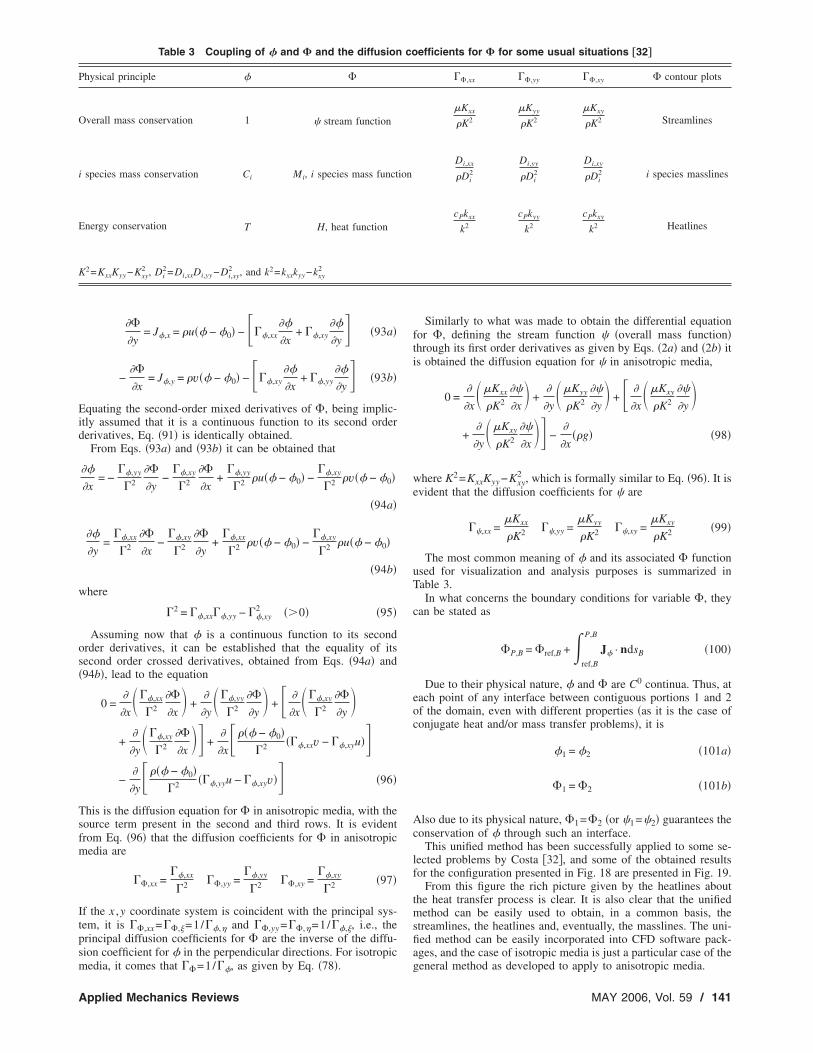
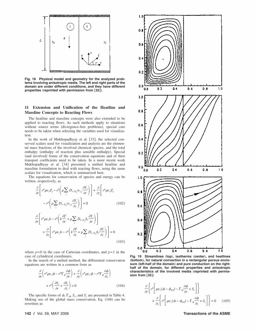
This unified method has been successfully applied to some se-lected problems by Costa �32�, and some of the obtained resultsfor the configuration presented in Fig. 18 are presented in Fig. 19.
From this figure the rich picture given by the heatlines aboutthe heat transfer process is clear. It is also clear that the unifiedmethod can be easily used to obtain, in a common basis, thestreamlines, the heatlines and, eventually, the masslines. The uni-fied method can be easily incorporated into CFD software pack-ages, and the case of isotropic media is just a particular case of the
efficients for � for some usual situations †32‡
��,xx ��,yy ��,xy � contour plots
�Kxx
�K2
�Kyy
�K2
�Kxy
�K2 Streamlines
Di,xx
�Di2
Di,yy
�Di2
Di,xy
�Di2 i species masslines
cPkxx
k2
cPkyy
k2
cPkxy
k2 Heatlines
co
ion
general method as developed to apply to anisotropic media.
MAY 2006, Vol. 59 / 141
11 Extension and Unification of the Heatline andMassline Concepts to Reacting Flows
The heatline and massline concepts were also extended to beapplied to reacting flows. As such methods apply to situationswithout source terms �divergence-free problems�, special careneeds to be taken when selecting the variables used for visualiza-tion.
In the work of Mukhopadhyay et al. �33�, the selected con-served scalars used for visualization and analysis are the elemen-tal mass fractions of the involved chemical species, and the totalenthalpy �enthalpy of reaction plus sensible enthalpy�. Special�and involved� forms of the conservation equations and of theirtransport coefficients need to be taken. In a more recent workMukhopadhyay et al. �34� presented a unified heatline andmassline formulation to deal with reacting flows, using the samescalars for visualization, which is summarized here.
The equations for conservation of species and energy can bewritten, respectively, as
�
�r�rp�vrZj − rp���i
Di−N2wi,j
�Yi
�r �� +�
�z�rp�vzZj
− rp���i
Di−N2wi,j
�Yi
�z �� = 0 �102�
�
�r�rp�vrh − rp�k�T
�r+ ��
i
Di−N2hi
�Yi
�r ��+
�
�z�rp�vzh − rp�k�T
�z+ ��
i
Di−N2hi
�Yi
�z �� = 0
�103�
where p=0 in the case of Cartesian coordinates, and p=1 in thecase of cylindrical coordinates.
In the search of a unified method, the differential conservationequations are written in a common form as
�
�r�rp�vr� − rp��
��
�r� +
�
�z�rp�vz� − rp��
��
�z�
+ rp� �Sr
�r+
�Sz
�z� = 0 �104�
The specific forms of �, ��, Sr, and Sz are presented in Table 4.Making use of the global mass conservation, Eq. �104� can be
Fig. 18 Physical model and geometry for the analyzed prob-lems involving anisotropic media. The left and right parts of thedomain are under different conditions, and they have differentproperties „reprinted with permission from †32‡….
rewritten as
142 / Vol. 59, MAY 2006
�
�rrp��vr�� − �ref� − ��
��
�r+ Sr��
+� rp��vz�� − �ref� − ��
��+ Sz�� = 0 �105�
Fig. 19 Streamlines „top…, isotherms „center…, and heatlines„bottom…, for natural convection in a rectangular porous enclo-sure „left-half of the domain… and pure conduction on the right-half of the domain, for different properties and anisotropiccharacteristics of the involved media „reprinted with permis-sion from †32‡…
�z �z
Transactions of the ASME
From that equation it can be identified the flux components ofthe conserved variable �. Its counterpart, �, used for visualizationand analysis purposes can then be defined through its first-orderderivatives as
��
�z= rp��vr�� − �ref� − ��
��
�r+ Sr� �106a�
−��
�r= rp��vz�� − �ref� − ��
��
�z+ Sz� �106b�
Equation �105� can be identically obtained by equating the secondorder crossed derivatives of �, assuming that it is a function con-tinuous to its second order derivatives.
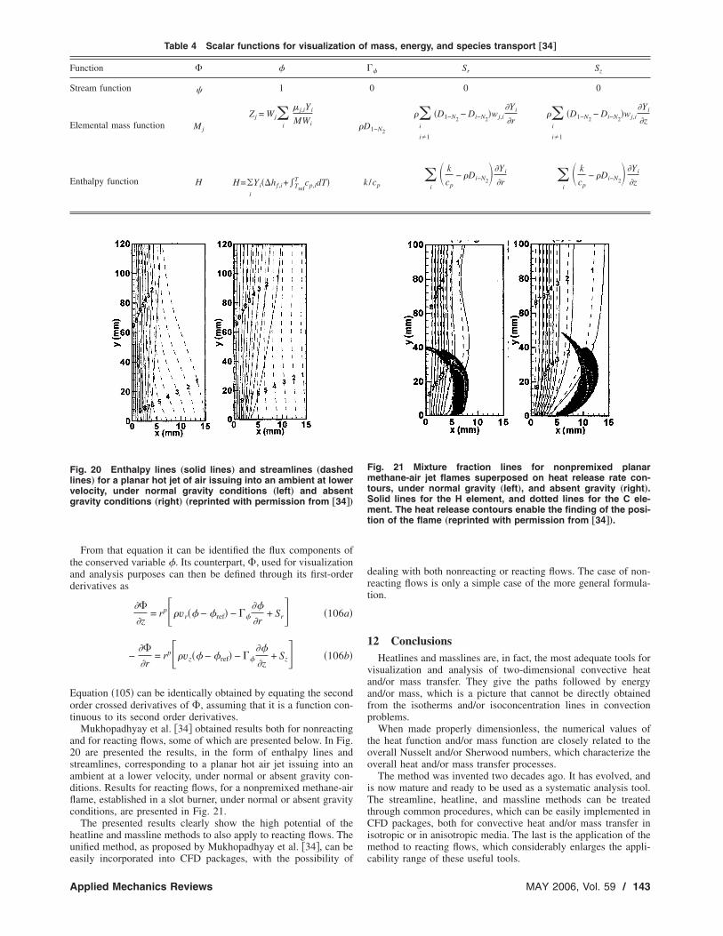
Mukhopadhyay et al. �34� obtained results both for nonreactingand for reacting flows, some of which are presented below. In Fig.20 are presented the results, in the form of enthalpy lines andstreamlines, corresponding to a planar hot air jet issuing into anambient at a lower velocity, under normal or absent gravity con-ditions. Results for reacting flows, for a nonpremixed methane-airflame, established in a slot burner, under normal or absent gravityconditions, are presented in Fig. 21.
The presented results clearly show the high potential of theheatline and massline methods to also apply to reacting flows. Theunified method, as proposed by Mukhopadhyay et al. �34�, can be
Table 4 Scalar functions for visualization
Function � �
Stream function � 1
Elemental mass function Mj
Zj = Wj�i
� j,iYi
MWi
Enthalpy function H H=�i
Yi��hf ,i+�Tref
T cp,idT�
Fig. 20 Enthalpy lines „solid lines… and streamlines „dashedlines… for a planar hot jet of air issuing into an ambient at lowervelocity, under normal gravity conditions „left… and absentgravity conditions „right… „reprinted with permission from †34‡…
easily incorporated into CFD packages, with the possibility of
Applied Mechanics Reviews
dealing with both nonreacting or reacting flows. The case of non-reacting flows is only a simple case of the more general formula-tion.
12 ConclusionsHeatlines and masslines are, in fact, the most adequate tools for
visualization and analysis of two-dimensional convective heatand/or mass transfer. They give the paths followed by energyand/or mass, which is a picture that cannot be directly obtainedfrom the isotherms and/or isoconcentration lines in convectionproblems.
When made properly dimensionless, the numerical values ofthe heat function and/or mass function are closely related to theoverall Nusselt and/or Sherwood numbers, which characterize theoverall heat and/or mass transfer processes.
The method was invented two decades ago. It has evolved, andis now mature and ready to be used as a systematic analysis tool.The streamline, heatline, and massline methods can be treatedthrough common procedures, which can be easily implemented inCFD packages, both for convective heat and/or mass transfer inisotropic or in anisotropic media. The last is the application of themethod to reacting flows, which considerably enlarges the appli-
mass, energy, and species transport †34‡
�� Sr Sz
0 0 0
1−N2
��i
i�1
�D1−N2− Di−N2
�wj,i�Yi
�r��
i
i�1
�D1−N2− Di−N2
�wj,i�Yi
�z
/cp�
i
� k
cp− �Di−N2
� �Yi
�r �i
� k
cp− �Di−N2
� �Yi
�z
Fig. 21 Mixture fraction lines for nonpremixed planarmethane-air jet flames superposed on heat release rate con-tours, under normal gravity „left…, and absent gravity „right….Solid lines for the H element, and dotted lines for the C ele-ment. The heat release contours enable the finding of the posi-tion of the flame „reprinted with permission from †34‡….
of
�D
k
cability range of these useful tools.
MAY 2006, Vol. 59 / 143
Nomenclature
A � surface areaC � mass fractioncp � constant pressure specific heatD � channel widthD � diffusion coefficient
Di−N2 � binary diffusion coefficient of species i in N2f � similarity functiong � auxiliary functiong � gravitational acceleration
grad � gradient vectorGr � grashof number
h � mixture enthalpyhi � enthalpy of species iH � heat function
i , j � unit Cartesian vectorsJe � energy flux vectorJm � mass flux vector
Jm,i � mass flux vector of chemical species iJ� � flux vector of �
k � thermal conductivityK � permeability
l ,m � director cosinesL � length
Le � Lewis numberM � mass functionm � mass flow raten � outward normal unit vectorN � buoyancy factor
Nu � Nusselt numberp � pressure
Pe � Péclet numberPr � Prandtl numberq� � heat flux
Q � heat flowr � radial coordinate �radial and spherical systems�
Ra � Rayleigh numberRe � Reynolds number
s � length segmentS � source termt � time
T � temperatureU � free stream or mean velocity
u ,v � Cartesian velocity componentswi,j � number of atoms of element element j
in species ix ,y � Cartesian coordinates
Y � mass fractionY � total heightz � longitudinal coordinateZ � elemental mass fraction
Greek Symbols� � thermal diffusivity� � volumetric expansion coefficient� � diffusion coefficient� � difference value � boundary layer thickness
�H � eddy diffusivity for heat� , � principal directions
� similarity variable� � tangential coordinate �cylindrical system�� � azimuthal coordinate �spherical system�� � dimensionless temperature� � dynamic viscosity
� ji � number of atoms of element j in 1 molecule
of species i144 / Vol. 59, MAY 2006
� � kinematic viscosity� � density� � generic variable� � generic variable, used for visualization� � stream function
SubscriptsB � at the boundaryC � cold wallH � hot walli � Chemical species i
L � based on length LQ � heat conductionr � radial
ref � reference point or reference valueT � thermal boundary layerw � at the wallxx � tensor component in the x directionxy � crossed tensor componentyy � tensor component in the y directionY � based on height Yz � longitudinal direction� � tangential or azimuthal direction� � generic variable� � generic variable0 � reference value� � free stream value* � dimensionless
Superscriptsp � index for coordinate system shifting
References�1� White, F. M., 1977, Viscous Fluid Flow, 2nd ed., McGraw-Hill, New York, p.
62.�2� Eckert, E. R. G., and Drake, R. M. Jr., 1972, Analysis of Heat and Mass
Transfer, McGraw-Hill, New York, Chap. 1.�3� Kimura, S., and Bejan, A., 1983, “The Heatline Visualization of Convective
Heat Transfer,” ASME J. Heat Transfer, 105, pp. 916–919.�4� Bejan, A., 1984, Convection Heat Transfer, Wiley, New York, pp. 21–23.�5� Trevisan, O. V., and Bejan, A., 1987, “Combined Heat and Mass Transfer by
Natural Convection in a Vertical Enclosure,” ASME J. Heat Transfer, 109, pp.104–112.
�6� Bello-Ochende, F. L., 1987, “Analysis of Heat Transfer by Free Convection inTilted Rectangular Cavities Using the Energy-Analogue of the Stream Func-tion,” Int. J. Mech. Eng. Education, 15�2�, pp. 91–98.
�7� Bello-Ochende, F. L., 1988, “A Heat Function Formulation for Thermal Con-vection in a Square Cavity,” Int. Commun. Heat Mass Transfer, 15, pp. 193–202.
�8� Oh, J. Y., Ha, M. Y., and Kim, K. C., 1997, “Numerical Study of Heat Transferand Flow of Natural Convection in an Enclosure With Heat-Generating Con-ducting Body,” Numer. Heat Transfer, Part A, 31, pp. 289–303.
�9� Costa, V. A. F., 1997, “Double-Diffusive Natural Convection in a Square En-closure With Heat and Mass Diffusive Walls,” Int. J. Heat Mass Transfer,40�17�, pp. 4061–4071.
�10� Deng, Q.-H., and Tang, G.-F., 2002, “Numerical Visualization of Mass andHeat Transport for Conjugate Natural Convection/Heat Conduction by Stream-line and Heatline,” Int. J. Heat Mass Transfer, 45�11�, pp. 2375–2385.
�11� Deng, Q.-H., and Tang, G.-F., 2002, “Numerical Visualization of Mass andHeat Transport for Mixed Convective Heat Transfer by Streamline and Heat-line,” Int. J. Heat Mass Transfer, 45�11�, pp. 2387–2396.
�12� Deng, Q.-H., Tang, G.-F., and Li, Y., 2002, “A Combined Temperature Scalefor Analyzing Natural Convection in Rectangular Enclosures With DiscreteHeat Sources,” Int. J. Heat Mass Transfer, 45�16�, pp. 3437–3446.
�13� Costa, V. A. F., 2004, “Double-Diffusive Natural Convection in Parallelogram-mic Enclosures Filled With Fluid-Saturated Porous Media,” Int. J. Heat MassTransfer, 47�12–13�, pp. 2699–2714.
�14� Morega, Al-M., 1988, “Magnetic Field Influence on the Convective HeatTransfer in the Solidification Processes, Part 2,” Rev. Roum. Sci. Tech.-Electrotech. et Energ., 33�2�, pp. 155–166.
�15� Morega, Al-M., 1988, “The Heat Function Approach to the ThermomagneticConvection of Electroconductive Melts,” Rev. Roum. Sci. Tech.-Electrotech.et Energ., 33�4�, pp. 359–368.
�16� Aggarwal, S. K., and Manhapra, A., 1989, “Use of Heatlines for UnsteadyBuoyancy-Driven Flow in a Cylindrical Enclosure,” ASME J. Heat Transfer,111, pp. 576–578.
�17� Aggarwal, S. K., and Manhapra, A., 1989, “Transient Natural Convection in a
Cylindrical Enclosure Nonuniformly Heated at the Top Wall,” Numer. HeatTransactions of the ASME
Transfer, Part A, 15, pp. 341–356.�18� Littlefield, D., and Desai, O., 1986, “Buoyant Laminar Convection in a Verti-
cal Cylindrical Annulus,” ASME J. Heat Transfer, 108, pp. 814–821.�19� Ho, C. J., and Lin, Y. H., 1989, “Thermal Convection Heart Transfer of Air/
Water Layers Enclosed in Horizontal Annuli With Mixed Boundary Condi-tions,” Waerme- Stoffuebertrag., 24, pp. 211–224.
�20� Ho, C. J., Lin, Y. H., Chen, T. C., 1989, “A Numerical Study of NaturalConvection in Concentric and Eccentric Horizontal Cylindrical Annuli WithMixed Boundary Conditions,” Int. J. Heat Fluid Flow, 10�1�, pp. 40–47.
�21� Ho, C. J., and Lin, Y. H., 1990, “Natural Convection of Cold Water in aVertical Annulus With Constant Heat Flux on the Inner Wall,” ASME J. HeatTransfer, 112, pp. 117–123.
�22� Chattopadhyay, H., and Dash, S. K., 1995, “Numerical Visualization of Con-vective Heat Transfer From a Sphere-With and Without Radial Mass Efflux,”Int. J. Numer. Methods Heat Fluid Flow, 5, pp. 705–716.
�23� Morega, Al. M., and Bejan, A., 1993, “Heatline Visualization of Forced Con-vection Laminar Boundary Layers,” Int. J. Heat Mass Transfer, 36�16�, pp.3957–3966.
�24� Morega, Al. M., and Bejan, A., 1994, “Heatline Visualization of Forced Con-vection in Porous Media,” Int. J. Heat Fluid Flow, 15�1�, pp. 42–47.
�25� Costa, V. A. F., 2000, “Heatline and Massline Visualization of the LaminarNatural Convection Boundary Layers Near a Vertical Wall,” Int. J. Heat MassTransfer, 43�20�, pp. 3765–3774.
�26� Dash, S. K., 1996, “Heatline Visualization in Turbulent Flow,” Int. J. Numer.Methods Heat Fluid Flow, 5�4�, pp. 37–46.
�27� Bejan, A., 1995, Convection Heat Transfer, 2nd ed., Wiley, New York.�28� Bejan, A., 2004, Convection Heat Transfer, 3rd ed., Wiley, New York.�29� Nield, D. A., and Bejan, A., 1999, Convection in Porous Media, 2nd ed.,
Springer, New York.
�30� Costa, V. A. F., 1999, “Unification of the Streamline, Heatline and MasslineApplied Mechanics Reviews
Methods for the Visualization of Two-Dimensional Transport Phenomena,” Int.J. Heat Mass Transfer, 42�1�, pp. 27–33.
�31� Costa, V. A. F., 2003, “Comment on the Paper by Qi-Hong Deng, Guang-FaTang, Numerical Visualization of Mass and Heat Transport for ConjugateNatural Convection/Heat Conduction by Streamline and Heatline,” IJHMT2002 45 �11� 2373-2385, Int. J. Heat Mass Transfer, 46�1�, pp. 185–187.
�32� Costa, V. A. F., 2003, “Unified Streamline, Heatline and Massline Methods forthe Visualization of Two-Dimensional Heat and Mass Transfer in AnisotropicMedia,” Int. J. Heat Mass Transfer, 46�8�, pp. 1309–1320.
�33� Mukhopadhyay, A., Qin, X., Aggarwal, and S. K., and Puri, I. K., 2002, “OnExtension of Heatline and Massline Concepts to Reacting Flows Through Useof Conserved Scalars,” ASME J. Heat Transfer, 124, pp. 791–799.
�34� Mukhopadhyay, A., Qin, X., Puri, I. K., and Aggarwal, S. K., 2003, “Visual-ization of Scalar Transport in Nonreacting and Reacting Jets Through a Uni-fied Heatline and Massline Formulation,” Numer. Heat Transfer, Part A, 44,pp. 683–704.
�35� Costa, V. A. F., 2004, “Visualization of Two-Dimensional Heat and MassTransfer Using the Heatlines and Masslines,” in Proceedings of the SymposiumBejan’s Constructal Theory of Shape and Structure, R. N. Rosa, A. H. Reis, A.F. Miguel, eds., Évora Geophysics Center, Évora, Portugal, Chap. 6, pp. 147–169.
�36� Gosman, D. A., Pun, W. M., Runchal, A. K., Spalding, D. B., and Wolfsthein,C. M., 1969, Heat and Mass Transfer in Recirculating Flows, Academic, NewYork.
�37� Slattery, J. C., 1999, Advanced Transport Phenomena, Cambridge UniversityPress, New York, pp. 50; 279–281.
�38� Davis, S. N., and DeWiest, R. J. M., 1966, Hydrogeology, Wiley, New York, p.197.
�39� Bear, J., 1979, Hydraulics of Groundwater, McGraw-Hill, New York, p. 102.
V. A. F. Costa is Associate Professor at the Universidade de Aveiro, Portugal. He received his M.Sc. andPh.D. in Mechanical Engineering (heat transfer branch) from the University of Coimbra (Portugal) in 1989and 1996, respectively. His main research and teaching activities include numerical heat transfer and fluidflow, convection heat transfer, engineering thermodynamics and drying. He uses several methods, includingcontrol volume finite element methods, with equal order interpolation for velocity and pressure. Some ofrecent work concerns the unification of the streamline, heatline, and massline methods, in order to havethem ready to be treated in a common basis and ease to be implemented in CFD packages. He is author orco-author of 20 refereed archival papers in journals, and 30 papers in refereed conference proceedings inthe aforementioned fields.
MAY 2006, Vol. 59 / 145