Beamforming Software Defined Radios for Wireless Sensor

Beamforming Software Defined Radios for Wireless SensorNetwork Interference Evaluation

William Zhao

Electrical Engineering and Computer SciencesUniversity of California at Berkeley

Technical Report No. UCB/EECS-2020-101http://www2.eecs.berkeley.edu/Pubs/TechRpts/2020/EECS-2020-101.html

May 29, 2020

Copyright © 2020, by the author(s).All rights reserved.

Permission to make digital or hard copies of all or part of this work forpersonal or classroom use is granted without fee provided that copies arenot made or distributed for profit or commercial advantage and that copiesbear this notice and the full citation on the first page. To copy otherwise, torepublish, to post on servers or to redistribute to lists, requires prior specificpermission.

Beamforming Software Defined Radios for Wireless Sensor Network Interference Evaluation

by

William J. Zhao

A thesis submitted in partial satisfaction of the

requirements for the degree of

Master of Science

in

Electrical Engineering and Computer Science

in the

Graduate Division

of the

University of California, Berkeley

Committee in charge:

Professor David E. Culler, ChairProfessor Prabal Dutta

Spring 2020


by William J. Zhao

Research Project

Submitted to the Department of Electrical Engineering and Computer Sciences, University of California at Berkeley, in partial satisfaction of the requirements for the degree of Master of Science, Plan II. Approval for the Report and Comprehensive Examination:

Committee:

Professor David E. Culler Research Advisor

5/26/2020

(Date)

* * * * * * *

Professor Prabal Dutta Second Reader

5/29/2020

(Date)

2


Copyright 2020by

William J. Zhao

1

Abstract


by

William J. Zhao

Master of Science in Electrical Engineering and Computer Science

University of California, Berkeley

Professor David E. Culler, Chair

Wireless communication on the 2.4GHz ISM band is becoming ever more prevalent in build-ings. Additionally, various physical layer technologies share this RF spectrum (e.g IEEE802.11 WiFi, Bluetooth, IEEE 802.15.4). As device density increases, devices sharing dif-ferent physical layer technologies will be forced to transmit on the similar frequencies aseach other, causing interference with each other’s transmissions. Low power wireless sensornetworks (WSN) utilizing IEEE 802.15.4 transmissions are particularly impacted by com-paratively high powered WiFi emissions. As a result, previous research work has been doneon network protocols to allow WSNs to mitigate the effect of cross-technology interference(CTI) produced from sources such as WiFi. However, the evaluation for these protocols dif-fer protocol to protocol including the method of WiFi interference generation. Many factorsthat affect the CTI observed by the WSN such as testbed layout, testbed container shape,CTI location, and antenna parameters makes it difficult to precisely adjust the levels of CTIon a WSN.

In order to provide a dynamic CTI generation platform that can be tuned to impact differentdevices within a WSN with different levels of interference, we develop a software defined ra-dio (SDR) solution. We propose Software Defined Interference Generation (SDIG) as a CTIgeneration method to induce WiFi CTI on motes instead of using real WiFi transceivers. No-tably SDIG uses an SDR array which allows beamforming techniques to steer the interferencesignal to impact different devices with varying magnitudes of interference.

We evaluate SDIG in comparison to real and arbitrarily placed CTI transmitters. We demon-strate the system’s ability to target individual nodes and deliver precise amounts of interfer-ence with minimal effects on other devices. However, we also reveal the scaling limitations ofusing SDIG to simultaneously impact many devices, each with varying amounts of interfer-ence. We recommend The use of beamforming in SDIG provides testbeds a way to carefullyinduce a level of CTI to a specific device within the testbed.

i

Contents

Contents i

List of Figures ii

List of Tables iv

1 Introduction 1

2 Related Works 3

3 System Architecture 43.1 Testbed Topology . . . . . . . . . . . . . . . . . . . . . . . . . . . . . . . . . 43.2 Software/Hardware Stack . . . . . . . . . . . . . . . . . . . . . . . . . . . . 53.3 Mote Bearing Coefficient Acquisition . . . . . . . . . . . . . . . . . . . . . . 63.4 Gain Coefficient Acquisition . . . . . . . . . . . . . . . . . . . . . . . . . . . 93.5 Multiplexed Interference Transmission . . . . . . . . . . . . . . . . . . . . . 10

4 Evaluation Results 124.1 WiFi Interference Performance . . . . . . . . . . . . . . . . . . . . . . . . . . 124.2 Single Transmitter Evaluation . . . . . . . . . . . . . . . . . . . . . . . . . . 154.3 Two Transmitter Evaluation . . . . . . . . . . . . . . . . . . . . . . . . . . . 184.4 Cross Channel Interference Performance . . . . . . . . . . . . . . . . . . . . 22

5 Development Challenges and Limitations Discussion 235.1 Bearing acquisition . . . . . . . . . . . . . . . . . . . . . . . . . . . . . . . . 235.2 Computational Demands of SDIG . . . . . . . . . . . . . . . . . . . . . . . . 245.3 Issues With Interference Multiplexing . . . . . . . . . . . . . . . . . . . . . . 25

6 Conclusion 26

Bibliography 28

ii

List of Figures

3.1 An abstract view of the network topology of the testbed. The main array con-troller has USB connections to each of the radios in the array. The ethernet-networked machines have JTAG connections to the motes to read debug infor-mation from the motes and to flash binaries to the motes. . . . . . . . . . . . . 5

3.2 An example of a top-down view of the testbed with 2 motes. Additionally, themotes and radios are all approximately on the same elevation. Various pieces offurniture are also present in this. . . . . . . . . . . . . . . . . . . . . . . . . . . 5

3.3 Top down view of transmitter array steering a signal by φ degrees. Steeringa signal to an angle φ will also result in a steered signal to −φ when only 2transmitters are used. . . . . . . . . . . . . . . . . . . . . . . . . . . . . . . . . 7

3.4 Phase driven beamforming array diagram. The beam is steered by phase shiftingantenna 1. This phase shift is done in software by multiplying the sample streamby the phase shift constant before it is sent to the radio. . . . . . . . . . . . . . 8

3.5 A top-down representation of the bearing sweep performed by the radio. . . . . 83.6 A block diagram representation of the gain coefficient acquisition subsystem. R is

the recorded energy from the mote when exposed to the real interference source.R’ is the measured gain coefficient from SDR array. x is the gain that the SDRarray is transmitting at. R’ changes over time as the difference between R andR’ is fed back into the system to nudge x to a value such that R = R’. . . . . . 10

3.7 GNU Radio flowgraph deployed to switch interference transmissions between twomotes. . . . . . . . . . . . . . . . . . . . . . . . . . . . . . . . . . . . . . . . . . 11

4.1 Energy reading histogram for mote 1 (left), and mote 2 (right) without explicitWiFi transmission over a period of 10 minutes. . . . . . . . . . . . . . . . . . . 13

4.2 Energy reading histogram for mote 1 (left), and mote 2 (right) with an explicithigh data rate WiFi transmission. The median readings are -51 and -71 dbm formotes 1 and 2 respectively. Energy readings were measured over 10 minutes. . . 13

4.3 Waterfall plot of channel 15 with an active high data rate transmission. Theheight of the waterfall represents 5 seconds of activity. The highlighted horizontalpurple streaks indicate periods of inactivity as the channel is empty for thattime period. The horizontal streaks of orange indicate periods of high activity.Although the channel is mostly active, there are numerous periods where thereis little activity. . . . . . . . . . . . . . . . . . . . . . . . . . . . . . . . . . . . 14

iii

4.4 Energy reading histogram for mote 1 (left) with 25 db baseband gain, and mote 2(right) with 27.6 db baseband gain. An explicit high data rate synthetic signal wasemitted. The median readings are -51 and -71 dbm for motes 1 and 2 respectively. 15

4.5 Waterfall plot of channel 15 with an active high data rate transmission from singletransmitter SDIG. The channel remains consistently active through throughoutthe capture. The height of the waterfall represents 5 seconds of activity. Com-pared to Figure 4.3, there is a distinct lack of horizontal purple streaks, indicatingthat the channel is consistently active. . . . . . . . . . . . . . . . . . . . . . . . 16

4.6 Observed energy detection plots from a sweep from 0 to π radians in 11 divisionsfor mote 1 (left) and mote 2 (right). Energy detection values were measured forone minute per division. In this case, the bearing was determined to be at π

2for

mote 1 (in front of the transmitter), and π10

for mote 2 (which is roughly to theright of the transmitter array). . . . . . . . . . . . . . . . . . . . . . . . . . . . 18

4.7 Observed energy readings for mote 1 and 2 when subject under 2 transmit-ter SDIG. Note how there are two peaks in each case which demonstrates thegain/bearing switching schema. . . . . . . . . . . . . . . . . . . . . . . . . . . . 20

4.8 New testbed topology. New furniture is added as well as 2 new motes. Thesemotes are connected to USB hubs which are in turn connected to a laptop. . . . 20

5.1 Estimation of mote bearing using gr-doa package. This method was ultimatelyscrapped since the data was too noisy to use. . . . . . . . . . . . . . . . . . . . 24

iv

List of Tables

4.1 PRR between mote 1 and mote 2 in our sample testbed over 30 minutes withno explicit WiFi interference, as well as with high data rate and low data rateinterference. . . . . . . . . . . . . . . . . . . . . . . . . . . . . . . . . . . . . . . 14

4.2 Evaluation of single transmitter SDIG for high and low data rate transmissions.Because a single transmitter is used, no beamforming can be done. (Mote x)means the transmitter is using the gain for Mote x. Switching indicates the datais taken when the transmitter is multiplexing between the gain values associatedwith mote 1 and 2. Bolded values are results from the mote that is properlycalibrated to the transmitter. Italicized values are result from the a mote that isreceiving packets from a mis-calibrated transmitter. . . . . . . . . . . . . . . . . 17

4.3 Evaluation of one and two transmitter SDIG. LDR stands for “low data rate”, andHDR stands for “high data rate”. A column with 1TX indicates a result measuredwith 1 SDR transmitter. A column with 2TX indicates a result measured with2 SDR transmitters. Bolded values are results from the mote that is properlycalibrated to the transmitter. Italicized values are result from the a mote that isreceiving packets from a mis-calibrated transmitter. . . . . . . . . . . . . . . . . 19

4.4 4 mote 2 transmitter SDIG system comparison to focused calibrated PRR com-pared to PRR with SDIG switching. . . . . . . . . . . . . . . . . . . . . . . . . 21

4.5 Comparison between the energy readings when subject to high data rate wirelesstraffic as well as high data rate SDIG interference from mote 1. . . . . . . . . . 22

v

Acknowledgments

I would like to thank the researchers in the BETS (Buildings, Energy, and TransportationSystems) research group for their contributions to the WSN software/hardware stack thatmy research heavily utilized. I especially want to thank Hyung-Sin Kim for his excellentmentorship and guidance through my entire research experience at BETS over the past fewyears which includes the work done for this thesis. I would also like to thank Professor DavidCuller for introducing this interesting problem space to me as well as providing critical insightand advice for this project. I would also like to thank Professor Prabal Dutta for being afaculty reviewer for this paper. Lastly, I want to acknowledge my family and peers who haveprovided knowledge and support these past years.

1

Chapter 1

Introduction

Starting from over a decade ago, we have noticed an incredible increase in the number ofwireless devices deployed [15]. Due to the limited bandwidth of the 2.4GHz unlicensed ISMband, devices sporting IEEE 802.11 (WiFi), Bluetooth, IEEE 802.15.4, and other formsof communication, all compete for connectivity in this band. Additionally, these devicescommunicate with varying levels of emission power and bandwidth. Due to the differentphysical properties of the transmissions, it’s not guaranteed that the radios across differenttransmission protocols can understand each other. This is particularly relevant for low powerwireless communication devices (which are used in the Internet of Things (IOT), homeautomation, and smart buildings) as such devices are constrained to be energy efficient.These devices cannot have high power transmitters and require a clear and reliable channelto transmit efficiently [9]. However, due to increase in the density of wireless devices, lowpower devices deployed in wireless sensor networks (WSN) are heavily impacted by otherwireless transmitters due to frequency exhaustion. Transmissions from higher power devicessuch as WiFi overshadow the transmit strength of devices in WSNs (motes). Performance ofWSNs are impacted so much from cross technology interference (CTI) that research work andnetwork stacks for WSNs to mitigate CTI has been developed. Some mitigation strategiesinclude having motes dodge the interference entirely while others involve the motes accuratelypredicting intervals in which it’s probable for a transmission to succeed in a crowded channel[8, 11, 12, 21].

When comparing the performance of CTI mitigation protocols, packet reception ratio(PRR) is one of the main metrics of determining the success of the protocol. By limitingthe amount of re-transmissions a mote has to make before a packet is proliferated throughthe network, the power efficiency of the mote increases. One of the main parameters tunedto evaluate PRR in an environment with interference generators is the distance the motesare from the generator. As the motes are placed further from the source of interference,the received “signal” becomes weaker due to propagation. A valid method of emulating theeffect of an interference source being further way is to transmit using a lower gain in the firstplace [9].

Despite this degree of freedom for evaluation through transmit gain adjustment, it’s

CHAPTER 1. INTRODUCTION 2

still difficult to sculpt motes to receive particular levels of attenuation just by adjustingthe transmit gain. Suppose we have a system with one interference generation source, oneomni-directional antenna, and two motes that are placed equidistant to the omnidirectionalantenna on opposite sides. Barring multipath effects, it would be impossible for the omni-directional antenna to induce different levels of observed interference on the motes.

This problem can be addressed through the use of a multi-antenna array. By construc-tively and destructively combining a target signal in a direction through spaced apart anten-nas, known as beamforming, a transmission array can impose different levels of interferenceon motes that are equidistant from the array but have different bearings. In order to accu-rately beamform a signal, tight synchronization between the signals transmitted across theantennas is necessary. This is non-trivial with off the shelf wireless transceivers. However, inthe past decade, an increasingly popular technology, known as software defined radios, havebeen shown to achieve synchronization to allow for beamforming without too much trouble.

Software defined radios (SDRs) with transmit capabilities can generally take in-phaseand quadrature samples from a machine, upshift them to a target carrier frequency, andtransmit the results over the air. Alternatively, SDRs can be used to receive samples at atarget carrier frequency, and convert the results to IQ (in-phase, quadrature) samples to beprocessed in software. This is incredibly powerful as software toolchains such as GNU Radiocan be used to rapidly prototype routines to send and receive packets [4]. Additionally, theseradios can be synchronized, making them a perfect candidate to perform beamforming.

In order to be able to better evaluate WSN performance with varying network stacks,we suggest an architecture known as Software Defined Interference Generation (SDIG) as away to tune and emulate the WiFi interference experienced by motes in an arbitrary testbedenvironment.

3

Chapter 2

Related Works

SDRs have been utilized to emulate the radio stack for a multitude of wireless protocolsincluding WiFi and IEEE 802.15.4 for both transmit and receive purposes. GNU Radio isalso shown to be a staple tool used in the SDR community for many research and industrialapplications [21, 10, 11, 14].

SDRs have been shown to be particularly useful in testbed deployments as a way to verifythe correctness of other hardware receivers [14]. Additionally, they have even been used asthe means of executing CTI mitigation strategies due to the ability to quickly prototype theentire protocol in software and arbitrarily deploy it to radios [9]. Most relevantly, SDRs havebeen used as a useful means of generating CTI in testbeds themselves. In these experiments,CTI is produced using radio stacks such as WiFi in order to evaluate CTI mitigation protocolswhere signal demodulation is important [10].

Beamforming has also been successfully used in SDR applications as well. However, inthese cases, the beamformed signal was designed to be received and demodulated to mitigateinterference rather than impart interference on a device [13].

We expand on the work done on using SDRs as a CTI source by utilizing beamforming as away to induce varying levels of interference on motes in a testbed without being constrained tothe testbed topology and environment. No currently known work explicitly uses beamformingas a way to tune the levels of CTI that motes receive in a deployment.

4

Chapter 3

System Architecture

We propose SDIG (Software Defined Interference Generation) as the interference generationsystem to emulate WiFi interference for motes.

Deploying SDIG in any capacity requires the use of multiple calibration steps with feed-back from the motes in the testbed. The main parameters that need to be obtained are themote bearing with respect to the SDR array as well as the correct gain to transmit to theradio.

The steps involved to deploy SDIG are as follows:

1. Acquire calibration coefficients

a) Acquire the transmit direction value for each mote.

b) Acquire the transmission gain values required for the SDR array to match theobserved interference from the true WiFi source at each mote.

2. Transmit a synthetic beamformed WiFi pattern, repeatedly switching the steeringdirection and transmit gain of the array in time to impact each mote.

3.1 Testbed Topology

Our testbed consists of the SDR array, the radio array controller machine, wireless motes,ethernet-networked machines with debuggers attached to the motes, and the interferencegenerator. The networked machines are also part of the same wired network as the arraycontroller machine. These do not necessarily have to be part of the same network as thesample interference source, but this is the case in our testbed. Figures 3.1 and 3.2 show anabstract and physical representation of our sample testbed.

During some tests, various objects were introduced to introduce multipath effects into thesystem. Motes were also moved around/introduced to the system. The arrays were placedapproximately 0.25 meters apart from each other which is approximately the distance of 2wavelengths at the transmit carrier frequency.

CHAPTER 3. SYSTEM ARCHITECTURE 5

Figure 3.1: An abstract view of the network topology of the testbed. The main arraycontroller has USB connections to each of the radios in the array. The ethernet-networkedmachines have JTAG connections to the motes to read debug information from the motesand to flash binaries to the motes.

Figure 3.2: An example of a top-down view of the testbed with 2 motes. Additionally, themotes and radios are all approximately on the same elevation. Various pieces of furnitureare also present in this.

3.2 Software/Hardware Stack

For our SDR array, we used 2 HackRF devices as our SDR choice [7]. These were affixed toa table. In the naive case, even if we transmit on both HackRFs, the transmitted samples


can be offset by thousands of samples which would not be suitable for beamforming. Tomitigate this drift, we had our first HackRF be a master device and the second HackRF bea slave device. The slave device utilizes the clock from the master. We also made sure thateach HackRF shared a common ground. This synchronization procedure has been previouslyconducted and is documented in the HackRF wiki [16]. Each SDR was connected a desktopmachine via USB which could run the radio flowgraphs to perform calibration and generateinterference.

Our testbed mainly used two Hamilton motes running RIOT-OS with the GNRC networkstack [1, 18]. TelosB motes running Contiki-NG with the RPL network stack were also usedfor an experiment [3]. When measuring the energy readings in the air, the Hamilton mote’sradio has a register which outputs the “energy level” at a channel. This value evaluatesthe average energy level over 8 symbol periods. For the TelosB motes, the RSSI value istaken from the radio. A laptop and Raspberry Pi were responsible for reading the debuginformation from the motes as well as forwarding the data to the desktop machine [17].

For both the Hamilton mote and the TelosB mote, two binaries were developed: onethat repeatedly yields the energy reading/RSSI on a channel and udp client/server binary inwhich the client mote periodically sends packets carrying a sequence number to the receiver.

A WiFi dongle was used to generate interference. UDP packets were sent over the airthrough an access point to a wired device on the network.

To control the SDR array, we used GNU Radio, a signal processing toolkit which allowsthe use and development of signal processing blocks to control signals. We heavily utilizedan open-source 802.11 module which allows the generation of WiFi packets [5].

3.3 Mote Bearing Coefficient Acquisition

For deployments with greater than 1 transmitter, beamforming a signal to a mote requiresthe mote’s bearing in order to steer the signal in the right direction. It should be notedthat although traditional beamforming systems are complex and can adjust the transmitweights dynamically, our system’s motes have coarse granularity and are static throughoutthe calibration and test process. Thus, our bearing detection algorithm for our 2 lineartransmitter system involves sweeping the bearing space. For a given desired angle to beamtowards, we can phase shift the signal for one of our transmitters by the following expression:

ejm(2πdλcos(φ)) (3.1)

In our implementation, m is the transmitter number, d is the distance in meters betweentransmitters, λ is the wavelength of the transmission frequency, and φ is defined by the angleto steer the signal.

In our system, having only 2 transmitters is not sufficient to completely disambiguatethe steering direction in 360 degrees. A signal steered φ degrees is also steered −φ degrees asthe cosine in equation 3.1 would evaluate to the same value as well as because the antennas


are omni-directional. This is illustrated in Figure 3.3. The steering is done in software bymultiplying a sample stream by the phase offset as shown in Figure 3.4.

Figure 3.3: Top down view of transmitter array steering a signal by φ degrees. Steering asignal to an angle φ will also result in a steered signal to −φ when only 2 transmitters areused.

Thus, we only need to consider the angles between 0 and π radians. We first flash a bi-nary to the mote under calibration which allows it to report its energy reading/RSSI valuesover the debug interface. We obtain the steering direction for each mote by arbitrarily steer-ing the high rate synthetic WiFi transmission in different directions, recording the observedenergy reading from the mote, and then taking the argmax of the result. An example oftested directions can be found in Figure 3.5. The gain used in both transmitters are the sameand is set high enough to register above the noise floor on the motes. However, because ofthe limited resolution from mote (the measurements are in dbm), the dynamic range of thesweep is rather limited. Nevertheless, this strategy does yield the best bearing to the nearestdbm from evaluation. An example result of a frequency sweep is illustrated in Figure 4.6.

We obtain the best bearing for each mote in the test using this method.


Figure 3.4: Phase driven beamforming array diagram. The beam is steered by phase shiftingantenna 1. This phase shift is done in software by multiplying the sample stream by thephase shift constant before it is sent to the radio.

Figure 3.5: A top-down representation of the bearing sweep performed by the radio.


3.4 Gain Coefficient Acquisition

In order to evaluate the transmission (tx) gain that the SDR array should be using tobeamform to the mote, it’s important to see how the mote reacts to the original interferencesource. The mote is first flashed with the binary which allows energy readings to be outputto the debug interface. The mote is then subjected to a high data rate transfer from theWiFi interference source. This is to ensure that a large percentage of the energy readingsamples are taken when the transmitter is transmitting. Once the interference source istransmitting, we start sampling the mote’s energy readings. After sufficient samples arecollected, the median reading is taken to get the target energy reading to achieve with theSDR array.

If we are using more than 1 transmitter, we first load the bearing derived earlier into oursynthetic WiFi transmission program . We then start transmitting a high data rate syntheticWiFi interference to that specific mote with an arbitrary gain that is higher than the noisefloor for the calibrated mote. A service on the networked machines that are connected to themotes then reads the energy readings and serve them to any requester. Meanwhile, a logicblock running on the SDR array controller requests samples from the networked machinesattached to the mote. An averaging filter, designed to reduce the effect of noise on the controlfeedback system, consumes the samples. The difference between the target energy readingand the observed energy reading is then scaled by a gain constant (Ki) and added currentTX gain to generate the new TX gain. This continues until the target energy reading is meton the mote or the SDR array saturates. Note that since this is a pure integral controller, thegain will likely never converge completely, but will slightly oscillate around the correct TXgain value. The feedback system is terminated whenever the energy readings have settledaround the target. The TX gain value is then saved. Essentially, this system is just anauto gain control system which seeks to find the the right transmit gain to achieve the sameenergy reading that the real interference source achieved on the mote. A diagram of thefeedback control system can be shown in Figure 3.6.

We obtain the best SDR TX gain for each mote in the test using this method.


Figure 3.6: A block diagram representation of the gain coefficient acquisition subsystem. Ris the recorded energy from the mote when exposed to the real interference source. R’ is themeasured gain coefficient from SDR array. x is the gain that the SDR array is transmittingat. R’ changes over time as the difference between R and R’ is fed back into the system tonudge x to a value such that R = R’.

3.5 Multiplexed Interference Transmission

Once the TX gain and bearing values for each mote have been calibrated, SDIG can bedeployed. When a variable data rate synthetic transmission is being sent, the gains andbearing are switched periodically so that the signal is optimized for a different mote at anygiven time. This is achieved in software by generating a separate ramp function between thevalues of -1 and 1 at an arbitrary frequency of 1000Hz which serves as as a pseudo-timer toswitch the gain and bearing weights in time. Adjusting the frequency parameter will notaffect the fraction of the time a particular mote will be focused on. For a two mote testbed,the radio will transmit with the gain and bearing for mote 0 when the ramp function isbetween -1 and 0, and transmit with the gain and bearing for mote 1 otherwise. This canbe extended to more motes by further dividing the intervals in the ramp function further.The GNU Radio flowgraph used to transmit the signal at these bearings and gains is shownin Figure 3.7.

This concludes the setup and deployment of SDIG.


Figure 3.7: GNU Radio flowgraph deployed to switch interference transmissions between twomotes.

12

Chapter 4

Evaluation Results

4.1 WiFi Interference Performance

Accurately controlling the physical bits sent over the WiFi NIC in time is non-trivial, so it isimportant to understand how transmissions manifest themselves in the physical layer. Usingthe testbed topology described in Figure 3.2 (where mote 1 is the mote closer to the SDRarray as well as the WiFi interference source), we evaluated the effect of WiFi interferenceon a 2 Hamilton mote sensor network.

The WiFi access point was configured to transmit on WiFi channel 4 (2427 MHz centerfrequency). The motes were configured to evaluate the energy readings tuned to 802.15.4channel 15 (2425 MHz center frequency). These channels were chosen as they had theleast amount of traffic. Choosing an empty channel is extremely important as exogenousinterference induces confounding effects on our calibration results. For our high data ratetransmission, a program was created to repeatedly pipe in 1500 “x” characters over the airvia netcat. For our low data transmission, the program would repeatedly pipe in 200 “x”characters with a 5 millisecond break between transmissions.

We first obtained a control result by evaluating the “empty” channel 15. The moteslistened to the channel for 10 minutes and recorded the energy readings over this. Figure 4.1shows a histogram of the results. The lowest value that can be read by the mote is -94dbmand this result dominates most of the energy reading samples for both motes. This is to beexpected as the channel is “empty” in this instance.

We then transmitted using the true interference source and performed a similar energyreading measurement. Figure 4.2 shows a histogram of the results. As expected, the medianreading of mote 1 is higher than mote 2 as mote 1 is closer physically to the transmitter.Interesting enough, around 5% of the samples were low energy readings even with the ag-gressive transmission. This brought up the question about whether the transmission itselfwas rendered as a bursty signal or whether the transmission was rendered as a sustainedtransmission over the air.

After generating a waterfall graph of the spectral density over time on 802.15.4 channel

CHAPTER 4. EVALUATION RESULTS 13

Figure 4.1: Energy reading histogram for mote 1 (left), and mote 2 (right) without explicitWiFi transmission over a period of 10 minutes.

Figure 4.2: Energy reading histogram for mote 1 (left), and mote 2 (right) with an explicithigh data rate WiFi transmission. The median readings are -51 and -71 dbm for motes 1and 2 respectively. Energy readings were measured over 10 minutes.

15, we observed that this high data rate transmission did indeed have significant holes inthe transmission in which the channel goes empty (shown in Figure 4.3). We were not ableto completely eliminate these regions of inactivity with netcat.

We then evaluate the packet reception ratio from mote 1 to mote 2 and vice versa underno interference, high data rate interference, and low data rate interference. When evaluatingmote 1’s PRR (packet reception ratio), we had mote 2 send UDP packets with an embeddedsequence number every 0.1 seconds to mote 1 while mote 1 was listening. It should be notedthat we sent packets using the GNRC network stack. Similarly, to measure mote 2’s PRR,


Figure 4.3: Waterfall plot of channel 15 with an active high data rate transmission. Theheight of the waterfall represents 5 seconds of activity. The highlighted horizontal purplestreaks indicate periods of inactivity as the channel is empty for that time period. Thehorizontal streaks of orange indicate periods of high activity. Although the channel is mostlyactive, there are numerous periods where there is little activity.

we simply swapped which mote was sending and which was receiving. To estimate PRR inthis scenario, we looked at the most recently observed sequence number and divided it by thetotal amount of packets received. The results are shown in Table 4.1. As expected, the PRRof the motes while under little CTI is near perfect. When the high data rate interference issent, PRR plummets greatly. We also observed that Mote 2’s PRR is significantly higher inboth the low data rate experiment as well as the high data rate experiment. This is almostcertainly due to the fact that mote 2 is significantly further from the interference sourcecompared to mote 1.

Interference Type Mote 1 PRR Mote 2 PRR

None 99.9% 99.9%Low Data Rate WiFi 67.6% 75.9%High Data Rate WiFi 1.2% 5.0%

Table 4.1: PRR between mote 1 and mote 2 in our sample testbed over 30 minutes with noexplicit WiFi interference, as well as with high data rate and low data rate interference.


4.2 Single Transmitter Evaluation

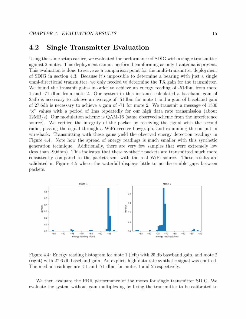
Using the same setup earlier, we evaluated the performance of SDIG with a single transmitteragainst 2 motes. This deployment cannot perform beamforming as only 1 antenna is present.This evaluation is done to serve as a comparison point for the multi-transmitter deploymentof SDIG in section 4.3. Because it’s impossible to determine a bearing with just a singleomni-directional transmitter, we only needed to determine the TX gain for the transmitter.We found the transmit gains in order to achieve an energy reading of -51dbm from mote1 and -71 dbm from mote 2. Our system in this instance calculated a baseband gain of25db is necessary to achieve an average of -51dbm for mote 1 and a gain of baseband gainof 27.6db is necessary to achieve a gain of -71 for mote 2. We transmit a message of 1500“x” values with a period of 1ms repeatedly for our high data rate transmission (about12MB/s). Our modulation scheme is QAM-16 (same observed scheme from the interferencesource). We verified the integrity of the packet by receiving the signal with the secondradio, passing the signal through a WiFi receive flowgraph, and examining the output inwireshark. Transmitting with these gains yield the observed energy detection readings inFigure 4.4. Note how the spread of energy readings is much smaller with this syntheticgeneration technique. Additionally, there are very few samples that were extremely low(less than -90dbm). This indicates that these synthetic packets are transmitted much moreconsistently compared to the packets sent with the real WiFi source. These results arevalidated in Figure 4.5 where the waterfall displays little to no discernible gaps betweenpackets.

Figure 4.4: Energy reading histogram for mote 1 (left) with 25 db baseband gain, and mote 2(right) with 27.6 db baseband gain. An explicit high data rate synthetic signal was emitted.The median readings are -51 and -71 dbm for motes 1 and 2 respectively.

We then evaluate the PRR performance of the motes for single transmitter SDIG. Weevaluate the system without gain multiplexing by fixing the transmitter to be calibrated to


Figure 4.5: Waterfall plot of channel 15 with an active high data rate transmission fromsingle transmitter SDIG. The channel remains consistently active through throughout thecapture. The height of the waterfall represents 5 seconds of activity. Compared to Figure 4.3,there is a distinct lack of horizontal purple streaks, indicating that the channel is consistentlyactive.

only mote at a time. We then evaluate single transmitter with gain switching. For each ofthese data points, we observe the PRR over 15 minutes. The results of this experiment isdescribed in Table 4.2.

If we compare the correctly calibrated results for mote 1 and mote 2, we see a discrepancyin results when compared to the PRR observed with the real interference source. Particularly,when examining the high data rate transfers, we observe that the PRR for both motes 1and 2 are under 1% when calibrated for each mote whereas the PRR in the real interferencecase is 1.2 and 5% respectively. This is most likely due to the fact that the actual WiFiinterference source is more bursty (refer to Figure 4.3) than the packets being transmittedfrom the SDR. When evaluating the low data rate performance, even though both the realinterference source and the synthetic interference source were sending approximately thesame data at the same rate, the synthetic data yielded a lower PRR for both motes (60.5%verses 67.6%, and 70.5% vs 75.9%). A similar theory explaining this discrepancy is how the“on-time” of the transmitters differ between the generators.

When looking at the off-calibrated results, we see a significant change in PRR. Becausethe transmission gain for mote 1 is lower than that of mote 2, we see that PRR for mote2 increases significantly when transmitted with mote 1’s gain (79.8% vs 70.5% for mote 2).Similarly, we see that mote 1’s performance drops significantly when it’s subject to mote 2’s


Interference Type Mote 1 PRR Mote 2 PRR

None 100% 100%Low Data Rate WiFi 67.6% 75.9%High Data Rate WiFi 1.2% 5.0%

Low Data Rate 1TX SDIG (Mote 1) 60.5% 79.8%Low Data Rate 1TX SDIG (Mote 2) 55.9% 70.5%Low Data Rate 1TX SDIG (Switching) 58.9% 76.3%High Data Rate 1TX SDIG (Mote 1) 0.5% 1.2%High Data Rate 1TX SDIG (Mote 2) 0.35% 0.83%High Data Rate 1TX SDIG (Switching) 0.46% 0.93%

Table 4.2: Evaluation of single transmitter SDIG for high and low data rate transmissions.Because a single transmitter is used, no beamforming can be done. (Mote x) means thetransmitter is using the gain for Mote x. Switching indicates the data is taken when thetransmitter is multiplexing between the gain values associated with mote 1 and 2. Boldedvalues are results from the mote that is properly calibrated to the transmitter. Italicizedvalues are result from the a mote that is receiving packets from a mis-calibrated transmitter.

transmit gain (55.9% vs 60.5%) as mote 2’s transmission gain is higher than that of mote1. When gain switching is enabled, we observe an averaging of the PRR performance fromthe calibrated and off-calibrated result. In the case of mote 1, the new PRR is worse thanthe PRR with the calibrated transmitter. For mote 2, the new PRR is better than the PRRwith the calibrated transmitter.

Some key insights to takeaway from this experiment is that SDIG with 1 transmitter,even when calibrated to the correct mote, our payload can’t perfectly replicate the PRR fora sample interference load from a real transmitter. This is due to the fact that the activetime of the transmitter differs from that of the real transmitter. Because the physical layersignal is created at software level, this can be finely controlled and adjusted for future work.Additionally, we observe that gain switching achieves an undesirable averaging effect for themotes. Motes that are closer to the transmit array will see significantly worse PRRs than itscalibration PRR and motes further from the transmit array will notice better PRRs. Thismakes a single transmitter deployment of SDIG undesirable for emulating interference at anarbitrary location. Even when independently trying to interfere with a target node, due tothe lack of beamforming, the non-targeted mote is impacted significantly as well. This isdemonstrated clearly when Mote 1’s PRR becomes worse when the device is targeting mote2 which means more interference is being detected by mote 1.


4.3 Two Transmitter Evaluation

Using the same setup used before, with the exception of the second transmitter turned on,we evaluated the performance of SDIG with a two transmitters against 2 motes. To sanitycheck the energy detection readings, we first transmitted the same high data rate syntheticpayload and same gain value used in the single transmitter evaluation for mote 1 to bothtransmitters and measured the observed energy detection on mote 1 (which is in front of thearray, so π/2 bearing). Unsurprisingly, we observed a 3dbm increase in the energy reading,which roughly corresponds to a 2 times increase in energy presence which makes sense as wesimply doubled our transmit capabilities.

We then run the bearing coefficient acquisition scheme to acquire the bearings for themotes. The results of the sweep are displayed in Figure 4.6.

Figure 4.6: Observed energy detection plots from a sweep from 0 to π radians in 11 divisionsfor mote 1 (left) and mote 2 (right). Energy detection values were measured for one minuteper division. In this case, the bearing was determined to be at π

2for mote 1 (in front of the

transmitter), and π10

for mote 2 (which is roughly to the right of the transmitter array).

We then ran the gain coefficient acquisition scheme for each mote to calibrate the trans-mitters to achieve the correct energy readings that were observed in the true WiFi inter-ference experiment. Note that we preload the appropriate bearing when calibrating themote. Once we have achieved all the vectors, we evaluated a couple PRR measurements.We observed the PRR from motes 1 and 2 when we: beamform to only mote 1, beamformto only mote 2, and multiplexed between beamforming to mote 1 and mote2. The resultsare described in Table 4.3.

From these results we see that when the transmitters are calibrated to the motes, theresults from the calibrated motes in the single transmitter and two transmitter case arepretty consistent. However, as expected, the off calibration results are significantly different.Though, in the case mote 1, its results weren’t as impacted compared to the single transmittercase. Even though a higher gain is used to beamform to mote 2, because the bearing is


Interference Type Mote 1 PRR 1TX Mote 1 PRR 2TX Mote 2 PRR 1TX Mote 2 PRR 2TX

LDR (Mote 1) 60.5% 61.1% 79.8% 84.3%LDR (Mote 2) 55.9% 59.2% 70.5% 68.5%LDR (Switching) 58.9% 60.4% 76.3% 78.5%HDR (Mote 1) 0.5% 0.52% 1.2% 5.3%HDR (Mote 2) 0.35% 0.47% 0.83% 0.4%HDR (Switching) 0.46% 0.49% 0.93% 1.2%

Table 4.3: Evaluation of one and two transmitter SDIG. LDR stands for “low data rate”,and HDR stands for “high data rate”. A column with 1TX indicates a result measuredwith 1 SDR transmitter. A column with 2TX indicates a result measured with 2 SDRtransmitters. Bolded values are results from the mote that is properly calibrated to thetransmitter. Italicized values are result from the a mote that is receiving packets from amis-calibrated transmitter.

significantly different, the net negative effect on the PRR for mote 1 is diminished comparedto that of the single transmitter case. In the case of mote 2, the off calibration result showsa drastic improvement in PRR as not only is the TX gain less, but also the bearing is outof alignment, which reduces the negative impact of the transmitter. This demonstrates thatwe are able to minimally impact other motes when we are targeting a particular mote.

In general, in comparison to the single transmitter switching, the 2 transmitter switchingsystem yields higher PRR in each case. It is apparent that the performance disparity betweenthe switching and non-switching schemes comes from the fact that the system can currentlyspend a fraction of its time beamforming to one mote a time. This is observed from themote in Figure 4.7.

We further tested the limitations of multiplexing the signal by calibrating the system to4 motes. We introduced two TelosB motes into the testbed. Additional objects were alsoadded to the testbed which introduced multipaths during this experiment. Figure 4.8 showsthe new topology of the testbed. RSSI readings were pulled from the radio on the TelosBmotes and were used to calibrate the gains. Additionally, communication between the moteswere strictly Hamilton mote to Hamilton mote and TelosB mote to TelosB mote. The TelosBmotes also transmitted on 802.15.4 channel 15.

We performed a low-data rate deployment of SDIG against these 4 motes. We multiplexedthe gain/bearing parameters 4-way to each of the devices during transmission. The resultsare summarized in Table 4.4. As we can see, the PRR discrepancy between calibrated resultand switching result is amplified as we add more motes. This shows that one of the mainlimitations of this schema is the fact that as more motes are added, the less time the systemhas to satisfy the interference demand of the mote.


Figure 4.7: Observed energy readings for mote 1 and 2 when subject under 2 transmitterSDIG. Note how there are two peaks in each case which demonstrates the gain/bearingswitching schema.

Figure 4.8: New testbed topology. New furniture is added as well as 2 new motes. Thesemotes are connected to USB hubs which are in turn connected to a laptop.


Interference Type Hamilton 1 PRR Hamilton 2 PRR TelosB 1 PRR TelosB 2 PRR

LDR Calibrated PRR 64.3% 78% 63.4% 66.5%LDR Switching PRR 72.3% 91.3% 77.2% 82.7%

Table 4.4: 4 mote 2 transmitter SDIG system comparison to focused calibrated PRR com-pared to PRR with SDIG switching.


4.4 Cross Channel Interference Performance

We also tested how the energy readings for a different 802.15.4 channel would compare whensubject to a 2 transmitter SDIG deployment calibrated to channel 15 verses the actual wire-less interference transmission. We calibrated our deployment to channel 15 for a single moteand updated energy reading binary on the mote to display the energy readings for channels14 to 17. We then exposed the mote to interference from the actual WiFi interference sourceas well as 2 transmitter SDIG deployment. The results are shown in Table 4.5. As it turnsout, the calibrated gains only hold well for channels close to the center frequency of the WiFichannel. Although channel 14 and 17 are normally impacted by traffic on wireless channel 4,they aren’t as impacted as hard in the SDIG deployment. This phenomenon may be relevantif SDIG were to be deployed to a multi-channel testbed, however, this was not evaluated.

Channel WiFi Interference 2 TX SDIG Calibrated

14 -50 -6715 -51 -5116 -52 -5217 -54 -72

Table 4.5: Comparison between the energy readings when subject to high data rate wirelesstraffic as well as high data rate SDIG interference from mote 1.

23

Chapter 5

Development Challenges andLimitations Discussion

In this section, we discuss technical implementation challenges that were experienced inevaluating or developing SDIG.

5.1 Bearing acquisition

Before settling on the beamforming scheme illustrated in chapter 3, additional developmentattempts were made to attempt to create a more elegant bearing calculation algorithm.

In the initial draft of SDIG, instead of performing a bearing sweep, a direction of arrivalalgorithm was proposed as a way of obtaining the bearing. A binary for the motes wasdeveloped to cause it to periodically transmit a signal. In this configuration, the SDR arraywas set to receive the 802.15.4 packet from each transmitter and based off the differences inthe received signal on each antenna from each radio, a bearing can be produced. This wouldideally eliminate the need for an exhaustive search.

The initial proposed method of determining the bearing involves listening for the start ofthe 802.15.4 packet on both transmitters, evaluating the time of arrival for each transmitter,and, based off the difference in arrival (DOA), perform some trigonometry to figure outbearing. The time difference would be determined through cross correlation between theradios. However, after some preliminary analysis, we deemed that the resolution of thistechnique is not sufficient. Assuming both motes were receiving at 10 megasamples persecond and perfect synchronization between radios, if radio 1 received the packet 1 samplebefore radio 2, that would mean that the received signal propagated 100 nanoseconds longerbefore being received. Given the speed of light in a vacuum, this method would only yield aresolution of 30 meters per sample which is way too coarse. Thus, a time difference approachfor direction of arrival is not feasible.

Another approach for deriving the bearing involved using PCA on the measured readingsto determine the best bearing, also known as the Capon method [2]. This approach was

CHAPTER 5. DEVELOPMENT CHALLENGES AND LIMITATIONS DISCUSSION 24

originally implemented as an open source module in GNU Radio for the RTL-SDR [19]. Weattempted to proceed with this method for measuring DOA. In the sample flowgraph, theSDRs will be synchronized via cross-correlation, the phase difference between the receivedsignals would be filtered, and an arc-cosine function is used to output the correct angle.We ported this module to GNU Radio 3.8 and adapted the example DOA flowgraph touse the HackRF sources instead of the RTL-SDR sources. However, we were not able toachieve significant results using this method as the measurements were too noisy. Figure 5.1illustrates the noisy performance of this method when transmitting 802.15.4 packets. Wetried changing the packet length to see if it could be processed properly through the modulebut with limited success. The original use of this module was to identify the source of a usertransmitting using a walkie talkie, so perhaps this package was not particularly compatiblethe modulation scheme used in 802.15.4.

Figure 5.1: Estimation of mote bearing using gr-doa package. This method was ultimatelyscrapped since the data was too noisy to use.

We also considered implementing the MUSIC algorithm to satisfy the DOA acquisition[6]. However, after obtaining preliminary results with the bearing sweep experiment, animplementation of MUSIC was ultimately not implemented. That being said, performingDOA analysis in an environment with multipaths through extensions of the MUSIC algorithmis not only possible, but has been shown to be accurate to the decimeter level [20]. Futurework that refines the beamforming procedure should utilize these more elegant methods ofDOA.

5.2 Computational Demands of SDIG

In the first high data rate deployment of SDIG, the system would stop functioning properlyafter a few seconds. This resulted in the radios not transmitting anything at all. Thisissue was not observed when generating packets with a high periodicity. Ultimately, it wasobserved that our machine could not keep up with the real time demand of constructing,tagging, and modulating the packets when the period between the packets is incredibly low.In order to resolve this issue, we generated the complex sample signatures for a few high

CHAPTER 5. DEVELOPMENT CHALLENGES AND LIMITATIONS DISCUSSION 25

data rate packets and saved these results to a file. When performing high data rate SDIG,we instead transmit packets from this file repeatedly rather than going through the motionsof generating each bit of the packet. Although we sent the same payload every time in ourlow data rate and high data rate tests, further work involving random messages may havetrouble generating random packets at a high enough rate if repeated samples cannot be sent.

5.3 Issues With Interference Multiplexing

As demonstrated in the 2 and 4 mote demonstration of 2 transmitter SDIG, when thetransmitters start multiplexing the transmissions to different motes, each mote only directlyreceives interference for a fraction of the transmission duration. This leads to an overall in-crease in PRR as the motes will register the channel impacted less often. This fundamentallylimits the scalability of motes that SDIG can service in a testbed. To illustrate this, considerthe ideal example where we have n motes and a perfect beamforming array barring multi-path effects such that only 1 mote receives interference at all at any time instance. Assumingthat each mote is fairly served interference, that would mean that the mote would only everreceive interference 1

nof the time. Assuming packets are received properly when there’s no

interference and no packets can be achieved when there is interference, the expected PRRper mote in this ideal system would then be n−1

n.

26

Chapter 6

Conclusion

In this paper, we present the design and implementation of software defined interferencegeneration system against wireless sensor networks without prior knowledge of channel in-formation. By developing a simple energy detection binary for each mote architecture, SDIGcan be used to calibrate its steering angle as well as transmit gain to emulate the perfor-mance of a real wireless transmitter that is located elsewhere on motes located throughouta testbed. We also demonstrate consistency issues when it comes to using a real wirelesstransmitter as an interference source. This issue is not observed using SDIG. We believe themote performance discrepancy is mostly due to the difference in transmission consistencybetween the true WiFi interference source and SDIG. We show that through the use of mul-tiple antennas and beamforming, we are able to somewhat prevent unnecessary interferencelevels from impacting other motes as well. Finally, we reveal the scaling limitations of SDIGby demonstrating its inability to match the performance of a focused transmission when itmultiplexes its signal to various motes. Our use of the radio is fundamentally different fromthat of emitting a signal designed to persist through a channel; we generate noise designed tomatch the effects of the channel from a different source. Ultimately, one of the realizations ofthis experiment was that providing high fidelity control of interference over a WSN is ratherdifficult without compromising on either the scalability or the flexibility of the of the systemcompared to generating an explicit signal.

One way to potentially scale the system is by deploying multiple transmitter arrays toserve a larger number of motes in a testbed. This method is quite expensive as the cost ofa single software defined radio with transmit capabilities costs on the order of hundreds ofdollars. Furthermore, more computing resources would be needed to drive these radios aswell.

Nevertheless, a single deployment SDIG can serve as an invaluable evaluation system onits own in a testbed as its physical interference signature can easily be defined and configuredin software to impact a particular spot in space. For instance, a single deployment of amulti-transmitter SDIG can test the effect of an intermittently active mote within a WSNby compromising its receive capabilities. Different interference types (e.g 2.4GHz microwaveradiation, 802.15.4 packets, etc), different bearings, and various transmit gain coefficients can

CHAPTER 6. CONCLUSION 27

all be defined in software. Additionally, the utilization of flow-graphs created in GNU Radioallows interference generation patterns/signatures to be built and shared across differentdeployments and testbeds. This potentially enables remote testbeds to support a widespectrum of CTI signatures.

28

Bibliography

[1] Michael P Andersen, Hyung-Sin Kim, and David E Culler. “Hamilton: a cost-effective,low power networked sensor for indoor environment monitoring”. In: Proceedings ofthe 4th ACM International Conference on Systems for Energy-Efficient Built Environ-ments. 2017, pp. 1–2.

[2] Jack Capon. “High-resolution frequency-wavenumber spectrum analysis”. In: Proceed-ings of the IEEE 57.8 (1969), pp. 1408–1418.

[3] Contiki-NG, the Next Generation Contiki. url: https://github.com/contiki-

ng/contiki-ng.

[4] GNU Radio Website. url: http://www.gnuradio.org.

[5] GR-IEEE80211. IEEE 802.11 a/g/p transceiver. url: https://github.com/bastibl/gr-ieee802-11.

[6] P. Gupta and S. P. Kar. “MUSIC and improved MUSIC algorithm to estimate di-rection of arrival”. In: 2015 International Conference on Communications and SignalProcessing (ICCSP). 2015, pp. 0757–0761.

[7] HackRF. url: https://github.com/mossmann/hackrf.

[8] Anwar Hithnawi, Hossein Shafagh, and Simon Duquennoy. “TIIM: technology-independentinterference mitigation for low-power wireless networks”. In: Proceedings of the 14thInternational Conference on Information Processing in Sensor Networks. 2015, pp. 1–12.

[9] Anwar Hithnawi, Hossein Shafagh, and Simon Duquennoy. “Understanding the im-pact of cross technology interference on IEEE 802.15. 4”. In: Proceedings of the 9thACM international workshop on Wireless network testbeds, experimental evaluationand characterization. 2014, pp. 49–56.

[10] Anwar Hithnawi et al. “Controlled Interference Generation for Wireless CoexistenceResearch”. In: Proceedings of the 2015 Workshop on Software Radio ImplementationForum. 2015, pp. 19–24.

[11] Anwar Hithnawi et al. “Crosszig: combating cross-technology interference in low-powerwireless networks”. In: 2016 15th ACM/IEEE International Conference on InformationProcessing in Sensor Networks (IPSN). Ieee. 2016, pp. 1–12.

BIBLIOGRAPHY 29

[12] Song Min Kim and Tian He. “Freebee: Cross-technology communication via free side-channel”. In: Proceedings of the 21st Annual International Conference on Mobile Com-puting and Networking. 2015, pp. 317–330.

[13] A. Krdu et al. “Beamforming for interference mitigation and its implementation onan SDR baseband processor”. In: 2011 IEEE Workshop on Signal Processing Systems(SiPS). 2011, pp. 192–197.

[14] S. G. Ku, H. S. Lim, and A. W. C. Tan. “A software defined radio testbed for simulationand real-world testing of RF subsampling receiver”. In: International Conference onFrontiers of Communications, Networks and Applications (ICFCNA 2014 - Malaysia).2014, pp. 1–6.

[15] FCC Lab. “Report on Trends in Wireless Devices.” In: (2011). url: www.fcc.gov/oet/info/documents/reports/wirelessdevices.doc.

[16] Multiple device hardware level synchronization. url: https://github.com/mossmann/hackrf/wiki/Multiple-device-hardware-level-synchronization#upgrade.

[17] Raspberry Pi. url: https://www.raspberrypi.org/.

[18] RIOT - The friendly OS for IoT. url: https://github.com/RIOT-OS/RIOT.

[19] Todd Moon Sam Whiting Dana Sorensen. “Direction of Arrival Analysis on a MobilePlatform”. GR Con 17. 2017. url: https://www.gnuradio.org/grcon/grcon17/presentations/real-time_direction_finding/Todd-Moon-Gnuradio-DOA.pdf.

[20] Elahe Soltanaghaei, Avinash Kalyanaraman, and Kamin Whitehouse. “Multipath tri-angulation: Decimeter-level wifi localization and orientation with a single unaided re-ceiver”. In: Proceedings of the 16th annual international conference on mobile systems,applications, and services. 2018, pp. 376–388.

[21] X. Zhang and K. G. Shin. “Gap Sense: Lightweight coordination of heterogeneouswireless devices”. In: 2013 Proceedings IEEE INFOCOM. 2013, pp. 3094–3101.

Documents

Beamforming Software Defined Radios for Wireless Sensor