Embed Size (px)
Citation preview

Beam Scattering Effects- Simulation Tools Developed at The APS
A. Xiao and M. Borland
Mini-workshop on Dynamic Aperture Issues of USR
Nov. 12, 2010

2
Motivation A future light source requires:
– Ultra low emittance beam– High particle density
High quality beam is strongly affected by scattering processes:– Small angle scattering: IBS effect – emittance dilution in all dimensions.
• IBS growth rate – Bjorken-Mtingwa's (BM) formula
– Large angle scattering: Touschek effect – particle loss.• Piwinski's formula – Arbitrary beam shape and energies
Beam scattering effects seriously limit achievable machine performance!
with
with
(for )

3
Example: PEP-X
PEP-X: “A Design Report of the baseline for PEP-X: anUltra-Low Emittance Storage Ring,” SLAC-PUB-13999

Concerns for a Linac-Based 4th Generation Light Source
The beam scattering effects in ERL are comparable to or more severe than in the APS.
The formula need to be updated to handle energy variation (e.g., acceleration).
The Linac beam has non-Gaussian profile.
Particle distribution from optimized high-brightness injector simulation
Provided by X. Dong
RERLRAPS
∝1.×F / 2ERL F /2APS
1/ t d ERL1/ t d APS
∝185×G / ERLG /APS

5
Simulation Tools Developed at the APS
Able to simulate:– Beam scattering effects with energy variation– A non-Gaussian distributed bunch
Simulation tools added to elegant– For both Gaussian and non-Gaussian distributed bunch– Applicable to ring and linac tracking– IBSCATTER: Intra-beam scattering– TSCATTER: Touschek-scattering
External simulation tools– Simplified versions of above tools
• Use data typically provided by elegant
– Only for Gaussian distributed bunch– ibsEmittance – applicable to ring+linac– touschekLifetime – applicable to ring only

Beam Scattering with Energy Variation
The beamline is divided into small sections by inserting special elements IBSCATTER (IBS) or TSCATTER (Touschek) in the beamline.
The scattering rates are calculated locally using normalized beam parameters and integrated over each section.
At each IBSCATTER:– The beam size is enlarged according to the calculated scattering rate by modifying
tracking particles coordinates.– New beam parameters are used for the following section's simulation.
At each TSCATTER:– A bunch of scattered particles are generated using Monte-Carlo simulation, each
representing part of the integrated scattering rate.– Scattered particles are tracked, loss rate and loss position are recorded.
… …
ISCATTER or TSCATTER
&insert_elements name = *, type = *[QSB]*, skip = 1, element_def = "TS0: TSCATTER",&end

Simulation of Touschek Effect Well known effect in storage ring
– Single Coulomb scattering process.– Small transverse momentum → large longitudinal momentum.– Main cause of short lifetime for low-emittance, high-charge bunches
Approaches to lifetime computation– Bruck's formula
• Flat beam, non-relativistic transverse momentum
– Piwinski's formula• Arbitrary beam shape and energy• Local scattering rate using local optical functions and momentum aperture• Preferred over Bruck's formula, used in elegant and touschekLifetime
– Monte-Carlo simulation• Gives loss distribution• Not necessary for lifetime computation

Lifetime computation with touschekLifetime Only applicable to Gaussian-distributed stored beam. Required input
– Twiss parameter file from elegant– Momentum aperture file from elegant– Bunch parameter
• charge, coupling, bunch length – required• Emittance, dp/p – optional
Output– Lifetime– Local scattering rate R
Example touschekLifetime -twiss=aps.twi -aperture=aps.mmap aps.life \ -charge=15 -coupling=0.01 -length=12

Touschek Scattering Simulation – overview
&touschek_scatterdouble charge = 0;double frequency = 1;double emit_nx = 0;double emit_ny = 0;double sigma_dp = 0;double sigma_s = 0;STRING Momentum_Aperture = NULL;STRING FullDist = NULL;STRING TranDist = NULL;long n_simulated = 5E6;double ignored_portion = 0.01;long i_start = 0;long i_end = 1;long do_track = 0;STRING output = NULL;...
&end

Calculate Local Bunch Distribution Function By default assumes a Gaussian bunch For non-Gaussian bunch, use SDDS-based histogram table
– Given by user from measurement or tracking– For tracking, an MHISTOGRAM element is required to be inserted in front of every
TSCATTER element.
Input can be either– 3 x 2D: need Xdist + Ydist + Zdist;– 2D+4D: need TranDist + Zdist; (Used in our example)– 6D: need FullDist;
• ideal but need large population of simulated input bunch for getting meaningful distribution function.
Index: n sub-index counter:Long. - [NsNp]
Tran. - [NxNxpNyNyp]
11
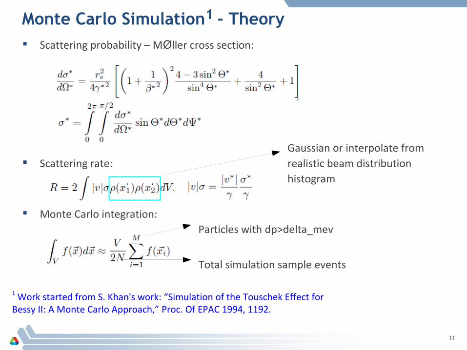
Monte Carlo Simulation1 - Theory Scattering probability – MØller cross section:
Scattering rate:
Monte Carlo integration:
Gaussian or interpolate fromrealistic beam distribution histogram
Particles with dp>delta_mev
Total simulation sample events
1 Work started from S. Khan's work: “Simulation of the Touschek Effect for Bessy II: A Monte Carlo Approach,” Proc. Of EPAC 1994, 1192.
12
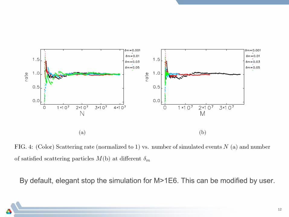
By default, elegant stop the simulation for M>1E6. This can be modified by user.
13

14
Monte Carlo Simulation – non-Gaussian beam
At η=0, Piwinski's rate does not depend on input energy spread At η≠0, Piwinski's rate depends on input energy spread, so results are un-reliable
for linac bunch. Need real bunch distribution for calculation.

15
Simulation of Beam Loss Rate and Position
Scattered particles from Monte Carlo simulation are collected and tracked from the scattering location to the end of beamline (linac) or multiple tunes (storage ring).
Each scattered particle represents scattering rate of:
Particle loss position and associated scattering rate are saved.
Total number of simulated scattered particles are M x NTS
Ri=ri
∑ ri∫l RP ds×
RMCRP

16
Speed up Simulation Simulated scattering particles don't present same probability. Most of them are
rare events.
For efficient tracking, we only track those with high probability. What we care is the loss rate and loss position.
– The ignored part are particle's with large momentum deviation, and very likely, they are lost immediately after scattering.
– The relative simulation error will be ignored portion divided by the loss portion of tracked particles. For example if 50% (rate) tracked particles lost and the ignored portion is 1%, the relative simulation error is 2%.
– Try to use delta_mev close to the simulated momentum aperture as input (for example: 80%).
18% for 99.9% scattering!
Tracked
17
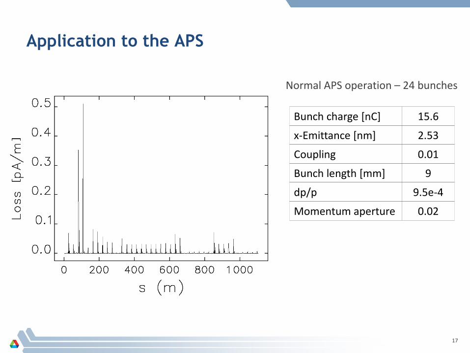
Application to the APS
Normal APS operation – 24 bunches
Bunch charge [nC] 15.6
x-Emittance [nm] 2.53
Coupling 0.01
Bunch length [mm] 9
dp/p 9.5e-4
Momentum aperture 0.02
18
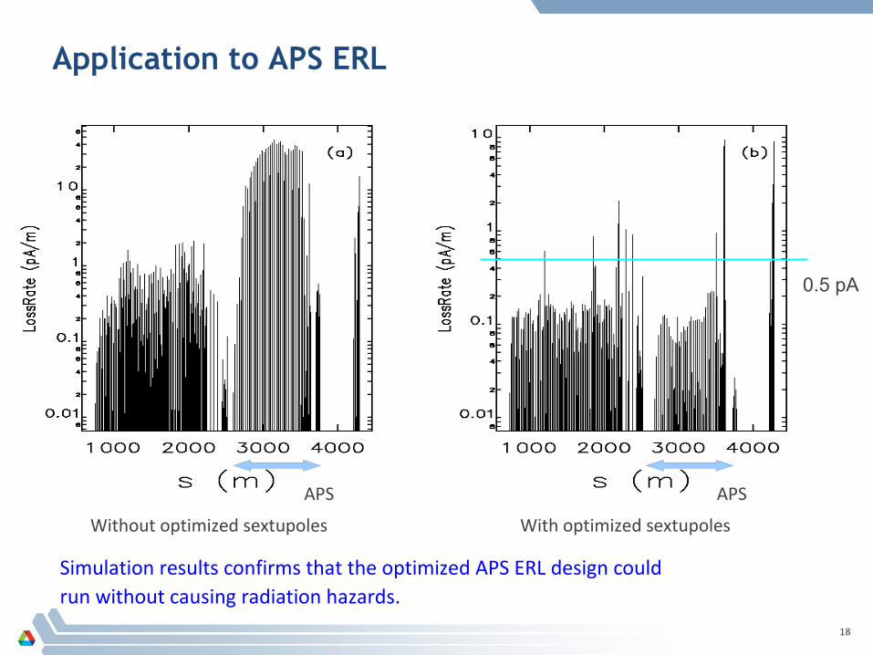
Application to APS ERL
APS APS
Without optimized sextupoles With optimized sextupoles
0.5 pA
Simulation results confirms that the optimized APS ERL design couldrun without causing radiation hazards.

19
IBS Simulation
The nature of IBS and Touschek effect are different– We care more beam size evolution than the real particle distribution.– The beam size dilution need time to develop
• Requires fewer ISCATTER element – only needed when beam size has a noticeable change.
For Gaussian bunch, use ibsEmittance or IBSCATTER– Bjorken-Mtingwa's (BM) formula: Vertical dispersion effect is included.
IbsEmittance– Input
• Twiss file from elegant• Beam parameters – charge, coupling, bunch length
– Output• Emittance evaluation• Local growth rate at given beam parameters
Example:
ibsEmittance aps.twi aps.out -charge=15 -coupling=0.01 -length=10 \
-integrate=turns=50000,step=300
ibsEmittance aps.twi aps.out -charge=15 -coupling=0.01 -length=10 -growth

20

21
IBS Simulation for Non-Gaussian Bunches
For non-Gaussian beams, use tracking with IBSCATTER elements– Slice technique important for photo-injector beams
Procedures:– Bunch is sliced at the beginning of each section of the beamline.– The IBS growth rates are calculated using BM formula for each slice, assuming particles
in slice are Gaussian-distributed in (x,x',y,y',δ) and uniformly distributed in longitudinal.– Particle coordinates are modified based on the calculated growth rate (smoothly or
randomly).– Particles from each slice are mixed and reform a new bunch. This bunch is ready for the
simulation of next section.

22
IBS – Growth Rate for Sliced and Unsliced Beam
1 nC, 1 µm normalized emittance.
LCLS: 63.5 MeV to 4.4 GeV APS-ERL: 10 MeV to 7 GeV

23
IBS – Simulated Beam Property

24
IBS – Bunch Energy Spread Evolution

25
Example of using command line tools with elegant
Task: evaluate APS stored beam performance as a function of energy Tools:
– elegant: compute nominal equilibrium properties vs energy– haissinski: compute bunch length for specific bunch charge vs energy, using
data from elegant– ibsEmittance: compute energy spread and emittance using results from
elegant and haissinski– touscheckLifetime: compute Touschek lifetime using results from
ibsEmittance, haissinski, and elegant– sddsbrightness: compute brightness tuning curves using data from
ibsEmittance and elegant– sddsfluxcurve: compute flux tuning curves using data from ibsEmittance and
elegant Command line tools are readily scripted for fast turn-around

26
Results of energy scan

27
Results of energy scan using optimized superconducting undulators
The “GoodEnough” parametershows how many photonenergies within the25-100 keV band can beprovided with brightnessthat is within a factor 2 ofthe best achievable. Forconservative magnetic gap,> 7 GeV is preferred.
Gap

28
Conclusion
Tools to simulate beam scattering effects for both stored and linac beam with energy variation are developed
– Command line tools for quick, accurate ring evaluation– Features in elegant for more fundamental simulation
Beam loss rate and position information can be obtained precisely from Monte Carlo simulation using a realistic beam distribution.
Beam size evaluation is obtained by applying the Bjorken-Mtingwa formula to a sliced bunch.
Application results to an example APS ERL lattice show:– The Touschek scattering effects is significant.
• The momentum aperture needs to be optimized carefully.• A beam collimation system can be designed based on the result.
– The IBS growth rate is much higher compared to a normal stored beam• Traveling time is very short – IBS effect has no enough time to develop. • No obvious effect on the machine's performance.
Command line tools are very useful for ring design studies

29
Acknowledgment
We would like to express our special thank to S. Khan for his original work on Monte Carlo simulation of Touschek effect.
We also followed F. Zimmerman's work to include vertical dispersion to the IBS calculation.
During the development, we had many useful discussions with L. Emery.


![arXiv:physics/0612252v2 [physics.optics] 30 Dec 2006incident beam). The scattering force is obtained in the Rayleigh-Gans approximation, in terms of extinction and scattering efficiencies](https://img.pdfslide.us/doc/110x75/60b8a7be49a5ab20320ab8a3/arxivphysics0612252v2-30-dec-2006-incident-beam-the-scattering-force-is.jpg)