LCLS-TN-12-1

Beam Pipe Corrector Study

Zachary Wolf, Yurii LevashovSLAC

March 19, 2012

Abstract

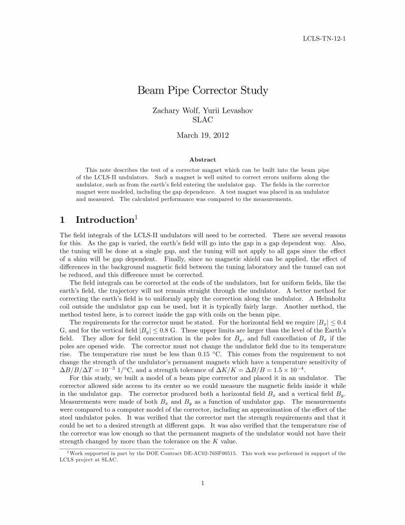
This note describes the test of a corrector magnet which can be built into the beam pipeof the LCLS-II undulators. Such a magnet is well suited to correct errors uniform along theundulator, such as from the earth�s �eld entering the undulator gap. The �elds in the correctormagnet were modeled, including the gap dependence. A test magnet was placed in an undulatorand measured. The calculated performance was compared to the measurements.

1 Introduction1

The �eld integrals of the LCLS-II undulators will need to be corrected. There are several reasonsfor this. As the gap is varied, the earth�s �eld will go into the gap in a gap dependent way. Also,the tuning will be done at a single gap, and the tuning will not apply to all gaps since the e¤ectof a shim will be gap dependent. Finally, since no magnetic shield can be applied, the e¤ect ofdi¤erences in the background magnetic �eld between the tuning laboratory and the tunnel can notbe reduced, and this di¤erence must be corrected.The �eld integrals can be corrected at the ends of the undulators, but for uniform �elds, like the

earth�s �eld, the trajectory will not remain straight through the undulator. A better method forcorrecting the earth�s �eld is to uniformly apply the correction along the undulator. A Helmholtzcoil outside the undulator gap can be used, but it is typically fairly large. Another method, themethod tested here, is to correct inside the gap with coils on the beam pipe.The requirements for the corrector must be stated. For the horizontal �eld we require jBxj � 0:4

G, and for the vertical �eld jByj � 0:8 G. These upper limits are larger than the level of the Earth�s�eld. They allow for �eld concentration in the poles for By, and full cancellation of Bx if thepoles are opened wide. The corrector must not change the undulator �eld due to its temperaturerise. The temperature rise must be less than 0:15 �C. This comes from the requirement to notchange the strength of the undulator�s permanent magnets which have a temperature sensitivity of�B=B=�T = 10�3 1=�C, and a strength tolerance of �K=K = �B=B = 1:5� 10�4.For this study, we built a model of a beam pipe corrector and placed it in an undulator. The

corrector allowed side access to its center so we could measure the magnetic �elds inside it whilein the undulator gap. The corrector produced both a horizontal �eld Bx and a vertical �eld By.Measurements were made of both Bx and By as a function of undulator gap. The measurementswere compared to a computer model of the corrector, including an approximation of the e¤ect of thesteel undulator poles. It was veri�ed that the corrector met the strength requirements and that itcould be set to a desired strength at di¤erent gaps. It was also veri�ed that the temperature rise ofthe corrector was low enough so that the permanent magnets of the undulator would not have theirstrength changed by more than the tolerance on the K value.

1Work supported in part by the DOE Contract DE-AC02-76SF00515. This work was performed in support of theLCLS project at SLAC.

1

In practice, it is envisioned that a beam pipe corrector will be used to set the second �eld integralsof both Bx and By to zero. This will keep the beam trajectories maximally straight. A secondcorrection, such as by moving the quadrupole at the exit end of the undulator, will be used tocompensate for any residual �rst �eld integral from the undulator.

2 Test Corrector Design

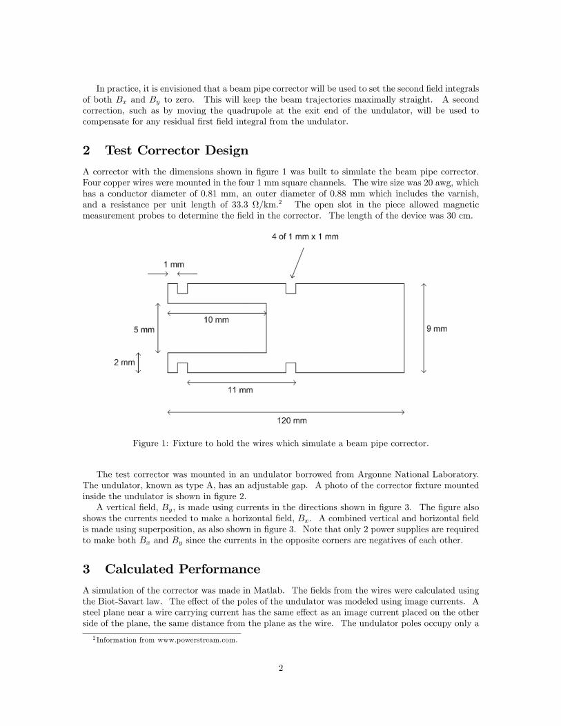
A corrector with the dimensions shown in �gure 1 was built to simulate the beam pipe corrector.Four copper wires were mounted in the four 1 mm square channels. The wire size was 20 awg, whichhas a conductor diameter of 0:81 mm, an outer diameter of 0:88 mm which includes the varnish,and a resistance per unit length of 33:3 =km.2 The open slot in the piece allowed magneticmeasurement probes to determine the �eld in the corrector. The length of the device was 30 cm.

Figure 1: Fixture to hold the wires which simulate a beam pipe corrector.

The test corrector was mounted in an undulator borrowed from Argonne National Laboratory.The undulator, known as type A, has an adjustable gap. A photo of the corrector �xture mountedinside the undulator is shown in �gure 2.A vertical �eld, By, is made using currents in the directions shown in �gure 3. The �gure also

shows the currents needed to make a horizontal �eld, Bx. A combined vertical and horizontal �eldis made using superposition, as also shown in �gure 3. Note that only 2 power supplies are requiredto make both Bx and By since the currents in the opposite corners are negatives of each other.

3 Calculated Performance

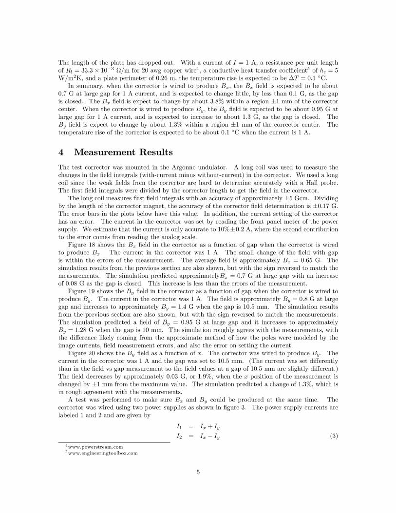
A simulation of the corrector was made in Matlab. The �elds from the wires were calculated usingthe Biot-Savart law. The e¤ect of the poles of the undulator was modeled using image currents. Asteel plane near a wire carrying current has the same e¤ect as an image current placed on the otherside of the plane, the same distance from the plane as the wire. The undulator poles occupy only a

2 Information from www.powerstream.com.

2

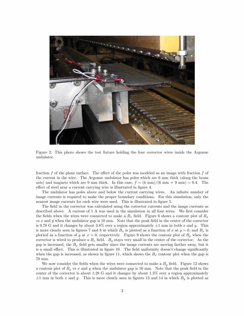
Figure 2: This photo shows the test �xture holding the four corrector wires inside the Argonneundulator.

fraction f of the plane surface. The e¤ect of the poles was modeled as an image with fraction f ofthe current in the wire. The Argonne undulator has poles which are 6 mm thick (along the beamaxis) and magnets which are 9 mm thick. In this case, f = (6 mm)=(6 mm + 9 mm) = 0:4. Thee¤ect of steel near a current carrying wire is illustrated in �gure 4.The undulator has poles above and below the current carrying wires. An in�nite number of

image currents is required to make the proper boundary conditions. For this simulation, only thenearest image currents for each wire were used. This is illustrated in �gure 5.The �eld in the corrector was calculated using the corrector currents and the image currents as

described above. A current of 1 A was used in the simulation in all four wires. We �rst considerthe �elds when the wires were connected to make a Bx �eld. Figure 6 shows a contour plot of Bxvs x and y when the undulator gap is 10 mm. Note that the peak �eld in the center of the correctoris 0:78 G and it changes by about 3:8% over a region approximately �1 mm in both x and y. Thisis more clearly seen in �gures 7 and 8 in which Bx is plotted as a function of x at y = 0, and Bx isplotted as a function of y at x = 0, respectively. Figure 9 shows the contour plot of By when thecorrector is wired to produce a Bx �eld. By stays very small in the center of the corrector. As thegap is increased, the Bx �eld gets smaller since the image currents are moving farther away, but itis a small e¤ect. This is illustrated in �gure 10. The �eld uniformity doesn�t change signi�cantlywhen the gap is increased, as shown in �gure 11, which shows the Bx contour plot when the gap is70 mm.We now consider the �elds when the wires were connected to make a By �eld. Figure 12 shows

a contour plot of By vs x and y when the undulator gap is 10 mm. Note that the peak �eld in thecenter of the corrector is about 1:28 G and it changes by about 1:3% over a region approximately�1 mm in both x and y. This is more clearly seen in �gures 13 and 14 in which By is plotted as

3

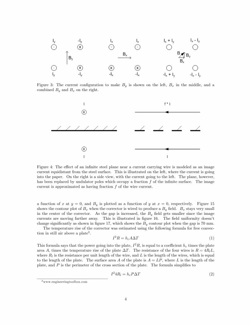
Figure 3: The current con�guration to make By is shown on the left, Bx in the middle, and acombined By and Bx on the right.

Figure 4: The e¤ect of an in�nite steel plane near a current carrying wire is modeled as an imagecurrent equidistant from the steel surface. This is illustrated on the left, where the current is goinginto the paper. On the right is a side view, with the current going to the left. The plane, however,has been replaced by undulator poles which occupy a fraction f of the in�nite surface. The imagecurrent is approximated as having fraction f of the wire current.

a function of x at y = 0, and By is plotted as a function of y at x = 0, respectively. Figure 15shows the contour plot of Bx when the corrector is wired to produce a By �eld. Bx stays very smallin the center of the corrector. As the gap is increased, the By �eld gets smaller since the imagecurrents are moving farther away. This is illustrated in �gure 16. The �eld uniformity doesn�tchange signi�cantly as shown in �gure 17, which shows the By contour plot when the gap is 70 mm.The temperature rise of the corrector was estimated using the following formula for free convec-

tion in still air above a plate3 .I2R = hcA�T (1)

This formula says that the power going into the plate, I2R, is equal to a coe¢ cient hc times the platearea A, times the temperature rise of the plate �T . The resistance of the four wires is R = 4RlL,where Rl is the resistance per unit length of the wire, and L is the length of the wires, which is equalto the length of the plate. The surface area A of the plate is A = LP , where L is the length of theplate, and P is the perimeter of the cross section of the plate. The formula simpli�es to

I24Rl = hcP�T (2)

3www.engineeringtoolbox.com

4

The length of the plate has dropped out. With a current of I = 1 A, a resistance per unit lengthof Rl = 33:3� 10�3 =m for 20 awg copper wire4 , a conductive heat transfer coe¢ cient5 of hc = 5W/m2K, and a plate perimeter of 0:26 m, the temperature rise is expected to be �T = 0:1 �C.In summary, when the corrector is wired to produce Bx, the Bx �eld is expected to be about

0:7 G at large gap for 1 A current, and is expected to change little, by less than 0:1 G, as the gapis closed. The Bx �eld is expect to change by about 3:8% within a region �1 mm of the correctorcenter. When the corrector is wired to produce By, the By �eld is expected to be about 0:95 G atlarge gap for 1 A current, and is expected to increase to about 1:3 G, as the gap is closed. TheBy �eld is expect to change by about 1:3% within a region �1 mm of the corrector center. Thetemperature rise of the corrector is expected to be about 0:1 �C when the current is 1 A.

4 Measurement Results

The test corrector was mounted in the Argonne undulator. A long coil was used to measure thechanges in the �eld integrals (with-current minus without-current) in the corrector. We used a longcoil since the weak �elds from the corrector are hard to determine accurately with a Hall probe.The �rst �eld integrals were divided by the corrector length to get the �eld in the corrector.The long coil measures �rst �eld integrals with an accuracy of approximately �5 Gcm. Dividing

by the length of the corrector magnet, the accuracy of the corrector �eld determination is �0:17 G.The error bars in the plots below have this value. In addition, the current setting of the correctorhas an error. The current in the corrector was set by reading the front panel meter of the powersupply. We estimate that the current is only accurate to 10%�0:2 A, where the second contributionto the error comes from reading the analog scale.Figure 18 shows the Bx �eld in the corrector as a function of gap when the corrector is wired

to produce Bx. The current in the corrector was 1 A. The small change of the �eld with gapis within the errors of the measurement. The average �eld is approximately Bx = 0:65 G. Thesimulation results from the previous section are also shown, but with the sign reversed to match themeasurements. The simulation predicted approximatelyBx = 0:7 G at large gap with an increaseof 0:08 G as the gap is closed. This increase is less than the errors of the measurement.Figure 19 shows the By �eld in the corrector as a function of gap when the corrector is wired to

produce By. The current in the corrector was 1 A. The �eld is approximately By = 0:8 G at largegap and increases to approximately By = 1:4 G when the gap is 10:5 mm. The simulation resultsfrom the previous section are also shown, but with the sign reversed to match the measurements.The simulation predicted a �eld of By = 0:95 G at large gap and it increases to approximatelyBy = 1:28 G when the gap is 10 mm. The simulation roughly agrees with the measurements, withthe di¤erence likely coming from the approximate method of how the poles were modeled by theimage currents, �eld measurement errors, and also the error on setting the current.Figure 20 shows the By �eld as a function of x. The corrector was wired to produce By. The

current in the corrector was 1 A and the gap was set to 10:5 mm. (The current was set di¤erentlythan in the �eld vs gap measurement so the �eld values at a gap of 10:5 mm are slightly di¤erent.)The �eld decreases by approximately 0:03 G, or 1:9%, when the x position of the measurement ischanged by �1 mm from the maximum value. The simulation predicted a change of 1:3%, which isin rough agreement with the measurements.A test was performed to make sure Bx and By could be produced at the same time. The

corrector was wired using two power supplies as shown in �gure 3. The power supply currents arelabeled 1 and 2 and are given by

I1 = Ix + Iy

I2 = Ix � Iy (3)4www.powerstream.com5www.engineeringtoolbox.com

5

The currents that are proportional to Bx and By are given by

Ix = (I1 + I2) =2

Iy = (I1 � I2) =2

Power supply 1 was held at a constant current of 1:5 A. Power supply 2 was varied. The �elds Bxand By are plotted as a function of the power supply 2 current in �gure 21.The �elds Bx and By arereplotted as a function of Ix and Iy in �gure 22. Within the current setting error, the �elds go tozero at zero current. Also within error, the �elds agree with the values measured previously whena single power supply was used and the corrector was wired to produce pure Bx or By.The temperature rise of the corrector was measured when the current was 1 A. A series of

measurements was made to verify that the temperature was at the equilibrium value. The measuredtemperature rise was 0:15 �C. This is larger than the 0:1 �C estimate. The di¤erence is probablydue to the uncertainty in the parameter values in the estimate. It just meets the requirement tochange K by less than �K=K � 1:5� 10�4.

5 Conclusion

A small 4-wire corrector was built to simulate a beam pipe corrector. Its performance was measuredand compared to predicted results. The measurements and the model are in rough agreement. Thetemperature rise was larger than expected indicating that care must be used when choosing the wiresize for the beam pipe corrector. The �eld strengths meet the requirements when the correctorcurrent is approximately 1 A. Lower currents will reduce the heat produced according to the squareof the current. The �eld uniformity is acceptable. The LCLS-II gap will be smaller and the beampipe will be smaller, so this experiment must be repeated when an LCLS-II undulator prototype isavailable.

AcknowledgementsWe are grateful to Heinz-Dieter Nuhn for discussions about this work.

6

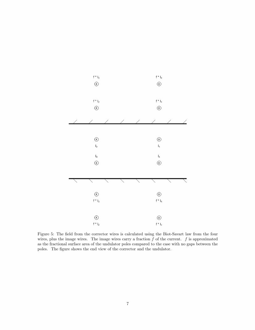
Figure 5: The �eld from the corrector wires is calculated using the Biot-Savart law from the fourwires, plus the image wires. The image wires carry a fraction f of the current. f is approximatedas the fractional surface area of the undulator poles compared to the case with no gaps between thepoles. The �gure shows the end view of the corrector and the undulator.

7

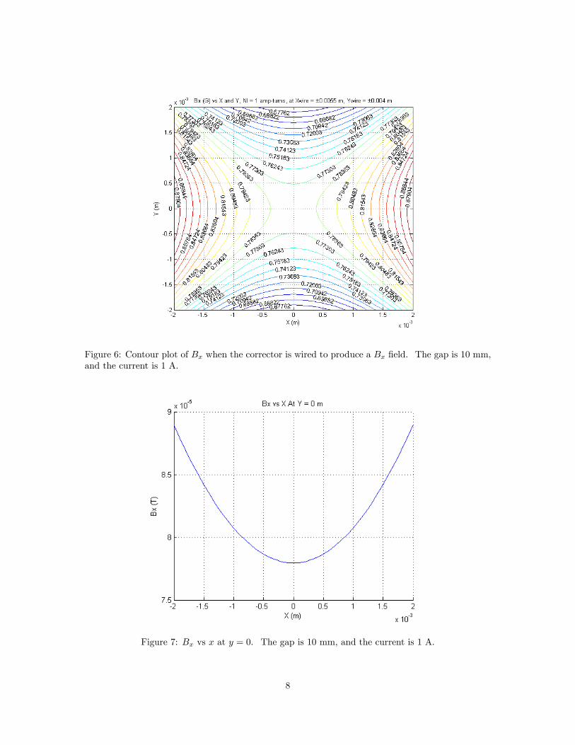
Figure 6: Contour plot of Bx when the corrector is wired to produce a Bx �eld. The gap is 10 mm,and the current is 1 A.

Figure 7: Bx vs x at y = 0. The gap is 10 mm, and the current is 1 A.

8

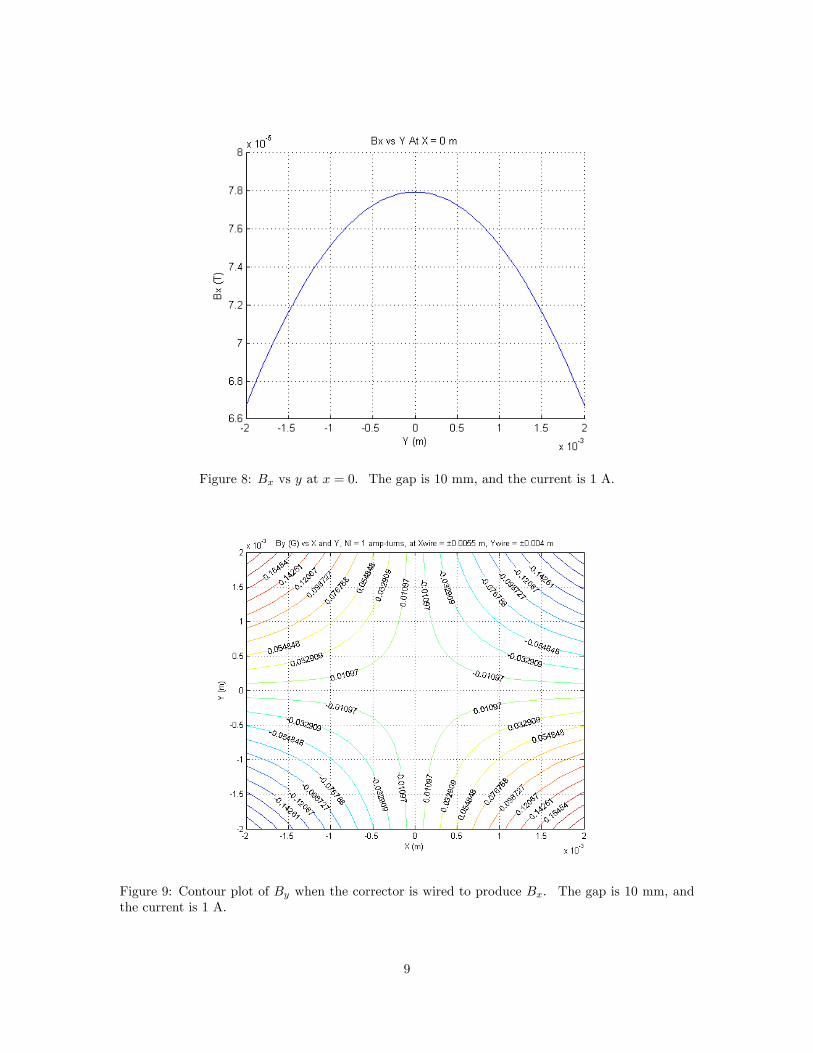
Figure 8: Bx vs y at x = 0. The gap is 10 mm, and the current is 1 A.

Figure 9: Contour plot of By when the corrector is wired to produce Bx. The gap is 10 mm, andthe current is 1 A.

9

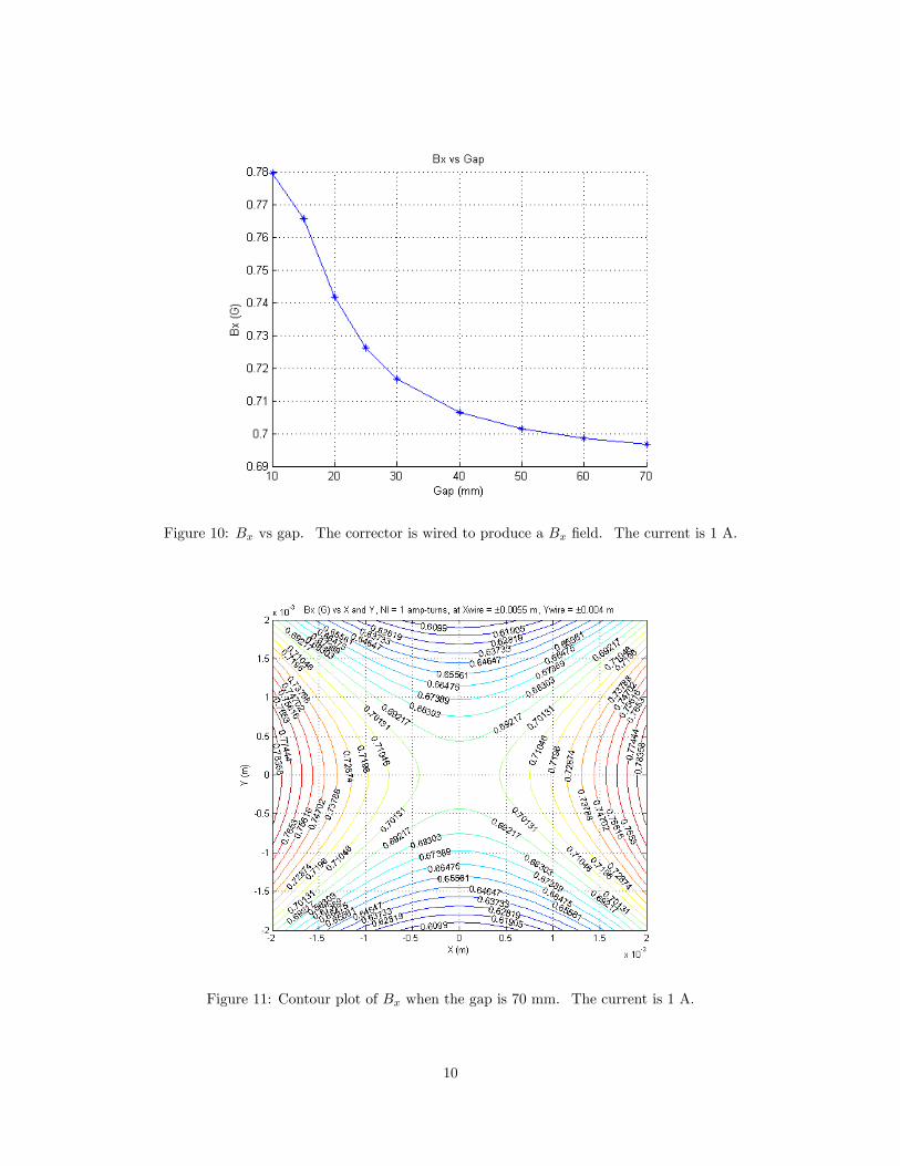
Figure 10: Bx vs gap. The corrector is wired to produce a Bx �eld. The current is 1 A.

Figure 11: Contour plot of Bx when the gap is 70 mm. The current is 1 A.

10

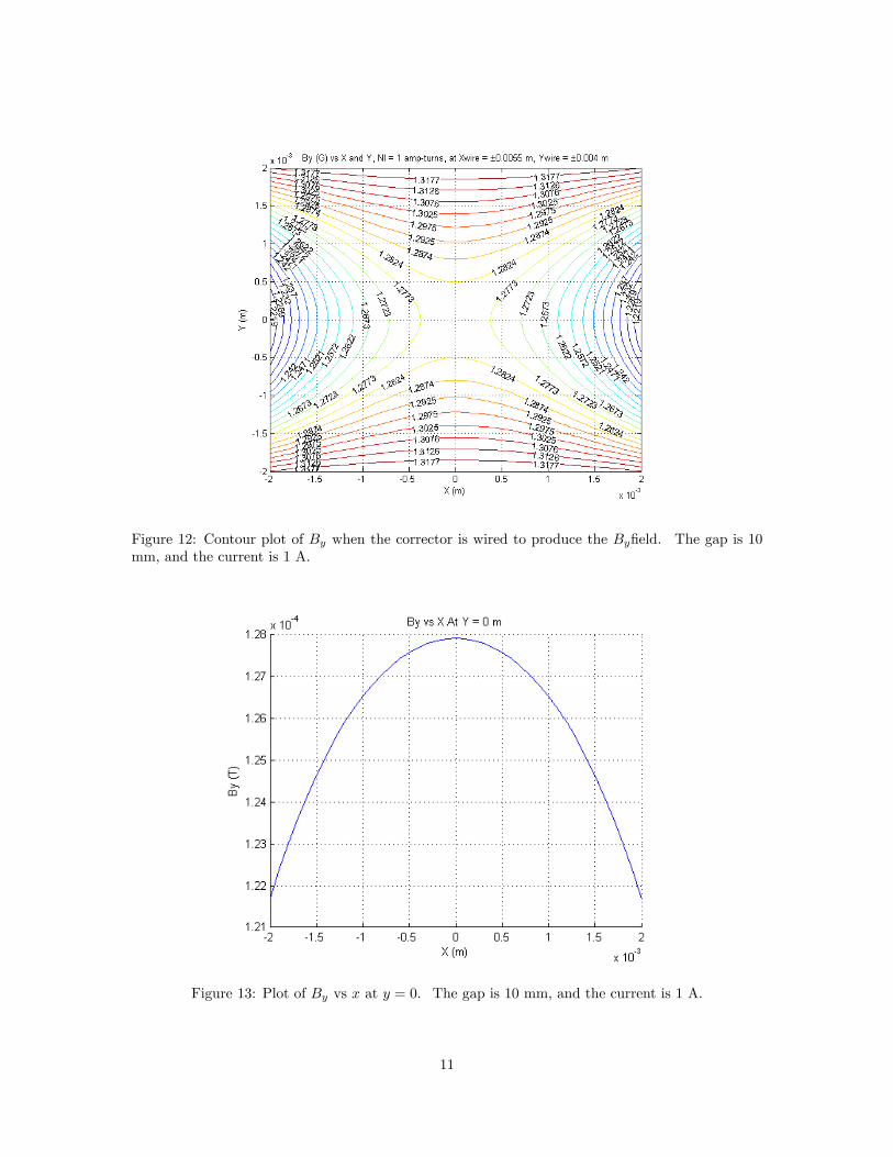
Figure 12: Contour plot of By when the corrector is wired to produce the By�eld. The gap is 10mm, and the current is 1 A.

Figure 13: Plot of By vs x at y = 0. The gap is 10 mm, and the current is 1 A.

11

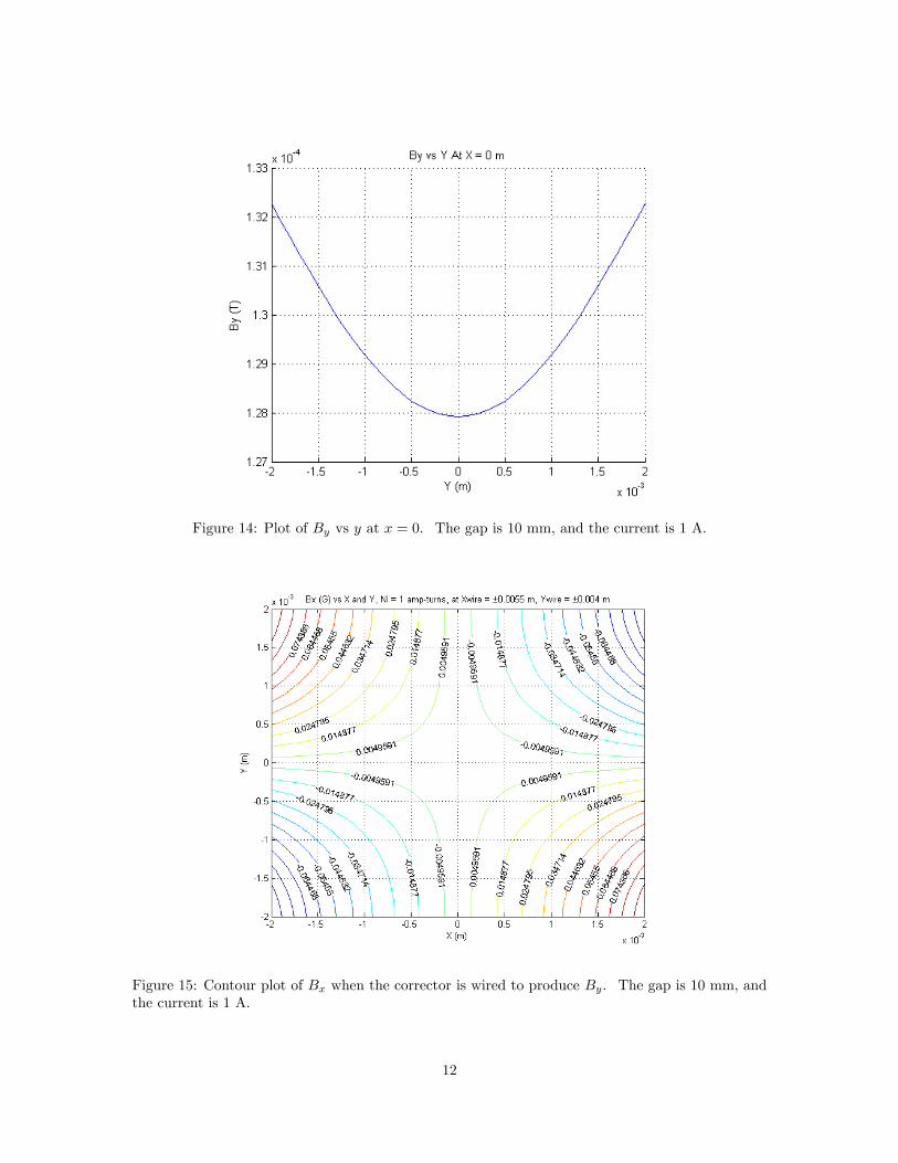
Figure 14: Plot of By vs y at x = 0. The gap is 10 mm, and the current is 1 A.

Figure 15: Contour plot of Bx when the corrector is wired to produce By. The gap is 10 mm, andthe current is 1 A.

12

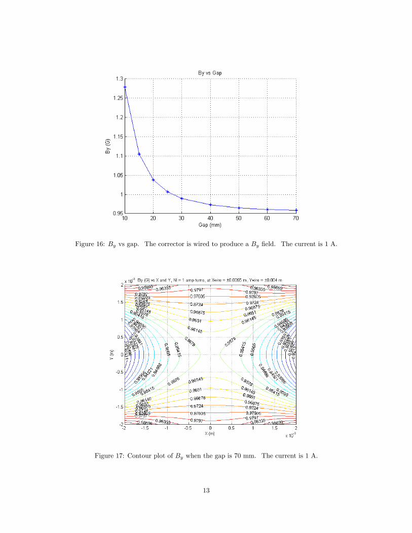
Figure 16: By vs gap. The corrector is wired to produce a By �eld. The current is 1 A.

Figure 17: Contour plot of By when the gap is 70 mm. The current is 1 A.

13

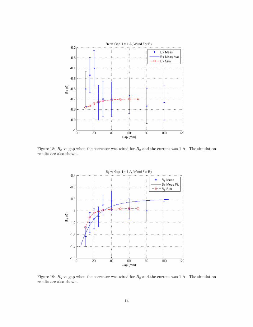
Figure 18: Bx vs gap when the corrector was wired for Bx and the current was 1 A. The simulationresults are also shown.

Figure 19: By vs gap when the corrector was wired for By and the current was 1 A. The simulationresults are also shown.

14

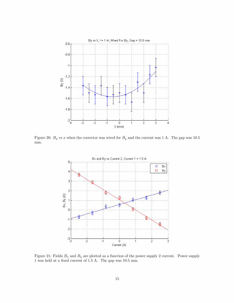
Figure 20: By vs x when the corrector was wired for By and the current was 1 A. The gap was 10:5mm.

Figure 21: Fields Bx and By are plotted as a function of the power supply 2 current. Power supply1 was held at a �xed current of 1:5 A. The gap was 10:5 mm.

15

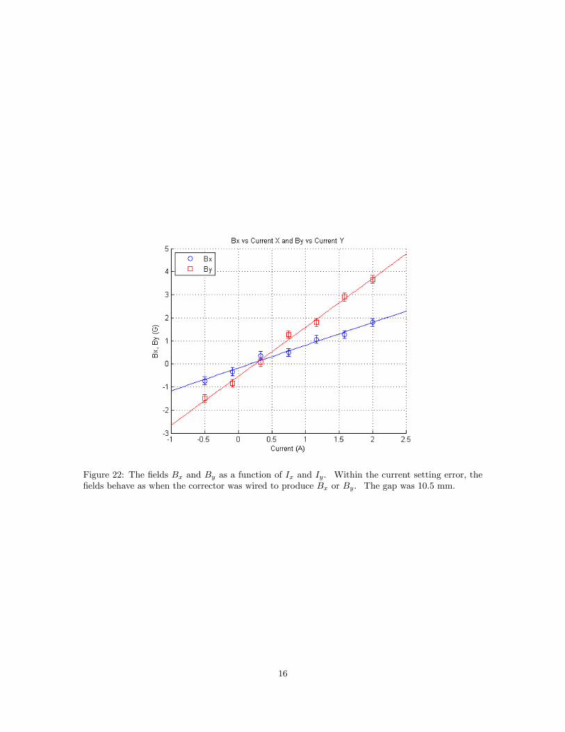
Figure 22: The �elds Bx and By as a function of Ix and Iy. Within the current setting error, the�elds behave as when the corrector was wired to produce Bx or By. The gap was 10:5 mm.

16