Embed Size (px)
Citation preview
Finite Element Method II
Structural elements
3D beam element
1
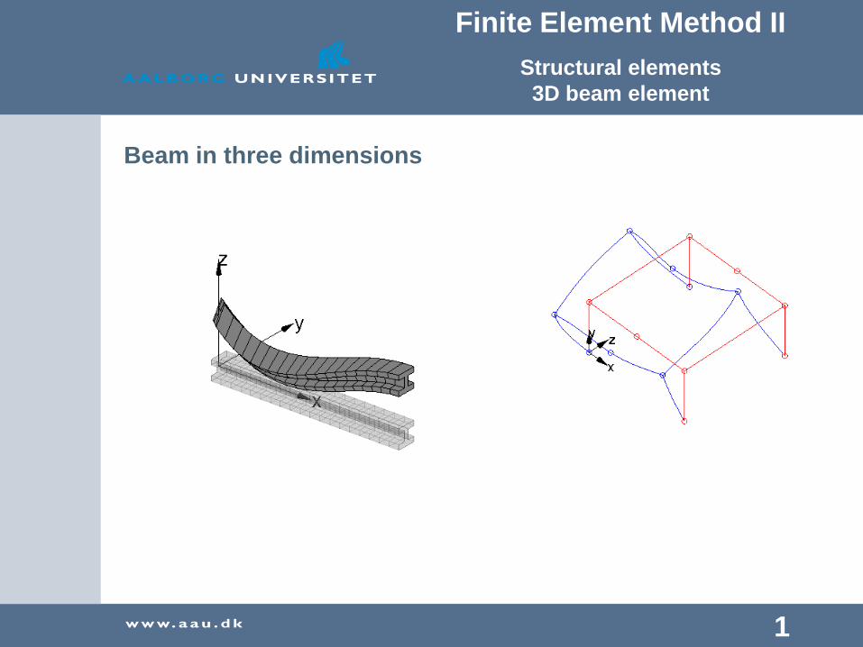
Beam in three dimensions

Finite Element Method II
Structural elements
3D beam element
2
Lecture plan

Finite Element Method II
Structural elements
3D beam element
3
Basic steps of the finite-element method (FEM)
1. Establish strong formulation
Partial differential equation
2. Establish weak formulation
Multiply with arbitrary field and integrate over element
3. Discretize over space
Mesh generation
4. Select shape and weight functions
Galerkin method
5. Compute element stiffness matrix
Local and global system
6. Assemble global system stiffness matrix
7. Apply nodal boundary conditions
temperature/flux/forces/forced displacements
8. Solve global system of equations
Solve for nodal values of the primary variables
(displacements/temperature)
9. Compute temperature/stresses/strains etc. within the element
Using nodal values and shape functions

Finite Element Method II
Structural elements
3D beam element
4
Structural elements, n degrees-of-freedom (ndof) in each
node
degrees-of-freedom are displacement or rotation components in
cartesian coordinate system and these are the so-called primary
variables we solve for
A 3D beam has 6dof in each node:
2 nodes, one at each end (in this case)
3 deformation components
3 rotation components
node 1 node 2
Finite Element Method II
Structural elements
3D beam element
5
Beam assumptions, (Cook: section 2.3-2.5 p24-36),
(OP:chapter 17, p311-334)
Small deformations
axial deformation, bending and twist can be decoupled and looked at
seperately
Bernoulli-Euler beam theory for bending
Plane sections normal to the beam axis remain plane and normal to the
beam axis during the deformation.
Twist is considered free
Saint-Venant torsion
Finite Element Method II
Structural elements
3D beam element
6
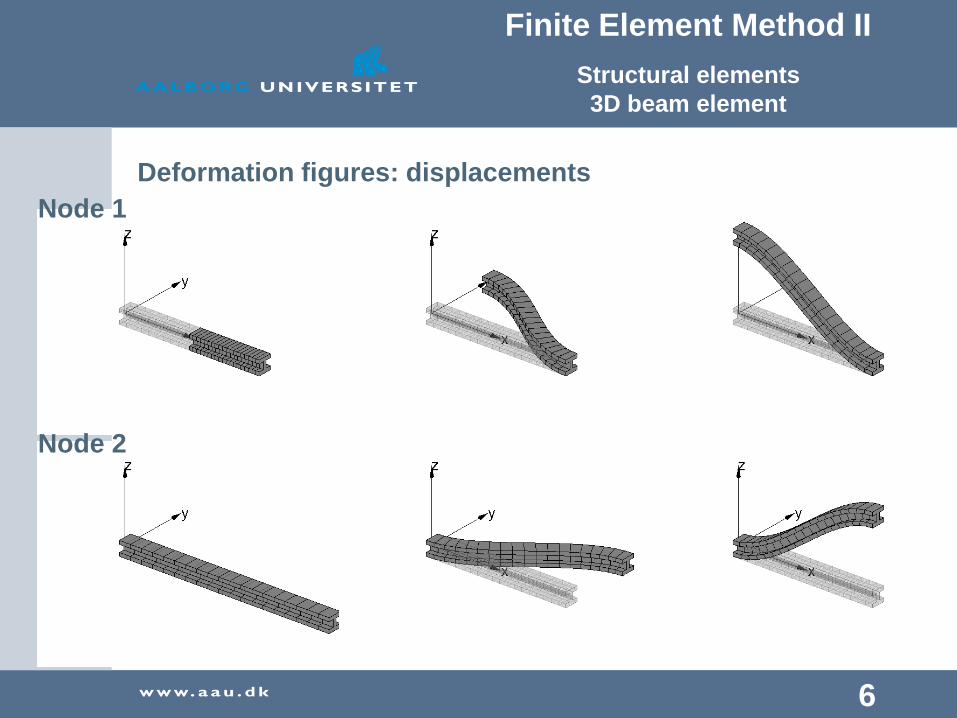
Deformation figures: displacements
Node 1
Node 2

Finite Element Method II
Structural elements
3D beam element
7
Deformation figures: rotations
Node 1
Node 2

Finite Element Method II
Structural elements
3D beam element
8
step 1: Strong formulation for axial deformation, (Cook:
section 2.2 p20-21), (OP: p52-53)

Finite Element Method II
Structural elements
3D beam element
9
equlibrium equation, see slide 20-21 lecture 1
Sum of all forces are equal to zero
The force in terms of normal stress
Material property or constitutive relation (Hooks law)
Kinematic relation or geometric relation
axial deformation equation
¡N + bdx+N + dN = 0 )dN
dx+ b = 0
N =A¾

Finite Element Method II
Structural elements
3D beam element
10
Second order differential equation needs two boundary conditions
Possible boundary conditions: displacement (kinematic) or
displacement gradient (boundary force,static)
This is the strong formulation axial deformation

Finite Element Method II
Structural elements
3D beam element
11
Step 2: Establish weak formulation
Strong form
Multiply with an arbitrary function v(x) (weight function) and integrate
over the pertinent region

Finite Element Method II
Structural elements
3D beam element
12
Use integration by parts of the first term to obtain the same
derivative of the weight function and primary variable u
Weak formulation of axial deformation
boundary conditionsdistributed load

Finite Element Method II
Structural elements
3D beam element
13
Step 3: Discretize over space
Discretized problem. Define: nodes, unknown (degree-of-freedom dof)
numbering, element numbering
Nodes
Elements
dof
coordinateNode number

Finite Element Method II
Structural elements
3D beam element
14
Step 4: Select shape and weight functions (Cook: section
3.2-3.3 p83-91), (OP: chapter 7, 98-106)
Assuming nodal values to be known
Linear variation of deformation allows a constant deformation
gradient (strain)
Simplest one-dimensional element (p98-99)
Matrix notation
shape functions
nodal values (dof)
Finite Element Method II
Structural elements
3D beam element
15
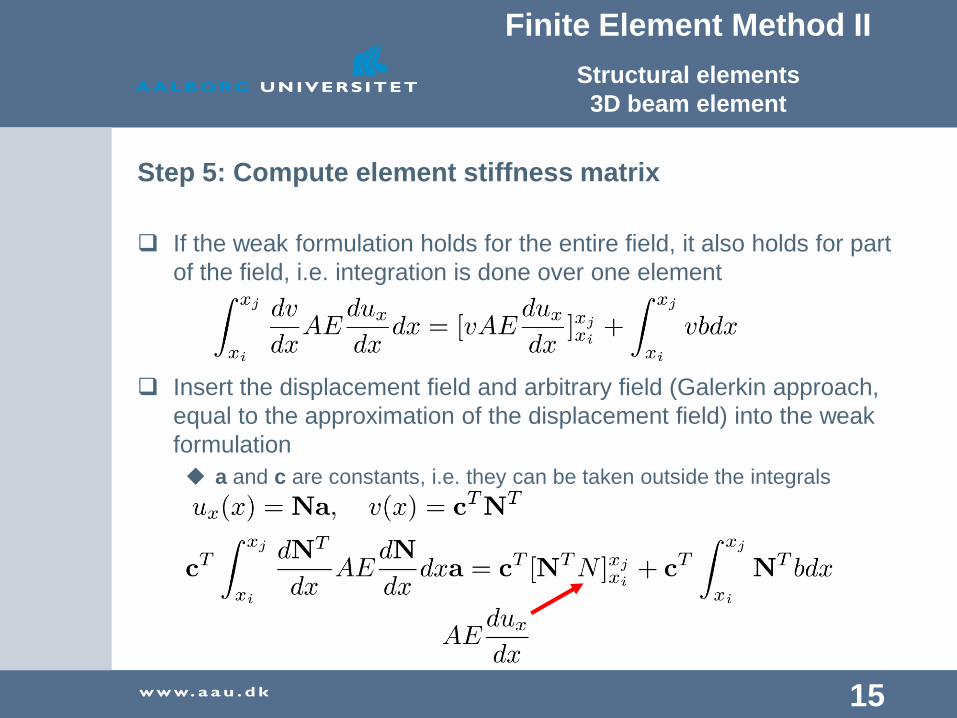
Step 5: Compute element stiffness matrix
If the weak formulation holds for the entire field, it also holds for part
of the field, i.e. integration is done over one element
Insert the displacement field and arbitrary field (Galerkin approach,
equal to the approximation of the displacement field) into the weak
formulation
a and c are constants, i.e. they can be taken outside the integrals

Finite Element Method II
Structural elements
3D beam element
16
In compact form

Finite Element Method II
Structural elements
3D beam element
17
Exercise: Determine the stiffness matrix for the axial
deformation
Solve the integral on slide 17
Enter the stiffness matrix into the local stiffness matrix in
K_3d_beam.m
The local element dof are u1 and u7, i.e. the stiffness should be added to
rows and columns 1 and 7. This is easily done by the following way Kel([1 7],[1 7]) = [ - - ; - - ]

Finite Element Method II
Structural elements
3D beam element
18
Exercise: Enter the shape functions in shape_3d_beam.m
Enter N1 and N2 from slide 17 into the function
Test the shape function in the program beam_shape_test.m
Try to run the program with different displacements
u1=1 u7=1

Finite Element Method II
Structural elements
3D beam element
19
Beam bending problem in the xz-plane, (Cook: section 2.3
p24-27), (OP: chapter 17, p 311-334)
u3=1 u5=1 u9=1 u11=1

Finite Element Method II
Structural elements
3D beam element
20
step 1: strong formulation, (OP: p.311-318)
Infinitely small part of the beam
Vertical equilibrium
Moment equilibrium around left end, counter clockwise
second order terms are disregarded
Finite Element Method II
Structural elements
3D beam element
21
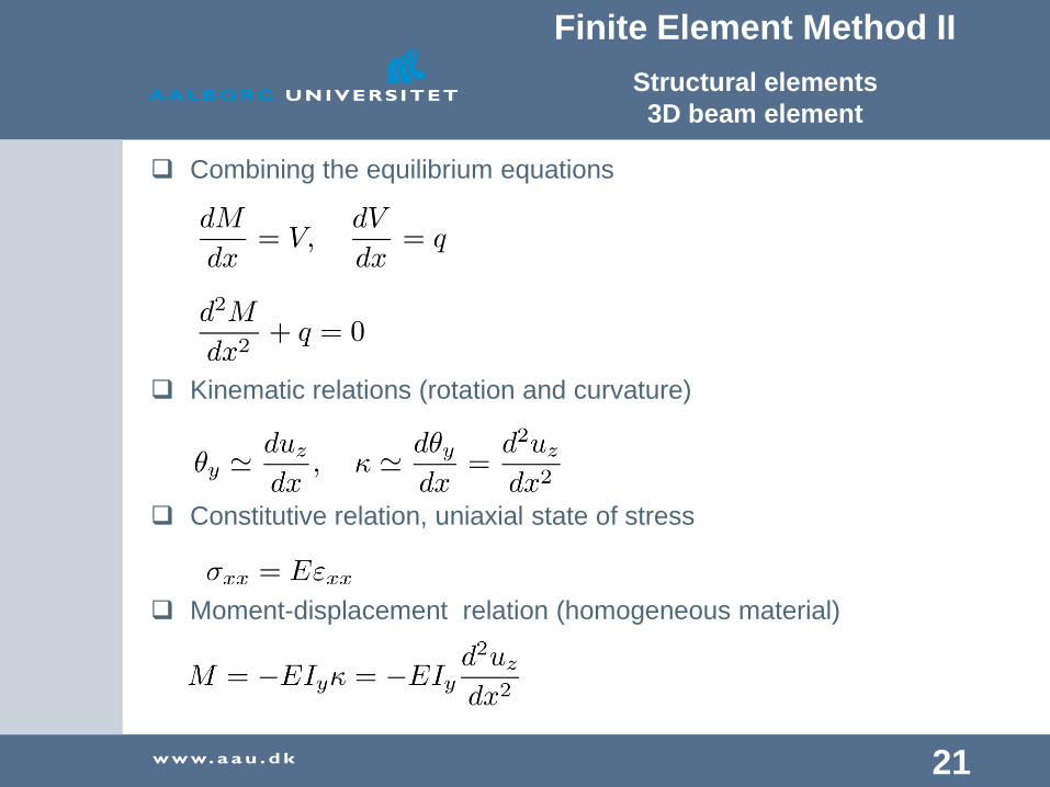
Combining the equilibrium equations
Kinematic relations (rotation and curvature)
Constitutive relation, uniaxial state of stress
Moment-displacement relation (homogeneous material)

Finite Element Method II
Structural elements
3D beam element
22
Strong formulation in terms of displacements
4th order differential equation, 4 boundary conditions (two at each
end)
Free end
Simple support
Fixed support

Finite Element Method II
Structural elements
3D beam element
23
Assumptions in the formulation, (Cook: p28-29),
(OP: p315-317)
rotation is taken as first derivative of displacement. This is only
approximately true if the displacements are small
The shear strain is assumed equal to zeros which gives zeros shear
stress. This is not true but comes out of simplifying a 3D problem to
2D. We will not be concerned about this inconsistency
The beam axis is located at the so-called neutral axis where an
evenly distribution of normal stresses don't introduce a moment.
This gives that the axial and bending problem decouples and can be
considered separately.

Finite Element Method II
Structural elements
3D beam element
24
step 2: weak formulation, (OP: p.318-319)
Multiply with arbitrary field and integrate over element
Integrate by parts

Finite Element Method II
Structural elements
3D beam element
25
Integrate by parts again
boundary conditionsdistributed load

Finite Element Method II
Structural elements
3D beam element
26
Step 3: Discretize over space
Discretized problem. Define: nodes, unknown (degree-of-freedom dof)
numbering, element numbering

Finite Element Method II
Structural elements
3D beam element
27
Step 4: Select shape and weight functions,
(Cook: sektion 3.2-3.3 p83-91), (OP: p.323-328)
Assuming nodal values to be known
The approximation for the deflection must be able to produce a
constant deflection and curvature, i.e. it should at least be twice
differentiable.
The second derivative of the displacements enters the formulation
hence the first derivative should be continuous over element
boundaries (C1-continuity) , or the second derivative will be infinite.
We have four node values available, i.e. four shape functions giving
the deformation shape
C0 continuity C1 continuity

Finite Element Method II
Structural elements
3D beam element
28
Shape functions
test u3=1, u5=u9=u11=0

Finite Element Method II
Structural elements
3D beam element
29

Finite Element Method II
Structural elements
3D beam element
30
Including all dof

Finite Element Method II
Structural elements
3D beam element
31
Exercise: Enter the shape functions in shape_3d_beam.m
Enter N3 - N6 from slide 28-29 into the function
Test the shape function in the program beam3D_example.m, make
sure the signs are correct!
Try to run the program with different displacements
u3=1 u11=1

Finite Element Method II
Structural elements
3D beam element
32
step 5: compute the element stiffness matrix
Weak form
FE approximation

Finite Element Method II
Structural elements
3D beam element
33
In compact form
natural boundary
conditions, cancels
between elements.
Only at supports they
have a value
(reactions).
consistent load

Finite Element Method II
Structural elements
3D beam element
34
Exercise: solve the bending in the xz-plane part of the
stiffness matrix and enter into K_3d_beam.m
The local element dof are u3, u5, u9 and u11, i.e. the stiffness should be added
to rows and columns 3, 5, 9 and 11. This is easily done by
Kel([3 5 9 11],[3 5 9 11]) =

Finite Element Method II
Structural elements
3D beam element
35
xy-plane, what changes? (Cook: p27-28)
index for dof
Signs on shape functions for rotation
u6=1 u5=1 u12=1 u11=1
Finite Element Method II
Structural elements
3D beam element
36
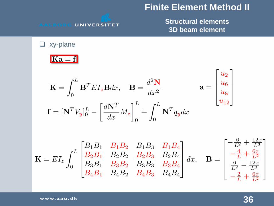
xy-plane
Finite Element Method II
Structural elements
3D beam element
37
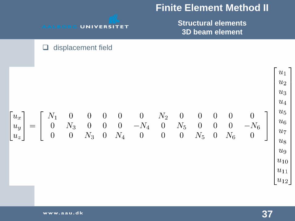
displacement field

Finite Element Method II
Structural elements
3D beam element
38
Free Torsion, Saint-Venant, (Cook: p27-28), (OP: chapter 14,
p261-281)
u4=1 u10=1

Finite Element Method II
Structural elements
3D beam element
39
Torsional stiffness

Finite Element Method II
Structural elements
3D beam element
40
Torsional moment of inertia
Thin walled sections (statik 4, 5th semester, 4th lecture)
Open sections Closed sections (Bredts equation)
"Teknisk STÅBI", steel sections
From bending moment of inertia

Finite Element Method II
Structural elements
3D beam element
41
FE formulation is identical with the axial deformation
See slide 9
Torsion
mx is a distributed twisting load
A linear approximation (shape function) for the torsion between the
nodes, see slide 14
Finite Element Method II
Structural elements
3D beam element
42
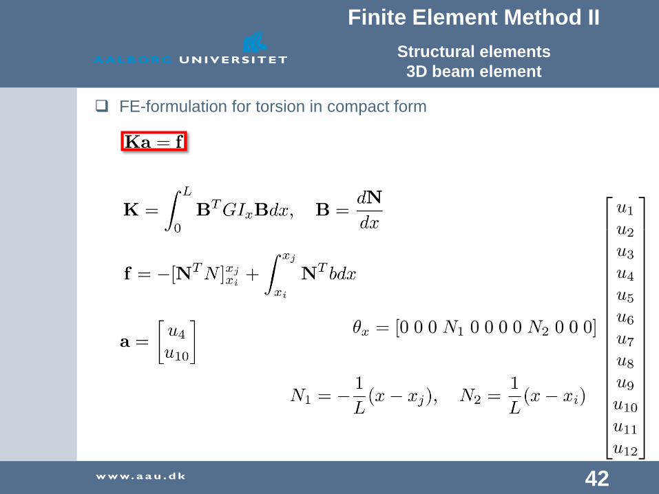
FE-formulation for torsion in compact form

Finite Element Method II
Structural elements
3D beam element
43
The full displacement field for a 3D beam

Finite Element Method II
Structural elements
3D beam element
44
Stiffness matrix for torsion is identical with the one for axial
deformation with AE replaced with GIx , se exercise slide 8
The dofs are u4 and u10 , i.e. the stiffness matrix should enter the
corresponding rows and columns

Finite Element Method II
Structural elements
3D beam element
45
Exercise: Type in the stiffness matrix and shape functions and test
your beam element (Teknisk STÅBI)

Finite Element Method II
Structural elements
3D beam element
46
Transformation, (Cook: section 2.4 p29-32)
Why do we need to do a transformation?

Finite Element Method II
Structural elements
3D beam element
47
Local beam axis
Finite Element Method II
Structural elements
3D beam element
48
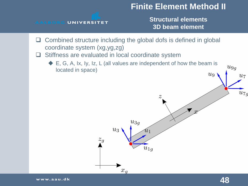
Combined structure including the global dofs is defined in global
coordinate system (xg,yg,zg)
Stiffness are evaluated in local coordinate system
E, G, A, Ix, Iy, Iz, L (all values are independent of how the beam is
located in space)

Finite Element Method II
Structural elements
3D beam element
49
Assume at first that there exists a relation between a vector in the
global coordinate system and local coordinate system (at first we
only consider the xz-plane)
This relation is valid for any vector, e.g. displacement, rotation, force
or moment vector.
transformation matrix

Finite Element Method II
Structural elements
3D beam element
50
Until now everything has been described in a local coordinate
system where the beam axis is located at the local x-axis. I.e. the
element stiffness matrix Ke is described in a local system and the
compact form (slide 16, 33 and 42) is only valid in a local system
a includes both displacements and rotations and f includes both
forces and moments
Property of a transformation matrix T
The global form of the system
Global element stiffness matrix,
this is used to assemble the
global system of equations

Finite Element Method II
Structural elements
3D beam element
51
We have already identified the local element stiffness matrix Ke, all
we need is to determine the transformation matrix T
If we want to describe the components of a vector given in one
coordinate system (xg,yg) in another coordinate system (x,y), we can
multiply the vector with the unit vectors spanning the (x,y) system
This corresponds to rotating the vector - equal the angle between
the two systems

Finite Element Method II
Structural elements
3D beam element
52
Vectors defined in global system
V defined in local system
The transformation matrix is an orthogonal set of unit vectors placed
in the columns. This also holds in 3D

Finite Element Method II
Structural elements
3D beam element
53
In the beam case we need the y- and z-coordinates equal zero (the
beam axis is equal the x-axis). The y- and z-axis are the axis around
which the moments of inertia, Iy and Iz, are defined.
the plane spanned by node 1, node 2 and node 3 defines the xy-
plane
the xz-plane is orthogonal to the xy-plane
I.e. the beam has two nodes but we need three nodes to define the
location in space (this is the only thing the 3rd node is used for)

Finite Element Method II
Structural elements
3D beam element
54
How do we find the unit vectors describing the xyz-system?

Finite Element Method II
Structural elements
3D beam element
55
Exercise: Include the transformation in the program
Update transformation.m according to the previous slide.
Make the full transformation matrix (12x12) from T (3x3) in
K_3d_beam.m and multiply the local element stiffness matrix with
the transformation to obtain the global element stiffness matrix
hint introduce a matrix null = zeros(3,3)
The cross product V3xV1 in matlab: cross(V3,V1);
The transposed: Tg'

Finite Element Method II
Structural elements
3D beam element
56
Test the transformation function
The local y- and z-components should all be zero

Finite Element Method II
Structural elements
3D beam element
57
Exersice: Solve the test case from "Teknisk STÅBI"
supports are type 1 boundary conditions
loads are type 2 boundary conditions
where a type 1 BC has been defined a reaction is determined
where a type 2 BC has been defined a displacement is determined
A BC should be defined in all nodes in all dofs. Where nothing is
defined a load equal 0 is assumed
Below infinite axial stiffness is assumed. How do we get that?

Finite Element Method II
Structural elements
3D beam element
58
Field values: displacement, strain, stress, section forces
All field values are evaluated in local coordinate system, i.e. nodal
dofs needs to be rotated via the transformation matrix [12x12]
We need to identify the numbers of the12 dofs for the beam of interest
done in the matrix ElemDof defined in calc_globdof.m
Normal force, slide 9
Bending moments, slide 22 (index just change when considering Mz
and Vz)
Torsional moment, slide 39
N = EA@ux
@x

Finite Element Method II
Structural elements
3D beam element
59
Derivative of the field values are taken as derivative of the shape
functions multiplied by the nodal values, se slide 43 (used in the
visualization part)

Finite Element Method II
Structural elements
3D beam element
60
Exercise: 3Dframe
Create the indicated geometry

Finite Element Method II
Structural elements
3D beam element
61
Exercise: Varying section height
Divide the beam into 5 elements with varying height

Finite Element Method II
Structural elements
3D beam element
62
Thank you for your attention


![Introduction to Mathematica [p24]](https://img.pdfslide.us/doc/110x75/577cc0de1a28aba71191676b/introduction-to-mathematica-p24.jpg)