Multi-Armed Bandits:Bayesian vs. Frequentist Lorenzo Maggi

Nokia Bell Labs

Basic scenario

• 𝐾 “arms”

• Arm 𝑎 = r.v. with distribution 𝜈𝑎 and mean 𝜇𝑎• 𝜈𝑎 and 𝜇𝑎 are unknown

• test the arms by obtaining i.i.d. samples ∼ 𝜈𝑎 , ∀𝑎

• goal: maximize the sum of rewards (quickly identify 𝑎∗ = argmax𝑎 𝜇𝑎)

Exploration/exploitation dilemma• 𝐾 “arms”

• Arm 𝑎 = r.v. with distribution 𝜈𝑎 and mean 𝜇𝑎

• 𝜈𝑎 and 𝜇𝑎 are unknown

• goal: maximize the sum of rewards (𝑎∗ = argmax𝑎 𝜇𝑎)

• How? “test” the arms by obtaining i.i.d. samples ∼ 𝜈𝑎, ∀𝑎

• At time 𝑡 we have sampled arms and built estimates ො𝜇𝑎,𝑡 ≈ 𝜇𝑎, ∀𝑎

• Dilemma:• (exploitation) settle for our current estimates and greedily choose what

seems to be the best arm ( ො𝑎𝑡 = argmax𝑎 Ƹ𝜇𝑎,𝑡)

• (exploration) keep sampling the “bad” arms to make sure they’re really bad

explore… Exploit!

A simple example

• Arm 1: fixed reward 𝑌1,𝑡= 0.25 𝜈1 = 𝛿0.25, 𝜇1 = 0.25

• Arm 2: 𝑌2,𝑡 =ቊ0 𝑤. 𝑝. 0.31 𝑤. 𝑝. 0.7

→ 𝜇2= 0.7

• Oracle policy: always pick arm 2 unbeatable but not implementable

• Greedy policy: choose the arm with highest estimated avg. reward with probability 0.3, we choose the bad arm forever! (linear regret)• (exploration) time 1: arm 1, reward 0.25 ො𝜇1 = .25• (exploration) time 2: arm 2, reward 0 w.p. 0.3 ො𝜇2 = 0• (exploitation) time 3: greedily choose arm 1 ො𝜇1 = .25• (exploitation) time 3: greedily choose arm 1 ො𝜇1 = .25• … forever and ever…

• What else…?

Applications

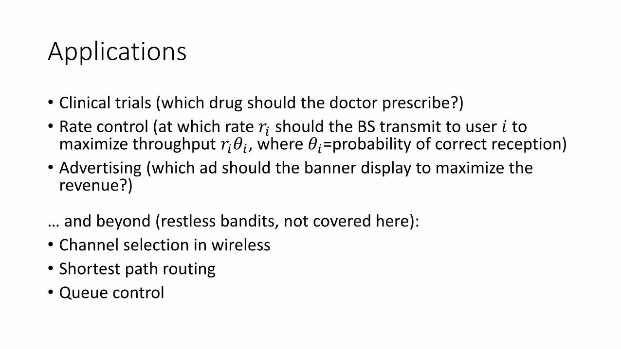
• Clinical trials (which drug should the doctor prescribe?)

• Rate control (at which rate 𝑟𝑖 should the BS transmit to user 𝑖 to maximize throughput 𝑟𝑖𝜃𝑖, where 𝜃𝑖=probability of correct reception)

• Advertising (which ad should the banner display to maximize the revenue?)

… and beyond (restless bandits, not covered here):

• Channel selection in wireless

• Shortest path routing

• Queue control

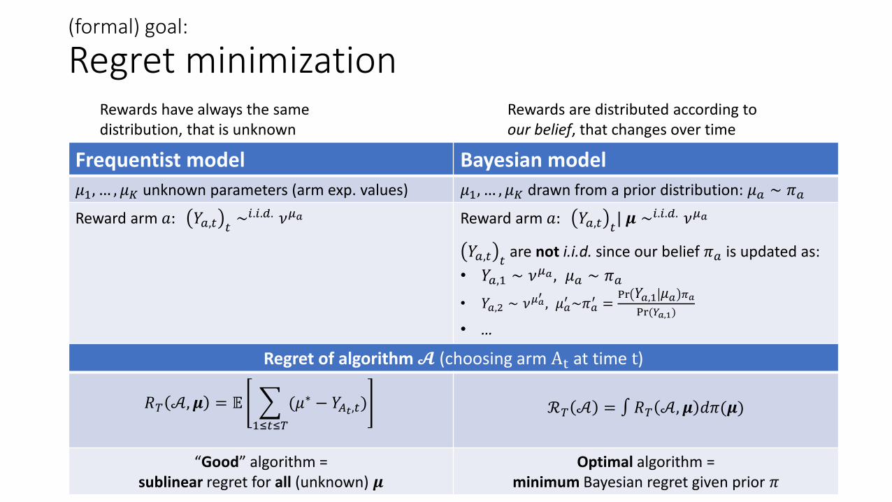
(formal) goal:

Regret minimization

Frequentist model Bayesian model

𝜇1, … , 𝜇𝐾 unknown parameters (arm exp. values) 𝜇1, … , 𝜇𝐾 drawn from a prior distribution: 𝜇𝑎 ∼ 𝜋𝑎

Reward arm 𝑎: 𝑌𝑎,𝑡 𝑡∼𝑖.𝑖.𝑑. 𝜈𝜇𝑎 Reward arm 𝑎: 𝑌𝑎,𝑡 𝑡

| 𝝁 ∼𝑖.𝑖.𝑑. 𝜈𝜇𝑎

𝑌𝑎,𝑡 𝑡are not i.i.d. since our belief 𝜋𝑎 is updated as:

• 𝑌𝑎,1 ∼ 𝜈𝜇𝑎 , 𝜇𝑎 ∼ 𝜋𝑎

• 𝑌𝑎,2 ∼ 𝜈𝜇𝑎′, 𝜇𝑎

′ ~𝜋𝑎′ =

Pr 𝑌𝑎,1 𝜇𝑎 𝜋𝑎

Pr(𝑌𝑎,1)

• …

Rewards are distributed according to our belief, that changes over time

Rewards have always the same distribution, that is unknown

Regret of algorithm 𝓐 (choosing arm At at time t)

𝑅𝑇 𝒜,𝝁 = 𝔼

1≤𝑡≤𝑇

(𝜇∗ − 𝑌𝐴𝑡,𝑡) ℛ𝑇 𝒜 = ∫𝑅𝑇 𝒜,𝝁 𝑑𝜋(𝝁)

“Good” algorithm = sublinear regret for all (unknown) 𝝁

Optimal algorithm = minimum Bayesian regret given prior 𝜋

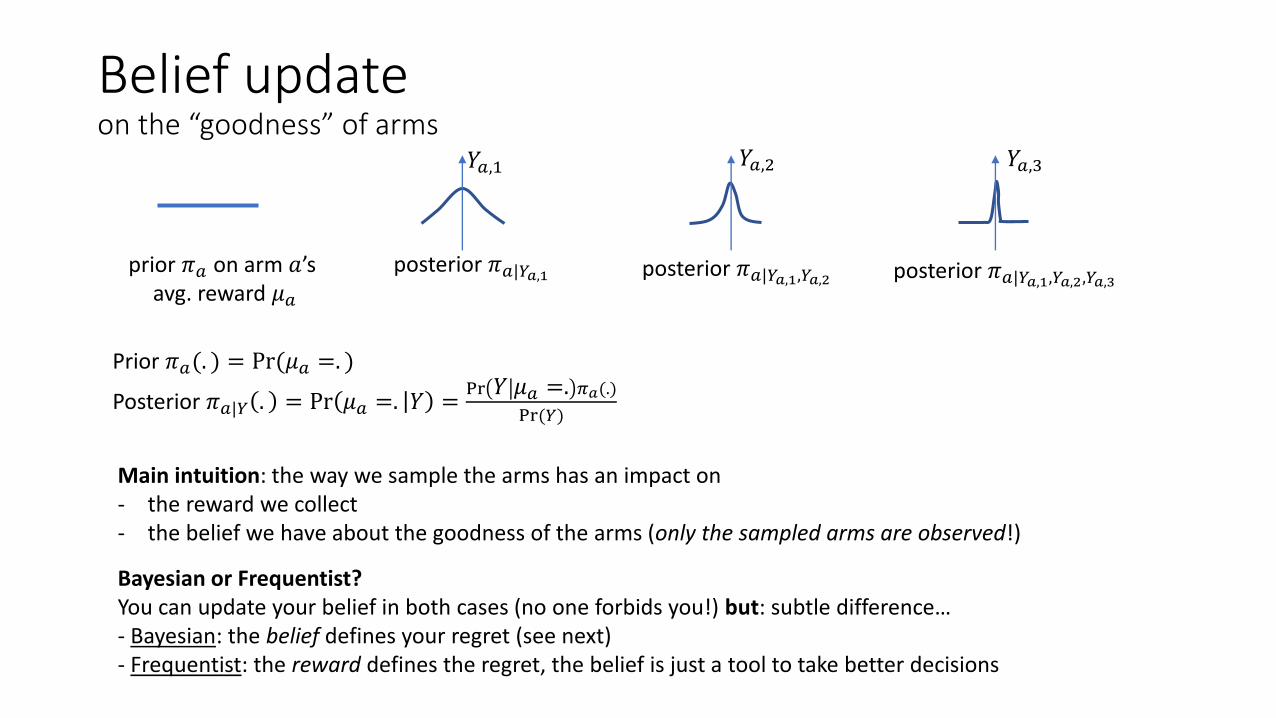
Belief update on the “goodness” of arms

prior 𝜋𝑎 on arm 𝑎’s avg. reward 𝜇𝑎

posterior 𝜋𝑎|𝑌𝑎,1 posterior 𝜋𝑎|𝑌𝑎,1,𝑌𝑎,2 posterior 𝜋𝑎|𝑌𝑎,1,𝑌𝑎,2,𝑌𝑎,3

𝑌𝑎,1 𝑌𝑎,2 𝑌𝑎,3

Prior 𝜋𝑎(. ) = Pr(𝜇𝑎 =. )

Posterior 𝜋𝑎|𝑌 . = Pr 𝜇𝑎 =. 𝑌 =Pr 𝑌 𝜇𝑎 =. 𝜋𝑎(.)

Pr(𝑌)

Main intuition: the way we sample the arms has an impact on- the reward we collect- the belief we have about the goodness of the arms (only the sampled arms are observed!)

Bayesian or Frequentist? You can update your belief in both cases (no one forbids you!) but: subtle difference…- Bayesian: the belief defines your regret (see next)- Frequentist: the reward defines the regret, the belief is just a tool to take better decisions

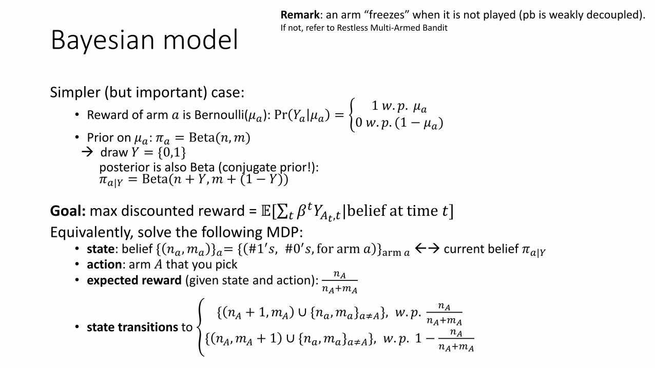
Bayesian model

Bayesian model

Simpler (but important) case:

• Reward of arm 𝑎 is Bernoulli(𝜇𝑎): Pr 𝑌𝑎 𝜇𝑎 = ቊ1 𝑤. 𝑝. 𝜇𝑎

0 𝑤. 𝑝. (1 − 𝜇𝑎)• Prior on 𝜇𝑎: 𝜋𝑎 = Beta(𝑛,𝑚) draw 𝑌 = {0,1}

posterior is also Beta (conjugate prior!): 𝜋𝑎|𝑌 = Beta(𝑛 + 𝑌,𝑚 + (1 − 𝑌))

Goal: max discounted reward = 𝔼[σ𝑡 𝛽𝑡𝑌𝐴𝑡,𝑡|belief at time 𝑡]

Equivalently, solve the following MDP:• state: belief { 𝑛𝑎, 𝑚𝑎 }𝑎= { #1′𝑠, #0′𝑠, for arm 𝑎 }arm 𝑎 current belief 𝜋𝑎|𝑌• action: arm 𝐴 that you pick• expected reward (given state and action):

𝑛𝐴

𝑛𝐴+𝑚𝐴

• state transitions to ൞{ 𝑛𝐴 + 1,𝑚𝐴 ∪ {𝑛𝑎, 𝑚𝑎}𝑎≠𝐴}, 𝑤. 𝑝.

𝑛𝐴

𝑛𝐴+𝑚𝐴

{ 𝑛𝐴, 𝑚𝐴 + 1 ∪ {𝑛𝑎, 𝑚𝑎}𝑎≠𝐴}, 𝑤. 𝑝. 1 −𝑛𝐴

𝑛𝐴+𝑚𝐴

Remark: an arm “freezes” when it is not played (pb is weakly decoupled).If not, refer to Restless Multi-Armed Bandit

Index policy

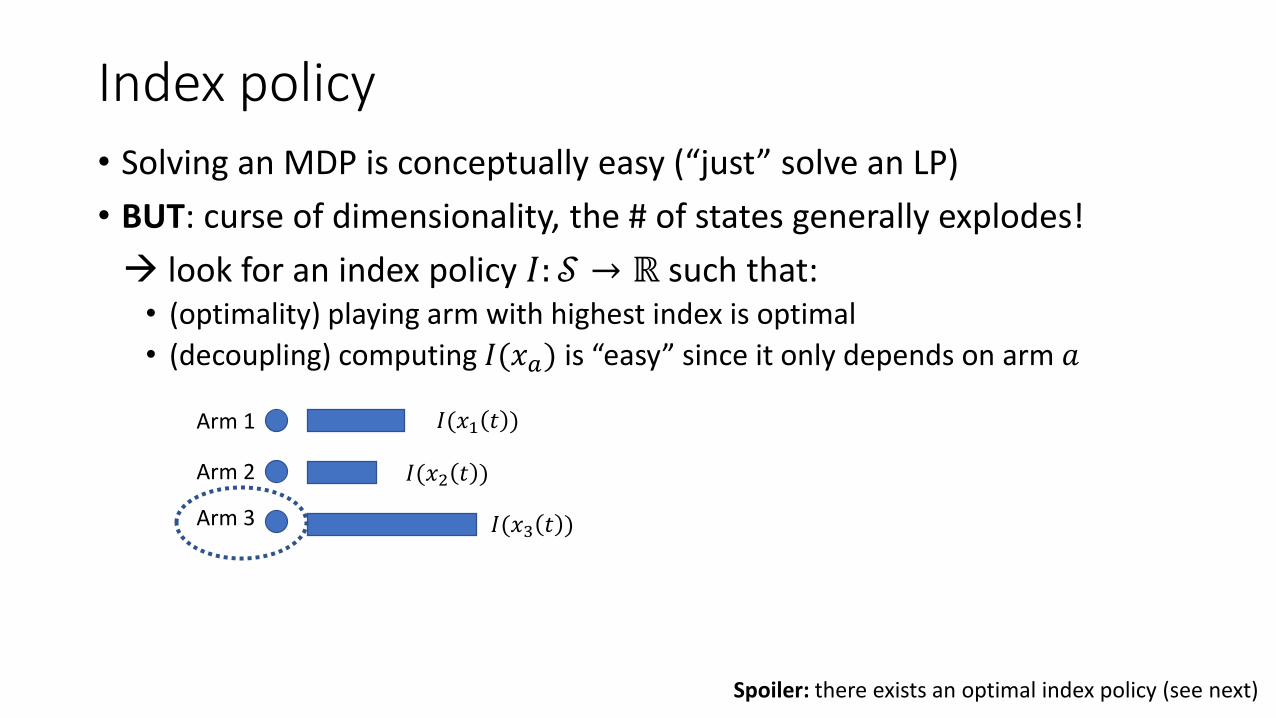
• Solving an MDP is conceptually easy (“just” solve an LP)

• BUT: curse of dimensionality, the # of states generally explodes!

look for an index policy 𝐼: 𝒮 → ℝ such that:• (optimality) playing arm with highest index is optimal

• (decoupling) computing 𝐼(𝑥𝑎) is “easy” since it only depends on arm 𝑎

𝐼(𝑥1 𝑡 )Arm 1

Arm 2

Arm 3

𝐼(𝑥2 𝑡 )

𝐼(𝑥3 𝑡 )

Spoiler: there exists an optimal index policy (see next)

Let’s prove the optimality of Gittins index

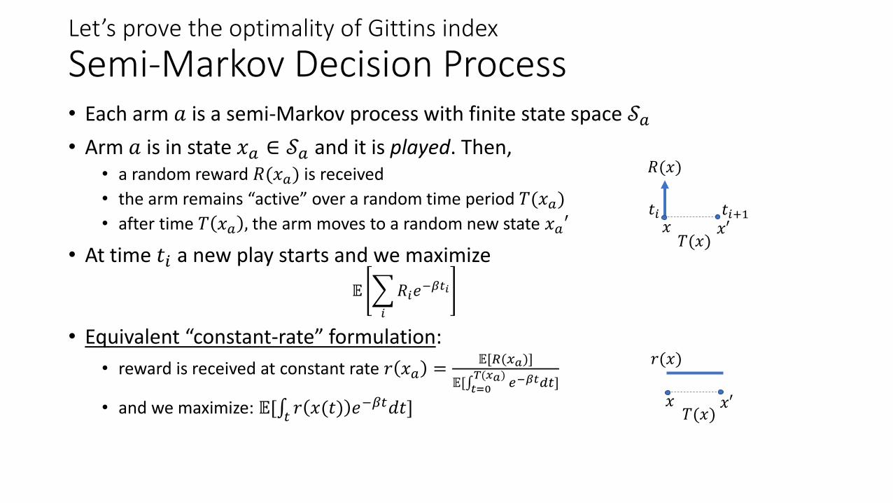
Semi-Markov Decision Process• Each arm 𝑎 is a semi-Markov process with finite state space 𝒮𝑎

• Arm 𝑎 is in state 𝑥𝑎 ∈ 𝒮𝑎 and it is played. Then,• a random reward 𝑅(𝑥𝑎) is received

• the arm remains “active” over a random time period 𝑇(𝑥𝑎)

• after time 𝑇 𝑥𝑎 , the arm moves to a random new state 𝑥𝑎′

• At time 𝑡𝑖 a new play starts and we maximize

𝔼

𝑖

𝑅𝑖𝑒−𝛽𝑡𝑖

• Equivalent “constant-rate” formulation:

• reward is received at constant rate 𝑟 𝑥𝑎 =𝔼[𝑅(𝑥𝑎)]

𝔼[∫𝑡=0𝑇(𝑥𝑎) 𝑒−𝛽𝑡𝑑𝑡]

• and we maximize: 𝔼[∫𝑡 𝑟 𝑥(𝑡) 𝑒−𝛽𝑡𝑑𝑡]

𝑅(𝑥)

𝑇(𝑥)𝑥′𝑥

𝑟(𝑥)

𝑇(𝑥)𝑥′𝑥

𝑡𝑖 𝑡𝑖+1

Gittins index policy

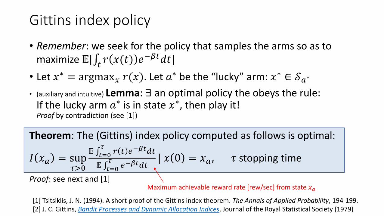
• Remember: we seek for the policy that samples the arms so as to maximize 𝔼[∫𝑡 𝑟 𝑥(𝑡) 𝑒−𝛽𝑡𝑑𝑡]

• Let 𝑥∗ = argmax𝑥 𝑟(𝑥). Let 𝑎∗ be the “lucky” arm: 𝑥∗ ∈ 𝒮𝑎∗

• (auxiliary and intuitive) Lemma: ∃ an optimal policy the obeys the rule:If the lucky arm 𝑎∗ is in state 𝑥∗, then play it!Proof by contradiction (see [1])

Theorem: The (Gittins) index policy computed as follows is optimal:

𝐼 𝑥𝑎 = sup𝜏>0

𝔼 ∫𝑡=0𝜏

𝑟 𝑡 𝑒−𝛽𝑡𝑑𝑡

𝔼 ∫𝑡=0𝜏

𝑒−𝛽𝑡𝑑𝑡| 𝑥 0 = 𝑥𝑎, 𝜏 stopping time

Proof: see next and [1]

[1] Tsitsiklis, J. N. (1994). A short proof of the Gittins index theorem. The Annals of Applied Probability, 194-199.[2] J. C. Gittins, Bandit Processes and Dynamic Allocation Indices, Journal of the Royal Statistical Society (1979)

Maximum achievable reward rate [rew/sec] from state 𝑥𝑎

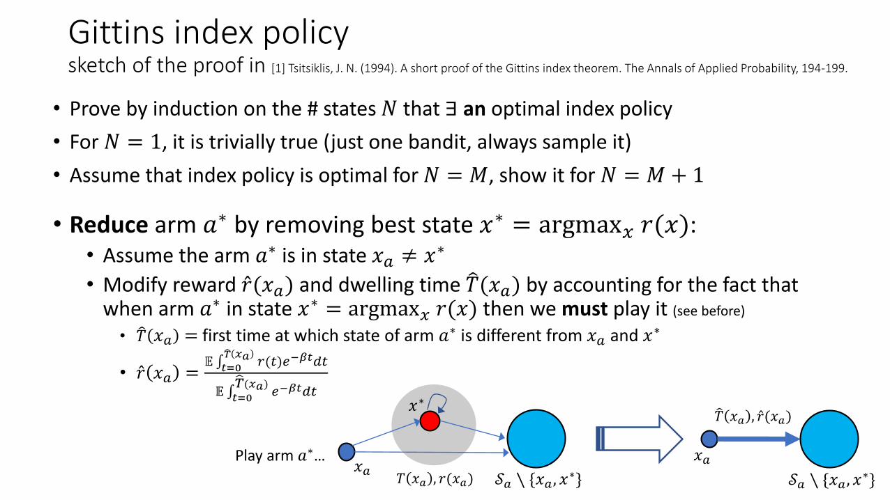
Gittins index policysketch of the proof in [1] Tsitsiklis, J. N. (1994). A short proof of the Gittins index theorem. The Annals of Applied Probability, 194-199.

• Prove by induction on the # states 𝑁 that ∃ an optimal index policy

• For 𝑁 = 1, it is trivially true (just one bandit, always sample it)

• Assume that index policy is optimal for 𝑁 = 𝑀, show it for 𝑁 = 𝑀 + 1

• Reduce arm 𝑎∗ by removing best state 𝑥∗ = argmax𝑥 𝑟(𝑥):• Assume the arm 𝑎∗ is in state 𝑥𝑎 ≠ 𝑥∗

• Modify reward Ƹ𝑟(𝑥𝑎) and dwelling time 𝑇(𝑥𝑎) by accounting for the fact that when arm 𝑎∗ in state 𝑥∗ = argmax𝑥 𝑟(𝑥) then we must play it (see before)

• 𝑇 𝑥𝑎 = first time at which state of arm 𝑎∗ is different from 𝑥𝑎 and 𝑥∗

• Ƹ𝑟 𝑥𝑎 =𝔼 ∫𝑡=0

ෝ𝑇 𝑥𝑎 𝑟(𝑡)𝑒−𝛽𝑡𝑑𝑡

𝔼 ∫𝑡=0

𝑇(𝑥𝑎) 𝑒−𝛽𝑡𝑑𝑡

Play arm 𝑎∗…𝑥𝑎

𝑥∗

𝒮𝑎 ∖ {𝑥𝑎 , 𝑥∗}

𝑥𝑎

𝑇 𝑥𝑎 , Ƹ𝑟(𝑥𝑎)

𝒮𝑎 ∖ {𝑥𝑎 , 𝑥∗}𝑇 𝑥𝑎 , 𝑟(𝑥𝑎)

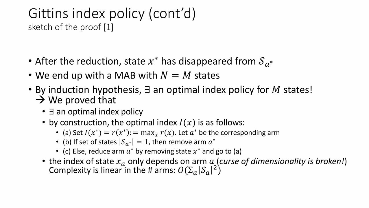
• After the reduction, state 𝑥∗ has disappeared from 𝒮𝑎∗

• We end up with a MAB with 𝑁 = 𝑀 states

• By induction hypothesis, ∃ an optimal index policy for 𝑀 states!We proved that • ∃ an optimal index policy• by construction, the optimal index 𝐼(𝑥) is as follows:

• (a) Set 𝐼(𝑥∗) = 𝑟 𝑥∗ : = max𝑥 𝑟(𝑥). Let 𝑎∗ be the corresponding arm• (b) If set of states 𝑆𝑎∗ = 1, then remove arm 𝑎∗

• (c) Else, reduce arm 𝑎∗ by removing state 𝑥∗ and go to (a)

• the index of state 𝑥𝑎 only depends on arm 𝑎 (curse of dimensionality is broken!)Complexity is linear in the # arms: 𝑂(Σ𝑎 𝒮𝑎

2)

Gittins index policy (cont’d)sketch of the proof [1]

Gittins indexFurther intuitions

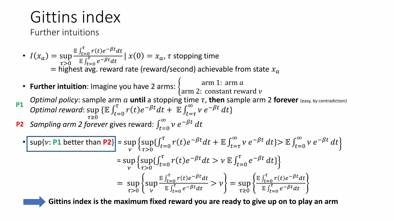
• 𝐼 𝑥𝑎 = sup𝜏>0

𝔼 ∫𝑡=0𝜏

𝑟 𝑡 𝑒−𝛽𝑡𝑑𝑡

𝔼 ∫𝑡=0𝜏

𝑒−𝛽𝑡𝑑𝑡| 𝑥 0 = 𝑥𝑎, 𝜏 stopping time

= highest avg. reward rate (reward/second) achievable from state 𝑥𝑎

• Further intuition: Imagine you have 2 arms: ቊ arm 1: arm 𝑎arm 2: constant reward 𝜈

Optimal policy: sample arm 𝑎 until a stopping time 𝜏, then sample arm 2 forever (easy, by contradiction)

Optimal reward: sup𝜏≥0

{𝔼∫𝑡=0𝜏

𝑟 𝑡 𝑒−𝛽𝑡𝑑𝑡 + 𝔼∫𝑡=𝜏∞

𝜈 𝑒−𝛽𝑡 𝑑𝑡}

Sampling arm 2 forever gives reward: ∫𝑡=0∞

𝜈 𝑒−𝛽𝑡 𝑑𝑡

• sup{𝜈: P1 better than P2} = sup𝜈

sup𝜏>0

{∫𝑡=0𝜏

𝑟 𝑡 𝑒−𝛽𝑡𝑑𝑡 + 𝔼∫𝑡=𝜏∞

𝜈 𝑒−𝛽𝑡 𝑑𝑡}> 𝔼∫𝑡=0∞

𝜈 𝑒−𝛽𝑡 𝑑𝑡

= sup𝜈

sup𝜏>0

{∫𝑡=0𝜏

𝑟 𝑡 𝑒−𝛽𝑡𝑑𝑡 > 𝜈 𝔼∫𝑡=0𝜏

𝑒−𝛽𝑡 𝑑𝑡}

= sup𝜏>0

sup𝜈

𝔼 ∫𝑡=0𝜏

𝑟 𝑡 𝑒−𝛽𝑡𝑑𝑡

𝔼 ∫𝑡=0𝜏

𝑒−𝛽𝑡𝑑𝑡> 𝜈 = sup

𝜏≥0

𝔼 ∫𝑡=0𝜏

𝑟 𝑡 𝑒−𝛽𝑡𝑑𝑡

𝔼 ∫𝑡=0𝜏

𝑒−𝛽𝑡𝑑𝑡

Gittins index is the maximum fixed reward you are ready to give up on to play an arm

P1

P2

Frequentist model

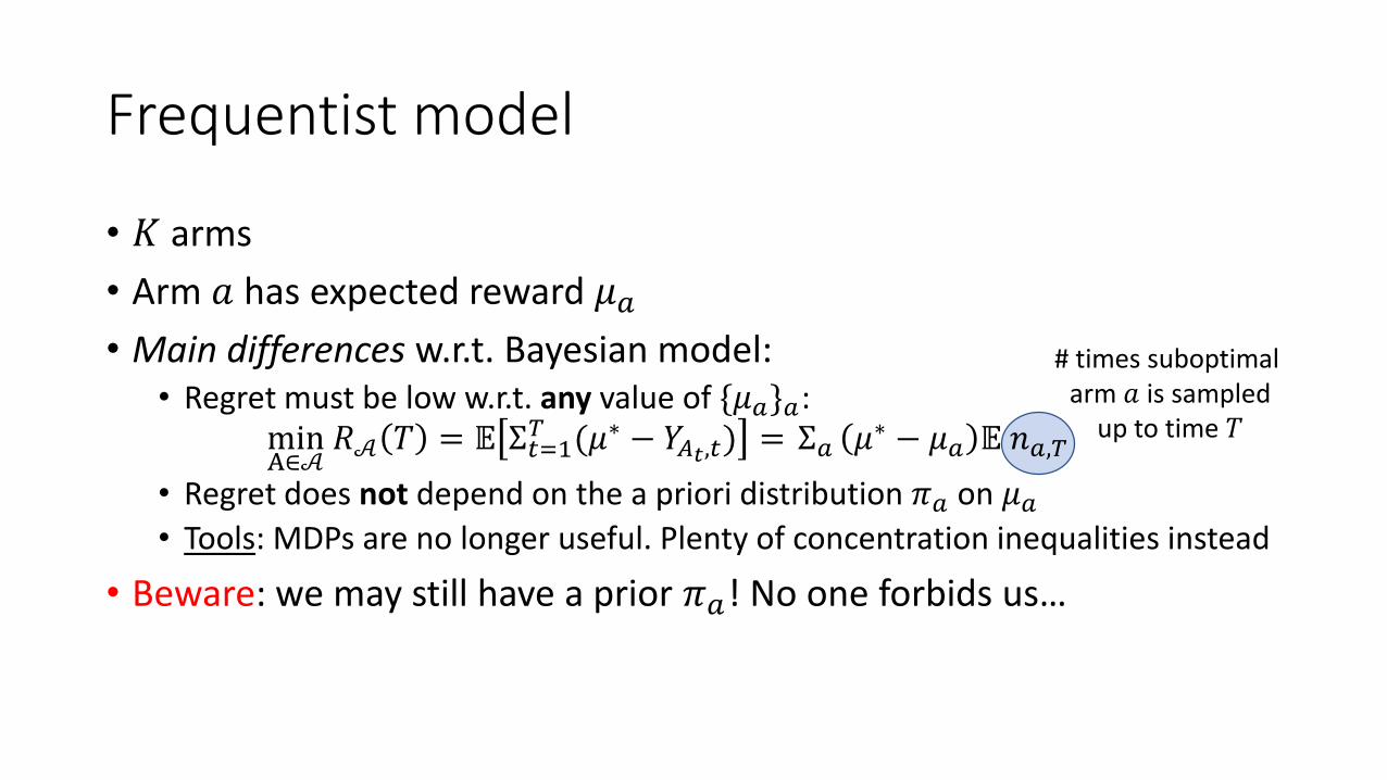
Frequentist model

• 𝐾 arms

• Arm 𝑎 has expected reward 𝜇𝑎• Main differences w.r.t. Bayesian model:

• Regret must be low w.r.t. any value of {𝜇𝑎}𝑎:minA∈𝒜

𝑅𝒜 𝑇 = 𝔼 Σ𝑡=1𝑇 (𝜇∗ − 𝑌𝐴𝑡,𝑡) = Σ𝑎 𝜇∗ − 𝜇𝑎 𝔼 𝑛𝑎,𝑇

• Regret does not depend on the a priori distribution 𝜋𝑎 on 𝜇𝑎• Tools: MDPs are no longer useful. Plenty of concentration inequalities instead

• Beware: we may still have a prior 𝜋𝑎! No one forbids us…

# times suboptimal arm 𝑎 is sampled

up to time 𝑇

A famous frequentist algorithm:

Upper Confidence Bound (UCB)

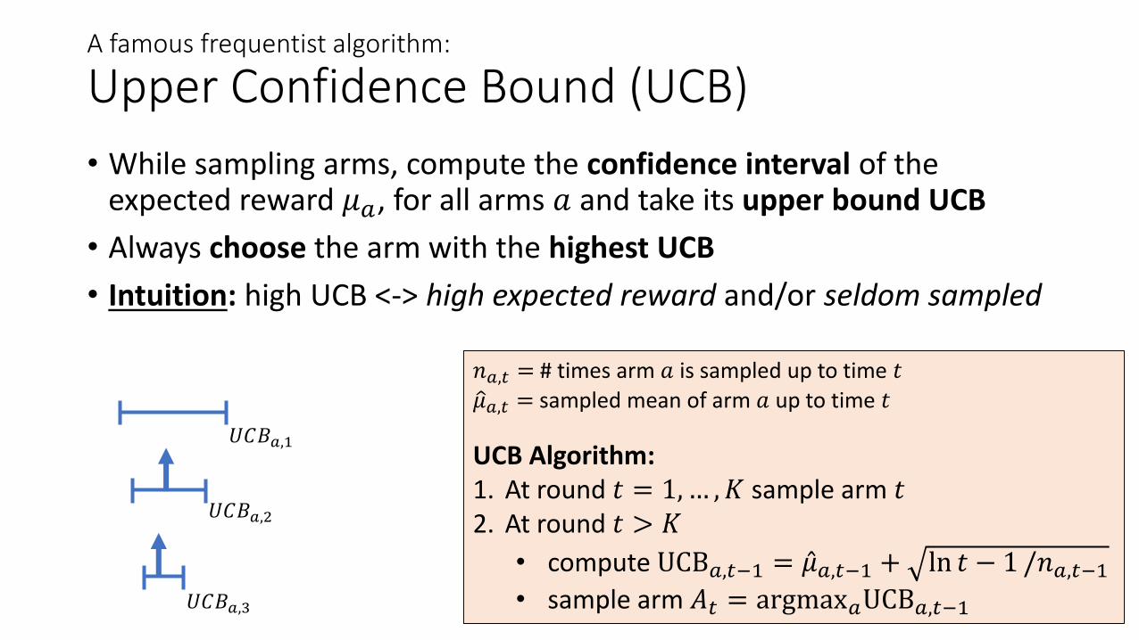
• While sampling arms, compute the confidence interval of the expected reward 𝜇𝑎, for all arms 𝑎 and take its upper bound UCB

• Always choose the arm with the highest UCB

• Intuition: high UCB <-> high expected reward and/or seldom sampled

𝑈𝐶𝐵𝑎,1

𝑈𝐶𝐵𝑎,2

𝑈𝐶𝐵𝑎,3

𝑛𝑎,𝑡 = # times arm 𝑎 is sampled up to time 𝑡

ො𝜇𝑎,𝑡 = sampled mean of arm 𝑎 up to time 𝑡

UCB Algorithm:1. At round 𝑡 = 1,… , 𝐾 sample arm 𝑡2. At round 𝑡 > 𝐾

• compute UCB𝑎,𝑡−1 = Ƹ𝜇𝑎,𝑡−1 + ln 𝑡 − 1 /𝑛𝑎,𝑡−1• sample arm 𝐴𝑡 = argmax𝑎UCB𝑎,𝑡−1

Upper Confidence Bound (UCB)

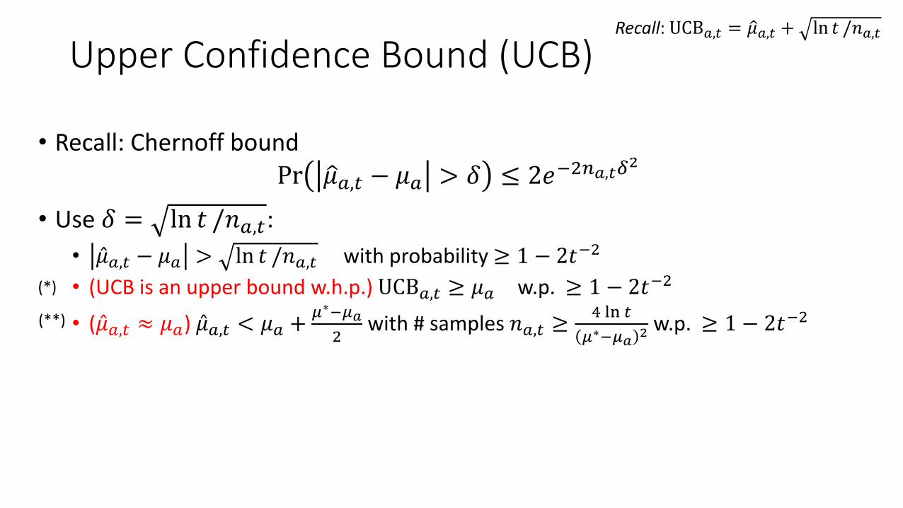
• Recall: Chernoff bound

Pr ො𝜇𝑎,𝑡 − 𝜇𝑎 > 𝛿 ≤ 2𝑒−2𝑛𝑎,𝑡𝛿2

• Use 𝛿 = ln 𝑡 /𝑛𝑎,𝑡:

• Ƹ𝜇𝑎,𝑡 − 𝜇𝑎 > ln 𝑡 /𝑛𝑎,𝑡 with probability ≥ 1 − 2𝑡−2

• (UCB is an upper bound w.h.p.) UCB𝑎,𝑡 ≥ 𝜇𝑎 w.p. ≥ 1 − 2𝑡−2

• ( Ƹ𝜇𝑎,𝑡 ≈ 𝜇𝑎) Ƹ𝜇𝑎,𝑡 < 𝜇𝑎 +𝜇∗−𝜇𝑎

2with # samples 𝑛𝑎,𝑡 ≥

4 ln 𝑡

𝜇∗−𝜇𝑎2 w.p. ≥ 1 − 2𝑡−2

Recall: UCB𝑎,𝑡 = ො𝜇𝑎,𝑡 + ln 𝑡 /𝑛𝑎,𝑡

(*)

(**)

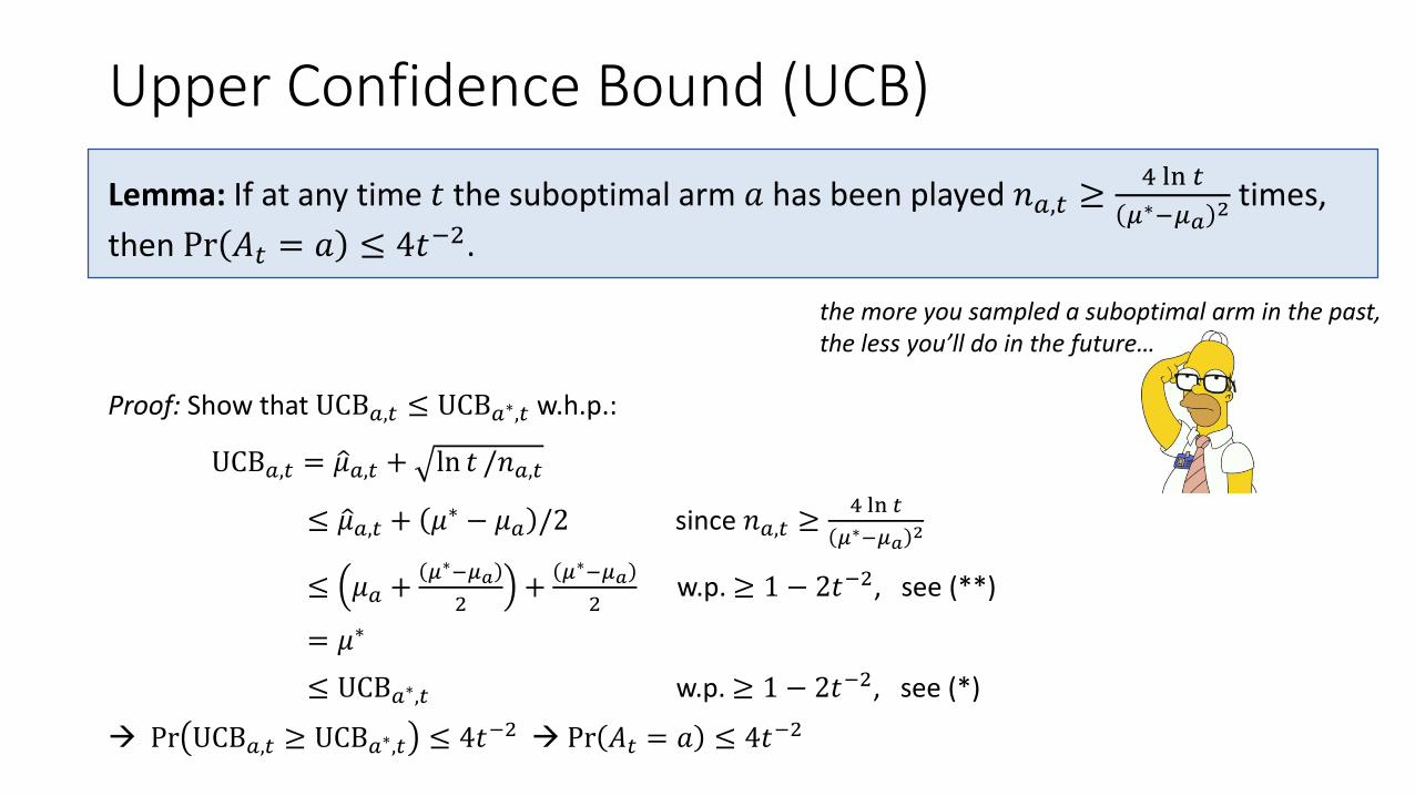
Lemma: If at any time 𝑡 the suboptimal arm 𝑎 has been played 𝑛𝑎,𝑡 ≥4 ln 𝑡

𝜇∗−𝜇𝑎2 times,

then Pr 𝐴𝑡 = 𝑎 ≤ 4𝑡−2.

Proof: Show that UCB𝑎,𝑡 ≤ UCB𝑎∗,𝑡 w.h.p.:

UCB𝑎,𝑡 = ො𝜇𝑎,𝑡 + ln 𝑡 /𝑛𝑎,𝑡

≤ ො𝜇𝑎,𝑡 + 𝜇∗ − 𝜇𝑎 /2 since 𝑛𝑎,𝑡 ≥4 ln 𝑡

𝜇∗−𝜇𝑎2

≤ 𝜇𝑎 +𝜇∗−𝜇𝑎

2+

𝜇∗−𝜇𝑎

2w.p. ≥ 1 − 2𝑡−2, see (**)

= 𝜇∗

≤ UCB𝑎∗,𝑡 w.p. ≥ 1 − 2𝑡−2, see (*)

Pr UCB𝑎,𝑡 ≥ UCB𝑎∗,𝑡 ≤ 4𝑡−2 Pr 𝐴𝑡 = 𝑎 ≤ 4𝑡−2

Upper Confidence Bound (UCB)

the more you sampled a suboptimal arm in the past,the less you’ll do in the future…

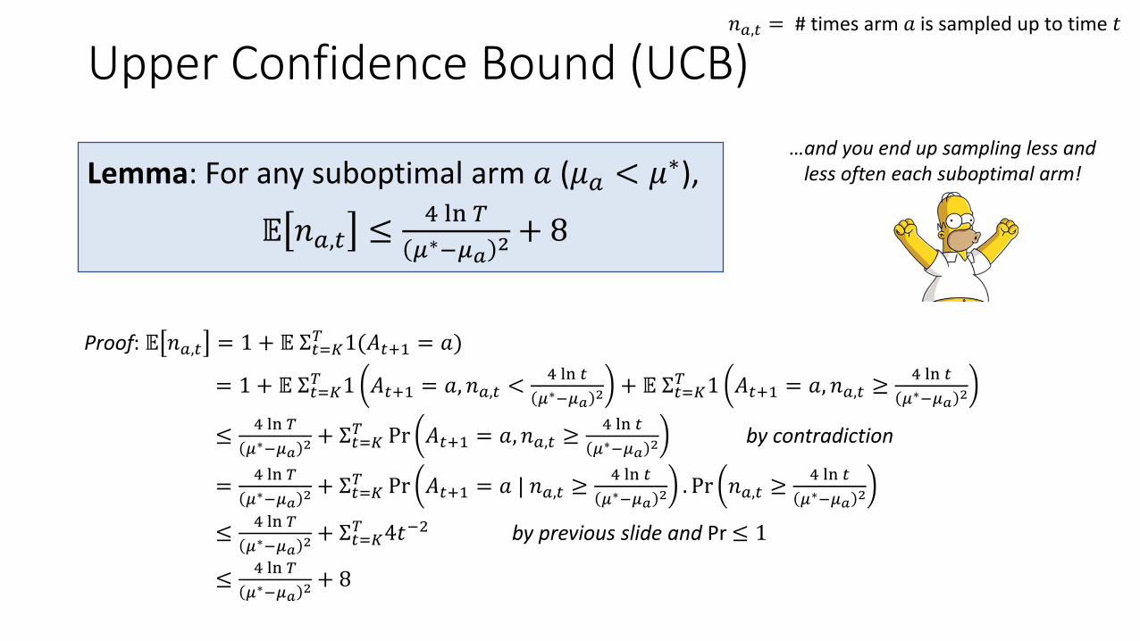
Lemma: For any suboptimal arm 𝑎 (𝜇𝑎 < 𝜇∗),

𝔼 𝑛𝑎,𝑡 ≤4 ln 𝑇

𝜇∗−𝜇𝑎2 + 8

Upper Confidence Bound (UCB)𝑛𝑎,𝑡 = # times arm 𝑎 is sampled up to time 𝑡

…and you end up sampling less and less often each suboptimal arm!

Proof: 𝔼 𝑛𝑎,𝑡 = 1 + 𝔼 Σ𝑡=𝐾𝑇 1(𝐴𝑡+1 = 𝑎)

= 1 + 𝔼 Σ𝑡=𝐾𝑇 1 𝐴𝑡+1 = 𝑎, 𝑛𝑎,𝑡 <

4 ln 𝑡

𝜇∗−𝜇𝑎2 + 𝔼 Σ𝑡=𝐾

𝑇 1 𝐴𝑡+1 = 𝑎, 𝑛𝑎,𝑡 ≥4 ln 𝑡

𝜇∗−𝜇𝑎2

≤4 ln 𝑇

𝜇∗−𝜇𝑎2 + Σ𝑡=𝐾

𝑇 Pr 𝐴𝑡+1 = 𝑎, 𝑛𝑎,𝑡 ≥4 ln 𝑡

𝜇∗−𝜇𝑎2 by contradiction

=4 ln 𝑇

𝜇∗−𝜇𝑎2 + Σ𝑡=𝐾

𝑇 Pr 𝐴𝑡+1 = 𝑎 | 𝑛𝑎,𝑡 ≥4 ln 𝑡

𝜇∗−𝜇𝑎2 . Pr 𝑛𝑎,𝑡 ≥

4 ln 𝑡

𝜇∗−𝜇𝑎2

≤4 ln 𝑇

𝜇∗−𝜇𝑎2 + Σ𝑡=𝐾

𝑇 4𝑡−2 by previous slide and Pr ≤ 1

≤4 ln 𝑇

𝜇∗−𝜇𝑎2 + 8

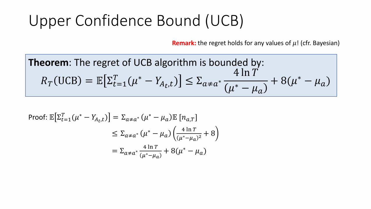
Theorem: The regret of UCB algorithm is bounded by:

𝑅𝑇 UCB = 𝔼 Σ𝑡=1𝑇 (𝜇∗ − 𝑌𝐴𝑡,𝑡) ≤ Σ𝑎≠𝑎∗

4 ln 𝑇

𝜇∗ − 𝜇𝑎+ 8(𝜇∗ − 𝜇𝑎)

Proof: 𝔼 Σ𝑡=1𝑇 (𝜇∗ − 𝑌𝐴𝑡,𝑡) = Σ𝑎≠𝑎∗ 𝜇∗ − 𝜇𝑎 𝔼 [𝑛𝑎,𝑇]

≤ Σ𝑎≠𝑎∗ 𝜇∗ − 𝜇𝑎4 ln 𝑇

𝜇∗−𝜇𝑎2 + 8

= Σ𝑎≠𝑎∗4 ln 𝑇

𝜇∗−𝜇𝑎+ 8(𝜇∗ − 𝜇𝑎)

Upper Confidence Bound (UCB)Remark: the regret holds for any values of 𝜇! (cfr. Bayesian)

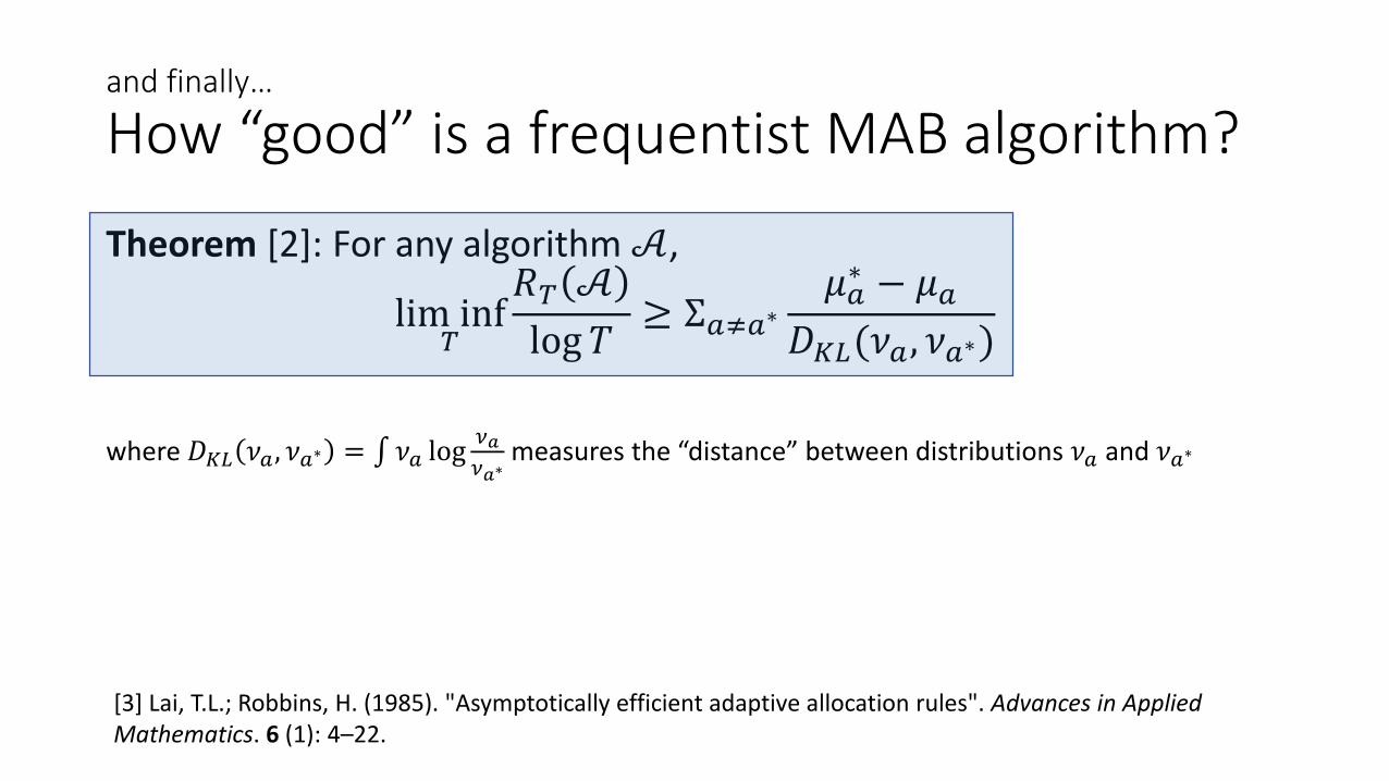
and finally…

How “good” is a frequentist MAB algorithm?

Theorem [2]: For any algorithm 𝒜,

lim inf𝑇

𝑅𝑇 𝒜

log 𝑇≥ Σ𝑎≠𝑎∗

𝜇𝑎∗ − 𝜇𝑎

𝐷𝐾𝐿(𝜈𝑎, 𝜈𝑎∗)

where 𝐷𝐾𝐿 𝜈𝑎, 𝜈𝑎∗ = ∫𝜈𝑎 log𝜈𝑎

𝜈𝑎∗measures the “distance” between distributions 𝜈𝑎 and 𝜈𝑎∗

[3] Lai, T.L.; Robbins, H. (1985). "Asymptotically efficient adaptive allocation rules". Advances in Applied Mathematics. 6 (1): 4–22.

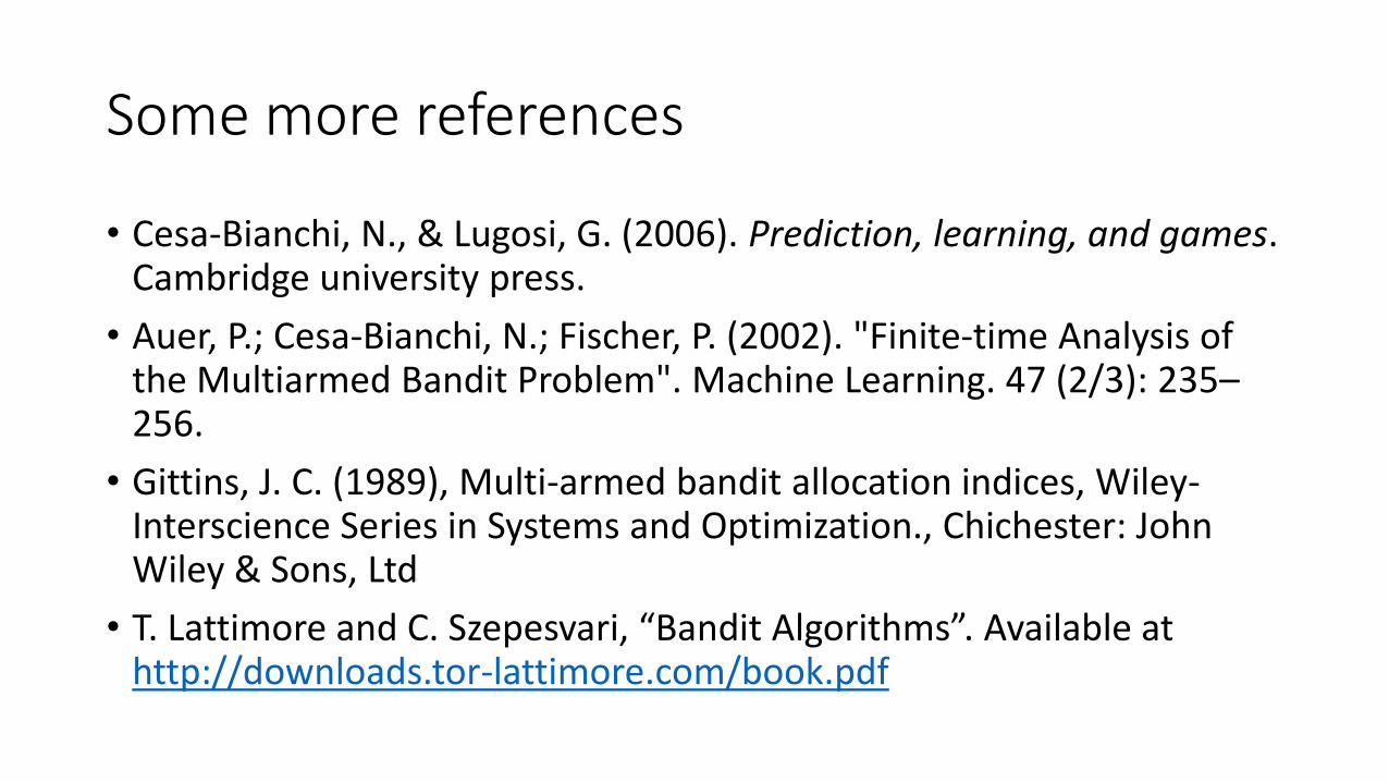
Some more references

• Cesa-Bianchi, N., & Lugosi, G. (2006). Prediction, learning, and games. Cambridge university press.

• Auer, P.; Cesa-Bianchi, N.; Fischer, P. (2002). "Finite-time Analysis of the Multiarmed Bandit Problem". Machine Learning. 47 (2/3): 235–256.

• Gittins, J. C. (1989), Multi-armed bandit allocation indices, Wiley-Interscience Series in Systems and Optimization., Chichester: John Wiley & Sons, Ltd

• T. Lattimore and C. Szepesvari, “Bandit Algorithms”. Available at http://downloads.tor-lattimore.com/book.pdf