Bayesian Population Forecasting: Extending the Lee-Carter … · Bayesian Population Forecasting: Extending the Lee-Carter Method Arkadiusz Wiśniowski1 & PeterW.F.Smith1 & Jakub

Bayesian Population Forecasting: Extendingthe Lee-Carter Method

Arkadiusz Wiśniowski1 & Peter W. F. Smith1&

Jakub Bijak1& James Raymer2 &

Jonathan J. Forster1

Published online: 12 May 2015# The Author(s) 2015. This article is published with open access at Springerlink.com

Abstract In this article, we develop a fully integrated and dynamic Bayesian approach toforecast populations by age and sex. The approach embeds the Lee-Carter type modelsfor forecasting the age patterns, with associated measures of uncertainty, of fertility,mortality, immigration, and emigration within a cohort projection model. The method-ology may be adapted to handle different data types and sources of information. Toillustrate, we analyze time series data for the United Kingdom and forecast the compo-nents of population change to the year 2024. We also compare the results obtained fromdifferent forecast models for age-specific fertility, mortality, and migration. In doing so,we demonstrate the flexibility and advantages of adopting the Bayesian approach forpopulation forecasting and highlight areas where this work could be extended.

Keywords Bayesian . Lee-Carter model . Population forecasting . uncertainty .

UnitedKingdom

Introduction

This work is guided by two aims. The first is to have a flexible platform for forecastingpopulations. Most statistical offices in developed countries utilize data obtained from

Demography (2015) 52:1035–1059DOI 10.1007/s13524-015-0389-y

Electronic supplementary material The online version of this article (doi:10.1007/s13524-015-0389-y)contains supplementary material, which is available to authorized users.

* Arkadiusz Wiś[email protected]

1 Economic and Social Research Council Centre for Population Change, University of Southampton,Highfield, SO17 1BJ Southampton, UK

2 Australian Demographic & Social Research Institute, The Australian National University,Acton ACT 2601, Australia

http://dx.doi.org/10.1007/s13524-015-0389-y

different sources, including administrative registers, surveys, and censuses with varyinglevels of quality and measurement. Cohort component models have long been thestandard apparatus for producing projections, but wide differences remain in theunderlying assumptions, especially regarding the treatment of migration and the levelof detail provided. The forecasting approach we have developed is one that can beadapted to include all demographic components of change by age and sex, and providesmeasures of the accuracy of the forecasts.

As we move away from deterministic population projections to those that providemeasures of uncertainty, we believe it is important to integrate the various sources ofuncertainty into the modeling framework. The rationale for considering a Bayesianapproach is that it offers a natural probabilistic framework to predict future populations.Variability in the data and uncertainties in the parameters and model choice can beexplicitly incorporated by using probability distributions, and the predictive distribu-tions follow directly from the probabilistic model applied. The approach also allows theinclusion of expert judgments, together with their uncertainty, in the model framework.

The second aim of this article is to provide a flexible and consistent method forforecasting the age patterns of fertility, mortality, and migration that drive our forecastresults. A vast literature focuses on modeling demographic events (e.g., Bongaarts andBulatao 2000), but approaches for forecasting the age patterns are less abundant.Methods for forecasting migration, in particular, represent a persistent weakness inpopulation forecast models (Bijak 2010).

Our population forecasting model is developed with these two aims in mind. Wefocus on generalizing and extending the Lee-Carter model for forecasting mortality toage-specific fertility and migration (Lee and Carter 1992), and integrating these into thecohort projection mechanism. One of the contributions of the proposed approach isforecasting age-specific emigration rates and immigration volumes, following thesuggestions of Rees (1986:148). Because the age patterns of immigration and emigra-tion are more regular than those observed for net migration, they are better amenable tomodeling by using Lee-Carter models.

Background

Forecasting the Age Patterns of Fertility, Mortality, and Migration

There is a long history of modeling the age patterns of fertility, mortality, and migrationevents (Booth 2006). This work has demonstrated the persistent and strong regularitiesin the age patterns over time and across space (Preston et al. 2001:191–210; Rogers1986; Rogers and Little 1994) driven by biological and social life course mechanisms(Courgeau 1985). The age regularities exhibited in demographic patterns allow popu-lation forecasters to simplify their underlying assumptions and models. Indeed, someforecasts focus on indicator variables, such as the total fertility rate (TFR), lifeexpectancy, or net migration rate, which are then converted into an assumed agedistribution (see, e.g., Raftery et al. 2012; Wilson and Bell 2007).

The main approaches for modeling the age patterns of demographic componentsinclude the imposition of empirical tables obtained from other countries and historicalsettings (Coale and Demeny 1966), parametric model schedules (Coale and McNeil

1036 A. Wiśniowski et al.

1972; Coale and Trussell 1974; Heligman and Pollard 1980; Knudsen et al. 1993;Rogers 1986; Rogers and Castro 1981; Rogers et al. 1978), relational models (Brass1974), functional models (De Beer 2011; Hyndman and Booth 2008; Hyndman andUllah 2007; Lee and Carter 1992), and hierarchical Bayesian models (Czado et al.2005; Girosi and King 2008). Of these, the most successful and widely used forforecasting future patterns and uncertainty have been the relational and functionalmodels—particularly, the Lee-Carter model for mortality (Booth and Tickle 2008).

Relational and functional models include standards or time-invariant patterns,which are then perturbed based on a set of parameters. Because the shapes of age-specific fertility, mortality, and migration largely remain the same over time, theseapproaches provide a powerful tool for forecasting. In the Lee-Carter case, single-or five-year age groups are altered on the basis of time series equations. The maincritique of the original Lee-Carter approach is that it can produce implausibleforecasts for particular age groups (see Girosi and King 2008:38–42). As aconsequence, several extensions have been developed to accommodate cohorteffects, correlation between sexes, and smoothing (Booth and Tickle 2008; Lee2000), as well as to forecast fertility rates (Lee 1993).

Bayesian Population Forecasting

The need to incorporate probabilistic uncertainty into population estimates and fore-casts is well known. Probabilistic forecasts have the advantage over variant styleprojections in that they specify the chances or probability that a particular futurepopulation value will be within any given range (Ahlburg and Land 1992; Alho andSpencer 1985, 2005; Bongaarts and Bulatao 2000; Keilman 1990; Lee and Tuljapurkar1994; Lutz 1996). With variant projections, on the other hand, the user has no idea howlikely future population values are, but only that they are plausible scenariosrepresenting the “most likely” and the “extreme” high and low possibilities.However, despite the known advantages of probabilistic forecasts, they have yet tobe widely adopted by statistical agencies (Lutz and Goldstein 2004). The reason is thatthere are many types of uncertainties to consider, and including them in projections isnot always straightforward.

According to Alho (1999), probabilistic population forecasting within the Bayesianframework has a tradition dating back over 60 years to the seminal works of LeoTörnqvist and colleagues (Hyppölä et al. 1949). However, it was not until the 1980sthat probabilistic methods began entering mainstream demography. These includedtime series extrapolations, expert-based forecasting, and past error propagation (for adetailed overview of different approaches, see Bijak 2010). Examples of Bayesianmodels for population forecasting were practically non-existent until the past few years,with the notable exception of Daponte et al. (1997). Recent advances in fastcomputation and numerical methods have enabled a more widespread use of theBayesian approach in many fields of application, including population forecasting. Ata global level, Raftery et al. (2012) proposed a generic model for all countries of theworld, based on aggregate indicators (TFRs and life expectancies) and model lifetables. At the opposite end of the data spectrum, Bryant and Graham (2013) suggesteda comprehensive Bayesian approach to reconcile different data sources for NewZealand, a country with very good availability of population statistics.

Bayesian Population Forecasting 1037

Bryant and Graham’s (2013) approach uses an accounting framework forestimating New Zealand’s current population disaggregated by regions, age, sexand time. It combines various data sources, including vital events registers,censuses, and school and electoral rolls. The model constrains the true valuesof the demographic components by the population accounting equation. Also,age, time, sex and regional patterns are specified by main effect and two-wayinteraction terms within a Poisson-gamma model, similar to non-Bayesianapproaches of Smith et al. (2010) and Raymer et al. (2011b).

Concurrently, Wheldon et al. (2013) undertook Bayesian estimation andprojection of populations to reconstruct past population data. Their approachis based on modeling the three population components—fertility, mortality, andnet migration—and accounts for the varying quality of the population figuresavailable from the censuses. Census data are treated as biased estimates of thetrue unknown population count. Their approach does not provide a systematicmodeling of the age profiles and does not account for changing behaviors overtime. The information about the model parameters is fed into the model in theform of the informative prior distributions. The component forecasts areinserted in the cohort-component model similar to the one described in theupcoming subsection on the population projection model.

Methodology

In this section, we first introduce the forecasting model proposed by Lee and Carter(1992) and then describe how it can be extended and applied within a Bayesianframework. The Lee-Carter model was originally designed to forecast age-specificmortality rates with the following specification:

logμx;t ¼ αx þ βxκt þ ξx;t; ð1Þwhere the logarithm of the age and time-specific mortality rate μx,t isdecomposed into an overall age profile, αx, averaged over the entire periodunder consideration, and age-specific changes in mortality βx. The subscripts xand t denote age and time, respectively. The βx parameter describes how fastthe rates decline over time in response to changes in the time-specific effect κt.The error term ξx,t is assumed to be normally distributed with a mean of 0 anda constant variance. To forecast mortality rates into the future, a simple randomwalk with drift model for κt was proposed:

κt ¼ ϕþ κt−1 þ εt: ð2ÞTo ensure identifiability of the model parameters, constraints are imposed suchthat a sum of βx over age is 1 and a sum of κt over time is 0 (Lee and Carter1992:661). Lee (1993) subsequently proposed a similar model to forecast age-specific fertility for the United States. In that model, several constraints wereintroduced to represent the prior information on fertility.

In this article, we extend and adapt the Lee-Carter model to create a generalframework for forecasting mortality, fertility, emigration and immigration. In this


framework, we first assume that count data on a given population component Yx,tg,k

follow a Poisson distribution:

Yg;kx;t ePoisson μg;k

x;t Rg;kx;t

� �; ð3Þ

where g ∈ {D,B,E,I} denotes a component of population change: D representsdeaths (mortality), B is births (fertility), E is emigration, I is immigration, sex k =F denotes females, and k = M stands for males. Parameter μx,t

g,k denotes a ratio ofcounts of demographic event scaled to the size of the population exposed to riskof these events, Rx,t

g,k. As in the original Lee-Carter model, t and x denote time andage, respectively. For mortality and emigration, the population at risk is the same;for fertility, it consists of women of reproductive age. For immigration, we forecastthe counts rather than rates; hence, we assume that Rx,t

I,k = 1 for all x, t, and k.Czado et al. (2005) developed the extension of the Lee-Carter model to incorporatePoisson variability of death counts within the Bayesian framework.

Second, we assume that the logarithm of the rate follows a normal distribution:

logμg;kx;t e N αg;k

x þ βg;kx κg;kt þ γg;kt−x; τ

g;k� �

; ð4Þ

where αxg,k, βx

g,k, and κtg,k represent the same parameters as in the Lee-Carter model, and

γt− xg,k denotes a cohort effect. The cohort effect, introduced by Renshaw and Haberman

(2006) for mortality, is incorporated in our framework for the sake of generality, but itmay be omitted if not required. Throughout this article, N(μ,τ) denotes a normaldistribution with a mean of μ and precision (inverse variance) τ. The normal distribu-tion assumed for rates is an extension of the Czado et al. (2005) model. It allowscapturing the overdispersion that is not explained by the variability resulting from thePoisson sampling of count data.

Third, for the time-specific effects, κtg,k, we require a time series model,

which facilitates the forecasting. This model can be univariate, such as randomwalk with drift in the original Lee-Carter specification, for each component andeach sex; alternatively, the model can be multivariate (e.g., vectorautoregression (VAR)), which allows exploring correlations between sexes andcomponents. A time series model is also utilized for a cohort effect, γt − x

g,k . Inour application, we use a univariate model. However, more general multivariateframeworks can be used.

To ensure identification of the parameters αxg,k, βx

g,k, κtg,k, and γt− x

g,k , the followingconstraints are imposed:

Xz

x ¼ 0

βg;kx ¼ 1; κg;k1 ¼ 0; γg;k1 ¼ 0; ð5Þ

where z denotes the oldest age group. These constraints suffice to identify the bilinearmodel in Eq. (4) as long as there is a clear differentiation in the βx—that is, as long asthey are not all equal to 1 / z, in which case the model reduces to the linear age-period-cohort (APC) model. The problem of identification of the period and cohort effects inthe APC model has long been discussed in the literature (see Luo 2013, with acomment by Fienberg 2013).


To learn about the model parameters, and specifically about the forecasts of thepopulation components, we use Bayesian inference. Bayes theorem states that theposterior distribution of the model parameters (e.g., forecasts of the age-specificmortality rates) is proportional to the product of the likelihood for the data and theprior distribution. In our approach, Bayesian inference integrates uncertainty from thedemographic event (count) data expressed by the Poisson likelihood with weaklyinformative prior distributions that give preference to the historical data.Subsequently, all four components of population change are combined within thecohort component projection model.

In the following subsections, we present specific adaptations of the precedingframework to forecast mortality, fertility, and migration. We adopt a convention ofproposing a very simple model for the data (such as the original Lee-Carter model)with a more general one. Because our extensions of the Lee-Carter model lead to arelatively complex specification of the probabilistic model, the closed forms of theposterior distributions are difficult to obtain analytically. Hence, we sample fromthe posterior distributions by using the Markov chain Monte Carlo (MCMC)algorithms implemented in the OpenBUGS software (Lunn et al. 2009). The examplecode used for the simulations for fertility is available in Online Resource 1 (section A.3).The other codes are available from the corresponding author upon request.

Forecasting Mortality

To forecast the mortality of males and females, we consider the Bayesian version of theoriginal Lee-Carter model, denoted as M1, and a general extension of this model,denoted by M2. The Lee-Carter model M1 is specified as in Eqs. (1) and (2), and theage-specific mortality rates are calculated as μx,t

D,k=Yx,tD,k / Rx,t

D,k. Model M2 for deathcounts Yx,t

D,k follows Eqs. (3) and (4).In M1, the time-specific parameters κt

k (we drop the superscriptD for each parameterfor clarity of notation) follow univariate random walk with drift models, as in theoriginal Lee-Carter specification. In M2, κt

k for both sexes follow a bivariate vectorautoregressive VAR(1) process with drift:

κFt

κMt

� �eMNV 2

ϕ01

ϕ02

� �þ ϕ11 ϕ12

ϕ21 ϕ22

� �κFt−1

κMt−1

� �;Tκ

� �; ð6Þ

where MVN2 denotes a two-dimensional multivariate normal distribution, with theprecision matrix Tκ; ϕij, i, j = 1, 2 are the parameters of the VAR(1) model, withϕ0j, j = 1, 2 being drift terms. The instantaneous and lagged correlations assumed formales and females reflect the assumption of parallel improvements in health conditionsover time. 1 Finally, the cohort effect γt − x

k for each sex k follows a univariateautoregressive process AR(1) with parameters ψ0

k and ψ1k:

γkt−x e N ψk0 þ ψk

1γkt−x−1; τ

kγ

� �: ð7Þ

1 Li and Lee (2005) proposed an alternative approach to include correlations between sexes; they added acommonality factor to Eq. (1).


Forecasting Fertility

For forecasting age-specific fertility rates, we apply a simple version of the Lee (1993)model, here called F1. The extended model, denoted by F2, includes a cohort effect(see also Cheng and Lin 2010; Lee 1993, 2000). The population at risk represents allwomen of reproductive age.

The time component in F1 follows an ARMA (1,1) process (again we suppress thesuperscripts B and k because the model relates only to females):

κt e N ϕ0 þ ϕ1 κt−1 − ϕ0ð Þ þ ϕ2ξt−1; τκð Þ; ð8Þwhere ξt = κt−ϕ0−ϕ1(κt−1−ϕ0)−ϕ2ξt−1.

In Model F2, we use a simple univariate autoregressive process AR(1) for the timecomponent κt and for γt−x:

κt ∼ N ϕ0 þ ϕ1κt−1; τκð Þ ;γt−x ∼ N ψ0 þ ψ1γt−x−1; τγ

� :

ð9Þ

Forecasting Immigration Counts and Emigration Rates

To forecast immigration counts and emigration rates, we introduce two models: (1) aunivariate model, denoted by IE1, which assumes no correlation between emigrationand immigration of males and females; and (2) a multivariate model, denoted by IE2, inwhich we assume correlation between the time parameters κt for both sexes and bothdirections of migration. In both models, we incorporate smoothing, built in into theprior distributions for the age-specific model parameters αx and βx. Unlike mortalityand fertility, there is no clear rationale for including a cohort effect parameter inforecasting immigration and emigration. Also, because immigration does not have aneasily defined population at risk, we model the counts, which is a common practice inpopulation projections (McDonald and Kippen 2002; Rees 1986).

In IE1, we assume a random walk without drift for emigration rates and immigrationcounts for both sexes:

κg;kt e N κg;kt−1; τg;kκ

� �: ð10Þ

This simple model leads to forecasts with a constant expectation (as the last observa-tion) and increasing uncertainty.

For IE2, we assume instantaneous correlation in the time parameters for emigrationand immigration for both sexes:

κt e MVN 4 ϕ0 þϕ1log tð Þ þϕ2t þ ∘ϕ3κt−1;Tκ½ �; ð11Þ

where κt = (κtE,F, κt

E,M, κtI,F, κt

I,M)′, ϕi = (ϕi1, . . . ,ϕi4)′, Tκ is a precision matrix, (∘)denotes element-wise multiplication, and the prime notation (′) denotes transposition.We simplify the model by having the time parameters, κt, depend only on their ownlagged values and not on the direction of the flow. This model includes a drift termϕ0,an autoregressive parameter ϕ3, a logarithmic trend with parameter ϕ1, and a lineartrend with parameter ϕ2.


Prior Distributions

In the absence of any prior information, we suggest using weakly informative distri-butions that will allow the data to drive the estimation. For the general forecastingmodel, we propose a set of priors, the hyperparameters of which may differ in particularapplications. For both sexes k, the specifications of the prior distributions for the modelparameters are as follows:

αkx e N 0; 0:01ð Þ f or all x ;

βk1:z−1 e MVNz−1 1 = z; τkβΨ

kβ

� �; βk

z ¼ 1−Xz−1i¼1

βkx;

τkβ e Γ 0:001; 0:001ð Þ;ϕi j ∼ N 0; 1ð Þ; for all i and j;

ψki ∼ N 0; 1ð Þ; i ¼ 0; 1;

σk ∼ U 0; 100ð Þ; τk ¼ σk� −2

; σkγ ∼ > U 0; 100ð Þ; τkγ ¼ σk

γ

� �−2;

Tκ ∼ Wishart lIl; lð Þ;

ð12Þ

where Γ(a,b) denotes the gamma distribution with a mean of a / b and variance a / b2;Udenotes uniform distribution; andΨβ

k is a precision matrix for a conditional distributionof βx, given that they sum to 1 (details are presented in Online Resource 1, section A.2).The preceding prior distributions imply weak information a priori about the modelparameters. For the age-specific parameters αx and βx, we avoid specifications based onthe data (i.e., the empirical Bayes approach) suggested by Czado et al. (2005). For theprecision parameters τk and τγ

k, we follow Gelman’s (2006) suggestions of avoidingconjugate gamma distributions, and we use uniform priors for standard deviations over alarge range. TheWishart distribution is a standard prior distribution for precision matrixin the multivariate time series model and is easy to implement in the OpenBUGSsoftware. The subscript l denotes the number of series in the model: males and femalesfor mortality (i.e., l = 2) or male and female migration in both directions (i.e., l = 4). Inthe univariate model (e.g., for fertility or for a single sex), we replace the Wishart priorwith a uniform prior for the standard deviation; that is, σκ ~ U(0,100),τκ=(σκ)

−2.For low-quality data, smoothing of the age profile may be required. In this case, we

propose a smoothing technique that is embedded in the specification of the priordistributions for parameters αx and βx. Smoothing prevents the artificial age patternsresulting from the sample data from being propagated in the forecasts. Our smoothingmethod is based on the spatial autoregressive processes (see, e.g., Besag 1986).

Prior densities for smoothing the age-specific parameters αx are constructed in thefollowing way, with the sex and population component superscripts omitted for clarity.For the youngest and oldest age groups, we assume that the mean of the priordistribution depends on the second-youngest and second-oldest group, respectively:

α0 e N α1;1

2τα

� �; αz e N αz−1;

1

2τα

� �: ð13Þ


For the remaining age groups, we assume that their means depend on the average of thetwo neighboring age groups x – 1 and x + 1:

αx e N1

2αx−1 þ 1

2αxþ1; τα

� �; x ∉ 0; zf g: ð14Þ

The preceding construction of the conditional precisions for each age group ensuresthat the unconditional precision is constant for all age groups. Finally, we assume apriori that τα=100, which is based on our assessment of results obtained with variousvalues for this parameter and from visual inspections of the model fits. It implies amoderate degree of smoothing for αx.

For βx, we assume the same pattern of smoothing as for αx, but we derive adistribution conditional on ∑βx=1. The resulting multivariate normal distribution is

β1:z−1 ∼ MVNz−1 1=z; τβΨβ�

; βz ¼ 1−Xz−1x¼1

βg;kx

; τβeΓ 0:00001; 0:00001ð Þ: ð15Þ

This prior distribution is similar to the one in Eq. (12). However, the matrixΨβ here is derived analogously to Eqs. (13) and (14) by assuming that allelements of βx follow an autoregressive process that in the limit tends to arandom walk, but also conditional on ∑βx=1 (for more details see OnlineResource 1, section A.2). The smoothing parameter τβ can be sex-specificand direction-of-flow-specific, or one parameter can be used for all four flows,which allows borrowing of strength. The gamma distribution assumed for thisparameter is characterized by a very heavy tail; thus, it allows this parameter toexplore regions of large values that lead to “smoother” age profiles. Becausethe smoothing parameter has a vague prior distribution, the whole smoothingprocedure is driven by the data rather than by subjective judgment. However,the results exhibit sensitivity to the specification of the prior for the smoothingparameter. Other prior distributions, such as truncated t or Cauchy, can be used.The degree of smoothing may also be controlled by fixing τβ at some value,which can be found by a grid search, for example.

Population Projection Model

The results of forecasting the four components of population change—that is, samplesfrom the posterior distributions of mortality, fertility, and emigration rates, as well asimmigration counts—are subsequently combined into a cohort component projectionmodel (see Preston et al. 2001:117–137; Rogers 1995). The projection model isspecified as

(16)


where Ptk=(P0,t

k ,…,Pz,tk )′ is vector of midyear population sizes by age and sex k and

Itk=(μ0,t

I,k,…,μz,tI,k)′ is a vector of forecasted immigration counts. Further, bt

k=(0,…,b14,tk ,

…,b45,tk ,…,0) is vector of birth rates,

skt ¼

sk0;t 0 0 ⋯ 0

0 sk1;t 0 ⋯ 0⋮ ⋱ ⋮0 0 ⋯ skz−2;t 0 0

0 0 ⋯ 0 skz−1;t skz;t

2666664

3777775

is a matrix of survivorship rates, and a = 1 / 2.05 is the assumed proportion of femalebirths in the population. Finally, 0 = (0, . . . , 0) is a vector of length z, andO is a matrixof zeros of size (z – 1 × z). The survivorship rates come from the mortality andemigration models (Rogers 1995:104–107):

skx;t ¼1 − 0:5 μD;k

x;t þ μE;kx;t

� �1þ 0:5 μD;k

xþ1;t þ μE;kxþ1;t

� �; for x ≠ z; ð17Þ

skz;t ¼1 − 0:5 μD;k

z;t þ μE;kz;t

� �1þ 0:5 μD;k

z;t þ μE;kz;t

� �: ð18Þ

They include the standard transformation of the mortality and emigration rates, both ofwhich result in the decrease of the population, into the survival rates. For the last year ofage x = z, we assume the standard formula following Rogers (1995:107). Finally, thebirth rates are constructed by using the fertility rates obtained from our model forforecasting fertility and survivorship of infants from the mortality forecasting model:

bkx;t ¼1

1þ 0:5μD;k0;t

1

2μB;Fx;t þ sFx;tμ

B;Fxþ1;t

� �: ð19Þ

Model Validation and Selection

The models for the population components that underlie the population forecast areselected from the models proposed in the previous sections. The selection process isbased on (1) visual evaluation of goodness of fit of the model to the data and theforecasts, (2) ex-post evaluation of the in-sample forecasts of the population compo-nents based on the 1975–2000 truncated data set and, where appropriate, (3) thedeviance information criterion (DIC) as a formal criterion for model selection(Spiegelhalter et al. 2002).

The DIC is a tool for assessing the goodness-of-fit of a model to the data,which enables selecting the best performing model. It is often considered ageneralization of the Akaike information criterion (AIC) for comparing complexBayesian hierarchical models. It utilizes a deviance of the likelihood evaluated atthe mean of the posterior distribution of the likelihood as the goodness-of-fit


measure, corrected with the “effective number of parameters” in a model (fordefinitions and formal derivation, see Spiegelhalter et al. 2002). The requirementfor using the DIC is that the posterior distribution is approximately multivariatenormal. Selecting the best performing model is similar for the AIC—namely, thelower the value of the criterion, the better fit of the model.

Illustration: The Case of the United Kingdom

Data

In this section, we illustrate our forecasting method with the data for the UnitedKingdom (UK). These data represent a case in which the counts of all populationcomponents by single year of age and sex are available but their quality is varying.Because the data on vital events are recorded by the registers, they are considered to beprecise and of relatively good quality. Immigration and emigration counts are, however,produced by using the International Passenger Survey (IPS) and include both samplingand nonsampling errors, especially in the age profiles by single year of age.

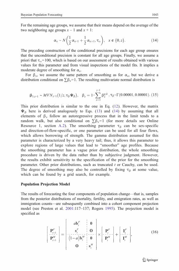
The data used to produce our forecasts represent the period 1975–2009. The data onmortality rates were obtained from the Human Mortality Database (n.d.). The emigra-tion and immigration counts were obtained from the Office for National Statistics. Thedata on births were obtained from the Office for National Statistics (England andWales), Northern Ireland Statistics Research Agency, and National Records ofScotland. The UK midyear population estimate for 2009, used as a baseline forpredictions, was also obtained from the Office for National Statistics. Logarithms ofsingle year mortality rates for females and males from 1975 to 2009 are presented in theupper row of Fig. 1. We observe that (1) mortality at all ages, and for both sexes, havebeen decreasing over time; (2) females have lower mortality than males; and (3) malesexhibit considerably higher mortality in the young adult years.

Fertility rates by age of mother are presented in the bottom row of Fig. 1. Overtime, we observe a shift from a peak level of fertility at ages 23–26 in 1970 towardone at ages 29–33 years in 2009. The reasons for this shift are related to fertilitypostponement and a subsequent recuperation. Because of the relatively small countsfor very young and very old ages, the data on births were aggregated into age groupsunder 15 years and 45 years and older. To compute fertility rates, the same femalepopulation at risk that was used to calculate the age-specific mortality was applied,except for the age groups under 15 and 45 and older, for which the population at riskwas aggregated for ages 12–14 years and 45–50 years, respectively. Further, in ourillustration, an implicit assumption was made about fertility—namely, that the ratesfor boundary ages (i.e., under 15 years and 45 years and older) are applied to thepopulation aged 14 years and 45 years, respectively. However, because these rates arevery small, the overall effect is negligible.

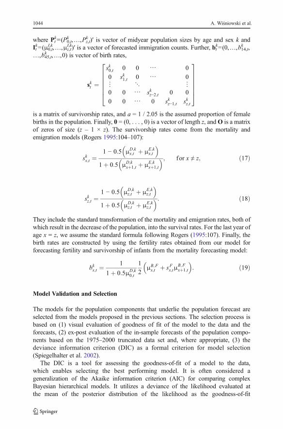
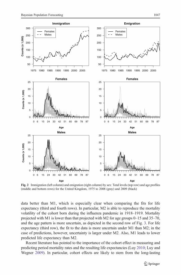
The total flows of immigration and emigration from 1975 to 2009 are presented inthe top row of Fig. 2. We observe similar trends in male and female migration overtime. The immigration levels increased rapidly from the 1990s through around 2005.For emigration, the increase is less noticeable and appears to be more volatile, whichmay be caused by random sample variation in the underlying data source, the


International Passenger Survey. Larger irregularities appear when the data are disag-gregated by single year of age, as illustrated for immigration and emigration in themiddle and bottom rows, respectively, of Fig. 2 (see also Raymer et al. 2011a).

Results

In this section, we present the results of forecasting the population components with themodels described in the previous section. For each component, we discuss the model’sgoodness-of-fit to the data and forecasts of the future patterns, and select the underlyingmodel to be used for the population forecast.

Forecasts of Mortality

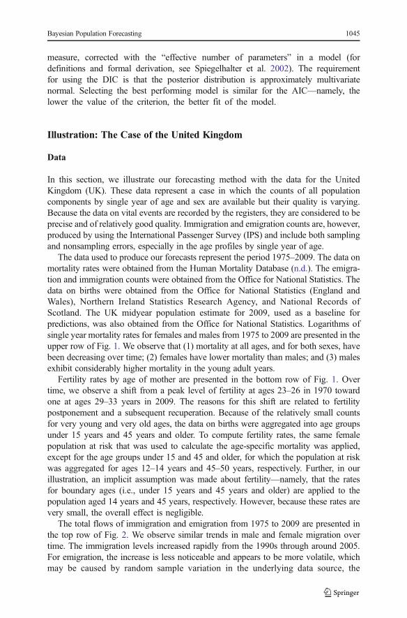
In the first row of Fig. 3, we present the fit of the models M1 and M2 to the 2009 data.It can be observed that the fit of the model M2 with the cohort component reflects the

−10

−8

−6

−4

−2

0Females

Age

Mo

rtal

ity

Rat

e (l

og

arit

hm

)

Mo

rtal

ity

Rat

e (l

og

arit

hm

)

0 9 18 27 36 45 54 63 72 81

−10

−8

−6

−4

−2

0Males

Age

0 9 18 27 36 45 54 63 72 81

0.00

0.02

0.04

0.06

0.08

0.10

0.12

0.14

Age

Fer

tilit

y R

ate

<15 17 20 23 26 29 32 35 38 41 44

Fig. 1 Logarithm of mortality rates by sex (top row) and fertility rates (bottom row) for the United Kingdom,1975 to 2008 (gray) and 2009 (black)


data better than M1, which is especially clear when comparing the fits for lifeexpectancy (third and fourth rows). In particular, M2 is able to reproduce the mortalityvolatility of the cohort born during the influenza pandemic in 1918–1919. Mortalityprojected with M1 is lower than that projected with M2 for age groups 0–15 and 35–70,and the age pattern is more uncertain, as depicted in the second row of Fig. 3. For lifeexpectancy (third row), the fit to the data is more uncertain under M1 than M2; in thecase of predictions, however, uncertainty is larger under M2. Also, M1 leads to lowerpredicted life expectancy than M2.

Recent literature has pointed to the importance of the cohort effect in measuring andpredicting period mortality rates and the resulting life expectancies (Luy 2010; Luy andWegner 2009). In particular, cohort effects are likely to stem from the long-lasting

50

100

150

200

250

300

ImmigrationC

ou

nts

(x

1,00

0)

1975 1980 1985 1990 1995 2000 2005

FemalesMales

50

100

150

200

250

300

Emigration

1975 1980 1985 1990 1995 2000 2005

FemalesMales

0

5

10

15

20

25Females

Age

Co

un

ts (

x 1,

000)

0 6 15 24 33 42 51 60 69 78 87

0

5

10

15

20

25Females

Age

0 6 15 24 33 42 51 60 69 78 87

0

5

10

15

20

25Males

Age

Co

un

ts (

x 1,

000)

0 6 15 24 33 42 51 60 69 78 87

0

5

10

15

20

25Males

Age

0 6 15 24 33 42 51 60 69 78 87

Fig. 2 Immigration (left column) and emigration (right column) by sex: Total levels (top row) and age profiles(middle and bottom rows) for the United Kingdom, 1975 to 2008 (gray) and 2009 (black)


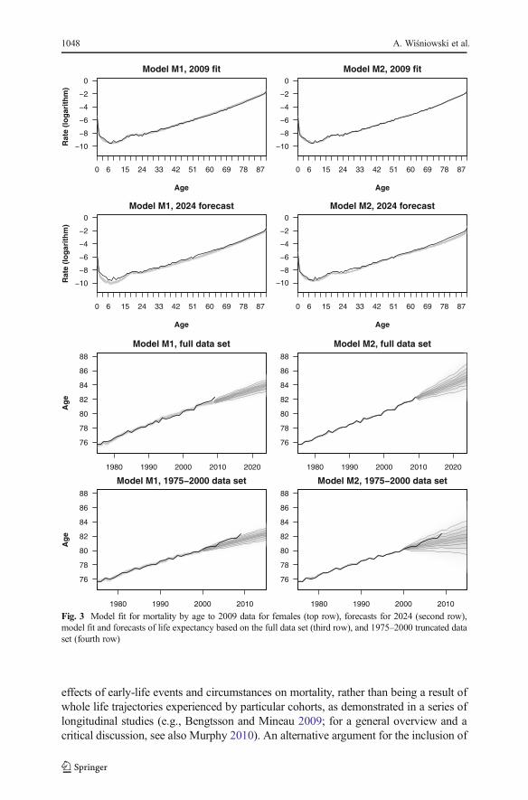
effects of early-life events and circumstances on mortality, rather than being a result ofwhole life trajectories experienced by particular cohorts, as demonstrated in a series oflongitudinal studies (e.g., Bengtsson and Mineau 2009; for a general overview and acritical discussion, see also Murphy 2010). An alternative argument for the inclusion of

−10

−8

−6

−4

−2

0

Model M1, 2009 fit

Age

Rat

e (l

og

arit

hm

)

0 6 15 24 33 42 51 60 69 78 87

−10

−8

−6

−4

−2

0

Model M2, 2009 fit

Age

0 6 15 24 33 42 51 60 69 78 87

−10

−8

−6

−4

−2

0

Model M1, 2024 forecast

Age

Rat

e (l

og

arit

hm

)

0 6 15 24 33 42 51 60 69 78 87

−8

−10

−6

−4

−2

0

Model M2, 2024 forecast

Age

0 6 15 24 33 42 51 60 69 78 87

1980 1990 2000 2010 2020

76

78

80

82

84

86

88

Model M1, full data set

Ag

e

1980 1990 2000 2010 2020

76

78

80

82

84

86

88

Model M2, full data set

1980 1990 2000 2010

76

78

80

82

84

86

88

Model M1, 1975−2000 data set

Ag

e

1980 1990 2000 2010

76

78

80

82

84

86

88

Model M2, 1975−2000 data set

Fig. 3 Model fit for mortality by age to 2009 data for females (top row), forecasts for 2024 (second row),model fit and forecasts of life expectancy based on the full data set (third row), and 1975–2000 truncated dataset (fourth row)


the cohort effect in the model is lifelong processes that might affect mortality, such assmoking (e.g., Doll et al. 2004).

To support our rationale for selecting model M2, we analyze the in-sample forecastsfrom both models based on the 1975–2000 truncated data set. Model M1 (the originalLee-Carter model) yields forecasts that slightly underpredict the observed life expec-tancy, which is presented in the bottom plot of Fig. 3. For M2, the posterior distributionis much wider than the results obtained with the full data set. Here, the medianpredictions seem to be slightly lower than the observed life expectancy, but theobserved values are inside the predictive intervals because of larger uncertainty. Acomparison of the ex-post forecasts reveals that 59 % of the observed mortality rates foryears 2001–2009 fall into the 80 % predictive intervals in the M1 model. For the 95 %predictive interval, 82 % of the observations fall into it. The M2 model performs better;the percentages of the observed mortality rates falling into 80 % and 95 % predictiveintervals are 75 % and 89 %, respectively. Because we model mortality rates in M1 anddeath counts in M2, the DIC cannot be used here to compare both models.

Our life expectancy forecasts can be compared with the official ones prepared by theOffice for National Statistics (2011). For 2024, the official predictions of 85.3 forfemales and 81.6 for males fall inside the 80 % predictive intervals. Median lifeexpectancies are 83.9 and 80.0 under M1, and 85.1 and 80.6 under M2. Hence, themodel with cohort effect (M2) leads to slightly lower predictions of life expectancycompared with the official ones, but higher predictions compared with M1.

Forecasts of Fertility

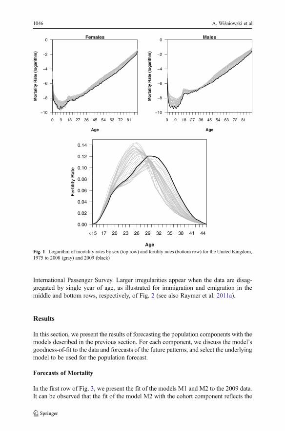
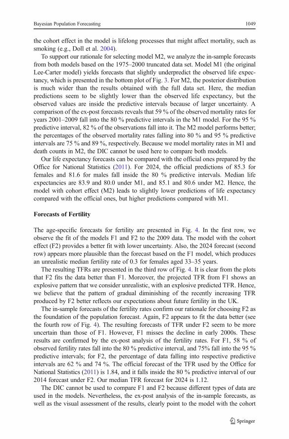
The age-specific forecasts for fertility are presented in Fig. 4. In the first row, weobserve the fit of the models F1 and F2 to the 2009 data. The model with the cohorteffect (F2) provides a better fit with lower uncertainty. Also, the 2024 forecast (secondrow) appears more plausible than the forecast based on the F1 model, which producesan unrealistic median fertility rate of 0.3 for females aged 33–35 years.

The resulting TFRs are presented in the third row of Fig. 4. It is clear from the plotsthat F2 fits the data better than F1. Moreover, the projected TFR from F1 shows anexplosive pattern that we consider unrealistic, with an explosive predicted TFR. Hence,we believe that the pattern of gradual diminishing of the recently increasing TFRproduced by F2 better reflects our expectations about future fertility in the UK.

The in-sample forecasts of the fertility rates confirm our rationale for choosing F2 asthe foundation of the population forecast. Again, F2 appears to fit the data better (seethe fourth row of Fig. 4). The resulting forecasts of TFR under F2 seem to be moreuncertain than those of F1. However, F1 misses the decline in early 2000s. Theseresults are confirmed by the ex-post analysis of the fertility rates. For F1, 58 % ofobserved fertility rates fall into the 80 % predictive interval, and 75% fall into the 95 %predictive intervals; for F2, the percentage of data falling into respective predictiveintervals are 62 % and 74 %. The official forecast of the TFR used by the Office forNational Statistics (2011) is 1.84, and it falls inside the 80 % predictive interval of our2014 forecast under F2. Our median TFR forecast for 2024 is 1.12.

The DIC cannot be used to compare F1 and F2 because different types of data areused in the models. Nevertheless, the ex-post analysis of the in-sample forecasts, aswell as the visual assessment of the results, clearly point to the model with the cohort


effect included. This rationale is supported by the vast demographic literature on thequantum and tempo effects in fertility (Bongaarts and Feeney 1998). In particular, werefer to the recent postponement and subsequent recuperation of fertility in manydeveloped countries, where the cohort effects are the most profound (see, e.g.,Sobotka et al. 2011). In our results, slightly declining but still uncertain fertility ratesmay indicate a possibility of yet another period of postponement.

0.0

0.1

0.2

0.3

0.4Model F1, 2009 fit

Age

Rat

e

14 17 20 23 26 29 32 35 38 41 44

0.0

0.1

0.2

0.3

0.4Model F2, 2009 fit

Age

14 17 20 23 26 29 32 35 38 41 44

0.0

0.1

0.2

0.3

0.4Model F1, 2024 forecast

Age

Rat

e

14 17 20 23 26 29 32 35 38 41 44

0.0

0.1

0.2

0.3

0.4Model F2, 2024 forecast

Age

14 17 20 23 26 29 32 35 38 41 44

1980 1990 2000 2010 2020

1.6

1.8

2.0

2.2

2.4

2.6

2.8

3.0Model F1, full data set

Rat

e

1980 1990 2000 2010 2020

1.6

1.8

2.0

2.2

2.4

2.6

2.8

3.0Model F2, full data set

1980 1990 2000 2010

1.6

1.8

2.0

2.2

2.4

2.6

2.8

3.0Model F1, 1975−2000 data set

Rat

e

1980 1990 2000 2010

1.6

1.8

2.0

2.2

2.4

2.6

2.8

3.0Model F2, 1975−2000 data set

Fig. 4 Model fit for fertility by age to 2009 data (top row), forecasts for 2024 (second row), model fit andforecasts of TFR based on the full data set (third row), and 1975–2000 truncated data set (fourth row)


Forecasts of Emigration and Immigration

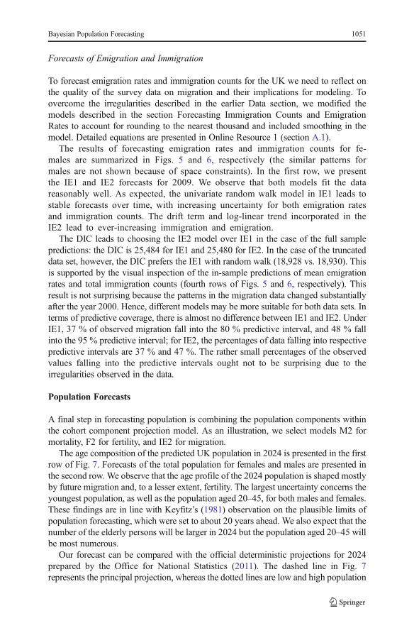
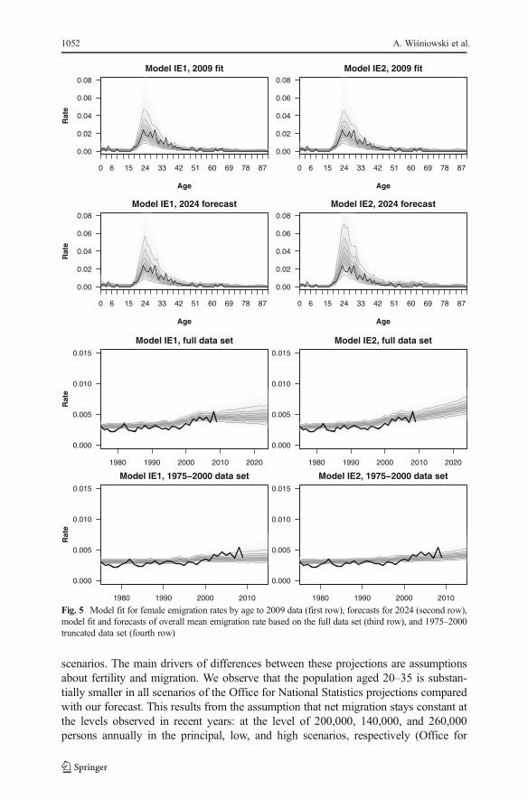
To forecast emigration rates and immigration counts for the UK we need to reflect onthe quality of the survey data on migration and their implications for modeling. Toovercome the irregularities described in the earlier Data section, we modified themodels described in the section Forecasting Immigration Counts and EmigrationRates to account for rounding to the nearest thousand and included smoothing in themodel. Detailed equations are presented in Online Resource 1 (section A.1).

The results of forecasting emigration rates and immigration counts for fe-males are summarized in Figs. 5 and 6, respectively (the similar patterns formales are not shown because of space constraints). In the first row, we presentthe IE1 and IE2 forecasts for 2009. We observe that both models fit the datareasonably well. As expected, the univariate random walk model in IE1 leads tostable forecasts over time, with increasing uncertainty for both emigration ratesand immigration counts. The drift term and log-linear trend incorporated in theIE2 lead to ever-increasing immigration and emigration.

The DIC leads to choosing the IE2 model over IE1 in the case of the full samplepredictions: the DIC is 25,484 for IE1 and 25,480 for IE2. In the case of the truncateddata set, however, the DIC prefers the IE1 with random walk (18,928 vs. 18,930). Thisis supported by the visual inspection of the in-sample predictions of mean emigrationrates and total immigration counts (fourth rows of Figs. 5 and 6, respectively). Thisresult is not surprising because the patterns in the migration data changed substantiallyafter the year 2000. Hence, different models may be more suitable for both data sets. Interms of predictive coverage, there is almost no difference between IE1 and IE2. UnderIE1, 37 % of observed migration fall into the 80 % predictive interval, and 48 % fallinto the 95 % predictive interval; for IE2, the percentages of data falling into respectivepredictive intervals are 37 % and 47 %. The rather small percentages of the observedvalues falling into the predictive intervals ought not to be surprising due to theirregularities observed in the data.

Population Forecasts

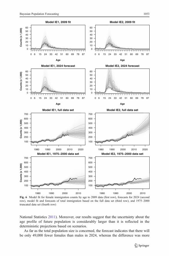
A final step in forecasting population is combining the population components withinthe cohort component projection model. As an illustration, we select models M2 formortality, F2 for fertility, and IE2 for migration.

The age composition of the predicted UK population in 2024 is presented in the firstrow of Fig. 7. Forecasts of the total population for females and males are presented inthe second row. We observe that the age profile of the 2024 population is shaped mostlyby future migration and, to a lesser extent, fertility. The largest uncertainty concerns theyoungest population, as well as the population aged 20–45, for both males and females.These findings are in line with Keyfitz’s (1981) observation on the plausible limits ofpopulation forecasting, which were set to about 20 years ahead. We also expect that thenumber of the elderly persons will be larger in 2024 but the population aged 20–45 willbe most numerous.

Our forecast can be compared with the official deterministic projections for 2024prepared by the Office for National Statistics (2011). The dashed line in Fig. 7represents the principal projection, whereas the dotted lines are low and high population


scenarios. The main drivers of differences between these projections are assumptionsabout fertility and migration. We observe that the population aged 20–35 is substan-tially smaller in all scenarios of the Office for National Statistics projections comparedwith our forecast. This results from the assumption that net migration stays constant atthe levels observed in recent years: at the level of 200,000, 140,000, and 260,000persons annually in the principal, low, and high scenarios, respectively (Office for

0.00

0.02

0.04

0.06

0.08

Model IE1, 2009 fit

Age

Rat

e

0 6 15 24 33 42 51 60 69 78 87

0.00

0.02

0.04

0.06

0.08

Model IE2, 2009 fit

Age

0 6 15 24 33 42 51 60 69 78 87

0.00

0.02

0.04

0.06

0.08

Model IE1, 2024 forecast

Age

Rat

e

0 6 15 24 33 42 51 60 69 78 87

0.00

0.02

0.04

0.06

0.08


Age

0 6 15 24 33 42 51 60 69 78 87

1980 1990 2000 2010 2020

0.000

0.005

0.010

0.015

Model IE1, full data set

Rat

e

1980 1990 2000 2010 2020

0.000

0.005

0.010

0.015


1980 1990 2000 2010

0.000

0.005

0.010

0.015

Model IE1, 1975−2000 data set

Rat

e

1980 1990 2000 2010

0.000

0.005

0.010

0.015


Fig. 5 Model fit for female emigration rates by age to 2009 data (first row), forecasts for 2024 (second row),model fit and forecasts of overall mean emigration rate based on the full data set (third row), and 1975–2000truncated data set (fourth row)


National Statistics 2011). Moreover, our results suggest that the uncertainty about theage profile of future population is considerably larger than it is reflected in thedeterministic projections based on scenarios.

As far as the total population size is concerned, the forecast indicates that there willbe only 49,000 fewer females than males in 2024, whereas the difference was more

0

10

20

30

40

50

60

Model IE1, 2009 fit

Age

Co

un

ts (

x 1,

000)

0 6 15 24 33 42 51 60 69 78 87

0

10

20

30

40

50

60

Model IE2, 2009 fit

Age

0 6 15 24 33 42 51 60 69 78 87

0

10

20

30

40

50

60


Age

Co

un

ts (

x 1,

000)

0 6 15 24 33 42 51 60 69 78 87

0

10

20

30

40

50

60


Age

0 6 15 24 33 42 51 60 69 78 87

1980 1990 2000 2010 2020

100

200

300

400

500

600

700


Co

un

ts (

x 1,

000)

1980 1990 2000 2010 2020

100

200

300

400

500

600

700


1980 1990 2000 2010

100

200

300

400

500

600

700


Co

un

ts (

x 1,

000)

1980 1990 2000 2010

100

200

300

400

500

600

700


Fig. 6 Model fit for female immigration counts by age to 2009 data (first row), forecasts for 2024 (secondrow), model fit and forecasts of total immigration based on the full data set (third row), and 1975–2000truncated data set (fourth row)


than 1 million in 2009 and was 1.5 million in favor of females in 1975. This is mostlikely due to the larger proportion of male migration and a gradual closing of the lifeexpectancy gap between the sexes. The median size of the 2024 population is 70.8million, which is around 9 million larger than the population size observed in 2009. Inthe principal projection for 2024 prepared by the Office for National Statistics (2011),the predicted total population is 69.0 million (i.e., 1.8 million lower), whereas the lowand high scenarios are 66.4 and 71.1 million, respectively. However, only high scenariofalls into our 80 % predictive interval for the total population. Also, the populationpredicted by the Office for National Statistics seems to be growing more slowly than inour forecast. This results from the aforementioned more-conservative prediction ofinternational net migration.

Males (left) Females (right)

Population Size (x 1,000)

Ag

e

0369

1215182124273033363942454851545760636669727578818487

90+

700 500 300 100 0 100 300 500 700

1980 1990 2000 2010 2020

Females

28,000

30,000

32,000

34,000

36,000

38,000

Po

pu

lati

on

Siz

e (x

1,0

00)

2024 Population

p25% = 34,738median = 35,336p75% = 35,984

1980 1990 2000 2010 2020

Males

Po

pu

lati

on

Siz

e (x

1,0

00)

28,000

30,000

32,000

34,000

36,000

38,0002024 Population

p25% = 34,708median = 35,385p75% = 36,174

1980 1990 2000 2010 2020

Total

Po

pu

lati

on

Siz

e (x

1,0

00)

60,000

65,000

70,000

2024 Population

p25% = 69,606median = 70,758p75% = 72,007

Fig. 7 2024 forecasts of males and females in the United Kingdom: Age profiles (first row) and totals (secondrow). Dashed lines are the 2010-based ONS principal projections with dotted lines representing the high andlow scenarios


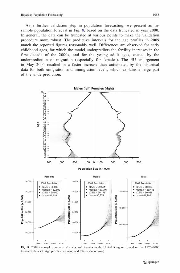
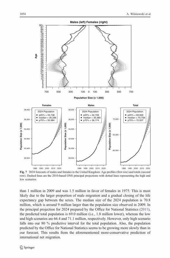
As a further validation step in population forecasting, we present an in-sample population forecast in Fig. 8, based on the data truncated in year 2000.In general, the data can be truncated at various points to make the validationprocedure more robust. The predictive intervals for the age profiles in 2009match the reported figures reasonably well. Differences are observed for earlychildhood ages, for which the model underpredicts the fertility increases in thefirst decade of the 2000s, and for the young adult ages, caused by theunderprediction of migration (especially for females). The EU enlargementin May 2004 resulted in a faster increase than anticipated by the historicaldata for both emigration and immigration levels, which explains a large partof the underprediction.

Males (left) Females (right)

Population Size (x 1,000)

Ag

e

0369

1215182124273033363942454851545760636669727578818487

90+

700 500 300 100 0 100 300 500 700

1980 1990 2000 2010

Females

28,000

30,000

32,000

34,000

36,000

38,000

Po

pu

lati

on

Siz

e (x

1,0

00)

2009 Population

p25% = 30,398median = 30,600p75% = 30,800data = 31,418

1980 1990 2000 2010

Males

28,000

30,000

32,000

34,000

36,000

38,000

Po

pu

lati

on

Siz

e (x

1,0

00)

2009 Population

p25% = 29,531median = 29,797p75% = 30,176data = 30,374

1980 1990 2000 2010

Total

60,000

65,000

70,000

Po

pu

lati

on

Siz

e (x

1,0

00)

2009 Population

p25% = 60,004median = 60,418p75% = 60,988data = 61,792

Fig. 8 2009 in-sample forecasts of males and females in the United Kingdom based on the 1975–2000truncated data set: Age profile (first row) and totals (second row)


Discussion

In this article, we have demonstrated that extension of the Lee-Carter model canserve as a general platform for estimating age schedules of the four demographiccomponents of population. We then combined these components into a singleforecast by means of a cohort-component projection model. We also explored thecorrelation of each of the components in time, as well as between sexes andcomponents (for emigration and immigration), which is embedded in our exten-sion of the Lee-Carter method. For emigration and immigration, we provided atool for smoothing irregularities in the data. This tool, however, can be easilyextended to fertility or mortality. Finally, we have illustrated the use of theforecasting model on the UK’s data.

This research makes two contributions to the literature. The first is the devel-opment of a new approach for integrating demographic components to providestochastic population forecasts by age and sex. The Bayesian approach that weadopted accounts for the uncertainties embedded in births, deaths, and emigrationand immigration, as well as across age and sexes. We show that the same generalframework of the Lee-Carter approach for modeling age and sex patterns ofmortality and fertility can be coherently applied to model corresponding patternsof migration. Irregularities in the data, such as those observed for the UK, can alsobe accounted for within the model.

The second contribution is the application of the approach to a situation of relativelygood yet imperfect data availability. In this way, we position our work between thegeneric global approach with far fewer data requirements, which has been proposed byRaftery et al. (2012), and a specific multiple-data situation discussed by Bryant andGraham (2013). Where possible, population forecasting should follow a bottom-upapproach, in which the age-specific rates of the demographic components are utilized.The rates describe the underlying processes more comprehensively than summaryaggregates, such as TFRs or life expectancies, in the top-down approach.

Further research should explore other models for forecasting age patterns of demograph-ic components, such as the functional models developed by Hyndman and Booth (2008).Analogously, various specifications for the time component models (such as ARIMA orVAR models of higher order) should be investigated. Next, the underlying models ofcomponents for the population forecast can be selected by using various techniques, ofwhich Bayesian model averaging (Raftery et al. 1997) seems to be most appealing. In thisway, the model uncertainty would be accounted for coherently. Finally, the uncertainty ofthe baseline population size used for projections could be incorporated into the projection.We believe this work provides a strong foundation for such extensions.

Acknowledgments We gratefully acknowledge a grant from the Economic and Social Research Council Centrefor Population Change (Grant RES-625-28-0001). We thank the Editor and four anonymous reviewers for theirvaluable comments and suggestions on this work; Jack Baker, Heather Booth, Jennifer M. Ortman, Adrian Rafteryand participants of the annual meeting of the Population Association of America 2013, New Orleans.

Open Access This article is distributed under the terms of the Creative Commons Attribution 4.0 InternationalLicense (http://creativecommons.org/licenses/by/4.0/), which permits unrestricted use, distribution, and repro-duction in any medium, provided you give appropriate credit to the original author(s) and the source, provide alink to the Creative Commons license, and indicate if changes were made.


References

Ahlburg, D. A., & Land, K. C. (Eds.). (1992). Population forecasting: Introduction. International Journal ofForecasting, 8, 289–299.

Alho, J. M. (1999, August). On probabilistic forecasts of population and their uses. Paper presented at the52nd Session of the International Statistical Institute, Helsinki, Finland.

Alho, J. M., & Spencer, B. D. (1985). Uncertain population forecasting. Journal of the American StatisticalAssociation, 80, 306–314.

Alho, J. M., & Spencer, B. D. (2005). Statistical demography and forecasting. New York, NY: Springer.Bengtsson, T., &Mineau, G. P. (2009). Early-life effects on socio-economic performance and mortality in later

life: A full life-course approach using contemporary and historical sources. Social Science & Medicine,68, 1561–1564.

Besag, J. E. (1986). On the statistical analysis of dirty pictures. Journal of the Royal Statistical Society: SeriesB, 48, 259–302.

Bijak, J. (2010). Forecasting international migration in Europe: A Bayesian view. Dordrecht,The Netherlands: Springer.

Bongaarts, J., & Bulatao, R. A. (Eds.). (2000). Beyond six billion: Forecasting the world’s population.Washington, DC: National Academy Press.

Bongaarts, J., & Feeney, G. (1998). When is a tempo effect a tempo distortion? Genus, 66, 1–15.Booth, H. (2006). Demographic forecasting: 1980 to 2005 in review. International Journal of Forecasting, 22,

547–581.Booth, H., & Tickle, L. (2008). Mortality modelling and forecasting: A review of methods. Annals of

Actuarial Science, 3, 3–43.Brass, W. (1974). Perspectives in population prediction: Illustrated by the statistics of England and Wales.

Journal of the Royal Statistical Society: Series A, 137, 532–570.Bryant, J. R., & Graham, P. J. (2013). Bayesian demographic accounts: Subnational population estimation

using multiple data sources. Bayesian Analysis, 8(2), 1–32.Cheng, P. C. R., & Lin, E. S. (2010). Completing incomplete cohort fertility schedules. Demographic

Research, 23(article 9), 223–256. doi:10.4054/DemRes.2010.23.9Coale, A., & Demeny, P. (1966). Regional model life tables and stable populations. Princeton, NJ: Princeton

University Press.Coale, A., & McNeil, D. R. (1972). The distribution by age of the frequency of first marriage in a female

cohort. Journal of the American Statistical Association, 67, 743–749.Coale, A., & Trussell, J. (1974). Model fertility schedules: Variations in the age structure of childbearing in

human populations. Population Index, 40, 185–258.Courgeau, D. (1985). Interaction between spatial mobility, family and career life-cycle: A French survey.

European Sociological Review, 1, 139–162.Czado, C., Delwarde, A., & Denuit, M. (2005). Bayesian Poisson log-bilinear mortality projections.

Insurance: Mathematics and Economics, 36, 260–284.Daponte, B., Kadane, J., & Wolfson, L. (1997). Bayesian demography: Projecting the Iraqi Kurdish popula-

tion, 1977–1990. Journal of the American Statistical Association, 92, 1256–1267.De Beer, J. (2011). A new relational method for smoothing and projecting age-specific fertility rates:

TOPALS. Demographic Research, 24(article 18), 409–454. doi:10.4054/DemRes.2011.24.18Doll, R., Peto, R., Boreham, J., & Sutherland, I. (2004). Mortality in relation to smoking: 50 years’

observations on male British doctors. British Medical Journal, 328, 1519. doi:10.1136/bmj.38142.554479.AE

Fienberg, S. E. (2013). Cohort analysis’ unholy quest: A discussion. Demography, 50, 1981–1984.Gelman, A. (2006). Prior distributions for variance parameters in hierarchical models. Bayesian Analysis, 1,

515–533.Girosi, F., & King, G. (2008). Demographic forecasting. Princeton, NJ: Princeton University Press.Heligman, L., & Pollard, J. H. (1980). The age pattern of mortality. Journal of the Institute of Actuaries, 107,

49–80.Human Mortality Database. (n.d.). University of California, Berkeley (USA), and Max Planck Institute for

Demographic Research (Germany). Retrieved from www.mortality.orgHyndman, R. J., & Booth, H. (2008). Stochastic population forecasts using functional data models for

mortality, fertility and migration. International Journal of Forecasting, 24, 323–342.Hyndman, R. J., & Ullah, M. S. (2007). Robust forecasting of mortality and fertility rates: A functional data

approach. Computational Statistics and Data Analysis, 51, 4942–4956.


http://dx.doi.org/10.4054/DemRes.2010.23.9

http://dx.doi.org/10.4054/DemRes.2011.24.18

http://dx.doi.org/10.1136/bmj.38142.554479.AE

http://dx.doi.org/10.1136/bmj.38142.554479.AE

http://www.mortality.org/

Hyppölä, J., Tunkelo, A., & Törnqvist, L. (1949). Suomen väestöä, sen uusiutumista ja tulevaa kehitystäkoskevia laskelmia [Calculations concerning the population of Finland, its renewal and future develop-ment] (Tilastollisia tiedonantoja, 38). Helsinki: Statistics Finland.

Keilman, N. (1990). Uncertainty in national population forecasting: Issues, backgrounds, analyses, recom-mendations. Amsterdam, The Netherlands: Swets & Zeitlinger.

Keyfitz, N. (1981). The limits of population forecasting. Population and Development Review, 7, 579–593.Knudsen, C., McNown, R., & Rogers, A. (1993). Forecasting fertility: An application of time series methods

to parameterized model schedules. Social Science Research, 22, 1–23.Lee, R. D. (1993). Modeling and forecasting the time series of US fertility: Age distribution, range, and

ultimate level. International Journal of Forecasting, 9, 187–202.Lee, R. D. (2000). The Lee-Carter method for forecasting mortality, with various extensions and applications.

North American Actuarial Journal, 4, 80–93.Lee, R. D., & Carter, L. R. (1992). Modelling and forecasting U.S. mortality. Journal of the American

Statistical Association, 87, 659–671.Lee, R. D., & Tuljapurkar, S. (1994). Stochastic population projections for the United States: Beyond high,

medium and low. Journal of the American Statistical Association, 89, 1175–1189.Li, N., & Lee, R. (2005). Coherent mortality forecasts for a group of populations: An extension of the Lee-

Carter method. Demography, 42, 575–594.Lunn, D., Spiegelhalter, D., Thomas, A., & Best, N. (2009). The BUGS project: Evolution, critique, and future

directions. Statistics in Medicine, 28, 3049–3067.Luo, L. (2013). Assessing validity and application scope of the intrinsic estimator approach to the age-period-

cohort problem. Demography, 50, 1945–1967.Lutz, W. (Ed.). (1996). The future population of the world: What can we assume today? London, UK:

Earthscan.Lutz, W., & Goldstein, J. R. (2004). Introduction: How to deal with uncertainty in population forecasting?

International Statistical Review, 72, 1–4.Luy, M. (2010). Tempo effects and their relevance in demographic analysis. Comparative Population Studies,

35, 415–446.Luy, M., & Wegner, C. H. (2009). Conventional versus tempo-adjusted life expectancy: Which is the more

appropriate measure for period mortality? Genus, 65, 1–28.McDonald, P., & Kippen, R. (2002). Projecting future migration levels: Should rates or numbers be used?

People and Place, 10, 82–83.Murphy, M. (2010). Reexamining the dominance of birth cohort effects on mortality. Population and

Development Review, 36, 365–390.Office for National Statistics. (2011). National Population Projections, 2010-based reference volume: Series

PP2. Titchfield, UK: Population Projections Unit, Office for National Statistics.Preston, S. H., Heuveline, P., & Guillot, M. (2001). Demography: Measuring and modeling population

processes. Oxford, UK: Blackwell.Raftery, A. E., Li, N., Ševcíková, H., Gerland, P., & Heilig, G. K. (2012). Bayesian probabilistic population

projections for all countries. Proceedings of the National Academy of Sciences of the USA, 109, 13915–13921.

Raftery, A. E., Madigan, D., & Hoeting, J. A. (1997). Bayesian model averaging for linear regression models.Journal of the American Statistical Association, 92, 179–191.

Raymer, J., Abel, G. J., Disney, G., & Wiśniowski, A. (2011a). Improving estimates of migration flows toEurostat (CPC Working Paper 15). Southampton, UK: ESRC Centre for Population Change, Universityof Southampton.

Raymer, J., De Beer, J., & Van der Erf, R. (2011b). Putting the pieces of the puzzle together: Age and sex-specific estimates of migration amongst countries in the EU/EFTA, 2002–2007. European Journal ofPopulation, 27, 185–215.

Rees, P. H. (1986). Choices in the construction of regional population projections. In R. I. Woods & P. H. Rees(Eds.), Population structures and models: Developments in spatial demography (pp. 126–159). London,UK: George Allen and Unwin.

Renshaw, A. E., & Haberman, S. (2006). A cohort-based extension to the Lee-Carter model for mortalityreduction factors. Insurance: Mathematics and Economics, 58, 556–570.

Rogers, A. (1986). Parameterized multistate population dynamics and projections. Journal of the AmericanStatistical Association, 81, 48–61.

Rogers, A. (1995). Multiregional demography: Principles, methods and extensions. Chichester, UK: JohnWiley & Sons.


Rogers, A., & Castro, L. J. (1981). Model migration schedules (Research Report 81-30). Laxenburg, Austria:International Institute for Applied Systems Analysis.

Rogers, A., & Little, J. S. (1994). Parameterizing age patterns of demographic rates with the multiexponentialmodel schedule. Mathematical Population Studies, 4, 175–195.

Rogers, A., Raquillet, R., & Castro, L. J. (1978). Model migration schedules and their applications.Environment and Planning A, 10, 475–502.

Smith, P. W. F., Raymer, J., & Giulietti, C. (2010). Combining available migration data in England to studyeconomic activity flows over time. Journal of the Royal Statistical Society: Series A, 173, 733–753.

Sobotka, T., Zeman, K., Lesthaeghe, R., Frejka, T., & Neels, K. (2011). Postponement and recuperation incohort fertility: Austria, Germany and Switzerland in a European context. Comparative PopulationStudies, 36, 417–452.

Spiegelhalter, D. J., Best, N. G., Carlin, B. P., & Van der Linde, A. (2002). Bayesian measures of modelcomplexity and fit. Journal of the Royal Statistical Society: Series B, 64, 585–639.

Wheldon, M. C., Raftery, A. E., Clark, S. J., & Gerland, P. (2013). Reconstructing past populations withuncertainty from fragmentary data. Journal of the American Statistical Association, 108, 96–110.

Wilson, T., & Bell, M. (2007). Probabilistic regional population forecasts: The example of Queensland,Australia. Geographical Analysis, 39, 1–25.


Documents

Bayesian Population Forecasting: Extending the Lee-Carter … · Bayesian Population Forecasting: Extending the Lee-Carter Method Arkadiusz Wiśniowski1 & PeterW.F.Smith1 & Jakub