Embed Size (px)
Citation preview

JSS Journal of Statistical SoftwareMMMMMM YYYY, Volume VV, Issue II. doi: 10.18637/jss.v000.i00
Bayesian random-effects meta-analysis
using the bayesmeta R package
Christian RoverUniversity Medical Center Gottingen
Abstract
The random-effects or normal-normal hierarchical model is commonly utilized in awide range of meta-analysis applications. A Bayesian approach to inference is very at-tractive in this context, especially when a meta-analysis is based only on few studies. Thebayesmeta R package provides readily accessible tools to perform Bayesian meta-analysesand generate plots and summaries, without having to worry about computational details.It allows for flexible prior specification and instant access to the resulting posterior distri-butions, including prediction and shrinkage estimation, and facilitating for example quicksensitivity checks. The present paper introduces the underlying theory and showcases itsusage.
Keywords: evidence synthesis, NNHM, between-study heterogeneity.
1. Introduction
1.1. Meta-analysis
Evidence commonly comes in separate bits, and not necessarily from a single experiment. Incontemporary science, the careful conduct of systematic reviews of the available evidence fromdiverse data sources is an effective and ubiquitously practiced means of compiling relevantinformation. In this context, meta-analyses allow for the formal, mathematical combinationof information to merge data from individual investigations to a joint result. Along withqualitative, often informal assessment and evaluation of the present evidence, meta-analyticmethods have become a powerful tool to guide objective decision-making (Chalmers et al.2002; Liberati et al. 2009; Hedges and Olkin 1985; Hartung et al. 2008; Borenstein et al. 2009).Applications of meta-analytic methods span such diverse fields as agriculture, astronomy,biology, ecology, education, health research, medicine, psychology, and many more (Chalmers
arX
iv:1
711.
0868
3v1
[st
at.C
O]
23
Nov
201
7
2 Meta-analysis using the bayesmeta package
et al. 2002).
When empirical data from separate experiments are to be combined, one usually needs tobe concerned about the straight one-to-one comparability of the provided results. Theremay be obvious or concealed sources of heterogeneity between different studies, originatinge.g. from differences in the selection and treatment of subjects, or in the exact definition ofoutcomes. Residual heterogeneity may be anticipated in the modeling stage and consideredin the estimation process; a common approach is to include an additional variance componentto account for between-study variability. On the technical side, the consideration of sucha heterogeneity parameter leads to a random-effects model rather than a fixed-effect model(Hedges and Olkin 1985; Hartung et al. 2008; Borenstein et al. 2009). Inclusion of a non-zeroheterogeneity will generally lead to more conservative results, and it may safeguard againstundesired Simpson’s paradox effects by explicitly stratifying the data before deriving a pooledestimate (Rucker and Schumacher 2008) rather than“naıvely”merging the given data withoutconsideration of potentially heterogeneous data sources.
1.2. The normal-normal hierarchical model (NNHM)
A wide range of problems may be approached using the normal-normal hierarchical model(NNHM); this generic random-effects model is applicable when the estimates to be combinedare given along with their uncertainties (standard errors) on a real-valued scale. Many prob-lems are commonly solved this way, often after a transformation stage to re-formulate theproblem on an appropriate scale. For example, binary data given in terms of contingencytables are routinely expressed in terms of logarithmic odds ratios (and associated standarderrors), which are then readily processed via the NNHM.
In the NNHM, measurements and standard errors are modeled via normal distributions,using means and their standard errors as sufficient statistics, while on a second hierarchylevel the heterogeneity is modeled as an additive normal variance component as well. Themodel then has two parameters, the (real-valued) effect, and the (positive) heterogeneity. Ifthe heterogeneity is zero, then the model reduces to the special case of a fixed-effect model(Hedges and Olkin 1985; Hartung et al. 2008; Higgins and Green 2011; Borenstein et al. 2009).The model and terminology are described in detail in Section 2.1 below.
The bayesmeta package is based on this simple yet ubiquitous form of the NNHM. A rangeof extensions or generalizations of the generic model are also commonly used, for exampleextending the focus to meta-regression or network meta-analysis, or refining the model toallow for uncertainty in standard errors, to discrete endpoints, or to non-normal heterogeneitycomponents. While the bayesmeta package focuses on a Bayesian approach to inference withinthe NNHM framework, frequentist approaches are implemented for R for example in themetafor and meta packages (Viechtbauer 2010; Schwarzer 2007; Schwarzer et al. 2015).
1.3. Analysis within the NNHM framework
The Bayesian solution
The bayesmeta package implements a Bayesian approach to inference. Bayesian modeling haspreviously been advocated and used in the meta-analysis context (Smith et al. 1995; Suttonand Abrams 2001; Spiegelhalter 2004; Spiegelhalter et al. 2004; Higgins et al. 2009; Lunn
Journal of Statistical Software 3
et al. 2013); the difference to the more common “frequentist” methods is that the problemis approached by expressing states of information via probability distributions, where theconsideration of new data then constitutes an update to a previous information state (Gelmanet al. 2014; Jaynes 2003; Spiegelhalter et al. 1999). A Bayesian analysis allows (and in factrequires) the specification of prior information, expressing the a priori knowledge, before dataare taken into account. Technically this means the definition of a probability distribution,the prior distribution, over the unknowns in the statistical model. Once model and prior arespecified, the results of a Bayesian analysis are uniquely determined; however, implementingthe necessary computations to derive these in practice may still be tricky.
While analysis results will of course depend on the prior specification, the range of reasonablespecifications however is usually limited. In the meta-analysis context, non-informative orweakly informative priors for the effect are readily defined, if required, while for the between-study heterogeneity an informative specification is often appropriate, especially when onlya small number of studies is involved. Interestingly, the number of studies combined in themeta-analyses archived in the Cochrane Library is reported by both Davey et al. (2011) andKontopantelis et al. (2013) with a median of 3 and a 75% quantile of 6, so that in practice amajority of analyses here is based on as few as 2–3 studies; such cases may be not as unusual asone might expect. Standard options are available here, confining the prior probability withinreasonable ranges (Spiegelhalter et al. 2004). Long-run properties of Bayesian methods havealso been compared with common frequentist approaches by Friede et al. (2017a,b), with afocus on the common case of very few studies.
Bayesian methods commonly are computationally more demanding than other methods; usu-ally these require the determination of high-dimensional integrals. In some (usually simpler)cases, the necessary integrals can be solved analytically, but it was mostly with the advent ofmodern computers and especially the development of Markov chain Monte Carlo (MCMC)methods that Bayesian analyses have become more generally tractable (Metropolis and Ulam1949; Gilks et al. 1996). In the present case of random-effects meta-analysis within theNNHM, where only two unkown parameters are to be inferred, computations may be simpli-fied by utilizing numerical integration or importance resampling (Turner et al. 2015), bothof which require relatively little manual tweaking in order to get them to work. It turns outthat computations may be done partly analytically and partly numerically, offering anotherapproach to simplify calculations via the direct algorithm (Rover and Friede 2017). Utiliz-ing this method, the bayesmeta package provides direct access to quasi-analytical posteriordistributions without having to worry about setup, diagnosis or post-processing of MCMCalgorithms. The present paper describes some of the methods along with the usage of thebayesmeta package.
Other common approaches
In the frequentist framework, meta-analysis using the NNHM is most commonly done in twostages, where first the heterogeneity parameter is estimated, and then the effect estimate isderived based on the heterogenity estimate. The choice of a heterogeneity estimator poses aproblem on its own; a host of different heterogeneity estimators have been described, for acomprehensive summary of the most common ones see e.g. Veroniki et al. (2016). A commonproblem with such estimators of the heterogeneity variance component is that they frequentlyturn out as zero, effectively resulting in a fixed-effect model, which is usually seen as an un-desirable feature. Within this context, Chung et al. (2013) proposed a penalized likelihood
4 Meta-analysis using the bayesmeta package
approach, utilizing a Gamma type “prior” penalty term in order to guarantee non-zero het-erogeneity estimates.
The treatment and estimation of heterogeneity in practice has been investigated e.g. by Pul-lenayegum (2011), Turner et al. (2012) and Kontopantelis et al. (2013). When looking at largenumbers of meta-analyses published by the Cochrane Collaboration, the majority (57%) ofheterogeneity estimates in fact turned out as zero (Turner et al. 2012), while the numbers arehigher for “small” meta-analyses, and lower for analyses involving many studies (Kontopan-telis et al. 2013). Meanwhile the choice of analysis method (fixed- or random-effects) alsocorrelates with the number of studies involved, with larger numbers of studies increasing thechances of a random-effects model being employed (Kontopantelis et al. 2013). Kontopanteliset al. (2013) also compared the fraction of heterogeneity estimates resulting as zero in actualmeta-analyses with that obtained from simulation, suggesting that heterogeneity is commonlyunderestimated or remains undetected.
Once an estimate for the amount of heterogeneity has been arrived at, what is commonlydone is to use this as a plug-in estimate and proceed to compute further tests and estimatesconditioning on the heterogeneity estimate as if its true value were known (Hedges and Olkin1985; Hartung et al. 2008; Borenstein et al. 2009). Such a procedure would be warranted if theheterogeneity estimate was estimated with relatively great precision. Notable exceptions hereare the methods proposed by Follmann and Proschan (1999); Hartung and Knapp (2001a,b)and Sidik and Jonkman (2002), where the estimation uncertainty in heterogeneity is accountedfor (on the technical side resulting in an inflated standard error and a heavier-tailed Student-tdistribution to be utilized for deriving tests or confidence intervals), or parameter estimationin the generalized inference framework (Friedrich and Knapp 2013).
In some statistical applications, there is little difference between the results from frequentistand Bayesian analyses; often one may be considered a limiting case of the other, while in-terpretations may still be somewhat different (Lindley 1977; Jaynes 1976; Spiegelhalter et al.1999). This is not necessarily the case in the present context, as meta-analyses are quitecommonly based on few studies, so that certain large-sample asymptotics may not apply. Acommon misconception, namely that a Bayesian analysis based on a uniform prior generallyyielded identical results to a frequentist, purely likelihood-based analysis, is exposed as suchhere. A crucial feature of meta-analysis problems is that one of the parameters, the het-erogeneity, is confined to a bounded parameter space, which sometimes causes problems forfrequentist methods (Mandelkern 2002), partly because heterogeneity estimates commonlyare not adequately characterized through a mere point estimate and an associated standarderror. The common use of a plug-in estimate for the heterogeneity in frequentist proceduresthen turns out problematic, as such a strategy usually only makes sense when the estimatedparameter is clearly bounded away from zero and associated with relatively little uncertainty.Within a Bayesian context, these issues do not pose difficulties, and inference on some pa-rameters while accounting for uncertainty in other nuisance parameters is straightforwardlysolved through marginalization.
1.4. Outline
The remaining paper is mostly arranged in two major parts. In the following Section 2, theunderlying theory is introduced; first the common NNHM (random-effects) model and itsnotation are explained, and prior distributions for the two parameters are discussed. Then

Journal of Statistical Software 5
the resulting likelihood, marginal likelihood and posterior distributions are presented andsome general points are introduced.
In Section 3, the actual usage of the bayesmeta package is demonstrated; an example data setis introduced, along which the steps of a Bayesian meta-analysis are shown. The determinationof summary statistics and plots, as well as possible variations in the analysis setup and thecomputation of posterior predictive p-values are exhibited. Section 4 then concludes with asummary.
2. Random-effects meta-analysis
2.1. The normal-normal hierarchical model
The aim is to infer a quantity µ, the effect, based on a number k of different measurementswhich are provided along with their corresponding uncertainties. What is known are the em-pirical estimates yi (of µ) that are associated with known standard errors σi; these constitutethe “input data”. The ith study’s measurement yi (where i = 1, . . . , k) is assumed to arise asexchangeable and normally distributed around the study’s true parameter value θi:
yi|θi, σi ∼ N(θi, σ2i ), (1)
where the variability is due to the sampling error, whose magnitude is given by the (known)standard error σi. All studies do not necessarily have identical true values θi; in order to ac-commodate potential between-study heterogeneity in the model, we assume that each study imeasures a quantity θi that differs from the overall mean µ by another exchangeable, normallydistributed offset with variance τ2 ≥ 0:
θi|µ, τ ∼ N(µ, τ2). (2)
This second model stage implements the random effects assumption.
Especially when the study-specific parameters θi are not of primary interest, the notationmay be simplified by integrating out the “intermediate” θi terms and stating the model in itsmarginal form as
yi|µ, τ, σi ∼ N(µ, σ2i + τ2) (3)
(Hedges and Olkin 1985; Hartung et al. 2008; Borenstein et al. 2009). The two unknownsremaining to be inferred are the mean effect µ and the heterogeneity τ , which is commonlyconsidered a nuisance parameter. The studies’ shrinkage estimates of θi are however some-times also of interest and may be inferred from the model as well. In the special case of zeroheterogeneity (τ = 0), the model simplifies to a fixed-effect model in which the study-specificmeans θi are all equal (θ1 = . . . = θk = µ).
Such two-stage hierarchical models of an overall mean (µ) and study-specific parameters (θi)with a random effect for each study are commonly utilized in meta-analysis applications.The simple case of normally distributed error terms at both stages is often convenient andeasily tractable, and it also constitutes a good approximation in many cases. So, while theeffect here is treated as a continuous parameter, the model is quite commonly utilized toalso process different types of data (e.g. logarithmic odds ratios from dichotomous data, etc.)
6 Meta-analysis using the bayesmeta package
after transformation to a real-valued effect scale (Hedges and Olkin 1985; Hartung et al. 2008;Borenstein et al. 2009; Viechtbauer 2010; Higgins and Green 2011).
2.2. Prior distributions
General
Among the two unknowns, the effect µ is commonly of primary interest, while the hetero-geneity τ usually is considered a nuisance parameter. In order to infer the parameters, weneed to specify our prior information about µ and τ in terms of their joint prior probabilitydensity function p(µ, τ). What exactly constitutes a reasonable prior distribution always de-pends on the given context (Gelman et al. 2014; Spiegelhalter et al. 2004; Jaynes 2003). Forcomputational convenience, in the following we assume that we can factor the prior densityinto independent marginals: p(µ, τ) = p(µ) × p(τ). While this may not seem unreasonable,depending on the context, one may also argue in favour of a dependent prior specification(e.g., Senn 2007; Pullenayegum 2011). In the following, we aim to provide a comprehensiveoverview of popular or sensible options. We will discuss proper as well as improper priors;when using improper priors, the usual care must be taken, as the resulting posterior thenmay or may not be a proper probability distribution (Gelman et al. 2014). The discussedheterogeneity priors are also summarized in Table 1 below.
The effect parameter µ
An obvious choice of a non-informative prior for the effect µ, being a location parameter, isan improper uniform distribution over the real line (Gelman et al. 2014; Spiegelhalter et al.2004; Jaynes 2003). A normal prior (with mean µp and variance σ2p) is a natural choice as aninformative prior for the effect µ, and these two are also the cases we will restrict ourselvesto for computational convenience and feasibility in the following. The normal prior hereconstitutes the conditionally conjugate prior distribution for the effect (see also Section 2.5below). The uninformative uniform prior would also result as the limiting case for increasingprior uncertainty (σp →∞).
A way to guide the choice of a vague prior is by consideration of unit information priors(Kass and Wasserman 1995). The idea here is to specify the prior such that its informationcontent (variance) is in some way, possibly somewhat heuristically, equivalent to a singleobservational unit. For example, if the endpoint is a logarithmic odds ratio (log-OR), aneutral unit information prior may be given by a normal prior with zero mean (centeredaround an odds ratio of 1, i.e., “no effect”) and a standard deviation of σp = 4. For aderivation, see also Appendix A.1.
The heterogeneity parameter τ : proper, informative priors
Especially since in the meta-analysis context one is commonly dealing with very small numbersof studies k, where not much information on between-study heterogeneity may be expectedto be gained from the data, it may be worth while considering the use of informative priors.Depending on the exact context, there often is some information on what values for theheterogeneity are more plausible and which ones are less so, and making use of the presentinformation may make a difference in the end. For example, if the meta-analysis is based on

Journal of Statistical Software 7
logarithmic odds ratios, it will usually make sense to assume that heterogeneity is unlikelyto exceed, say, τ = log(10)≈ 2.3, which would correspond to roughly an expected factor 10difference in effects (odds ratios) between trials due to heterogeneity. An extensive discussionof such cases is provided in Spiegelhalter et al. (2004, Sec. 5.7). Values for τ between 0.1 and0.5 here are considered “reasonable”, values between 0.5 and 1.0 are “fairly high” and valuesbeyond 1.0 are “fairly extreme”. An analogous reasoning would apply for similarly definedoutcomes, for example, logarithmic relative risks, logarithmic hazard ratios, or logarithmicvariances (Schmidli et al. 2017). Consideration of the magnitude of unit information variances(see previous paragraph) may also be helpful in this context, as variability (heterogeneity)between studies will usually be expected to be substantially below the variability betweenindividuals. Along these lines, it is often useful to also consider the implications of priorspecifications in terms of the corresponding prior predictive distributions; see also Section 3.4below. The impact of variations of how exactly prior information is implemented in the modelmay eventually also be checked via sensitivity analyses.
A sensible informative choice for p(τ) may be the maximum entropy prior for a pre-specifiedprior expectation E[τ ], the exponential distribution with rate λ = 1
E[τ ] (Jaynes 1968, 2003;
Gregory 2005). Log-normal or half-normal prior distributions, e.g. with pre-specified quan-tiles, may also be useful alternatives. For example, for log-OR (or similar) endpoints, theroutine use of half-normal distributions with scale 0.5 or 1.0 has been suggested by Friedeet al. (2017a,b) and was shown to work well in simulations. In order to gain robustness, onemay also consider mixture distributions as informative priors, for example half-Student-t, half-Cauchy, or Lomax distributions, which may be considered heavy-tailed variants of half-normalor exponential distributions (Johnson et al. 1994). Use of a heavy-tailed prior distributionwill allow for discounting of the prior in favour of the data in case the data appear to be inconflict with prior expectations (O’Hagan and Pericchi 2012; Schmidli et al. 2014). The use ofweakly informative half-Student-t or half-Cauchy priors may also be motivated via theoreticalarguments, as these can be shown to also exhibit favourable frequentist properties (Gelman2006; Polson and Scott 2012).
Although an inverse-Gamma distribution for an informative prior may seem to be an obviouschoice, use of this distribution is generally not recommended (Gelman 2006; Polson and Scott2012). More on informative (as well as uninformative) priors may be found in Spiegelhalteret al. (2004), Gelman (2006) and Polson and Scott (2012). Some empirical evidence to considerfor informative priors for certain types of endpoints may be found e.g. in Pullenayegum (2011),Turner et al. (2012) and Kontopantelis et al. (2013). In particular, Rhodes et al. (2015) andTurner et al. (2015) derived empirical priors based on data from the Cochrane database ofsystematic reviews; prior information here is expressed in terms of log-normal or log-Student-tdistributions.
The heterogeneity parameter τ : proper, ‘non-informative’ priors
Some “non-informative” proper priors have been proposed that are scale-invariant in the sensethat (like the Jeffreys prior discussed below as well) they depend only on the standard errors σi.A re-expression of the estimation problem on a different measurement scale would entail aproportional re-scaling of standard errors and so inference effectively remains unaffected.Such priors are discussed e.g. by Spiegelhalter et al. (2004, Sec. 5.7.3) and Berger and Deely(1988). Priors like these, however, are somewhat problematic from a logical perspective, asthese imply that the prior information on the heterogeneity depended on the accuracy of the
8 Meta-analysis using the bayesmeta package
individual studies’ estimates (Senn 2007).
The following two priors both depend on the harmonic mean s20 of squared standard errors,i.e.,
s20 =k∑k
i=1 σ−2i
. (4)
The uniform shrinkage prior results from considering the “average shrinkage” S(τ) =s20
s20+τ2 ;
placing a uniform prior on S(τ) results in a prior density
p(τ) =2τs20
(s20 + τ2)2(5)
for the heterogeneity, which has a median of s0. For a detailed discussion see e.g. Spiegelhalteret al. (2004) or Daniels (1999). A uniform prior in S(τ) is equivalent to a uniform prior
in 1−S(τ) = τ2
s20+τ2 (Spiegelhalter et al. 2004), which is an expression very similar to the
I2 measure of heterogeneity due to Higgins and Thompson (2002). Substiting the harmonicmean s20 for their average (s2) in the prior density (5) hence yields a uniform prior in I2.
The DuMouchel prior has a similar form and is defined through
p(τ) =s0
(s0 + τ)2. (6)
This implies a log-logistic distribution for the heterogeneity τ that has its mode at τ = 0 andits median at τ = s0 (Spiegelhalter et al. 2004; DuMouchel and Normand 2000).
A conventional prior as a proper variation of the Jeffreys prior (see also the closely relatedvariant in (12) below) was given by Berger and Deely (1988) as
p(τ) ∝k∏i=1
(τ
(σ2i + τ2)3/2
)1/k
. (7)
This prior is in particular intended as a non-informative but proper choice for testing or modelselection purposes (Berger and Deely 1988; Berger and Pericchi 2001).
The heterogeneity parameter τ : improper priors
Uninformative priors It is not so obvious what exactly would qualify a prior for τ as“uninformative”. One might argue that an uninformative prior should have a probabilitydensity function that is monotonically decreasing in τ ; another question would be whetherthe density’s intercept p(τ = 0) should be positive or finite, or what the density’s derivativenear zero should be. In general, the uninformative prior for a scale parameter in a simplenormal model is commonly taken to be uniform on log(τ) (and log(τ2)) with density p(τ) ∝ 1
τ(Jeffreys 1946; Gelman et al. 2014), however, this “log-uniform” prior will not lead to proper,integrable posteriors in the present context (Gelman 2006). Another reasonable choice maybe the improper uniform prior on the positive real line, but care must be taken here as usual,as the posterior may end up improper as well; this will not result in a proper posterior whenthere are only one or two estimates available (i.e., when k ≤ 2) and an (improper) uniformeffect prior is used (Gelman 2006). The uniform prior may be considered a conservative

Journal of Statistical Software 9
choice in a particular sense, as shown below (Appendix A.2), but on the other hand it mayalso be considered overly conservative, as it tends to attach a lot of weight to potentiallyunreasonably large heterogeneity values. Gelman (2006) generally recommends a uniformheterogeneity prior as an uninformative default, unless the number of studies k is small, oran informative prior is desired or for other reasons.
One may also argue via certain requirements that an uninformative prior should meet (Jaynes1968, 2003). For example, it may be reasonable to demand invariance with respect to re-scalingof τ for the prior density p(τ), leading to a constraint of the form
1s p(
τs ) = f(s) p(τ) (8)
for any scaling factor s > 0 and some positive-valued function f(s) (i.e., re-scaling should notaffect the density’s shape). This requirement obviously restricts the range of priors to thosewith monotonic density functions. It leads to a family of improper prior distributions withdensities
p(τ) ∝ τa (9)
for a ∈ R. This family includes (for a = −1) the common log-uniform prior for a scaleparameter mentioned above, or (for a = 0) the uniform prior. But this class also includesother interesting cases, like, for −1 < a < 0, a compromise between the above two uniformand log-uniform priors that is (locally) integrable over any interval [0, u] with 0 < u < ∞while also being shorter-tailed on the right than the improper uniform prior. An obviousexample is (for a = −0.5) the prior with monotonically decreasing density function
p(τ) ∝ 1√τ
(10)
which corresponds to a uniform prior in√τ . This prior has the unusual property that the
prior density, and with that the posterior as well, exhibits a pole (i.e., approaches infinity) atthe origin. A value of a=1 would lead to a uniform prior in τ2, with an even higher preferencefor large heterogeneity values, which requires at least k≥4 studies for a proper posterior; thisprior is generally not recommended (Gelman 2006).
The Jeffreys prior The non-informative Jeffreys prior (Gelman et al. 2014; Jeffreys 1946)for this problem results from the form of the likelihood (see equation (3) or (14) below), ormore specifically, the associated expected Fisher information J(µ, τ); its probability density
function is given by p(µ, τ) ∝√
det(J(µ, τ)). This general form of Jeffreys’ prior however isgenerally not recommended when the set of parameters includes a location parameter as in thepresent case; see e.g. Jeffreys (1946), Jeffreys (1961, Sec. III.3.10), Berger (1985, Sec. 3.3.3)and Kass and Wasserman (1996, Sec. 2.2). Instead, location parameters are commonly treatedas fixed and are conditioned upon (Berger 1985; Kass and Wasserman 1996). In the presentcase (since µ and τ are orthogonal in the sense that the Fisher information matrix’ off-diagonalelements are zero), this leads to Tibshirani’s non-informative prior (Tibshirani 1989; Kass andWasserman 1996, Sec. 3.7), a variation of the general Jeffreys prior, which is of the form
p(τ) ∝
√√√√ k∑i=1
( τ
σ2i + τ2
)2. (11)
10 Meta-analysis using the bayesmeta package
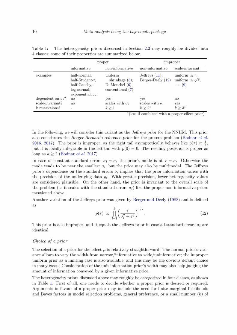
Table 1: The heterogeneity priors discussed in Section 2.2 may roughly be divided into4 classes; some of their properties are summarized below.
proper improper
informative non-informative non-informative scale-invariant
examples half-normal,half-Student-t,half-Cauchy,log-normal,exponential, . . .
uniformshrinkage (5),
DuMouchel (6),conventional (7)
Jeffreys (11),Berger-Deely (12)
uniform in τ ,uniform in
√τ ,
. . . (9)
dependent on σi? no yes yes noscale-invariant? no scales with σi scales with σi yesk restrictions? - k ≥ 1 k ≥ 2∗ k ≥ 3∗
∗(less if combined with a proper effect prior)
In the following, we will consider this variant as the Jeffreys prior for the NNHM. This prioralso constitutes the Berger-Bernardo reference prior for the present problem (Bodnar et al.2016, 2017). The prior is improper, as the right tail asymptotically behaves like p(τ) ∝ 1
τ ,but it is locally integrable in the left tail with p(0) = 0. The resuling posterior is proper aslong as k ≥ 2 (Bodnar et al. 2017).
In case of constant standard errors σi = σ, the prior’s mode is at τ = σ. Otherwise themode tends to be near the smallest σi, but the prior may also be multimodal. The Jeffreysprior’s dependence on the standard errors σi implies that the prior information varies withthe precision of the underlying data yi. With greater precision, lower heterogeneity valuesare considered plausible. On the other hand, the prior is invariant to the overall scale ofthe problem (as it scales with the standard errors σi) like the proper non-informative priorsmentioned above.
Another variation of the Jeffreys prior was given by Berger and Deely (1988) and is definedas
p(τ) ∝k∏i=1
(τ
σ2i + τ2
)1/k
. (12)
This prior is also improper, and it equals the Jeffreys prior in case all standard errors σi areidentical.
Choice of a prior
The selection of a prior for the effect µ is relatively straightforward. The normal prior’s vari-ance allows to vary the width from narrow/informative to wide/uninformative; the improperuniform prior as a limiting case is also available, and this may be the obvious default choicein many cases. Consideration of the unit information prior’s width may also help judging theamount of information conveyed by a given informative prior.
The heterogeneity priors discussed above may roughly be categorized in four classes, as shownin Table 1. First of all, one needs to decide whether a proper prior is desired or required.Arguments in favour of a proper prior may include the need for finite marginal likelihoodsand Bayes factors in model selection problems, general preference, or a small number (k) of
Journal of Statistical Software 11
τ
p(τ)
s0
0.0 0.5 1.0 1.5 2.0
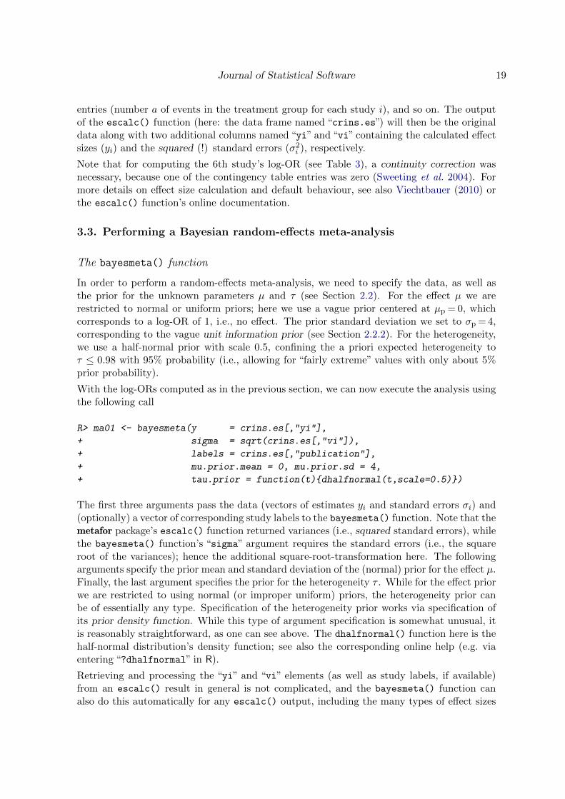
half−normal(0.5)half−Cauchy(0.5)log−normal(−1.07, 0.87)uniform shrinkageDuMouchelconventionalJeffreysBerger−Deely
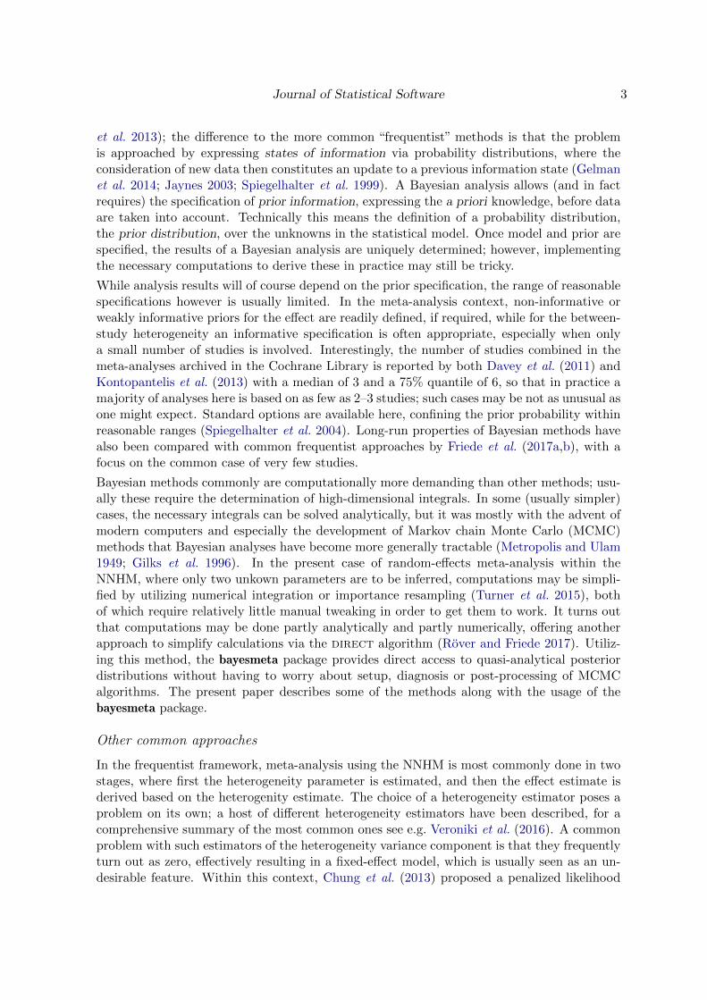
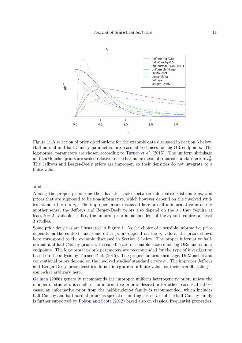
Figure 1: A selection of prior distributions for the example data discussed in Section 3 below.Half-normal and half-Cauchy parameters are reasonable choices for log-OR endpoints. Thelog-normal parameters are chosen according to Turner et al. (2015). The uniform shrinkageand DuMouchel priors are scaled relative to the harmonic mean of squared standard errors s20.The Jeffreys and Berger-Deely priors are improper, so their densities do not integrate to afinite value.
studies.
Among the proper priors one then has the choice between informative distributions, andpriors that are supposed to be non-informative, which however depend on the involved stud-ies’ standard errors σi. The improper priors discussed here are all uninformative in one oranother sense; the Jeffreys and Berger-Deely priors also depend on the σi, they require atleast k = 2 available studies, the uniform prior is independent of the σi and requires at least3 studies.
Some prior densities are illustrated in Figure 1. As the choice of a sensible informative priordepends on the context, and some other priors depend on the σi values, the priors shownhere correspond to the example discussed in Section 3 below. The proper informative half-normal and half-Cauchy priors with scale 0.5 are reasonable choices for log-ORs and similarendpoints. The log-normal prior’s parameters are recommended for the type of investigationbased on the anlysis by Turner et al. (2015). The proper uniform shrinkage, DuMouchel andconventional priors depend on the involved studies’ standard errors σi. The improper Jeffreysand Berger-Deely prior densities do not integrate to a finite value, so their overall scaling issomewhat arbitrary here.
Gelman (2006) generally recommends the improper uniform heterogeneity prior, unless thenumber of studies k is small, or an informative prior is desired or for other reasons. In thosecases, an informative prior from the half-Student-t family is recommended, which includeshalf-Cauchy and half-normal priors as special or limiting cases. Use of the half-Cauchy familyis further supported by Polson and Scott (2012) based also on classical frequentist properties.

12 Meta-analysis using the bayesmeta package
If, for example, the endpoint is a log-OR, then, using the categorization by Spiegelhalteret al. (2004, Sec. 5.7), a half-normal prior with scale 0.5 may confine heterogeneity mostlyto “reasonable” to “fairly high” values and leave about 5% probability for “fairly extreme”heterogeneity. A larger scale parameter or a heavier-tailed distribution may then serve asa more conservative or more robust reference for a sensitivity check (Friede et al. 2017a,b).The Jeffreys prior constitutes another default choice of an uninformative prior; as the Berger-Bernardo reference prior it represents the least informative prior in a certain sense (Bodnaret al. 2017), and it will yield a proper posterior as long as at least 2 studies are available.
2.3. Likelihood
The form of the likelihood follows from the assumptions introduced in Section 2.1. TheNNHM is essentially a simple normal model with unknown mean and an unknown variancecomponent; the resulting likelihood function is given by
p(~y|µ, τ, ~σ) = (2π)−k2 ×
k∏i=1
1√σ2i + τ2
exp
(−1
2
(yi − µ)2
σ2i + τ2
), (13)
where ~y and ~σ denote the vectors of k effect measures yi and their standard errors σi. Forany practical application it is often more useful to consider the logarithmic likelihood, i.e.,
log(p(~y|µ, τ, ~σ)) = −k2 log(2π)− 1
2
k∑i=1
(log(σ2i + τ2) +
(yi − µ)2
σ2i + τ2
). (14)
2.4. Marginal likelihood
Marginalization
In order to do inference within a Bayesian framework, it is usually necessary to computeintegrals involving the posterior distribution (Gelman et al. 2014). For example, in a multi-parameter model, one may be interested in the marginal posterior distribution or in theposterior expectation of a certain parameter, both of which result as integrals. Key to thebayesmeta implementation is the partly analytical and partly numerical integration over pa-rameter space. In the following, we will derive the marginal posterior distribution of theheterogeneity parameter via the marginal likelihood, and we will later see how marginal andconditional distributions may be utilized to evaluate the required integrals. The likelihoodis initially a function of both parameters (µ and τ), and the marginal likelihood of the het-erogeneity τ results from integration over the effect µ, using its prior distribution, which wespecified to be either uniform or normal.
Uniform prior
Using the improper uniform prior for the effect µ (p(µ) ∝ 1), we can derive the marginallikelihood, marginalized over µ,
p(~y|τ, ~σ) =
∫p(~y|µ, τ, ~σ) p(µ) dµ. (15)

Journal of Statistical Software 13
For the NNHM, the integral turns out as
p(~y|τ, ~σ) = (2π)−k−12 ×
k∏i=1
1√σ2i + τ2
× exp
(−1
2
(yi − µ(τ))2
σ2i + τ2
)× 1√∑k
i=11
σ2i +τ
2
, (16)
where µ(τ) is the conditional posterior mean of µ for a given heterogeneity τ . Conditionalmean and standard deviation are given by
µ(τ) = E[µ|τ, ~y, ~σ] =
∑ki=1
yiσ2i +τ
2∑ki=1
1σ2i +τ
2
and σ(τ) =√
Var(µ|τ, ~y, ~σ) =
√√√√ 1∑ki=1
1σ2i +τ
2
.
(17)A derivation is provided in Appendix A.3; the standard deviation σ(τ) will become relevantlater on. On the logarithmic scale the marginal likelihood then is:
log(p(~y|τ, ~σ))
= −1
2
((k−1) log(2π) +
k∑i=1
(log(σ2i +τ2) +
(yi − µ(τ))2
σ2i + τ2
)+ log
( k∑i=1
1
σ2i +τ2
)). (18)
Conjugate normal prior
The normal effect prior here is the conditionally conjugate prior distribution, since the result-ing conditional posterior (for a given τ value) again is of a normal form. Calculations for the(proper) normal prior for the effect µ work similarly to the previous derivation. Assume theprior for µ is normal with mean µp and variance σ2p, i.e., it is defined through the probabil-
ity density function p(µ) = 1√2π σp
exp(−12(µ−µp)2
σ2p
). The necessary integral for the marginal
likelihood then results as
p(~y|τ, ~σ) =
∫p(~y|µ, τ, ~σ) p(µ) dµ (19)
= (2π)−k+12 × 1√
σ2p×
k∏i=1
1√σ2i + τ2
×∫
exp
(−1
2
[(µ− µp)2
σ2p+
k∑i=1
(yi − µ)2
σ2i + τ2
])dµ. (20)
One can see that the prior parameters (µp and σp) enter in a similar manner as the datapoints (yi and σi). In analogy to the previous derivation, define the conditional posteriormean and standard deviation
µ(τ) =
µpσ2p
+∑ki=1
yiσ2i +τ
2
1σ2p
+∑ki=1
1σ2i +τ
2
and σ(τ) =1√
1σ2p
+∑ki=1
1σ2i +τ
2
, (21)
and the logarithmic marginal likelihood turns out as
log(p(~y|τ, ~σ)) = −1
2
(k log(2π) + log(σ2p) +
k∑i=1
log(σ2i +τ2)
+(µp − µ(τ))2
σ2p+
k∑i=1
(yi − µ(τ))2
σ2i + τ2+ log
(1
σ2p+
k∑i=1
1
σ2i +τ2
)).(22)

14 Meta-analysis using the bayesmeta package
Note that, comparing equations (18) and (22) (as well as (17) and (21)), as expected, use ofthe uniform prior constitutes the limiting case of large prior uncertainty (σp →∞).
2.5. Conditional effect posteriors
As long as a uniform or normal prior for the effect µ is used, the effect’s conditional posteriordistribution for a given heterogeneity value, p(µ|τ, ~y, ~σ), again is normal with mean µ(τ) andstandard deviation σ(τ) as given in equations (17) or (21), respectively (Gelman et al. 2014).
Note that the conditional posterior moments (17) are also commonly utilized in frequentistfixed-effect and random-effects meta-analyses. The mean µ(τ) constitutes the conditionalmaximum likelihood estimate (of µ), conditional on a particular amount of heterogeneity τ ,while σ(τ) gives the corresponding (conditional) standard error. Plugging in τ =0 yields thefixed-effect estimate of µ, while a value τ > 0 yields a random-effects estimate (Hedges andOlkin 1985, Sec. 6); see also Section 3.5 below for an example.
2.6. Marginal and joint posterior
Having derived the marginal likelihood p(~y|τ, ~σ) in Section 2.4, the (one-dimensional) margin-al posterior density of τ may be computed (up to a normalizing constant) by multiplicationwith the heterogeneity prior
p(τ |~y, ~σ) ∝ p(~y|τ, ~σ)× p(τ). (23)
This feature was one of the reasons for specifying the priors for µ and τ as independent (seeSection 2.2.1). One-dimensional integration can now easily be done numerically for arbitrarypriors p(τ), as long as the resulting posterior is proper.
The effect’s conditional posterior p(µ|τ, ~y, ~σ) (see Section 2.5) is of particular interest, sincethe joint posterior may be re-expressed in terms of the conditional as
p(µ, τ |~y, ~σ) = p(µ|τ, ~y, ~σ)× p(τ |~y, ~σ). (24)
In this formulation, it becomes obvious that the effect’s marginal distribution is a continuousmixture distribution, in which the normal conditionals p(µ|τ, ~y, ~σ) are mixed via the marginalp(τ |~y, ~σ) with
p(µ|~y, ~σ) =
∫p(µ, τ |~y, ~σ) dτ =
∫p(µ|τ, ~y, ~σ)× p(τ |~y, ~σ) dτ (25)
(Seidel 2010; Lindsay 1995). This expression allows for easy numerical approximation ofposterior integrals of interest. For example, the marginal distribution of the effect µ (thenormal mixture) may be approximated by using a discrete grid of τ values and summing upthe normal conditionals using weights defined through τ ’s marginal density:
p(µ) =
∫p(µ|τ) p(τ) dτ ≈
∑j
p(µ|τj)wj , (26)
where the set of τj is appropriately chosen and corresponding “weights”wj (with∑j wj = 1)
are based on the marginal p(τ). With that, it is now relatively straightforward to work withthe joint distribution, derive marginals, moments, implement Monte Carlo integration, and
Journal of Statistical Software 15
so on. A general prescription of how to approach a discrete approximation as sketched in(26) while keeping the accuracy under control is given by the direct algorithm describedby Rover and Friede (2017). A few more technical details are also given in Section 2.11 andAppendix A.4 below.
2.7. Predictive distribution
The predictive distribution expresses the posterior knowledge about a “future” observation,i.e., an additional draw θk+1 from the underlying population of studies. This is commonly ofinterest in order to judge the amount of heterogeneity relative to the estimation uncertainty(Riley et al. 2011; Guddat et al. 2012; Bender et al. 2014), or for extrapolation in the designand analysis of future studies (Schmidli et al. 2014). Technically, the predictive distributionp(θk+1|~y, ~σ) is similar to the marginal distribution of the effect µ (see previous section).Conditionally on a given heterogeneity τ , and for the uniform or normal effect prior, thepredictive distribution again is normal with moments
E[θk+1 | τ, ~y, ~σ] = µ(τ) and Var(θk+1 | τ, ~y, ~σ) = σ2(τ) + τ2. (27)
2.8. Shrinkage estimates of study-specific means
Sometimes it is of interest to also infer the posterior distributions of the study-specific pa-rameters θj . These may e.g. be in the focus if a meta-analysis is performed in order supportthe analysis of a particular study by borrowing strength from a number of related studies(Gelman et al. 2014; Schmidli et al. 2014; Wandel et al. 2017). Conditionally on a particularheterogeneity value τ , these distributions are again normal with moments given by
E[θj | τ, ~y, ~σ] =
1σ2jyj + 1
τ2µ(τ)
1σ2j
+ 1τ2
(28)
Var(θj | τ, ~y, ~σ) =1
1σ2j
+ 1τ2
+
(1τ2
1σ2j
+ 1τ2σ
)2
(29)
(Gelman et al. 2014, Sec. 5.5). These expressions illustrate the shrinkage of posterior estimatestowards the common mean as a function of the heterogeneity. Analogously to the effectposterior and predictive distribution, these conditional moments again allow to approximateeach individual θi’s (marginal) posterior distribution via a discrete mixture to marginalizeover the heterogeneity.
2.9. Credible intervals
Credible intervals derived from a posterior probability distribution may be computed e.g.using the distribution’s α
2 and (1−α2 ) quantiles. However, such a simple central interval may
not necessarily be the most sensible summary of a posterior distribution, especially if it isskewed or extends to the boundary of its parameter space. In such cases, it usually makesmore sense to consider the highest posterior density (HPD) region, i.e., a (1−α) credible regionenclosing the (1−α) posterior probability where the posterior density is largest (Gelman et al.2014). Such a region may be disjoint and hard to determine, but closely related (and identical

16 Meta-analysis using the bayesmeta package
for unimodal distributions) is the shortest credible interval. Both types of intervals, centraland shortest, will be considered in the following.
2.10. Posterior predictive checks and p-values
Posterior predictive model checks allow to investigate the fit of a model to a given data set(Gelman et al. 1996; Gelman 2003; Gelman et al. 2014). The consistency of data and modelis explored by comparing the actual data to data sets predicted via the posterior distribution.The comparison is usually done graphically, or via suitable summary statistics of actual andpredicted data; a discrepancy then is an indicator of a poor model fit.
If the summary statistic is one-dimensional, then the comparison may be formalized by fo-cusing on the fractions of predicted values above or below the actually observed value. Thisleads to the concept of posterior predictive p-values, which are closely related to classical p-values (Meng 1994; Berkhof et al. 2000; Gelman 2013; Wasserstein 2016). Posterior predictivep-values have been applied and advocated in a range of contexts, including e.g. educationaltesting (Sinharay et al. 2006), metrology (Kacker et al. 2008), psychology (van de Schootet al. 2014) and biology (Chambert et al. 2014).
In the context of the NNHM, posterior predictive checks are useful, as they allow to investigatecertain hypotheses of interest, like for example µ ≥ 0, τ = 0 or θi = 0. The posterior predictivedistribution conditional on a particular hypothesis may then be explored in order to derive acorresponding posterior predictive p-value. The choice of a suitable summary statistic howevermay still pose a challenge. The posterior predictive checks here are implemented via MonteCarlo sampling, therefore parts of these procedures are computationally expensive.
2.11. How the bayesmeta() function works internally
The bayesmeta() function utilizes the fact that in the context of the NNHM the resultingposterior is only 2-dimensional (for now ignoring the θi parameters) and may be expressed asa mixture distribution (see (24)) where the heterogeneity’s marginal p(τ |~y, ~σ) is known, andthe effect’s conditionals p(µ|τ, ~y, ~σ) are all of a normal form. This setup allows to approximatethe effect marginal by a discrete mixture (see (26)) while keeping the accuracy under control;the accuracy requirements are formulated via the direct algorithm’s two tuning parameters(δ and ε) (Rover and Friede 2017).
An example of joint and marginal posterior densities of the two parameters is illustratedin Figure 3 below (see page 22). The joint posterior density (top right) is easily evaluatedbased on likelihood and prior density, both of which are available in analytical form (seeSections 2.2 and 2.3). The heterogeneity’s marginal density (bottom right) is also easilycomputed, based on marginal likelihood and prior (see (23)); only its normalizing constantneeds to be computed numerically (using the integrate() function available in R). The CDFis also computed using numerical integration, and the quantile function is evaluated usingagain the CDF and inverting it via R’s uniroot() root-finding function.
Now the effect’s marginal density (bottom left panel of Figure 3) is approximated by a mixtureof a finite number of normal distributions. In terms of equation (26), what is required is a finiteset of support points τj , the parameters (means and standard deviations) of the associatednormal conditionals p(µ|τj), and the corresponding weights wj . These are all determinedusing the direct algorithm, and in the bayesmeta() output (see the following section) one
Journal of Statistical Software 17
can find these in the “...$support” element. In the example shown in Figure 3, the effectmarginal is based on a 17-component normal mixture; this number of components is sufficientto bound the discrepancy between actual marginal and mixture approximation to amount toa Kullback-Leibler divergence below δ=1%. The desired accuracy can be pre-specified viathe “delta” and “epsilon” arguments (Rover and Friede 2017).
Computations related to such discrete, finite mixtures are relatively straightforward; densityand CDF are linear combination of the components’ (normal) densities and CDFs, randomnumber generation is simple, and moments are also easily derived (Seidel 2010; Lindsay 1995).A few more details on the implementation are given in Appendix A.4. Many of the internalcomputations heavily rely on numerical integration, root-finding and optimization via R’sintegrate(), uniroot(), optimize() and optim() functions.
3. Using the bayesmeta package
3.1. General
Before proceeding to an exemplary analysis, we will first introduce an example data set andgo through the common procedure of effect size derivation step-by-step. This will serve tointroduce some context and generate a set of estimates (yi) and associated standard errors (σi);the subsequent section will then pick up the analysis from that starting point.
3.2. Example data: a systematic review in immunosuppression
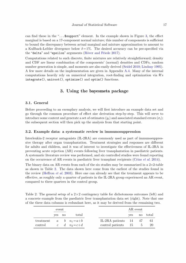
Interleukin-2 receptor antagonists (IL-2RA) are commonly used as part of immunosuppres-sive therapy after organ transplantation. Treatment strategies and responses are differentfor adults and children, and it was of interest to investigate the effectiveness of IL-2RA inpreventing acute rejection (AR) events following liver transplantation in paediatric patients.A systematic literature review was performed, and six controlled studies were found reportingon the occurrence of AR events in paediatric liver transplant recipients (Crins et al. 2014).
The binary data on AR events from each of the six studies may be summarized in a 2×2-tableas shown in Table 2. The data shown here come from the earliest of the studies found inthe review (Heffron et al. 2003). Here one can already see that the treatment appears to beeffective, as roughly only a quarter of patients in the IL-2RA group experienced an AR event,compared to three quarters in the control group.
Table 2: The general setup of a 2×2 contingency table for dichotomous outcomes (left) anda concrete example from the paediatric liver transplantation data set (right). Note that oneof the three data columns is redundant here, as it may be derived from the remaining two.
event
yes no total
treatment a b n1=a+bcontrol c d n2=c+d
AR event
yes no total
IL-2RA patients 14 47 61control patients 15 5 20
18 Meta-analysis using the bayesmeta package
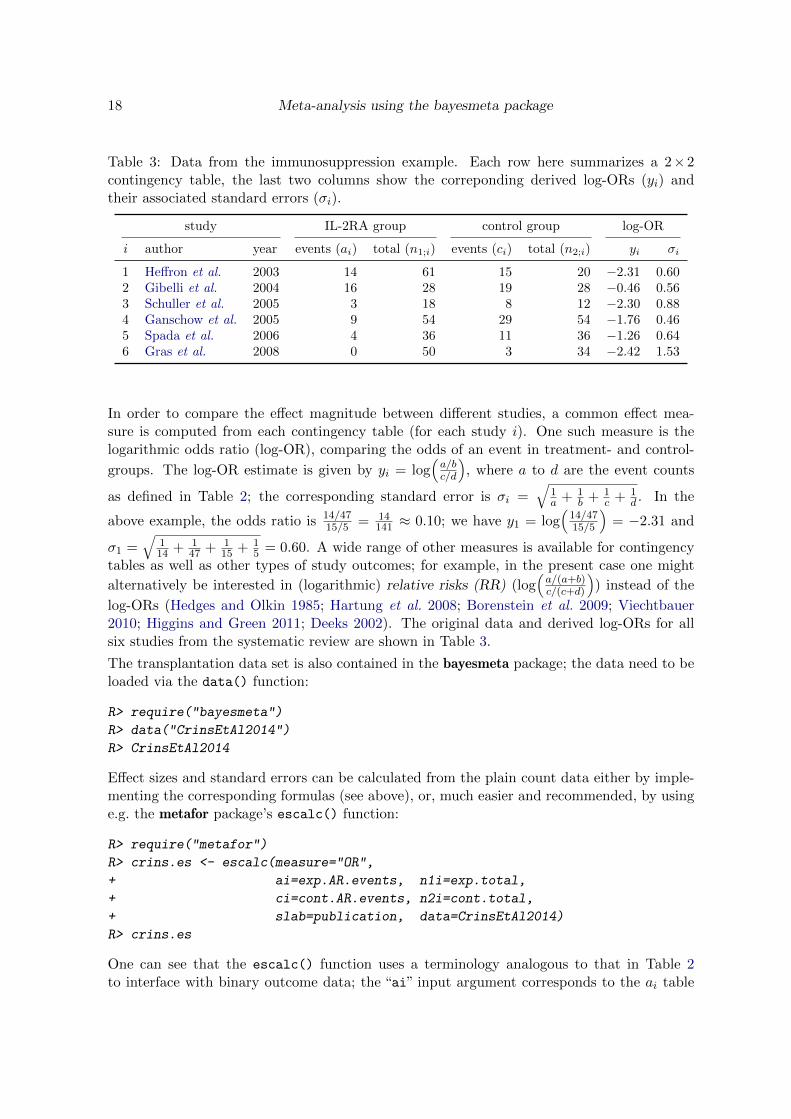
Table 3: Data from the immunosuppression example. Each row here summarizes a 2×2contingency table, the last two columns show the correponding derived log-ORs (yi) andtheir associated standard errors (σi).
study IL-2RA group control group log-OR
i author year events (ai) total (n1;i) events (ci) total (n2;i) yi σi
1 Heffron et al. 2003 14 61 15 20 −2.31 0.602 Gibelli et al. 2004 16 28 19 28 −0.46 0.563 Schuller et al. 2005 3 18 8 12 −2.30 0.884 Ganschow et al. 2005 9 54 29 54 −1.76 0.465 Spada et al. 2006 4 36 11 36 −1.26 0.646 Gras et al. 2008 0 50 3 34 −2.42 1.53
In order to compare the effect magnitude between different studies, a common effect mea-sure is computed from each contingency table (for each study i). One such measure is thelogarithmic odds ratio (log-OR), comparing the odds of an event in treatment- and control-
groups. The log-OR estimate is given by yi = log(a/bc/d
), where a to d are the event counts
as defined in Table 2; the corresponding standard error is σi =√
1a + 1
b + 1c + 1
d . In the
above example, the odds ratio is 14/4715/5 = 14
141 ≈ 0.10; we have y1 = log(14/4715/5
)= −2.31 and
σ1 =√
114 + 1
47 + 115 + 1
5 = 0.60. A wide range of other measures is available for contingencytables as well as other types of study outcomes; for example, in the present case one might
alternatively be interested in (logarithmic) relative risks (RR) (log(a/(a+b)c/(c+d)
)) instead of the
log-ORs (Hedges and Olkin 1985; Hartung et al. 2008; Borenstein et al. 2009; Viechtbauer2010; Higgins and Green 2011; Deeks 2002). The original data and derived log-ORs for allsix studies from the systematic review are shown in Table 3.
The transplantation data set is also contained in the bayesmeta package; the data need to beloaded via the data() function:
R> require("bayesmeta")
R> data("CrinsEtAl2014")
R> CrinsEtAl2014
Effect sizes and standard errors can be calculated from the plain count data either by imple-menting the corresponding formulas (see above), or, much easier and recommended, by usinge.g. the metafor package’s escalc() function:
R> require("metafor")
R> crins.es <- escalc(measure="OR",
+ ai=exp.AR.events, n1i=exp.total,
+ ci=cont.AR.events, n2i=cont.total,
+ slab=publication, data=CrinsEtAl2014)
R> crins.es
One can see that the escalc() function uses a terminology analogous to that in Table 2to interface with binary outcome data; the “ai” input argument corresponds to the ai table
Journal of Statistical Software 19
entries (number a of events in the treatment group for each study i), and so on. The outputof the escalc() function (here: the data frame named “crins.es”) will then be the originaldata along with two additional columns named “yi” and “vi” containing the calculated effectsizes (yi) and the squared (!) standard errors (σ2i ), respectively.
Note that for computing the 6th study’s log-OR (see Table 3), a continuity correction wasnecessary, because one of the contingency table entries was zero (Sweeting et al. 2004). Formore details on effect size calculation and default behaviour, see also Viechtbauer (2010) orthe escalc() function’s online documentation.
3.3. Performing a Bayesian random-effects meta-analysis
The bayesmeta() function
In order to perform a random-effects meta-analysis, we need to specify the data, as well asthe prior for the unknown parameters µ and τ (see Section 2.2). For the effect µ we arerestricted to normal or uniform priors; here we use a vague prior centered at µp = 0, whichcorresponds to a log-OR of 1, i.e., no effect. The prior standard deviation we set to σp = 4,corresponding to the vague unit information prior (see Section 2.2.2). For the heterogeneity,we use a half-normal prior with scale 0.5, confining the a priori expected heterogeneity toτ ≤ 0.98 with 95% probability (i.e., allowing for “fairly extreme” values with only about 5%prior probability).
With the log-ORs computed as in the previous section, we can now execute the analysis usingthe following call
R> ma01 <- bayesmeta(y = crins.es[,"yi"],
+ sigma = sqrt(crins.es[,"vi"]),
+ labels = crins.es[,"publication"],
+ mu.prior.mean = 0, mu.prior.sd = 4,
+ tau.prior = function(t){dhalfnormal(t,scale=0.5)})
The first three arguments pass the data (vectors of estimates yi and standard errors σi) and(optionally) a vector of corresponding study labels to the bayesmeta() function. Note that themetafor package’s escalc() function returned variances (i.e., squared standard errors), whilethe bayesmeta() function’s “sigma” argument requires the standard errors (i.e., the squareroot of the variances); hence the additional square-root-transformation here. The followingarguments specify the prior mean and standard deviation of the (normal) prior for the effect µ.Finally, the last argument specifies the prior for the heterogeneity τ . While for the effect priorwe are restricted to using normal (or improper uniform) priors, the heterogeneity prior canbe of essentially any type. Specification of the heterogeneity prior works via specification ofits prior density function. While this type of argument specification is somewhat unusual, itis reasonably straightforward, as one can see above. The dhalfnormal() function here is thehalf-normal distribution’s density function; see also the corresponding online help (e.g. viaentering “?dhalfnormal” in R).
Retrieving and processing the “yi” and “vi” elements (as well as study labels, if available)from an escalc() result in general is not complicated, and the bayesmeta() function canalso do this automatically for any escalc() output, including the many types of effect sizes
20 Meta-analysis using the bayesmeta package
that are available (Viechtbauer 2010). Using simply the escalc() function’s output as aninput, the identical result can be achieved by calling
R> ma01 <- bayesmeta(crins.es,
+ mu.prior.mean = 0, mu.prior.sd = 4,
+ tau.prior = function(t){dhalfnormal(t,scale=0.5)})
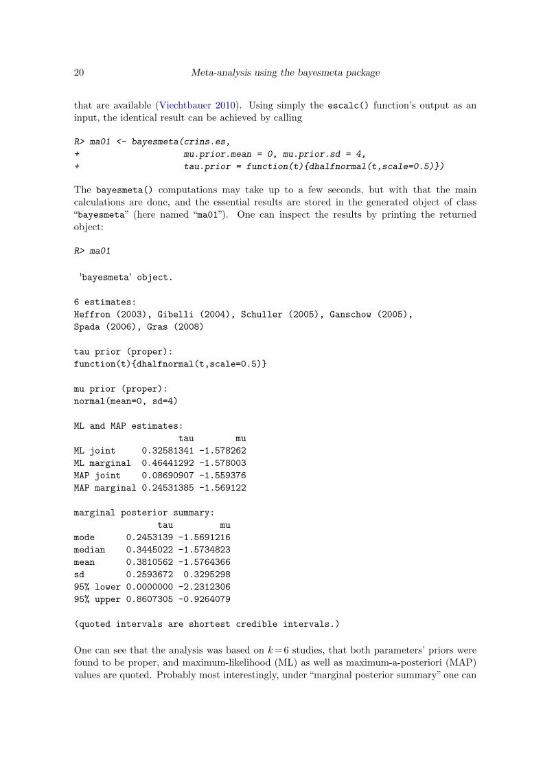
The bayesmeta() computations may take up to a few seconds, but with that the maincalculations are done, and the essential results are stored in the generated object of class“bayesmeta” (here named “ma01”). One can inspect the results by printing the returnedobject:
R> ma01
'bayesmeta' object.
6 estimates:
Heffron (2003), Gibelli (2004), Schuller (2005), Ganschow (2005),
Spada (2006), Gras (2008)
tau prior (proper):
function(t){dhalfnormal(t,scale=0.5)}
mu prior (proper):
normal(mean=0, sd=4)
ML and MAP estimates:
tau mu
ML joint 0.32581341 -1.578262
ML marginal 0.46441292 -1.578003
MAP joint 0.08690907 -1.559376
MAP marginal 0.24531385 -1.569122
marginal posterior summary:
tau mu
mode 0.2453139 -1.5691216
median 0.3445022 -1.5734823
mean 0.3810562 -1.5764366
sd 0.2593672 0.3295298
95% lower 0.0000000 -2.2312306
95% upper 0.8607305 -0.9264079
(quoted intervals are shortest credible intervals.)
One can see that the analysis was based on k= 6 studies, that both parameters’ priors werefound to be proper, and maximum-likelihood (ML) as well as maximum-a-posteriori (MAP)values are quoted. Probably most interestingly, under “marginal posterior summary” one can
Journal of Statistical Software 21
quoted estimate shrinkage estimate
study
Heffron (2003)
Gibelli (2004)
Schuller (2005)
Ganschow (2005)
Spada (2006)
Gras (2008)
mean
prediction
estimate
−2.31
−0.46
−2.30
−1.76
−1.26
−2.42
−1.57
−1.57
95% CI
[−3.48, −1.13]
[−1.55, 0.63]
[−4.03, −0.58]
[−2.65, −0.86]
[−2.52, −0.00]
[−5.41, 0.58]
[−2.23, −0.93]
[−2.77, −0.41]−5 −4 −3 −2 −1 0 1
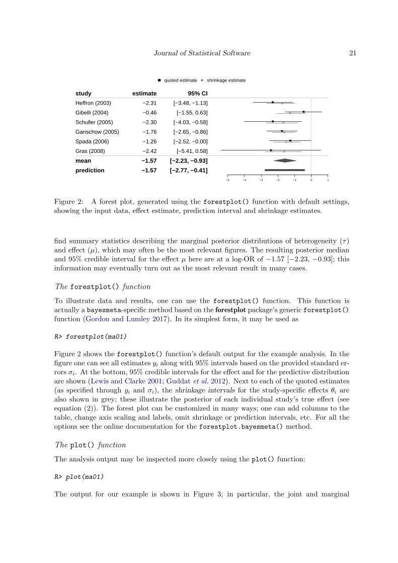
Figure 2: A forest plot, generated using the forestplot() function with default settings,showing the input data, effect estimate, prediction interval and shrinkage estimates.
find summary statistics describing the marginal posterior distributions of heterogeneity (τ)and effect (µ), which may often be the most relevant figures. The resulting posterior medianand 95% credible interval for the effect µ here are at a log-OR of −1.57 [−2.23, −0.93]; thisinformation may eventually turn out as the most relevant result in many cases.
The forestplot() function
To illustrate data and results, one can use the forestplot() function. This function isactually a bayesmeta-specific method based on the forestplot package’s generic forestplot()function (Gordon and Lumley 2017). In its simplest form, it may be used as
R> forestplot(ma01)
Figure 2 shows the forestplot() function’s default output for the example analysis. In thefigure one can see all estimates yi along with 95% intervals based on the provided standard er-rors σi. At the bottom, 95% credible intervals for the effect and for the predictive distributionare shown (Lewis and Clarke 2001; Guddat et al. 2012). Next to each of the quoted estimates(as specified through yi and σi), the shrinkage intervals for the study-specific effects θi arealso shown in grey; these illustrate the posterior of each individual study’s true effect (seeequation (2)). The forest plot can be customized in many ways; one can add columns to thetable, change axis scaling and labels, omit shrinkage or prediction intervals, etc. For all theoptions see the online documentation for the forestplot.bayesmeta() method.
The plot() function
The analysis output may be inspected more closely using the plot() function:
R> plot(ma01)
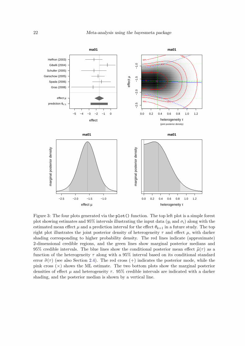
The output for our example is shown in Figure 3; in particular, the joint and marginal
22 Meta-analysis using the bayesmeta package
ma01
effect
Gras (2008)
Spada (2006)
Ganschow (2005)
Schuller (2005)
Gibelli (2004)
Heffron (2003)
prediction θk+1
effect µ
−5 −4 −3 −2 −1 0
ma01
(joint posterior density)
50%
90%
95% 99%
99%
99%
0.0 0.2 0.4 0.6 0.8 1.0 1.2
−2.
5−
2.0
−1.
5−
1.0
heterogeneity τ
effe
ct µ
effect µ
mar
gina
l pos
terio
r de
nsity
−2.5 −2.0 −1.5 −1.0
ma01
heterogeneity τ
mar
gina
l pos
terio
r de
nsity
0.0 0.2 0.4 0.6 0.8 1.0 1.2
ma01
Figure 3: The four plots generated via the plot() function. The top left plot is a simple forestplot showing estimates and 95% intervals illustrating the input data (yi and σi) along with theestimated mean effect µ and a prediction interval for the effect θk+1 in a future study. The topright plot illustrates the joint posterior density of heterogeneity τ and effect µ, with darkershading corresponding to higher probability density. The red lines indicate (approximate)2-dimensional credible regions, and the green lines show marginal posterior medians and95% credible intervals. The blue lines show the conditional posterior mean effect µ(τ) as afunction of the heterogeneity τ along with a 95% interval based on its conditional standarderror σ(τ) (see also Section 2.4). The red cross (+) indicates the posterior mode, while thepink cross (×) shows the ML estimate. The two bottom plots show the marginal posteriordensities of effect µ and heterogeneity τ . 95% credible intervals are indicated with a darkershading, and the posterior median is shown by a vertical line.
Journal of Statistical Software 23
posterior distributions are illustrated in detail. Prior densities may be superimposed by usingthe “prior=TRUE” argument, and axis ranges may also be specified manually; see also theonline help for the plot.bayesmeta() method.
Elements of the bayesmeta() output
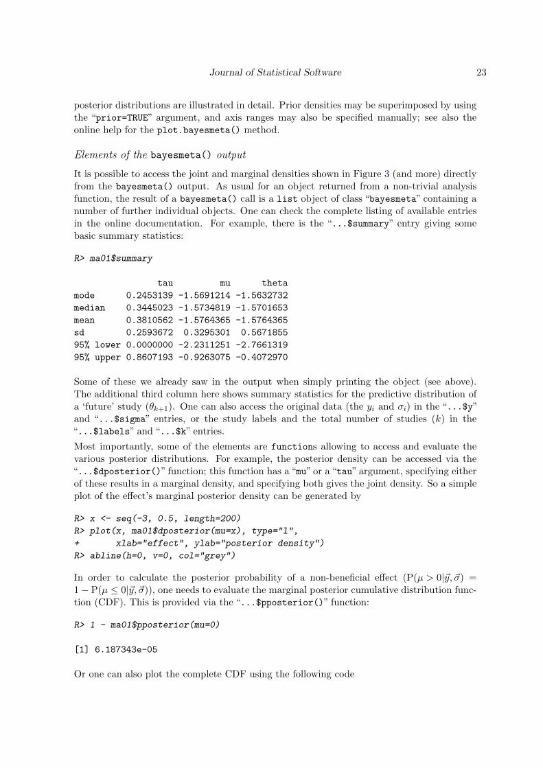
It is possible to access the joint and marginal densities shown in Figure 3 (and more) directlyfrom the bayesmeta() output. As usual for an object returned from a non-trivial analysisfunction, the result of a bayesmeta() call is a list object of class “bayesmeta” containing anumber of further individual objects. One can check the complete listing of available entriesin the online documentation. For example, there is the “...$summary” entry giving somebasic summary statistics:
R> ma01$summary
tau mu theta
mode 0.2453139 -1.5691214 -1.5632732
median 0.3445023 -1.5734819 -1.5701653
mean 0.3810562 -1.5764365 -1.5764365
sd 0.2593672 0.3295301 0.5671855
95% lower 0.0000000 -2.2311251 -2.7661319
95% upper 0.8607193 -0.9263075 -0.4072970
Some of these we already saw in the output when simply printing the object (see above).The additional third column here shows summary statistics for the predictive distribution ofa ‘future’ study (θk+1). One can also access the original data (the yi and σi) in the “...$y”and “...$sigma” entries, or the study labels and the total number of studies (k) in the“...$labels” and “...$k” entries.
Most importantly, some of the elements are functions allowing to access and evaluate thevarious posterior distributions. For example, the posterior density can be accessed via the“...$dposterior()” function; this function has a “mu” or a “tau” argument, specifying eitherof these results in a marginal density, and specifying both gives the joint density. So a simpleplot of the effect’s marginal posterior density can be generated by
R> x <- seq(-3, 0.5, length=200)
R> plot(x, ma01$dposterior(mu=x), type="l",
+ xlab="effect", ylab="posterior density")
R> abline(h=0, v=0, col="grey")
In order to calculate the posterior probability of a non-beneficial effect (P(µ > 0|~y, ~σ) =1− P(µ ≤ 0|~y, ~σ)), one needs to evaluate the marginal posterior cumulative distribution func-tion (CDF). This is provided via the “...$pposterior()” function:
R> 1 - ma01$pposterior(mu=0)
[1] 6.187343e-05
Or one can also plot the complete CDF using the following code

24 Meta-analysis using the bayesmeta package
R> x <- seq(-3, 0.5, length=200)
R> plot(x, ma01$pposterior(mu=x), type="l",
+ xlab="effect", ylab="posterior CDF")
R> abline(h=0:1, v=0, col="grey")
The same works also for the heterogeneity parameter τ ; in order to derive for example theposterior probability for a “fairly extreme” heterogeneity (τ > 1), one simply needs to supplythe “tau” parameter instead:
R> 1 - ma01$pposterior(tau=1)
[1] 0.02097488
so the posterior probability is at 2.1% here. The quantile function (inverse CDF) is alsoavailable in the “...$qposterior()” function; in order to derive for example a 99% upperlimit on the heterogeneity parameter, one needs to evaluate
R> ma01$qposterior(tau.p=0.99)
[1] 1.109186
so the 99% upper limit would here be at τ = 1.11.
In many cases it is useful to use Monte Carlo simulation to derive other non-trival quantitiesfrom the posterior distribution. One can generate samples from the posterior distributionusing the “...$rposterior()” function. A call of
R> ma01$rposterior(n=5)
tau mu
[1,] 0.23423926 -1.380271
[2,] 0.28630556 -1.442691
[3,] 0.04402682 -1.610052
[4,] 0.83672662 -1.550758
[5,] 0.18981184 -1.803012
will generate a sample of 5 draws from the joint (bivariate) posterior distribution of τ and µ.If one is only interested in the marginal distribution of µ, it is (substantially!) more efficientto omit the τ draws and use
R> ma01$rposterior(n=5, tau.sample=FALSE)
[1] -2.184596 -1.876711 -1.514224 -1.384694 -1.567397
to generate a vector of µ values only.
For example, suppose that we assume a rate of AR events of pc = 50% for the control group,and we are interested in the implied risk difference based on our analysis. The risk differenceis simply pt − pc, where pt is the event rate in the treatment (IL-2RA) group. To determinethe distribution of the risk difference we can now simply use Monte Carlo sampling and run
Journal of Statistical Software 25
R> prob.control <- 0.5
R> logodds.control <- log(prob.control / (1 - prob.control))
R> logodds.treat <- (logodds.control
+ + ma01$rposterior(n=10000, tau.sample=FALSE))
R> prob.treat <- exp(logodds.treat) / (1 + exp(logodds.treat))
R> riskdiff <- (prob.treat - prob.control)
R> median(riskdiff)
[1] -0.3284975
R> quantile(riskdiff, c(0.025, 0.975))
2.5% 97.5%
-0.4028368 -0.2149175
So here we find a median risk difference of −0.33 and a 95% credible interval of [−0.40, −0.21]for this example. The risk difference distribution could now also be investigated further usinghistograms etc.
Credible intervals
Central credible intervals can be computed using the corresponding posterior quantiles viathe “...$qposterior()” function (see above). By default however, shortest intervals (seeSection 2.9) are provided in the bayesmeta() output, or they can also be computed usingthe ...$post.interval() function. The bayesmeta() function’s default behaviour maybe controlled by setting the “interval.type” argument. Looking at Figure 3 (marginalposteriors at the bottom), one can see that, depending on the posterior’s shape, the shortestintervals may turn out one- or two-sided, at least for the heterogeneity parameter. For examplea 99% credible interval for the heterogeneity can then be computed via
R> ma01$post.interval(tau.level=0.99)
[1] 0.000000 1.109186
attr(,"interval.type")
[1] "shortest"
One can also see that the returned interval contains an attribute indicating the type of in-terval. A central interval then is derived by explicitly specifying the method to be used forcomputation:
R> ma01$post.interval(tau.level=0.99, method="central")
[1] 0.003547657 1.205400562
attr(,"interval.type")
[1] "central"
Such an interval then is actually simply based on the corresponding “central” quantiles, asone can check by running:
26 Meta-analysis using the bayesmeta package
−3 −2 −1 0
0.0
0.5
1.0
1.5
effect
prob
abili
ty d
ensi
typosterior (µ)posterior predictive (θk+1)
−4 −3 −2 −1 0
0.0
0.2
0.4
0.6
0.8
1.0
1.2
effect
prob
abili
ty d
ensi
ty
initial estimate (y1 ± σ1)shrinkage estimate (θ1|y,σ)
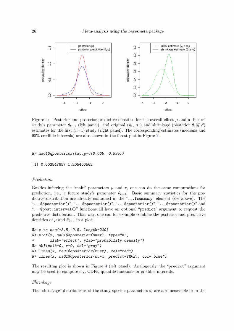
Figure 4: Posterior and posterior predictive densities for the overall effect µ and a ‘future’study’s parameter θk+1 (left panel), and original (y1, σ1) and shrinkage (posterior θ1|~y, ~σ)estimates for the first (i=1) study (right panel). The corresponding estimates (medians and95% credible intervals) are also shown in the forest plot in Figure 2.
R> ma01$qposterior(tau.p=c(0.005, 0.995))
[1] 0.003547657 1.205400562
Prediction
Besides inferring the “main” parameters µ and τ , one can do the same computations forprediction, i.e., a future study’s parameter θk+1. Basic summary statistics for the pre-dictive distribution are already contained in the “...$summary” element (see above). The“...$dposterior()”, “...$pposterior()”, “...$qposterior()”, “...$rposterior()” and“...$post.interval()” functions all have an optional “predict” argument to request thepredictive distribution. That way, one can for example combine the posterior and predictivedensities of µ and θk+1 in a plot:
R> x <- seq(-3.5, 0.5, length=200)
R> plot(x, ma01$dposterior(mu=x), type="n",
+ xlab="effect", ylab="probability density")
R> abline(h=0, v=0, col="grey")
R> lines(x, ma01$dposterior(mu=x), col="red")
R> lines(x, ma01$dposterior(mu=x, predict=TRUE), col="blue")
The resulting plot is shown in Figure 4 (left panel). Analogously, the “predict” argumentmay be used to compute e.g. CDFs, quantile functions or credible intervals.
Shrinkage
The “shrinkage” distributions of the study-specific parameters θi are also accessible from the
Journal of Statistical Software 27
bayesmeta() output. They are also summarized in the “...$theta” element; for example,shrinkage for the first two studies is shown in the first two columns:
R> ma01$theta[,1:2]
Heffron (2003) Gibelli (2004)
y -2.3097026 -0.4595323
sigma 0.5994763 0.5563956
mode -1.6711220 -1.3895876
median -1.7411356 -1.2821722
mean -1.7778965 -1.2339736
sd 0.4229425 0.4488759
95% lower -2.6561049 -2.0455088
95% upper -0.9920023 -0.3089461
One can see the original data (yi and σi) along with the posterior summaries (see also the for-est plot in Figure 2). The “...$dposterior()”, “...$pposterior()”, “...$qposterior()”,“...$rposterior()”and“...$post.interval()”functions again also have an optional“individual”argument to specify one of the individual studies (either by their index or by their name).For example, one can illustrate the first study’s (i = 1) input data (y1, σ1) and shrinkageestimate (θ1) in a single plot using the following code
R> x <- seq(-4, 0.5, length=200)
R> plot(x, ma01$dposterior(theta=x, individual=1), type="n",
+ xlab="effect", ylab="probability density")
R> abline(h=0, v=0, col="grey")
R> lines(x, dnorm(x, mean=ma01$y[1], sd=ma01$sigma[1]),
+ col="green", lty="dashed")
R> lines(x, ma01$dposterior(theta=x, individual=1), col="green")
The resulting two densities are shown in Figure 4 (right panel). Analogously, the“individual”argument may be used to compute e.g. CDFs, quantile functions or credible intervals.
3.4. Investigating prior variations
Prior predictive distributions
In order to judge the implications of settings of the heterogeneity prior, it is often useful toconsider prior predictive distributions (Gelman et al. 2014). Any fixed value of τ will implya certain (prior) distribution and variability among the true study-specific means θ1, . . . , θk,namely, a normal distribution with Var(θi|τ) = τ2. Depending on the type of endpoint (e.g.,log-ORs), the implied variability can be interpreted and judged on the corresponding outcomescale (Spiegelhalter et al. 2004, Sec. 5.7).
Assuming a prior distribution for τ , rather than a fixed value, also implies assumptions onthe a priori expected distribution and variability of the true study parameters θi. The priorpredictive distribution of the θi values then is a mixture of normal distributions, with mean µand with the prior p(τ) as the mixing distribution for the normal standard deviation (Seidel
28 Meta-analysis using the bayesmeta package
2010; Lindsay 1995). As the name suggests, the prior predictive distribution is actually closelyrelated to the (posterior) predictive distribution discussed above (Gelman et al. 2014). Thismixture distribution can again be evaluated using the direct algorithm (Rover and Friede2017); this approach is implemented in the normalmixture() function.
Consider the half-normal prior distribution with scale 0.5 that was used for the heterogene-ity in the above analysis. We can now check what prior predictive distribution this priorcorresponds to. We only need to supply the prior CDF (the mean µ is by default set to zero):
R> hn05 <- normalmixture(cdf=function(t){phalfnormal(t, scale=0.5)})
One can check the returned result (e.g. via str(hn05)); the result is a list with severalelements, among which most importantly are the mixture’s density, cumulative distributionand quantile functions (“...$density()”, “...$cdf()” and “...$quantile()”, respectively).
For comparison, we can also check the implications of a half-Cauchy prior of the same scale,or a half-normal prior of doubled scale:
R> hn10 <- normalmixture(cdf=function(t){phalfnormal(t, scale=1.0)})
R> hc05 <- normalmixture(cdf=function(t){phalfcauchy(t, scale=0.5)})
and compare these graphically via their implied prior predictive CDFs by accessing the threemixtures’ “...$cdf()” functions:
R> x <- seq(-1, 3, by=0.01)
R> plot(x, hn05$cdf(x), type="l", col="blue", ylim=0:1,
+ xlab=expression(theta[i]), ylab="prior predictive CDF")
R> lines(x, hn10$cdf(x), col="green")
R> lines(x, hc05$cdf(x), col="red")
R> abline(h=0:1, v=0, col="grey")
R> axis(3, at=log(c(0.5,1,2,5,10,20)), lab=c(0.5,1,2,5,10,20))
R> mtext(expression(exp(theta[i])), side=3, line=2.5)
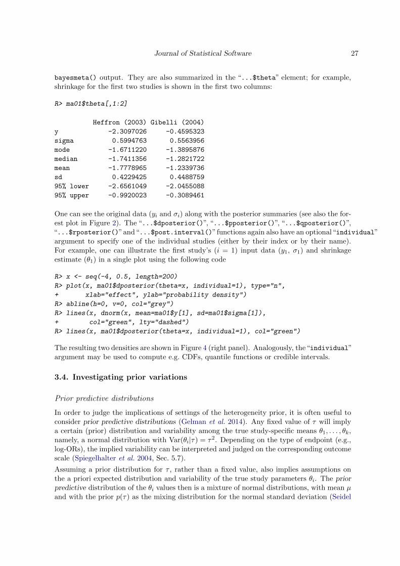
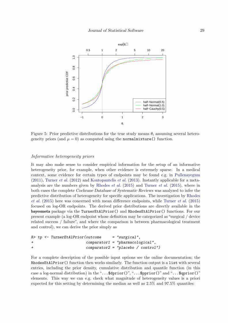
The resulting plot is shown in Figure 5. In our example, the effect measure is a log-OR, sothe θi need to be interpreted on the exponentiated scale (see the top axis). A priori, 95% ofθi values are assumed to be within ± the 97.5% quantile of the (symmetric) prior predictivedistribution. We can now check what this means for our three cases:
R> q975 <- c("half-normal(0.5)" = hn05$quantile(0.975),
+ "half-normal(1.0)" = hn10$quantile(0.975),
+ "half-Cauchy(0.5)" = hc05$quantile(0.975))
R> print(cbind("theta"=q975, "exp(theta)"=exp(q975)))
theta exp(theta)
half-normal(0.5) 1.092287 2.981083
half-normal(1.0) 2.184573 8.886857
half-Cauchy(0.5) 5.050571 156.111517
So for the half-normal prior with scale 0.5 we have 95% probability roughly within a factorof 1
3 or 3 around the overall mean odds ratio (exp(µ)). For the other two priors, the numbersare much more extreme.
Journal of Statistical Software 29
−1 0 1 2 3
0.0
0.2
0.4
0.6
0.8
1.0
θi
prio
r pr
edic
tive
CD
F
half−Normal(0.5)half−Normal(1.0)half−Cauchy(0.5)
0.5 1 2 5 10 20
exp(θi)
Figure 5: Prior predictive distributions for the true study means θi assuming several hetero-geneity priors (and µ = 0) as computed using the normalmixture() function.
Informative heterogeneity priors
It may also make sense to consider empirical information for the setup of an informativeheterogeneity prior, for example, when other evidence is extremely sparse. In a medicalcontext, some evidence for certain types of endpoints may be found e.g. in Pullenayegum(2011), Turner et al. (2012) and Kontopantelis et al. (2013). Instantly applicable for a meta-analysis are the numbers given by Rhodes et al. (2015) and Turner et al. (2015), where inboth cases the complete Cochrane Database of Systematic Reviews was analyzed to infer thepredictive distribution of heterogeneity for specific applications. The investigation by Rhodeset al. (2015) here was concerned with mean difference endpoints, while Turner et al. (2015)focused on log-OR endpoints. The derived prior distributions are directly available in thebayesmeta package via the TurnerEtAlPrior() and RhodesEtAlPrior() functions. For ourpresent example (a log-OR endpoint whose definition may be categorized as “surgical / devicerelated success / failure”, and where the comparison is between pharmacological treatmentand control), we can derive the prior simply as
R> tp <- TurnerEtAlPrior(outcome = "surgical",
+ comparator1 = "pharmacological",
+ comparator2 = "placebo / control")
For a complete description of the possible input options see the online documentation; theRhodesEtAlPrior() function then works similarly. The function output is a list with severalentries, including the prior density, cumulative distribution and quantile function (in thiscase a log-normal distribution) in the “...$dprior()”, “...$pprior()” and “...$qprior()”elements. This way we can e.g. check what magnitude of heterogeneity values is a prioriexpected for this setting by determining the median as well as 2.5% and 97.5% quantiles:
30 Meta-analysis using the bayesmeta package
R> tp$qprior(c(0.025, 0.5, 0.975))
[1] 0.06233896 0.34300852 1.88734045
The prior density can now immediately be used and passed on to the bayesmeta() function;for example, we can use the same effect prior as before and the “empirical” prior for theheterogeneity:
R> ma02 <- bayesmeta(crins.es,
+ mu.prior.mean = 0, mu.prior.sd = 4,
+ tau.prior = tp$dprior)
Comparing the results to the previous analysis (e.g. via their “...$summary” outputs), onecan see that in this case they are very similar. The two corresponding prior densities are alsoshown in Figure 1 (page 11; solid and dotted blue lines).
Non-informative priors
As discussed in Section 2.2, an obvious choice of an uninformative prior for the effect µwould be the (improper) uniform prior on the real line; this one can be utilized by simplyleaving the mu.prior.mean and mu.prior.sd parameters unspecified. In order to use oneof the uninformative heterogeneity priors discussed in Section 2.2, these do not need to bespecified “manually” in terms of their probability density function; a set of priors is alreadypre-implemented and may be specified via a character string. The default setting for exampleis tau.prior="uniform". If one wants to use, say, the uniform effect prior along with theJeffreys prior for the heterogeneity τ (see Section 2.2 and Bodnar et al. (2017)), one can run
R> ma03 <- bayesmeta(crins.es, tau.prior="Jeffreys")
The complete list of possible options is described in detail in the online documentation.
3.5. Making the connection with frequentist results
Frequentist and Bayesian approaches to inference within the NNHM framework are obviouslyrelated, and it may be interesting to highlight the connection between the correspondingresults. A simple frequentist analysis may be performed e.g. using the metafor package’s“rma()” function via
R> ma04 <- rma(crins.es)
(Viechtbauer 2010). By default, the restricted ML (REML) heterogeneity estimator τREML isused, but the type of estimator does not matter here. The heterogeneity point estimate hereturns out as:
R> sqrt(ma04$tau2)
[1] 0.4670268
and we can retrieve the effect estimate and its standard error via:
Journal of Statistical Software 31
R> ma04$b
[,1]
intrcpt -1.591513
R> ma04$se
[1] 0.3340882
In the Bayesian setup, these numbers correspond to conditional posterior moments of theeffect (µ|τ = τREML) in an analysis using the uniform effect prior. Such an analysis wasperformed in the previous subsection (uniform effect prior and Jeffreys heterogeneity prior;the heterogeneity prior does not matter here) and stored in the “ma03” object. From thiswe can retrieve the effect’s conditional posterior moments (mean and standard deviation forτ= τREML) using the “...$cond.moment()” function:
R> ma03$cond.moment(tau = sqrt(ma04$tau2))
mean sd
[1,] -1.591513 0.3340882
and we can see that these correspond exactly to the frequentist effect estimate. Both analysisapproaches are related through the use of the same likelihood function; in the Bayesiananalysis uncertainty (e.g. in the heterogeneity) is accounted for via integration, and a priordistribution for both parameters is considered.
3.6. Posterior predictive checks
A meta-analysis of two studies
Posterior predictive p-values allow to quantify the consistency of the data with certain para-metric hypotheses; see Section 2.10. In the following we will determine some p-values fromthe bayesmeta() output; to this end, we will investigate a second meta-analysis exampleinvolving only two studies.
Of the six studies considered in the pediatric transplantation example (see Figure 2), onlytwo were randomized (Heffron et al. 2003; Spada et al. 2006). Since randomized studies areusually considered as evidence of higher quality, now suppose one was interested in combiningthe randomized studies only. Computations analogous to the preceding example may be donevia
R> ma05 <- bayesmeta(crins.es[crins.es[,"randomized"]=="yes",],
+ mu.prior.mean=0, mu.prior.sd=4,
+ tau.prior=function(t){dhalfnormal(t,scale=0.5)})
Figure 6 shows the forest plot for this analysis. Based on these two studies only, we can nowinspect e.g. the estimate of the overall effect µ; comparing to the previous analysis (Figure 2),the (absolute) estimate is slightly larger, but the credible interval is wider.
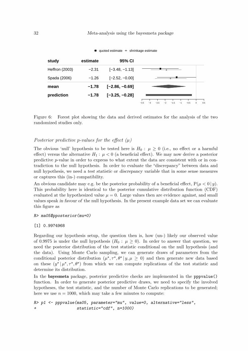
32 Meta-analysis using the bayesmeta package
quoted estimate shrinkage estimate
study
Heffron (2003)
Spada (2006)
mean
prediction
estimate
−2.31
−1.26
−1.78
−1.78
95% CI
[−3.48, −1.13]
[−2.52, −0.00]
[−2.86, −0.69]
[−3.25, −0.28]
−3.5 −3 −2.5 −2 −1.5 −1 −0.5 0 0.5
Figure 6: Forest plot showing the data and derived estimates for the analysis of the tworandomized studies only.
Posterior predictive p-values for the effect (µ)
The obvious ‘null’ hypothesis to be tested here is H0 : µ ≥ 0 (i.e., no effect or a harmfuleffect) versus the alternative H1 : µ < 0 (a beneficial effect). We may now derive a posteriorpredictive p-value in order to express to what extent the data are consistent with or in con-tradiction to the null hypothesis. In order to evaluate the “discrepancy” between data andnull hypothesis, we need a test statistic or discrepancy variable that in some sense measuresor captures this (in-) compatibility.
An obvious candidate may e.g. be the posterior probability of a beneficial effect, P(µ < 0 | y).This probability here is identical to the posterior cumulative distribution function (CDF)evaluated at the hypothesized value µ = 0. Large values then are evidence against, and smallvalues speak in favour of the null hypothesis. In the present example data set we can evaluatethis figure as
R> ma05$pposterior(mu=0)
[1] 0.9974968
Regarding our hypothesis setup, the question then is, how (un-) likely our observed valueof 0.9975 is under the null hypothesis (H0 : µ ≥ 0). In order to answer that question, weneed the posterior distribution of the test statistic conditional on the null hypothesis (andthe data). Using Monte Carlo sampling, we can generate draws of parameters from theconditional posterior distribution (µ?, τ?, θ? | y, µ ≥ 0) and then generate new data basedon these (y? |µ?, τ?, θ?) from which we can compute replications of the test statistic anddetermine its distribution.
In the bayesmeta package, posterior predictive checks are implemented in the pppvalue()
function. In order to generate posterior predictive draws, we need to specify the involvedhypotheses, the test statistic, and the number of Monte Carlo replications to be generated;here we use n = 1000, which may take a few minutes to compute:
R> p1 <- pppvalue(ma05, parameter="mu", value=0, alternative="less",
+ statistic="cdf", n=1000)
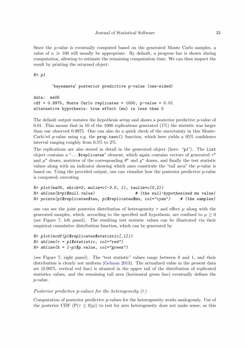
Journal of Statistical Software 33
Since the p-value is eventually computed based on the generated Monte Carlo samples, avalue of n � 100 will usually be appropriate. By default, a progress bar is shown duringcomputation, allowing to estimate the remaining computation time. We can then inspect theresult by printing the returned object:
R> p1
'bayesmeta' posterior predictive p-value (one-sided)
data: ma05
cdf = 0.9975, Monte Carlo replicates = 1000, p-value = 0.01
alternative hypothesis: true effect (mu) is less than 0
The default output restates the hypothesis setup and shows a posterior predictive p-value of0.01. This means that in 10 of the 1000 replications generated (1%) the statistic was largerthan our observed 0.9975. One can also do a quick check of the uncertainty in this Monte-Carlo’ed p-value using e.g. the prop.test() function, which here yields a 95% confidenceinterval ranging roughly from 0.5% to 2%.
The replications are also stored in detail in the generated object (here: “p1”). The list
object contains a “...$replicates” element, which again contains vectors of generated τ?
and µ? draws, matrices of the corresponding θ? and y? draws, and finally the test statisticvalues along with an indicator showing which ones constitute the “tail area” the p-value isbased on. Using the provided output, one can visualize how the posterior predictive p-valueis computed; executing
R> plot(ma05, which=2, mulim=c(-3.5, 1), taulim=c(0,2))
R> abline(h=p1$null.value) # (the null-hypothesized mu value)
R> points(p1$replicates$tau, p1$replicates$mu, col="cyan") # (the samples)
one can see the joint posterior distribution of heterogeneity τ and effect µ along with thegenerated samples, which, according to the specified null hypothesis, are confined to µ ≥ 0(see Figure 7, left panel). The resulting test statistic values can be illustrated via theirempirical cumulative distribution function, which can be generated by
R> plot(ecdf(p1$replicates$statistic[,1]))
R> abline(v = p1$statistic, col="red")
R> abline(h = 1-p1$p.value, col="green")
(see Figure 7, right panel). The “test statistic” values range between 0 and 1, and theirdistribution is clearly not uniform (Gelman 2013). The actualized value in the present dataset (0.9975, vertical red line) is situated in the upper tail of the distribution of replicatedstatistics values, and the remaining tail area (horizontal green line) eventually defines thep-value.
Posterior predictive p-values for the heterogeneity (τ)
Computation of posterior predictive p-values for the heterogeneity works analogously. Use ofthe posterior CDF (P(τ ≤ 0|y)) to test for zero heterogeneity does not make sense, as this
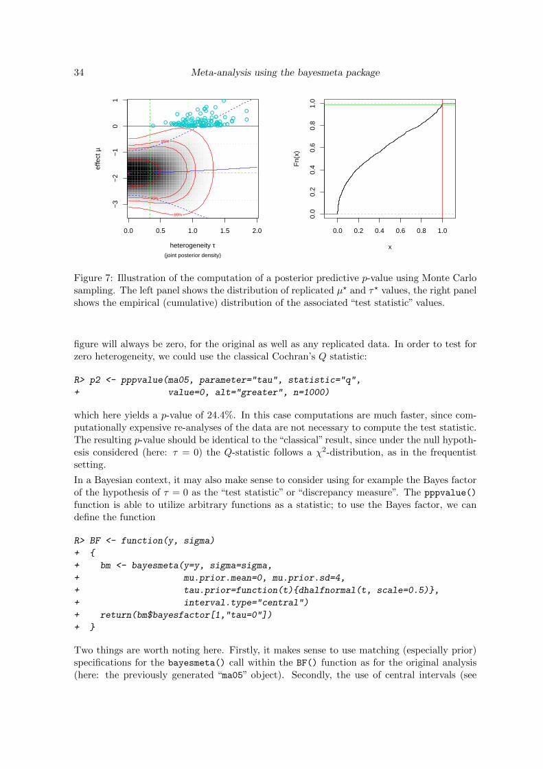
34 Meta-analysis using the bayesmeta package
(joint posterior density)
50%
90%
95%
99%
0.0 0.5 1.0 1.5 2.0
−3
−2
−1
01
heterogeneity τ
effe
ct µ
●
●●
●●
●
●
●●●
●● ●●● ●
●
●●
●
●
●●
●●
●
●●
●
●
●●
●●
●
●●
●●
●●● ●● ●●
●
●●
●●●
●●
●
●● ●
●
●● ●●●●
● ●●
●● ●●
● ●
●
●●●●●●
●
●
●●
●
● ●●● ●
●
●
●
●
● ●●
●●
0.0 0.2 0.4 0.6 0.8 1.0
0.0
0.2
0.4
0.6
0.8
1.0
x
Fn(
x)
Figure 7: Illustration of the computation of a posterior predictive p-value using Monte Carlosampling. The left panel shows the distribution of replicated µ? and τ? values, the right panelshows the empirical (cumulative) distribution of the associated “test statistic” values.
figure will always be zero, for the original as well as any replicated data. In order to test forzero heterogeneity, we could use the classical Cochran’s Q statistic:
R> p2 <- pppvalue(ma05, parameter="tau", statistic="q",
+ value=0, alt="greater", n=1000)
which here yields a p-value of 24.4%. In this case computations are much faster, since com-putationally expensive re-analyses of the data are not necessary to compute the test statistic.The resulting p-value should be identical to the “classical” result, since under the null hypoth-esis considered (here: τ = 0) the Q-statistic follows a χ2-distribution, as in the frequentistsetting.
In a Bayesian context, it may also make sense to consider using for example the Bayes factorof the hypothesis of τ = 0 as the “test statistic” or “discrepancy measure”. The pppvalue()
function is able to utilize arbitrary functions as a statistic; to use the Bayes factor, we candefine the function
R> BF <- function(y, sigma)
+ {
+ bm <- bayesmeta(y=y, sigma=sigma,
+ mu.prior.mean=0, mu.prior.sd=4,
+ tau.prior=function(t){dhalfnormal(t, scale=0.5)},
+ interval.type="central")
+ return(bm$bayesfactor[1,"tau=0"])
+ }
Two things are worth noting here. Firstly, it makes sense to use matching (especially prior)specifications for the bayesmeta() call within the BF() function as for the original analysis(here: the previously generated “ma05” object). Secondly, the use of central intervals (see
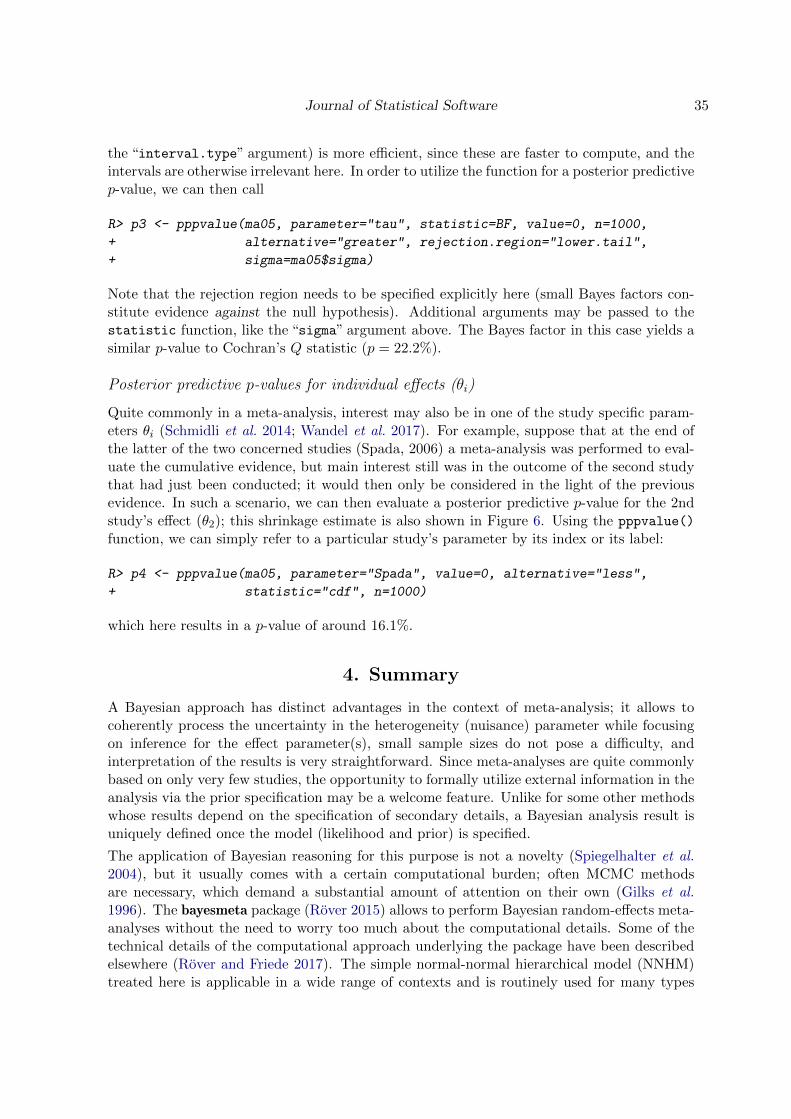
Journal of Statistical Software 35
the “interval.type” argument) is more efficient, since these are faster to compute, and theintervals are otherwise irrelevant here. In order to utilize the function for a posterior predictivep-value, we can then call
R> p3 <- pppvalue(ma05, parameter="tau", statistic=BF, value=0, n=1000,
+ alternative="greater", rejection.region="lower.tail",
+ sigma=ma05$sigma)
Note that the rejection region needs to be specified explicitly here (small Bayes factors con-stitute evidence against the null hypothesis). Additional arguments may be passed to thestatistic function, like the “sigma” argument above. The Bayes factor in this case yields asimilar p-value to Cochran’s Q statistic (p = 22.2%).
Posterior predictive p-values for individual effects (θi)
Quite commonly in a meta-analysis, interest may also be in one of the study specific param-eters θi (Schmidli et al. 2014; Wandel et al. 2017). For example, suppose that at the end ofthe latter of the two concerned studies (Spada, 2006) a meta-analysis was performed to eval-uate the cumulative evidence, but main interest still was in the outcome of the second studythat had just been conducted; it would then only be considered in the light of the previousevidence. In such a scenario, we can then evaluate a posterior predictive p-value for the 2ndstudy’s effect (θ2); this shrinkage estimate is also shown in Figure 6. Using the pppvalue()
function, we can simply refer to a particular study’s parameter by its index or its label:
R> p4 <- pppvalue(ma05, parameter="Spada", value=0, alternative="less",
+ statistic="cdf", n=1000)
which here results in a p-value of around 16.1%.
4. Summary
A Bayesian approach has distinct advantages in the context of meta-analysis; it allows tocoherently process the uncertainty in the heterogeneity (nuisance) parameter while focusingon inference for the effect parameter(s), small sample sizes do not pose a difficulty, andinterpretation of the results is very straightforward. Since meta-analyses are quite commonlybased on only very few studies, the opportunity to formally utilize external information in theanalysis via the prior specification may be a welcome feature. Unlike for some other methodswhose results depend on the specification of secondary details, a Bayesian analysis result isuniquely defined once the model (likelihood and prior) is specified.
The application of Bayesian reasoning for this purpose is not a novelty (Spiegelhalter et al.2004), but it usually comes with a certain computational burden; often MCMC methodsare necessary, which demand a substantial amount of attention on their own (Gilks et al.1996). The bayesmeta package (Rover 2015) allows to perform Bayesian random-effects meta-analyses without the need to worry too much about the computational details. Some of thetechnical details of the computational approach underlying the package have been describedelsewhere (Rover and Friede 2017). The simple normal-normal hierarchical model (NNHM)treated here is applicable in a wide range of contexts and is routinely used for many types
36 Meta-analysis using the bayesmeta package
of input data and effect measures (Hedges and Olkin 1985; Hartung et al. 2008; Viechtbauer2010; Borenstein et al. 2009). The bayesmeta implementation allows for quick, accurate andreproducible computation, and it has already faciltated some larger-scale simulation studiesto compare Bayesian results with common alternative approaches and evaluate their relativeperformance (Friede et al. 2017a,b). Usage of the bayesmeta package is not more compli-cated to use than many other common meta-analysis tools. The availability of predictivedistributions and shrinkage estimates makes the package attractive also for advanced evi-dence synthesis applications, like extrapolation to future studies (Schmidli et al. 2014, 2017;Wandel et al. 2017). Since the generic NNHM appears in different fields of application, useof the bayesmeta package may also be extended to other areas of research beyond commonmeta analysis. For example, it could as well be used to model hierarchical structures withina study (e.g., groups of patients), or a two-stage approach may be useful for meta-analysisbased on individual-patient data. In future, the same numerical approach might be extendedto the more general case of meta-regression.
A. Appendix
A.1. Unit information priors for binary outcomes
Logarithmic odds ratios (log-OR)
If the effect measure of an analysis is a logarithmic odds ratio (log-OR; see Section 3.2),
then the standard error derived from a 2×2 contingency table amounts to√
1a + 1
b + 1c + 1
d ,
where a, b, c and d are the four entries (counts) and N = a+ b+ c+ d is the total number ofsubjects (Hedges and Olkin 1985; Hartung et al. 2008; Borenstein et al. 2009). Assuming equalallocation and a neutral effect, we can simply set the table allocation to a = b = c = d = N
4 . Ifwe further plug in a total sample size of N = 1, this leads (heuristically) to a unit informationprior for the log-OR with zero mean and a standard deviation of 4. For this prior distribution,logarithmic odds are within a range of ±7.84 with 95% probability, corresponding to oddsroughly within a range from 1
2500 to 2500.
If more generally we consider the case of a particular event probability p ∈ [0, 1], we canderive a unit information prior by assuming a = c = pN2 and b = d = (1−p)N2 , leading to agenerally even larger prior standard deviation of 2√
p(1−p).
Logarithmic relative risks (log-RR)
Similarly to the previous section, the logarithmic relative risk (log-RR) is given by log(a/(a+b)c/(c+d)
),
and its associated standard error is√
1a −
1a+b + 1
c −1c+d (Hedges and Olkin 1985; Hartung
et al. 2008; Borenstein et al. 2009). Again plugging in a = b = c = d = N4 , this now amounts
to a standard deviation of 2. If we introduce a certain event probability p (and plugging in
a = c = pN2 and a+ b = c+ d = N2 , the error is 2
√1−pp , which is larger for p < 1
2 and smaller
for p > 12 .

Journal of Statistical Software 37
A.2. Conservatism of the uniform heterogeity prior
As discussed in Section 2.2, it is hard to define an “uninformative” prior for the heterogeneityparameter τ . A larger heterogeneity will first of all generally lead to a larger variance ofthe effect’s marginal posterior (via the larger variance of the conditional distribution; seeequations (17), (21)). One may then argue that an overestimation of heterogeneity may beconsidered a conservative form of bias, so that, for example, among two exponential priordistributions the one with the larger expectation was “more conservative” in a certain sense.
A shift in heterogeneity causes a change in both the conditional standard deviation and mean.If the shift in µ(τ) happens to be larger than the shift in σ(τ), then the resulting (conditional)confidence interval for a larger heterogeneity value does not necessarily completely contain theinterval corresponding to a smaller heterogeneity. Such cases may then lead to counterintuitiveresults for (frequentist) fixed- and random-effects analysis results especially in settings withimbalanced standard errors (Poole and Greenland 1999). Although it is not obvious whethersuch pathologies are also realistic in a Bayesian analysis, a priori, this is unlikely to lead toany systematic bias.
Nevertheless, along these lines it is possible to show a particular “conservatism” property forthe improper uniform prior. The derivation goes as follows. Suppose we have a boundedparameter domain [a,∞], a likelihood function f(x) ≥ 0 (x ∈ [a,∞]) with
∫∞a f(x) dx < ∞,
and a prior with monotonically decreasing probability density function p(·), so that 0 < p(a) <∞, and a ≤ x < y ⇒ 0 ≤ p(y) ≤ p(x). Using the (improper) uniform prior or prior p we getdifferent posteriors with cumulative distribution functions F1(·) and Fp(·), respectively. Fromthe above assumptions follows that
Fp(y) =
∫ ya f(x) p(x) dx∫∞a f(x) p(x) dx
≥∫ ya f(x) p(y) dx∫∞a f(x) p(a) dx
=p(y)
p(a)
∫ ya f(x) dx∫∞a f(x) dx
(30)
≥∫ ya f(x) dx∫∞a f(x) dx
= F1(y) (31)
for all y > a. This means that with Fp(y) ≥ F1(y), the posterior using the uniform prior isstochastically larger than the posterior based on any other prior among the class of priorswith monotonically decreasing density p(·) and finite p(a) (provided the uniform prior yields aproper posterior). In our context, this especially implies that quantiles or expectations basedon the uniform prior are larger (Shaked and Shanthikumar 2007).
The class of priors with finite intercept and monotonically decreasing density to which theabove property applies includes e.g. the exponential, half-normal, half-Student-t, half-Cauchyand Lomax distributions (Johnson et al. 1994), or uniform distributions with a finite upperbound.
A.3. Marginal likelihood derivation
Using the improper uniform prior for µ (p(µ) ∝ 1), the marginal likelihood, marginalizedover µ, is
p(~y|τ, ~σ) =
∫p(~y|µ, τ, ~σ) p(µ) dµ (32)
= (2π)−k2 ×
k∏i=1
1√σ2i +τ2
×∫
exp
(−1
2
k∑i=1
(yi − µ)2
σ2i +τ2
)dµ (33)
38 Meta-analysis using the bayesmeta package
where
k∑i=1
(yi − µ)2
σ2i + τ2=
k∑i=1
y2iσ2i + τ2︸ ︷︷ ︸=:a
+µ
(−2
k∑i=1
yiσ2i + τ2
)︸ ︷︷ ︸
=:b
+µ2k∑i=1
1
σ2i + τ2︸ ︷︷ ︸=:c
(34)
= a+ b µ+ c µ2 (35)
=(µ− −b2c )2√
1/c2 + a− b2
4c =(µ− µ(τ))2
σ(τ)2+ ∆(τ) (36)
and
µ(τ) =−b2c
=
∑ki=1
yiσ2i +τ
2∑ki=1
1σ2i +τ
2
(37)
σ(τ) =√
1/c =
√√√√ 1∑ki=1
1σ2i +τ
2
(38)
∆(τ) = a− b2
4c =k∑i=1
y2iσ2i + τ2
−
(∑ki=1
yiσ2i +τ
2
)2∑ki=1
1σ2i +τ
2
. (39)
=k∑i=1
1
σ2i + τ2
(yi −
k∑j=1
1σ2j+τ
2 yj∑k`=1
1σ2`+τ2
)2
=k∑i=1
(yi − µ(τ))2
σ2i + τ2. (40)
Note that µ(τ) (37) and σ(τ) (38) are the conditional posterior mean and standard deviationof µ|τ . With that the marginal likelihood turns out as
p(~y|τ, ~σ) = (2π)−k2 ×
k∏i=1
1√σ2i + τ2
×∫
exp
(−1
2
(µ− µ(τ))2
σ2(τ)− 1
2∆(τ)
)dµ (41)
= (2π)−k2 ×
k∏i=1
1√σ2i + τ2
× exp(−12∆(τ))×
∫exp
(−1
2
(µ− µ(τ))2
σ2(τ)
)dµ(42)
= (2π)−k2 ×
k∏i=1
1√σ2i + τ2
× exp(−12∆(τ))×
√2π σ(τ) (43)
= (2π)−k−12 ×
k∏i=1
1√σ2i + τ2
× exp
(−1
2
(yi − µ(τ))2
σ2i + τ2
)× 1√∑k
i=11
σ2i +τ
2
. (44)
The derivation for an informative normal effect prior (with mean µp and variance σ2p) workssimilarly.
A.4. Mixture implementation details
The approximation of marginal effect distributions etc. is implemented via the direct algo-rithm as described by Rover and Friede (2017). This approximation is utilized to evaluate
Journal of Statistical Software 39
posterior distributions of the overall effect µ as well as shrinkage estimates θi and predic-tions θk+1. In all three cases, the distributions of interest are mixtures of conditionallynormal distributions; in order to construct the approximate discrete mixture, it is necessaryto evaluate symmetrized divergences of the conditional distributions. The symmetrized di-vergence (relative entropy) for two normal distributions with mean and variance parameters(µA, σ
2A) and (µB, σ
2B), respectively, is given by
Ds(p(ϑ|µA, σA)‖p(ϑ|µB, σB)) = (µA−µB)2
( 12(σ−2
A +σ−2B ))
−1 +(σ2
A−σ2B)2
2σ2A σ
2B
(45)
(Rover and Friede 2017). Since the conditional means of µ|τ and θk+1|τ are identical, whilethe conditional variance of the latter is always equal to or larger than the former (see Sec-tion 2.8), a grid constructed for the effect’s posterior (µ) can always be used for the predictivedistribution (θk+1) without loss of accuracy. In order not to have to construct and considerseveral separate τ grids also for the different shrinkage distributions, the general algorithm isslightly extended. Instead of determining divergences corresponding to pairs of τ values withrespect to each of the shrinkage distributions individually, the maximum divergence acrosseffect posterior as well as all k shrinkage distributions is considered. The result is a singlegrid in τ values that may be re-used for all three types of distributions.
Acknowledgements
This project has received funding from the European Union’s Seventh Framework Programmefor research, technological development and demonstration under grant agreement numberFP HEALTH 2013-602144 through the InSPiRe project. Much of the present work evolved inclose collaboration with Tim Friede, Beat Neuenschwander and Simon Wandel. Many thanksfor helpful comments and proofreading go to Thomas Asendorf, Burak Gunhan, MarkusHarden, Judith Heinz, Barbora Kessel, Tobias Mutze, Sibylle Sturtz and Steffen Unkel.
References
Bender R, Kuß O, Koch A, Schwenke C, Hauschke D (2014). “Application of predictionintervals in meta-analyses with random effects.” Joint Statement of IQWiG, GMDSand IBS-DR. URL: https://www.iqwig.de/download/2014-03-07_Joint_Statement_
Prediction_Intervals.pdf.
Berger J, Pericchi LR (2001). “Objective Bayesian methods for model selection: Introductionand comparison.” In P Lahiri (ed.), Model Selection, volume 38 of IMS Lecture Notes,pp. 135–193. Institute of Mathematical Statistics, Beachwood, OH. doi:10.1214/lnms/
1215540968.
Berger JO (1985). Statistical decision theory and Bayesian analysis. 2nd edition. Springer-Verlag.
Berger JO, Deely J (1988). “A Bayesian approach to ranking and selection of related meanswith alternatives to analysis-of-variance methodology.” Journal of the American StatisticalAssociation, 83(402), 364–373. doi:10.1080/01621459.1988.10478606.
40 Meta-analysis using the bayesmeta package
Berkhof J, van Mechelen I, Hoijting H (2000). “Posterior predictive checks: Principles anddiscussion.” Computational Statistics, 15(3), 337–354. doi:10.1007/s001800000038.
Bodnar O, Link A, Arendacka B, Possolo A, Elster C (2017). “Bayesian estimation in randomeffects meta-analysis using a non-informative prior.” Statistics in Medicine, 36(2), 378–399.doi:10.1002/sim.7156.
Bodnar O, Link A, Elster C (2016). “Objective Bayesian inference for a generalized marginalrandom effects model.” Bayesian Analysis, 11(1), 25–45. doi:10.1214/14-BA933.
Borenstein M, Hedges LV, Higgins JPT, Rothstein HR (2009). Introduction to Meta-Analysis.Wiley & Sons.
Chalmers I, Hedges LV, Cooper H (2002). “A brief history of research synthesis.” Evaluation& the Health Professions, 25(1), 12–37. doi:10.1177/0163278702025001003.
Chambert T, Rotella JJ, Higgs MD (2014). “Use of posterior predictive checks as an inferentialtool for investigating individual heterogeneity in animal population vital rates.” Ecologyand Evolution, 4(8), 1389–1397. doi:10.1002/ece3.993.
Chung Y, Rabe-Hesketh S, Choi IH (2013). “Avoiding zero between-study variance estimatesin random-effects meta-analysis.” Statistics in Medicine, 32(23), 4071–4089. doi:10.1002/sim.5821.
Crins ND, Rover C, Goralczyk AD, Friede T (2014). “Interleukin-2 receptor antagonists forpediatric liver transplant recipients: A systematic review and meta-analysis of controlledstudies.” Pediatric Transplantation, 18(8), 839–850. doi:10.1111/petr.12362.
Daniels M (1999). “A prior for the variance in hierarchical models.” The Candian Journal ofStatistics, 27(3), 567–578. doi:10.2307/3316112.
Davey J, Turner RM, Clarke MJ, Higgins JPT (2011). “Characteristics of meta-analysesand their component studies in the Cochrane Database of Systematic Reviews: a cross-sectional, descriptive analysis.” BMC Medical Research Methodology, 11(1), 160. doi:
10.1186/1471-2288-11-160.
Deeks JJ (2002). “Issues in the selection of a summary statistic for meta-analysis of clinicaltrials with binary outcomes.” Statistics in Medicine, 21(11), 1575–1600. doi:10.1002/
sim.1188.
DuMouchel WH, Normand SL (2000). “Computer modeling strategies for meta-analysis.” InDK Stangl, DA Berry (eds.), Meta-analysis in medicine and health policy, pp. 127–178.CRC Press.
Follmann DA, Proschan MA (1999). “Valid inference in random effects meta-analysis.” Bio-metrics, 55(3), 732–737. doi:10.1111/j.0006-341X.1999.00732.x.
Friede T, Rover C, Wandel S, Neuenschwander B (2017a). “Meta-analysis of few small studiesin orphan diseases.” Research Synthesis Methods, 8(1), 79–91. doi:10.1002/jrsm.1217.
Friede T, Rover C, Wandel S, Neuenschwander B (2017b). “Meta-analysis of two studiesin the presence of heterogeneity with applications in rare diseases.” Biometrical Journal,59(4), 658–671. doi:10.1002/bimj.201500236.
Journal of Statistical Software 41
Friedrich T, Knapp G (2013). “Generalized interval estimation in the random effects metaregression model.” Computational Statistics & Data Analysis, 64, 165–179. doi:10.1016/j.csda.2013.03.011.
Ganschow R, Grabhorn E, Schulz A, von Hugo A, Rogiers X, Burdelski A (2005). “Long-termresults of basiliximab induction immunosuppression in pediatric liver transplant recipients.”Pediatric Transplantation, 9(6), 741–745. doi:10.1111/j.1399-3046.2005.00371.x.
Gelman A (2003). “A Bayesian formulation of exploratory data analysis and goodness-of-fittesting.” International Statistical Review, 71(2), 369–382. doi:10.1111/j.1751-5823.
2003.tb00203.x.
Gelman A (2006). “Prior distributions for variance parameters in hierarchical models.”Bayesian Analysis, 1(3), 515–534. doi:10.1214/06-BA117A.
Gelman A (2013). “Two simple examples for understanding posterior p-values whose dis-tributions are far from uniform.” Electronic Journal of Statistics, 7, 2595–2602. doi:
10.1214/13-EJS854.
Gelman A, Carlin JB, Stern H, Dunson DB, Vehtari A, Rubin DB (2014). Bayesian dataanalysis. 3rd edition. Chapman & Hall / CRC, Boca Raton.
Gelman A, Meng XL, Stern H (1996). “Posterior predictive assessment of model fitness viarealized discrepancies.” Statistica Sinica, 6(4), 733–760. URL http://www.jstor.org/
stable/24306036.
Gibelli NEM, Pinho-Apezzato ML, Miyatani HT, Maksoud-Filho JG, Silva MM, Ayoub AAR,Santos MM, Velhote MCP, Tannuri U, Maksoud JG (2004). “Basiliximab-chimeric anti-IL2-R monoclonal antibody in pediatric liver transplantation: comparative study.” Trans-plantation Proceedings, 36(4), 956–957. doi:10.1016/j.transproceed.2004.04.070.
Gilks WR, Richardson S, Spiegelhalter DJ (1996). Markov chain Monte Carlo in practice.Chapman & Hall / CRC, Boca Raton.
Gordon M, Lumley T (2017). “forestplot: Advanced forest plot using ‘grid’ graphics.” R pack-age version 1.7.2, URL http://cran.r-project.org/package=forestplot.
Gras JM, Gerkens S, Beguin C, Janssen M, Smets F, Otte JB, Sokal E, Reding R (2008).“Steroid-free, tacrolimus-basiliximab immunosuppression in pediatric liver transplantation:Clinical and pharmacoeconomic study in 50 children.” Liver Transplantation, 14(4), 469–477. doi:10.1002/lt.21397.
Gregory PC (2005). Bayesian logical data analysis for the physical sciences. CambridgeUniversity Press, Cambridge.
Guddat C, Grouven U, Bender R, Skipka G (2012). “A note on the graphical presentationof prediction intervals in random-effects meta-analyses.” Systematic Reviews, 1(34). doi:
10.1186/2046-4053-1-34.
Hartung J, Knapp G (2001a). “On tests of the overall treatment effect in meta-analysiswith normally distributed responses.” Statistics in Medicine, 20(12), 1771–1782. doi:
10.1002/sim.791.
42 Meta-analysis using the bayesmeta package
Hartung J, Knapp G (2001b). “A refined method for the meta-analysis of controlled clinicaltrials with binary outcome.” Statistics in Medicine, 20(24), 3875–3889. doi:10.1002/sim.1009.
Hartung J, Knapp G, Sinha BK (2008). Statistical meta-analysis with applications. Wiley,Hoboken, NJ, USA.
Hedges LV, Olkin I (1985). Statistical methods for meta-analysis. Academic Press, San Diego,CA, USA.
Heffron TG, Pillen T, Smallwood GA, Welch D, Oakley B, Romero R (2003). “Pediatric livertransplantation with daclizumab induction therapy.” Transplantation, 75(12), 2040–2043.doi:10.1097/01.TP.0000065740.69296.DA.
Higgins JPT, Green S (eds.) (2011). Cochrane handbook for systematic reviews of interven-tions. Version 5.1.0, URL http://handbook.cochrane.org/.
Higgins JPT, Thompson SG (2002). “Quantifying heterogeneity in a meta-analysis.” Statisticsin Medicine, 21(11), 1539–1558. doi:10.1002/sim.1186.
Higgins JPT, Thompson SG, Spiegelhalter DJ (2009). “A re-evaluation of random-effectsmeta-analysis.” Journal of the Royal Statistical Society A, 172(1), 137–159. doi:10.1111/j.1467-985X.2008.00552.x.
Jaynes ET (1968). “Prior probabilities.” IEEE Transactions on Systems Science and Cyber-netics, SEC-4(3), 227–241. doi:10.1109/TSSC.1968.300117.
Jaynes ET (1976). “Confidence intervals vs. Bayesian intervals.” In WL Harper, CA Hooker(eds.), Foundations of probability theory, statistical inference, and statistical theories ofscience, pp. 175–257. D. Reidel, Dordrecht. doi:10.1007/978-94-010-1436-6_6.
Jaynes ET (2003). Probability theory: The logic of science. Cambridge University Press,Cambridge.
Jeffreys H (1946). “An invariant form for the prior probability in estimation problems.”Proceedings of the Royal Society of London, Series A, 186(1007), 453–461. doi:10.1098/
rspa.1946.0056.
Jeffreys H (1961). Theory of probability. 3rd edition. Clarendon Press, Oxford.
Johnson NL, Kotz S, Balakrishnan N (1994). Continuous univariate distributions. 2nd edition.Wiley, New York.
Kacker RN, Forbes A, Kessel R, Sommer KD (2008). “Bayesian posterior predictive p-valueof statistical consistency in interlaboratory evaluations.” Metrologia, 45(5), 512–523. doi:10.1088/0026-1394/45/5/004.
Kass RE, Wasserman L (1995). “A reference Bayesian test for nested hypotheses and itsrelationship to the Schwarz criterion.” Journal of the American Statistical Association,90(431), 928–934. doi:10.2307/2291327.
Journal of Statistical Software 43
Kass RE, Wasserman L (1996). “The selection of prior distributions by formal rules.” Jour-nal of the American Statistical Association, 91(435), 1343–1370. doi:10.1080/01621459.1996.10477003.
Kontopantelis E, Springate DA, Reeves D (2013). “A re-analysis of the Cochrane Library data:The dangers of unobserved heterogeneity in meta-analyses.” PLoS ONE, 8(7), e69930. doi:10.1371/journal.pone.0069930.
Lewis S, Clarke M (2001). “Forest plots: trying to see the wood and the trees.” BMJ,322(7300), 1479–1480. doi:10.1136/bmj.322.7300.1479.
Liberati A, Altman DG, Tetzlaff J, Mulrow C, Gøtzsche PC, Ioannidis JPA, Clarke M, Dev-ereaux PJ, Kleijnen J, Moher D (2009). “The PRISMA statement for reporting systematicreviews and meta-analyses of studies that evaluate health care interventions: explanationand elaboration.” PLoS Medicine, 6(7), e1000100. doi:10.1371/journal.pmed.1000100.
Lindley DV (1977). “The distinction between inference and decision.” Synthese, 36(1), 51–58.doi:10.1007/BF00485691.
Lindsay BG (1995). Mixture models: theory, geometry and applications, volume 5 of NSF-CBMS Regional Conference Series in Probability and Statistics. Institute of MathematicalStatistics, Hayward, CA, USA. URL http://www.jstor.org/stable/4153184.
Lunn D, Barrett J, Sweeting A, Thompson S (2013). “Fully Bayesian hierarchical modellingin two stages with application to meta-analysis.” Journal of the Royal Statistical Society C,62(4), 551–572. doi:10.1111/rssc.12007.
Mandelkern M (2002). “Setting confidence intervals for bounded parameters.” StatisticalScience, 17(2), 149–172. doi:10.1214/ss/1030550859.
Meng XL (1994). “Posterior predictive p-values.” The Annals of Statistics, 22(3), 1142–1160.doi:10.1214/aos/1176325622.
Metropolis N, Ulam S (1949). “The Monte Carlo method.” Journal of the American StatisticalAssociation, 44(247), 335–341. doi:10.1080/01621459.1949.10483310.
O’Hagan A, Pericchi L (2012). “Bayesian heavy-tailed models and conflict resolution: Areview.” Brazilian Journal of Probability and Statistics, 26(4), 372–401. doi:10.1214/
11-BJPS164.
Polson NG, Scott JG (2012). “On the half-Cauchy prior for a global scale parameter.”BayesianAnalysis, 7(4), 887–902. doi:10.1214/12-BA730.
Poole C, Greenland S (1999). “Random-effects meta-analyses are not always conservative.”American Journal of Epidemiology, 150(5), 469–475. doi:10.1093/oxfordjournals.aje.a010035.
Pullenayegum EM (2011). “An informed reference prior for between-study heterogeneityin meta-analyses of binary outcomes.” Statistics in Medicine, 30(26), 3082–3094. doi:
10.1002/sim.4326.
44 Meta-analysis using the bayesmeta package
Rhodes KM, Turner RM, Higgins JPT (2015). “Predictive distributions were developed for theextent of heterogeneity in meta-analyses of continuous outcome data.” Journal of ClinicalEpidemiology, 68(1), 52–60. doi:10.1016/j.jclinepi.2014.08.012.
Riley RD, Higgins JP, Deeks JJ (2011). “Interpretation of random effects meta-analyses.”BMJ, 342, d549. doi:10.1136/bmj.d549.
Rover C (2015). “bayesmeta: Bayesian random-effects meta analysis.” R package. URL:http://cran.r-project.org/package=bayesmeta.
Rover C, Friede T (2017). “Discrete approximation of a mixture distribution via restricteddivergence.” Journal of Computational and Graphical Statistics, 26(1), 217–222. doi:
10.1080/10618600.2016.1276840.
Rucker G, Schumacher M (2008). “Simpson’s paradox visualized: The example of Rosigli-tazone meta-analysis.” BMC Medical Research Methodology, 8, 34. doi:10.1186/
1471-2288-8-34.
Schmidli H, Gsteiger S, Roychoudhury S, O’Hagan A, Spiegelhalter D, Neuenschwander B(2014). “Robust meta-analytic-predictive priors in clinical trials with historical controlinformation.” Biometrics, 70(4), 1023–1032. doi:10.1111/biom.12242.
Schmidli H, Neuenschwander B, Friede T (2017). “Meta-analytic-predictive use of historicalvariance data for the design and analysis of clinical trials.” Computational Statistics & DataAnalysis, 113, 100–110. doi:10.1016/j.csda.2016.08.007.
Schuller S, Wiederkehr JC, Coelho-Lemos IM, Avilla SG, Schultz C (2005). “Daclizumabinduction therapy associated with tacrolimus-MMF has better outcome compared withtacrolimus-MMF alone in pediatric living donor liver transplantation.” TransplantationProceedings, 37(2), 1151–1152. doi:10.1016/j.transproceed.2005.01.023.
Schwarzer G (2007). “meta: An R package for meta-analysis.” R News, 7(3), 40–45.
Schwarzer G, Carpenter JR, Rucker G (2015). Meta-Analysis with R. Springer.
Seidel WE (2010). “Mixture models.” In M Lovric (ed.), International Encyclopedia of Sta-tistical Science, pp. 827–829. Springer, Heidelberg. doi:10.1007/978-3-642-04898-2.
Senn S (2007). “Trying to be precise about vagueness.” Statistics in Medicine, 26(7), 1417–1430. doi:10.1002/sim.2639.
Shaked M, Shanthikumar JG (2007). Stochastic orders. Springer, New York.
Sidik K, Jonkman JN (2002). “A simple confidence interval for meta-analysis.” Statistics inMedicine, 21(21), 3153–3159. doi:10.1002/sim.1262.
Sinharay S, Johnson MJ, Stern HS (2006). “Posterior predictive assessment of item re-sponse theory models.” Applied Psychological Measurement, 30(4), 298–321. doi:
10.1177/0146621605285517.
Smith TC, Spiegelhalter DJ, Thomas A (1995). “Bayesian approaches to random-effectsmeta-analysis: A comparative study.” Statistics in Medicine, 14(24), 2685–2699. doi:
10.1002/sim.4780142408.

Journal of Statistical Software 45
Spada M, Petz W, Bertani A, Riva S, Sonzogni A, Giovannelli M, Torri E, Torre G, ColledanM, Gridelli B (2006). “Randomized trial of basiliximab induction versus steroid therapy inpediatric liver allograft recipients under tacrolimus immunosuppression.” American Journalof Transplantation, 6(8), 1913–1921. doi:10.1111/j.1600-6143.2006.01406.x.
Spiegelhalter DJ (2004). “Incorporating Bayesian ideas into health-care evaluation.”StatisticalScience, 19(1), 156–174. doi:10.1214/088342304000000080.
Spiegelhalter DJ, Abrams KR, Myles JP (2004). Bayesian approaches to clinical trials andhealth-care evaluation. Wiley & Sons.
Spiegelhalter DJ, Myles JP, Jones DR, Abrams KR (1999). “An introduction to Bayesianmethods in health technology assessment.” BMJ, 319, 508–512. doi:10.1136/bmj.319.
7208.508.
Sutton AJ, Abrams KR (2001). “Bayesian methods in meta-analysis and evidence syn-thesis.” Statistical Methods in Medical Research, 10(4), 277–303. doi:10.1177/
096228020101000404.
Sweeting MJ, Sutton AJ, Lambert PC (2004). “What to add to nothing? Use and avoidanceof continuity corrections in meta-analysis of sparse data.” Statistics in Medicine, 23(9),1351–1375. doi:10.1002/sim.1761.
Tibshirani R (1989). “Noninformative priors for one parameter of many.” Biometrika, 76(3),604–608. doi:10.1093/biomet/76.3.604.
Turner RM, Davey J, Clarke MJ, Thompson SG, Higgins JPT (2012). “Predicting the extentof heterogeneity in meta-analysis, using empirical data from the Cochrane Database ofSystematic Reviews.” International Journal of Epidemiology, 41(3), 818–827. doi:10.
1093/ije/dys041.
Turner RM, Jackson D, Wei Y, Thompson SG, Higgins PT (2015). “Predictive distributionsfor between-study heterogeneity and simple methods for their application in Bayesian meta-analysis.” Statistics in Medicine, 34(6), 984–998. doi:10.1002/sim.6381.
van de Schoot R, Kaplan D, Denissen J, Asendorpf JB, Neyer FJ, van Aken MAG (2014). “Agentle introduction to Bayesian analysis: Applications to developmental research.” ChildDevelopment, 85(3), 842–860. doi:10.1111/cdev.12169.
Veroniki AA, Jackson D, Viechtbauer W, Bender R, Bowden J, Knapp G, Kuß O, HigginsJPT, Langan D, Salanti G (2016). “Methods to estimate the between-study variance andits uncertainty in meta-analysis.” Research Synthesis Methods, 7(1), 55–79. doi:10.1002/jrsm.1164.
Viechtbauer W (2010). “Conducting meta-analyses in R with the metafor package.” Journalof Statistical Software, 36(3). doi:10.18637/jss.v036.i03.
Wandel S, Neuenschwander B, Friede T, Rover C (2017). “Using phase II data for the analysisof phase III studies: an application in rare diseases.” Clinical Trials, 14(3), 277–285. doi:10.1177/1740774517699409.
46 Meta-analysis using the bayesmeta package
Wasserstein RL (2016). “ASA statement on statistical significance and p-values.” The Amer-ican Statistician, 70(2), 131–133. doi:10.1080/00031305.2016.1154108.
Affiliation:
Christian RoverDepartment of Medical StatisticsUniversity Medical Center GottingenGeorg-August-Universitat37073 Gottingen, GermanyE-mail: [email protected]: http://www.gwdg.de/~croeverORCID iD: 0000-0002-6911-698X
Journal of Statistical Software http://www.jstatsoft.org/
published by the Foundation for Open Access Statistics http://www.foastat.org/
MMMMMM YYYY, Volume VV, Issue II Submitted: 2017-11-23doi:10.18637/jss.v000.i00 Accepted: yyyy-mm-dd