Bayesian Optimization with Unknown Constraints

Michael A. Gelbart, Jasper Snoek, and Ryan P. Adams

School of Engineering and Applied Sciences, Harvard University

{mgelbart, jsnoek, rpa} @ seas.harvard.edu

Abstract

Recent work on Bayesian optimization has shown its effectiveness in global optimization ofdifficult black-box objective functions. Many real-world optimization problems of interest alsohave constraints which are unknown a priori. In this paper, we study Bayesian optimization forconstrained problems in the general case that noise may be present in the constraint functions,and the objective and constraints may be evaluated independently. We provide motivating prac-tical examples, and present a general framework to solve such problems. We demonstrate theeffectiveness of our approach on optimizing the performance of online latent Dirichlet allocationsubject to topic sparsity constraints, tuning a neural network given test-time memory constraints,and optimizing Hamiltonian Monte Carlo to achieve maximal effectiveness in a fixed time, subjectto passing standard convergence diagnostics.

1 Introduction

Bayesian optimization (Mockus et al., 1978) is a method for performing global optimization of un-known “black box” objectives that is particularly appropriate when objective function evaluations areexpensive (in any sense, such as time or money). For example, consider a food company trying todesign a low-calorie variant of a popular cookie. In this case, the design space is the space of possiblerecipes and might include several key parameters such as quantities of various ingredients and bakingtimes. Each evaluation of a recipe entails computing (or perhaps actually measuring) the number ofcalories in the proposed cookie. Bayesian optimization can be used to propose new candidate recipessuch that good results are found with few evaluations.

Now suppose the company also wants to ensure the taste of the cookie is not compromised whencalories are reduced. Therefore, for each proposed low-calorie recipe, they perform a taste test withsample customers. Because different people, or the same people at different times, have differingopinions about the taste of cookies, the company decides to require that at least 95% of test subjectsmust like the new cookie. This is a constrained optimization problem:

minx

c(x) s.t. ρ(x) ≥ 1− ε ,

where x is a real-valued vector representing a recipe, c(x) is the number of calories in recipe x, ρ(x)is the fraction of test subjects that like recipe x, and 1− ε is the minimum acceptable fraction, i.e.,95%.

This paper presents a general formulation of constrained Bayesian optimization that is suitable fora large class of problems such as this one. Other examples might include tuning speech recognitionperformance on a smart phone such that the user’s speech is transcribed within some acceptable timelimit, or minimizing the cost of materials for a new bridge, subject to the constraint that all safetymargins are met.

1

arX

iv:1

403.

5607

v1 [

stat

.ML

] 2

2 M

ar 2

014

Another use of constraints arises when the search space is known a priori but occupies a compli-cated volume that cannot be expressed as simple coordinate-wise bounds on the search variables. Forexample, in a chemical synthesis experiment, it may be known that certain combinations of reagentscause an explosion to occur. This constraint is not unknown in the sense of being a discovered propertyof the environment as in the examples above—we do not want to discover the constraint boundary bytrial and error explosions of our laboratory. Rather, we would like to specify this constraint using aboolean noise-free oracle function that declares input vectors as valid or invalid. Our formulation ofconstrained Bayesian optimization naturally encapsulates such constraints.

1.1 Bayesian Optimization

Bayesian optimization proceeds by iteratively developing a global statistical model of the unknownobjective function. Starting with a prior over functions and a likelihood, at each iteration a posteriordistribution is computed by conditioning on the previous evaluations of the objective function, treatingthem as observations in a Bayesian nonlinear regression. An acquisition function is used to map beliefsabout the objective function to a measure of how promising each location in input space is, if it wereto be evaluated next. The goal is then to find the input that maximizes the acquisition function, andsubmit it for function evaluation.

Maximizing the acquisition function is ideally a relatively easy proxy optimization problem: eval-uations of the acquisition function are often inexpensive, do not require the objective to be queried,and may have gradient information available. Under the assumption that evaluating the objectivefunction is expensive, the time spent computing the best next evaluation via this inner optimizationproblem is well spent. Once a new result is obtained, the model is updated, the acquisition functionis recomputed, and a new input is chosen for evaluation. This completes one iteration of the Bayesianoptimization loop.

For an in-depth discussion of Bayesian optimization, see Brochu et al. (2010b) or Lizotte (2008).Recent work has extended Bayesian optimization to multiple tasks and objectives (Krause and Ong,2011; Swersky et al., 2013; Zuluaga et al., 2013) and high dimensional problems (Wang et al., 2013;Djolonga et al., 2013). Strong theoretical results have also been developed (Srinivas et al., 2010; Bull,2011; de Freitas et al., 2012). Bayesian optimization has been shown to be a powerful method forthe meta-optimization of machine learning algorithms (Snoek et al., 2012; Bergstra et al., 2011) andalgorithm configuration (Hutter et al., 2011).

1.2 Expected Improvement

An acquisition function for Bayesian optimization should address the exploitation vs. explorationtradeoff: the idea that we are interested both in regions where the model believes the objective functionis low (“exploitation”) and regions where uncertainty is high (“exploration”). One such choice is theExpected Improvement (EI) criterion (Mockus et al., 1978), an acquisition function shown to havestrong theoretical guarantees (Bull, 2011) and empirical effectiveness (e.g., Snoek et al., 2012). Theexpected improvement, EI(x), is defined as the expected amount of improvement over some target t,if we were to evaluate the objective function at x:

EI(x) = E[(t− y)+] =

∫ ∞−∞

(t− y)+p(y |x) dy , (1)

where p(y |x) is the predictive marginal density of the objective function at x, and (t− y)+ ≡ max(0, t− y)is the improvement (in the case of minimization) over the target t. EI encourages both exploitationand exploration because it is large for inputs with a low predictive mean (exploitation) and/or a highpredictive variance (exploration). Often, t is set to be the minimum over previous observations (e.g.,Snoek et al., 2012), or the minimum of the expected value of the objective (Brochu et al., 2010a).Following our formulation of the problem, we use the minimum expected value of the objective suchthat the probabilistic constraints are satisfied (see Section 1.5, Eq., 6).

2

When the predictive distribution under the model is Gaussian, EI has a closed-form expression(Jones, 2001):

EI(x) = σ(x) (z(x)Φ (z(x)) + φ (z(x))) (2)

where z(x) ≡ t−µ(x)σ(x) , µ(x) is the predictive mean at x, σ2(x) is the predictive variance at x, Φ(·) is the

standard normal CDF, and φ(·) is the standard normal PDF. This function is differentiable and fastto compute, and can therefore be maximized with a standard gradient-based optimizer. In Section 3we present an acquisition function for constrained Bayesian optimization based on EI.

1.3 Our Contributions

The main contribution of this paper is a general formulation for constrained Bayesian optimization,along with an acquisition function that enables efficient optimization of such problems. Our formu-lation is suitable for addressing a large class of constrained problems, including those considered inprevious work. The specific improvements are enumerated below.

First, our formulation allows the user to manage uncertainty when constraint observations arenoisy. By reformulating the problem with probabilistic constraints, the user can directly address thisuncertainty by specifying the required confidence that constraints are satisfied.

Second, we consider the class of problems for which the objective function and constraint functionneed not be evaluated jointly. In the cookie example, the number of calories might be predicted verycheaply with a simple calculation, while evaluating the taste is a large undertaking requiring humantrials. Previous methods, which assume joint evaluations, might query a particular recipe only todiscover that the objective (calorie) function for that recipe is highly unfavorable. The resources spentsimultaneously evaluating the constraint (taste) function would then be very poorly spent. We presentan acquisition function for such problems, which incorporates this user-specified cost information.

Third, our framework, which supports an arbitrary number of constraints, provides an expressivelanguage for specifying arbitrarily complicated restrictions on the parameter search spaces. For exam-ple if the total memory usage of a neural network must be within some bound, this restriction couldbe encoded as a separate, noise-free constraint with very low cost. As described above, evaluating thislow-cost constraint would take priority over the more expensive constraints and/or objective function.

1.4 Prior Work

There has been some previous work on constrained Bayesian optimization. Gramacy and Lee (2010)propose an acquisition function called the integrated expected conditional improvement (IECI), de-fined as

IECI(x) =

∫X

[EI(x′)− EI(x′|x)]h(x′)dx′ (3)

In the above, EI(x′) is the expected improvement at x′, EI(x′|x) is the expected improvement atx′ given that the objective has been observed at x (but without making any assumptions about theobserved value), and h(x′) is an arbitrary density over x′. In words, the IECI at x is the expectedreduction in EI at x′, under the density h(x′), caused by observing the objective at x. Gramacy andLee use IECI for constrained Bayesian optimization by setting h(x′) to the probability of satisfyingthe constraint. This formulation encourages evaluations that inform the model in places that are likelyto satisfy the constraint.

Zuluaga et al. (2013) propose the Pareto Active Learning (PAL) method for finding Pareto-optimalsolutions when multiple objective functions are present and the input space is a discrete set. Theiralgorithm classifies each design candidate as either Pareto-optimal or not, and proceeds iterativelyuntil all inputs are classified. The user may specify a confidence parameter determining the tradeoffbetween the number of function evaluations and prediction accuracy. Constrained optimization can

3

be considered a special case of multi-objective optimization in which the user’s utility function forthe “constraint objectives” is an infinite step function: constant over the feasible region and negativeinfinity elsewhere. However, PAL solves different problems than those we intend to solve, because itis limited to discrete sets and aims to classify each point in the set versus finding a single optimalsolution.

Snoek (2013) discusses constrained Bayesian optimization for cases in which constraint violationsarise from a failure mode of the objective function, such as a simulation crashing or failing to termi-nate. The thesis introduces the weighted expected improvement acquisition function, namely expectedimprovement weighted by the predictive probability that the constraint is satisfied at that input.

1.5 Formalizing the Problem

In Bayesian optimization, the objective and constraint functions are in general unknown for tworeasons. First, the functions have not been observed everywhere, and therefore we must interpolateor extrapolate their values to new inputs. Second, our observations may be noisy; even after multipleobservations at the same input, the true function is not known. Accounting for this uncertainty is therole of the model, see Section 2.

However, before solving the problem, we must first define it. Returning to the cookie example, eachtaste test yields an estimate of ρ(x), the fraction of test subjects that like recipe x. But uncertaintyis always present, even after many measurements. Therefore, it is impossible to be certain that theconstraint ρ(x) ≥ 1− ε is satisfied for any x. Likewise, the objective function can only be evaluatedpoint-wise and, if noise is present, it may never be determined with certainty.

This is a stochastic programming problem: namely, an optimization problem in which the objectiveand/or constraints contain uncertain quantities whose probability distributions are known or can beestimated (see e.g., Shapiro et al., 2009). A natural formulation of these problems is to minimize theobjective function in expectation, while satisfying the constraints with high probability. The conditionthat the constraint be satisfied with high probability is called a probabilistic constraint. This conceptis formalized below.

Let f(x) represent the objective function. Let C(x) represent the the constraint condition, namelythe boolean function indicating whether or not the constraint is satisfied for input x. For example, inthe cookie problem, C(x) ⇐⇒ ρ(x) ≥ 1− ε. Then, our probabilistic constraint is

Pr(C(x)) ≥ 1− δ , (4)

for some user-specified minimum confidence 1− δ.If K constraints are present, for each constraint k ∈ (1, . . . ,K) we define Ck(x) to be the con-

straint condition for constraint k. Each constraint may also have its own tolerance δk, so we have Kprobabilistic constraints of the form

Pr(Ck(x)) ≥ 1− δk . (5)

All K probabilistic constraints must ultimately be satisfied at a solution to the optimizationproblem.1

Given these definitions, a general class of constrained Bayesian optimization problems can beformulated as

minx

E[f(x)] s.t. ∀k Pr(Ck(x)) ≥ 1− δk . (6)

The remainder of this paper proposes methods for solving problems in this class using Bayesianoptimization. Two key ingredients are needed: a model of the objective and constraint functions(Section 2), and an acquisition function that determines which input x would be most beneficial toobserve next (Section 3).

1Note: this formulation is based on individual constraint satisfaction for all constraints. Another reasonable formu-lation requires the (joint) probability that all constraints are satisfied to be above some single threshold.

4

2 Modeling the Constraints

2.1 Gaussian Processes

We use Gaussian processes (GPs) to model both the objective function f(x) and the constraintfunctions. A GP is a generalization of the multivariate normal distribution to arbitrary index sets,including infinite length vectors or functions, and is specified by its positive definite covariance kernelfunction K(x,x′). GPs allow us to condition on observed data and tractably compute the posteriordistribution of the model for any finite number of query points. A consequence of this property is thatthe marginal distribution at any single point is univariate Gaussian with a known mean and variance.See Rasmussen and Williams (2006) for an in-depth treatment of GPs for machine learning.

We assume the objective and all constraints are independent and model them with independentGPs. Note that since the objective and constraints are all modeled independently, they need not all bemodeled with GPs or even with the same types of models as each other. Any combination of modelssuffices, so long as each one represents its uncertainty about the true function values.

2.2 The latent constraint function, g(x)

In order to model constraint conditions Ck(x), we introduce real-valued latent constraint functionsgk(x) such that for each constraint k, the constraint condition Ck(x) is satisfied if and only if gk(x) ≥ 0.2

Different observation models lead to different likelihoods on g(x), as discussed below. By computingthe posterior distribution of gk(x) for each constraint, we can then compute Pr(Ck(x)) = Pr(gk(x) ≥ 0)by simply evaluating the Gaussian CDF using the predictive marginal mean and variance of the GPat x.

Different constraints require different definitions of the constraint function g(x). When the natureof the problem permits constraint observations to be modeled with a Gaussian likelihood, the posteriordistribution of g(x) can be computed in closed form. If not, approximations or sampling methods areneeded (see Rasmussen and Williams, 2006, p. 41-75). We discuss two examples below, one of eachtype, respectively.

2.3 Example I: bounded running time

Consider optimizing some property of a computer program such that its running time τ(x) mustnot exceed some value τmax. Because τ(x) is a measure of time, it is nonnegative for all x andthus not well-modeled by a GP prior. We therefore choose to model time in logarithmic units.In particular, we define g(x) = log τmax − log τ , so that the condition g(x) ≥ 0 corresponds to ourconstraint condition τ ≤ τmax, and place a GP prior on g(x). For every problem, this transformationimplies a particular prior on the original variables; in this case, the implied prior on τ(x) is the log-normal distribution. In this problem we may also posit a Gaussian likelihood for observations of g(x).This corresponds to the generative model that constraint observations are generated by some truelatent function corrupted with i.i.d. Gaussian noise. As with the prior, this choice implies somethingabout the original function τ(x), in this case a log-normal likelihood. The basis for these choices istheir computational convenience. Given a Gaussian prior and likelihood, the posterior distribution isalso Gaussian and can be computed in closed form using the standard GP predictive equations.

2.4 Example II: modeling cookie tastiness

Recall the cookie optimization, and let us assume that constraint observations arrive as a set ofcounts indicating the numbers of people who did and did not like the cookies. We call these binomial

2Any inequality constraint g(x) ≤ g0 or g(x) ≥ g1 can be represented this way by transforming to a new variableg(x) ≡ g0 − g(x) ≥ 0 or g(x) ≡ g(x) − g1 ≥ 0, respectively, so we set the right-hand side to zero without loss of gener-ality.

5

constraint observations. Because these observations are discrete, they are not modeled well by a GPprior. Instead, we model the (unknown) binomial probability ρ(x) that a test subject likes cookie x,which is linked to the observations through a binomial likelihood.3 In Section 1.5, we selected theconstraint condition ρ(x) ≥ 1− ε, where 1− ε is the user-specified threshold representing the minimumallowable probability that a test subject likes the new cookie. Because ρ(x) ∈ (0, 1) and g(x) ∈ R, wedefine g(x) = s−1(ρ(x)), where s(·) is a monotonically increasing sigmoid function mapping R→ (0, 1)as in logistic or probit regression.4 In our implementation, we use s(z) = Φ(z), the Gaussian CDF. Thelikelihood of g(x) given the binomial observations is then the binomial likelihood composed with s−1.Because this likelihood is non-Gaussian, the posterior distribution cannot be computed in closed form,and therefore approximation or sampling methods are needed.

2.5 Integrating out the GP hyperparameters

Following Snoek et al. (2012), we use the Matern 5/2 kernel for the Gaussian process prior, whichcorresponds to the assumption that the function being modeled is twice differentiable. This kernelhas D + 1 hyperparameters in D dimensions: one characteristic length scale per dimension, and anoverall amplitude. Again following Snoek et al. (2012), we perform a fully-Bayesian treatment byintegrating out these kernel hyperparameters with Markov chain Monte Carlo (MCMC) via slicesampling (Neal, 2000).

When the posterior distribution cannot be computed in closed form due to a non-Gaussian like-lihood, we use elliptical slice sampling (Murray et al., 2010) to sample g(x). We also use the priorwhitening procedure described in Murray and Adams (2010) to avoid poor mixing due to the strongcoupling of the latent values and the kernel hyperparameters.

3 Acquisition Functions

3.1 Constraint weighted expected improvement

Given the probabilistic constraints and the model for a particular problem, it remains to specify anacquisition function that leads to efficient optimization. Here, we present an acquisition functionfor constrained Bayesian optimization under the Expected Improvement (EI) criterion (Section 1.2).However, the general framework presented here does not depend on this specific choice and can beused in conjunction with any improvement criterion.

Because improvement is not possible when the constraint is violated, we can define an acquisitionfunction for constrained Bayesian optimization by extending the expectation in Eq. 1 to includethe additional constraint uncertainty. This results in a constraint-weighted expected improvementcriterion, a(x):

a(x) = EI(x) Pr(C(x)) (7)

= EI(x)

K∏k=1

Pr(Ck(x)) (8)

where the second line follows from the assumed independence of the constraints.Then, the full acquisition function a(x), after integrating out the GP hyperparameters, is given by

a(x) =

∫EI(x|θ)p(θ|D)p(C(x)|x,D′, ω)p(ω|D′)dθdω,

3We use the notation ρ(x) both for the fraction of test subjects who like recipe x and for its generative interpretationas the probability that a subject likes recipe x.

4When the number of binomial trials is one, this model is called Gaussian Process Classification.

6

-5 0 5 100

5

10

15

(a) True objective

-5 0 5 100

5

10

15

(b) True constraint

-5 0 5 100

5

10

15

(c) Objective GP mean

-5 0 5 100

5

10

15

(d) Objective GP variance

-5 0 5 100

5

10

15

0.00

0.25

0.50

0.75

1.00

(e) Pr(g(x) ≥ 0)

-5 0 5 100

5

10

15

(f) Pr(g(x) ≥ 0) ≥ 0.99

-5 0 5 100

5

10

15

(g) a(x)

-5 0 5 100

5

10

15

(h) pmin(x)

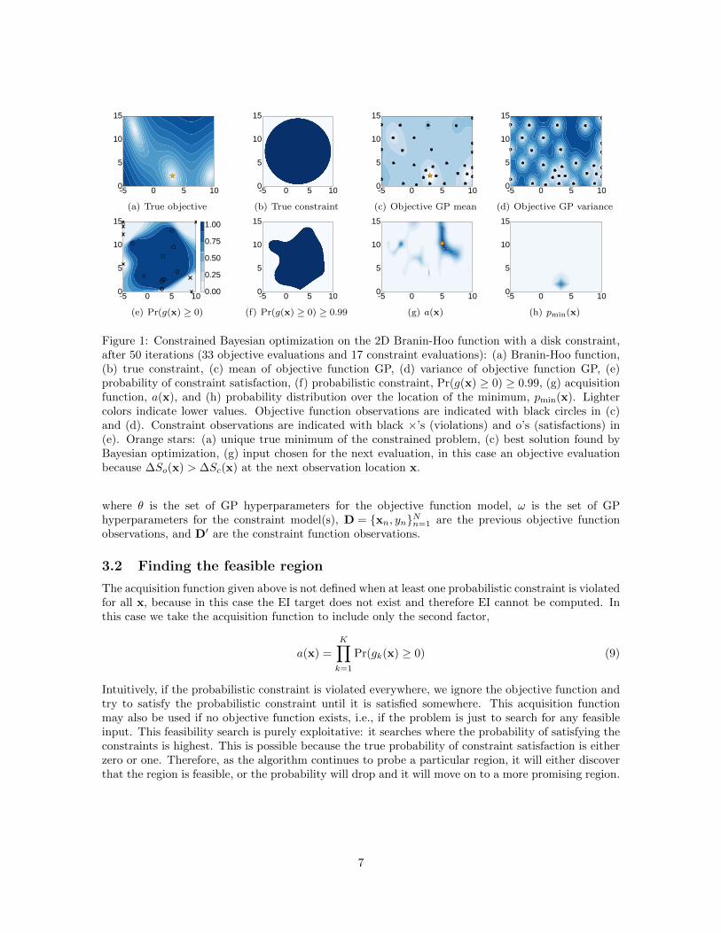
Figure 1: Constrained Bayesian optimization on the 2D Branin-Hoo function with a disk constraint,after 50 iterations (33 objective evaluations and 17 constraint evaluations): (a) Branin-Hoo function,(b) true constraint, (c) mean of objective function GP, (d) variance of objective function GP, (e)probability of constraint satisfaction, (f) probabilistic constraint, Pr(g(x) ≥ 0) ≥ 0.99, (g) acquisitionfunction, a(x), and (h) probability distribution over the location of the minimum, pmin(x). Lightercolors indicate lower values. Objective function observations are indicated with black circles in (c)and (d). Constraint observations are indicated with black ×’s (violations) and o’s (satisfactions) in(e). Orange stars: (a) unique true minimum of the constrained problem, (c) best solution found byBayesian optimization, (g) input chosen for the next evaluation, in this case an objective evaluationbecause ∆So(x) > ∆Sc(x) at the next observation location x.

where θ is the set of GP hyperparameters for the objective function model, ω is the set of GPhyperparameters for the constraint model(s), D = {xn, yn}Nn=1 are the previous objective functionobservations, and D′ are the constraint function observations.

3.2 Finding the feasible region

The acquisition function given above is not defined when at least one probabilistic constraint is violatedfor all x, because in this case the EI target does not exist and therefore EI cannot be computed. Inthis case we take the acquisition function to include only the second factor,

a(x) =

K∏k=1

Pr(gk(x) ≥ 0) (9)

Intuitively, if the probabilistic constraint is violated everywhere, we ignore the objective function andtry to satisfy the probabilistic constraint until it is satisfied somewhere. This acquisition functionmay also be used if no objective function exists, i.e., if the problem is just to search for any feasibleinput. This feasibility search is purely exploitative: it searches where the probability of satisfying theconstraints is highest. This is possible because the true probability of constraint satisfaction is eitherzero or one. Therefore, as the algorithm continues to probe a particular region, it will either discoverthat the region is feasible, or the probability will drop and it will move on to a more promising region.

7

3.3 Acquisition function for decoupled observations

In some problems, the objective and constraint functions may be evaluated independently. We call thisproperty the decoupling of the objective and constraint functions. In decoupled problems, we mustchoose to evaluate either the objective function or one of the constraint functions at each iterationof Bayesian optimization. As discussed in Section 1.3, it is important to identify problems with thisdecoupled structure, because often some of the functions are much more expensive to evaluate thanothers. Bayesian optimization with decoupled constraints is a form of multi-task Bayesian optimization(Swersky et al., 2013), in which the different black-boxes or tasks are the objective and decoupledconstraint(s), represented by the set {objective, 1, 2, . . . ,K} for K constraints.

3.3.1 Chicken and Egg Pathology

One possible acquisition function for decoupled constraints is the expected improvement of individ-ually evaluating each task. However, the myopic nature of the EI criterion causes a pathology inthis formulation that prevents exploration of the design space. Consider a situation, with a singleconstraint, in which some feasible region has been identified and thus the current best input is defined,but a large unexplored region remains. Evaluating only the objective in this region could not causeimprovement as our belief about Pr(g(x) ≥ 0) will follow the prior and not exceed the threshold 1− δ.Likewise, evaluating only the constraint would not cause improvement because our belief about theobjective will follow the prior and is unlikely to become the new best. This is a causality dilemma: wemust learn that both the objective and the constraint are favorable for improvement to occur, but thisis not possible when only a single task is observed. This difficulty suggests a non-myopic aquisitionfunction which assesses the improvement after a sequence of objective and constraint observations.However, such a multi-step acquisition function is intractable in general (Ginsbourger and Riche,2010).

Instead, to address this pathology, we propose to use the coupled acquisition function (Eq. 7) toselect an input x for observation, followed by a second step to determine which task will be evaluatedat x. Following Swersky et al. (2013), we use the entropy search criterion (Hennig and Schuler, 2012)to select a task. However, our framework does not depend on this choice.

3.3.2 Entropy Search Criterion

Entropy search works by considering pmin(x), the probability distribution over the location of theminimum of the objective function. Here, we extend the definition of pmin to be the probability distri-bution over the location of the solution to the constrained problem. Entropy search seeks the actionthat, in expectation, most reduces the relative entropy between pmin(x) and an uninformative basedistribution such as the uniform distribution. Intuitively speaking, we want to reduce our uncertaintyabout pmin as much as possible at each step, or, in other words, maximize our information gain ateach step. Following Hennig and Schuler (2012), we choose b(x) to be the uniform distribution on theinput space. Given this choice, the relative entropy of pmin and b is the differential entropy of pmin upto a constant that does not affect the choice of task. Our decision criterion is then

T ∗ = arg minT

Ey[S(p(yT )min

)− S(pmin)

], (10)

where T is one of the tasks in {objective, 1, 2, . . . ,K}, T ∗ is the selected task, S(·) is the differen-

tial entropy functional, and p(yT )min is pmin conditioned on observing the value yT for task T . When

integrating out the GP covariance hyperparameters, the full form is

T ∗ = arg minT

∫S(p(yT )min

)p (yT |θ, ω) dyT dθ dω (11)

8

10 20 30 40 50

7.5

8

8.5

9

9.5

Function Evaluations

Min

Fun

ctio

n V

alue

Constrained GP EI MCMCGP EI MCMC

(a) Online LDA

20 40 60 80 100

0.1

0.2

0.3

0.4

0.5

0.6

0.7

0.8

Function Evaluations

Min

Fun

ctio

n V

alue

Constrained GP EI MCMCGP EI MCMC

(b) Neural Network

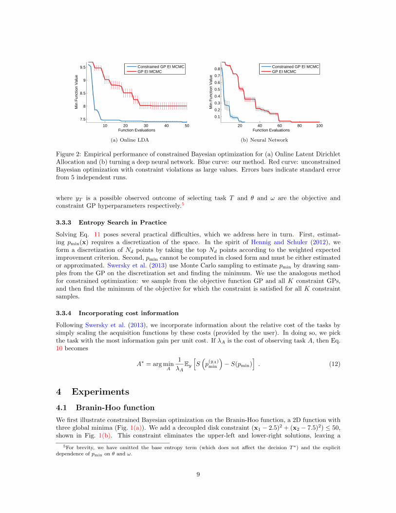
Figure 2: Empirical performance of constrained Bayesian optimization for (a) Online Latent DirichletAllocation and (b) turning a deep neural network. Blue curve: our method. Red curve: unconstrainedBayesian optimization with constraint violations as large values. Errors bars indicate standard errorfrom 5 independent runs.

where yT is a possible observed outcome of selecting task T and θ and ω are the objective andconstraint GP hyperparameters respectively.5

3.3.3 Entropy Search in Practice

Solving Eq. 11 poses several practical difficulties, which we address here in turn. First, estimat-ing pmin(x) requires a discretization of the space. In the spirit of Hennig and Schuler (2012), weform a discretization of Nd points by taking the top Nd points according to the weighted expectedimprovement criterion. Second, pmin cannot be computed in closed form and must be either estimatedor approximated. Swersky et al. (2013) use Monte Carlo sampling to estimate pmin by drawing sam-ples from the GP on the discretization set and finding the minimum. We use the analogous methodfor constrained optimization: we sample from the objective function GP and all K constraint GPs,and then find the minimum of the objective for which the constraint is satisfied for all K constraintsamples.

3.3.4 Incorporating cost information

Following Swersky et al. (2013), we incorporate information about the relative cost of the tasks bysimply scaling the acquisition functions by these costs (provided by the user). In doing so, we pickthe task with the most information gain per unit cost. If λA is the cost of observing task A, then Eq.10 becomes

A∗ = arg minA

1

λAEy[S(p(yA)min

)− S(pmin)

]. (12)

4 Experiments

4.1 Branin-Hoo function

We first illustrate constrained Bayesian optimization on the Branin-Hoo function, a 2D function withthree global minima (Fig. 1(a)). We add a decoupled disk constraint (x1 − 2.5)2 + (x2 − 7.5)2) ≤ 50,shown in Fig. 1(b). This constraint eliminates the upper-left and lower-right solutions, leaving a

5For brevity, we have omitted the base entropy term (which does not affect the decision T ∗) and the explicitdependence of pmin on θ and ω.

9

0 1 2 3 4

log10τ

-3

-2

-1

0lo

g10ε

-5.4-4.8-4.2-3.6-3.0-2.4-1.8-1.2

(a) Objective Function

0 1 2 3 4

log10τ

-3

-2

-1

0

log

10ε

0.00

0.25

0.50

0.75

1.00

(b) Geweke

0 1 2 3 4

log10τ

-3

-2

-1

0

log

10ε

0.00

0.25

0.50

0.75

1.00

(c) Gelman-Rubin

0 1 2 3 4

log10τ

-3

-2

-1

0

log

10ε

0.00

0.25

0.50

0.75

1.00

(d) Stability

0 1 2 3 4

log10τ

-3

-2

-1

0

log

10ε

0.00

0.25

0.50

0.75

1.00

(e) Overall

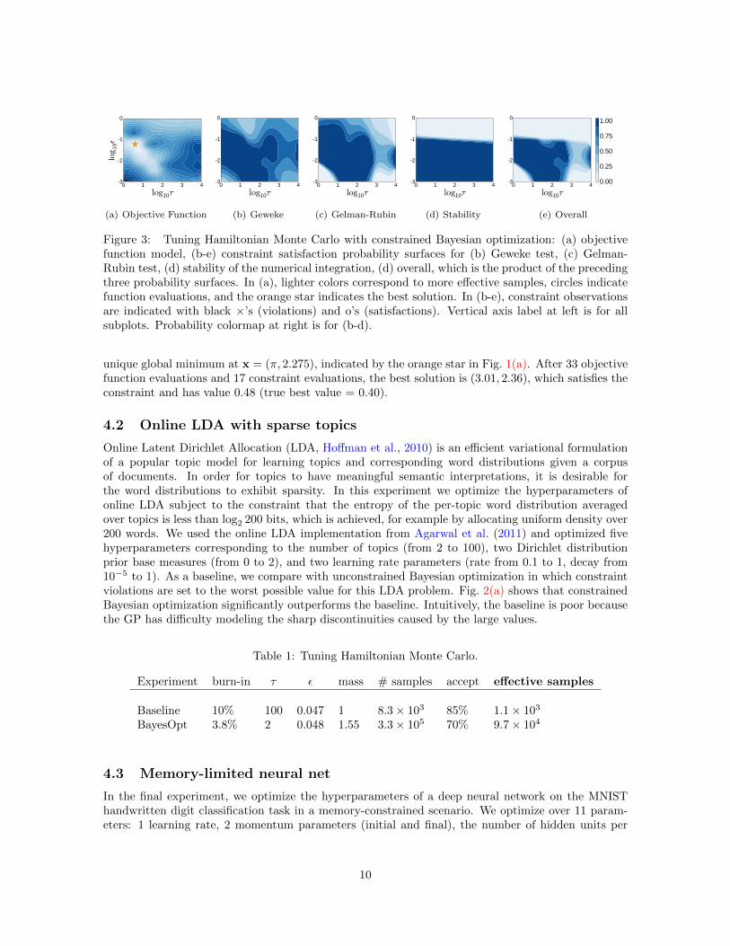
Figure 3: Tuning Hamiltonian Monte Carlo with constrained Bayesian optimization: (a) objectivefunction model, (b-e) constraint satisfaction probability surfaces for (b) Geweke test, (c) Gelman-Rubin test, (d) stability of the numerical integration, (d) overall, which is the product of the precedingthree probability surfaces. In (a), lighter colors correspond to more effective samples, circles indicatefunction evaluations, and the orange star indicates the best solution. In (b-e), constraint observationsare indicated with black ×’s (violations) and o’s (satisfactions). Vertical axis label at left is for allsubplots. Probability colormap at right is for (b-d).

unique global minimum at x = (π, 2.275), indicated by the orange star in Fig. 1(a). After 33 objectivefunction evaluations and 17 constraint evaluations, the best solution is (3.01, 2.36), which satisfies theconstraint and has value 0.48 (true best value = 0.40).

4.2 Online LDA with sparse topics

Online Latent Dirichlet Allocation (LDA, Hoffman et al., 2010) is an efficient variational formulationof a popular topic model for learning topics and corresponding word distributions given a corpusof documents. In order for topics to have meaningful semantic interpretations, it is desirable forthe word distributions to exhibit sparsity. In this experiment we optimize the hyperparameters ofonline LDA subject to the constraint that the entropy of the per-topic word distribution averagedover topics is less than log2 200 bits, which is achieved, for example by allocating uniform density over200 words. We used the online LDA implementation from Agarwal et al. (2011) and optimized fivehyperparameters corresponding to the number of topics (from 2 to 100), two Dirichlet distributionprior base measures (from 0 to 2), and two learning rate parameters (rate from 0.1 to 1, decay from10−5 to 1). As a baseline, we compare with unconstrained Bayesian optimization in which constraintviolations are set to the worst possible value for this LDA problem. Fig. 2(a) shows that constrainedBayesian optimization significantly outperforms the baseline. Intuitively, the baseline is poor becausethe GP has difficulty modeling the sharp discontinuities caused by the large values.

Table 1: Tuning Hamiltonian Monte Carlo.

Experiment burn-in τ ε mass # samples accept effective samples

Baseline 10% 100 0.047 1 8.3× 103 85% 1.1× 103

BayesOpt 3.8% 2 0.048 1.55 3.3× 105 70% 9.7× 104

4.3 Memory-limited neural net

In the final experiment, we optimize the hyperparameters of a deep neural network on the MNISThandwritten digit classification task in a memory-constrained scenario. We optimize over 11 param-eters: 1 learning rate, 2 momentum parameters (initial and final), the number of hidden units per

10

layer (2 layers), the maximum norm on model weights (for 3 sets of weights), and the dropout regu-larization probabilities (for the inputs and 2 hidden layers). We optimize the classification error ona withheld validation set under the constraint that the total number of model parameters (weightsin the network) must be less than one million. This constraint is decoupled from the objective andinexpensive to evaluate, because the number of weights can be calculated directly from the parame-ters, without training the network. We train the neural network using momentum-based stochasticgradient descent which is notoriously difficult to tune as training can diverge under various combina-tions of the momentum and learning rate. When training diverges, the objective function cannot bemeasured. Reporting the constraint violation as a large objective value performs poorly because itintroduces sharp discontinuities that are hard to model (Fig. 2). This necessitates a second noisy, bi-nary constraint which is violated when training diverges, for example when the both the learning rateand momentum are too large. The network is trained6 for 25,000 weight updates and the objectiveis reported as classification error on the standard validation set. Our Bayesian optimization routinecan thus choose between two decoupled tasks, evaluating the memory constraint or the validationerror after a full training run. Evaluating the validation error can still cause a constraint violationwhen the training diverges, which is treated as a binary constraint in our model. Fig. 2(b) shows acomparison of our constrained Bayesian optimization against a baseline standard Bayesian optimiza-tion where constraint violations are treated as resulting in a random classifier (90% error). Only theobjective evaluations are presented, since constraint evaluations are extremely inexpensive comparedto an entire training run. In the event that training diverges on an objective evaluation, we report90% error. The optimized net has a learning rate of 0.1, dropout probabilities of 0.17 (inputs), 0.30(first layer), and 0 (second layer), initial momentum 0.86, and final momentum 0.81. Interestingly,the optimization chooses a small first layer (size 312) and a large second layer (size 1772).

4.4 Tuning Markov chain Monte Carlo

Hamiltonian Monte Carlo (HMC) is a popular MCMC sampling technique that takes advantage ofgradient information for rapid mixing. However, HMC contains several parameters that require carefultuning. The two basic parameters are the number of leapfrog steps τ , and the step size ε. HMCmay also include a mass matrix which introduces O(D2) additional parameters in D dimensions,although the matrix is often chosen to be diagonal (D parameters) or a multiple of the identitymatrix (1 parameter) (Neal, 2011). In this experiment, we optimize the performance of HMC usingBayesian optimization; see Mahendran et al. (2012) for a similar approach. We optimize the followingparameters: τ , ε, a mass parameter, and the fraction of the allotted computation time spent burningin the chain.

Our experiment measures the number of effective samples (ES) in a fixed computation time; thiscorresponds to finding chains that minimize estimator variance. We impose the constraints that thegenerated samples must pass the Geweke (Geweke, 1992) and Gelman-Rubin (Gelman and Rubin,1992) convergence diagnostics. In particular, we require the worst (largest absolute value) Geweketest score across all variables and chains to be at most 2.0, and the worst (largest) Gelman-Rubinscore between chains and across all variables to be at most 1.2. We use PyMC (Patil et al., 2010)for the convergence diagnostics and the LaplacesDemon R package to compute effective sample size.The chosen thresholds for the convergence diagnostics are based on the PyMC and LaplacesDemondocumentation. The HMC integration may also diverge for large values of ε; we treat this as anadditional constraint, and set δ = 0.05 for all constraints. We optimize HMC sampling from theposterior of a logistic regression binary classification problem using the German credit data set fromthe UCI repository (Frank and Asuncion, 2010). The data set contains 1000 data points, and isnormalized to have unit variance. We initialize each chain randomly with D independent draws froma Gaussian distribution with mean zero and standard deviation 10−3. For each set of inputs, wecompute two chains, each with 5 minutes of computation time on a single core of a compute node.

6We use the Deepnet package: https://github.com/nitishsrivastava/deepnet.

11

Fig. 3 shows the constraint surfaces discovered by Bayesian optimization for a simpler experimentin which only τ and ε are varied; burn-in is fixed at 10% and the mass is fixed at 1. These diagramsyield interpretations of the feasible region; for example, Fig. 3(d) shows that the numerical integrationdiverges for values of ε above ≈ 10−1. Table 1 shows the results of our 4-parameter optimization after50 iterations, compared with a baseline that is reflective of a typical HMC configuration: 10% burnin, 100 leapfrog steps, and the step size chosen to yield an 85% proposal accept rate. Each row in thetable was produced by averaging 5 independent runs with the given parameters. The optimizationchooses to perform very few (τ = 2) leapfrog steps and spend relatively little time (3.8%) burning inthe chain, and chooses an acceptance rate of 70%. In contrast, the baseline spends much more timegenerating each proposal (τ = 100), which produces many fewer total samples and, correspondingly,significantly fewer effective samples.

5 Conclusion

In this paper we extended Bayesian optimization to constrained optimization problems. Becauseconstraint observations may be noisy, we formulate the problem using probabilistic constraints, al-lowing the user to directly express the tradeoff between cost and risk by specifying the confidenceparameter δ. We then propose an acquisition function to perform constrained Bayesian optimization,including the case where the objective and constraint(s) may be observed independently. We demon-strate the effectiveness of our system on the meta-optimization of machine learning algorithms andsampling techniques. Constrained optimization is a ubiquitous problem and we believe this work hasapplications in areas such as product design (e.g. designing a low-calorie cookie), machine learningmeta-optimization (as in our experiments), real-time systems (such as a speech recognition system ona mobile device with speed, memory, and/or energy usage constraints), or any optimization problemin which the objective function and/or constraints are expensive to evaluate and possibly noisy.

Acknowledgements

The authors would like to thank Geoffrey Hinton, George Dahl, and Oren Rippel for helpful dis-cussions, and Robert Nishihara for help with the experiments. This work was partially funded byDARPA Young Faculty Award N66001-12-1-4219. Jasper Snoek is a fellow in the Harvard Center forResearch on Computation and Society.

References

Alekh Agarwal, Olivier Chapelle, Miroslav Dudık, and John Langford. A reliable effective terascalelinear learning system, 2011. arXiv: 1110.4198 [cs.LG].

James S. Bergstra, Remi Bardenet, Yoshua Bengio, and Balazs Kegl. Algorithms for hyper-parameteroptimization. In NIPS. 2011.

Eric Brochu, Tyson Brochu, and Nando de Freitas. A Bayesian interactive optimization approach toprocedural animation design. In ACM SIGGRAPH/Eurographics Symposium on Computer Anima-tion, 2010a.

Eric Brochu, Vlad M. Cora, and Nando de Freitas. A tutorial on Bayesian optimization of expensivecost functions, 2010b. arXiv:1012.2599 [cs.LG].

Adam D. Bull. Convergence rates of efficient global optimization algorithms. JMLR, (3-4):2879–2904,2011.

Nando de Freitas, Alex Smola, and Masrour Zoghi. Exponential regret bounds for Gaussian processbandits with deterministic observations. In ICML, 2012.

12

Josip Djolonga, Andreas Krause, and Volkan Cevher. High dimensional Gaussian Process bandits. InNIPS, 2013.

Andrew Frank and Arthur Asuncion. UCI machine learning repository, 2010.

Andrew Gelman and Donald R. Rubin. A single series from the Gibbs sampler provides a false senseof security. In Bayesian Statistics, pages 625–32. Oxford University Press, 1992.

John Geweke. Evaluating the accuracy of sampling-based approaches to the calculation of posteriormoments. In Bayesian Statistics, pages 169–193. University Press, 1992.

David Ginsbourger and Rodolphe Riche. Towards Gaussian process-based optimization with finitetime horizon. In Advances in Model-Oriented Design and Analysis. Physica-Verlag HD, 2010.

Robert B. Gramacy and Herbert K. H. Lee. Optimization under unknown constraints, 2010.arXiv:1004.4027 [stat.ME].

Philipp Hennig and Christian J. Schuler. Entropy search for information-efficient global optimization.JMLR, 13, 2012.

Matthew Hoffman, David M. Blei, and Francis Bach. Online learning for latent Dirichlet allocation.In NIPS, 2010.

Frank Hutter, Holger H. Hoos, and Kevin Leyton-Brown. Sequential model-based optimization forgeneral algorithm configuration. In LION, 2011.

Donald R. Jones. A taxonomy of global optimization methods based on response surfaces. Journal ofGlobal Optimization, 21, 2001.

Andreas Krause and Cheng Soon Ong. Contextual Gaussian Process bandit optimization. In NIPS,2011.

Dan Lizotte. Practical Bayesian Optimization. PhD thesis, University of Alberta, Edmonton, Alberta,2008.

Nimalan Mahendran, Ziyu Wang, Firas Hamze, and Nando de Freitas. Adaptive MCMC with Bayesianoptimization. In AISTATS, 2012.

Jonas Mockus, Vytautas Tiesis, and Antanas Zilinskas. The application of Bayesian methods forseeking the extremum. Towards Global Optimization, 2, 1978.

Iain Murray and Ryan P. Adams. Slice sampling covariance hyperparameters of latent Gaussianmodels. In NIPS, 2010.

Iain Murray, Ryan P. Adams, and David J.C. MacKay. Elliptical slice sampling. JMLR, 9:541–548,2010.

Radford Neal. Slice sampling. Annals of Statistics, 31:705–767, 2000.

Radford Neal. MCMC using Hamiltonian dynamics. In Handbook of Markov Chain Monte Carlo.Chapman and Hall/CRC, 2011.

Anand Patil, David Huard, and Christopher Fonnesbeck. PyMC: Bayesian stochastic modelling inPython. Journal of Statistical Software, 2010.

Carl Rasmussen and Christopher Williams. Gaussian Processes for Machine Learning. MIT Press,2006.

13

A. Shapiro, D. Dentcheva, and A. Ruszczynski. Lectures on stochastic programming: modeling andtheory. MPS-SIAM Series on Optimization, Philadelphia, USA, 2009.

Jasper Snoek. Bayesian Optimization and Semiparametric Models with Applications to AssistiveTechnology. PhD thesis, University of Toronto, Toronto, Canada, 2013.

Jasper Snoek, Hugo Larochelle, and Ryan P. Adams. Practical Bayesian optimization of machinelearning algorithms. In NIPS, 2012.

Niranjan Srinivas, Andreas Krause, Sham Kakade, and Matthias Seeger. Gaussian process optimiza-tion in the bandit setting: no regret and experimental design. In ICML, 2010.

Kevin Swersky, Jasper Snoek, and Ryan P. Adams. Multi-task Bayesian optimization. In NIPS, 2013.

Ziyu Wang, Masrour Zoghi, Frank Hutter, David Matheson, and Nando de Freitas. Bayesian opti-mization in high dimensions via random embeddings. In IJCAI, 2013.

Marcela Zuluaga, Andreas Krause, Guillaume Sergent, and Markus Puschel. Active learning formulti-objective optimization. In ICML, 2013.

14