Bayesian Object Localisation in Images - Temple …latecki/Courses/RobotFall07/PapersFall07...Bayesian Object Localisation in Images ... that has undergone certain distortions

International Journal of Computer Vision 44(2), 111–135, 2001c© 2001 Kluwer Academic Publishers. Manufactured in The Netherlands.

Bayesian Object Localisation in Images

J. SULLIVAN, A. BLAKE,* M. ISARD, AND J. MACCORMICKDepartment of Engineering Science, University of Oxford, Parks Road Oxford OX1 3PJ, UK

Web: http://www.robots.ox.ac.uk/∼vdg/

Received August 6, 1999; Revised January 31, 2001; Accepted April 2, 2001

Abstract. A Bayesian approach to intensity-based object localisation is presented that employs a learned proba-bilistic model of image filter-bank output, applied via Monte Carlo methods, to escape the inefficiency of exhaustivesearch.

An adequate probabilistic account of image data requires intensities both in the foreground (i.e. over the object),and in the background, to be modelled. Some previous approaches to object localisation by Monte Carlo methods haveused models which, we claim, do not fully address the issue of the statistical independence of image intensities. It isaddressed here by applying to each image a bank of filters whose outputs are approximately statistically independent.Distributions of the responses of individual filters, over foreground and background, are learned from training data.These distributions are then used to define a joint distribution for the output of the filter bank, conditioned on objectconfiguration, and this serves as an observation likelihood for use in probabilistic inference about localisation.

The effectiveness of probabilistic object localisation in image clutter, using Bayesian Localisation, is illustrated.Because it is a Monte Carlo method, it produces not simply a single estimate of object configuration, but anentire sample from the posterior distribution for the configuration. This makes sequential inference of configurationpossible. Two examples are illustrated here: coarse to fine scale inference, and propagation of configuration estimatesover time, in image sequences.

Keywords: vision, object location, Monte Carlo, filter-bank, statistical independence

1. Introduction

The paper develops a Bayesian approach to localisingobjects in images. Approximate probabilistic inferenceof object location is done using a learned likelihood forthe output of a bank of image filters. The new approachis termed Bayesian Localisation.1

Following the framework of “pattern theory”(Grenander, 1981; Mumford, 1996), an image is an in-tensity function I (x), x ∈ D ⊂ R2, taken to containa template T (x) that has undergone certain distortions.Much of the distortion is accounted for as a warp ofthe template T (x) into an intermediate image I by an

*Present address: Microsoft Research, 1 Guildhall Street,Cambridge, UK.

(inverse) warp mapping gX :

T (x) = I (gX (x)), x ∈ S, (1)

where S is the domain of T , and gX is parameterised byX ∈ X over some configuration space X (for instanceplanar affine warps). The remainder of the distortionin the process of image formation, is taken to have theform of a random process applied pointwise to intensityvalues in I , to produce the final image I :

I (x) = f ( I (x), x, w(x)), (2)

where w is a noise process and f is a function that maybe nonlinear. Note that (2) may include a component ofsensor noise but in practice, this is emphatically not its

112 Sullivan et al.

principal role. Camera sensor noise is negligible com-pared with the principal source of variability that needsto be modelled probabilistically: illumination changes,and the residual variability between objects of a givenclass that is unmodelled otherwise.

Analysis “by synthesis” then consists of theBayesian construction of a posterior distribution for X .That is, given a prior distribution2 p0(X) for the con-figuration X , and an observation likelihood L(X) =p(Z | X) where Z ≡ Z(I ) is some finite-dimensionalrepresentation of the image I , the posterior density forX is given by

p(X | Z) ∝ p0(X)p(Z | X). (3)

In the straightforward case of normal distributions, (3)can be computed in closed form, and this can be effec-tive in the fusion of visual data (Matthies et al., 1989;Szeliski, 1990). In the non-Gaussian cases commonlyarising, for example in image clutter or with multiplemodels, sampling methods are effective (Geman andGeman, 1984; Gelfand and Smith, 1990; Grenanderet al., 1991), and that is what we use here.

There have been a number of powerful demonstra-tions in the pattern theory genre, especially in thefield of face analysis (Cootes et al., 1995; Beymer andPoggio, 1995; Vetter and Poggio, 1996) and in biologi-cal images (Grenander and Miller, 1994; Storvik, 1994;Ripley, 1992). A great attraction of pattern theoretic al-gorithms is that they can potentially generate not just

Table 1. Precursors to Bayesian localisation.

IB FL MS PD BM SI Comments

Burt (1983) × × multi-scale pyramid

Witkin et al. (1987); Scharstein × × scale-space matchingand Szeliski (1998)

Grenander et al. (1991); × × × random diffeomorphismsRipley (1992)

Viola and Wells (1993) × × mutual information

Cootes et al. (1995) × × × multi-scale active contours

Black and Yacoob (1995); × × affine flow/warpBascle and Deriche (1995);Hager and Toyama (1996)

Isard and Blake (1996) × × random, time-varying active contours

Olshausen and Field (1996); × × × independent components (ICA)Bell and Sejnowski (1997)

Geman and Jedynak (1996) × × × response learning

a single estimate of object configuration, but an en-tire probability distribution. This facilitates sequentialinference, across spatial scales, across time for imagesequence analysis, and even across sensory modalities.

The previous work most closely related to Bayesianlocalisation is as follows. First Grenander et al. (1991)use randomly generated diffeomorphisms as a mech-anism for Bayesian inference of contour shape. Itsdrawback is that it treats the intensities of individ-ual, neighbouring pixels as independent which leads tounrealistic observation likelihood models. Second, thealgorithm of Viola and Wells (1995) for registrationby maximisation of mutual information contains thekey elements of probabilistic modelling and learningof foreground, but does not take account of back-ground statistics. It computes a single estimate ofobject pose, rather than sampling the entire distri-bution of the posterior. Thirdly, Geman and Jedynak(1996) use probabilistic foreground/background learn-ing for road tracking but compute only a single esti-mate of pose rather than sampling from the posterior;furthermore, the statistical independence of observa-tions, which is a necessary assumption of the method,is not investigated. Attributes of these and other impor-tant prior work are summarised in Table 1, in terms ofelements of Bayesian Localisation as follows.

IB Intensity Based observations, not just edges.FL Foreground Learning in terms of probability dis-

tributions estimated from one or more trainingexamples.

Bayesian Object Localisation in Images 113

MS Multiple Scale search is well known to be a soundbasis for efficient image-search.

PD Posterior Distributions are generated, rather thanjust single estimates, facilitating sequential rea-soning for image sequence analysis, and poten-tially across sensory modalities.

BM Background Modelling: in a valid Bayesian anal-ysis, image observations Z must be regarded asfixed, not as a function Z(X) of a hypothesis X .For example, a sum-squared difference measureviolates this principle by considering only theportion of an image directly under a given tem-plate T (x). In contrast, in a Bayesian approach,evidence about where the object is not must betaken into account, and that requires a probabilis-tic model of the image background.

SI Statistical Independence of observations must beunderstood if constructed observation likelihoodsare to be valid.

2. Bayesian Framework

2.1. Image Observations

Image observations can be based on edges or on in-tensities (and a combination of the two can be particu-larly effective (Bascle and Deriche, 1995)). Edges areattractive because of their superior invariance to vari-ations in illumination and other perturbations, but trueBayesian inference (3) with edges is not feasible. Thisis because, given a set Z of all edges in an image, thereis no known construction for the observation densityp(Z | X) that is probabilistically consistent. One fea-sible approach allows Z to be a function of X , so thatZ(X) consists solely of those edges found close to theoutline of the object, in configuration X . Then a likeli-hood L(X) = p(Z(X) | X) can be constructed (Isardand Blake, 1998), but cannot be used for true Bayesianinference as that demands that the observations Z mustbe fixed, not a function of X . The alternative approachfollowed here avoids the problem encountered withedges by using a fixed set of intensities covering theentire image. turns out that Bayesian localisation sub-sumes the need for explicit edge features, because itsprobabilistic model of intensity naturally captures fore-ground/background transitions.

2.2. Sum-Squared Difference and Cross-Correlation

One approach to interpreting image intensities proba-bilistically is to make the very special assumption that

image distortions are due to additive white noise. Then,a likelihood

L(X) = exp −�(X) (4)

can be defined (Szeliski, 1990) in terms of a sum-squared difference (SSD) function �(X):

�(X) =∫

x∈Sw(x)(T (x) − I (gX (x)))2, (5)

where the weighting w(x) depends on the noise vari-ance. It is worth noting that a likelihood such as (4)is generally multi-modal, having many maxima. Inge-nious algorithms (Witkin et al., 1987; Scharstein andSzeliski, 1998) have been needed to find maximumlikelihood estimates. Multi-modality is a feature of im-age likelihood functions generally, whether based onedges or intensities, and is the reason for needing ran-dom sampling methods later in this paper.

The likelihood (4) has been used successfully in sur-face reconstruction (Szeliski, 1990) but is not appropri-ate for image intensity modelling, for two reasons. Thefirst is that the assumption of additive, white noise is notplausible. It implies statistical independence of adja-cent pixels. In practice however, the sources of intensityvariation are illumination changes and intrinsic vari-ability between objects of one class. Such variationsare spatially correlated (Belhumeur and Kriegman,1998). If a fine-scale independence assumption is madenonetheless, the resulting likelihood function L(X)

can have grossly exaggerated variations (Ripley, 1992),even as great as several hundred orders of magnitude,for minor perturbations of X .

The second reason is that the SSD-based likelihood(5) L(X) depends on the image intensities over a do-main gX (S) that varies with X . This means, effectively,that the observation likelihood is L(X) = p(Z(X) | X),depending on observations Z(X) which are not fixed.This was precisely the problem with edge-based ob-servations which we set out to put right! The problemcan be rectified by insisting that observations Z arecomputed as some fixed function of an image I (x),x ∈ D, where D is a fixed domain, irrespective of X .The domain D will then be the union of a foreground re-gion gX (S) ∩ D, and a background region D\{gX (S)}.Any consistently constructed likelihood p(Z | X) musttherefore depend both on the foreground and on thestatistics of the background. The intuition behind thisis that the image contains statistical information bothabout where the object is and where it is not. A complete

114 Sullivan et al.

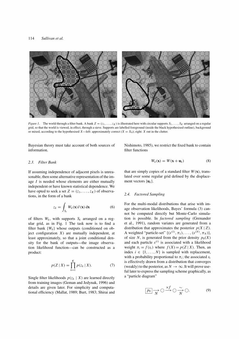
Figure 1. The world through a filter bank. A bank Z = (z1, . . . , zK ) is illustrated here with circular supports S1, . . . , SK arranged on a regulargrid, so that the world is viewed, in effect, through a sieve. Supports are labelled foreground (inside the black hypothesised outline), backgroundor mixed, according to the hypothesised X—left: approximately correct (X = X0); right: X out in the clutter.

Bayesian theory must take account of both sources ofinformation.

2.3. Filter Bank

If assuming independence of adjacent pixels is unrea-sonable, then some alternative representation of the im-age I is needed whose elements are either mutuallyindependent or have known statistical dependence. Wehave opted to seek a set Z = (z1, . . . , zK ) of observa-tions, in the form of a bank

zk =∫

Sk

Wk(x)I (x) dx (6)

of filters Wk , with supports Sk arranged on a reg-ular grid, as in Fig. 1 The task now is to find afilter bank {Wk} whose outputs (conditioned on ob-ject configuration X ) are mutually independent, atleast approximately, so that a joint conditional den-sity for the bank of outputs—the image observa-tion likelihood function—can be constructed as aproduct:

p(Z | X) =K∏

k=1

p(zk | X). (7)

Single filter likelihoods p(zk | X) are learned directlyfrom training images (Geman and Jedynak, 1996) anddetails are given later. For simplicity and computa-tional efficiency (Mallat, 1989; Burt, 1983; Shirai and

Nishimoto, 1985), we restrict the fixed bank to containfilter functions

Wk(x) = W (x + uk) (8)

that are simply copies of a standard filter W (x), trans-lated over some regular grid defined by the displace-ment vectors {uk}.

2.4. Factored Sampling

For the multi-modal distributions that arise with im-age observation likelihoods, Bayes’ formula (3) can-not be computed directly but Monte-Carlo simula-tion is possible. In factored sampling (Grenanderet al., 1991), random variates are generated from adistribution that approximates the posterior p(X | Z).A weighted “particle-set” {(s(1), π1), . . . , (s(N ), πN )},of size N , is generated from the prior density p0(X)

and each particle s(i) is associated with a likelihoodweight πi = f (si ) where f (X) = p(Z | X). Then, anindex i ∈ {1, . . . , N } is sampled with replacement,with a probability proportional to πi ; the associated si

is effectively drawn from a distribution that converges(weakly) to the posterior, as N → ∞. It will prove use-ful later to express the sampling scheme graphically, asa “particle diagram”

p0 −→N

© ×f−→ © ∼−→N

©. (9)


Figure 2. The support of a mask. A circular support set S is illustrated here, split into subsets F(X) from the foreground and B(X) from thebackground.

It is interpreted as follows: the first arrow denotesdrawing N particles from a known density p0, withequal weights πi = 1/N . (Particle sets are representedby open circles.) The ×f operation denotes likelihoodweighting of a particle set:

πi → f(s(i)

)πi , i = 1, . . . , N .

The final step denotes sampling with replacement, asdescribed above, repeated N times, to form a new setof size N in which each particle is given a unit weight;each particle is therefore drawn approximately fromthe posterior.

Where the likelihood f is a very narrow function inconfiguration space, sampling can become inefficient,requiring large N in order to give reasonable estimatesof the posterior. In the paper (section 8) it is shown howthis can be mitigated by “layered sampling” in whichbroader likelihood functions are used in an advisorycapacity to “focus” the particle set down, in stages. Inthe vision context, layered sampling is a vehicle forimplementing multi-scale processing.

3. Probabilistic Modelling of Observations

The observation (i.e., output value) z from an individualfilter is generated by integration over a support-set Ssuch as the circular one in Fig. 2, which is generallycomposed of both a background component B(X), anda foreground component F(X):

z | X =∫

B(X)

W (x)I (x) dx︸︷︷︸MAIN NOISE SOURCE

+∫

F(X)

W (x)I (x) dx.

(10)

The main source of variation in z | X is expected tocome from the background which is assumed to be asample from some general class of scenes. In contrast,the foreground relates to a given object, relatively pre-cisely known, though still subject to some variability.This means that there should be a steady reduction inthe variance of the distribution of z | X as X changesfrom values in which the circular support is entirelyover foreground, via intermediate locations overlap-ping both foreground and background, and finally tovalues in which it is entirely over background. This issupported by experiments in which density functionsfor z which have been learned from images, both frombackground regions and also from foreground regions(Fig. 3). The filter used in the experiment is a Gaussian

Gσ (x) = 1

σ 2exp − |x|2

2σ 2(11)

in a circular support of radius r (= 3σ).The role of p(z | X) in Bayesian localisation is as a

likelihood function for X , associated with a particular

Figure 3. Learned observation densities for a Gaussian filter. Den-sities p(z) are exhibited both for foreground and background, in thecase that W (x) is Gaussian, with support radius r = 20 pixels. Unitsof z are intensity, scaled so that intensities in the original image liein the range 0, 1.

116 Sullivan et al.

Figure 4. Observation likelihood. The density p(z | X) is formally a function of z with X as a parameter, and is illustrated for foregroundand background cases. The whole family of such one-dimensional densities, indexed by the continuous variable X , are assembled to synthesisep(z | X), as shown. Now p(z | X) is “sliced” in the orthogonal direction, to generate likelihoods (functions of X for fixed z). In the examples,an observation z = 2 biases X towards a foreground value, whereas z = −1 biases towards background.

observation z, as illustrated in Fig. 4. Note that, al-though X is generally multidimensional, in the dia-gram it is depicted as a one-dimensional variable, forthe sake of clarity. The entire family of idealised den-sities can be represented in (z, X)-space as shown inthe figure. Then, to construct the likelihood functions,the z-value is considered to be fixed and X allowedto vary. This is illustrated in Fig. 4 by consideringslices of constant z. For example, z = 2 in the fig-ure depicts a relative high value which, in the ex-ample, is more likely to be associated with a filter-support lying predominantly over the foreground. Theresulting likelihood is peaked around a value of X cor-responding to predominant foreground support. Con-versely, for z = −1, the support is more likely tobe predominantly over the background and the modeof the likelihood shifts towards background valuesof X .3

Likelihood functions from several observations zk

should “fuse” when they are combined (7), to form ajoint likelihood that is more acutely tuned (Fig. 5) thanthe likelihood for any individual zk . Note the impor-tance of the zk from “mixed” supports, lying partly onthe background and partly on the foreground. It might

be tempting to regard them as contaminated and dis-card them whereas, in fact, they should be especiallyinformative, responding selectively to the boundary ofthe object—see Fig. 1.

Figure 5. “Hyperacuity” from pooled observations. Likelihoodsfrom independent observations combine multiplicatively, to give ajoint likelihood narrower than any of the individual constituents.


Figure 6. Approximating foreground/background supports. Assuming that the object’s bounding contour is sufficiently smooth (on the scaler of the radius of the filter support) the boundary between foreground and background can be approximated as a straight line. The supporttherefore divides into segments with offsets 2rρ and 2r(1 − ρ) for background and foreground respectively.

4. Filter Response-Learning

If it were not for mixed supports, learning would berelatively straightforward. Over the background, forinstance, it would be sufficient just to evaluate the out-puts z (6) of the circular filter repeatedly, at assortedlocations over some training image, and fit a proba-bility distribution pB(z). However, over a mixed sup-port, only a part of the circle lies over the background.If this part is approximated as a segment of a circle(Fig. 6), and provided each filter functional Wk(x) isisotropic (or steerable (Perona, 1992)), then the back-ground distribution can be parameterised by a singleoffset parameter ρ (at a given scale r ). This parameteris defined for 0 ≤ ρ ≤ 1, as in the figure so that: whenρ = 1 the filter support is entirely over the background;when ρ = 0 it is entirely over the foreground; and for0 < ρ < 1 it straddles the object boundary.

Training examples for background learning mustbe constructed over circular segments with offsetsthroughout the range 0 ≤ ρ ≤ 1, to learn backgrounddistributions pB

k (z | ρ). (Clearly, in practice, only a fi-nite number of these can be learned, leaving the contin-uum of ρ to be filled in by interpolation.) To considera hypothesised configuration X , the Bayesian locali-sation algorithm needs to evaluate, for each k, an off-set function ρk(X) and a likelihood pk(z | ρk(X)). Thelikelihood function consists of a sum of background andforeground components, and is therefore constructed asa (numerically approximated) convolution

pk(z | ρ) = pBk (z | ρ) ∗ pF

k (z | ρ) (12)

of learned background and foreground density fun-ctions.

5. Learning the Background Likelihood

Statistical independence of image features is an issuethat has been studied elsewhere, in the context of neu-ral coding (Field, 1987): if neural codes are efficientin the sense of avoiding redundancy, their componentscan be expected to be nearly statistically independent.It is also known that independent components of nat-ural scenes tend to have “sparse” or “hyper-kurtotic”distributions—ones with extended tails compared withthose of a normal distribution (Bell and Sejnowski,1997).

5.1. Experiments with Response Correlation

Experiments on background correlation are done hereusing statistics collected from each of the four scenesin Fig. 7. Our experiments are similar to those doneby Zhu and Mumford (1997) in which they showedthe background distribution is remarkably consistentacross scenes, for a ∇G filter. Here we look at the divof that filter output, which should therefore similarlyshow a consistent distribution, and the small-scale ex-periments done here support that. A necessary condi-tion for independence is freedom from correlation, soautocorrelation was estimated by random sampling ofpairs of supports, separated by a varying displacement.This was done for two choices of filter function W (x):Gaussian G(x) and Laplacian of Gaussian ∇2G(x), andtypical results are shown in Fig. 8. At a displacementsuch as r (= 3σ ), corresponding to a typical separa-tion between filters, the G(x) filter shows correlationand hence there cannot be independence. On the otherhand ∇2G(x) is uncorrelated at a displacement of r .Further experiments, looking at the entire joint distri-bution for responses zk, zl of two filters with variable

118 Sullivan et al.

Figure 7. Background learning: training scenes used in experiments.

Figure 8. Autocorrelation of filter output. Results are for the first (hand) image from Fig. 7, at two sizes of spatial scale r . The Gaussian filterG(x) shows substantial long-range correlation whereas, for ∇2G(x) correlation falls to zero for non-overlapping supports.


Figure 9. Independence of filter output. Two filters displaced δ apart have outputs z1, z2, and the distribution of the difference �z = z1 − z2

is plotted here. The dashed curve shows a reference distribution for large δ. In the case δ = 5 pixels that correlation is high (see Fig. 8) z1, z2

are clearly not independent—the distribution for �z does not match the reference distribution. However with δ = 20 pixels, for which z1, z2

are uncorrelated, they are shown here also to be approximately independent.

spatial separation, support statistical independence, asFig. 9 shows.

The independence is obtained at the cost of throwingaway information about mean response and the 1st mo-ment, though this is likely to be beneficial in conferringsome invariance to illumination variations. These ex-periments were for complete, circular supports. Withpart-segments of a circle (ρ < 1), statistical indepen-dence of ∇2G(x) responses deteriorates. Experimentslike the ones in Fig. 8 show correlation lengths increas-ing for ρ < 1, with ρ = 1

4 the worst case. This will meangreater statistical dependence between mixed supports,and it is not clear how this could be improved; but noteat least that typically it is a minority of filter supportsthat are mixed.

Fitting the Background Distribution. A further ben-efit of the ∇2G(x) filter is that the learned backgrounddistributions turn out to be far more constant across

Figure 10. Learned background distributions. Learned densities pB(z) are shown here for each of the four scenes in Fig. 7 at scale r = 20:they are highly variable for the G(x) filter, but rather consistent for ∇2G(x).

scenes (and this is known to be true also for ∇G fil-ters (Zhu and Mumford, 1997)) than for a plain G(x)

filter. Background distributions were learned by re-peated sampling of zk (6) for randomly positionedsupports, then histogramming and smoothing to esti-mate pB(z). The results for complete circular supports(ρ = 1), shown in Fig. 10, show sufficient consistencyto indicate that some fixed parametric form should besufficient to represent the densities. The learned re-sponses turn out not to be normally distributed, but havea hyper-kurtotic distribution, that is one with greaterkurtosis than a normal distribution, and this is clearlyvisible in the extended tails in Fig. 10. Hyper-kurtoticdistributions are known to emerge in independent com-ponents of images (Bell and Sejnowski, 1997), and areoften found to be well modelled by a single-exponentialdistribution.4

pB(z) ∝ exp − | z | /λ. (13)

120 Sullivan et al.

Figure 11. Exponential model for background distributions. Learned densities pB(z) for the first and last of the 4 scenes in Fig. 7, at scaler = 20 with ρ = 1, are fitted here (by MLE) to an exponential distribution, which captures the elongation of the tails.

The distribution fits the experimental data quite well(Fig. 11). In that case, a global background likelihoodof the form (7), is a product of exponentials of filterresponses, just the scene model derived by Zhu et al.via maximum entropy (Zhu et al., 1998, Eq. (21)).

For ρ < 1 (circle segments), the single-exponentialdistribution does not fit so well, with ρ = 1

4 again beingthe worst case. [This is to be expected, given that ∇2Gdoes not sum to 0 over an arbitrary segment of a circle,except for the semi-circle ρ = 1

2 . This implies that thedistribution mean will not be zero, and hence cannothave single-exponential form.]

Since W = ∇2G sums to 0, the means of densitiespF and pB for foreground and background will alsocoincide at 0, as in Fig. 12. Given this loss of the in-formation associated with the means of pB and pF ,discriminability between foreground and backgroundis reduced, the price paid for improved illumination-invariance. However, the foreground model can beextended in certain ways to improve discriminabil-ity again. One way is “foreground subdivision” as inSection 6; another uses intensity templates (Sullivanand Blake, 2000).

Figure 12. Foreground and background distributions when∫W (x)dx = 0, for support radius r = 20 pixels. The means

of the foreground and background distributions now coincide, cf.Fig. 3.

5.2. Optimal Filter Bank Grid

At a given spatial scale, the maximum informationabout an image can be collected by packing filter sup-ports Sk as densely as possible, within the constraintthat filter outputs zk must be uncorrelated. For filtersWk that are isotropic, correlation depends simply on thedisplacement between pairs of filters. A useful measureis that the correlation function (Fig. 8) crosses 0 at adisplacement of around r (= 3σ ). The most effectivepacking of filters, for the given level of correlation,will be the one that maximises the packing density fora given minimum displacement between filter centres.This is well-known to be a hexagonal tesselation, whosepacking density is approximately 50% greater thansquare packing. For the ∇2G filter, the filter supportis circular5 with radius approximately r (= 3σ ) whichis also the displacement for (approximately) zero cor-relation. Hence supports in the hexagonally tesselatedoptimal filter bank overlap substantially as in Fig. 13.

6. Learning the Foreground Likelihood

Learning distributions for foreground responses is sim-ilar to the background case. As before, pF (z | ρ) islearned for some finite set of ρ-values, and interpolatedfor ρ ∈ [0, 1]. There are some important differenceshowever.

6.1. Deformations and Pooling

Three-dimensional transformations and deformationsof the foreground object must be taken into ac-count. Tabulating pF not only against ρ but alsoagainst transformation parameters is computationally


Figure 13. Optimal tesselation of filter supports. Maximum den-sity of ∇2G filters, while avoiding correlation between filter pairs,is achieved by a hexagonal tesselation, as shown, with substantialoverlap (support radius r = 40 pixels illustrated).

infeasible. Variations that cannot be modelled para-metrically can nonetheless be pooled into the generalvariability represented by pF (z | ρ). This implies thatpF (z | ρ) should be learned not simply from one image,but from a training set of images containing a succes-sion of typical transformations of the object.

6.2. Outline Constraint

The distribution pB(z | ρ) was learned from segmentsdropped down at random, anywhere on the back-ground. Over the foreground, in the case that ρ = 0,pF (z | ρ) is similarly learned from a circular support,dropped now at any location wholly inside the trainingobject. However, whenever ρ > 0, the support F(X)

must touch the object outline; therefore, for 0 < ρ < 1,pF (z | ρ) has to be learned entirely from segmentstouching the outline.

6.3. Foreground Subdivision

For ρ = 0, it has so far been proposed that pF (z | ρ)

be learned by pooling responses throughout the objectinterior. Pooling in this way discards information con-tained in the gross spatial arrangement of the grey-levelpattern. Sometimes this provides adequate selectivityfor the observation likelihood, particularly when theobject outline is distinctive, such as the outline of ahand as in Fig. 1. The outline of a face, though, is lessdistinctive. In the extreme case of a circular face, and

using isotropic filters, rotating the face would not pro-duce any change in the pooled response statistics. Inthat case, the observation likelihood would carry no in-formation about (2D) orientation. One approach to thisproblem is to include some anisotropic filters in the fil-ter bank, which would certainly address the rotationalindeterminacy.

An alternative approach which also enhances selec-tivity generally, is to subdivide the interior F of theobject as F = F0 ∪ . . . ∪ FNF , as in Fig. 14, and con-struct individual distributions pFi (z | ρ = 0) for eachsubregionFi . A foreground distribution pFi (z | ρ = 0)

applies to any filter support Sk that lies entirely withinF and whose centre is in Fi . The case i = 0 is a “catch-all” region, pooling the responses of any filter whosecentre is not in Fi for any i > 0 (the hexagons inFig. 14). The choice of the number NF of sub-regionsis of course a trade-off between increasing, with NF ,the specificity of the information that is learned while,at the same time, requiring more data to learn adequateestimates of the pFi as the sub-regions Fi get smaller.

Sub-regions are defined with respect to a stan-dard configuration, say X = 0, as in Fig. 14a. In anovel configuration X �= 0, encountered either in train-ing or evaluation of the likelihood p(Z | X), suitablywarped forms of Fi must be defined (Fig. 14b). Thiscould be achieved by defining the configuration spaceX as a space of two-dimensional warps gX , usingthin plate splines for example (Bookstein, 1989). Amore economical but more approximate approach isadopted here, representing the outline contour as aparametric spline curve (Bartels et al., 1987), and theconfiguration-spaceX is modelled as a sub-space of thespline space. Then the warp of the interior of the objectis approximated as an affine transform by projecting theconfiguration X onto a space of planar-affine transfor-mations (Blake and Isard, 1998, Ch. 6). The fact thatthis affine transformation warps the interior only ap-proximately does not imply that errors are introducedinto the Bayesian localisation procedure. Rather, thevariability due to approximating the warp is simplypooled during learning into the distributions pFi . Theresulting model then loses some specificity but is still“correct” in that the variability is fairly represented byprobabilistic pooling.

6.4. Statistical Independence

Known behaviour for independence of naturalscenes, which applied well to background modelling,

122 Sullivan et al.

Figure 14. Foreground subregions. The object interior F is subdivided (a) as F = F0 ∪F1 ∪ . . .∪FNF where sub-regions F1, . . . ,FNF here arehexagons and F0 is the remaining part of F. In a novel view (b), sub-regions must be mapped onto the new images, done here by approximatingthe warp of the interior as a planar-affine map.

cannot necessarily be expected to apply for foregroundmodels, given that the foreground is far less variable.Nonetheless, repeating the autocorrelation experimentsnow for the foreground has produced evidence of goodindependence for ∇2G filters, as in Fig. 15.

6.5. Representing the Distribution

Whereas filter response z over (highly variable) back-ground texture assumed the characteristic kurtoticform, the foreground is far less variable and does nothave extended tails (Fig. 12). Hence the exponential

Figure 15. Foreground autocorrelation for the ∇2G filter, over two different foreground objects: a hand (left) and a face (right). In both cases,correlation falls to zero at a displacement of around r or 3σ , similarly to correlation of background texture.

distribution is unsuitable. A normal distribution mightbe more appropriate but the safest approach is to con-tinue to represent pF in a more general fashion, as aninterpolated histogram.

6.6. Intensity Offset Model

Recently, we have developed a more effective formof foreground model which incorporates an intensityoffset. Briefly it works as follows, but see (Sullivanand Blake, 2000) for details of the approach. Over theforeground F(X), the intensity I (x) is modelled ashaving a mean I X (x) generated as a warp


I X (x) = I (TX (x))

of a learned intensity template I (x). This then leavesonly the difference

�IX (x) = I (x) − I (TX (x)), x ∈ F(X),

as observed by the filter bank {Wk}, to be modelledstatistically. More of the variation in the intensity pat-tern I (x), x ∈ F(X) is accounted for deterministically,leaving a tighter distribution for the random componentof the foreground model.

Inclusion of the intensity offset, in this way, fulfilsa similar objective to the foreground subdivision ofSection 6, in using more of the information in the spa-tial intensity pattern of the object. It turns out (Sullivanand Blake, 2000) to have an additional advantage: thatthe template model can be extended to take some ac-count of lighting variations deterministically, ratherthan leaving lighting changes to be modelled entirelystatistically.

7. Exercising the Learned ObservationLikelihood

Having established, in previous sections, that reason-able densities pk(z | r) for individual supports can belearned from background and foreground densities, it isnow possible to exercise the full joint likelihood func-tion p(Z | X). This is constructed (7) as a product, inwhich the offset ρ for each support segment is obtainedfrom its offset function ρk(X):

p(Z | X) =K∏

k=1

pk(zk | ρk(X)). (14)

Evaluation of the offset function requires a geometri-cal calculation of the size of the circle-segment that

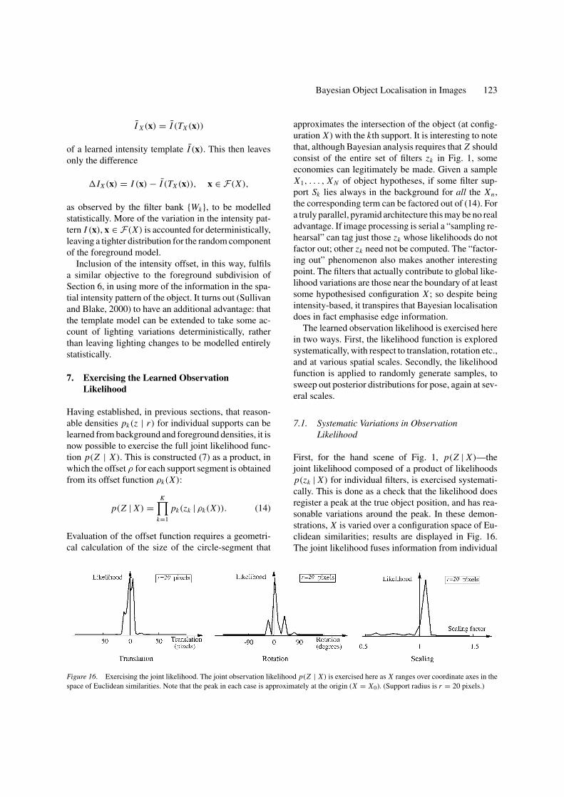
Figure 16. Exercising the joint likelihood. The joint observation likelihood p(Z | X) is exercised here as X ranges over coordinate axes in thespace of Euclidean similarities. Note that the peak in each case is approximately at the origin (X = X0). (Support radius is r = 20 pixels.)

approximates the intersection of the object (at config-uration X ) with the kth support. It is interesting to notethat, although Bayesian analysis requires that Z shouldconsist of the entire set of filters zk in Fig. 1, someeconomies can legitimately be made. Given a sampleX1, . . . , X N of object hypotheses, if some filter sup-port Sk lies always in the background for all the Xn ,the corresponding term can be factored out of (14). Fora truly parallel, pyramid architecture this may be no realadvantage. If image processing is serial a “sampling re-hearsal” can tag just those zk whose likelihoods do notfactor out; other zk need not be computed. The “factor-ing out” phenomenon also makes another interestingpoint. The filters that actually contribute to global like-lihood variations are those near the boundary of at leastsome hypothesised configuration X ; so despite beingintensity-based, it transpires that Bayesian localisationdoes in fact emphasise edge information.

The learned observation likelihood is exercised herein two ways. First, the likelihood function is exploredsystematically, with respect to translation, rotation etc.,and at various spatial scales. Secondly, the likelihoodfunction is applied to randomly generate samples, tosweep out posterior distributions for pose, again at sev-eral scales.

7.1. Systematic Variations in ObservationLikelihood

First, for the hand scene of Fig. 1, p(Z | X)—thejoint likelihood composed of a product of likelihoodsp(zk | X) for individual filters, is exercised systemati-cally. This is done as a check that the likelihood doesregister a peak at the true object position, and has rea-sonable variations around the peak. In these demon-strations, X is varied over a configuration space of Eu-clidean similarities; results are displayed in Fig. 16.The joint likelihood fuses information from individual

124 Sullivan et al.

Figure 17. Joint likelihood at various scales. The observation likelihood p(Z | X) shown for translation, at various scales. Again, modes areapproximately unbiased, and the width of the likelihood peak increases with r .

supports effectively, with a maximal value, as expected,near the true solution X0. Figure 17 demonstrates theeffect of changing the filter scale r . As expected, thelikelihood function is more broadly tuned at coarserscales, appearing to have a width of about 2r , or lessdue to hyperacuity effects as in Fig. 5. As a final check,it is interesting to consider the likelihood ratio for twoconfigurations, one correctly positioned over the tar-get, and one way out over background as in Fig. 1.In such cases, treating pixels as independent typicallyproduces ridiculously large likelihood ratios. Even us-ing Gaussian masks (r = 20), which we know are notindependent, gives a likelihood ratio in this case of1 : 1055—still very large. However, this falls consider-ably with ∇2G masks, as expected given the indepen-dence of their output over foreground and background,to a more plausible 1 : 104.

To summarise, the learned observation likelihood for∇2G masks has been exercised here, systematically,and found to have reasonable properties. The next taskis to use it to compute approximations to the posteriorp(X | Z), by means of the factored sampling schemeof Section 2.4.

7.2. Sampling from the Posterior

To locate a hand against a cluttered background, byBayesian localisation let us assume first that its orien-tation is known but that the prior p(X) for translation isbroad (has high variance). Samples from the posterior,at several scales, are shown in Fig. 18. For a given scale,the broad prior is focused down to a narrow posteriordistribution which, as earlier in Fig. 17, is narrower atfiner scales. It is not clear from Fig. 18 that coarsescales actually have a useful role—the finest scale,after all, gives the most precise information. How-ever, if the sampling process is “pressed” harder, by

expanding the prior without increasing the size N ofthe particle-set, the fine scale breaks down, as Fig. 19shows, while at the two coarser scales, sampling fromthe posterior continues to operate correctly. That sug-gests a role for coarser scales in guiding or constrain-ing finer ones, if only a Bayesian sampling mecha-nism can be found to do it, and that is the subject ofSection 8.

8. Layered Sampling

In Section 7.2, the problem of “overloading” wasdemonstrated, that occurs when image observations aremade at a fine spatial scale. It results from the obser-vation likelihood f (X) having a support that is narrowcompared with the support of the prior p0(X). A con-tinuation algorithm is used to reduce computationalcomplexity by introducing a sequence of likelihoodsfn whose supports are intermediate between those ofp0(X) and f (X), and which reduce progressively insize. One form of this idea is “annealed importancesampling” (Neal, 2000), in which f (X) is replacedby f (X)β , 0 < β < 1 in order to broaden likelihoodfunction. It is known to reduce the number of particlesneeded for estimation (to a given accuracy) by impor-tance sampling, from N to log N .

Layered sampling is an alternative form of contin-uation principle in which the intermediate likelihoodsare obtained by making image measurements at a vari-ety of spatial scales. Filter responses at several scalesr = r1, r2, . . . are used in coarse-to-fine sequence. Sobackground distributions

pB(z | ρ, r), 0 ≤ ρ ≤ 1, r = r1, r2, . . .

need to be learned at each scale, and similarly for fore-ground distributions.


Figure 18. Random samples from the posterior. Factored sampling from the posterior density p(X | Z), in which the prior p(X) is a broaddistribution of Euclidean similarities (planar rigid motion plus size-scaling). At each scale r , the posterior mean E[X | Zr ] (white contour) isclose to the true configuration X0 and the variance of the distribution p(X | Zr ) decreases with r , as expected. Particle set size is N = 80 perlayer. (For clarity, only particles from the posterior accounting for at least 1% of likelihood over sample-set are shown.)

8.1. Importance Reweighting

Layered sampling uses what we term “importancereweighting, in which the particles representing someprior distribution p0(X) are replicated and re-weighted.Particles are replicated to a degree that is propor-tional to the value of some weighting function g(X),as in Fig. 20. Following the re-distribution, likelihoodweights are adjusted to compensate, so that the particle-set continues to represent the same underlying prior p0.The re-weighting operation is denoted by a ∼ operatorwith a weighting function. An example of its use

follows:

p0 −→N

© ∼ g−→N

© × f−→ © ∼−→N

©.

This is factored sampling (9) with an extra, interme-diate, reweighting stage. In terms of particle-sets, thereweighting operation ∼ g is defined as follows{(

s(i), πi), i = 1, . . . , N

}→ {(

s(i( j)), 1/g(s(i( j))

)), j = 1, . . . , N

}where each i( j) is sampled with replacement from i =1, . . . , N with probability proportional to πi g(s(i)).

126 Sullivan et al.

Figure 19. A broader prior “overloads” factored sampling. Now the demonstration of Fig. 18 is repeated, but with a prior 1.5 times as broad,causing sampling at the finest scale to break down (observe the large bias in the mean configurations at scale r = 10, 20 pixels. (Again, N = 80.)

Figure 20. Importance reweighting. A uniform prior p0(X), repre-sented as a particle-set (top), is resampled via an importance functiong to give a new, re-weighted particle-set representation of p0. (Theillustration here is for a one-dimensional distribution, though prac-tically X is multidimensional.)

A useful property of the resampling operation ∼ gis that it is an asymptotic identity: as N → ∞, the dif-ference between the distributions of the two randomvariables generated by

p0 −→N

© ∼−→1

© and by p0 −→N

© ∼g−→N

© ∼−→1

©

converges weakly to 0.Resampling with the ∼ g operation does not, on its

own, deal with the problem of a narrow likelihood func-tion. Although it does concentrate sampling to a nar-rower region of configuration space, the gaps betweenparticles are as great as ever (Fig. 21). Gaps can be


Figure 21. Resampling followed by convolution. This simplifiedexample illustrates that importance reweighting on its own cannotrepopulate the sparsely sampled support of the likelihood f . Re-population can however be achieved by adding a random increment,corresponding to convolving the prior p0 with p1, the density of therandom step.

filled, however, by adding a further random variablewith density p1, to each particle. This has the effect ofdiffusing apart identical copies of particles generatedin the resampling step. Of course, the combined oper-ation is no longer an asymptotic identity—particles atthe output of

p0 −→N

© ∼g−→N

© ∗p1−→ © ∼−→1

©

are distributed asymptotically according to the densityp0 ∗ p1.

8.2. The Layered Sampling Algorithm

Layered sampling is applicable when importance re-sampling functions f1, . . . , fM are available, in whichfM = f is the true likelihood, and each fm−1 is a coarseapproximation to fm . In addition, the prior p0 must bedecomposable as a series of convolutions

p0 = p′0 ∗ p′

1 . . . ∗ p′M−1 (15)

and this corresponds to expressing X a priori as a sumof random variables. Functional forms for the densi-ties p′

m need not necessarily be known, provided onlythat a random sample generator can be constructed foreach. For example, in processing motion sequences us-ing the Condensation algorithm (Isard and Blake,1996), p′

0 could be represented as a set of particlesfrom the previous time t −1, and pd = p′

1 . . .∗ p′M−1 is

some decomposition of a normal distribution pd(X (t) |X (t − 1)) for the likely displacement over one time-

step, into normally distributed components. With thisdecomposition of the prior, the sampling process (9)on page 6 can be replaced by a sequence of layers:

p′0 −→

N©

∼ f1−→N

© ∗p′1−→ ©

· · · (16)

∼ fM−1−→N

© ∗p′M−1−→ ©

× fM−→ © ∼−→N

©.

Each layer includes an importance resampling step,with the observation likelihood fi at the i th scale asthe resampling function, until the M th and final layer,at which the fine-scale fM acts multiplicatively on like-lihood weights, in the usual way.

The asymptotic correctness of layered sampling canbe demonstrated by manipulating the sampling dia-gram. Using the asymptotic identity property of ∼, (16)can be rewritten, deleting resampling links, to give

p′0 −→

N©

∗p′1−→ ©

· · ·∗p′

M−1−→ ©× fM−→ © ∼−→

N©.

and now the p′m convolutions can be composed to give

p′0 ∗ p′

1 ∗ . . . ∗ p′M−1 −→

N© × fM−→ © ∼−→

N©.

which, from (15), and since fM = f , reduces to theoriginal factored sampling process (9).

8.3. Variance Reduction

A remaining problem is how to choose the likelihoodfunctions and the decomposition of pd in such a wayas to minimise the variance of the particle set gener-ated in the final layer. These are complex problems in

128 Sullivan et al.

general, but some progress can be made by setting outthe following special case.

1. The prior p′0 is a rectangular distribution, with a

support of volume a0 in configuration space.2. Each likelihood function fm is idealised as a rect-

angular (uniform) distribution with a support ofvolume am .

3. The support of each fm is a subset of the support offm−1.

4. Each p′m is chosen in such a way that N particles are

effectively uniformly distributed over the supportof fm , as depicted in Fig. 21. This can be done bymatching the support of p′

m−1 to the support of fm .5. Variance minimisation is not well-posed for rect-

angular distribution fm , since their support isbounded. Instead, we minimise the “failure rate”—the probability that the particle set in some layeris empty.

Under these assumptions it can be shown (see ap-pendix) that the failure rate is minimised by choosing

am−1 = λam (17)

so that successive support volumes are in some fixedratio λ.

Three further useful results (derivations omitted) canbe obtained using analysis of estimator variance forimportance sampling (Neal, 2000; Liu and Chen, 1995;Geweke, 1989).

• Using just a single layer (i.e. without layered sam-pling), the number N of particles required to achievea given failure rate is

N ∝ a0/aM (18)

• With layered sampling, the failure rate is minimisedby having approximately

M = log2(a0/aM) (19)

layers. This means that λ = 1/2 is the optimal ratioof support volumes.

• With the optimal number M of layers, the total num-ber of particles required falls to

N M ∝ log2(a0/aM), (20)

a logarithmic speed-up compared with (18).

9. Results

Layered sampling is applied here to the problem ofmulti-scale localisation. In all cases, a hexagonal tes-selation of filters was used with separations of 6σ (Sec-tions 9.1, 9.2), or 3σ (Sections 9.3, 9.4). [Recall thatthe support of the filters are truncated at r = 3σ ; filtersizes are specified as r -values in experiments below.] Aconstant number N of particles was used in each layer;demonstrations with motion in Section 9.4 were donewith just a single layer, though clearly these also wouldbe expected to benefit from multiple layers.

9.1. Sampling Across Scales

In the Bayesian localisation application, the fm fromthe layered sampling algorithm correspond to obser-vation likelihoods from the coarsest scale m = 1 tothe finest m = M . Operation of the algorithm is illus-trated here, in Fig. 22, for the hand-finding problemthat caused the overloading of single-scale samplingearlier, in Section 7.2. The normally distributed priorp0 is split, as a sum of normal variables, into 3 factors

p0 = p′0 ∗ p′

1 ∗ p′2,

each factor to be used before scales r1, r2, r3 in thecoarse-to-fine hierarchy of observations. Scales arechosen to decrease geometrically, as implied by thefixed ratio rule (17) above. (This implication holds onthe assumption that observation likelihood functionsscale linearly with filter radius r , and demonstrationstend to support this, as in Fig. 17). The i th scale gen-erates an observation likelihood function fi , wherefi (X) = p(Zi | X). Note that the formal likelihoodderives from observations only at the finest scale. Ob-servations at other scales are cast by layered samplingin an “advisory” role, their scope limited to importancesampling for the next finer scale. This avoids any needfor any formal assumption of statistical independenceacross scales which may be hard to justify.

9.2. Occlusion

One of the attractions of intensity-based matching isits robustness to disturbances in the image data, and asevere form of disturbance is presented by occlusion.Where occlusion is anticipated, this is addressed inthe Bayesian localisation framework simply by treating


Figure 22. Layered sampling across spatial scales: the demonstration of Fig. 19 is repeated, but now with layered sampling, from coarse to finescale. Note that the overload evident at finest scale in Fig. 19, is rectified here, with a similar computational load (N = 80 particles per layer).

130 Sullivan et al.

Figure 23. Layered sampling with occlusion: a demonstration like the one in Fig. 22 but now with the object suffering unpredicted occlusion.Note that, at the coarsest scale, shape information is sufficiently distorted by occlusion, that object orientation is quite ambiguous in the posterior.Finer scales resolve the ambiguity.


Figure 24. Pose variation: the prior is approximately uniformly distributed (on the white rectangle) over translations, with normal distributionsover pose and zoom. The first and last layers of the posterior from layered sampling with r = 40, 20, 10 pixels are shown, for each of threeposes of a face. (Means displayed in white; N = 250 particles per layer, of which the 15 with highest likelihood are displayed.)

132 Sullivan et al.

the occluder as part of the background, and evaluatingthe appropriate observation-likelihood functions there.More challenging is occlusion that is not anticipated,as in Fig. 23. The figure illustrates the power of theBayesian sampling approach to deal with ambiguity.At coarse scale, the part-occluded and blurred repre-sentation of shape leaves object-orientation quite am-biguous, though translation is somewhat constrained.Finer scales contain fragments of curve at sufficientresolution to register quite precisely with part of theobject outline. Hence the rotational ambiguity is re-solved. Even though the posterior at the finest scale hasvery small variance, nonetheless, the facility to repre-sent ambiguity in the intermediate processes is whathas allowed multi-scale information to be propagatedeffectively.

9.3. Pose Variation

Bayesian localisation is capable of handling a configu-ration spaceX that incorporates varying 3D pose, as thedemonstration of Fig. 24 shows. The foreground distri-butions in this demonstration were learned using fore-ground subdivision as discussed in Section 6, with sub-regions of a diameter equal to that of the filter support.In fact, in the coarsest layer, there is space within theface contour for only one subregion, but 7 subregions atr = 20 and 33 at r = 10. Note the “rogue” face hypoth-esis appearing on the curtain at the left, which receivesa significant weight in layer 1, at the coarsest scale (ablurry hallucination), but does not survive at fine scale.

Figure 25. Deformable motion. A deformable contour model with 8 free parameters is used to track a walking person. The image sequencecontains over 150 image frames. (We used a single layer with r = 15 pixels and N = 1500 samples.)

A further demonstration of face-tracking, free-running at about 1 frame/sec, is given at

http://www.robots.ox.ac.uk/∼vdg/movies/

bayes-face.mpg.

In this case there are two layers with r = 40, 20 andN = 600 particles per layer, and a foreground intensitymodel is used, as in (Sullivan and Blake, 2000).

9.4. Motion Tracking

Motion tracking demonstrations in this section servetwo purposes. First they test the Bayesian localisationalgorithm over many separate video frames. Secondthey underline the importance of Bayesian techniquesfor sequential inference. The prior for object config-uration in each frame is predicted from the posteriorfor the previous frame, via a learned dynamical model(Blake et al., 1995; Baumberg and Hogg, 1995). Theiterated process of prediction and Bayesian localisationforms a particle filter (Gordon et al., 1993; Kitagawa,1996; Isard adn Blake, 1996). A person walking acrossa room is tracked (Fig. 25) in the manner of Baumbergand Hogg’s tracking demonstration (1995), but withoutbackground subtraction. See also the movie version at

http://www.robots.ox.ac.uk/∼vdg/movies/

bayes-walker.mpg.


Instead, distracting background clutter is dealt withby the learned foreground/background models embod-ied in the observation likelihood. Consequently, themethod not limited to backgrounds that are stationary,or moving in some easily predictable fashion.

A note should be added here on computation time.The task (on-line, excluding learning) here consistsprincipally of image processing to obtain the zk , andof computation of likelihood (14), of which the offsetfunction pn(zk | ρk(X)) is main burden. The image pro-cessing can be done using pyramid filter banks (Burt,1983) that are available in hardware. The offset func-tion (at scale r = 40) can be computed for approxi-mately N = 500 particles per time-step, at frame-rate.Bayesian localisation at video frame-rate is thereforequite feasible, in principle.

10. Conclusions

The original elements of Bayesian localisation are:the development of filter-based likelihood functionsfor matching with particular attention to statistical in-dependence; learning of foreground and backgrounddistributions, and distributions for “mixed” receptivefields; probabilistic multi-scale analysis by means of“layered sampling.”

The approach has been tested on a variety of fore-grounds and backgrounds. It is capable of planar objectlocalisation, even with unpredicted occlusion, and ver-satile enough to work with 3D pose changes, and withimage sequences of moving objects, including non-rigid ones. A number of issues are raised: the choiceof partition for the prior in layered sampling; the useof spatio-temporal filters and associated independencearguments; temporal updating of the foreground distri-bution. These remain for future investigation.

Appendix

A. Layered Sampling and Bounded Variance

The result from section 8 about arranging the scales ofsuccessive likelihood functions in fixed ratio is derivedhere. Making the assumptions 1–5 from Section 8.3,the density of particles on entering the mth layer in(16) is N/am−1, assumed uniformly distributed in con-figuration space. Then the proportion of these particles

which lies within the support of fm has mean

λm = am

am−1

and is binomially distributed. The probability P(Fm)

of “failure” at the mth layer is therefore

P(Fm) = (1 − λm)N

and the event F = F1 ∪ . . .∪ FM of failure at any layerhas probability

P(F) = 1 −M∏

i=1

(1 − (1 − λm)N ).

Now minimising P(F) under the constraints that µi ≥0 and the constraint (imposed using a Lagrange multi-plier) that the product

M∏i=1

λi = aM

a0

is a constant, gives a unique solution

λ1 = λ2 = · · · = λM ,

so that the ratios am/am−1 are all equal, as required.

Acknowledgments

We are grateful for the support of the Royal Soci-ety of London (AB), EPSRC (AB,JS,MI) and the EU(JM). We have enjoyed and benefited from discussionswith D. Mumford, S. Mallat, G. Hinton, B. Buxton, A.Zisserman and P. Torr.

Notes

1. Previously (Sullivan et al., 1999) we have referred to the new ap-proach as “Bayesian Correlation,” but have since been persuadedthat this is a somewhat misleading term.

2. The problem of how to obtain the prior p0 is a much debatedissue for Bayesian inference in general which is entirely outsidethe scope of this paper. We simply adopt the common line ofdeveloping a methodology in which the role of the prior is at anyrate explicit.

3. Note that “slicing” is purely an analytical tool to illustrate theway observation likelihoods exist implicitly within a probabilisticmodel for filter response. Slicing does not actually form part ofany algorithm proposed here.

134 Sullivan et al.

4. We refrain from the commonly used term “Laplace” distributionhere, to avoid the potential confusion with the Laplacian operatorin ∇2G.

5. Of course, the filter has theoretically unbounded support, but wetake the point at which filter amplitude falls to around 10% of itsmaximum value.

References

Bartels, R., Beatty, J., and Barsky, B. 1987. An Introduction to Splinesfor use in Computer Graphics and Geometric Modeling. MorganKaufmann: San Mateo, CA.

Bascle, B. and Deriche, R. 1995. Region tracking through imagesequences. In Proc. 5th Int. Conf. on Computer Vision, Boston,pp. 302–307.

Baumberg, A. and Hogg, D. 1995. Generating spatiotemporal modelsfrom examples. In Proc. British Machine Vision Conf., Vol. 2,pp. 413–422.

Belhumeur, P. and Kriegman, D. 1998. What is the set of images of anobject under all possible illumination conditions. Int. J. ComputerVision, 28(3):245–260.

Bell, A. and Sejnowski, T. 1997. Edges are the independent compo-nents of natural scenes. In Advances in Neural Information Pro-cessing Systems, MIT Press: Cambridge, MA, Vol. 9, pp. 831–837.

Beymer, D. and Poggio, T. 1995. Face recognition from one exampleview. In Proc. 5th Int. Conf. on Computer Vision, Boston, USA,pp. 500–507.

Black, M. and Yacoob, Y. 1995. Tracking and recognizing rigid andnon-rigid facial motions using local parametric models of imagemotion. In Proc. 5th Int. Conf. on Computer Vision, Boston, USA,pp. 374–381.

Blake, A. and Isard, M. 1998. Active Contours. Springer: New York.Blake, A., Isard, M., and Reynard, D. 1995. Learning to track

the visual motion of contours. J. Artificial Intelligence, 78:101–134.

Bookstein, F. 1989. Principal warps: Thin-plate splines and the de-composition of deformations. IEEE Trans. on Pattern Analysisand Machine Intelligence, 11(6):567–585.

Burt, P. 1983. Fast algorithms for estimating local image proper-ties. Computer Vision, Graphics and Image Processing, 21:368–382.

Cootes, T., Taylor, C., Cooper, D., and Graham, J. 1995. Activeshape models—their training and application. Computer Visionand Image Understanding, 61(1):38–59.

Field, D. 1987. Relations between the statistics of natural images andthe response properties of cortical cells. J. Optical Soc. of AmericaA., 4:2379–2394.

Gelfand, A. and Smith, A. 1990. Sampling-based approaches to com-puting marginal densities. J. Am. Statistical Assoc., 85(410):398–409.

Geman, D. and Jedynak, B. 1996. An active testing model for track-ing roads in satellite images. IEEE Trans. Pattern Analysis andMachine Intell., 18(1):1–14.

Geman, S. and Geman, D. 1984. Stochastic relaxation, Gibbs distri-butions, and the Bayesian restoration of images. IEEE Trans. onPattern Analysis and Machine Intelligence, 6(6):721–741.

Geweke, J. 1989. Bayesian inference in econometric models usingMonte Carlo integration. Econometrica, 57:1317–1339.

Gordon, N., Salmond, D., and Smith, A. 1993. Novel approach tononlinear/non-Gaussian Bayesian state estimation. IEE Proc. F,140(2):107–113.

Grenander, U. 1976–1981. Lectures in Pattern Theory I, II and III.Springer: New York.

Grenander, U., Chow, Y., and Keenan, D. 1991. HANDS. A Pat-tern Theoretical Study of Biological Shapes. Springer-Verlag:New York.

Grenander, U. and Miller, M. 1994. Representations of knowledge incomplex systems (with discussion). J. Roy. Stat. Soc. B., 56:549–603.

Hager, G. and Toyama, K. 1996. Xvision: Combining image warpingand geometric constraints for fast tracking. In Proc. 4th EuropeanConf. Computer Vision, pp. 507–517.

Isard, M. and Blake, A. 1996. Visual tracking by stochastic propaga-tion of conditional density. In Proc. 4th European Conf. ComputerVision, pp. 343–356, Cambridge: England.

Isard, M. and Blake, A. 1998. Condensation—Conditional densitypropagation for visual tracking. Int. J. Computer Vision, 28(1):5–28.

Kitagawa, G. 1996. Monte Carlo filter and smoother for non-Gaussian nonlinear state space models. Journal of Computationaland Graphical Statistics, 5(1):1–25.

Liu, J. and Chen, R. 1995. Blind deconvolution via sequential impu-tations. J. Am. Stat. Soc, 90(430):567–576.

Mallat, S. 1989. A theory for multiresolution signal decomposition:The wavelet representation. IEEE Trans. on Pattern Analysis andMachine Intelligence, 11:674–693.

Matthies, L., Kanade, T., and Szeliski, R. 1989. Kalman filter-basedalgorithms for estimating depth from image sequences. Int. J.Computer Vision, 3:209–236.

Mumford, D. 1996. Pattern theory: A unifying perspective. In Per-ception as Bayesian Inference, D. Knill, and W. Richard (Eds.),pp. 25–62. Cambridge University Press: Cambridge.

Neal, R. 2000. Annealed importance sampling. Statistics and Com-puting, in press.

Olshausen, B. and Field, D. 1996. Emergence of simple-cell recep-tive field properties by learning a sparse code for natural images.Nature, 381:607–609.

Perona, P. 1992. Steerable-scalable kernels for edge detection andjunction analysis. J. Image and Vision Computing, 10(10):663–672.

Ripley, B. 1992. Classification and clustering in spatial and imagedata. In Procs. 15 Jahrestagung von Gesellschaft fur Klassifika-tion. H. Goebl and M. Schader (Eds.), Springer-Verlag: New York.

Scharstein, D. and Szeliski, R. 1998. Stereo matching with nonlineardiffusion. Int. J. Computer Vision, 28(2):155–174.

Shirai, Y. and Nishimoto, Y. 1985. A stereo method using disparityhistograms and multi-resolution channels. In Proc. 3rd Int. Symp.on Robotics Research, pp. 27–32.

Storvik, G. 1994. A Bayesian approach to dynamic contoursthrough stochastic sampling and simulated annealing. IEEETrans. on Pattern Analysis and Machine Intelligence, 16(10):976–986.

Sullivan, J. and Blake, A. 2000. Satistical foreground modelling forobject localisation. In Proc. European Conf. Computer Vision,vol. 2, pp. 307–323.

Sullivan, J., Blake, A., Isard, M., and MacCormick, J. 1999. Objectlocalisation by Bayesian correlation. In Proc. 7th Int. Conf. onComputer Vision, pp. 1068–1075.


Szeliski, R. 1990. Bayesian modelling of uncertainty in low-levelvision. Int. J. Computer Vision, 5(3):271–301.

Vetter, T. and Poggio, T. 1996. Image synthesis from a single exampleimage. In Proc. 4th European Conf. Computer Vision, Cambridge:England, pp. 652–659.

Viola, P. and Wells, W. 1993. Alignment by maximisation of mu-tual information. In Proc. 5th Int. Conf. on Computer Vision,pp. 16–23.

Witkin, A., Terzopoulos, D., and Kass, M. 1987. Signal matchingthrough scale space. Int. J. Computer Vision, 1(2):133–144.

Zhu, S. and Mumford, D. 1997. GRADE: Gibbs reaction and dif-fusion equation. IEEE Trans. on Pattern Analysis and MachineIntelligence, 19(11):1236–1250.

Zhu, S., Wu, Y., and Mumford, D. 1998. Filters, random fields andmaximum entropy (FRAME). Int. J. Computer Vision, 27(2):107–126.

Documents

Bayesian Object Localisation in Images - Temple …latecki/Courses/RobotFall07/PapersFall07...Bayesian Object Localisation in Images ... that has undergone certain distortions