Embed Size (px)
Citation preview

Bayesian Networks in Educational Testing
Ji rı Vomlel
Institute of Information Theory and AutomationAcademy of Science of the Czech Republic
Prague
This presentation is available at:http://www.utia.cas.cz/vomlel/

Contents:• What is a Bayesian network?
• Student model and evidence models.
• A case study: Students perfoming computations with fractions.
• Variables in the student model.
• Construction of the student model.
• Evidence models.
• Construction of an adaptive test.
• Construction of a fixed test.
• Results of experiments.

Bayesian networkX1 X2P (X1) P (X2)
P (X3 | X1)
P (X4 | X2)
P (X6 | X3, X4)
P (X9 | X6)
P (X8 | X7, X6)
P (X5 | X1)
P (X7 | X5)
X5
X7
X3
X8
X6
X9
X4
P (X1, . . . , X9) =
= P (X9|X8, . . . , X1) · P (X8|X7, . . . , X1) · . . . · P (X2|X1) · P (X1)
= P (X9|X6) · P (X8|X7, X6) · P (X7|X5) · P (X6|X4, X3)
·P (X5|X1) · P (X4|X2) · P (X3|X1) · P (X2) · P (X1)

Student and evidence models(R. Almond and R. Mislevy, 1999)
S4
X2
S1 S3
S4
S2S3
X3
S2
X1
S3
S5
S1
S5

Sudents solving problems with fractions• A group of university students from Aalborg University prepared
paper tests that were given to students at Brønderslev HighSchool.
• Four elementary skills, four operational skills, and abilities toapply operational skills to complex tasks were tested.
• 149 students solved the test.
• The tests were analyzed in detail so that it was possible for mostof students to decide whether they have or have not the testedskills.
• Several different models were learned using the PC algorithm
• Models were compared on how well they predict skills using theleave-one-out method.

Examples of tasks - operations withfractions
T1:(
34· 5
6
)− 1
8= 15
24− 1
8= 5
8− 1
8= 4
8= 1
2
T2: 16
+ 112
= 212
+ 112
= 312
= 14
T3: 14· 11
2= 1
4· 3
2= 3
8
T4:(
12· 1
2
)·(
13
+ 13
)= 1
4· 2
3= 2
12= 1
6.

Elementary and operational skillsCP Comparison (common nu-
merator or denominator)
12
> 13, 2
3> 1
3
AD Addition (comm. denom.) 17
+ 27
= 1+27
= 37
SB Subtract. (comm. denom.) 25− 1
5= 2−1
5= 1
5
MT Multiplication 12· 3
5= 3
10
CD Common denominator`
12, 2
3
´=
`36, 4
6
´CL Cancelling out 4
6= 2·2
2·3 = 23
CIM Conv. to mixed numbers 72
= 3·2+12
= 3 12
CMI Conv. to improp. fractions 3 12
= 3·2+12
= 72

Misconceptions
Label Description Occurrence
MAD ab + c
d = a+cb+d 14.8%
MSB ab −
cd = a−c
b−d 9.4%
MMT1 ab ·
cb = a·c
b 14.1%
MMT2 ab ·
cb = a+c
b·b 8.1%
MMT3 ab ·
cd = a·d
b·c 15.4%
MMT4 ab ·
cd = a·c
b+d 8.1%
MC a bc = a·b
c 4.0%
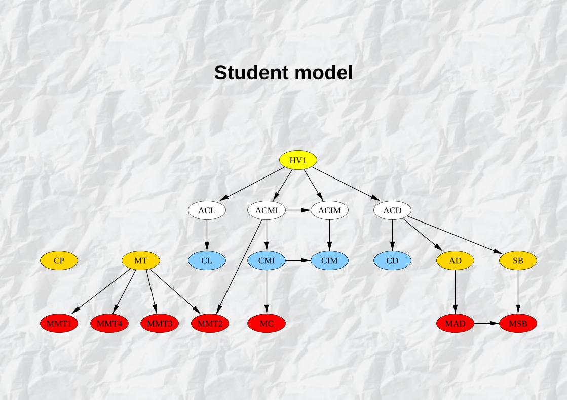
Student model
MMT1
HV1
CP MT
MMT4 MMT2MMT3 MC MAD MSB
SBADCDCIMCMICL
ACL ACMI ACIM ACD

Evidence model for task T1„3
4· 5
6
«− 1
8=
15
24− 1
8=
5
8− 1
8=
4
8=
1
2
T1 ⇔ MT & CL & ACL & SB & ¬MMT3 & ¬MMT4 & ¬MSB
CL
MMT4
MSB
SB
MMT3
ACL MT
T1
X1
P (X1 | T1)

The overal model

See the model in Hugin:http://www.hugin.com

Tested models
(a) two hidden variables with several restrictions on presence or absence of edges,
(b) two hidden variables and only few restrictions,
(c) one hidden variable and few restrictions,
(d) no hidden variable and few restrictions,
(e) no hidden variable and only obvious logical constraints as restrictions,
(f) no hidden variable and independent skills,
(g) Naıve Bayes model with one hidden variable (with two states) being parent ofall skills,
(h) as above, but the hidden variable has three states,

Comparison of different models using tvalues
vs. (b) vs. (c) vs. (d) vs. (e) vs. (f) vs. (g) vs. (h) total
(a) −3.293 −2.650 −2.567 0.308 2.323 −1.318 −2.192 −3
(b) 0.983 0.578 3.579 5.296 1.734 0.759 +3
(c) −0.265 2.612 4.488 1.154 −0.004 +3
(d) 2.839 4.487 1.327 0.091 +3
(e) 3.837 −1.977 −2.739 −4
(f) −4.071 −4.728 −7
(g) −1.641 +2
(h) +3

Fixed Test vs. Adaptive Test
wrong
correct wrong
wrong correct
wrong
wrong
correct
correctwrong wrongcorrectcorrectcorrect
Q5
Q4
Q3
Q2
Q1
Q2
Q1
Q3
Q4
Q5
Q6
Q7
Q8
Q9
Q10
Q6 Q8
Q7
Q8
Q4 Q7 Q10
Q6
Q7
Q9

Entropy as an information criteria
0
0.1
0.2
0.3
0.4
0.5
0.6
0.7
0 0.2 0.4 0.6 0.8 1
-x*log(x)-(1-x)*log(1-x)
Entropy of probability distribution P (S) on skills S is defined as
H (P (S)) = −∑s
P (S = s) · log P (S = s)
“The lower the entropy the more we know about a student.”

X3
X1
X3
X3
X2
X3
X2
X1
X2
X1
X2
X2
X3
X1
X1
Entropy in node n
H(en) = H(P (S | en))
Expected entropy at the end of test t
EH(t) =∑
`∈L(t)
P (e`) ·H(e`)
T ... the set of all possible tests
(e.g. of a given length)
A test t? is optimal iff
t? = arg mint∈T
EH(t) .

A myopically optimal test t is a test where each question X? of t
minimizes the expected value of entropy after the question is
answered:
X? = arg minX∈X
EH(t↓X) ,
i.e. it works as if the test finished after the selected question X?.

X3
X1
X3
X3
X2
X3
X2
X1
X2
X1
X2
X2
X3
X1
P (X2 = 1)
X1
P (X2 = 0)
e list = {{X2 = 0}, {X2 = 1}}
counts[3] = P (X2 = 0) = 0.7
counts[1] = P (X2 = 1) = 0.3
X2 X3 . . .
Myopic construction of a fixed test
e list := [∅];test := [ ];
for i := 1 to |X | do counts[i] := 0;
for position := 1 to test lenght do
new e list := [ ];
for all e ∈ e list do
i := most informative X(e);
counts[i] := counts[i] + P (e);
for all xi ∈ Xi do
append(new e list, {e ∪ {Xi = xi}});e list := new e list;
i? := arg maxi counts[i];
append(test, Xi?);
counts[i?] := 0;
return(test);

Entropy of the probability distributions on the skills
4
5
6
7
8
9
10
11
12
0 2 4 6 8 10 12 14 16 18 20
Entr
opy
on s
kills
Number of answered questions
adaptiveaverage
descendingascending

Skill Prediction Quality
74
76
78
80
82
84
86
88
90
92
0 2 4 6 8 10 12 14 16 18 20
Qua
lity
of s
kill
pred
icti
ons
Number of answered questions
adaptiveaverage
descendingascending

Conclusions
• Empirical evidence shows that educational testing can benefitfrom application of Bayesian networks. Adaptive tests maysubstantially reduce the number of questions that arenecessary to be asked.
• Method for the design of a fixed test provided good results ontested data. It may be regarded as a good cheap alternative tocomputerized adaptive tests when they are not suitable.
• One theoretical problem related to application of Bayesiannetworks to educational testing is efficient inference exploitingdeterministic relations in the model. This problem is a topic ofour current research.