Embed Size (px)
Citation preview

Bayesian Learning for NonlinearSystem Identification
Page 1 of 1
20/12/2013file:///D:/Downloads/Imperial_College_London_crest.svg
Wei Pan
Department of BioengineeringImperial College London
This thesis is submitted for the degree ofDoctor of Philosophy
March 2017


I would like to dedicate this thesis to my loving parents.


Declaration of Originality
I hereby declare that this thesis was entirely my own work and that any additionalsources of information have been duly cited.
I hereby declare that any internet sources, published or unpublished works fromwhich I have quoted or drawn reference have been reference fully in the text andin the contents list. I understand that failure to do this will result in failure of thisproject due to Plagiarism.
I understand I may be called for a viva and if so must attend. I acknowledge thatwas my responsibility to check whether I am required to attend and that I will beavailable during the viva period.
Wei PanMarch 2017


Copyright Declaration
The copyright of this thesis rests with the author and is made available under a Cre-ative Commons Attribution Non-Commercial No Derivatives licence. Researchersare free to copy, distribute or transmit the thesis on the condition that they attribute it,that they do not use it for commercial purposes and that they do not alter, transformor build upon it. For any reuse or redistribution, researchers must make clear toothers the licence terms of this work.
Wei PanMarch 2017


Acknowledgements
First, I want to deeply thank my supervisor, Dr. Guy-Bart Stan, for his encour-agement and guidance and support for my research all these years, as well as forproviding a unique free and open environment that allows me pursue my owninterest. I appreciate all his contributions of ideas, time, funding to make my Ph.D.study an open eye journey.
I would like to thank Dr. Ye Yuan, my long term collaborator. I can always findspark when we discuss in London, Cambridge, Luxembourg and Wuhan. Thanks,Ye, for everything. I have been so fortunate to collaborate and benefit from manygreat minds: Prof. Jorge Gonçalves, Prof. Mauricio Barahona, Dr. Aivar Sootla, Dr.Wei Dai, Prof. Lennart Ljung, Prof. Henrik Sandberg, Dr. Neil Dalchau, Dr. AndrewPhilips and Prof. Yike Guo. Every tiny detail on meetings, discussions, presentationsand paper writing suddenly came out of my mind. I apologise not to include all theaspects I learn from you simply because there are too many. Thank you all.
I am indebted to my undergraduate supervisor, Prof. Huijun Gao, for the invalu-able advice and support he has been giving me all these years. I would also to thankProf. Zidong Wang, my role model through years. I felt lucky to reunion with youin London.
Outside the lab, I like to thank all the friends I have met here in London, for theirfriendship and the many wonderful moments they have shared with me, and fortheir kind help and support during various stages of my stay here.
I also would like to thank two companies I’ve worked for during my Ph.D.study: Active Securities and Cardwell Investment Technologies, who showed methe possibilities of my work in financial industry.
Last but not least, I want to acknowledge and thank the support of my research.This research was generously supported by Microsoft Research, Dorothy-HodgkinPostgraduate Award, Department of Bioengineering.


Abstract
Prediction and control of behaviour and abnormalities in any complex dynamicalsystems, and in particular those encountered in biology, physics, engineering requirethe development of multivariate mechanistic and predictive models that integratelarge datasets from different sources. Although, a large amount of data are beingcollected on a daily basis, very few methods allow the automatic creation from thesedata of nonlinear dynamical models for understanding and (re-)design/control,and an inordinate amount of time is still being spent on the manual aggregation ofinformation and development of models that explains these data.
In particular, this thesis considers sparse modelling and estimation for a selectionof nonlinear dynamical systems classes. There are two key features of modern timeseries data, i.e., high dimensionality and large scale. The dimensionality, or thecomplexity, grew with the sample size, and “ultra-high” refers to the case wherethe dimensionality increased at a non-polynomial rate. Scale, or the size, refers tothe dimension of the system, i.e., the number of state variables. This work aims todesign a framework and associated algorithms for the identification of a variety ofnonlinear dynamical systems encountered in practice from high-dimensional andlarge-scale time series data.
In the first part of the thesis, we introduce the type of time series data and theclass of nonlinear dynamical system considered in this thesis. Both a selection oftime-invariant and time-varying nonlinear dynamical systems are covered. Fortime-invariant system, the classic nonlinear system identification problem fromsingle dataset is addressed in the beginning. Then we move to a more practicaland significant yet complicated scenario where heterogeneous datasets are usedsimultaneously. Such datasets typically contain (a) data from several replicatesof an experiment performed on a biological system of interest and/or (b) datameasured from a biochemical system subjected to different experimental conditions,for example, changes/perturbations in biological inductions, temperature, geneknock-out, gene over-expression, etc. For time-varying systems, the regime-switchsystem identification problem is considered, i.e., the problem of identifying both

xii
the switching points and the nonlinear model structure within each regime. Thenthe abrupt change point detection problem is considered. Using these, the classictrending filtering and fault diagnosis problems are revisited. All the identificationproblems are formulated as various ℓ0 type optimisation problems. In the end, wediscuss some technical issues on data processing arising from practical applications.
In the second part of the thesis, a repository of algorithms are derived respectivelyfor each identification problem formulated in the first part. These algorithms are notdistinct and can be formulated in a unified way using Bayesian Learning with struc-tural sparse prior. Furthermore, we suggest a series of iterative reweighted convexrelaxation schemes for connecting these algorithms to popular algorithms includingLasso, Group-Lasso, Generalised-Lasso, Fused-Lasso and Graphical-Lasso. In thispart, we go beyond from simple nonlinear model class to more general class; fromdata likelihood in Gaussian distribution to the more general exponential family. Theestimation of the stochastic term also discussed including ARMA and ARCH. Manyoptimisation framework, such as (stochastic) gradient descent, Newton method,Quasi-Newton method, alternating direction method of multiplier can be seamlesslyintegrated into our formulation as either centralised or distributed optimisationstrategy to address high dimensionality and large scale problems. These algorithmslargely enrich not only the family of time series modelling algorithms but also sparsesignal recovery/modelling/estimation algorithms in various communities.
In the third part of the thesis, several time series modelling applications fromsystems biology, complex networks and power systems are given to illustrate theeffectiveness of our modelling framework.
Last but not least, two future research directions based on the output of thisthesis are pointed out, both related to “brains”. The first is focusing on theory andalgorithm about modelling/identification/learning on deep neural networks. Thesecond is focusing applications in neuroscience: understanding the neural basis ofdecision making using mathematical modelling from big data.

Abbreviations and SymbolsAbbreviations and Symbols
Roman Symbols
ADMM Alternative Direction Method of Multiplier
AIC Akaike Information Criterion
ARCH Autoregressive Conditional Heteroskedasticity
ARMA Autoregressive Moving Average
ARMAX Autoregressive Moving Average with External Input
ARX Autoregressive with External Input
BIC Bayesian Information Criterion
CCCP Convex-Concave Procedure or Concave-Convex Procedure
DC Difference of Convex Functions
DNN Deep Neural Networks
DL Deep Learning
GRN Genetic of Regulatory textbfNetworks
KKT Karush-Kuhn-Tucker
LS Least Square
MAP Maximum a Posteriori
MIMO Multiple Input Multiple Output
ML Maximum Likelihood

xivxviii Abbreviations and Symbols
MLE Maximum Likelihood Estimate
MM Majorisation-Minimisation
NARX Nonlinear Autoregressive with External Input
NN Neural Networks
NP Non-deterministic Polynomial-time
PLS Penalised Least Square
RIP Restricted Isometry Property
SBL Sparse Bayesian Learning
SISO Single Input Single Output
SYSID System Identfication
w.r.t. with repect to
Subscripts
FFF 2 RM⇥N a matrix in RM⇥N
FFFi, j 2 R element in the ith row and jth column of a matrix
FFFi,: the ith row of a matrix
FFF:, j the jth column of a matrix
aaa 2 RN⇥1 a column vector in RN
ai the ith element of a vector
IIIL a identity matrix of size L⇥L, we simply use III when the dimension is obviousfrom context
kbbbkp ,kbbbk`p`p norm of a vector bbb 2 RN , that is kbbbk`p
, pq
ÂNi=1 bbb p
i
kbbbk0 ,kbbbk`0`0-quasinorm is the number of non-zero elements in a vector
diag [g1, . . . ,gN ] a diagonal matrix with principal diagonal elements being g1, . . . ,gN
E(aaa) the expectation of the stochastic variable aaa

xv
Abbreviations and Symbols xix
µ proportional to
, defined as
blkdiag[FFF[1], . . . ,FFF[C]] a block diagonal matrix with principal diagonal blocks beingFFF[1], . . . ,FFF[C] in turn
Tr(FFF) the trace of a matrixFFF
FFF ⌫ 000 the matrix FFF is positive semidefinite


Table of contents
List of figures xxiii
List of tables xxv
1 Introduction 11.1 System Identification . . . . . . . . . . . . . . . . . . . . . . . . . . . . 2
1.1.1 The Omni-present Model . . . . . . . . . . . . . . . . . . . . . 21.1.2 System Identification: Data Driven Modelling . . . . . . . . . 31.1.3 The State-of-the-Art Identification Setup . . . . . . . . . . . . 3
1.2 Convex Optimisation . . . . . . . . . . . . . . . . . . . . . . . . . . . . 51.2.1 Convex Relaxation . . . . . . . . . . . . . . . . . . . . . . . . . 51.2.2 Convex Concave Procedure . . . . . . . . . . . . . . . . . . . . 5
1.3 Sparse Signal Recovery . . . . . . . . . . . . . . . . . . . . . . . . . . . 61.4 Machine Learning . . . . . . . . . . . . . . . . . . . . . . . . . . . . . . 8
1.4.1 Why Choose Marginal Likelihood . . . . . . . . . . . . . . . . 101.4.2 Why Choose Sparse Bayesian Learning . . . . . . . . . . . . . 11
1.5 The Big Picture and Contributions . . . . . . . . . . . . . . . . . . . . 141.5.1 A Story on Healthcare . . . . . . . . . . . . . . . . . . . . . . . 141.5.2 Strategy . . . . . . . . . . . . . . . . . . . . . . . . . . . . . . . 151.5.3 Contributions and Outlines . . . . . . . . . . . . . . . . . . . . 17
I Dynamical Systems 21
2 Nonlinear Dynamical Systems 232.1 Introduction . . . . . . . . . . . . . . . . . . . . . . . . . . . . . . . . . 242.2 Linear Time-Invariant Systems . . . . . . . . . . . . . . . . . . . . . . 25
2.2.1 Impulse Response and Transfer Function . . . . . . . . . . . . 252.2.2 Linear Models and Sets of Linear Models . . . . . . . . . . . . 27

xviii Table of contents
2.2.3 ARX Model Structure . . . . . . . . . . . . . . . . . . . . . . . 282.2.4 ARMAX Model Structure . . . . . . . . . . . . . . . . . . . . . 292.2.5 Linear Regression Model . . . . . . . . . . . . . . . . . . . . . 30
2.3 Nonlinear Time-Invariant Systems . . . . . . . . . . . . . . . . . . . . 302.3.1 Nonlinear Time-Invariant Systems . . . . . . . . . . . . . . . . 322.3.2 Some Key Assumptions . . . . . . . . . . . . . . . . . . . . . . 332.3.3 Linear Regression Model . . . . . . . . . . . . . . . . . . . . . 362.3.4 Additional Experiment Designs . . . . . . . . . . . . . . . . . 40
2.4 Linear Regression Problem . . . . . . . . . . . . . . . . . . . . . . . . . 442.4.1 Regression Problem Statement . . . . . . . . . . . . . . . . . . 442.4.2 Nonconvex Optimisation Problem . . . . . . . . . . . . . . . . 442.4.3 Convex Relaxation . . . . . . . . . . . . . . . . . . . . . . . . . 45
3 Nonlinear Dynamical System with Heterogeneous Datasets 473.1 Introduction . . . . . . . . . . . . . . . . . . . . . . . . . . . . . . . . . 483.2 Linear Regression Model . . . . . . . . . . . . . . . . . . . . . . . . . . 493.3 Linear Regression Problem . . . . . . . . . . . . . . . . . . . . . . . . . 51
3.3.1 Regression Problem Statement . . . . . . . . . . . . . . . . . . 513.3.2 Nonconvex Optimisation Problem . . . . . . . . . . . . . . . . 523.3.3 Convex Relaxation . . . . . . . . . . . . . . . . . . . . . . . . . 53
4 Time-Varying Dynamical System 554.1 Introduction . . . . . . . . . . . . . . . . . . . . . . . . . . . . . . . . . 564.2 Regime-Switch Dynamical System . . . . . . . . . . . . . . . . . . . . 57
4.2.1 Scalar Linear Regime-Switch Systems . . . . . . . . . . . . . . 574.2.2 Multivariate Regime-Switch Nonlinear Systems . . . . . . . . 58
4.3 Linear Regression Model . . . . . . . . . . . . . . . . . . . . . . . . . . 594.4 Linear Regression Problem . . . . . . . . . . . . . . . . . . . . . . . . . 60
4.4.1 Regression Problem Statement . . . . . . . . . . . . . . . . . . 604.4.2 Nonconvex Optimisation Problem . . . . . . . . . . . . . . . . 614.4.3 Convex Relaxation . . . . . . . . . . . . . . . . . . . . . . . . . 62
4.5 Models with Abrupt Change . . . . . . . . . . . . . . . . . . . . . . . 634.5.1 Trend Filtering . . . . . . . . . . . . . . . . . . . . . . . . . . . 634.5.2 Fault Diagnosis Problem . . . . . . . . . . . . . . . . . . . . . . 65
5 Technical Issues Related to Dynamical System Identification 675.1 Uniquesness of Solutions in Chapter 2 . . . . . . . . . . . . . . . . . . 68

Table of contents xix
5.2 Selection of Candidate Basis Functions . . . . . . . . . . . . . . . . . . 705.3 Dealing with Basis Function Nonlinearity . . . . . . . . . . . . . . . . 725.4 Gaussian Assumption . . . . . . . . . . . . . . . . . . . . . . . . . . . 735.5 Dealing with Measurement Noise . . . . . . . . . . . . . . . . . . . . . 755.6 Estimation of the Derivative . . . . . . . . . . . . . . . . . . . . . . . . 77
II Algorithms 79
6 Algorithms for Likelihood in Gaussian 816.1 Gaussian Likelihood . . . . . . . . . . . . . . . . . . . . . . . . . . . . 836.2 Sparse Prior . . . . . . . . . . . . . . . . . . . . . . . . . . . . . . . . . 846.3 Optimisation Problem Definition . . . . . . . . . . . . . . . . . . . . . 866.4 Optimisation Principle . . . . . . . . . . . . . . . . . . . . . . . . . . . 906.5 Optimisation Algorithm . . . . . . . . . . . . . . . . . . . . . . . . . . 92
6.5.1 Iterative Reweighted ℓ1 Algorithm . . . . . . . . . . . . . . . . 926.5.2 Iterative Reweighted ℓ2 Algorithm . . . . . . . . . . . . . . . . 946.5.3 Inverse Covariance Matrix Estimation . . . . . . . . . . . . . . 956.5.4 Volatility Estimation . . . . . . . . . . . . . . . . . . . . . . . . 97
6.6 Algorithms for Chapter 2 . . . . . . . . . . . . . . . . . . . . . . . . . . 1006.6.1 Sparse Prior for Chapter 2 . . . . . . . . . . . . . . . . . . . . . 1006.6.2 Optimisation Problem Derivation . . . . . . . . . . . . . . . . 1016.6.3 Centralised Optimisation Algorithm . . . . . . . . . . . . . . . 1026.6.4 Distributed Optimisation Algorithm . . . . . . . . . . . . . . . 116
6.7 Algorithms for Chapter 3 . . . . . . . . . . . . . . . . . . . . . . . . . . 1216.7.1 Sparse Prior for Chapter 3 . . . . . . . . . . . . . . . . . . . . . 1226.7.2 Optimisation Algorithm . . . . . . . . . . . . . . . . . . . . . . 123
6.8 Algorithms for Chapter 4 . . . . . . . . . . . . . . . . . . . . . . . . . . 1266.8.1 Sparse Prior for Chapter 4 . . . . . . . . . . . . . . . . . . . . . 1266.8.2 Optimisation Algorithm . . . . . . . . . . . . . . . . . . . . . . 128
7 Algorithms for Likelihood in Exponential Family 1317.1 Likelihood in Exponential Family . . . . . . . . . . . . . . . . . . . . . 1327.2 Sparse Prior . . . . . . . . . . . . . . . . . . . . . . . . . . . . . . . . . 133
7.2.1 Generalised Sparse Prior . . . . . . . . . . . . . . . . . . . . . . 1337.2.2 Group Sparse Prior . . . . . . . . . . . . . . . . . . . . . . . . . 1347.2.3 Fused Sparse Prior . . . . . . . . . . . . . . . . . . . . . . . . . 136
xx Table of contents
7.3 Optimisation Problem Definition . . . . . . . . . . . . . . . . . . . . . 1377.4 Optimisation Algorithm . . . . . . . . . . . . . . . . . . . . . . . . . . 143
7.4.1 Optimisation for unknown parameter β and hyperparameter γ 1437.4.2 Optimisation for the parameter of the exponential family θ . . 1497.4.3 Implementations . . . . . . . . . . . . . . . . . . . . . . . . . . 150
7.5 Optimisation Algorithm with Structural Sparsity . . . . . . . . . . . . 1567.5.1 Algorithm for Group Spare Prior in Section 7.2.2 . . . . . . . . 1567.5.2 Algorithm for Fused Sparse Prior in Section 7.2.3 . . . . . . . 159
8 Algorithms for Online Model Selection 1698.1 Extended Kalman Filter . . . . . . . . . . . . . . . . . . . . . . . . . . 1708.2 Algorithm combining model structure identification and model re-
finement . . . . . . . . . . . . . . . . . . . . . . . . . . . . . . . . . . . 172
9 Algorithms for Fault Diagnosis 1759.1 Fault Diagnosis Problem Formulation . . . . . . . . . . . . . . . . . . 1769.2 Fault Detection and Isolation Algorithm . . . . . . . . . . . . . . . . . 1779.3 Fault Identification Algorithm . . . . . . . . . . . . . . . . . . . . . . . 177
III Applications 181
10 Biochemical Reaction Network Identification 18310.1 Identification from Single Time Series Data . . . . . . . . . . . . . . . 18410.2 Identificaton from Multiple Heterogeneous Time Series Datasets . . . 18910.3 Online Model Selection . . . . . . . . . . . . . . . . . . . . . . . . . . . 191
10.3.1 Background . . . . . . . . . . . . . . . . . . . . . . . . . . . . . 19110.3.2 Questions of interest . . . . . . . . . . . . . . . . . . . . . . . . 19410.3.3 Simulations . . . . . . . . . . . . . . . . . . . . . . . . . . . . . 195
10.4 Identificaton Switched Biochemical Reation Networks . . . . . . . . . 198
11 Complex Network Reconstruction 20111.1 Centralised Identification . . . . . . . . . . . . . . . . . . . . . . . . . 20211.2 Distributed Identification . . . . . . . . . . . . . . . . . . . . . . . . . 206
12 Fault Diagnosis of Power System 21312.1 Introduction . . . . . . . . . . . . . . . . . . . . . . . . . . . . . . . . . 21412.2 Power System Model . . . . . . . . . . . . . . . . . . . . . . . . . . . . 215

Table of contents xxi
12.3 Fault Diagnosis Problem of Nonlinear Power Systems . . . . . . . . . 21812.3.1 Model Transformation . . . . . . . . . . . . . . . . . . . . . . . 21812.3.2 Fault Diagnosis Algorithm . . . . . . . . . . . . . . . . . . . . 220
12.4 Numerical Study . . . . . . . . . . . . . . . . . . . . . . . . . . . . . . 22412.5 Conclusion and Discussion . . . . . . . . . . . . . . . . . . . . . . . . 225
IV Conclusion and Future Direction 229
13 Conclusion 231
14 Future Direction 23514.1 Future Direction I: Bayesian Deep Learning . . . . . . . . . . . . . . . 236
14.1.1 Background on Deep Learning and Deep Neural Networks . 23614.1.2 Structural Sparsity in Deep Neural Network . . . . . . . . . . 23914.1.3 Identifiability of Deep Neural Networks . . . . . . . . . . . . . 24514.1.4 Training Bayesian Deep Neural Network with Structural Sparsity24914.1.5 Implementation on Mobile Device Chips . . . . . . . . . . . . 250
14.2 Future Direction II: Decision Making in Neuroscience . . . . . . . . . 25414.2.1 Cognitive Design Principles for Real-Time Decision Making
using Neural Big Data . . . . . . . . . . . . . . . . . . . . . . . 25414.2.2 Background . . . . . . . . . . . . . . . . . . . . . . . . . . . . . 25514.2.3 Hypothesis and Objectives . . . . . . . . . . . . . . . . . . . . 25814.2.4 Problems and Plan . . . . . . . . . . . . . . . . . . . . . . . . . 259
References 267


List of figures
1.1 The identification work loop (Coutersey of Professor Lennart Ljung). 4
1.2 Schematic illustration of the evolution of dynamical model duirngdisease progression . . . . . . . . . . . . . . . . . . . . . . . . . . . . . 14
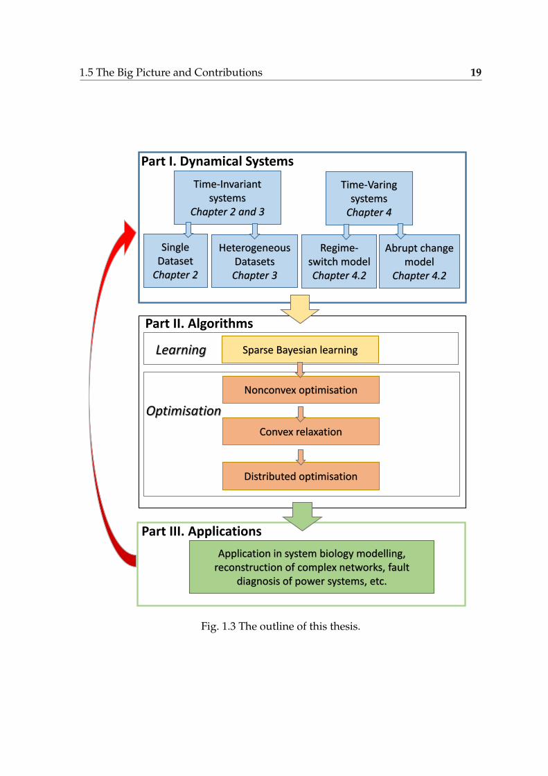
1.3 The outline of this thesis. . . . . . . . . . . . . . . . . . . . . . . . . . . 19
10.1 Root of Normalised Mean Square Error ∥βestimate − βtrue∥2/∥βtrue∥2
averaged over 200 independent experiments for the signal-to-noiseratios 0 dB, 5 dB, 10 dB, 15 dB, 20 dB, and 25 dB. . . . . . . . . . . . . 188
10.2 Computational running time averaged over 200 independent exper-iments for the signal-to-noise ratios 0 dB, 5 dB, 10 dB, 15 dB, 20 dB,and 25 dB. . . . . . . . . . . . . . . . . . . . . . . . . . . . . . . . . . . 188
10.3 Algorithm comparison in terms of RNMSE ∥βestimate − βtrue∥2/∥βtrue∥2
averaged over 50 independent experiments. . . . . . . . . . . . . . . . 192
10.4 Technological platform for in-vivo model selection of synthetic cir-cuits. In this closed loop configuration the computer (upper rightcorner) takes images of the cells in the microfluidic device (lower leftcorner) via a microscope (upper left corner), quantifies the output ofthe network of interest in real time and applies the next sample ofinput(s) via the fluidic pressure actuation system (lower right corner). 193
10.7 Estimation of the time-varying parameters. . . . . . . . . . . . . . . . 200
11.1 Parameter RNMSE and computational running time averaged over200 independent experiments for the signal-to-noise ratios 0 dB, 5 dB,10 dB, 15 dB, 20 dB, and 25 dB. . . . . . . . . . . . . . . . . . . . . . . 205
11.2 Phase diagrams for Algorithm 4. . . . . . . . . . . . . . . . . . . . . . 207
11.3 Average computational running time. . . . . . . . . . . . . . . . . . . 209

xxiv List of figures
12.1 Time-series of yi for all buses. The black dashed lines indicate thethreshold σ∗ in Algorithm 20. The coloured solid lines are the phaseangle measurements for bus i, i = 5, 7, 11, 16, 19. At time instant t =3.02s, |y5|, |y7|, |y11|, |y16| and |y19| are much greater than σ∗ (σ∗ = 10here). . . . . . . . . . . . . . . . . . . . . . . . . . . . . . . . . . . . . . 225
12.2 Time-series of the sparsity of the estimated fault, i.e. ∥wfaulti −wtrue
i ∥0
for bus i = 5, 7, 11, 16, 19. . . . . . . . . . . . . . . . . . . . . . . . . . 22612.3 Identification of transmission lines faults. . . . . . . . . . . . . . . . . 227
14.2 A graphical illustration on the strategy of removing the filters inconvolutional neural networks . . . . . . . . . . . . . . . . . . . . . . 242
14.3 A graphical representation of LSTM memory cells (there are minordifferences in comparison to Graves [70]). . . . . . . . . . . . . . . . . 243
14.4 A graphical illustration on the model reduction technique in controltheory . . . . . . . . . . . . . . . . . . . . . . . . . . . . . . . . . . . . . 244
14.5 A graphical illustration of DropNeuron strategy in regression problem249

List of tables
1.1 The unified work flow for algorithm derivations in Chapters 6, 7 ofPart II . . . . . . . . . . . . . . . . . . . . . . . . . . . . . . . . . . . . 18
14.1 Summary of statistics for Sparse Regression . . . . . . . . . . . . . . . 249


Chapter 1
Introduction

2 Introduction
1.1 System Identification
During the thesis author’s visit to Professor Lennart Ljung’s group at LinköpingUniversity, who is the authority in the field of system identification (SYSID), a seriesof ideas were shared on SYSID. I would like to quote and summarise these ideas inwhat follows.
1.1.1 The Omni-present Model
It is clear to everyone in science and engineering that mathematical models areplaying increasingly important roles. Today, model-based design and optimizationis the dominant engineering paradigm to systematic design and maintenance ofengineering systems. It has proven very successful and is widely used in basicallyall engineering disciplines. Concerning control applications, the aerospace industryis the earliest example on a grand-scale of this paradigm. This industry was veryquick to adopt the theory for model based optimal control that emerged in the1960s, and is spending great efforts and resources on developing models. In theprocess industry, Model Predictive Control (MPC) has during the last 25 yearsbecome the dominant method to optimize production on an intermediate level.MPC uses dynamical models to predict future process behaviour and to optimizethe manipulated variables subject to process constraints.
Increasing demands on performance, efficiency, safety and environmental aspectsare pushing engineering systems to become increasingly complex. Advances in(wireless) communications systems and micro-electronics are key enablers for thisrapid development; allowing systems to be efficiently inter-connected in networks,reducing costs and size and paving the way for new sensors and actuators.
Model-based techniques are also gaining importance outside engineering appli-cations. Let us just mention systems biology and health care. In the latter case it isexpected that personalised health systems will become more and more important inthe future.
Common to the examples given above are the requirements of integrating sensingactuation, communication and computation abilities of the engineering systems, inmany cases in distributed architectures. It is also clear that these systems shouldbe able to operate in a reliable way in an uncertain and temporally and spatiallychanging environment. In many applications, cognitive abilities and abilities toadapt will be important. With systems being decentralized and typically containingmany actuators, sensors, states and non-linearities, but with limited access to sensor

1.1 System Identification 3
information, model building that delivers models of sufficient fidelity becomes verychallenging.
1.1.2 System Identification: Data Driven Modelling
Construction of models requires access to observed data. It could be that the modelis developed entirely from information in signals from the system (“black boxmodels”), or it could be that physical/engineering insights are combined with suchinformation (“grey box models”). In any case, verification (validation) of a modelmust be done in the light of measured data. Theories and methodologies for suchmodel construction have been developed in many different research communities(to some extent independently). System Identification is the term used in the ControlCommunity for the area of constructing mathematical models of dynamical systemsfrom measured input/output signals. Other communities use other terms for oftenvery similar techniques. The term Machine Learning has become very common inrecent years.
System identification has a history of more than 50 years since the term wascoined by Lotfi Zadeh, [227]. It is a mature research field with numerous publications,text books, conference series, and software packages. It is often used as an examplein the control field of an area with good interaction between theory and industrialpractice. The backbone of the theory relies upon statistical grounds, with maximumlikelihood and asymptotic analysis (in the number of observed data). The goal of theSYSID field is to find a model of the plant in question as well as of its disturbanceand also to find a characterisation of the uncertainty bound of the description.
1.1.3 The State-of-the-Art Identification Setup
To approach a SYSID problem, a number of questions need to be answered, like
• what model type should be used?
• how should the parameters in the model be adjusted?
• what inputs should be applied to obtain a good model?
• how do we assess the quality of the model?
• how do we gain confidence in an estimated model?

4 Introduction
M IM(θ)
XD
V
OK?No, try new M Yes!
No, try newX
Fig. 1.1 The identification work loop (Coutersey of Professor Lennart Ljung).
There is a very extensive literature on the subject, with many text books [117, 175,227]. The SYSID problem is usually formulated mathematically by introducing thefollowing notations
• X : The experimental conditions under which the data is generated
• D: The data
• M: The Model Structure and its parameters β
• I: The identification method by which a parameter value β in the modelstructureM(β) is determined based on the data D
• V : The validation process that scrutinises the identified model.
The identification of a model is typically an iterative process that involves passingthrough the non-invalidation test step (“the model is not falsified (so far)”), andalso involving various revisions of the modelling choices. that passes through thevalidation test (“is not falsified”), involving revisions of the necessary choices. Forseveral of the steps in this loop helpful support tools have been developed. Itis not quite possible or desirable to fully automate the choices, since subjectiveperspectives, related to the intended use of the model are very important.

1.2 Convex Optimisation 5
1.2 Convex Optimisation
1.2.1 Convex Relaxation
Convex optimisation is a special class of mathematical optimisation problems for whichthere are efficient polynomial time algorithms that are guaranteed to converge to aglobal minimum [28]. Least square, linear programming, semidefinite programming,second order cone programming are all convex optimisation problems. If a problemcan be formulated as a convex problem, it can be reliably and efficiently solved,for instance, using interior point methods. There are free optimisation packages(i.e., solvers) such as SDPT3 [193] and SeDuMi [183] for solving convex programs.Moreover, user-friendly modelling languages such as CVX and YALMIP [119] makethese solvers accessible for a wide range of users.
On the contrary to convex problems, non-convex problems usually have lots oflocal minima where optimisation algorithms are likely to get trapped if not initialisedproperly. Convex relaxation can be used to approximate (in some cases, even exactlysolve for) the global optimum of a non-convex problem in a principled way. In somecases, they can also be used to find bounds on the global optimum or to provide agood point for gradient search.
In this thesis, all the SYSID problems are recast into appropriate optimisationproblems. Unfortunately, these problems are usually non-convex and NP-hard.Nevertheless, resorting to convex relaxations, we obtain efficient solutions. In whatfollows some important convex relaxations, which play a central role in deriving ourmain results, are summarised. It is important to note that this Section is by no meansa comprehensive treatment of the subject. Rather, it aims at giving a basic intuitionbehind each relaxation together with readily usable, relaxed, convex formulationsthat will help the reader understand the development in the proceeding Chapters.
1.2.2 Convex Concave Procedure
The Convex Concave Procedure (CCCP) [226] is a majorisation-minimisation (MM)algorithm [92] that is popularly used to solve DC (difference of convex functions).Its main idea is to yield an iterative scheme for
minx∈C
f(x)
6 Introduction
with C ⊆ Rp where each iteration consists of minimising a so-called majorisationfunction f(x, x(k)) of f(x) at x(k) ∈ C
x(k+1) = argminx∈C
f(x, x(k)
)(1.1)
where f : C×C → R satisfies f(x, x) = f(x) for x ∈ C and f(x) ≤ f(x, z) for x, z ∈ C.Clearly, (1.1) yields a descent algorithm. Construction of a suitable majorisationfunction is a key step for MM algorithm. For difference of convex programmingproblems minx∈C f(x) where
f(x) = u(x)− v(x),
u, v : C → R are convex and differentiable functions with C being a convex set in Rp,there are many ways to construct the majorisation function [92]. The simplest one isthe so-called linear majorisation via “supporting hyperplane” [92], i.e.,
f(x, x(k)
)= u(x)− v
(x(k)
)−∇v
(x(k)
)⊤ (x− x(k)
). (1.2)
For this particular choice of majorisation function, it is also referred to as “sequentialconvex optimisation”.
The convergence of MM algorithm to a stationary point (the point satisfies theKarush-Kuhn-Tucker (KKT) conditions, see e.g., [28]) has been discussed in e.g.,[179].
1.3 Sparse Signal Recovery
In this Section, we present the background results on the problem of sparse signalrecovery [31, 196, 50] that motivates the approach pursued in this thesis.
The Sparse signal recovery problem can be stated as: given some linear mea-surements y = Xβ of a discrete signal β ∈ RN where X ∈ RM×N , M ≪ N , findthe sparsest signal β∗ consistent with the measurements. In terms of the ℓ0 quasi-norm (i.e. ∥ · ∥ℓ0 or ∥ · ∥0 satisfies all of the norm axioms except homogeneity since∥cx∥0 = ∥β∥0 for all non-zero scalars c), this problem can be recast into the followingoptimisation form:
min ∥β∥ℓ0 subject to: y = Xβ. (1.3)

1.3 Sparse Signal Recovery 7
When the measurements are contaminated with some noise, the optimisation prob-lem can be formulated as a regularised linear regression form:
minβ∥y−Xβ∥2
2 + λ ∥β∥ℓ0. (1.4)
where λ is a tradeoff parameter or the regularisation parameter. It is well knownthat the optimisation problems above are at least generically non-deterministicpolynomial-time (NP)-complete. Two fundamental questions in sparse signal re-covery are: (i) the uniqueness of the sparse solution, (ii) the existence of efficientalgorithms for finding such a solution. In the past few years it has been shown thatif the matrix A satisfies the so-called restricted isometry property (RIP), the solutionis unique and can be recovered efficiently by several algorithms. These algorithmsfall into two main categories: greedy algorithms (e.g. orthogonal matching pursuit[195, 197, 129, 44]) and ℓ1-based convex relaxation (also known as basis pursuit[31, 196, 50]).
As shown in [31], the RIP condition is a sufficient condition for exact recon-struction based on ℓ1-minimisation. It was shown in [31, 44, 30] that both convexℓ1-minimisations and greedy algorithms lead to exact reconstruction of S-sparse sig-nals if the matrix X satisfies the RIP condition. The ℓ1 relaxation of the optimisationproblem in (1.4) is
minβ∥y−Xβ∥2
2 + λ ∥β∥ℓ1 (1.5)
The idea behind this relaxation is the fact that the ℓ1 norm is the convex envelope ortightest convex relaxation of the ℓ0 norm, and thus, in a sense, minimizing the formeryields the best convex relaxation to the (non-convex) problem of minimising thelatter. Moreover, as shown in [31, 196, 50], this relaxation is stable and robust to noise.That is, even when only noisy linear measurements are available, if RIP holds forX, which is true with high probability for random matrices, recovery of the correctsupport of the original signal and approximating the true value within a factor ofthe noise is always possible. This formulation arises naturally in many engineeringapplications such as magnetic resonance imaging, radar signal processing and imageprocessing. Moreover, existence of efficient algorithms to solve this problem led tothe compressive sensing framework which enabled speeding up signal acquisitionconsiderably since the original sparse signal can be reconstructed using relativelyfew measurements.

8 Introduction
One major drawback of the RIP condition is that it can be very difficult to check(combinatorial search). Another related and easier-to-check property is the coherenceproperty.
Definition 1 (mutual coherence [52]) For any matrix X = [X:,1, . . . , X:,N ] ∈ RM×N ,the coherence of a matrix X is defined as
µ(X) = max1≤j,k≤N,j =k
|⟨X:,j, X:,k⟩|∥X:,j∥2∥X:,k∥2
. (1.6)
As shown in [51], for a column normalised matrix X, i.e., ∥X:,i∥2 = 1, ℓ1-minimisationsolutions are equivalent to ℓ0-minimisation solutions if, for a solution, y = Xβ, thefollowing condition is satisfied:
∥β∥0 <12
(1 + 1
µ(X)
)(1.7)
It was also shown that RIP guarantees incoherence of X, i.e. µ(X) ≈ 0, [31]. Thismeans one is guaranteed that ℓ1-minimisation solutions are equivalent to the truesolution only when X is near orthogonal, i.e. when the columns of X are stronglyuncorrelated.
Revisit the background of SYSID problems in Section 1.1 for a moment. As wewill show in Part II of the thesis, SYSID problems can be formulated as ℓ0 normregularised optimisation problems such as (1.4) and its variations. The dictionarymatrix X is constructed directly from time series data or certain transformation ofthe data. Quite often, correlation between the columns of Φ is typically high (closeto 1) and the RIP condition and low coherence condition are hardly guaranteed. Inpractice, ℓ1 relaxation based algorithms do not yield the optimal solution.
1.4 Machine Learning
The Machine Learning community is huge. The success of machine learning appli-cations has boosted and been boosting the development of our modern societies.An exhaustive literature review on machine learning is not necessary in this the-sis. Several excellent textbooks will give an overview, technique explanations andapplications of machine learning, e.g., [22, 79, 127], to just name a few.
In this Section we would like to offer an insight into the links that exist betweenmachine learning and the system identification problem that we introduced earlier.

1.4 Machine Learning 9
We do this as inference tools from machine learning since they are superior in certainaspects to the conventional approaches in SYSID. Until very recently, there has beenlittle contact between these concepts and system identification.
Recent research has shown that model selection problems can be successfullydealt with using a different approach to SYSID that leads to an interesting crossfertilization with the machine learning field [151]. Rather than postulating finite-dimensional hypothesis spaces, e.g. using ARX, ARMAX or Laguerre models, thenew paradigm formulates the problem as function estimation possibly in an infinite-dimensional space. In the context of linear system identification, the elements ofsuch space are all possible impulse responses. The intrinsical ill-posedness of theproblem is circumvented using regularization methods that also admit a Bayesianinterpretation [158]. In particular, the impulse response is modelled as a zero-meanGaussian process. In this way, prior information is introduced in the identificationprocess just assigning a covariance, named also kernel in the machine learningliterature [166]. In view of the increasing importance of these kernel methods alsoin the general SYSID scenario, some of the key mathematical tools and conceptof these learning techniques should be made accessible to the control community,e.g. reproducing kernel Hilbert spaces [8, 156], kernel methods and regularisationnetworks [58, 148, 202] and the connection with the theory of Gaussian processes[81, 158]. It is also worth noting that a straight application of these techniques in thecontrol field is doomed to fail unless some key features of the system identificationproblem are taken into account. First, as already recalled, the relationship betweenthe unknown function and the measurements is not direct, as typically assumed inthe machine learning setting, but instead indirect, through the convolution with thesystem input. Furthermore, in system identification it is essential that the estimationprocess be informed on the stability of the impulse response. In this regard, a recentmajor advance has been the introduction of new kernels which include informationon impulse response exponential stability [36, 151]. These kernels depend on somehyperparameters which can be estimated from data e.g. using marginal likelihoodmaximization. This procedure is interpretable as the counterpart of model orderselection in the classical PEM paradigm but, as it will be shown, it turns out to bemuch more robust, appearing to be the real reason of success of these new procedures.Other research directions recently developed have been the justification of the newkernels in terms of Maximum Entropy arguments [152], the analysis of these newapproaches in a classical deterministic framework leading to the derivation of the

10 Introduction
optimal kernel [36], as well as the extension of these new techniques to the estimationof optimal predictors [150].
Next we would like to introduce two topics or concepts in machine learningwhich will be mainly applied in this thesis.
1.4.1 Why Choose Marginal Likelihood
The benefit of marginal likelihood can be quoted and summarised from [208] andProfessor Michael Jordan’s lectures on “Bayesian Modelling and Inference” at UCBerkeley. If one were to plot the “classical” likelihood with respect to the “complexity”of the model, one would find that as the complexity of the model increased, sowould the likelihood. In this setting, the likelihood is obtained after estimatingthe parameters using some statistical methods (e.g. maximum likelihood), andthen plotting the value of P(y|β). However, the problem of using this methodof comparison is that more “complex” models will always do better than simplermodels. Because more complex models have more parameters, whatever can bedone in a simple model can be done in a complex model, and thus, a more complexmodel will lead to a beeter fit. The downside is that this leads to overfitting, whichis particularly damaging in the setting of prediction. In frequentist statistics, manymethods have been developed to penalise the likelihood with respect to increasingcomplexity of the model. However, these methods are typically only justified afterproposing the idea and then performing a series of analyses to show that it hasdesirable properties, rather than being will-motivated from the start.
In the Bayesian framework, marginal likelihoods have a natural built-in penaltyfor more complex modes. At a certain point, the marginal likelihood will begin todecrease with increasing complexity, and hence, does not directly suffer from theoverfitting problem that occurs when considering only likelihoods. The intuitionfor why the marginal likelihood will begin to decrease with increasing complexityis that as the complexity of the model increases, the prior will be spread out morethinly across both the “good” models and the “bad” models. Because the marginallikelihood is the likelihood integrated with respect to the prior, spreading the prioracross too many models will place too little prior mass on the good models, and as aresult, cause the marginal likelihood to decrease.

1.4 Machine Learning 11
Another way to look at it is as follows. Suppose y is the data, β are the parametersandM is the models
P(β|y,M) = P(y|β,M)P(β|M)P(y|M) . (1.8)
Solving for the marginal likelihood P(y|M) in (1.8), we obtain
P(y|M) = P(y|β,M)P(β|M)P(β|y,M) . (1.9)
Taking the log of (1.9) results in
log P(y|M) = log P(y|β,M)︸ ︷︷ ︸log likelihood
+ log P(β|M)− log P(β|y,M)︸ ︷︷ ︸penalty
(1.10)
This is true for any choice of β, and in particular, the maximum likelihoodestimate of β. The log P(y|β,M) term in (1.10) is the log likelihood, and only in-creases with increasing model complexity. On the other hand, the log P(β|M) −log P(β|y,M) term can be viewed as a “penalty” that penalises against complexmodels. The overall sign of this penalty is negative because P(β|y,M), the poste-rior, is generally larger than P(β|M), the prior, assuming that given the data, theposterior “sharpens” up with respect to the prior. Hence, the penalty term balancesout the increase in likelihood as the model complexity increases.
1.4.2 Why Choose Sparse Bayesian Learning
Referencing several excellent Ph.D. thesis relevant to SBL [215, 10, 231], the ad-vantage of choosing SBL for proposing solutions to the SYSID problem can besummarised as follows
1. It is known that SBL algorithms have achieved top performance in manypractical problems, or even solved some bottlenecks which other sparse signalrecovery algorithms cannot solve [232, 233]. Besides, it is interesting to seethat SBL has connections to Lasso-type algorithms, therefore, one can modifyexisting Lasso-type algorithms or design new Lasso-type algorithms to exploita special, application-specific structure for better performance.
2. Its recovery performance is robust to the characteristics of the matrix X, whileother algorithms are not. For example, it has been shown that when columns

12 Introduction
of X are highly coherent, SBL still maintains good performance, while otheralgorithms such as Lasso or other algorithms based on convex relaxationshave seriously degraded performance [216]. Experiments also showed thatwhen X is a non-random matrix or a sparse matrix, SBL algorithms maintainexcellent performance. This advantage is very attractive to feature selectionin bioinformatics, source localisation, and other applications, since in theseapplication X is not a random matrix and its column are highly correlated.Such situation is very often encountered in SYSID problems, or general timeseries modelling problems, where X is constructed from time series data.
3. SBL has a number of desired advantages over many popular algorithms interms of local and global convergence. It can be shown that SBL provides asparser solution than Lasso-type algorithms [212]. In particular, in noiselesssituations and under certain conditions, the global minimum of the SBL costfunction is unique and corresponds to the true sparsest solution, while theglobal minimum of the cost function of Lassotype algorithms is not necessarilythe true sparsest solution [213, 218]. Besides, it can be shown [214] that incertain settings, Lasso-type algorithms and ℓp (p < 1) minimisation algorithmsalways fail, while SBL succeed, regardless of X and the sparsity of β. Theseadvantages imply that SBL is a better choice in spare signal recovery andSYSID problems.
4. SBL provides scale-invariant solutions, while Lasso-type algorithms cannot[214]. Let βSBL be the optimal solution provided by SBL with the sensing matrixX. With a diagonal matrix D, i.e., X → XD, the optimal solution providedby SBL becomes DβSBL. In contrast, for Lasso-type algorithms, there is nosuch linear relationship between the solutions. For example, the solution tothe problem min ∥y−Xβ∥2
2 + λ∥β∥1 has no such linear relationship with thesolution to the rescaled problem min ∥y −XDβ∥2
2 + λ∥β∥ℓ1 . This warns thatrescaling X may be problematic in SYSID problems when time series data arenormalised and the re-weighting procedure is used for each iteration of theiterative algorithms.
Admittedly, SBL is not perfect. The main drawback is that SBL generally involveslarge computational loads. Some strategies have been used to speed up SBL. Forexample, using the marginalized likelihood method [192], several fast algorithmshave been derived [95, 9]. Using the connection between SBL and Lasso-typealgorithms [212, 235], one can obtain optimal SBL solutions by iteratively performing

1.4 Machine Learning 13
Lasso-type algorithms several times. Since Lasso-type algorithms become moreefficient year by year, using this iteration strategy also greatly benefits SBL. However,SBL is still slower than some efficient algorithms, such as greedy algorithms ormessage passing algorithms. Thus, new strategies are required to speed up SBL, andmore efficient SBL algorithms are needed.
Another drawback of SBL is that the estimation of noise variance is not reliable.Learning rules for the noise variance in most SBL algorithms are not effective innoisy environments. Thus, most SBL algorithms [213, 218, 95, 217] use some fixedsub-optimal values, or require users or other algorithms to provide the value, insteadof learning it. Recently, an effective empirical strategy to enhance these learningrules has been proposed [235, 234], which helps SBL achieve satisfactory solutions.However, this strategy does not completely solve this problem. More effectivemethods and theoretical guidance are called for.

14 Introduction
1.5 The Big Picture and Contributions
The main content of thesis is based on this thesis author’s publications with co-authors. All of these publications are peer reviewed and the thesis author is the firstauthor of all of them [138, 141, 143, 142, 136, 137, 139, 140].
1.5.1 A Story on Healthcare
The treatment of some disease relies on the development and evaluation of multi-variate predictive models, to give “the right treatment to the right patient at the righttime” by integrating large dataset from different sources. One important questionfrom the patient is “what is my individual prognosis?” This question cannot alwaysbe easily answered by doctors. As an aid to diagnostics and treatment design amodel can be developed to identify different patterns of progression based on sensordata from wearable devices for example.
Although the elapsed time between disease onset and the collection of datasamples may be unknown, the samples are normally classified with staging phases(e.g. prognosis stages) that characterise the clinical or pathological status of diseaseprogression. For each patient, a personalised and tailored dynamical model needs tobe developed to explain the observations at each stage, see Figure 1.2.
Fig. 1.2 Schematic illustration of the evolution of dynamical model duirng diseaseprogression

1.5 The Big Picture and Contributions 15
For each individual patient k, k = 1, . . . , K, the dynamic model can be specifiedby differential/difference equations
δxk(t) =
fk1(xk(t), pk1), if t ∈ [tk1, tk2), Stage 1fk2(xk(t), pk2), if t ∈ [tk2, tk3), Stage 2...
......
fks(xk(t), pks), if t ∈ [tk,start, tk,end], Stage s
. (1.11)
δ denotes the differentiation operator for continuous-time systems, or the shiftoperator for discrete-time system. xk is the quantity of interested observed for thek-th individual. fks describes the dynamics of xk and pks are the correspondingparameters of fks. It should be noted that fks may be nonlinear. tks denotes thestarting time of stage s, start = 1, . . . , s (s may be unknown). Then the modelidentification problem of interest can be summarised as follows:
Problem 1 For each patient k, given the observed the heterogeneous sample-based datasetxk(t), we are interested in identifying the onset time tk,start of stage s; the form of fks and theassociated parameters pks at each stage s.
1.5.2 Strategy
At time instant t, the system in (1.11) for the patient k, can be expressed as a linearcombination of several dictionary functions by letting yk(t) ≜ δxk(t) as the output,
yk(t) =N∑
n=1Xkn(t)βkn(t), (1.12)
Xkn encodes the type of functions f(xk(t), pk) that are used to describe the system,βkn encodes the unknown parameter pk. For nonlinear systems, more details onsuch expansion can be found in [138, 136, 143, 139, 140].
Problem formulation
If there is no switch (s = 1 in (1.11) and βkn(t) = βkn, ∀t) and only one patient’s datais collected, the model identification problem can be formulated as the followingregularised regression problem (see [138, 136, 139])
minβ
12
T∑t=1∥y(t)−
N∑n=1
Xn(t)βn∥22 + λ
N∑n=1∥βn∥ℓ0 . (1.13)

16 Introduction
In particular when the data is contaminated by measurement noise, the problemis discussed in [137]. If all the K patients’ data are taken into account, the modelidentification problem can be formulated as (see [140])
minβ
12
K∑k=1
T∑t=1∥yk(t)−
N∑n=1
Xkn(t)βkn∥22 + λ
N∑n=1
∥∥∥∥∥√∑K
k=1 w2kn
∥∥∥∥∥ℓ0
. (1.14)
If there are switches (s > 1 in (1.11)) and only one patient’s data is collected, themodel identification problem can be formulated as (see [143]),
minβ
12
T∑t=1∥y(t)−
N∑n=1
Xkn(t)βkn(t)∥22
λ1
T∑t=1
N∑n=1∥βkn(t)∥ℓ0 + λ2
T −1∑t=1
+N∑
n=1∥βkn(t + 1)− βkn(t)∥ℓ0 .
(1.15)
Algorithm Development
The regularised regression problems in Eqs. (1.13)-(1.15) are NP-hard. To be able tooffer some time-efficient solution to this optimisation problem, one typically consid-ers empirical relaxations to this optimisation problem, e.g. replacing ℓ0 with ℓ1 min-imisation, which is known to give the tightest convex relaxation to ℓ0 minimisationproblems. This gives rise to the well-known Lasso type algorithms [188, 189, 62, 190].However, such empirical relaxations sometimes yield poor performance mainly dueto the high coherence of the dictionary matrix [52]. The variational Bayesian frame-work often yields better performance by integrating the marginal likelihood maximi-sation and usage of hyperparameter to control the sparsity. One of the drawbacksof the Bayesian framework is the associated computational cost, which is higherin comparison with currently existing state-of-art algorithms. In [136, 140, 137],distributed convex optimisation algorithms are proposed to identify large-scalenonlinear state-space systems from high-dimensional time series data, i.e., largeK, T, N in Eqs. (1.13)-(1.15). This algorithm can exploit multiple computation unitsin parallel which makes big time series data modelling possible.
Real-time Monitoring
Another important problem is to monitor the status of the patient and give earlydiagnostic and warning signals before before his health state starts to deteriorate.This can be formulated as a problem of detecting the change point of βkn(t) when

1.5 The Big Picture and Contributions 17
βkn(t + 1)− βkn(t) = 0 . A similar mathematical problem for large-scale nonlinearpower systems has been investigated in [141, 142], i.e. the problem of fault diagnosison transmission lines. The strategy can be potentially applied to diseases withdifferent patterns of progression.
Pharmacokinetics
Last but not least, prediction of human pharmacokinetics, dose and drug interactionsis also of importance. If some measured quantity of interest is treated as output andthe dosage of certain drugs is treated as input, a personalised transfer function frominput to output should be calibrated for each patient. The modelling techniques in[138, 136, 140, 137] can be potentially used to this effect.
1.5.3 Contributions and Outlines
The central hypothesis of the thesis is that a suite of learning and optimisationtechniques based on exhibiting structures and sparseness can and will enable moreaccurate reliable solutions to larger and richer time series modelling across a widevariety of domains. In particular, this thesis focuses on addressing both statisticaland computational aspects of learning from high-dimensional large-scale structuredtime series data in the following three different aspects:
Statistical modelling of nonlinear dynamical systems from time series data: InPart I of the thesis, we propose a series of sparse statistical modelling formulationsby exploiting the structural information in both the time series data and dynamicalsystems. In Chapter 2, we deal with the identification of time-invariant nonlineardynamical system from a single dataset [138, 136, 139]. In Chapter 3, we consider theidentification of time-invariant nonlinear dynamical system, but from heterogeneousdatasets [140]. In Chapter 3, we focus on time-varying dynamical systems. In thefirst part of Chapter 3, we investigate regime-switch systems modelling from “static”time series data [143]; in the second part, we investigate the identification of “abruptchange” models from “streaming” time series data and in particular the trendfiltering and fault diagnosis problems [141, 142]. At the end of Part I, we discusssome technical issues related to dynamical systems identification, model structureselections, and data preprocessing in practice.

18 Introduction
Learning and optimisation framework for large-scale and high-dimensional timeseries data: In Part II of the thesis, a scalable, general algorithm framework basedon machine learning and convex optimisation is proposed for the inference ofmodels presented in Part I. A schematic of the work flow for algorithm derivationsin Chapters 6, 7 of Part II can be summarised in Table 1.1.
1. Specify the likelihood of the data;
2. Specify the structural sparse prior controlled by structured hyperparametersfor various penalties in the original ℓ0 problem;
3. Formulate the nonconvex optimisation problem joint in both parameter to beestimated and hyperparameters using a marginal likelihood maximisationframework;
4. Apply the convex concave procedure to convexify the nonconvex optimisa-tion problem;
5. Derive the iterative re-weighed ℓ1 or ℓ2 type algorithm (the first iterationusually start with the empirical Lasso/Ridge regression type algorithms);
6. (Optionally) Formulate the distributed version of the algorithm for “big data”analysis purposes.
Table 1.1 The unified work flow for algorithm derivations in Chapters 6, 7 of Part II
Applications In Part III, we apply the proposed methods to a broad class of prob-lems in systems biology, physics and engineering [137].
A schematic of the structure of this thesis is shown in Figure 1.3. It coversthe nonlinear systems class in this thesis and two technical foundations for thealgorithms developed in this thesis is illustrated, i.e., machine learning and convexoptimisation. In particular, we emphasise the importance of closing the loop (thered arrow on the left of Figure 1.3) from Part III to Part I. Modelling time series datarequires deep understanding and insight into the underlying dynamical systems ofspecific application domains.
1.5 The Big Picture and Contributions 19
Time-Invariant systems
Chapter 2 and 3
Time-Varingsystems
Chapter 4
Single Dataset
Chapter 2
Heterogeneous DatasetsChapter 3
Regime-switch modelChapter 4.2
Abrupt change model
Chapter 4.2
Part I. Dynamical Systems
Sparse Bayesian learning
Nonconvex optimisation
Convex relaxation
Distributed optimisation
Part II. Algorithms
Application in system biology modelling, reconstruction of complex networks, fault
diagnosis of power systems, etc.
Learning
Optimisation
Part III. Applications
Fig. 1.3 The outline of this thesis.


Part I
Dynamical Systems


Chapter 2
Nonlinear Dynamical Systems

24 Nonlinear Dynamical Systems
2.1 Introduction
Identification of nonlinear dynamical systems from noisy time-series data is rel-evant to many different fields such as systems/synthetic biology, econometrics,finance, chemical engineering, social networks, etc. Yet, the development of generalreconstruction techniques remains challenging, especially due to the difficulty ofadequately identifying nonlinear systems [117]. Nonlinear dynamical system re-construction aims at recovering the set of nonlinear equations associated with thesystem from noisy time-series observations. The importance of nonlinear structureidentification and its associated difficulties have been widely recognised [118, 173].
Since, typically, nonlinear functional forms can be expanded as sums of termsbelonging to a family of parameterised functions (see Sec. 5.4, [117]), an usualapproach to identify nonlinear black-box models is to search amongst a set of possi-ble nonlinear terms (e.g., basis functions) for a parsimonious description coherentwith the available data [72]. A few choices for basis functions are provided byclassical functional decomposition methods such as Volterra expansion, Taylor poly-nomial expansion or Fourier series [117, 15]. This is typically used to model systemssuch as those described by Wiener and Volterra series [210, 15], neural networks[128], nonlinear auto-regressive with exogenous inputs (NARX) models [112], andHammerstein-Wiener [12] structures, to name just a few examples.
Graphical models have been proposed to capture the structure of nonlineardynamical networks. In the standard graphical models where each state variablerepresents a node in the graph and is treated as a random variable, the nonlinearrelation among nodes can be characterised by factorising the joint probability dis-tribution according to a certain directed graph [104, 147, 177]. However, standardgraphical models are often not adequate for dealing with times series directly. Thisis mainly due to two aspects inherent to the construction of graphical models. Thefirst aspect pertains to the efficiency of graphical models built using time series data.In this case, the building of graphical models requires the estimation of conditionaldistributions with a large number of random variables [16] (each time series is mod-elled as a finite sequence of random variables), which is typically not efficient. Thesecond aspect pertains to the estimation of the moments of conditional distribution,which is very hard to do with a limited amount of data especially when the systemto reconstruct is nonlinear. In the case of linear dynamical systems, the first two mo-ments can sometimes be estimated from limited amount of data [11, 123]. However,
2.2 Linear Time-Invariant Systems 25
higher moments typically need to be estimated if the system under consideration isnonlinear.
In this Chapter, we will start with an introduction to linear time-invariant systemsin Section 2.2; then we will extend this introduction to nonlinear time-invariantsystems in Section 2.3; in Section 2.4, we will give the regression problem formulationfor the nonlinear SYSID problem from single experiment. The regression problem isfurther formulated as a ℓ0 type optimisation problem in Section 2.4.2 and a tentativeempirical ℓ1 relaxation is proposed in Section 2.4.3. At the end of the Chapter,we discuss the uniqueness of the solution and the selection of the basis functions.The latter discussion also applies to other Chapters throughout this thesis. Thealgorithms for this Chapter will be provided in Section 6.6 of Chapter 6.
2.2 Linear Time-Invariant Systems
2.2.1 Impulse Response and Transfer Function
Impulse Response
As in [117], we first introduce some preliminary for impulse response and transferfunction. Consider a system with a scalar input signal u(t) and a scalar output signaly(t). The system is said to be time invariant if its response to a certain input signaldoes not depend on absolute time. It is said to be linear if its output responses to alinear combination of inputs is the same linear combination of the output responsesof the individual inputss. Furthermore, it is said to be causal if the output at a certaintime depends on the input up to that time only.
It is well known that a linear, time-invariant, causal system can be described byits impulse response (or weighting functions) g(τ) as follows:
y(t) =∫ ∞
τ=0g(τ)u(t− τ)dτ (2.1)
Knowing {g(τ)}∞τ=0 and knowing u(s) for s ≤ t, we can consequently compute the
corresponding output y(s), s ≤ t for any inputs. The impulse response is thus acomplete characterisation of the system.
In practice, 1). inputs and outputs are observed in discrete time due to the typicaldata-acquisition mode; 2). disturbance is ubiquitous due to measurement noiseand/or uncontrollable inputs. We thus assume y(t) to be observed at the samplinginstants tk = kT , k = 1, 2, . . .: y(kT ) =
∫∞τ=0 g(τ)u(kT − τ)dτ . The interval T will be

26 Nonlinear Dynamical Systems
called the sampling interval. It is, of course, also possible to consider the situationwhere the sampling instants are not equally spread. By defining the impulse responseof the system {g(k)}∞
k=1, we have
y(t) =∞∑
k=1g(k)u(t− k) + v(t), t = 0, 1, 2, . . . (2.2)
where v(t) is the disturbance. However, the probability distribution of the distur-bance is not known a priori. Typically, the disturbance is assumed to be
v(t) =∞∑
k=1h(k)e(t− k).
where {e(t)} is white noise, i.e., a sequence of independent (identical distributed)random variables with a certain probability density function. Although this descrip-tion does not allow completely general characterisations of all possible probabilisticdisturbance, it is versatile enough for most practical purposes. Then we have
y(t) =∞∑
k=1g(k)u(t− k) +
∞∑k=1
h(k)e(t− k), t = 0, 1, 2, . . . (2.3)
Transfer Function
It will be convenient to introduce a shorthand notation for (2.3) we introduce theforward shift operator q by
qu(t) = u(t + 1)
and the backward shift operator q−1:
q−1u(t) = u(t− 1).
This is exactly equivalent to the lag operator as introduced in time series literature(see [73, eq.(2.1.3)] for example), i.e.,
Lu(t) = u(t− 1).
We introduced the notation
G(q) =∞∑
k=1g(k)q−k (2.4)

2.2 Linear Time-Invariant Systems 27
which is called the transfer operator or the transfer function of the linear system. Itshould be noted that, the term transfer function should be reserved for the z-transformof {g(k)}∞
k=1, that is
G(z) =∞∑
k=1g(k)z−k. (2.5)
And similarly with
H(q) =∞∑
k=1h(k)q−k (2.6)
2.2.2 Linear Models and Sets of Linear Models
A linear time-invariant model is specified by the impulse response {g(k)}∞1 , the spec-
trum Φv(ω) = λ|H(ejω)|2 of the additive disturbance, and, possibly, the probabilitydensity function (PDF) of the distrubance e(t). A complete model is thus given by
y(t) =g(1)u(t− 1) + g(2)u(t− 2) + . . . + g(∞)u(t−∞)+ h(1)e(t− 1) + h(2)e(t− 2) + . . . + h(∞)e(t−∞)
=G(q)u(t) + H(q)e(t)pe(·), the PDF of e
(2.7)
with
G(q) =∞∑
k=1g(k)q−k, H(q) = 1 +
∞∑k=1
h(k)q−k. (2.8)
A particular model thus corresponds to the specification of the three functions G,H , and pe. It is in most cases impractical to make this specification by enumeratingthe infinite sequences {g(k)}, {h(k)} together with the function pe(·). Instead onechooses to work with structures that permit the specification of G and H in terms of afinite number of numerical values. Rational transfer functions and finite-dimensionalstate-space descriptions are typical examples of this. Also, most often the PDF pe isnot specified as a function, but described in terms of a few numerical characteristics,typically the first and second moments
E(e(t)) =∫
xpe(x)dx = 0,
E(e2(t)) =∫
x2pe(x)dx = λ.(2.9)
It is also common to assume that e(t) is Gaussian, in which the PDF is entirely speci-fied by (2.9). The specification of (2.7) in terms of finite number of numerical values,
28 Nonlinear Dynamical Systems
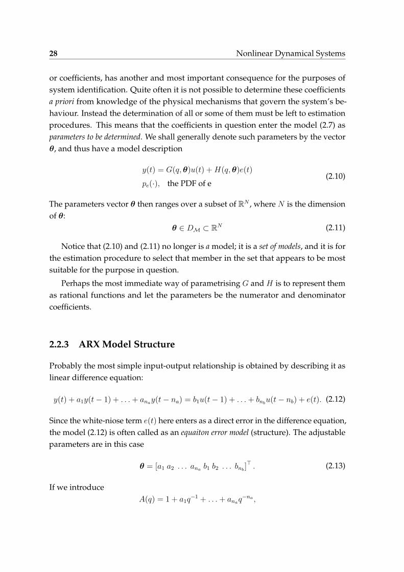
or coefficients, has another and most important consequence for the purposes ofsystem identification. Quite often it is not possible to determine these coefficientsa priori from knowledge of the physical mechanisms that govern the system’s be-haviour. Instead the determination of all or some of them must be left to estimationprocedures. This means that the coefficients in question enter the model (2.7) asparameters to be determined. We shall generally denote such parameters by the vectorθ, and thus have a model description
y(t) = G(q, θ)u(t) + H(q, θ)e(t)pe(·), the PDF of e
(2.10)
The parameters vector θ then ranges over a subset of RN , where N is the dimensionof θ:
θ ∈ DM ⊂ RN (2.11)
Notice that (2.10) and (2.11) no longer is a model; it is a set of models, and it is forthe estimation procedure to select that member in the set that appears to be mostsuitable for the purpose in question.
Perhaps the most immediate way of parametrising G and H is to represent themas rational functions and let the parameters be the numerator and denominatorcoefficients.
2.2.3 ARX Model Structure
Probably the most simple input-output relationship is obtained by describing it aslinear difference equation:
y(t) + a1y(t− 1) + . . . + anay(t− na) = b1u(t− 1) + . . . + bnbu(t− nb) + e(t). (2.12)
Since the white-niose term e(t) here enters as a direct error in the difference equation,the model (2.12) is often called as an equaiton error model (structure). The adjustableparameters are in this case
θ = [a1 a2 . . . ana b1 b2 . . . bnb]⊤ . (2.13)
If we introduceA(q) = 1 + a1q
−1 + . . . + anaq−na ,

2.2 Linear Time-Invariant Systems 29
andB(q) = b1q
−1 + . . . + bnbq−nb .
We see that (2.12) corresponds to (2.10) with
G(q, θ) = B(q)A(q) , H(q, θ) = 1
A(q) . (2.14)
Remark 1 It may seem annoying to use q as an argument of A(q), being a polynomial inq−1. The reason for this is, however, simply to be consistent with the conventional definitionof the z-transform.
2.2.4 ARMAX Model Structure
The basic disadvantage with the simple model (2.12) is the lack of adequate freedomin describing the properties of the disturbance term. We could add flexibility to thatby describing the equation as a moving average of white noise. This gives the model
y(t) + a1y(t− 1) + . . . + anay(t− na)=b1u(t− 1) + . . . + bnb
u(t− nb) + e(t) + c1e(t− 1) + . . . + cnee(t− nc),(2.15)
withC(q) = 1 + c1q
−1 + . . . + cncq−nc .
It can be rewritten asA(q)y(t) = B(q)u(t) + C(q)e(t) (2.16)
and clearly corresponds to (2.7) with
G(q, θ) = B(q)A(q) , H(q, θ) = C(q)
A(q) , (2.17)
where nowθ =
[a1 . . . ana b1 . . . bnb
c1 . . . cnc
]⊤.
In view of the moving average (MA) part C(q)e(t), the model (2.16) will be calledARMAX. The ARMAX model has become a standard tool in control and economet-rics for both system description and control design. A version with an enforcedintegration in the noise description is the ARIMA(X) model (I for integration, with orwithout the X-variable u), which is useful to describe systems with slow disturbance:

30 Nonlinear Dynamical Systems
see the book by Box and Jenkins [25]. It is obtained by replacing y(t) and u(t) in (2.16)by their differences ∆y(t) = y(t)− y(t− 1).
2.2.5 Linear Regression Model
Let us compute the predictor for (2.12), which gives
y(t|θ) = B(q)u(t) + [1− a(q)] y(t) (2.18)
Clearly, this expression could have more easily been derived from (2.12). Withouta stochastic framework, the predictor (2.18) is a natural choice if the the term e(t)in (2.12) is considered to be “insignificant” or “difficult to guess.” It is thus perfectnatural to work with the expression (2.18) also for the “deterministic” models.
Now we introduce the vector
ϕ(t) =[−y(t− 1) . . . −y(t− na) u(t− 1) . . . u(t− nb)
]⊤. (2.19)
Then (2.18) can be rewritten as
y(t|θ) = ϕ(t)⊤θ. (2.20)
This is the important property of (2.12) that we alluded to previously. The predictoris a scalar product between a known data vector ϕ(t) and the parameter vector θ.Such a model is called a linear regression in statistics, and the vector ϕ(t) is knownas the regression vector. It is of importance since powerful and simple estimationmethod can be applied for the determination of θ.
In case some coefficient of the polynomials A and B are known, we arrive at thelinear regression of the form
y(t|θ) = ϕ⊤(t)θ + µ(t) (2.21)
where µ(t) is a known term.
2.3 Nonlinear Time-Invariant Systems
In Eq. (2.21), we defined a linear regression model structure where the prediction islinear in the parameters:
y(t|θ) = ϕ(t)⊤θ. (2.22)

2.3 Nonlinear Time-Invariant Systems 31
To describe a linear difference equation, the components of the vector ϕ(t) (i.e.,the regressors), were chosen as lagged input and output values: see (2.19). Whenusing (2.22) it is, however, immaterial how ϕ(t) is formed: what matters is that it isa known quantity at time t. We can thus let it contain arbitrary transformations ofmeasured data. Let, as usual, yt and ut denote the input and output sequences up totime t. Then we could write
y(t|θ) = θ1ϕ1(ut, yt−1) + . . . + θdϕd(ut, yt−1) = ϕ(t)⊤θ (2.23)
with arbitrary functions ϕ(t) of past data. The structure (2.23) could be regardedas a finite-dimensional parametrisation of a general, unknown, nonlinear predictor.The key is how to choose the functions ϕi(ut, yt−1). Next we will discuss on how tochoose ϕi(ut, yt−1) using polynomial terms.
Example 1 As an example of the above, consider the following model of polynomial termssingle-input single-output (SISO) nonlinear autoregressive system with exogenous inputs(NARX model) [112]
x(t + 1) = 0.7x5(t)x(t− 1)− 0.5x(t− 2) + 0.6u4(t− 2)− 0.7x(t− 2)u2(t− 1) + ξ(t).(2.24)
with x ∈ R, u ∈ R, and ξ ∈ R. The maximal state and input memory orders are mx = 2and mu = 2 respectively.
Suppose we collect M + 2 data samples satisfying (2.24). We can then write the corre-sponding dynamics as
y = Xθ + Ξ
with
y ≜[
x(4), . . . , x(M)]T∈ R(M−3)×1,
X ≜
x5(3)x(2) x(1) u4(1) x(1)u2(2)
......
......
x5(M − 1)x(M − 2) x(M − 3) u4(M − 3) x(M − 3)u2(M − 2)
∈ R(M−3)×4,
θ ≜ [0.7,−0.5, 0.6, 0.7]T ∈ R4×1
Ξ ≜[
ξ(3), . . . , ξ(M − 1)]T∈ R(M−3)×1. (2.25)

32 Nonlinear Dynamical Systems
2.3.1 Nonlinear Time-Invariant Systems
Now we give a formal introduction to the nonlinear time-invariant systems consid-ered in this and next Chapters. With appropriately chosen embedding dimension ormemory of the system κi (resp. νj) for state (resp. input) variable xi (resp. uj), fori = 1, . . . , nx, j = 1, . . . , nu and k = 1, . . . , nξ one can obtain delayed coordinate andNx-dimensional stacked state vector
xi(t) = [xi(t), xi(t− 1), . . . , xi(t− (κi − 1))]⊤ ∈ Rκi ,
X(t) =[(x1(t))⊤, · · · , (xnx(t))⊤
]⊤∈ RNx , Nx =
∑nx
i=1 κi;(2.26)
and delayed coordinate and Nu-dimensional stacked input vector
uj(t) = [uj(t), uj(t− 1), . . . , uj(t− (νj − 1))]⊤ ∈ Rνj ,
U(t) = [(u1(t))⊤, · · · , (unu(t))⊤]⊤ ∈ RNu , Nu =∑nu
j=1 νj.(2.27)
and delayed coordinate and Nξ-dimensional stacked noise vector
ξk(t) = [ξk(t), ξk(t− 1), . . . , ξk(t− (υk − 1))]⊤ ∈ Rυk ,
Ξ(t) = [(ξ1(t))⊤, · · · , (ξnξ(t))⊤]⊤ ∈ RNξ , Nξ =
∑nξ
k=1 υk.(2.28)
Suppose τ is a natural number, the delayed element in xi(t), uj(t) and ξk(t) canbe indexed as xi(t− τ), uj(t− τ) and ξk(t− τ) respectively. τ can be interpreted astemporal index of the data, as well as the sampling interval and delay which can bean arbitrary positive real number. To ease notations and efficient temporal index ofthe data, we assume τ = 1 throughout the thesis. The system dynamics are typicallywritten in the Langevin form and referred to as “the Langevin equation” and thecorresponding observation equations, i = 1, . . . , nx:
xi(t + 1) = Fi (X(t), U(t)) + Gi (X(t), U(t)) ·Ξ(t), (2.29)
zi(t) = xi(t) + ϵi(t), (2.30)
xi(t) is the system or state variable, the observation variable zi(t) is the collected datacontaminated by the ubiquitous observational noise. Similarly, we can define thedelayed coordinate and Nz-dimensional stacked observation vector zi(t) and Z(t).The underlying assumption here is all state variables are observable, i.e., Nz = Nx.In probability and mathematical finance community, Fi is the drift coefficient andGi is the diffusion coefficient.

2.3 Nonlinear Time-Invariant Systems 33
Remark 2 On the left hand side of (2.29), we replace xi(t + 1) with some other quantities,i.e., δ(t, xi(t + 1)). δ(t, xi(t)) can be defined depending whether there is state variable in theexpression. In the state-independent scenario, it can be expressed as a polynomial function oftime t, for example,
δ(t, xi(t + 1)) ≜ t or t2 etc, (2.31a)
δ(t, xi(t + 1)) ≜ log t, t > 0, (2.31b)
δ(t, xi(t + 1)) ≜ constant. (2.31c)
Applications include factor asset pricing models [38], conservation laws in physics andchemistry.
In the state-dependent scenario, to give a few examples in the following, it can be expressedas
δ(t, xi(t + 1)) ≜ xi(t + 1), (2.32a)
δ(t, xi(t + 1)) ≜ xi(t + 1)− xi(t), (2.32b)
δ(t, xi(t + 1)) ≜ log xi(t + 1), xi(t) > 0, (2.32c)
δ(t, xi(t + 1)) ≜ log xi(t + 1)− log xi(t), xi(t), xi(t− τ) > 0. (2.32d)
In particular, when the system can be characterised by differential equations, we have
δ(t, xi(t + 1)) ≜ dxi(t)dt
= xi(t). (2.33)
Remark 3 Here we discuss the identification of continuous system. It should be noted thatcontinuous system can be covered if xi(t) can be obtained or assumed to estimated withconfidence. Otherwise, continuous system identification is not covered in the thesis. Inpractice, estimation of the first derivative data matrix is not a trivial task. After tryingvarious techniques, we decided to use the techniques proposed in [48]. The details willbe given later in Section 5.6. The other issue that needs to be pointed out is how to dealmeasurement noise ϵi(t) in Eq. (2.30). This issue will be discussed later in Section 5.5.
2.3.2 Some Key Assumptions
In all its generality, the formulation in Eq. (2.29) and other variations in Remark 2encompasses a wide variety of networked models in physics, chemistry, biology,engineering, finance and economics.

34 Nonlinear Dynamical Systems
The objective is thus to identify the possibly nonlinear functions Fi (and theirassociated parameters) in (2.29) given measured noisy time series data zi in (2.30)of the state variables xi. However, it’s too ambitious to accomplish the objectivewithout any assumptions. Before proposing our method, some (hopefully) mildassumptions need to be made on the structure form of Fi; estimation or calculation ofleft hand side quantity δ(·, ·); distribution and form of dynamic and/or observationnoise.
We focus on systems where our a priori knowledge about the underlying princi-ples allows us to assume that the model will adopt a concise description in terms ofa set of candidate basis (or dictionary) functions, as is the case in many of the applica-tions of interest in physics, chemistry, biology, engineering, finance and economics.In particular, we make the following key assumption.
Assumption 1 xi(t) in (2.26), uj(t) in (2.27), ξk(t) in (2.28) and ϵi(t) in (2.30) are as-sumed to be bounded and independent with each other for i = 1, . . . , nx, j = 1, . . . , nu andk = 1, . . . , nξ.
Assumption 2 The function Fi(X(t), U(t)) can be represented as linear combinations ofdictionary functions:
φi(X(t), U(t)) ={φin : Rnx+nu → R
}Ni
n=1(2.34)
such that
Fi (X(t), U(t)) =Ni∑
n=1βinφin(X(t), U(t)) := Φ⊤
i (t)βi, (2.35)
where Φ⊤i (t) : RNx+Nu → RNi . It should be noted that some φin may be redundant in this
representation, i.e. βin = 0 accordingly. The set of nx such description vectors
{βi}i=1,...,nx(2.36)
encodes the representation of the full system in terms of the dictionary functions {Φi}.
Remark 4 In Assumption 2, the basis function is assumed to be “linear in parameters”.Though this covers a large class of system, it is still limited for some systems such as (Deep)Neural Networks. Thereafter, we next propose Assumption 3 which is more general thanAssumption 2. However, throughout the thesis, the dynamical systems considered areassumed as stated in Assumption 2 except those of Chapter 7.1 of Part II and future work in

2.3 Nonlinear Time-Invariant Systems 35
14. This Assumption is applied in Chapter 7 where the likelihood with exponential familydistribution.
Now we go beyond the “linear in parameters” restriction and propose the moregeneral Assumption 2.
Assumption 3 The function Fi(X(t), U(t)) can be represented as linear combinations ofdictionary functions:
φi(X(t), U(t), βi) ={φin : Rnx+nu+nβin → R
}Ni
n=1(2.37)
such that
Fi (X(t), U(t)) =Ni∑
n=1φin(X(t), U(t), βin) (2.38)
where βin ∈ Rnβin . The set of∑nx
i=1 Ni such description vectors
{βin}i=1,...,nx,n=1,...,Ni(2.39)
encodes the representation of the full system in terms of the dictionary functions {φi}.
Next we discuss assumptions on the form of the diffusion term in (2.29).
Assumption 4 Given (2.28), the diffusion term in (2.29) can be expressed as
Gi (X(t), U(t)) ·Ξ(t) =nξ∑
k=1
υk−1∑τ=0
gikτ (X(t), U(t)) ξk(t− τ) (2.40)
where gikτ : RNx+Nu → R is an arbitrary bounded function, e.g., zero, monomial, etc. AndGi is bounded as well.
Follow the linear combination representation assumption both in (2.35) and (2.38),another key assumption is on “sparse representation”.
Assumption 5 The sets in (2.36) and (2.39) are sparse (β has many zero elements), andthe representation in (2.35) and (2.38) are sparse as well.
Remark 5 (Assumption 5) This assumption is concise but fundamental in this thesis. Itis relevant to model selection criteria such as Akaike information criterion (AIC) [3] andBayesian information criterion (BIC) [167].

36 Nonlinear Dynamical Systems
We make another key assumption on “full measurement”
Assumption 6 The system (2.29) is fully measurable, i.e., all the state variables xi can bemeasured and there are no hidden variables in the nonlinear system.
Remark 6 (Assumption 6) Typically, only part of the state is measured [224, 223], and,in particular, the number of hidden/unobservable nodes and their position in the networkare usually unknown. Fortunately, this may be problematic only in nonlinear systemidentification but not in linear system identification. However, in economics and financialtime series modelling [122, 203, 198], asset pricing modelling [38] and the seminal paperon Granger causality [68], the model only consist of the measured variables. Meanwhile, in(deep) neural network systems, the model also employs complicated nonlinear embeddingfrom input to output.
To incorporate prior knowledge into the identification problem, it is often im-portant to be able to impose constraints on β. In biological systems, positivity ofthe parameters constituting β is an example of such constraints. The other moti-vation for constrained optimisation comes from stability considerations. Typically,the underlying system is known a priori to be stable, especially if this system is abiological or physical system. A lot of stability conditions can be formulated asconvex optimisation problems, e.g. Lyapunov stability conditions expressed asLinear Matrix Inequalities [26], Gershgorin Theorem for linear systems [89], etc.Only few contributions are available in the literature that address the problem ofhow to consider a priori information on system stability during system identification[34, 229]. To be able to integrate constraints on β into the problem formulation, weconsider the following assumption on β.
Assumption 7 Constraints on the weights β can be described by a set of convex functions:
H[I]i (β) ≤ 0, i = 1, . . . , mI ,
H[E]j (β) = 0, j = 1, . . . , mE.
(2.41)
where the convex functions H[I]i : RN → R are used to define inequality constraints, whereas
the convex functions H[E]j : RN → R are used to define equality constraints.
2.3.3 Linear Regression Model
We first start with a simple model where the next step states only depends on thecurrent step states and/or inputs, i.e. discrete-time MIMO nonlinear systems with

2.3 Nonlinear Time-Invariant Systems 37
additive noise:
x(t + 1) = f(x(t), u(t)) + ξ(t), (2.42)
zi(t) = xi(t), (2.43)
andx = [x1, . . . , xnx ]⊤ ∈ Rnx
denotes the state vector;u = [u1, . . . , unu ]⊤ ∈ Rnu
denotes the input vector;
f(·) ≜ [f1(·), . . . , fnx(·)]⊤ : Rnx+nu → Rnx
denotes the nonlinear functions;
ξ = [ξ1, ξ2, . . . , ξnx ]⊤ ∈ Rnx
denotes the dynamic noise vector, where ξi(t) is assumed to be Gaussian i.i.d. :
ξi(t) ∼ N (0, σ2i )
with
E(ξi(p)) = 0,
E(ξi(p)ξi(q)) = σ2i δpq,
δpq =
1, p = q,
0, p = q.
Under Assumptions 2 and 6, the system in (2.42) can be rewritten into the linearregression form:
xi(t + 1) = f⊤i (x(t), u(t))vi + ξi(t), i = 1, . . . , nx, (2.44)
wherevi = [vi1, . . . , viNi
]⊤ ∈ RNi

38 Nonlinear Dynamical Systems
is the weight vector to be identified and
f⊤i (x(t), u(t)) = [fi1(x(t), u(t)), . . . , fiNi
(x(t), u(t))] ∈ RNi
is the vector of considered dictionary functions (which does not contain unknownparameters).
If data samples satisfying (2.44) can be obtained from the system of interest.When data are sampled, we assume the data matrix and first derivative/differencedata matrix satisfying (2.44) can be obtained as
x1(1) . . . xnx(1)
... . . . ...x1(M) . . . xnx(M)
(2.45)
and x1(2) . . . xnx(2)
... . . . ...x1(M + 1) . . . xnx(M + 1)
(2.46)
respectively. Now we letyi(t) ≜ xi(t + 1),
model (2.42) can be written as
yi = Ψivi + Ξi, i = 1, . . . , nx, (2.47)
withyi ≜ [yi(1), . . . , yi(M)]⊤ ∈ RM×1,
Ψi ≜
fi1(x(1), u(1)) . . . fiNi
(x(1), u(1))... . . . ...
fi1(x(M), u(M)) . . . fiNi(x(M), u(M))
∈ RM×Ni ,
vi ≜ [vi1, . . . , viNi]T ∈ RNi×1,
Ξi ≜ [ξi(1), . . . , ξi(M)]⊤ ∈ RM×1.
(2.48)
We want to find vi given the measured noisy data stored in yi. This is a typical linearregression problem that can be solved using standard least square approaches, pro-vided that the structure of the nonlinearities in the model are known, i.e., providedthat Ψi is known.

2.3 Nonlinear Time-Invariant Systems 39
In what follows we gather in a matrix Xi similar to Ψi the set of all candi-date/possible basis functions. This is an equivalent augmentation of (2.44) byintroducing “redundant” terms with corresponding parameters be zero in the rep-resentation. Due to such expansion of the dictionary matrix, vi will be substitutedby a new parameter vector βi. The issues on the selection of basis functions will bediscussed later in Section 5.2. Now we consider:
yi = Xiβi + Ξi, i = 1, . . . , nx. (2.49)
The solution βi to (2.49) is typically going to be sparse due to the potential introduc-tion of non-relevant and/or non-independent dictionary functions in Xi.
Example 2 As an illustrative example, we consider the following model of polynomial termsfor a single-input single-output (SISO) nonlinear autoregressive system with exogenousinput (NARX model) [112]:
x(t + 1) = 0.7x5(t)x(t− 1)− 0.5x(t− 2) + 0.6u4(t− 2)− 0.7x(t− 2)u2(t− 1) + ξ(t),(2.50)
with x, u, ξ ∈ R. Then we can write an extended form
x(t + 1) = w1 + w2x(t) + . . . + wmx+2x(t−mx) + . . . + wNxdx(t−mx)udu(t−mu) + ξ(t)= β⊤f(x(t), . . . , x(t−mx), u(t), . . . , u(t−mu)) + ξ(t),
where dx (resp. du) is the degree of the output (resp. input); mx (resp. mu) is the maximalmemory order of the output (resp. input); β⊤ = [w1, . . . , wN ] ∈ RN is the weight vector;and
f(x(t), . . . , x(t−mx), u(t), . . . , u(t−mu)) = [f1(·), . . . , fN(·)]⊤ ∈ RN
is the dictionary functions vector. Then for the NARX model (2.50), we can find dx = 5,du = 4, mx = 2, mu = 2. To define the dictionary matrix, we consider all possible monomialsup to degree dx = 5 (resp. du = 4) and up to memory order mx = 5 (resp. mu = 2) in x
(resp. u). which gives f(·) ∈ R1960 thus β ∈ R1960. Since v ∈ R4, only 4 out of the 1960associated weights wi are nonzero.
Since the nx linear regression problems in (2.49) are independent, for simplicityof notation, we omit the subscript i in (2.49) and write
y = Xβ + Ξ. (2.51)

40 Nonlinear Dynamical Systems
As indicated in Example 2, a large number of candidate basis functions can beconsidered to construct X. This means that the number of columns N of X tends tobe very large. Meanwhile, the time-series measurements collected are quite limited.To find the sparsest solution is desirable but NP-hard and numerically unstable.
2.3.4 Additional Experiment Designs
During the identification process, additional experiments can be performed to makethe data set and the data-dependent dictionary matrix more informative for iden-tification (see Sec. 13 of [117]). To ease notation, we assume the same amount ofmeasurements are sampled for each new experiment. The equation with superscript[0] denotes the initial experiment. For simplicity, we consider in particular on thediscrete-time dynamical system
xi(t + 1) = f⊤i (x(t), u(t))vi + ξi(t), i = 1, . . . , nx, (2.52)
Additional Excitation Signals Applied to the Inputs of the System Supposethere are nd different excitation signals u[k], k = 0, . . . , nd, applied to the inputsof the system. We can then expand (2.52) as:
x[0]i (t + 1) = f⊤
i (x[0](t), u[0](t))vi + ξ[0]i (t),
x[1]i (t + 1) = f⊤
i (x[1](t), u[1](t))vi + ξ[1]i (t),
......
x[nd]i (t + 1) = f⊤
i (x[nd](t), u[nd](t))vi + ξ[nd]i (t).
(2.53)
We stack all input and output data together and define
yi ≜
y[0]
i
y[1]i...
y[nd]i
∈ RM ·(nd+1)×1, Ψi ≜
Ψ[0]
i
Ψ[1]i...
Ψ[nd]i
∈ RM ·(nd+1)×Ni ,
vi ≜
vi1...
viNi
∈ RNi×1, Ξi ≜
Ξ[0]
i
Ξ[1]i...
Ξ[nd]i
∈ RM ·(nd+1)×1, (2.54)

2.3 Nonlinear Time-Invariant Systems 41
where
y[j]i ≜
[x
[j]i (1), . . . , x
[j]i (M)
]T∈ RM×1,
Ψ[j]i ≜
fi1(x[j](0), u[j](0)) . . . fiNi
(x[j](0), u[j](0))...
......
fi1(x[j](M − 1), u[j](M − 1)) . . . fiNi(x[j](M − 1), u[j](M − 1))
∈ RM×Ni ,
Ξ[j]i ≜
[ξ
[j]i (0), . . . , ξ
[j]i (M − 1)
]T∈ RM×1.
Using the notation above, system (2.53) can be written as yi = Ψivi + Ξi, i =1, . . . , nx, which has the same form as (2.47).
Perturbation Experiments This case refers to perturbations of the weights vi thatleads to variations in the outputs of the system.1 In this situation, we can write thefollowing equations
x[0]i (t + 1) = f⊤
i (x[0](t), u(t))vi + ξ[0]i (t),
x[1]i (t + 1) = f⊤
i (x[1](t), u(t))(vi + ∆v[1]i ) + ξ
[1]i (t),
......
x[nd]i (t + 1) = f⊤
i (x[nd](t), u(t))(vi + ∆v[nd]i ) + ξ
[nd]i (t).
(2.55)
Similar to the formulation for additional excitation signals applied to the inputs in(2.54), we stack all input and output data and define
yi ≜
y[0]
i
y[1]i...
y[nd]i
∈ RM ·(nd+1)×1, Ψi ≜
Ψ[0]
i 0M×Ni. . . 0M×Ni
Ψ[1]i Ψ[1]
i . . . 0M×Ni
...... . . . ...
Ψ[nd]i 0M×Ni
. . . Ψ[nd]i
∈ RM ·(nd+1)×Ni ,
vi ≜
v[0]
i
∆v[1]i
...∆v[nd]
i
∈ RNi×1, Ξi ≜
Ξ[0]
i
Ξ[1]i...
Ξ[nd]i
∈ RM ·(nd+1)×1, (2.56)
1In molecular biology experiments, this corresponds to the situation where the expression of oneor more of an organism’s genes is reduced through genetic manipulations.

42 Nonlinear Dynamical Systems
where
y[j]i ≜
[x
[j]i (1), . . . , x
[j]i (M)
]T∈ RM×1,
Ψ[j]i ≜
fi1(x[j](0), u(0)) . . . fiNi
(x[j](0), u(0))...
......
fi1(x[j](M − 1), u(M − 1)) . . . fiNi(x[j](M − 1), u(M − 1))
∈ RM×Ni ,
∆v[j]i ≜
[∆v
[j]i1 , . . . , ∆v
[j]iNi
]⊤∈ RNi×1,
Ξ[j]i ≜
[ξ
[j]i (0), . . . , ξ
[j]i (M − 1)
]T∈ RM×1,
and let ∆v[0]i = 0Ni
. Using the notation above, we can again write the formulationas yi = Ψivi + Ξi, i = 1, . . . , nx, which is similar to (2.47).
Knockout Experiment The term “Knockout” comes from “gene knockout” inmolecular biology when certain organism’s genes are knocked out of the organism.If one state variable xj is knocked out, all the dictionary functions that involved xj
will be excluded from the dictionary matrix or set to zero. The model structure andconnections among other state variables will remain unchanged. This also applies tothe deletion of multiple state variables. Recall the definition of the dictionary func-tion vector: fi(x(t), u(t)) = [fi1(x(t), u(t)), . . . , fiNi
(x(t), u(t))]⊤ ∈ RNi , and furtherdefine the subset index Ij ⊂ {1, 2, . . . , n} containing the indices of the knocked out
variables during knockout experiment j. f[I−
j ]i (·) denotes the vector/matrix formed
by the elements/columns of fi(·) with indices in Ij set to zeros. The data collectedthrough knockout experiments can then be seen to satisfy the following equations
x[0]i (t + 1) = f [I−
0 ]i
⊤(x[0](t), u[0](t))vi + ξ
[0]i (t),
x[1]i (t + 1) = f [I−
1 ]i
⊤(x[1](t), u[1](t))vi + ξ
[1]i (t),
......
x[nd]i (t + 1) = f [I−
nd]
i
⊤(x[nd](t), u[nd](t))vi + ξ
[nd]i (t).
(2.57)

2.3 Nonlinear Time-Invariant Systems 43
Similar to the formulation for additional excitation signals in (2.54) and perturbationexperiments in (2.56), we stack all input and output data and define
yi ≜
y[0]
i
y[1]i...
y[nd]i
∈ RM ·(nd+1)×1, Ψi ≜
Ψ[I−0 ]
i
Ψ[I−1 ]
i...
Ψ[I−nd
]i
∈ RM ·(nd+1)×Ni ,
vi ≜
vi1...
viNi
∈ RNi×1, Ξi ≜
Ξ[0]
i
Ξ[1]i...
Ξ[nd]i
∈ RM ·(nd+1)×1, (2.58)
where
y[j]i ≜
[x
[j]i (1), . . . , x
[j]i (M)
]T∈ RM×1,
Ψ[I−
j ]i ≜
fi1(x[j](0), u[j](0)) . . . fiNi
(x[j](0), u[j](0))...
......
fi1(x[j](M − 1), u[j](M − 1)) . . . fiNi(x[j](M − 1), u[j](M − 1))
∈ RM×Ni ,
Ξ[j]i ≜
[ξ
[j]i (0), . . . , ξ
[j]i (M − 1)
]T∈ RM×1.
It should be noted that certain columns of Ψ[I−
j ]i indexed by Ij would be zero columns.
Again, using the above notation, we obtain the formulation yi = Ψivi + Ξi, i =1, . . . , nx, which has the same form as (2.47).
Remark 7 From the above analysis, we can re-formulate the data coming from the additionalexperiments (replicates, perturbation, knock-out) to the standard form yi = Ψivi + Ξi (withdifferent matrix dimensions). In the next Section, we shall propose a solution to suchproblems.
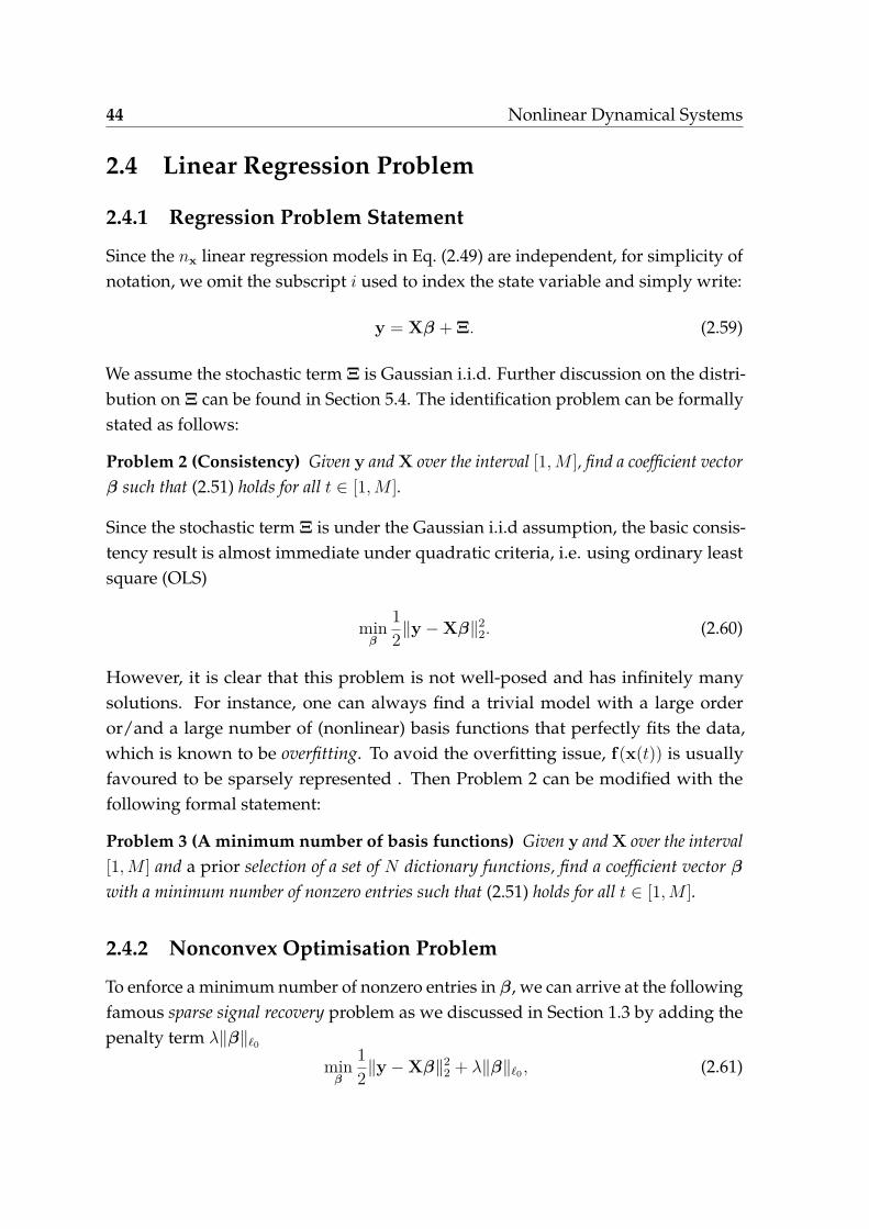
44 Nonlinear Dynamical Systems
2.4 Linear Regression Problem
2.4.1 Regression Problem Statement
Since the nx linear regression models in Eq. (2.49) are independent, for simplicity ofnotation, we omit the subscript i used to index the state variable and simply write:
y = Xβ + Ξ. (2.59)
We assume the stochastic term Ξ is Gaussian i.i.d. Further discussion on the distri-bution on Ξ can be found in Section 5.4. The identification problem can be formallystated as follows:
Problem 2 (Consistency) Given y and X over the interval [1, M ], find a coefficient vectorβ such that (2.51) holds for all t ∈ [1, M ].
Since the stochastic term Ξ is under the Gaussian i.i.d assumption, the basic consis-tency result is almost immediate under quadratic criteria, i.e. using ordinary leastsquare (OLS)
minβ
12∥y−Xβ∥2
2. (2.60)
However, it is clear that this problem is not well-posed and has infinitely manysolutions. For instance, one can always find a trivial model with a large orderor/and a large number of (nonlinear) basis functions that perfectly fits the data,which is known to be overfitting. To avoid the overfitting issue, f(x(t)) is usuallyfavoured to be sparsely represented . Then Problem 2 can be modified with thefollowing formal statement:
Problem 3 (A minimum number of basis functions) Given y and X over the interval[1, M ] and a prior selection of a set of N dictionary functions, find a coefficient vector β
with a minimum number of nonzero entries such that (2.51) holds for all t ∈ [1, M ].
2.4.2 Nonconvex Optimisation Problem
To enforce a minimum number of nonzero entries in β, we can arrive at the followingfamous sparse signal recovery problem as we discussed in Section 1.3 by adding thepenalty term λ∥β∥ℓ0
minβ
12∥y−Xβ∥2
2 + λ∥β∥ℓ0 , (2.61)

2.4 Linear Regression Problem 45
where λ is the regularisation parameter.
2.4.3 Convex Relaxation
Again, as we discussed in Chapter 1.3, we replace ∥β∥ℓ0 in the optimisation aboveby ∥β∥ℓ1 . The idea behind this relaxation is the fact that the ℓ1 norm is the convexenvelope of the ℓ0 norm, and thus, in a sense, minimising the former yields the bestconvex relaxation to the (non-convex) problem of minimizing the latter. It gives
minβ
12∥y−Xβ∥2
2 + λ∥β∥ℓ1 . (2.62)
Remark 8 We notice that there is a hyperparameter λ which needs to be specified a priorior tuned manually. λ is known as regularisation parameter. The selection of optimalregularisation parameter is an open problem in machine leaning and statistics and hasbeen discussed in any machine learning textbook. Without otherwise specified, we usecross-validation for choice of the optimal λ [22, 79, 127].


Chapter 3
Nonlinear Dynamical System withHeterogeneous Datasets
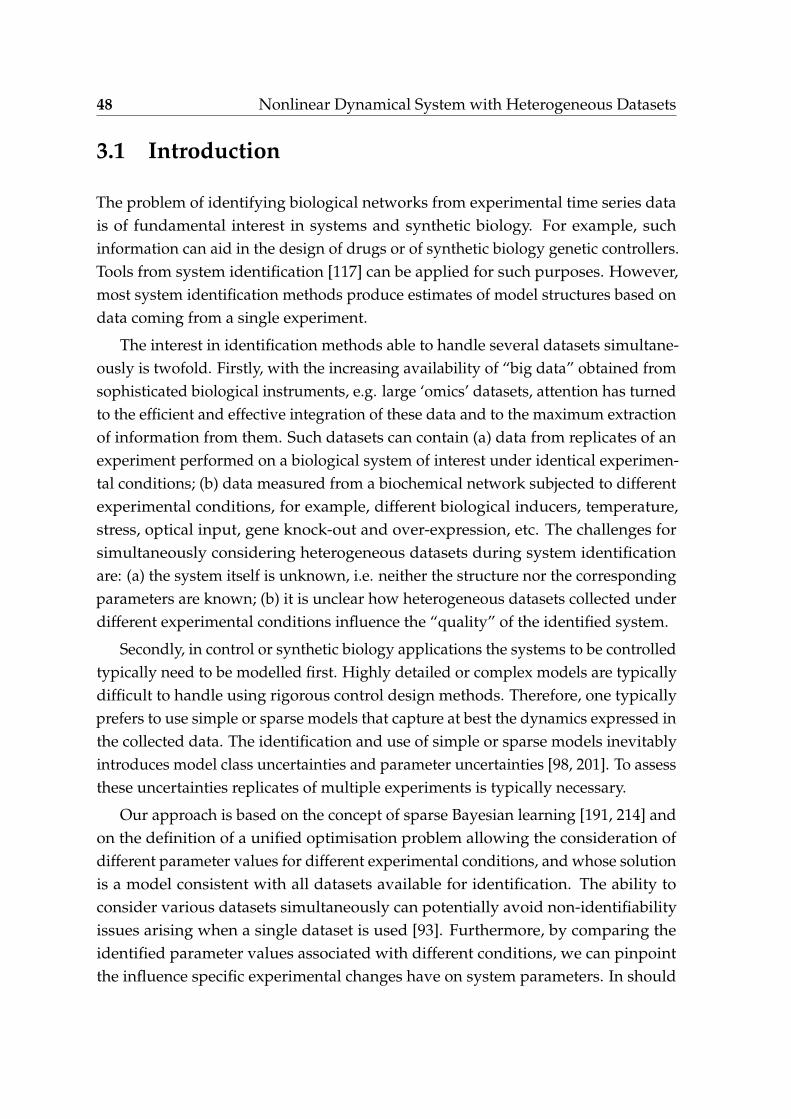
48 Nonlinear Dynamical System with Heterogeneous Datasets
3.1 Introduction
The problem of identifying biological networks from experimental time series datais of fundamental interest in systems and synthetic biology. For example, suchinformation can aid in the design of drugs or of synthetic biology genetic controllers.Tools from system identification [117] can be applied for such purposes. However,most system identification methods produce estimates of model structures based ondata coming from a single experiment.
The interest in identification methods able to handle several datasets simultane-ously is twofold. Firstly, with the increasing availability of “big data” obtained fromsophisticated biological instruments, e.g. large ‘omics’ datasets, attention has turnedto the efficient and effective integration of these data and to the maximum extractionof information from them. Such datasets can contain (a) data from replicates of anexperiment performed on a biological system of interest under identical experimen-tal conditions; (b) data measured from a biochemical network subjected to differentexperimental conditions, for example, different biological inducers, temperature,stress, optical input, gene knock-out and over-expression, etc. The challenges forsimultaneously considering heterogeneous datasets during system identificationare: (a) the system itself is unknown, i.e. neither the structure nor the correspondingparameters are known; (b) it is unclear how heterogeneous datasets collected underdifferent experimental conditions influence the “quality” of the identified system.
Secondly, in control or synthetic biology applications the systems to be controlledtypically need to be modelled first. Highly detailed or complex models are typicallydifficult to handle using rigorous control design methods. Therefore, one typicallyprefers to use simple or sparse models that capture at best the dynamics expressed inthe collected data. The identification and use of simple or sparse models inevitablyintroduces model class uncertainties and parameter uncertainties [98, 201]. To assessthese uncertainties replicates of multiple experiments is typically necessary.
Our approach is based on the concept of sparse Bayesian learning [191, 214] andon the definition of a unified optimisation problem allowing the consideration ofdifferent parameter values for different experimental conditions, and whose solutionis a model consistent with all datasets available for identification. The ability toconsider various datasets simultaneously can potentially avoid non-identifiabilityissues arising when a single dataset is used [93]. Furthermore, by comparing theidentified parameter values associated with different conditions, we can pinpointthe influence specific experimental changes have on system parameters. In should

3.2 Linear Regression Model 49
be noted that there are similarities between our approach to nonlinear randomeffects models and recent work in the area of generalized linear models (GLIM) forlongitudinal data (e.g., Stiratelli et al., 1984; Liang and Zeger, 1986).
In this Chapter, we will extend the regression model in Chapter 2, to deal withmultiple datasets. In Section 3.2, we will give the regression problem formulation forthe nonlinear SYSID problem from multiple experiments. The regression problem isfurther formulated as a ℓ0 type optimisation problem in Section 3.3.2 and a tentativeempirical ℓ1 relaxation is proposed in Section 3.3.3. The algorithms for this Chapterwill be provided in Section 6.7 of Chapter 6.
3.2 Linear Regression Model
In Section 2.3.3, we introduced the linear regression model in (2.49) for single datasetmodelling. Suppose a total number of C datasets are collected from C independentexperiments, we put a subscript [c] to index the identification problem associatedwith the specific dataset obtained from experiment [c]. The linear regression problem(2.49) for single dataset can be rewritten as
y[c] = X[c]β[c] + ξ[c], c = 1, . . . , C, (3.1)
in which,X[c] ≜
[X[c]
:,1, . . . , X[c]:,N
]
=
f1(x[c](1)) . . . fN(x[c](1))
......
f1(x[c](M [c])) . . . fN(x[c](M [c]))
∈ RM [c]×N ,
β[c] ≜[w
[c]1 , . . . , w
[c]N
]⊤∈ RN ,
ξ[c] ≜[ξ[c](1), . . . , ξ[c](M [c])
]⊤∈ RM [c]
,
(3.2)
where x[c](t) =[x
[c]1 (t), . . . , x[c]
nx(t)]∈ Rnx is the state vector at time instant t. It
should be noted that N , the number of basis functions or number of columns of thedictionary matrix X[c] ∈ RM [c]×N , can be very large. Without loss of generality, weassume M [1] = · · · = M [C] = M . The solution to β[c] to (3.1) is typically going to besparse, which is mainly due to the potential introduction of non-relevant and/ornon-independent basis functions in X[c].

50 Nonlinear Dynamical System with Heterogeneous Datasets
y[1]
...y[C]
=
X[1]
:,1 . . . X[1]:,N
. . .X[C]
:,1 . . . X[C]:,N
︸ ︷︷ ︸
C Blocks
β[1]
...β[C]
+
ξ[1]
...ξ[C]
=
X[1]
:,1 X[1]:,N
. . . . . . . . .X[C]
:,1 X[C]:,N
︸ ︷︷ ︸
N Blocks
w[1]1...
w[C]1...
w[1]N...
w[C]N
+
ξ[1]
...ξ[C]
=[
X1 · · · XN
] β1...
βN
+
ξ[1]
...ξ[C]
.
(3.3)
To ensure reproducibility, experimentalists repeat their experiments under thesame conditions, and the collected data are then called “replicates”. Typically,only the average value over these replicates is used for modelling or identificationpurposes In this case, however, only the first moment is used and informationprovided by higher order moments is lost. Moreover, when data originate fromdifferent experimental conditions, it is usually very hard to combine the datasets intoa single identification problem. This Section will address these issues by showinghow several datasets can be combined to define a unified optimisation problemwhose solution is an identified model consistent with the various datasets availablefor identification.
To consider heterogeneous datasets in one single formulation, we stack the vari-ous equations in (3.1) (see Eq. (3.3)). Each stacked equation in Eq. (3.3) correspondsto a replicate or an experiment performed by changing the experimental conditionson the same system.
In Eq. (3.3), for n = 1, . . . , N ,
Xn = blkdiag[X[1]:,n, . . . , X[C]
:,n ], βn = [w[1]n , . . . , w[C]
n ]⊤.
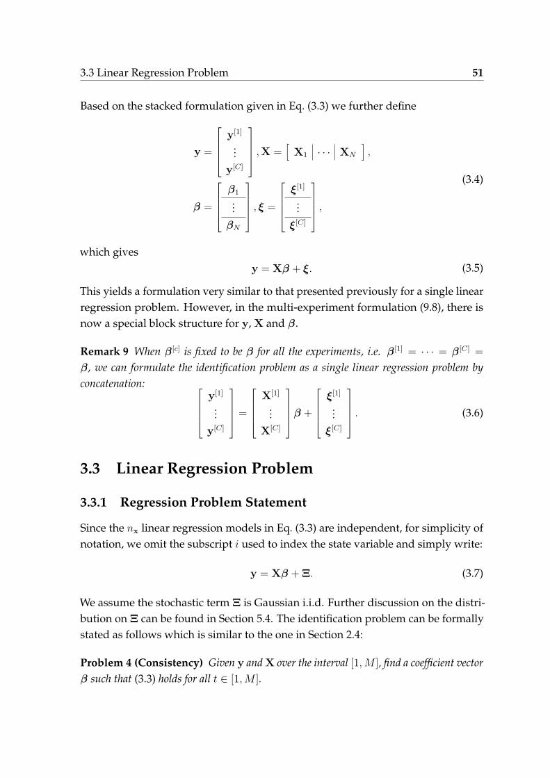
3.3 Linear Regression Problem 51
Based on the stacked formulation given in Eq. (3.3) we further define
y =
y[1]
...y[C]
, X =[
X1 · · · XN
],
β =
β1...
βN
, ξ =
ξ[1]
...ξ[C]
,
(3.4)
which givesy = Xβ + ξ. (3.5)
This yields a formulation very similar to that presented previously for a single linearregression problem. However, in the multi-experiment formulation (9.8), there isnow a special block structure for y, X and β.
Remark 9 When β[c] is fixed to be β for all the experiments, i.e. β[1] = · · · = β[C] =β, we can formulate the identification problem as a single linear regression problem byconcatenation:
y[1]
...y[C]
=
X[1]
...X[C]
β +
ξ[1]
...ξ[C]
. (3.6)
3.3 Linear Regression Problem
3.3.1 Regression Problem Statement
Since the nx linear regression models in Eq. (3.3) are independent, for simplicity ofnotation, we omit the subscript i used to index the state variable and simply write:
y = Xβ + Ξ. (3.7)
We assume the stochastic term Ξ is Gaussian i.i.d. Further discussion on the distri-bution on Ξ can be found in Section 5.4. The identification problem can be formallystated as follows which is similar to the one in Section 2.4:
Problem 4 (Consistency) Given y and X over the interval [1, M ], find a coefficient vectorβ such that (3.3) holds for all t ∈ [1, M ].

52 Nonlinear Dynamical System with Heterogeneous Datasets
Since the stochastic term Ξ is under the Gaussian i.i.d assumption, the basic consis-tency result is almost immediate under quadratic criteria, i.e. using ordinary leastsquare (OLS)
minβ
12∥y−Xβ∥2
2. (3.8)
However, it is clear that this problem is not well-posed and has infinitely manysolutions. For instance, one can always find a trivial model with a large orderor/and a large number of (nonlinear) basis functions that perfectly fits the data,which is known to be overfitting. The “sparse” idea will be again used to avoidoverfitting issue. However, a slightly differently from the strategy proposed inSection 2.4, the Problem 4 can be modified with the following formal statement:
Problem 5 (A minimum number of basis functions) Given y and X over the interval[1, M ] and a prior selection of a set of N dictionary functions, find a coefficient vector β
with a minimum number of basis functions such that (3.3) holds for all t ∈ [1, M ].
3.3.2 Nonconvex Optimisation Problem
To achieve a minimum number of basis functions, we will try to find a coefficientvector β = [β1, . . . , βN ]⊤ with a minimum number of nonzero blocks βi, ∀i =1, . . . , N such that (3.3) holds for all t ∈ [1, M ]. We can arrive at the followingregularised regression problem
minβ
12∥y−Xβ∥2
2 + λN∑
n=1∥∥βn∥ℓ2∥ℓ0 , (3.9)
where λ is the regularisation parameter.
The penalty term ∥∥βi∥ℓ2∥ℓ0 seems a bit complicated, we will give some explana-tions. Since βn = [w[1]
i , . . . , w[C]n ]⊤, for n = 1, . . . , N , we have
∥βn∥ℓ2 =√
(w[1]n )2 + . . . + (w[C]
n )2, (3.10)
it means ∥βi∥ℓ2 = 0 if and only if w[c]i = 0, ∀c = 1, . . . , C. Therefore,
∑Ni=1 ∥∥βi∥ℓ2∥ℓ0
counts the number of basis functions.

3.3 Linear Regression Problem 53
3.3.3 Convex Relaxation
Again, similar as we discussed in Section 2.4.3, we replace ∥∥βn∥ℓ2∥ℓ0 in the optimisa-tion above by ∥∥βn∥ℓ2∥ℓ1 = ∥βi∥ℓ2 . The idea behind this relaxation is the fact that theℓ1 norm is the convex envelope of the ℓ0 norm, and thus, in a sense, minimising theformer yields the best convex relaxation to the (non-convex) problem of minimizingthe latter. It gives
minβ
12∥y−Xβ∥2
2 + λN∑
n=1∥βn∥ℓ2 , (3.11)
This minimisation problem is known as Group Lasso.


Chapter 4
Time-Varying Dynamical System

56 Time-Varying Dynamical System
4.1 Introduction
Identification of switched systems, which are characterised by the interaction of bothcontinuous and discrete dynamics, is widely used in many different fields such assystems/synthetic biology, econometrics, finance, biochemical engineering, socialnetworks, etc. In this Section, we are interested in the identification of regime switchdynamical systems. Biochemical processes can go through different phases in time;for example, a cell cycle in bacteria or diurnal alternations in plants. These switchesare typically triggered by time dependent processes or by some external force.Therefore, the dynamics of biochemical reactions can be modelled as a collectionof submodels amongst which switches occur over time. For biochemical reactionnetworks, the submodels are typically nonlinear due to mass action kinetics.
In classical switched system identification, the submodels are typically assumedto be linear or of the switch affine type [144], which is often used to approximatenonlinear dynamics. In [132], the structure of submodels is fixed and a minimalnumber of switches between submodels is inferred. However, these techniques arenot generally applicable to biochemical kinetics due to highly nonlinear terms andmodel complexity. In the nonlinear case, there is an additional problem of nonlinearbasis selection, which is fixed and predefined in the linear case. Unlike the linearcase, the number of nonlinear basis functions can be infinite and one might have touse complicated nonlinear functions to model the dynamics without any switches.In practice, if one is interested in obtaining the least number of switches, the numberof nonlinear basis functions will typically grow, and vice versa, a small number ofnonlinear basis functions will result in many switches. Hence there are two differentand competing minimisation criteria: the number of switches between submodelsand the number of basis functions in each submodel.
In the first part of this Chapter, we will extend the regression model in Chapter 2and 3, to deal with time-varying systems. In Section 4.3, we will give the regressionproblem formulation for the nonlinear SYSID problem of time-varying systems.The regression problem is further formulated as a ℓ0 type optimisation problem byminimising the number of parameters and the number of switches in Section 4.4.2.A tentative empirical ℓ1 relaxation is proposed in Section 4.4.3. The algorithms forthis Chapter will be provided in Section 6.8 of Chapter 6.
In the second part of the Chapter, we revisit the problem of trend filtering

4.2 Regime-Switch Dynamical System 57
4.2 Regime-Switch Dynamical System
4.2.1 Scalar Linear Regime-Switch Systems
Without loss of generality and to ease notations, we will consider switched autore-gressive exogenous (SARX) hybrid affine models with single input and single output(SISO-SARX) of the form:
y(t) =na∑i=1
ai(αt)y(t− i) +nb∑
i=1bi(αt)u(t− i) + f(αt) + η(t) (4.1)
where u, y and η denote the input, output, and noise, respectively, and wheret ∈ [t0, T ]. The discrete variable αt ∈ {1, . . . , s} - the mode of the system - indicateswhich of the s submodels is active at time t. The time instants where the value of αt
changes are called discrete transitions or switches. These switches partition the interval[0, M ] into a discrete hybrid time set [121], τ = {Ii}k
i=0, such that αt is constant withineach subinterval Ii = [τi, τ ′
i ] and different in consecutive intervals. In the sequel, wedenote by τi and τ ′
i the beginning and ending times of the i-th interval, respectively.Clearly, τ satisfies
• τ0 = 01, and τ ′k = M ,
• τi ≤ τ ′i = τi+1 − 1,
and the number of switches is equal to k.
An equivalent representation of is in the following linear regression form
y(t) = ϕ⊤(t)θ(αt) + η(t) (4.2)
where the regressor vector is
ϕ⊤ =[y(t− 1), . . . , y(t− na), u(t− 1), . . . , u(t− nb) 1
]and the unknown coefficient vector at time t is
θ(αt) =[a1(αt), . . . , ana(αt), b1(αt), . . . , bnb
(αt), f(αt)]
1Since it is not possible to deduce information for t < max(na, nb) when the initial condition areunknown, in the identification problem we take t0 = max(na, nb)

58 Time-Varying Dynamical System
4.2.2 Multivariate Regime-Switch Nonlinear Systems
As we have done in Chapter 2, for nonlinear multivariate hybrid systems, subsys-tems are modelled by nonlinear function for the i-th state variable.
δ(xi(t)) = fαt (x(t), . . . , x(t− na), u(t), . . . , u(t− nb)) + ξ(t), (4.3)
where t ∈ [t0, M ]. δ(·) is defined as in (2.29) The discrete variable αt ∈ {1, . . . , s} -the mode of the system - indicates which of the s submodels is active at time instantt. The time instants where the value of αt changes are call discrete transitions orswitches. These switches partition the interval [0, M ] into a discrete hybrid time set[121], τ = {Ii}k
i=0, such that αt is constant within each subinterval Ii = [τi, τ ′i ] and
different in consecutive intervals. In the sequel, we denote by τi and τ ′i the beginning
and ending times of the i-th interval, respectively. Clearly, τ satisfies
• τ0 = 0, and τ ′k = M ,
• τi ≤ τ ′i = τi+1 − 1,
and the number of switches is equal to k.We assume fαt(·) can be expanded as a linear combination of finite basis functions.
Formally, similar as Assumption 2, we have
Assumption 8 The function terms fαt(·) in (4.3) can be represented as a linear combina-tions of several dictionary functions:
fαt(·) =N∑
i=1θi(αt)fi(·), (4.4)
where θi(αt) ∈ R and fi(x(t)) : Rna+∑m
i=1 nbi → Rnx are smooth functions that are assumedto govern the dynamics.
For simplicity, we let na = 0 and input u = 0. By letting
y(t) = δ(xi(t))
and under Assumption 8, an equivalent linear regression model of (4.3) is
y(t) =(f1(x(t)) . . . fN(x(t)
)· βαt + ξ(t), (4.5)
where fj(x(t) : Rna+∑m
i=1 nbi → Rnx .

4.3 Linear Regression Model 59
Denote Ii is a subset of τ = {Ii}ki=0. And Ii ∩ Ij = ∅, ∀i = j and I1 ∪ . . . ∪ Is = τ .
The discrete transition αt depends on the time instant t, i.e.
fαt(x) =
f1(x) =
(f1(x(t)) . . . fN(x(t)
)· β1, if t ∈ I1
......
fs(x) =(f1(x(t)) . . . fN(x(t)
)· βs, if t ∈ Is
. (4.6)
In each mode, the submodel fj is a smooth function. Therefore, the underlyingassumption on models with the number of switches s is relatively small
s ≤ k ≪M. (4.7)
4.3 Linear Regression Model
Define the following block matrix and vectors, for i = 1, . . . , nx
yi ≜ [y(1), . . . , y(M)]⊤ ,
Xi ≜
f1(x(1)) · fN(x(1))
. . . . . . . . .
f1(x(M)) · fN(x(M))
=[
A1 . . . AN
]∈ RM×MN ,
βi ≜[
βi1(1), . . . , βi1(M) . . . βiN(1), . . . , βiN(M)]⊤
=[
β⊤i1 . . . β⊤
iN
]⊤∈ RMN ,
Ξi ≜ [ξ(1), . . . , ξ(M)]⊤ ∈ RM .
(4.8)
It should be noted that the stochastic term is Gaussian i.i.d with covariance matrixσ2I. We can then formulate the following linear regression problem
yi = Xiβi + Ξi. (4.9)
There are two issues that need to be considered at this stage. First, each blockβin = [win(1), . . . , win(M)] is associated only with certain dictionary function. Thesolution βi to (4.9) is therefore typically going to be block sparse, which is mainlydue to the potential introduction of non-relevant and/or non-independent basisfunctions in X. Second, in the switched case, we have to penalise the number of

60 Time-Varying Dynamical System
switches from t1 to tM and/or the number of modes Nmodes, which can be fixedin advance or set equal to M . Clearly such a problem has an infinite number ofsolutions, especially in the noisy setting. Therefore, we refine the problem statementto identify the system (4.9) with the least number of non-zero entries in βi and theleast number of switches in the sequence αt.
These are actually two different and competing criteria: if we want the leastnumber of switches, the number of non-zero parameters in βi will grow, and viceversa, a small number of non-zero parameters in βi will result in many switches.
4.4 Linear Regression Problem
4.4.1 Regression Problem Statement
Since the nx linear regression models in Eq. (4.8) are independent, for simplicity ofnotation, we omit the subscript i used to index the state variable and simply write:
y = Xβ + Ξ. (4.10)
We assume the stochastic term Ξ is Gaussian i.i.d. Further discussion on the distri-bution on Ξ can be found in Section 5.4. The identification problem can be formallystated as follows which is similar to the one in Section 2.4 and 3.3:
Problem 6 (Consistency) Given y and X over the interval [1, M ], find a coefficient vectorβ such that (4.9) holds for all t ∈ [1, M ].
Since the stochastic term Ξ is under the Gaussian i.i.d assumption, the basic consis-tency result is almost immediate under quadratic criteria, i.e. using ordinary leastsquare (OLS)
minβ
12∥y−Xβ∥2
2. (4.11)
It is clear that this problem is not well-posed and has infinitely many solutions. Forinstance, one can always find a trivial piecewise affine model with M submodelsor on model with a large order or/and a large number of (nonlinear) dictionaryfunctions that perfectly fits the data, which is known to be overfitting. This situationcan be partially avoided by imposing upper bounds ny and nui
, i = 1, . . . , m, on theorder of each of the terms on the right hand side of (4.3), e.g., na ≤ ny, nci
≤ nui.
Still, even in this case the problem admits multiple solutions, especially when ny

4.4 Linear Regression Problem 61
and nuiare very large. More interesting problems can be posed by using the existing
degrees of freedom to optimise suitable performance criteria. One such criterionis to minimise the number of switches (i.e., the minimum number of k), subject toconsistency. Under this criterion, the hybrid system is better characterised by (4.6),where s ≤ k ≪ M.. The formal statement of the identification problem with thiscriterion is as follows:
Problem 7 (A minimum number of switches) Given y and X over the interval [1, M ]and a prior selection of a set of N basis functions, find a coefficient vector β as in (4.8) witha minimum number of switches, such that (4.9) holds for all t ∈ [1, M ].
To further avoid the overfitting issue, fαt(x(t)) is usually favoured to be sparselyrepresented, like we discussed in the previous Chapters. Thus other criterion isto minimise number of same type of dictionary functions. Then Problem 6 can bemodified with the following formal statement:
Problem 8 (A minimum number of basis functions) Given y and X over the interval[1, M ] and a prior selection of a set of N basis functions, find a coefficient vector β as in (4.8)with minimum number of basis functions, such that (4.9) holds for all t ∈ [1, M ].
Now we can consider Problem 7 and Problem 8 simultaneously and state that
Problem 9 Given y and X and the block partitions formulated in (4.9), find a β that canexplain the data with the minimal number of switches and the minimal number of non-zeroblocks in β.
4.4.2 Nonconvex Optimisation Problem
If we index the vector β appropriately, the problem of minimising the numberof switches can be formulated by enforcing Dnβn sparse, where the matrix Dn isdefined as follows:
Dn ≜
1 −1
. . . . . .
1 −1
∈ R(M−1)×M . (4.12)
Problem 7 can be formulated as follows
minβ
12∥y−Xβ∥2
2 + λ1
N∑n=1∥Dnβn∥ℓ0 , (4.13)

62 Time-Varying Dynamical System
where λ1 in (4.13) is the regularisation parameter in this penalised linear regressionproblems.
Considering β =[
β⊤1 . . . β⊤
N
]⊤as in (4.8) is block-wise defined, the problem
of minimising the number of basis functions can be formulated by enforcing β with aminimum number of nonzero blocks βn, n = 1, . . . , N , Problem 8 can be formulatedas follows
minβ
12∥y−Xβ∥2
2 + λ2
N∑n=1∥∥βn∥ℓ2∥ℓ0 , (4.14)
Since∥βn∥ℓ2 ≤ ∥βn∥ℓ1 ,
we can have a bit more ambitious target
minβ
12∥y−Xβ∥2
2 + λ2
N∑n=1∥∥βn∥ℓ1∥ℓ0 , (4.15)
Here we may prefer (4.14) to (4.15) since the former has clearer interpretation in thedynamical model and less computation challenge than (4.15).
Based on the formulation in (4.13) and (4.14) , we can have the following regres-sion problem for Problem 9
minβ
12∥y−Xβ∥2
2 + λ1
N∑n=1∥Dnβn∥ℓ0 + λ2
N∑n=1∥∥βn∥ℓ2∥ℓ0 , (4.16)
The first regulariser λ1∑N
n=1 ∥Dnβn∥ℓ0 penalise the number of switches that occur;and the second regulariser λ2
∑Nn=1 ∥∥βn∥ℓ2∥ℓ0 the number of non-zero element in
every identified model.
4.4.3 Convex Relaxation
Again, similar as we discussed in Section 2.4.3 and 3.3.3, we replace the ℓ0 with ℓ1
in the optimisation problem (4.13), (4.14) and (4.25), we can reach to the followingempirical convex relaxations. For (4.13), the relaxation is
minβ
12∥y−Xβ∥2
2 + λ1
N∑n=1∥Dnβn∥ℓ1 . (4.17)
4.5 Models with Abrupt Change 63
or we can write in a more compact form by defining
D = blkdiag (D1, . . . , DN) , (4.18)
asmin
β
12∥y−Xβ∥2
2 + λ1∥Dβ∥ℓ1 . (4.19)
For (4.14), the relaxation is
minβ
12∥y−Xβ∥2
2 + λ2
N∑n=1∥∥βn∥ℓ2∥ℓ1 , (4.20)
or
minβ
12∥y−Xβ∥2
2 + λ2
N∑n=1∥βn∥ℓ2 . (4.21)
For (4.16), the relaxation is
minβ
12∥y−Xβ∥2
2 + λ1
N∑n=1∥Dnβn∥ℓ1 + λ2
N∑n=1∥βn∥ℓ2 (4.22)
Algorithms minimising the number of non-zero elements and the number ofswitches, i.e. (4.22), belong to the class of so-called fused Lasso algorithms [189]. Forgeneral D matrices, the problem defined in (4.19) and (4.22) would be solved usinggeneralised Lasso algorithms [190].
4.5 Models with Abrupt Change
4.5.1 Trend Filtering
We are given a scalar time series y(t), t = 1, . . . , M , assumed to consist of an under-lying slowly varying trend β(t). The problem we want to solve is to estimate therandom component z(t) = y(t) − β(t). This can be considered as an optimisationproblem with two competing objectives: we want β(t) to be smooth, and we wantz(t) (our estimate of the random component, sometimes called the residual), to besmall. In some contexts, estimating β(t) is called smoothing or filtering.
In [101], an ℓ1 trending filter is proposed and a comprehensive review on thestate-of-art of trend filtering is introduced. Trend filtering comes up in severalapplications and settings including macroeconomics (e.g., [87, 172]), geophysics (e.g.,[13, 23, 24]), financial time series analysis (e.g., [198]), social sciences (e.g., [114]),

64 Time-Varying Dynamical System
revenue management (e.g., [186]), and biological and medical sciences (e.g., [71, 115]).Many trend filtering methods have been proposed, including Hodrick-Prescott (H-P) filtering [87, 113], moving average filtering [131], exponential smoothing [120],bandpass filtering [37, 18], smoothing splines [160], de-trending via rational square-wave filters [157], a jump process approach [236], median filtering [206], a linearprogramming (LP) approach with fixed kink points [126], and wavelet transformanalysis [42]. (All these methods except for the jump process approach, the LPapproach, and median filtering are linear filtering methods; see [18] for a surveyof linear filtering methods in trend estimation.) The most widely used methodsare moving average filtering, exponential smoothing, and H-P filtering, which isespecially popular in economics and related disciplines since its application tobusiness cycle theory [87]. The idea behind H-P filtering can be found in severalfields, and can be traced back at least to work in 1961 by Leser [113] in statistics.
Let’s revisit the optimisation problem in (4.13), when X is the identity matrix IN ,and D is like second difference. Hereafter, we introduce the “sparsest” version ofthe trend filter problem, i.e.,
minβ
12∥y− β∥2
2 + λ∥Dβ∥ℓ0 , (4.23)
where
D ≜
1 −2 −1
. . . . . . . . .
1 −2 1
∈ R(M−2)×M . (4.24)
For what follows, it is useful and clearer to rewrite (4.23) in the following equivalentform:
minβ
12
M∑t=1∥y(t)− β(t)∥2
2 + λM−1∑t=2∥β(t− 1)− 2β(t) + β(t + 1)∥ℓ0 , (4.25)
where β(t) is the trend estimate; λ ≥ is the regularisation parameter used to controlthe trade-off between the smoothness of β(t) and the size of residual y(t)− β(t). Thefirst term in the objective function measures the size of the residual; the second termmeasures the smoothness of the estimated trend. The argument appearing in thesecond term, β(t− 1)− 2β(t) + β(t + 1), is the second difference of the time series attime t; it is zero when and only when the three points β(t− 1), β(t) and β(t + 1) areon a line.In other words, the secondterm in the objective is zero if and only if β(t) is
4.5 Models with Abrupt Change 65
affine, i.e., has the form β(t) = a + bt for some constants a and b. (In other words,the graph of β(t)) is a straight line.)
For the problem (4.25), two convex relaxation strategies can be employed. Thefirst one is to replace ℓ0 norm penalty with a “sum of square” norm term
minβ
12∥y− β∥2
2 + λ∥Dβ∥2ℓ2 , (4.26)
This optimisation problem (4.26) is strictly convex and coercive in β, and so has aunique minimiser. The ℓ2 relaxation is known as the Hodrick-Prescott (H-P) filter.The H-P filter is supported in several standard software packages for statistical dataanalysis, e.g., SAS, R, and Stata.
The other relaxation strategy is to replace the ℓ0 norm penalty with ℓ1 norm term
minβ
12∥y− β∥2
2 + λ∥Dβ∥ℓ1 , (4.27)
which is known as an ℓ1 trend filter [101]. The principal difference is that the ℓ1 trendfilter produces trend estimates that are smooth in the sense of being piecewise linear.The ℓ1 trend filter is thus well suited to analysing time series with an underlyingpiecewise linear trend. The kinks, knots, or changes in slope of the estimated trendcan be interpreted as abrupt changes or events in the underlying dynamics of thetime series; the ℓ1 trend filter can be interpreted as detecting or estimating changesin an underlying linear trend.
4.5.2 Fault Diagnosis Problem
In the previous Sections in this Chapter, we were trying to find the abrupt changepoint from static time series. The motivation for this Section is to pose the problemwhen time series data are streaming in and out on line or in real time. This problem isknown as the fault diagnosis problem in the system and control context. Regardingthe recommendations of the IFAC Technical Committee SAFEPROCESS, this workproposes a method to: 1) decide whether there is an occurrence of a fault and thetime of this occurrence (detection), 2) establish the location of the detected fault(isolation), and 3) determine the size and time-varying behaviour of the detectedfault (identification).
Re-consider the linear regression model in (2.47)
yi = Ψivi + Ξi, i = 1, . . . , nx. (4.28)

66 Time-Varying Dynamical System
withyi ≜ [yi(1), . . . , yi(M)]⊤ ∈ RM×1,
Ψi ≜
fi1(x(1), u(1)) . . . fiNi
(x(1), u(1))... . . . ...
fi1(x(M), u(M)) . . . fiNi(x(M), u(M))
∈ RM×Ni ,
vi ≜ [vi1, . . . , viNi]T ∈ RNi×1,
Ξi ≜ [ξi(1), . . . , ξi(M)]⊤ ∈ RM×1.
(4.29)
We will have the following problem statement for dynamic change point detec-tion problem
Definition 2 If a system can be described by (4.28), the system is f¯aulty when vij changes
to a new scalar v[f ]ij .
Based on the considerations above and Definition 2, the problem that we are inter-ested in solving is the following:
Problem 10 Having access to the measurements and the distribution of the noise, howcan we detect the occurrence and magnitude of a fault, namely, how can we estimate themagnitude of the errors vij − w
[f ]ij , ∀i, j, using the smallest possible number of samples.

Chapter 5
Technical Issues Related to DynamicalSystem Identification

68 Technical Issues Related to Dynamical System Identification
In this Chapter, we discuss some technical issues related to dynamical systems,model structure selections, and data preprocessing in practice.
5.1 Uniquesness of Solutions in Chapter 2
First, we introduce a very important concept in SYSID, namely, identifiability. Aspointed out in [117], identifiability is a concept that is central in SYSID problem.Loosely speaking, the problem is whether the identification procedure will yielda unique value of the parameter θ, and/or whether the resulting model is equalto the true system. This issue, regrettably to say, is beyond the scope of the thesis.The issue involves aspects on whether the data set (the experimental conditions) isinformative enough to distinguish between different models as well as properties ofthe model structure itself: If the data are informative enough to distinguish betweennonequal models, then the question is whether different values of θ can give equalmodels. With the terminology mentioned in Figure 1.1, the latter problem concernsthe invertibility of the model structureM (i.e., whetherM is injective). The definitionof global identifiability is
Definition 3 A model structureM is globally identifiable at θ∗ if
M(θ) =M(θ)∗, θ ∈ DM ⇒ θ = θ∗. (5.1)
Thus the identification condition for general nonlinear system is hardly given. Itwill be dangerous to assume the system under identification is identifiable a prior.But under the Assumption 5, we can have another way to approach identifiabilitycondition. If the system under consideration is identifiable, we cannot get a sparsersolution than the true one, as this would contradict the identifiability assumption,i.e., more than one model can equivalently explain the data. In order to search forthe sparsest solution β, we impose a penalty on the ℓ0 norm of β, ∥β∥0, i.e. on thenumber of nonzero elements in β. With the addition of this ℓ0 norm penalty, thelinear regression problem (9.8) can be formulated into the following regularisedregression problem, which is also known as an ℓ0-minimisation problem [31, 196, 50]:
w = arg minβ∥y−Xβ∥2
2 + λ ∥β∥ℓ0. (5.2)
In (1.4), y is the the vector observations, X is a known regressor matrix, β is thevector of unknown coefficients and λ is a tradeoff parameter. Subsequently, one may

5.1 Uniquesness of Solutions in Chapter 2 69
wonder what the gap between the solution to this ℓ0-minimisation problem and thetrue solution is.
To characterise this gap, we shall firstly introduce the following definition.
Definition 4 [Definition 1 of [51]] The spark of a given matrix A is the smallest number ofcolumns of A that are linearly dependent.
Proposition 1 [Corollary 1 of [51]] In the noiseless case where η = 0 for any vectory ∈ RM , there exists one unique signal β, such that y = Xβ with ∥w∥0 = S if and only ifSpark(X) > 2S.
Remark 10 It is easy to see that Spark(X) ∈ [2, M + 1]. Therefore, in order to get theunique S-sparse solution β to y = Xβ, Proposition 1 imposes that M ≥ 2S.
Corollary 1 If the number of samples M is greater or equal to 2 times the number of nonzeroelements S in the “true” value of w, then the ℓ0-minimisation solution w to the equationy = Xw will be consistent with the “true” value.
Proof Since the sparsest solution can be obtained through ℓ0-minimisation in (5.2), thisCorollary is straightforward from Proposition 1 and Remark 10.
Remark 11 This Corollary bridges the gap between the “true” solution and that obtainedby ℓ0-minimisation provided the assumptions of Corollary 1 hold. If these assumptions donot hold, then prior knowledge, additional experiments and/or data points might be required.
As introduced in Chapter 1.3, the restricted isometry property (RIP) condition is asufficient condition for exact reconstruction based on ℓ1-minimisation. It was shownin [31, 44, 30] that both convex ℓ1-minimisations and greedy algorithms lead to exactreconstruction of S-sparse signals if the matrix X satisfies the RIP condition. The ℓ1
relaxation of the optimisation problem in (5.2) is
minβ∥y−Xβ∥2
2 + λ ∥β∥ℓ1 (5.3)
Unfortunately, either RIP condition or incoherence condition is hardly satisfiedin system identification problems since the dictionary matrix is constructed fromtime series data and the candidate basis functions can be selected arbitrarily inprinciple. ℓ1 relaxation can hardly be expected to show high performance. Therefore,the Bayesian approach can be potentially alleviate these issues.
70 Technical Issues Related to Dynamical System Identification
5.2 Selection of Candidate Basis Functions
It can be found that the success of modelling highly depends on the selection ofthe dictionary function. However, the selection procedure is a piece of art which isfield specific and requires subtle domain knowledge. For example, sin function canbe hardly found in the description of biochemical reaction dynamics. Fortunately,some general basis functions may exist and this setup is familiar in a number offields, including standard expansions in terms of orthogonal polynomials in classicalphysics [1] as well as in approximation theory [165] and neural networks [85]. Anexhaustive introduction and review of the commonly used basis functions can befound in some classic text books from different communities, e.g., system identi-fication by Ljung [117, Chapter 5.4], statistical learning by Hastie, Tibshirani andFriedman [79, Chapter 5], or kernels named in machine learning By Murphy [127,Chapter 14], Bishop [22, Chapter 6].
The candidate dictionary functions φi can assume any of a variety of forms,including polynomials, rational, exponentials, sinusoidals, or others, based on theunderlying knowledge of the system. Classical functional decomposition methods,e.g., polynomial Volterra and Taylor expansions, orthogonal polynomials or Fourierseries [15, 117, 165], are sometimes used to approximate the functional behavioureven if the number of dictionary functions could, in theory, be infinite. Here, wefocus on systems relevant in many modelling and experimental setups where we canuse our a priori knowledge about the system to propose an informed set of dictionaryfunctions based on the fundamental physical or biological laws expected to be at play.In many physical systems, the models include particular classes of functional cou-plings that emerge directly from the physical field interactions, e.g., laser arrays [211],arrays of antennas [185], mechanical couplings [82], power systems [2]. In chem-ical reaction networks only polynomial terms typically need to be considered [7],whereas biochemical networks relevant in Systems and Synthetic Biology of thecell, typically involves nonlinearities that capture fundamental biochemical kineticlaws, e.g., first-order degradation functions, mass-action kinetics, Hill and Michaelis-Menten functions, which are confined to either polynomial or rational functions [5].In neuroscience, sparse representations for neural coding are extracted [130]. Theappropriate selection of dictionary functions is an important area of current interestin system identification in other areas of systems engineering [117].
5.2 Selection of Candidate Basis Functions 71
Try Black Box Expansions We could construct the regressors as typical (polyno-mial) combinations of the past inputs and outputs and see if the model is able todescribe the data. It normally gives a large number of possible regressors. It issomewhat simpler for the Hammerstein model, where we may approximate thestatic nonlinearity by a polynomial expansion:
f(u) = α1u + α2u2 + . . . + αmum. (5.4)
Each power of u could then pass different numerator dynamics:
A(q)y(t) = B1(q)u(t) + B2(q)u2(t) + . . . + Bm(q)um(t). (5.5)
This is clearly a linear regression model structure.
Use Physical Insight A few moments reflection, using college physics, often mayreveal which are the essential nonlinearities in a system. This will suggest whichregressor to try in (2.23). We call this semi-physical modelling. It could be as simple astaking the product of voltage and current measurements to create a power signal.
Polynomial and Rational Functions Polynomial and rational representations areprobably the most widely used, at least in this thesis, in the context of system andsynthetic biology modelling and control engineering.
If fi(·) can be represented by polynomial functions then it can be decomposedinto sums of monomial terms. A monomial md in n variables is a function definedas md(x) ≜ xd1
1 xd22 . . . xdn
n for di ∈ Z+. The degree of a monomial is defined asdeg md := ∑n
i=1 di. Polynomials being decomposable into sums of monomial terms,the elements fis(x) appearing in the dictionary function matrix Xi can be representedas monomials of the form:
fis(x) = xd
[is]1
1 xd
[is]2
2 . . . xd[is]n
n . (5.6)
In this example of a system with states and inputs memories, we will showhow to construct the expanded dictionary matrix by adding candidate nonlinearfunctions.

72 Technical Issues Related to Dynamical System Identification
Example 3 To illustrate how to expand Ψi to Xi, we consider the following general SISONARX model with polynomial terms:
x(t + 1) = w1 + w2x(k) + . . . + wmx+2x(k −mx) + wmx+3x(t)x(k − 1) + . . .
+ wNxdx(k −mx)udu(k −mu) + ξ(k)= βT f(x(t), . . . , x(k −mx), u(t), . . . , u(k −mu)) + ξi(t),
(5.7)
where dx (resp. du) is the degree of the output (resp. input); mx (resp. mu) is the maximalmemory order of the output (resp. input); β⊤ = [w1, . . . , wN ] ∈ RN is the weight vector; andf(x(t), . . . , x(k −mx), u(t), . . . , u(k −mu)) = [f1(·), . . . , fN(·)]⊤ ∈ RN is the dictionaryfunctions vector. By identification of (5.7) with the NARX model (2.24), we can easily seethat dx = 5, du = 4, mx = 2, mu = 2. To define the dictionary matrix, we consider allpossible monomials up to degree dx = 5 (resp. du = 4) and up to memory order mx = 5(resp. mu = 2) in x (resp. u). This yields f(·) ∈ R1960 and thus β ∈ R1960. Since v ∈ R4,only 4 out of the 1960 associated weights wi are nonzero.
5.3 Dealing with Basis Function Nonlinearity
The a priori selection of a good set of dictionary functions fis(x) is key to the iden-tification process. Some a priori knowledge of the provenance of the data and thefield for which the models are developed can be particularly helpful for this. Forexample, the typical nonlinearities used to create nonlinear ODE models of generegulatory networks can be restricted to those known to capture fundamental bio-chemical kinetic laws, e.g. first-order functions f(x) = αx, mass action functionsf([x1, x2]) = βx1 · x2, Michaelis-Menten functions f(x) = Vmax
K+x, or Hill functions
f(x) = VmaxK+xh . Using our framework, h and K are assumed to be known a priori,
whereas α, β, Vmax can be identified through the process described in the previoussections.
Thus, to find practical solutions to the identification of the parameters embeddednonlinearly in the dictionary functions is challenging, e.g. the parameters h and K
of the Hill functions.A naive solution to the estimation of the Hill coefficient, h, is to introduce more
nonlinear terms in the set of dictionary functions, each with a different Hill coefficient.Since h ∈ Z+ and very few biological systems are characterised by Hill coefficientslarger than 8, the number of such terms is typically relatively low. On the basis ofthis, the set of Hill functions Vmax
K+xh with h = 1, 2, · · · , 8 is a good candidate subset to

5.4 Gaussian Assumption 73
0 2 4 6 8 10
x
0
0.1
0.2
0.3
0.4
0.5
0.6
0.7
0.8
0.9
1Hill functions with different h
1
1+x1
1+x2
1
1+x3
0.2684
1+x+ 0.7292
1+x3
(a) Hill functions 11+xh characterised by differ-
ent Hill coefficients, h, with h = {1, 2, 3}. TheHill function 1
1+x2 is tightly approximated bythe linear combination 0.2684
1+x + 0.72921+x3 .
0 2 4 6 8 10
x
0
0.1
0.2
0.3
0.4
0.5
0.6
0.7
0.8
0.9
1Hill functions with different K
1
1+x2
1
1.5+x2
1
2+x2
0.307
1+x2 +0.729
2+x2
(b) Hill functions 1K+x2 characterised by differ-
ent Hill thresholds, K, with K = {1, 1.5, 2}. TheHill function 1
1.5+x2 is tightly approximated bythe linear combination 0.307
1+x2 + 0.7292+x2 .
Fig. 5.1 Hill functions can be approximated by linear combinations of other Hillfunctions.
be included in the set of dictionary functions. Furthermore, even if the true functionis not a member of the considered set of dictionary functions, it is often the case thatthe true dictionary function can be approximated by a linear combination of the othermembers of the set of dictionary functions. For example, suppose the true function tobe identified is 1
1+x2 and that the set of dictionary functions is { 11+x
, 11+x3 , 1
1+x4}. Thetrue function 1
1+x2 can be approximated as a linear combination of the other rationalfunctions present in the set of dictionary functions: 1
1+x2 ≈ a · 11+x
+ b · 11+x3 + 0 · 1
1+x4 ,where a and b are some real numbers that can be identified using our framework,see Figure 5.1(a).
The estimation of the Hill threshold parameter K can be dealt with in a similarmanner as for the Hill coefficient h. For example, the nonlinear Hill function 1
1.5+x2
can be approximated by a linear combination of Hill functions with different valuesof K: 1
1.5+x2 ≈ a1+x2 + b
2+x2 , where a and b are some real numbers that can be identifiedusing our framework, see Figure 5.1(b).
5.4 Gaussian Assumption
In the linear regression models of the previous Chapters, i.e., Eq. (2.59), Eq. (3.7), andEq. (4.10), we assumed the stochastic term Ξ to be Gaussian i.i.d. The stochastic termcan be treated as dynamic noise in the dynamical systems’ setting. Unfortunately,

74 Technical Issues Related to Dynamical System Identification
noise is not always Gaussian in practice. However, here we will still use a Gaussianassumption to use the Gaussian assumption for a couple of reasons.
First of all, the underlying assumption for ordinary least square (OLS) is theGaussian noise assumption. However, noise is called “residual” in the usual OLSliterature. The nonconvex optimisation problems in Sections 2.4.2, 3.3.2 and 4.4.2are essentially regularised least square problems. Therefore, these formulationsshould share the asymptotic convergence and consistency property regardless of thedistribution of the residual.
Secondly, if the distribution of the noise belongs to an exponential family, itcan be approximated by a series of Gaussian distributions. This is also the idea ofLaplace approximation [127]. As summarised from Michael Jordan’s lectures on“Bayesian Modelling and Inference” at UC Berkeley, the Gaussian assumption isnaturally linked to Laplace approximation. The Laplace approximation is a generalway to approach marginalisation problems. The basic idea is to approximate anintegral of the following form:
I(t) =∫
e−Mh(x)dx (5.8)
where M is typically the number of data points. After performing a Taylor seriesexpansion of both h(x) and the exponential function and evaluating some elementaryintegrals, we show that the following approximation of I(t) can be derived.
I(M) = e−Nh(x)√2πσM−1/2(
1− h4(x)σ4
8N+ 5h2
3(x)σ6
24N
), (5.9)
where σ2 = 1/h2(x) and x = argminx h(x). If x can not be determined analytically, itis typically approximated with some value x such that the approximation error ofx− x is within a factor ofO(1/M). For example, in a Bayesian application −h(x) canbe the likelihood times a prior and x is then the maximum a posteriori probability(MAP). As M gets large, the MAP approaches the maximum likelihood estimate(MLE), so we can approximate x with the MLE and still obtain a rigorous accuracybound.
The multivariate case is derived in exactly the same way s the univariate case.The only difference being that we perform a multivariate Taylor series expansionand get a multivariate Gaussian integral. Letting x denote a d-dimensional vector

5.5 Dealing with Measurement Noise 75
and h(x) a scalar function of x, we obtain:∫e−Nh(x)dx ≈ e−Nh(x)(2π)d/2|Σ|1/2M−d/2, (5.10)
where Σ = (D2h(x))−1 is the inverse of the Hessian of h evaluated at x. Thisexpansion is accurate to orderO(1/N), since we only consider the firs order terms ofthe Laplace approximation. However, as in Eq. (5.9) the expansion can be continuedto obtain an accuracy of order O(1/N2).
One application of the Laplace approximation is to compute the marginal likeli-hood. Letting M be the marginal likelihood we have
M =∫
P (X|θ)π(θ)dθ (5.11)
=∫
exp(−M
(− 1
Mlog P (X|θ)− 1
Mlog π(θ)
))dθ (5.12)
where, h(θ) = − 1M
log P (X|θ)− 1M
log π(θ), Using the Laplace approximation up tothe first order as in Eq. (5.10) we get
M ≈ P (X| ˆ(θ))π( ˆ(θ))(2π)d/2|Σ|1/2M−d/2 (5.13)
This approximation is used for example in model selection, where computing themarginal likelihood analytically can be hard unless there is conjugacy. Computingthe Laplace approximation requires finding the maximum a posteriori probabilityθ = argmaxθ−h(x), which can be done using a standard method such as gradientsearch. It also requires computing the second derivative matrix and inverting it toobtainΣ. This is usually the harder quantity to calculate.
5.5 Dealing with Measurement Noise
The model class considered in (2.49) can be enlarged in various ways. First, measure-ment noise, which is ubiquitous in practice, can be accounted for using the followinglinear measurement equation:
zt = xt + ϵt, (5.14)
where the measurement noise ϵt is assumed i.i.d. Gaussian. Under this formulation,the noise-contaminated data zt represents the collected data rather than xt. Second,the additive stochastic term ξt is often used to model dynamic noise or diffusion.In many practical application, however, it is necessary to account for multiplica-
76 Technical Issues Related to Dynamical System Identification
tive noise instead of additive noise. Multiplicative noise can be accounted for byreplacing the system equation with
xt = f(xt, ut)v + h(xt, ut)ξt.
We show how the framework presented here can be modified to encompass theseextensions. Without loss of generality and to ease notation, we consider the scalarcase. In the scalar case, the system equation is written:
x(t) = g(x(t)) + ηx(t), (5.15)
while the measurement equation is given as:
y(t) = x(t) + ϵ(t), (5.16)
where ϵ(t) is the measurement noise which is assumed to be Gaussian i.i.d. We cansimply use Taylor series expansion to expand g(x(t)) from y(t):
g(x(t)) = g(y(t)− ϵ(t))=g(y(t))− g′(x(t))|x(t)=y(t)ϵ(t) +O(ϵ2(t))︸ ︷︷ ︸
Correlated Gaussian noise
=g(y(t)) + ηy(t).
(5.17)
Therefore, if we can estimate x from y properly, we can write the following
xestimate(t) = g(y(t)) + ηx(t) + ηy(t)︸ ︷︷ ︸new noise
= g(y(t)) + η(t).(5.18)
Clearly, η(t) is not independent and identically distributed anymore.
In stochastic differential equations used to describe biochemical reactions or inLangevin equations, the diffusion term is typically described as a multiplicativenoise, e.g. ηx(t) in (5.15) can be expressed as ηx(t) = h(x(t))ϵ(t) where h(x(t)) isunknown bounded nonlinear function and ϵ(t) is Gaussian i.i.d. If the form ofh(x(t)) is not of particular interest, ηx(t) can be absorbed by η(t) in (5.18).

5.6 Estimation of the Derivative 77
5.6 Estimation of the Derivative
Estimating time derivatives from noisy data in continuous-time systems can eitherbe achieved using a measurement equipment with a sufficiently high sampling rate,or by using state-of-the-art mathematical approaches [48]. Estimation of derivativesis key to the identification procedure [48]. As pointed out in [145], the identifi-cation problem is generally solved through discretisation of the proposed model.Assuming that samples are taken at sufficiently short time intervals, various discreti-sation methods can be applied. Typically, a forward Euler discretisation is used toapproximate first derivatives, i.e., yi can be defined as
yi ≜[
xi(t2)− xi(t1)t2 − t1
, . . . ,xi(tM+1)− xi(tM)
tM+1 − tM
]⊤
∈ RM×1.
In this thesis, the local polynomial regression framework in [48] is applied to estimatex(t). Forward Euler discretisation and central difference discretisation are specialcases of the local polynomial regression framework.
Proposition 2 (Proposition 1 in [48]) Consider the bivariate data (t1, Y1), . . . , (tM , YM).Assume data are equispace-sampled and let
∑kj=1 wj = 1. For k +1 ≤ i ≤ n−k, the weights
wj are chosen as:
wj = 6j2
k(k + 1)(k + 2) , j = 1, . . . , k.
Based on these weights, the first derivative can be approximated as:
Y′
i =k∑
j=1wj ·
(Yi+j − Yi−j
ti+j − ti−j
).


Part II
Algorithms


Chapter 6
Algorithms for Likelihood inGaussian

82 Algorithms for Likelihood in Gaussian
We first revisit the nonlinear system identification problems defined in Chapters2, 3 and 4 respectively.
Chapter 2: Linear/Nonlinear Time-Invariant Systems Revisit the nonconvex op-timisation problem (2.61) and its convex relaxation in (2.62):
Nonconvex Problem: minβ
12∥y−Xβ∥2
2 + λ∥β∥ℓ0 ,
Convex Relaxation: minβ
12∥y−Xβ∥2
2 + λ∥β∥ℓ1 .
Chapter 3: Nonlinear Dynamical System with Heterogeneous Datasets Revisitthe nonconvex optimisation problem (3.9) and its convex relaxation in (3.11):
Nonconvex Problem: minβ
12∥y−Xβ∥2
2 + λN∑
n=1∥∥βn∥ℓ2∥ℓ0 ,
Convex Relaxation: minβ
12∥y−Xβ∥2
2 + λN∑
n=1∥βn∥ℓ2 .
Chapter 4: Time-Varying Dynamical System Revisit the nonconvex optimisationproblem (4.13) and its convex relaxation in (4.17):
Nonconvex Problem: minβ
12∥y−Xβ∥2
2 + λN∑
n=1∥Dnβn∥ℓ0 ,
Convex Relaxation: minβ
12∥y−Xβ∥2
2 + λN∑
n=1∥Dnβn∥ℓ1 .
Then for the complicated case, revisit the nonconvex optimisation problem (4.16)and its convex relaxation in (4.22):
Nonconvex Problem: minβ
12∥y−Xβ∥2
2 + λ1
N∑n=1∥Dnβn∥ℓ0 + λ2
N∑n=1∥∥βn∥ℓ2∥ℓ0 ,
Convex Relaxation: minβ
12∥y−Xβ∥2
2 + λ1
N∑n=1∥Dnβn∥ℓ1 + λ2
N∑n=1∥βn∥ℓ2 .
From the above problem formulations, it is found that these minimisation prob-lems belonged to a penalised/regularised maximum a posteriori estimation form:data fitting term 1
2∥y−Xβ∥22 plus some spare penalties/regularisations term. The
underlying assumption behind the quadratic form of the data fitting term is that the
6.1 Gaussian Likelihood 83
data likelihood is Gaussian distributed. In this Chapter, we will propose a generalframework to address these above problems where data likelihood is Gaussiandistributed. The structure of this Chapter is organised as follows. In Section 6.1, werevisit shortly about the data likelihood with Gaussian distribution. In Section 6.2,the sparse prior will be introduced as a controller for the structural sparsity. Next inSection 6.3, the optimisation problem from a Bayesian perspective will be defined.Subsequently in Section 6.4, some principles for solving the optimisation problem arediscussed. Then in Section 6.5, the general optimisation algorithms are proposed. Inthe last three Sections, i.e., 6.6, 6.7 and 6.8, optimisation algorithms will be proposedfor Chapters 2, 3 and 4 respectively.
6.1 Gaussian Likelihood
To get an estimate of β, we use Bayesian modelling to treat all unknowns as stochasticvariables with certain probability distributions. For
y = Xβ + Ξ,
it is assumed that the stochastic variables in the vector Ξ are Gaussian distributedwith
Ξ ∼ N (0, Π).
In what follows we consider the following variable substitution for the inverse ofcovariance matrix or precision matrix:
Π−1 ≜ Θ.
In such case, the likelihood of the data given β is
p(y|β) = N (y|Xβ, Π)
= 1(2π)M/2 |Π|1/2
exp[−1
2 (y−Xβ)⊤ Π−1 (y−Xβ)]
= 1(2π)M/2 |Θ|−1/2
exp[−1
2 (y−Xβ)⊤ Θ (y−Xβ)]
.
(6.1)
For simplicity, we typically define
Π ≜ σ2I,

84 Algorithms for Likelihood in Gaussian
we havep(y|β) = N (y|Xβ, Π)
= 1(2π)M/2 σN
exp[− 1
2σ(y−Xβ)⊤ Θ (y−Xβ)
] (6.2)
with β ∈ RN .
6.2 Sparse Prior
Based on [134], we apply the convex representation criteria for variational representa-tions of non-Gaussian latent variables. In [134], it is showed the general equivalencebetween the convex variational representation and the integral type scale mixturerepresentation. Moreover, they show general equivalence between the variationalconvex approximate maximum a posterior estimate of hyperparameters and theensemble learning or variational Bayesian method.
We define a prior distribution p(β) as
p(β) ∝ exp[−1
2∑
i
g(βi)]
=N∏
i=1exp
[−1
2g(βi)]
=N∏
i=1p(βi), (6.3)
where g(βi) is a given function of βi. To enforce sparsity on β, the function g(·)is usually chosen as a concave, non-decreasing function of |βi|. Examples of suchfunctions g(·) include Generalised Gaussian priors and Student’s t priors (see [134]for details).
Computing the posterior mean E(β|y) is typically intractable because the poste-rior p(β|y) is highly coupled and non-Gaussian. To alleviate this problem, ideallyone would like to approximate p(β|y) as a Gaussian distribution for which efficientalgorithms to compute the posterior exist [22]. Another approach consists in con-sidering super-Gaussian priors, which yield a lower bound for the priors p(βi) [134].The sparsity inducing priors mentioned above are super-Gaussian. More specifically,if we define γ ≜ [γ1, . . . , γN ]⊤ ∈ RN
+ , we can represent the priors in the followingrelaxed (variational) form:
p(β) =N∏
i=1p(βi),
p(βi) = maxγi>0N (βi|0, γi)φ(γi),
(6.4)

6.2 Sparse Prior 85
where φ(γi) is a nonnegative function which is treated as a hyperprior with γi beingits associated hyperparameters. Throughout, we call φ(γi) the “potential function”.This Gaussian relaxation is possible if and only if log p(
√βi) is concave on (0,∞).
The following proposition provides a justification for the above:
Proposition 3 [134] A probability density p(βi) ≡ exp(−g(βi2)) can be represented in the
convex variational form: p(βi) = maxγi>0N (βi|0, γi)φ(γi) if and only if − log p(√
βi) =g(βi) is concave on (0,∞). In this case the potential function takes the following expression:φ(γi) =
√2π/γi exp (g∗ (γi/2)) where g∗(·) is the concave conjugate of g(·). A symmetric
probability density p(βi) is said to be super-Gaussian if p(√
βi) is log-convex on (0,∞).
Remark 12 For the Laplace prior p(βi) ∝ exp(−λ∑
j |wi|), one can have a Laplacepotential function φ(γi) = exp
(−1
2 |γi|)√
2π|γi|. For the Student’s t prior p(βi) ∝ (b +βi
2
2 )−(a+ 12 ), one can have a Student’s t potential function φ(γ) = 1, when a, b→ 0.
For a fixed γ = [γ1, . . . , γN ], we define a relaxed prior which is a joint probabilitydistribution over β and γ as
p(β; γ) =N∏
i=1N (βi|0, γi)φ(γi) = p(β|γ)p(γ) ≤ p(β) (6.5)
where
p(β|γ) ≜N∏
i=1N (βi|0, γi), p(γ) ≜
N∏i=1
φ(γi). (6.6)
Now, we make a slight modification on the prior by introducing a linear transfor-mation, i.e., Bβ. With B ∈ Rℵ×N , we can define
p(Bβ) =ℵ∏
i=1p(Bi,:β) ∝
ℵ∏i=1
exp[−1
2g(Bi,:β)]
(6.7)
with g(Bi,:β) being a given function of Bi,:β. Generally, Bβ in (6.7) is sparse, andtherefore certain sparsity properties should be enforced on β. To this effect, thefunction g(·) is usually chosen to be a concave, non-decreasing function of |Bi,:β|[214]. Similarly, we introduce super-Gaussian priors p(Bi,:β), i.e.,
p(Bi,:β) = maxγi>0N (Bi,:β|0, γi)φ(γi), (6.8)

86 Algorithms for Likelihood in Gaussian
or in the equivalent compact form
p(Bβ) = maxγi>0
ℵ∏i=1N (Bi,:β|0, γi)φ(γi)
= maxγ≻0N (Bβ|0, Γ)φ(γ)
(6.9)
whereγ = [γ1, . . . , γℵ] ∈ Rℵ, Γ = diag [γ] . (6.10)
6.3 Optimisation Problem Definition
Once we introduce the Gaussian likelihood in (6.1) and the variational prior in (6.9),the target is to maximise the marginal likelihood as
∫N (y|Xβ, Π)N (Bβ|0, Γ)
ℵ∏i=1
φ(γi)dβ. (6.11)
We can get the following optimisation problem jointly on β, γ and Π.
It is a bit abrupt to introduce the target and Proposition 4 below. Too manymotivations are missing here, for example, why marginal likelihood maximisationis our target, why B is introduced, etc. In the subsequent Sections of this Chapter,these issues will be addressed. Many results are direct consequence of the followingProposition which will be directly referred.
Proposition 4 The unknowns β, γ, Π can be obtained by solving the following optimisationproblem
minβ,γ,Π
L(β, γ, Π) (6.12)
where
L(β, γ, Π) = (y−Xβ)⊤ Π−1 (y−Xβ) + β⊤B⊤Γ−1Bβ
+ log |Π|+ log |Γ|+ log |B⊤Γ−1B + X⊤Π−1X| −ℵ∑
i=1log φ(γi). (6.13)

6.3 Optimisation Problem Definition 87
Proof To derive the cost function in (6.13), we first introduce the posterior mean andvariance
mβ = ΣβX⊤Π−1y, (6.14a)
Σβ = (X⊤Π−1X + B⊤Γ−1B)−1. (6.14b)
Since the data likelihood p(y|β) is Gaussian, i.e.,
N (y|Xβ, Π) = 1(2π)M/2 |Π|1/2
exp[−1
2 (y−Xβ)⊤ Π−1 (y−Xβ)]
, (6.15)
we can write the marginal likelihood as
∫N (y|Xβ, Π)N (Bβ|0, Γ)
ℵ∏i=1
φ(γi)dβ
= 1(2π)M/2 |Π|1/2
1(2π)ℵ
∫exp{−E(β)}dβ
ℵ∏i=1
φ(γi),(6.16)
whereE(β) = 1
2 (y−Xβ)⊤ Π−1 (y−Xβ) + 12β⊤B⊤Γ−1Bβ. (6.17)
Equivalently, we get
E(β) = 12(β −mβ)⊤Σ−1
β (β −mβ) + E(y) (6.18)
where mβ and Σβ are given above.
We first show the data-dependent term is convex in β and γ. From (6.14a) and (6.14b),the data-dependent term can be re-expressed as1
E(y) =12(y⊤Π−1y− y⊤Π−1XΣβX⊤Π−1y
)=1
2(y⊤Π−1y− y⊤Π−1XΣβΣ−1
β ΣβX⊤Π−1y)
=12 (y−Xmβ)⊤ Π−1 (y−Xmβ) + 1
2m⊤β Γ−1mβ
= minβ
[12 (y−Xβ)⊤ Π−1 (y−Xβ) + 1
2β⊤B⊤Γ−1Bβ]
.
(6.19)
1Woodbury inversion lemma does not apply here since B⊤Γ−1B in Π may be not invertible.

88 Algorithms for Likelihood in Gaussian
Using (6.18), we can evaluate the integral in (6.16)) to obtain
∫exp{−E(β)}dβ = exp{−E(y)}(2π)ℵ|Σβ|1/2. (6.20)
Applying a −2 log(·) transformation to (6.16), we have
L(β, γ, Π) = −2 log[
1(2π)M/2 |Π|1/2
1(2π)ℵ
∫exp{−E(β)}dβ
ℵ∏i=1
φ(γi)]
= y⊤[Π−1 −Π−1X(X⊤Π−1X + B⊤Γ−1B)−1X⊤Π−1
]y
+ log |Π|+ log |Γ|+ log |X⊤Π−1X + B⊤Γ−1B|
−∑ℵ
i=1 log φ(γi) + (M + 2ℵ) log 2π
= minβ
[(y−Xβ)⊤ Π−1 (y−Xβ) + β⊤B⊤Γ−1Bβ
]+ log |Π|+ log |Γ|+ log |X⊤Π−1X + B⊤Γ−1B|
−∑ℵ
i=1 log φ(γi) + (M + 2ℵ) log 2π.
(6.21)
Therefore we get the following cost function to be minimised in (6.13) over β, γ, Π
L(β, γ, Π) = (y−Xβ)⊤ Π−1 (y−Xβ) + β⊤B⊤Γ−1Bβ
+ log |Π|+ log |Γ|+ log |B⊤Γ−1B + X⊤Π−1X| −ℵ∑
i=1log φ(γi).
Then we haveminβ,Π,Γ
L(β, γ, Π) = minβ,Π,Γ
L(β, γ, Π). (6.22)
It should be notice that the explicit form of φ(γi) is typically not available, thus it is usuallychosen as non-informative as φ(γi) = 1 which is a consequence of specifying Student’s tprior. Then we have
L(β, γ, Π) = (y−Xβ)⊤ Π−1 (y−Xβ) + β⊤B⊤Γ−1Bβ
+ log |Π|+ log |Γ|+ log |B⊤Γ−1B + X⊤Π−1X|. (6.23)
■
Next, we the show that the stated program can be formulated as a convex-concaveprocedure (CCCP).
6.3 Optimisation Problem Definition 89
Proposition 5 The following programme
minβ,Π,Γ
(y−Xβ)⊤ Π−1 (y−Xβ) + β⊤B⊤Γ−1Bβ
+ log |Π|+ log |Γ|+ log |B⊤Γ−1B + X⊤Π−1X|. (6.24)
can be formulated as a convex-concave procedure (CCCP).
Proof Fact on convexity: the function
u(β, Π, Γ) = (y−Xβ)⊤ Π−1 (y−Xβ) + β⊤B⊤Γ−1Bβ (6.25)
is convex jointly in β, Π, Γ due to the fact that f(β, Y ) = β⊤Y −1β is jointly convex in β,Y (see, [28, p.76]). Hence u as a sum of convex functions is convex.
Fact on concavity: the function
v(Π, Γ) = log |Π|+ log |Γ|+ log |B⊤Γ−1B + X⊤Π−1X| (6.26)
is jointly concave in Γ, Π. We exploit the properties of the determinant of a matrix
|A22||A11 − A12A−122 A21| =
∣∣∣∣∣∣A11 A12
A21 A22
∣∣∣∣∣∣ = |A11||A22 − A21A−111 A12|.
Then we have
v(Π, Γ) = log |Π|+ log |Γ|+ log |B⊤Γ−1B + X⊤Π−1X|
= log |Γ|+ log
∣∣∣∣∣∣Γ 0
0 Π
∣∣∣∣∣∣+ log
∣∣∣∣∣∣∣(B⊤ X⊤
)Γ 00 Π
−1BX
∣∣∣∣∣∣∣
= log |Γ|+ log
∣∣∣∣∣∣Γ 0
0 Π
∣∣∣∣∣∣∣∣∣∣∣∣∣(B⊤ X⊤
)Γ 00 Π
−1BX
∣∣∣∣∣∣∣
= log |Γ|+ log∣∣∣∣∣∣Γ 0
0 Π
+B
X
Γ(B⊤ X⊤
)∣∣∣∣∣∣
= log∣∣∣∣∣∣Γ 0
0 Π
+B
X
Γ(B⊤ X⊤
)∣∣∣∣∣∣ ,
(6.27)
which is a log-determinant of an affine function of semidefinite matrices Π, Γ and henceconcave. ■

90 Algorithms for Likelihood in Gaussian
Remark 13 It can be found that in (6.24) of Proposition 5, we drop the term−2∑ℵi=1 log φ(γi)
from (6.13) in Proposition 4. From Proposition 3, φ(γi) can be expressed as φ(γi) =√2π/γi exp (g∗ (γi/2)) . Therefore
−2ℵ∑
i=1log φ(γi) =
ℵ∑i=1
(− log 2π + log γi − 2g∗ (γi/2)) ∝ log |Γ| − 2ℵ∑
i=1g∗ (γi/2)
Then we can write L(β, γ, θ) in (7.16) as
L(β, γ, θ) = u (β, Γ) + v(Γ) (6.28)
where
u (β, Γ) = u (β, Γ)− 2ℵ∑
i=1g∗ (γi/2)
v(Γ) = v(Γ) + log |Γ|(6.29)
Since g∗ (γi/2) is the concave conjugate of g(·), −2∑ℵi=1 g∗ (γi/2) is convex in γi [28,
pp.91]. Also, nonnegative weighted sums of convex functions preserve convexity [28, pp.79].Therefore, u (β, Γ) is convex in γ as well. Similarly, since log |Γ| is concave in γ, v(Γ) isconcave in γ.
Like we mentioned in Remark 12, for the Laplace prior p(βi) ∝ exp(−λ∑
j |wi|) whereone possible Laplace potential function φ(γi) = exp
(−1
2 |γi|)√
2π|γi|. Therefore,
u (β, Γ) = u (β, Γ) +ℵ∑
i=1|γi|,
v(Γ) = v(Γ) + log |Γ|.(6.30)
However, for the Student’s t prior p(βi) ∝ (b + βi2
2 )−(a+ 12 ), one can have a Student’s t
potential function φ(γ) = 1, when a, b→ 0. We have
u (β, Γ) = u (β, Γ) , v(Γ) = v(Γ).
6.4 Optimisation Principle
Given Proposition 5, we can derive the iterative algorithm solving the CCCP. Wehave the following iterative convex optimisation program by calculating the gradient

6.4 Optimisation Principle 91
of concave part.
βk+1 = argminβ
u(β, γk, Π), (6.31)
γk+1 = argminγ⪰0
u(βk, γ, Π) +∇γv(γk, Π)⊤γ, (6.32)
Suppose β∗ and γ∗ are the estimate to β and γ while certain convergence criteria ismet or k reaches to the pre-defined maximum number, Π will then be estimated.
Π∗ = argminΠ⪰0
u(β∗, γ∗, Π) + v(γ∗, Π). (6.33)
Inspired by implementation of Generalised Method of Moment (GMM) [76, 77],a work winning Nobel Prize in Economics by Lars Hansen, we propose two ways tooptimise for θ.
The first one is inspired by two-step feasible GMM, where after the find estima-tion of β and γ, i.e., at the iteration k = kend of the CCCP (6.31) and (6.32)
βk+1 = argminβ
u(β, γk, Π),
γk+1 = argminγ⪰0
u(βk, γ, Π) +∇γv(γk, Π)⊤γ,
we haveΠ∗ = argmin
Π⪰0u(β∗, γ∗, Π) + v(γ∗, Π) (6.34)
The second on is inspired by iterated GMM, where at each iteration k of theCCCP (6.31) and (6.32), we perform
βk+1 = argminβ
u(β, γk, Π),
γk+1 = argminγ⪰0
u(βk, γ, Π) +∇γv(γk, Π)⊤γ,
Πk+1 = argminΠ⪰0
u(βk+1, γk+1, Π) + v(γk+1, Π).
(6.35)
Remark 14 Revisit Proposition 4. At first instance, we may argue if it is necessary tocome up with Proposition 5 and subsequent alternative optimisation using CCCP. One canactually optimise for β, γ, Π simultaneously. For example using Monte-Carlo methods, ifcomputation resource allowed, this method will most likely demonstrate a better performancethan the traditional iterative optimisation method.

92 Algorithms for Likelihood in Gaussian
6.5 Optimisation Algorithm
6.5.1 Iterative Reweighted ℓ1 Algorithm
First, we fix/give the known inverse covariance matrix Π−1 = Θ = Θ∗. Using basicprinciples in convex analysis, we then obtain the following analytic form for thenegative gradient of v(γ) at γ is (using chain rule):
αk ≜∇γv(γ, Π)⊤|γ=γk
=∇γ
(− log |Θ∗|+ log |Γ|+ log |B⊤Γ−1B + X⊤Θ∗X|
)⊤|γ=γk
=− diag{(Γk)−1} ◦ diag{B(B⊤(Γk)−1B + X⊤Θ∗X)−1B⊤} ◦ diag{(Γk)−1}+ diag{(Γk)−1},
=[
αk1 · · · αk
N
].
(6.36)where ◦ denote the Hadamard product operation (entrywise multiplication) anddiag denote the operation to get diagonal elements of matrix. Then equivalently, wehave
αki = −
Bi,:(B⊤(Γk)−1B + X⊤Θ∗X)−1B⊤i,:
(γki )2 + 1
γki
. (6.37)
Therefore, the iterative procedures (6.31) and (6.32) for βk+1 and γk+1 can beformulated as
[βk+1, γk+1
]= argmin
γ⪰0,β(y−Xβ)⊤ Θ∗ (y−Xβ) +
ℵ∑i=1
(β⊤B⊤
i,:Bi,:β
γi
+ αki γi
). (6.38)
Or in the compact form
[βk+1, γk+1
]= argmin
γ⪰0,β(y−Xβ)⊤ Θ∗ (y−Xβ) + β⊤B⊤Γ−1B +
ℵ∑i=1
αki γi. (6.39)
Sinceβ⊤B⊤
i,:Bi,:β
γi
+ αki γi ≥ 2
∣∣∣∣√αki ·Bi,:β
∣∣∣∣ ,the optimal γ can be obtained as:
γi = |Bi,:β|√αk
i
, ∀i. (6.40)

6.5 Optimisation Algorithm 93
From (6.36), it is found that αki is a function of γk
i . Therefore we need to estimateβk+1 first to calculate γk+1. If we define
wki ≜
√αk
i =
√√√√−Bi,:(B⊤(Γk)−1B + X⊤Θ∗X)−1B⊤i,:
(γki )2 + 1
γki
, (6.41)
βk+1 can be obtained as follows
βk+1 = argminβ
(y−Xβ)⊤ Θ∗ (y−Xβ) +ℵ∑
i=1∥wk
i ·Bi,:β∥ℓ1 . (6.42)
We can then inject this into (6.40), which yields
γk+1i = |Bi,:β
k+1|wk
i
,∀i. (6.43)
As we found in the expression for αi in (6.37), αki is function of γk, therefore γk+1 is
function of γk and βk+1. We notice that the update for βk+1 is to use ℓ1-regularisedregression type optimisation. The pseudo code is summarised in Algorithm 1.
Algorithm 1 Reweighted ℓ1 type algorithm for Gaussian likelihood
1: Initialise the unknown w as a unit vector;2: Fix/given the known inverse covariance matrix Π−1 = Θ = Θ∗;3: Fix λ = 1 or select λ ∈ R+ as trail and error which may be empirically helpful;4: for k = 1, . . . , kmax do5:
βk+1 = argminβ
(y−Xβ)⊤ Θ∗ (y−Xβ) + λℵ∑
i=1∥wk
i ·Bi,:β∥ℓ1 ; (6.44)
6: γk+1i =
∣∣∣∣Bi,:βk+1
wki
∣∣∣∣;7: Ck+1 =
(B⊤(Γk+1)−1B + X⊤Θ∗X
)−1;
8: αik+1 = −Bi,:Ck+1B⊤
i,:(γk+1
i )2 + 1γk+1
i
;
9: wik+1 =
√αi
k+1;10: if a stopping criterion is satisfied then11: Break.12: end if13: end for

94 Algorithms for Likelihood in Gaussian
Remark 15 The above derivation is essentially to employ Student-t distribution. Now weconsider the Laplace distribution to see the difference. As in (6.30)
u (β, Γ) = u (β, Γ) +ℵ∑
i=1|γi|,
v(Γ) = v(Γ) + log |Γ|.
We derive a new αk
αk ≜∇γ v(γ, Π)⊤|γ=γk
=∇γ
(− log |Θ∗|+ 2 log |Γ|+ log |B⊤Γ−1B + X⊤Θ∗X|
)⊤|γ=γk
=− diag{(Γk)−1} ◦ diag{B(B⊤(Γk)−1B + X⊤Θ∗X)−1B⊤} ◦ diag{(Γk)−1}+ 2 · diag{(Γk)−1},
=[
αk1 · · · αk
N
].
(6.45)Then joint optimisation problem (6.39) can be reformulated as
[βk+1, γk+1
]= argmin
γ⪰0,β(y−Xβ)⊤ Θ∗ (y−Xβ) + β⊤B⊤Γ−1B +
ℵ∑i=1|γi|+
ℵ∑i=1
αki γi.
Since γ ⪰ 0, we remove | · | of |γi| and get
[βk+1, γk+1
]= argmin
γ⪰0,β(y−Xβ)⊤ Θ∗ (y−Xβ) + β⊤B⊤Γ−1B +
ℵ∑i=1
(αki + 1)γi.
Then wki in (6.41) becomes
wki =
√αk
i + 1.
It can be found that Laplace prior regularised more than Student’s-t prior by adding moreweight.
6.5.2 Iterative Reweighted ℓ2 Algorithm
Again, we first fix/give the known inverse covariance matrix Π−1 = Θ = Θ∗.In (6.38), instead of formulating a convex program for β and γ jointly, they are
6.5 Optimisation Algorithm 95
optimised respectively:
βk+1 = argminβ
(y−Xβ)⊤ Π−1 (y−Xβ) +ℵ∑
i=1
∥∥∥∥∥∥Bi,:β√γk
i
∥∥∥∥∥∥2
ℓ2
= argminβ
(y−Xβ)⊤ Π−1 (y−Xβ) + β⊤B⊤(Γk)−1Bβ, (6.46)
γk+1i = argmin
γi≥0
(βk+1)⊤B⊤i,:Bi,:β
k+1
γi
+ αki γi,∀i. (6.47)
Once βk+1 is obtained, γk+1 has a closed form solution to (6.47), i.e.,
γk+1i =
√√√√(βk+1)⊤B⊤i,:Bi,:βk+1
αki
,
where αki is the same as (6.37)
αki = −
Bi,:(B⊤(Γk)−1B + X⊤Θ∗X)−1B⊤i,:
(γki )2 + 1
γki
.
But unlike (6.41), define
wki ≜ 1√
γki
.
The pseudo code is summarised in Algorithm 2.
Remark 16 Similar to Remark 15 for Laplace prior, in ℓ2 regularised algorithm, we canonly change (6.47) as
γk+1i = argmin
γi≥0
(βk+1)⊤B⊤i,:Bi,:β
k+1
γi
+ (αki + 1)γi,∀i.
for Laplace prior.
6.5.3 Inverse Covariance Matrix Estimation
Remind the statement in Proposition 4. Once unknowns β and γ are obtained as β∗
and γ∗, we can proceed with the optimisation for the covariance matrix Π
minΠL(β∗, γ∗, Π) (6.49)

96 Algorithms for Likelihood in Gaussian
Algorithm 2 Reweighted ℓ2 type algorithm for Gaussian likelihood
1: Initialise the unknown hyperparameter γ as a unit vector;2: Fix/given the known inverse covariance matrix Π−1 = Θ = Θ∗;3: Initialise w1
i = 1, ∀i;4: Fix λ = 1 or select λ ∈ R+ as trail and error which may be empirically helpful;5: for k = 1, . . . , kmax do6:
βk+1 = argminβ
(y−Xβ)⊤ Θ∗ (y−Xβ) + λβ⊤B⊤(Γk)−1Bβ
= argminβ
(y−Xβ)⊤ Θ∗ (y−Xβ) + λℵ∑
i=1∥wk
i ·Bi,:β∥2ℓ2 ;
(6.48)
7: Ck =(B⊤(Γk)−1B + X⊤Θ∗X
)−1;
8: αk+1i = −Bi,:CkB⊤
i,:(γk
i )2 + 1γk
i;
9: γk+1i = |Bi,:βk+1|√
αk+1i
;
10: wk+1i = 1√
γk+1i
;
11: if a stopping criterion is satisfied then12: Break.13: end if14: end for
where
L(β∗, γ∗, Π) = (y−Xβ∗)⊤ Π−1 (y−Xβ∗) + (β∗)⊤B⊤(Γ∗)−1Bβ∗
+ log |Π|+ log |Γ∗|+ log |B⊤(Γ∗)−1B + X⊤Π−1X| −ℵ∑
i=1log φ(γ∗
i ). (6.50)
SinceΘ = Π−1,
we can re-write the optimisation problem with a new cost function over Θ andremove the constant terms in (6.50)
minΘL(β∗, γ∗, Θ) (6.51)

6.5 Optimisation Algorithm 97
where
L(β∗, γ∗, Θ) = (y−Xβ∗)⊤ Θ (y−Xβ∗)− log |Θ|+ log |B⊤(Γ∗)−1B + X⊤ΘX|. (6.52)
By lettingY∗ = (y−Xβ∗) · (y−Xβ∗)⊤,
we can further re-write (6.52) as
L(Θ) = Tr (ΘY∗)− log |Θ|+ log |B⊤(Γ∗)−1B + X⊤ΘX|. (6.53)
We find that Tr (ΘY∗) − log |Θ| is convex over the semidefinite matrix Θ andlog |B⊤(Γ∗)−1B + X⊤ΘX| is concave over the semidefinite matrices Θ. As the CCCPprocedure over β and γ, we can also design an iterative CCCP over Θ. At the k-thiteration, we get the gradient of log |B⊤(Γ∗)−1B + X⊤ΘX| as Λk
Λk = ∇Θ(log det
(B⊤Γ−kB + X⊤ΘkX
))= X(B⊤Γ−kB + X⊤ΘkX)−1X⊤.
(6.54)
Then we have the following iterative algorithm to estimate the inverse covariancematrix
Θk+1 = argminΘ⪰0
Tr(ΘYk
)− log |Θ|+ Tr
(ΛkΘ
). (6.55)
6.5.4 Volatility Estimation
In this Section, we discuss the estimation of the parameters associated with the“noise” term. Two classic model class will be considered, i.e., autoregressive mov-ing average with exogenous input (ARMAX) and autoregressive conditional het-eroskedasticity (ARCH).
Discussion on ARMAX Model
Recall the ARMAX model structure defined in (2.15), i.e.,
y(t) + a1y(t− 1) + . . . + anay(t− na)=b1u(t− 1) + . . . + bnb
u(t− nb) + e(t) + c1e(t− 1) + . . . + cnee(t− nc).

98 Algorithms for Likelihood in Gaussian
Once β is estimated as ai and bj , where i = 1, . . . , na, j = 1, . . . , nb, one can definethe quantity
y(t) ≜ y(t) + a1y(t− 1) + . . . + anay(t− na)− b1u(t− 1)− . . .− bnbu(t− nb)
and havey(t) = e(t) + c1e(t− 1) + . . . + cnee(t− nc). (6.56)
Obviously, (6.56) is a moving average process. Suppose c = [c1, . . . , cne ], the exactlikelihood function is given by
f(y, c) = (2π)−T/2|Π|−1/2 exp[−1
2 y⊤Π−1y]
(6.57)
where as before y = [y(1), . . . , y(T )]. Here Π represents the variance-covariancematrix of T consecutive draws from an moving average process
Π = C⊤C
where
C =
1 c1 c2 · · · cne 0 · · · 0 0 · · · 00 1 c1 · · · cne−1 cne · · · 0 0 · · · 0... . . . . . . . . . 0 0 · · · 0 0 · · · 00 0 0 · · · 0 0 · · · 1 c1 · · · cne
∈ RT ×(T +ne)
(6.58)
This is the same as eq.(5.5.6) in [73, pp. 130]. The row i, column j element of Π isgiven by γ|i−j|, where γk is the kth autocovariance of an moving average process, i.e.,MA(q) process:
γk =
σ2(ck + ck+1c1 + ck+2c2 + · · ·+ cqcq−k) for k = 0, 1, . . . , q
0 for k > q,
where c0 = 1.
This is consistent with the the optimisation program in (6.55) but without theregularisation term Tr
(ΛkΘ
), which is Maximum Likelihood Estimation
Θk+1 = argminΘ⪰0
Tr(ΘYk
)− log |Θ|. (6.59)

6.5 Optimisation Algorithm 99
Discussion on ARCH Model
To model a time series using an ARCH process, let ϵt denote the error terms (returnresiduals, with respect to a mean process), i.e. the series terms. These ϵt are splitinto a stochastic piece zt and a time-dependent standard deviation σt characterizingthe typical size of the terms so that
ϵt = σtzt
The random variable zt is a strong white noise process. The series σ2t is modelled by
σ2t = α0 + α1ϵ
2t−1 + · · ·+ αqϵ
2t−q = α0 +
q∑i=1
αiϵ2t−i
where α0 > 0 and αi ≥ 0, i > 0.An ARCH(q) model can be estimated using ordinary least squares. A methodol-
ogy to test for the lag length of ARCH errors using the Lagrange multiplier test wasproposed by Robert Engle [56]. This procedure is as follows:
1. Estimate the best fitting autoregressive model AR(q)
yt = a0 + a1yt−1 + · · ·+ aqyt−q + ϵt = a0 +q∑
i=1aiyt−i + ϵt.
2. Obtain the squares of the error ϵ2 and regress them on a constant and q laggedvalues:
ϵ2t = α0 +
q∑i=1
αiϵ2t−i
where q is the length of ARCH lags.
3. The null hypothesis is that, in the absence of ARCH components, we haveαi = 0 for all i = 1, · · · , q. The alternative hypothesis is that, in the presenceof ARCH components, at least one of the estimated αi coefficients must besignificant. In a sample of T residuals under the null hypothesis of no ARCHerrors, the test statistic T ′R2 follows χ2 distribution with q degrees of freedom,where T ′ is the number of equations in the model which fits the residuals vsthe lags (i.e. T ′ = T − q). If T ′R2 is greater than the Chi-square table value, we“reject” the null hypothesis and conclude there is an ARCH effect in the ARMAmodel. If T ′R2 is smaller than the Chi-square table value, we do not reject thenull hypothesis.

100 Algorithms for Likelihood in Gaussian
In particular for Step 2, algorithms proposed in Sections 6.5.1 and 6.5.2 can beapplied to estimate αi, i = 1, . . . , q and select the order q which is favourable to besparse.
6.6 Algorithms for Chapter 2
Let’s revisit the nonconvex optimisation problem in Section 2.4.2
minβ
12∥y−Xβ∥2
2 + λ∥β∥ℓ0 ,
where λ is the regularisation parameter.
This is the simplest case in this thesis. To begin with, the motivations and detailswill be gone through step by step. Several different ways of derivation will beintroduced to get more insights. It should be noted that some contents in this Sectionmay be partially overlapping with previous Sections in this Chapter, e.g., Section 6.6.2with Section 6.3, Section 6.6.3 with Section 6.5. To be coherent and provide moreinsights, these overlapped contents will remain as they are. In the end, a distributedoptimisation framework is proposed based on ADMM technique [27].
6.6.1 Sparse Prior for Chapter 2
By setting B in (6.9) to identity matrix, the sparse prior is simply
p(β) = maxγj>0
N∏j=1N (βj|0, γj)φ(γj). (6.60)
For a fixed γ = [γ1, . . . , γN ], we define a relaxed prior which is a joint probabilitydistribution over β and γ as
p(β; γ) =∏j
N (βj|0, γj)φ(γj) = p(β|γ)p(γ) ≤ p(β) (6.61)
wherep(β|γ) ≜
∏j
N (βj|0, γj), p(γ) ≜∏j
φ(γj). (6.62)

6.6 Algorithms for Chapter 2 101
6.6.2 Optimisation Problem Derivation
Since the likelihood is p(y|β) is Gaussian, we can get a relaxed posterior which isalso Gaussian
p(β|y, γ) = p(y|β)p(β; γ)∫p(y|β)p(β; γ)dβ
= N (mβ, Σβ). (6.63)
Defining Γ ≜ diag[γ], the posterior mean and covariance are given by:
mβ = ΓX⊤(σ2I + XΓX⊤)−1y, (6.64)
Σβ = Γ− ΓX⊤(σ2I + XΓX⊤)−1X. (6.65)
Now the key question is how to choose the most appropriate γ = γ = [γ1, . . . , γN ]to maximise
∏j N (βj|0, γj)φ(γj) such that p(β|y, γ) can be a “good” relaxation to
p(β|y). Using the product rule for probabilities, we can write the full posterior as:
p(β, γ|y) ∝ p(β|y, γ)p(γ|y)
= N (mβ, Σβ)× p(y|γ)p(γ)p(y) .
(6.66)
Since p(y) is independent of γ, the quantity p(y|γ)p(γ) =∫
p(y|β)p(β|γ)p(γ)dβ isthe prime target for variational methods [208]. This quantity is known as evidenceor marginal likelihood. A good way of selecting γ is to choose it as the minimiser ofthe sum of the misaligned probability mass, e.g.,
γ = argminγ≥0
∫p(y|β) |p(β)− p(β; γ)| dβ
= argmaxγ≥0
∫p(y|β)
n∏j=1N (βj|0, γj)φ(γj)dβ.
(6.67)
The second equality is a consequence of p(β; γ) ≤ p(β). The procedure in (6.67)is referred to as evidence maximisation or type-II maximum likelihood [191]. Itmeans that the marginal likelihood can be maximised by selecting the most probablehyperparameters able to explain the observed data. Once γ is computed, an estimateof the unknown weights can be obtained by setting β to the posterior mean (6.64) as
β = E(β|y; γ) = ΓX⊤(σ2I + XΓX⊤)−1y, (6.68)
with Γ ≜ diag[γ]. If an algorithm can be proposed to compute γ in (6.67), we canobtain an estimation of the posterior mean β.

102 Algorithms for Likelihood in Gaussian
Remark 17 By using a Laplace prior (see Remark 12) and the maximum a posterior (MAP)formulation, one can easily obtain the ℓ1 minimiser, which is a penalised least square (PLS)estimate. Therefore, it might be tempting to assume that the Bayesian framework is simplya probabilistic re-interpretation of classical methods since we have just seen that the MAPand PLS estimates are equivalent. However, this is not the case. It is sometimes overlookedthat the distinguishing element of Bayesian methods is really marginalisation, where insteadof seeking to “estimate” all “nuisance” variables in our models, we attempt to integratethem out. In the Bayesian framework, marginal likelihoods have a natural built-in penaltyfor more complex models. At a certain point, the marginal likelihood will begin to decreasewith increasing complexity, and hence, does not intrinsically suffer from the overfittingproblems that occur when considering only likelihoods. An intuitive explanation aboutwhy the marginal likelihood will begin to decrease with increasing complexity is that, asthe complexity of the model increases, the prior will be spread out more thinly across boththe “good” models and the “bad” models. Because the marginal likelihood is the likelihoodintegrated with respect to the prior, spreading the prior across too many models will placetoo little prior mass on the “good” models, and as a result, cause the marginal likelihood todecrease.
6.6.3 Centralised Optimisation Algorithm
Algorithm Derivation I: Duality Perspective
Proposition 6 The optimal hyperparameters γ in (6.67) can be obtained by minimising thefollowing objective function
Lγ (γ) = log |σ2I + XΓX⊤|+ y⊤(σ2I + XΓX⊤)−1y +∑N
j=1 p(γj), (6.69)
where p(γj) = −2 log φ(γj). The posterior mean is then given by
β = ΓX⊤(σ2I + XΓX⊤)−1y,
where Γ = diag[γ].
Proof We first re-express mβ and Σβ in (6.64) and (6.65) using the Woodbury inversionidentity:
mβ = ΓX⊤(σ2I + XΓX⊤)−1y = σ−2ΣβX⊤y, (6.70)
Σβ = Γ− ΓX⊤(σ2I + XΓX⊤)−1XΓ = (Γ−1 + σ−2X⊤X)−1. (6.71)

6.6 Algorithms for Chapter 2 103
Since the data likelihood p(y|β) is Gaussian, we can write the integral for the marginallikelihood in (6.67), as
∫N (y|Xβ, σ2I)
N∏j=1N (βj|0, γj)φ(γj)dβ
=( 1
2πσ2
)M/2 ( 12π
)N/2 ∫exp (−E(β)) dβ
N∏j=1
φ(γj)√γj
,
(6.72)
whereE(β) = 1
2σ2∥y−Xβ∥2 + 12β⊤Γ−1β,
Γ = diag(γ).
Equivalently, we get
E(β) = 12(β −mβ)⊤Σ−1
β (β −mβ) + E(y), (6.73)
where mβ and Σβ are given by (6.70) and (6.71). Using the Woodbury inversion identity,we obtain:
E(y) = 12(σ−2y⊤y− σ−2y⊤XΣβΣ−1
β ΣβX⊤yσ−2)
= 12y⊤(σ2I + XΓX⊤)−1y.
(6.74)
Using (6.73), we can evaluate the integral in (6.72) to obtain
∫exp (−E(β)) dβ = exp (−E(y)) (2π)N/2|Σβ|1/2.
Exploiting the determinant identity, we have
|Γ−1||σ2I + XΓX⊤| = |σ2I||Γ−1 + σ−2X⊤X|,
from which we can compute the first term in (6.69) as
log |σ2I + XΓX⊤| = − log |Σβ|+ M log σ2 + log |Γ|.

104 Algorithms for Likelihood in Gaussian
Then applying a −2 log(·) transformation to (6.72), we have
− 2 log∫
p(y|β)N∏
j=1N (βj|0, γj)φ(γj)dβ
=− 2 log( 1
2πσ2
)M/2 ( 12π
)N/2exp (−E(y)) (2π)N/2|Σβ|1/2dβ
N∏j=1
φ(γj)√γj
=M log 2πσ2 − log |Σβ|+ 2E(y) + log |Γ|+
∑N
j=1 log φ(γj)
=− log |Σβ|+ M log 2πσ2 + log |Γ|+ y⊤(σ2I + XΓX⊤)−1y +∑N
j=1 p(γj)
= log |σ2I + XΓX⊤|+ M log 2π + y⊤(σ2I + XΓX⊤)−1y +∑N
j=1 p(γj).
From (6.67), we then obtain
γ = argminγ≥0
log |σ2I + XΓX⊤|+ y⊤(σ2I + XΓX⊤)−1y +∑N
j=1 p(γj).
We compute the posterior mean to get an estimate of β:
β = E(β|y; γ) = ΓX⊤(σ2I + XΓX⊤)−1y,
where Γ = diag[γ].
Lemma 1 The cost function Lγ (γ) in (6.69) is a nonconvex function with respect to γ.
Proof We first show that the data-dependent term in (6.69) is convex in β and γ. From(6.70), (6.71) and (6.74), the data-dependent term can be re-expressed as
y⊤(σ2I + XΓX⊤
)−1y
=σ−2y⊤y− σ−2y⊤XΣβX⊤σ−2y
=σ−2∥y−Xmβ∥22 + m⊤
β Γ−1mβ
= minβ{σ−2∥y−Xβ∥2
2 + β⊤Γ−1β},
(6.75)
where mβ is the posterior mean defined in (6.64). It can easily be shown that the minimisationproblem is convex in β and γ, where Γ ≜ diag[γ].
Next we defineh(γ) ≜ log |σ2I + XΓX⊤|+
∑N
j=1 p(γj), (6.76)
and show h(γ) is a concave function with respect to γ. log | · | is concave in the spaceof positive semi-definite matrices. Moreover, σ2I + XΓX⊤ is an affine function of γ and

6.6 Algorithms for Chapter 2 105
is positive semidefinite for any γ ≥ 0. This implies that log |σ2I + XΓX⊤| is a concave,nondecreasing function of γ. Since we adopt a super-Gaussian prior with potential functionφ(γj),∀j, as described in Proposition 3, a direct consequence is that p(γj) = − log φ(γj) isconcave.
Before presenting the main results of this Section, we introduce an importantduality lemma (see Sec. 4.2 in [97]) which is deeply rooted in convex analysis [162].This duality lemma will be useful for the development of the convex optimisationalgorithm in this and the next Sections.
Lemma 2 It is a general fact of convex analysis that a concave function f(x) : RN → R canbe represented via a conjugate or dual function as follows f(x) = minx∗ [⟨x∗, x⟩ − f ∗(x∗)] ,
where the conjugate function f ∗ can be obtained from the following dual expression: f ∗(x∗) =minx [⟨x∗, x⟩ − f(x)] .
We can express an nonconvex function h(γ) as h(γ) = minγ∗≥0 ⟨γ∗, γ⟩ − h∗(γ∗),where h∗(γ∗) is defined as the concave conjugate of h(γ) and is given by h∗(γ∗) =minγ≥0 ⟨γ∗, γ⟩ − h(γ).
Let h(γ) = log∣∣∣σ2I + XΓX⊤
∣∣∣+∑Nj=1 p(γj), and assume that p(γj) is concave with
respect to γj2. Using Lemma 2, we can create a strict upper bounding auxiliary
function L(γ, γ∗, β) of L(γ) in (6.69),
L(γ, γ∗, β)
≜ ⟨γ∗, γ⟩ − h∗(γ∗) + y⊤(σ2I + XΓX⊤
)−1y
= 1σ2 ∥y−Xβ∥2
2 +N∑
j=1
(βj
2
γj
+ γ∗j γj
)− h∗(γ∗).
(6.77)
For a fixed γ∗, we notice that L(γ, γ∗, β) is jointly convex in β and γ and can beglobally minimised by solving over γ and then β. Since βj
2/γj + γ∗j γj ≥ 2βj
√γ∗
j , for
any β, γj = |wj|/√
γ∗j minimises L(γ, γ∗, β).
The next step is to find a β that minimises L(γ, γ∗, β). When γj = |wj|/√
γ∗j is
substituted into L(γ, γ∗, β), β can be obtained by solving the following weightedconvex ℓ1-minimisation problem
w = argminβ{∥y−Xβ∥2
2 + 2σ2N∑
j=1
√γ∗
j |βj|}, (6.78)
2This is not a strong assumption since all distributions in Remark 7 satisfy it.

106 Algorithms for Likelihood in Gaussian
where√
γ∗j are the weights.
We can then setγj = |wj|√
γ∗j
, ∀j, (6.79)
and, as a consequence, L(γ, γ∗, β) will be minimised for any fixed γ∗.
Now, consider again L(γ, γ∗, β) in (6.77). For any fixed γ and β, the tightestbound can be obtained by minimising over γ∗. From the definition of γ∗, thetightest value of γ∗ = γ∗ equals the slope at the current γ of the function h(γ) ≜log |σ2I + XΓX⊤| + ∑
j p(γj). Using basic principles in convex analysis, we thenobtain the following analytic form for the optimiser γ∗:
γ∗ = ∇γ
log |σ2I + XΓX⊤|+∑
j
p(γj)
= diag[X⊤
(σ2I + XΓX⊤
)−1X]
+ p′(γ),(6.80)
where p′(γ) = [p′(γ1), . . . , p′(γN)]T.
The algorithm is then based on successive iterations of (6.78), (6.99) and (6.101)until convergence to γ. We then compute the posterior mean and covariance for thefaults as follows
β = E(β|y; γ) = ΓXT(λI + XΓX⊤)−1y,
Σβ = Γ− ΓXT(λI + XΓX⊤)−1X,(6.81)
where Γ = diag[γ]. The above described procedure is summarised in Algorithm 3.
Algorithm Derivation II: Convex Constraints Perpective
One problem in getting β by computing γ in (6.67) is that it is difficult to enforceadditional constraints on the parameters β of the system, such as positivity. An-other motivation for constrained optimisation comes from stability considerations.Typically, the underlying system is known a priori to be stable. A lot of stabilityconditions can be formulated as convex optimisation problems (see [26, 89], etc).Only few contributions are available in the literature that address the problem ofhow to take into account a priori information on system stability [34, 229]. Based onthe terminology in [28], we consider the following assumption on β.
6.6 Algorithms for Chapter 2 107
Algorithm 3 Reweighted ℓ1-minimisation on hyperparameter γ
Data: Successive observations of y from t0 to tM .Result: Posterior mean for β.
Step 1 Set iteration count k to zero and initialise each w1j =
√γ∗
j , with randomly choseninitial values for γ∗
j , ∀j, e.g. with γ∗j = 1, ∀j;
Step 2 Fix λ = 1 or select λ ∈ R+ as trail and error which may be empirically helpful;
Step 3 At the kth iteration, solve the reweighted ℓ1-minimisation problem
βk = argminβ
12 ∥y−Xβ∥2
2 + λ∑
j
|wkj βj|, ∀j;
Step 4 Compute
γkj =|βk
j |wk
j
,∀j;
Step 5 Update γ∗k+1 using (6.99)
γ∗k+1 = diag[X⊤
(λI + XΓkX⊤
)−1X]
+ p′(γk);
Step 6 Update weights wkj for the ℓ1-minimisation at the next iteration wk+1
j =√
γ∗j
k+1;
Step 7 k → k + 1 and iterate Steps 2 to 5 until convergence to some γ and Γ = diag(γ);
Step 8 Compute β = ΓXT(λI + XΓX⊤)−1y.
Assumption 9 Constraints on the weights β can be described by a set of convex functions
H [I]p (β) ≤ 0, p = 1, . . . , mI ,
H [E]q (β) = 0, q = 1, . . . , mE.
(6.82)
The convex functions H [I]p : RN → R represent inequality constraint functions. The convex
functions H [E]q : RN → R represent equality constraint functions and H [E]
q (β) = a⊤q β − bq
are affine functions where aq, bq ∈ RN .
Based on the analysis in Section 6.6.3, we first derive a dual objective function inthe β-space with convex constraints by considering the equivalent objective function

108 Algorithms for Likelihood in Gaussian
of (6.69) in the γ-space. We then show that this equivalent objective function is alsononconvex.
Proposition 7 The estimate for β with constraints can be obtained by solving the optimisa-tion problem
minβ∥y−Xβ∥2
2 + σ2gsbl(β), subject to (6.82), (6.83)
wheregsbl(β) = min
γ≥0
(β⊤Γ−1β + log |σ2I + XΓX⊤|+
∑N
j=1 p(γj))
and the estimate of the stochastic variable β is given by the poseterior mean mβ defined in(6.64).
Proof Using the data-dependent term in (6.75), together with Lγ(γ) in (6.69), we cancreate a strict upper bounding auxiliary function on Lγ(γ) as
L(γ, β) = 1σ2∥y−Xβ∥2
2 + β⊤Γ−1β + log |σ2I + XΓX⊤|+∑N
j=1 p(γj).
When we minimise over γ instead of β, we obtain
Lβ(β) ≜ minγ≥0Lγ,β(γ, β)
= 1σ2∥y−Xβ∥2
2 + minγ≥0
(β⊤Γ−1β + log |σ2I + XΓX⊤|+
∑N
j=1 p(γj))
.(6.84)
Then for β with convex constraints as described in Assumption 9, we can obtain theformulation in Proposition 7.
From the derivations in (6.75), we can clearly see that the estimate of the stochasticvariable β is the poseterior mean mβ defined in (6.64).
Although all the constraint functions are convex in Proposition 7, we show inthe following Lemma that the objective function in (6.83) is nonconvex since it is thesum of convex and concave functions.
Lemma 3 The penalty function gsbl(β) in Theorem 7 is a non-decreasing, concave functionof |β| which promotes sparsity on the weights β.
Proof It is shown in Lemma 1 that h(γ) is concave with respect to γ ≥ 0. According to theduality lemma 2, we can express the concave function h(γ) as
h(γ) = minγ∗≥0⟨γ∗, γ⟩ − h∗(γ∗),

6.6 Algorithms for Chapter 2 109
where h∗(γ∗) is defined as the concave conjugate of h(γ) and is given by
h∗(γ∗) = minγ≥0⟨γ∗, γ⟩ − h(γ).
From the proof of Lemma 1, the data-dependent term y⊤(σ2I + XΓX⊤
)−1y can be
re-expressed as
minβ
( 1σ2∥y−Xβ∥2
2 + β⊤Γ−1β)
.
Therefore we can create a strict upper bounding auxiliary function Lγ,β(γ, β) on Lγ(γ) in(6.69) by considering the fact that, in the dual expression,
Lγ,β(γ, β) ≜ ⟨γ∗, γ⟩ − h∗(γ∗) + y⊤(σ2I + XΓX⊤
)−1y
= 1σ2∥y−Xβ∥2
2 +∑
j
(βj
2
γj
+ γ∗j γj
)− h∗(γ∗).
(6.85)
We can then re-express gsbl(β) as
gsbl(β) = minγ,γ∗≥0
(∑j
(β2
j /γj + γ∗j γj
)− h∗(γ∗)
). (6.86)
gsbl(β) is minimised over γ when γj = |βj|/√
γ∗j , ∀j. Substituting this expression into
gsbl(β), we get
gsbl(β) = minγ∗≥0
(∑j2|√
γ∗j βj| − h∗(γ∗)
). (6.87)
This indicates that gsbl(β) can be represented as a minimum over upper-bounding hyper-planes in ∥β∥1, and thus must be concave. gsbl(β) thus promotes sparsity. Moreover, gsbl(β)must be non-decreasing since γ∗ ≥ 0.
We define the terms excluding h∗(γ∗) as
Lγ∗(γ, β) ≜ 1σ2∥y−Xβ∥2
2 +∑
j
(βj
2/γj + γ∗j γj
). (6.88)
For a fixed γ∗, we notice that Lγ∗(γ, β) is jointly convex in β and γ and can beglobally minimised by solving over γ and then β. Since βj
2/γj + γ∗j γj ≥ 2βj
√γ∗
j ,
for any β, γj = |wj|/√
γ∗j minimises Lγ∗(γ, β). When γj = |wj|/
√γ∗
j is substituted
into Lγ∗(γ, β), β can be obtained by solving the following weighted convex ℓ1-

110 Algorithms for Likelihood in Gaussian
minimisation procedure
w = argminβ
{∥y−Xβ∥2
2 + 2σ2∑N
j=1 |√
γ∗j βj|
}. (6.89)
We can then set γj = |wj|/√
γ∗j , ∀j. As a consequence, Lγ∗(γ, β) will be minimised
for any fixed γ∗. Due to the concavity of gsbl(β), the objective function in (6.83) canbe optimised using a reweighted ℓ1-minimisation in a similar way as was consideredin (6.89). The updated weight at the kth iteration is then given by
u(k)j ≜ ∂gsbl(β)
2∂|βj|
∣∣∣∣∣β=β(k)
=√
γ∗j . (6.90)
We can now explain how the update of the parameters can be performed basedon the above. We start by setting the iteration count k to zero and u
(0)j = 1, ∀j. At
this stage, the solution is a typical ℓ1-minimisation solution.Then at the kth iteration,we initialise u
(k)j =
√γ
∗(k)j , ∀j and then minimise over γ using γj = |βj|/
√γ∗
j , ∀j.Consider again Lγ,β(γ, β). For any fixed γ and β, the tightest bound can be obtainedby minimising over γ∗. The tightest value of γ∗ = γ∗ equals the gradient of thefunction
h(γ) ≜ log |σ2I + XΓX⊤|+∑N
j=1 p(γj)
defined in Lemma 1 at the current γ. γ∗ has the following analytical expression:
γ∗ = ∇γ
(log |σ2I + XΓX⊤|+
∑N
j=1 p(γj))
= diag[X⊤
(σ2I + XΓX⊤
)−1X]
+ p′(γ),(6.91)
where p′(γ) = [p′(γ1), . . . , p′(γN)]⊤. The optimal γ∗(k+1) can then be obtained as
γ∗(k+1) = diag[X⊤
(σ2I + XΓ(k)X⊤
)−1X]
+ p′(γ(k)). (6.92)
After computing the estimation of γj(k) = |β(k)
j |√γ
∗(k)j
, we can compute γ∗(k+1), which
givesγ
∗(k+1)j = X⊤
j
(σ2I + XU(k)W(k)X⊤
)−1Xj + p′(γ(k)
j ),

6.6 Algorithms for Chapter 2 111
whereΓ(k) ≜ diag
[γ(k)
],
U(k) ≜ diag[u(k)
]−1= diag
[√γ∗(k)
]−1,
W(k) ≜ diag[|β(k)|
].
We can then define
u(k+1)j ≜
√γ
∗(k+1)j
for the next iteration of the weighted ℓ1-minimisation.
Algorithm Derivation III: Convex Concave Procedure Perspective
In this Section, we derive the algorithm form the perspective of convex concaveprocedure. According to Proposition 7, the optimisation problem can be cast as thefollowing nonconvex optimisation problem
minγ>0,β
1σ2∥y−Xβ∥2
2 + β⊤Γ−1β + log |σ2I + XΓX⊤|, (6.93)
where Γ is a diagonal matrix with diagonal entries γj . Note that the structure of thisoptimisation programme is similar to the one set up in [32]. However, in our casethe logarithmic penalty is on a full matrix, while in [32] the logarithmic penalty is ona diagonal matrix. This results in a better performance of (6.93) in terms of sparsityof solutions [212]. However, finding a solution to the optimisation problem (6.93) ismore computationally expensive.
We first show that the stated program can be formulated as a convex-concaveprocedure (CCCP). Again, to be more general, β is substituted with Bβ. We havethe following Proposition.
Proposition 8 The following programme
minβ,Γ
1σ2 (y−Xβ)⊤ (y−Xβ) + β⊤B⊤Γ−1Bβ + log |Γ|+ log
∣∣∣∣B⊤Γ−1B + 1σ2 X⊤X
∣∣∣∣ .can be formulated as a convex-concave procedure (CCCP).
Proof In the first half part of the proof, we show that the stated program can be formulatedas a convex-concave procedure (CCCP).

112 Algorithms for Likelihood in Gaussian
Fact on convexity: the function
u(β, Γ) = 1σ2 (y−Xβ)⊤ (y−Xβ) + β⊤B⊤Γ−1Bβ
∝ 12 (y−Xβ)⊤ (y−Xβ) + σ2
2 β⊤B⊤Γ−1Bβ
(6.94)
is convex jointly in β, Γ. The function f(β, Y ) = β⊤Y −1β is jointly convex in β, Y (see,[28, p.76]), hence u as a sum of convex functions is convex.
Fact on concavity: the function
v(Γ) = log |Γ|+ log |B⊤Γ−1B + 1σ2 X⊤X|
is concave in Γ, if X⊤X is invertible. We exploit the properties of the determinant of a matrix
|A22||A11 − A12A−122 A21| =
∣∣∣∣∣∣A11 A12
A21 A22
∣∣∣∣∣∣ = |A11||A22 − A21A−111 A12|.
We havev(Γ) = log |Γ|+ log |B⊤Γ−1B + 1
σ2 X⊤X|
= log(| − Γ||B⊤Γ−1B + 1
σ2 X⊤X|)
= log
∣∣∣∣∣∣ 1
σ2 X⊤X B⊤
B −Γ
∣∣∣∣∣∣= log
∣∣∣X⊤X∣∣∣+ log
∣∣∣Γ + σ2B(X⊤X)−1B⊤∣∣∣ ,
(6.95)
which is a log-determinant of an affine function of a semidefinite matrix Γ and hence concave.If X⊤X is not invertible, then the proof is a bit longer, but it is also possible to show thatv(Γ) is concave. ■
The cost function in (6.93) is convex in β but nonconvex in Γ. This nonconvexoptimisation problem can be formulated as a convex convave procedure (CCCP). Itcan be shown that solving this CCCP is equivalent to solving an iterative convexoptimisation programme, which converges to a stationary point [179]. Hereafter, weprovide another derivation of the algorithm presented in [212]. From our point ofview this derivation is much simpler and hence we present it here. In Section 6.6.4,we will derive a decentralised version of this iterative algorithm using ADMM.
6.6 Algorithms for Chapter 2 113
Defining the following two expressions
u(β, γ) ≜ ∥y−Xβ∥22 + λ
∑j
β2j
γj
,
v(γ) ≜ − log |σ2I + XΓX⊤|.(6.96)
Note that u(β, γ) is jointly convex in β and γ, and v(γ) is convex in γ. As a conse-quence the minimisation of the cost function (6.93) can be formulated as a concave-convex procedure:
minγ≥0,β
u(β, γ)− v(γ). (6.97)
Since v(γ) is differentiable over γ, the problem in (6.97) can be transformed into thefollowing iterative convex optimisation problem
[βk+1, γk+1
]= argmin
γ≥0,βu(β, γ)−∇γv(γk)⊤γ. (6.98)
Using basic principles in convex analysis, we then obtain the following analytic formfor the negative gradient of v(γ) at γ:
αk = −∇γv(γk)⊤
= −∇γ
(− log |σ2I + XΓX⊤|
)|γ=γk
= diag[XT
(λI + XΓkX⊤
)−1X]
.
The iterative procedure (6.98) can then be formulated as
[βk+1, γk+1
]= argmin
γ≥0,β∥y−Xβ∥2
2 + λ∑
j
(β2
j
γj
+ αkj γj
). (6.99)
The objective function in (6.99) is jointly convex in β and γ and can be globallyminimised by solving over γ and then β. If β is fixed, this gives
γk+1 = argminγ≥0
∥y−Xβ∥22 + λ
∑j
(β2
j
γj
+ αkj γj
). (6.100)

114 Algorithms for Likelihood in Gaussian
We notice that in (6.100), γk+1 has a closed form solution γk+1j = |βj|/
√αk
j . If
γk+1j = |wj|/
√αk
j is substituted into (6.100), we obtain
βk+1 = argminβ∥y−Xβ∥2
2 + λ∑
j
(β2
j
γk+1j
+ αkj γk+1
j
)
= argminβ
12∥y−Xβ∥2
2 + λN∑
j=1|√
αkj βj|.
After computing βk+1, we can set
γk+1j =
|βk+1j |√αk
j
, ∀j, (6.101)
and then update αk+1 by (6.99).
The iterative procedure can be initialised by setting γ1j equal to any positive real
scalar. However, some additional insight can be obtained by initialising α1j = 1, ∀j
instead. In that case, the first iteration becomes a linear regression problem with ℓ1
penalty on the parameters β:
β1 = argminβ
12∥y−Xβ∥2
2 + λ∥β∥ℓ1 .
We can then update γ1j using γ1
j = β1/√
α1j . Using this initialisation, we provably
get results at least not worse than the generalised Lasso algorithm. The approach issummarised as Algorithm 4.
Implementation, Computational Complexity and Convergence
There is a heuristic option which can be used to speed up the algorithm. At everyiteration of the algorithm, we update the parameters γ by means of equations (6.103)and (6.104), which involve the inversion of a matrix of large dimensions. One canspeed up this part of the algorithm by pruning out the hyperparameter space ofparameters γj (and respectively βj) that are close to zero within some small threshold.According to the initialisation above, the first iteration of the algorithm (6.102) isactually a Lasso problem, which tends to yield a sparse solution, that is a solutionwith many γj close to zero within some small threshold. Consequently, many γj

6.6 Algorithms for Chapter 2 115
Algorithm 4 Reweighted ℓ1-minimisation on parameter β
1: Set Θ1 be equal to the identity matrix;2: Fix λ = 1 or select λ ∈ R+ as trail and error which may be empirically helpful;3: for k = 1, . . . , kmax do4: Update the parameters as follows
βk+1 = argminβ
12∥y−Xβ∥2
2 + λ∥Θkβ∥ℓ1 subject to (6.82); (6.102)
γk+1j = βk+1
Θkjj
; (6.103)
Θk+1jj =
(X⊤
j,:
(λI + XΓk+1X⊤
)−1Xj,:
)1/2; (6.104)
5: if A stopping criterion is satisfied then6: Break;7: end if8: end for
(therefore βj) can be pruned out already after the first iteration. Pruning at everyiteration is a heuristic, which can be used to speed up the algorithm.
There are two important aspects of the reweighted ℓ1-minimisation algorithm.First, for convex optimisation, there will be no exact zeros during the iterations andstrictly speaking, we will always get a solution without any zero entry even whenthe RIP condition holds. However, some of the estimated weights will have verysmall magnitudes compared to those of other weights, e.g., ±10−5 compared to 1,or the “energy” some of the estimated weights will be several orders of magnitudelower than the average “energy”, e.g., ∥βj∥2
2 ≪ ∥β∥22. Thus a threshold needs to
be defined a priori to prune “small” weights at each iteration. The second aspectconcerns the computational complexity of this approach. The repeated executionof Algorithm 4 is very cheap computationally since it scales as O(MN∥β(k)∥0) (see[32, 212]). Since at each iteration certain weights are estimated to be zero, certaindictionary functions spanning the corresponding columns of X can be pruned outfor the next iteration.
It is natural to investigate the convergence properties of this iterative reweightedℓ1-minimisation procedure. Let A(·) denote a mapping that assigns to every pointin RN
+ the subset of RN+ which satisfies Steps 3 and 4 in Algorithm 3. Then the
convergence property can be established as follows:

116 Algorithms for Likelihood in Gaussian
Proposition 9 Given the initial point γ(0) ∈ Rn+ the sequence {γ(k)}∞
k=0 is generatedsatisfying γ(k+1) ∈ A(γ(k)). This sequence is guaranteed to converge to a local minimum(or saddle point) of Lγ in (6.69).
Proof The proof is in one-to-one correspondence with that of the Global ConvergenceTheorem [228].
1. The mapping A(·) is compact. Since any element of γ is bounded, L (γ) will notdiverge to infinity. In fact, for any fixed y, X and γ, there will always exist a radius r
such that for any ∥γ(0)∥ ≤ 0, ∥γ(k)∥ ≤ 0.
2. We denote γ ′ as the non-minimising point of L(γ ′′) < L(γ ′), ∀ γ ′′ ∈ A(γ ′). At anynon-minimising γ ′ the auxiliary objective function L(γ∗)′ obtained from γ∗
σ2I+XΓX⊤
will be strictly tangent to L(γ) at γ ′. It will therefore necessarily have a minimumelsewhere since the slope at γ ′ is nonzero by definition. Moreover, because the log | · |function is strictly concave, at this minimum the actual const function will be reducedstill further. Consequently, the proposed updates represent a valid descent function[228].
3. A(·) is closed at all non-stationary points.
6.6.4 Distributed Optimisation Algorithm
Motivation
We are living in the era of “big data”. The answer to the question “What is bigdata?” provided by the research and advisory company Gartner is now widelyaccepted. According to Gartner, the Five ‘V’s of big data are: volume, velocity,value, veracity, and variety. One important category of data is time series data. Timeseries data satisfy Gartner’s Five ‘V’s definition in many contexts, from complexphysics simulations to biological and environmental research, to finance, business,healthcare, meteorology, and genomics. Fuelled by recently emerging areas suchas Cloud Computing, Internet of Things, and Cyber Physical Systems, big datais increasingly playing an important role in modern society [222]. In these areas,massive time series data are generated. Based on these time series data a modelof the dynamical system generating these data is sought after for analysis and/orcontrol purposes. For large-scale industrial processes, the corresponding modelsare inevitably complex with various nonlinearities and noise terms. Modellingsuch nonlinear systems directly from time series data is known as nonlinear system

6.6 Algorithms for Chapter 2 117
identification [117, 21]. Therefore, either the number of basis function is very largeor the number of observations is very large
We will extend the centralised framework into a distributed nonlinear identi-fication framework, thereby offering a means to improve on the computationalperformance of the algorithm. For this, the centralised identification problem is splitinto several sub-problems solved independently and in parallel. Parallelisation isperformed by means of the Alternating Direction Method of Multipliers or ADMM(cf. [27]), which is a powerful algorithm for solving structured convex optimisationproblems. ADMM was introduced in optimisation in the 1970’s and is closely relatedto many other optimisation algorithms including Bregman iterative algorithms,Douglas-Rachford splitting, and proximal point methods (cf. [27] and referencestherein). ADMM has been shown to have strong convergence properties and to beuseful for solving, by decomposition, large optimisation problems, which cannotbe handled by generic optimisation solvers. ADMM has been applied in manyareas, such as filtering [207], image processing [61] as well as large-scale problems instatistics and machine learning [27]. This approach has the advantage that memoryand computational requirements can be both reduced in comparison to genericcentralised solvers.
Alternating Direction Method of Multipliers
Recall that, in fact, we have nx independent regression problems (see (6.102)) More-over, the number of dictionary functions can be very large and at each iteration anonsmooth ℓ1 optimisation problem is solved, which is computationally expensive.Hereafter, we show how an approach based on the so-called ADMM can be used tosignificantly speed up the computation.
ADMM can be used to obtain solutions to problems of the following form:
minβ
f(β) + g(z),
subject to Pβ + Qz = c,(6.105)
where β ∈ Rn and z ∈ Rm, P ∈ Rp×n, Q ∈ Rp×m, and c ∈ Rp. The functions f(·) andg(·) are convex, but can be nonsmooth, e.g. weighted ℓ1 norm. The first step of themethod consists in forming the augmented Lagrangian
Lρ =f(β) + g(z) + u⊤(Pβ + Qz− c)+ρ/2∥Pβ + Qz− c∥2
2.(6.106)

118 Algorithms for Likelihood in Gaussian
After that optimisation programmes with respect to different variables can be solvedseparately as follows:
βτ+1 := argminβ
(f(β) + ρ
2∥Pβ + Qzτ − c + uτ∥22
)zτ+1 := argmin
z
(g(z) + ρ
2∥Pβτ+1 + Qz− c + uτ∥22
)uτ+1 := uτ + Pβτ+1 + Qzτ+1 − c.
If g(z) is equal to λ∥z∥1, then the update on z is simply
zτ+1 = Sλ/ρ(Pβτ+1 + uτ ),
where Sλ/ρ is the soft thresholding operator defined as
Sλ/ρ(x) = max(0, x− λ/ρ)−max(0,−x− λ/ρ).
Based on the above, we can design a simple algorithm to solve a nonsmooth opti-misation problem in a decentralised fashion. Moreover, this algorithm convergesprovided the following stopping criterion is satisfied:
∥βτ − zτ∥2 ≤ ϵprimal, ∥ρ(zτ − zτ−1)∥2 ≤ ϵdual,
where, the tolerances ϵprimal > 0 and ϵdual > 0 can be set via an “absolute plusrelative” criterion, e.g.
ϵprimal =√
nϵabs + ϵrel max(∥βτ∥2, ∥zτ∥2),ϵdual =
√nϵabs + ϵrelρ∥uτ∥,
where ϵabs and ϵrel are absolute and relative tolerances. More details can be found in[27].
Distributed Computation When Number of Basis Function is Large (N ≫M )
When the number of candidate dictionary functions is very large, at least larger thanthe number of observations M , the associated computational complexity can becomeprohibitive. To alleviate this dictionary function scale-up problem, the creation ofa distributed version of the algorithm becomes necessary. To achieve scale-up andallow parallelisation, we need to partition across the set of candidate functions in

6.6 Algorithms for Chapter 2 119
order to define small optimisation sub-programmes. Each such sub-programmeneeds to deal with its split of candidate functions independently and then updatethe variables shared between the sub-programmes. This corresponds to a standardsharing problem (cf. [27]).
In our case, we partition the parameter vector β as β = (β1, . . . , βn), with βi ∈RNi , where
∑ni=1 Ni = N . We then accordingly partition the dictionary matrix X as
X = [X1, . . . , Xn], with Xi ∈ RM×Ni . Thus Xβ = ∑ni=1 Xiβi, i.e. Xiβi can be thought
of as a ‘partial’ prediction of y using only the candidate functions referenced in βi.Let Θ be a diagonal matrix with values
√αk
j on the diagonal and admitting the samepartitioning as the variables βi, that is every matrix Θj is a block of Θ with indicesin rows and columns spanning between
∑ji=1 Ni + 1 and
∑j+1i=1 Ni.
Now the update on β, i.e. the optimisation programme defined in (6.102), be-comes
minβ
12∥
N∑i=1
Xiβi − y∥22 + λ
N∑i=1∥Θiβi∥1.
In order to apply ADMM, we introduce new variables zi equal to Xiβi. Doing so,we can rewrite the programme as follows:
min 12∥
N∑i=1
zi − y∥22 + λ
N∑i=1∥Θiβi∥1,
subject to Xiβi − zi = 0, i = 1, . . . , N,
with the new variables zi ∈ RM . The ADMM algorithm can be applied directly tothis problem as follows:
βτ+1i := argmin
βi
ρ
2∥Xiβi − zk + uk∥22 + λ∥Θiβi∥1
zτ+1 := argminz
12∥
N∑i=1
zi − y∥22
+N∑
i=1
ρ
2∥Xiβτ+1i − zi + uτ
i ∥22
uτ+1i := uτ
i + Xβτ+1 − zτ+1. (6.107)
where z stacks the variables zi into a vector. The update on z is performed accordingto the sharing problem solution. That is, we first fix the average z = 1/N
∑Ni=1 zi and
120 Algorithms for Likelihood in Gaussian
then solve the following programme with respect to zi:
minzi∥Nz− y∥2
2 +N∑
i=1
ρ
2∥Xiβτ+1i − zi + uτ
i ∥22
subject to: z = 1/NN∑
i=1zi.
This gives a closed form solution
zτ+1i = zτ+1 + Xiβ
τ+1i + uτ −Xβ
τ+1 − uτ ,
where Xβτ+1 = (1/N)∑N
i=1 Xiβτ+1i and uτ+1 = (1/N)∑N
i=1 uτ+1i . Hence the update
on the whole vector z can be performed using a much smaller problem
zτ+1 = argmin 12∥Nz− y∥2
2 +N∑
i=1
ρ
2∥z−Xβτ+1 − uτ∥22.
Additionally, substituting the expression for zτ+1i into the update for ui, we find that
uτ+1i = Xβ
k+1 + uτ − zτ+1,
which shows that, as in the sharing problem, all the dual variables are equal. Usinga single dual variable uk ∈ Rm, eliminating zi, and defining
bτi = Xiβ
τi + zτ −Xβ
τ − uτ ,
we arrive at:
βτ+1i = argmin
βi
(ρ
2∥Xiβi − bτi ∥2
2 + λ∥Θiβi∥1
), (6.108)
zτ+1 = 1N + ρ
(y + ρXβ
τ+1 + ρuk)
, (6.109)
uτ+1 = uτ + Xβτ+1 − zτ+1. (6.110)
The update of βi is a non-smooth optimisation problem (6.108) that is solvedagain using ADMM as described above. Note, however, that it is not necessary todistribute this part of the computation, since the computation of the outer iterationloop is already distributed. Hence, ADMM here serves only as a solver for thenon-smooth optimisation problem (6.108).

6.7 Algorithms for Chapter 3 121
Distributed Computation When Number of Observations is Large (M ≫ N )
When the number of observations, M , is very large or when data are naturallycollected or stored in a distributed fashion, it is convenient or, even, indispensableto be able to recourse to a distributed version of the identification algorithm [27].
To this end, we partition the dictionary matrix X and data vector y as X =
X1...
Xn
,
and y =
y1...
yn
, with Xi ∈ RMi×N where∑n
i=1 Mi = M. In order to apply ADMM, we
introduce new variables zi equal to Xiβi. Now the update on β, i.e. the optimisationprogramme defined in (6.102), takes the following consensus form:
min 12∥
n∑i=1
Xiβi − yi∥22 + λ∥z∥1,
subject to Θβi − z = 0, i = 1, . . . , n.
(6.111)
Based on this we arrive at the following distributed algorithm [27]:
βk+1i = argmin
βi
(12∥Xiβi − bi∥2
2 + ρ
2∥Θβi − zk + uki ∥2
2
), (6.112)
zk+1 = Sλ/ρ
(β
k+1 + uk)
, (6.113)
uk+1 = uki + βk+1
i − zk+1. (6.114)
The update for βi in (6.112) takes the form of a ridge regression problem, with thefollowing analytical solution:
βk+1i =
(X⊤
i Xi + ρΘ⊤Θ)−1 (
X⊤i yi + ρ(zk − uk
i ))
.
6.7 Algorithms for Chapter 3
Let’s revisit the nonconvex optimisation problem in Section 3.3.2
minβ
12∥y−Xβ∥2
2 + λN∑
n=1∥∥βn∥ℓ2∥ℓ0 ,
where λ is the regularisation parameter.

122 Algorithms for Likelihood in Gaussian
6.7.1 Sparse Prior for Chapter 3
The same as the sparse prior in (6.3), i.e.,
p(β) =N∏
i=1p(βi) (6.115)
where p(βi) is structured as follows instead
p(βi) ∝ exp−1
2
C∑j=1
g(β[j]i ) =
C∏j=1
exp[−1
2g(β[j]i )]
=C∏
j=1p(β[j]
i ), (6.116)
with g(β[j]i ) being a given function of β
[j]i . Generally, β in (6.115) is sparse, and
therefore certain sparsity properties should be enforced on β. To this effect, thefunction g(·) is usually chosen to be a concave, non-decreasing function of |β[j]
i | [214].Examples of such functions g(·) include Generalised Gaussian priors and Student’s tpriors (see [134, 214] for details).
Computing the posterior mean E(β|y) is typically intractable because the poste-rior p(β|y) is highly coupled and non-Gaussian. To alleviate this problem, ideallyone would like to approximate p(β|y) as a Gaussian distribution for which efficientalgorithms to compute the posterior exist [22]. For this, the introduction of lowerbounding super-Gaussian priors p(β[j]
i ), i.e.,
p(β[j]i ) = max
γi>0N (β[j]
i |0, γi)φ(γi),
can be used to obtain an analytical approximation of p(β|y) [134].
Note that problem (9.8) has a block-wise structure, i.e. the solution β is expectedto be block-wise sparse. Therefore, sparsity promoting priors should be specified forp(βi), ∀i. To do this, for each block βi, we define a hyper-parameter γi such that
p(βi) = maxγi>0N (βi|0, γiIC)φ(γi)
= maxγi>0
C∏j=1N (β[j]
i |0, γi)φ(γi),(6.117)
where φ(γi) is a nonnegative function, which is treated as a hyperprior with γi beingits associated hyperparameter. Throughout, we call φ(γi) the “potential function”.This Gaussian relaxation is possible if and only if log p(
√βi) is concave on (0,∞).
6.7 Algorithms for Chapter 3 123
Then we have
p(β) =N∏
i=1p(βi) = max
γ>0N (β|0, Γ)φ(γ), (6.118)
whereγi = [γi, . . . , γi] ∈ RC , Γi = diag [γi] ,
γ = [γ1, . . . , γN ] ∈ RNC , Γ = diag [γ] .(6.119)
6.7.2 Optimisation Algorithm
Optimisation Problem Definition
The optimisation problem is defined exactly the same as (6.13) in Proposition 4,simply by replacing B with identity matrix.
Convex-Concave Procedure
Based the same optimisation principle in Section 6.4 and algorithm derivation inSection 6.5, we then obtain the following analytic form for the negative gradient ofv(γ) at γ (using the chain rule):
αk ≜−∇γv(γ, Θ∗)⊤|γ=γk
=∇γ
[log |Γ−1 + X⊤Θ∗X|+ log |Γ|
]= diag{
[−(Γk)−1 + X⊤Θ∗X
]−1} · diag{−(Γk)−2}+ diag−1{Γk}
=[
αk1 · · · αk
N
]︸ ︷︷ ︸
N Blocks
=[
αk1, . . . , αk
1︸ ︷︷ ︸C Elements
· · · αkN , . . . , αk
N︸ ︷︷ ︸C Elements
].
(6.120)
Therefore, the iterative procedures (6.31) and (6.32) for βk+1 and γk+1, respectively,can be formulated as
[βk+1, γk+1
]= argmin
γ≻0,β(y−Xβ)⊤ Θ∗ (y−Xβ) +
N∑i=1
(β⊤
i βi
γi
+ Cγiαki
). (6.121)
The optimal γ components are obtained as:
γi = ∥βi∥2√Cαk
i
. (6.122)

124 Algorithms for Likelihood in Gaussian
If γ is fixed, we have
βk+1 = argminβ
(y−Xβ)⊤ Θ∗ (y−Xβ) + 2N∑
i=1∥wk
i · βi∥2, (6.123)
wherewk
i = Cαki . (6.124)
We can then inject this into (6.122), which yields
γk+1i = ∥β
k+1i ∥2√Cαk
i
. (6.125)
The pseudo code is summarised in Algorithm 5.
Algorithm 5 Reweighted Group ℓ1 type algorithm for Gaussian likelihood
1: Collect C heterogeneous groups of time series data from the system of interest(assuming the system can be described by (3.3));
2: Select the candidate basis functions that will be used to construct the dictionarymatrix described;
3: Initialise the unknown w as a unit vector;4: Fix/given the known inverse covariance matrix Π−1 = Θ = Θ∗.5: Fix λ = 1 or select λ ∈ R+ as trail and error which may be empirically helpful;6: for k = 0, . . . , kmax do7: Solve the following weighted minimisation problem over β, subject to the
convex constraints (2.41):
βk+1 = argminβ
12 (y−Xβ)⊤ Θ∗ (y−Xβ) + λ
N∑i=1∥wk
i · βi∥2; (6.126)
8: γk+1i = ∥βk+1
i ∥2√wk
i
, γk+1i =
[γk+1
i , . . . , γk+1i
]∈ RC ;
9: γk+1 =[γk+1
1 , . . . , γk+1N
]∈ RNC , Γk+1 = diag
[γk+1
];
10: αk+1 = diag{[−(Γk+1)−1 + X⊤Θ∗X
]−1} · diag{−(Γk+1)−2}+ diag−1{Γk+1};
11: αk+1 is structured as[
αk+11 , . . . , αk+1
1︸ ︷︷ ︸C Elements
· · · αk+1N , . . . , αk+1
N︸ ︷︷ ︸C Elements
];
12:13: wk+1
i = Cαk+1i ;
14: if a stopping criterion is satisfied then15: Break;16: end if17: end for

6.7 Algorithms for Chapter 3 125
Connection to Semidefinite Programming and the Sparse Multiple Kernel Method
The iteration in (6.121) can be rewritten in the following compact form
[βk+1, γk+1
]= argmin
γ⪰0,β(y−Xβ)⊤ Θ∗ (y−Xβ) + β⊤Γ−1β −∇γv(γk, Θk)⊤γ.
(6.127)This is equivalent to the following Semidefinite Programming (SDP) by using thestandard procedure in [28]
minz,β,γ
z−∇γv(γk, Θk)⊤γ
subject to
z (y−Xβ)⊤ β⊤
y−Xβ (Θ∗)−1 0β 0 Γ
⪰ 0
γ ⪰ 0
The cost of solving this SDP is at least N3 as well as M . Therefore, solving thisSDP is too costly for all but problems with a small number of variables. Thismeans that the number of samples, the dimension of the system, etc., can not betoo large simultaneously. In this SDP formulation, Γ is closely related to the sparsemultiple kernel presented in [35]. Certain choice of kernels may introduce somegood properties or help reduce algorithmic complexity. In our case, we choose Γ tohave a diagonal or a DC kernel structure.
ADMM Implementation
Essentially, Algorithm (5) consists of a reweighted Group Lasso algorithm (6.126).Algorithm (5) can be implemented using the Alternating Direction Method of Multi-pliers (ADMM) [27]. This ADMM parallelisation allows to distribute the algorithmiccomplexity to different threads and to build a platform for scalable distributedoptimisation. This is key to be able to deal with problems of large dimensions.
More specifically, step on Maximum a Posterior estimation can be solved usingADMM instead:
minβ
(y−Xβ)⊤ Θ∗ (y−Xβ) + 2N∑
i=1∥zi∥2,
subject to wki βi − zi = 0, i = 1, . . . , N.
(6.128)

126 Algorithms for Likelihood in Gaussian
The optimisation programmes with respect to different variables can be solvedseparately as follows:
βτ+1 =(X⊤ΘkX + ρI
)−1 (X⊤Θky + ρ
(zk − uk
)),
zτ+1i = Sλ/ρ
(βτ+1
i + uτ)
, i = 1, . . . , N,
uτ+1 = uτ + βτ+1 − zτ+1.
S is the vector soft thresholding operator Sκ : RC → RC is
Sκ(a) = (1− κ/∥a∥)+a, (6.129)
where Sκ(0) = 0. This formula reduces to the scalar soft thresholding operator whena is a scalar. More details can be found in [27].
6.8 Algorithms for Chapter 4
Revisit the optimisation problem (4.16) in Chapter 4
minβ
12∥y−Xβ∥2
2 + λ1
N∑n=1∥Dnβn∥ℓ0 + λ2
N∑n=1∥∥βn∥ℓ2∥ℓ0 , (6.130)
and the ℓ1 convex relaxation in (4.22)
minβ
12∥y−Xβ∥2
2 + λ1
N∑n=1∥Dnβn∥ℓ1 + λ2
N∑n=1∥βn∥ℓ2 . (6.131)
6.8.1 Sparse Prior for Chapter 4
As defined in (4.8) (drop the subscript i for simplicity), where in the bracket m, m =1, . . . , M is the time index
β ≜[
β1(1), . . . , β1(M) . . . βN(1), . . . , βN(M)]⊤
=[
β⊤1 . . . β⊤
N
]⊤∈ RMN .
(6.132)
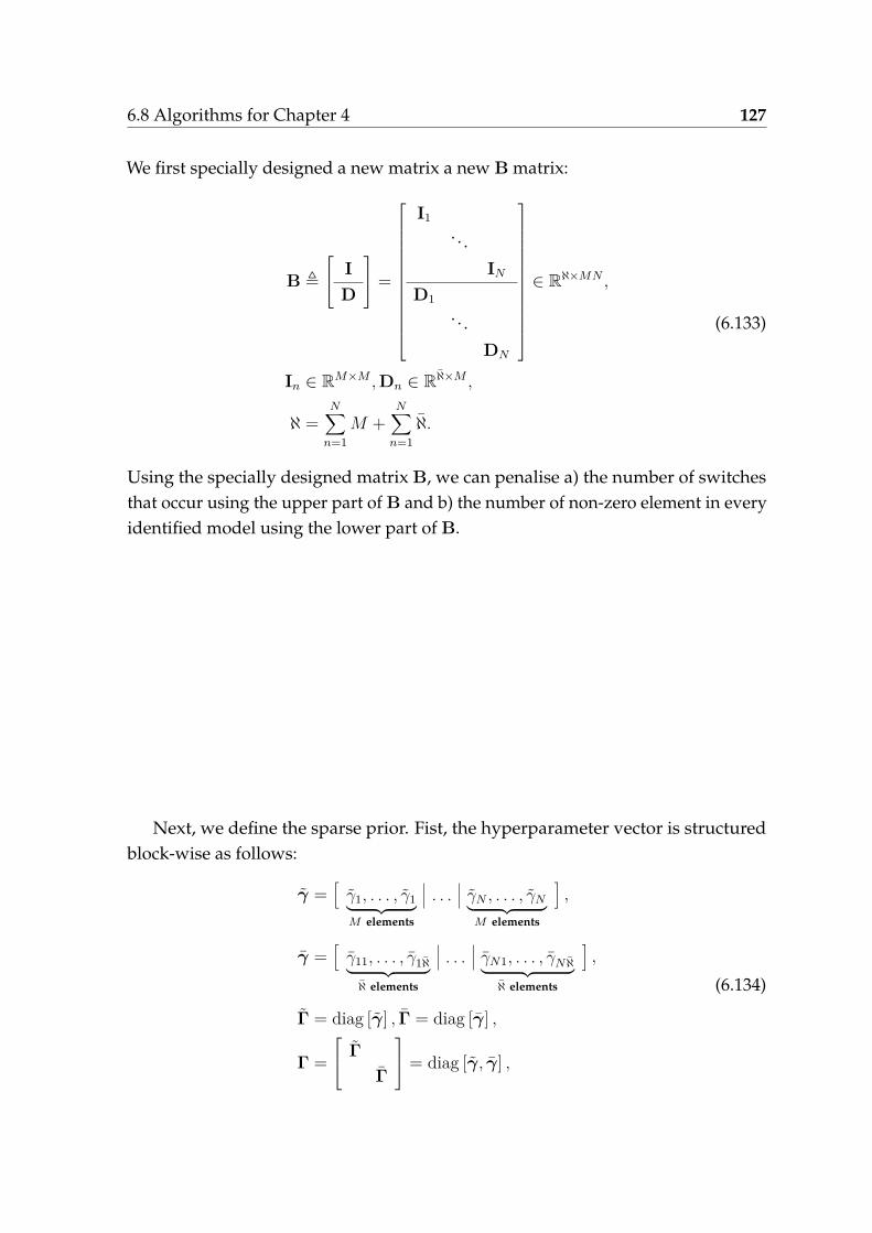
6.8 Algorithms for Chapter 4 127
We first specially designed a new matrix a new B matrix:
B ≜ I
D
=
I1. . .
IN
D1. . .
DN
∈ Rℵ×MN ,
In ∈ RM×M , Dn ∈ Rℵ×M ,
ℵ =N∑
n=1M +
N∑n=1ℵ.
(6.133)
Using the specially designed matrix B, we can penalise a) the number of switchesthat occur using the upper part of B and b) the number of non-zero element in everyidentified model using the lower part of B.
Next, we define the sparse prior. Fist, the hyperparameter vector is structuredblock-wise as follows:
γ =[
γ1, . . . , γ1︸ ︷︷ ︸M elements
. . . γN , . . . , γN︸ ︷︷ ︸M elements
],
γ =[
γ11, . . . , γ1ℵ︸ ︷︷ ︸ℵ elements
. . . γN1, . . . , γN ℵ︸ ︷︷ ︸ℵ elements
],
Γ = diag [γ] , Γ = diag [γ] ,
Γ = Γ
Γ
= diag [γ, γ] ,
(6.134)

128 Algorithms for Likelihood in Gaussian
then get the sparse prior as
p(Bβ) = N (Bβ|0, Γ)φ(Γ)
=N∏
n=1p(βn) ·
N∏n=1
p(Dnβn)
= N (β|0, Γ)φ(Γ) · N (Dβ|0, Γ)φ(Γ)
=N∏
n=1N (βn|0, γnIℵ)φ(γn) ·
N∏n=1N (Dnβn|0, γnIℵ)φ(γn)
=N∏
n=1
M∏i=1N ({In}i,: βn|0, γn)φ(γn) ·
N∏n=1
ℵ∏i=1N ({Dn}i,: βn|0, γn)φ(γn).
(6.135)
6.8.2 Optimisation Algorithm
Optimisation Problem Definition
The optimisation problem is defined exactly the same as (6.13) in Proposition 4.
Convex-Concave Procedure
We first look at the hyperparameter Γ. Since
M∑i=1
(β⊤
n βn
γn
+ αknγn
)≥ 2
∥∥∥∥√Mαkn · βn
∥∥∥∥ℓ2
, (6.136)
the optimal γ can be obtained as:
γk+1n =
∥βn∥ℓ2√Mαk
n
,∀i. (6.137)
Recall the expression for αk in (6.36)
αk ≜∇γv(γ, Π)⊤|γ=γk
=∇γ
(− log |Θ∗|+ log |Γ|+ log |B⊤Γ−1B + X⊤Θ∗X|
)⊤|γ=γk
=− diag{(Γk)−1
}◦ diag
{B(B⊤(Γk)−1B + X⊤Θ∗X)−1B⊤
}◦ diag
{(Γk)−1
}+ diag
{(Γk)−1
},
=[
αk1 · · · αk
N
]

6.8 Algorithms for Chapter 4 129
where Π−1 = Θ = Θ∗. Slightly different from the above expression, αk can bederived in a decomposed way
αk =∇γv(γ, γk, Θ∗)⊤|γ=γk
=∇γ
[log |(Γ)−1 + D⊤(Γk)−1D + X⊤Θ∗X|+ log |Γ|+ log |Γk|
]|γ=γk
= diag{(
(Γk)−1 + D⊤(Γk)−1D + X⊤Θ∗X)−1
}· diag
{−(Γk)−2
}+ diag−1
{Γk}
,
=[
αk11, . . . , αk
1M︸ ︷︷ ︸M elements
. . . αkN1, . . . , αk
NM︸ ︷︷ ︸M elements
].
(6.138)
It is found that αkn is a function of γk
n. Therefore we need to estimate βk+1 first tocalculate γk+1.
We then look at the hyperparameter Γ. Since
β⊤n {Dn}⊤
i,: {Dn}i,: βn
γni
+ αkniγni ≥ 2
∣∣∣∣√αkni · {Dn}i,: βn
∣∣∣∣ (6.139)
the optimal γ can be obtained as
γk+1ni =
| {Dn}i,: βn|√αk
ni
,∀n = 1, . . . , N, i = 1, . . . , ℵ. (6.140)
And αk is defined as
αk =[
αk11, . . . , αk
1ℵ︸ ︷︷ ︸ℵ elements
. . . αkN1, . . . , αk
N ℵ︸ ︷︷ ︸ℵ elements
]. (6.141)
It should be noted that, we can obtain the following analytic form for the negativegradient of v(γ) at γ using basic principles in convex analysis as (using chain rule):
αk =∇γv(γk, γ, Θ∗)⊤|γ=γk
=∇γ
[log |(Γk)−1 + D⊤Γ−1D + X⊤Θ∗X|+ log |Γk|+ log |Γ|
]|γ=γk
= diag{
D((Γk)−1 + D⊤(Γk)−1D + X⊤Θ∗X
)−1D⊤
}· diag
{−(Γk)−2
}+ diag−1
{Γk}
=[
αk11, . . . , αk
1ℵ︸ ︷︷ ︸ℵ elements
. . . αkN1, . . . , αk
N ℵ︸ ︷︷ ︸ℵ elements
].
(6.142)
It is found that αkni is a function of γk
ni. Therefore we need to estimate βk+1n first to
calculate γk+1ni .

130 Algorithms for Likelihood in Gaussian
Two new variables are defined, i.e.,
wkn ≜
√√√√ M∑i=1
αkni, (6.143)
and
wkni ≜
√αk
ni. (6.144)
The pseudo code is summarised in Algorithm 6.
Algorithm 6 Reweighted Fused Group ℓ1 type algorithm for Gaussian likelihood
1: Select the candidate basis functions that will be used to construct the dictionarymatrix described;
2: Initialise wkn = 1, wk
ni = 1, ∀i;3: Fix/given the known inverse covariance matrix Π−1 = Θ = Θ∗;4: Fix λ = 1 and λ = 1 or select λ ∈ R+ and λ ∈ R+ as trail and error which may be
empirically helpful;5: for k = 1, . . . , kmax do6: Solve the following weighted Fused Group Lasso type algorithm
βk+1 = argminβ
(y−Xβ)⊤ Θ∗ (y−Xβ)
+ λN∑
n=1
∥∥∥wkn · βn
∥∥∥ℓ2
+ λN∑
n=1
ℵ∑i=1
∥∥∥wkni · {Dn}i,: βn
∥∥∥ℓ1
; (6.145)
7: γk+1n =
∥βk+1n ∥
ℓ2wk
n, and γk+1 =
[γk+1
1 , . . . , γk+11︸ ︷︷ ︸
M elements
. . . γk+1N , . . . , γk+1
N︸ ︷︷ ︸M elements
];
8: γk+1ni = |{Dn}i,:β
k+1n |
wkni
, ∀n, i, and γk+1 =[
γk+111 , . . . , γk+1
1ℵ︸ ︷︷ ︸ℵ elements
. . . γk+1N1 , . . . , γk+1
N ℵ︸ ︷︷ ︸ℵ elements
];
9: Ck+1 =((Γk+1)−1 + D⊤(Γk+1)−1D + X⊤Θ∗X
)−1;
10: αk+1n = − Ck+1
(γk+1n )2 + 1
γk+1n
;
11: wk+1n =
√M · αk+1
n ;
12: αk+1ni = −{Dn}i,:Ck+1{Dn}⊤
i,:(γk+1
n )2 + 1γk+1
n;
13: wk+1ni =
√αk+1
ni ;14: if a stopping criterion is satisfied then15: Break;16: end if17: end for

Chapter 7
Algorithms for Likelihood inExponential Family

132 Algorithms for Likelihood in Exponential Family
In this Chapter, we go beyond the nonlinear system where the basis functionsare assumed to be “linear in parameters” like Assumption 2. We will considerthe more general model class like Assumption 3. Furthermore, we will cover thedata likelihood beyond Gaussian distribution. Therefore, we move from linearregression with structural sparsity to the more general nonlinear regression withstructural sparsity problems. Similar to Chapter 6, this chapter is organised asfollows. In Section 7.1, we introduce the data likelihood considered in this Chapter,belonging to exponential family. In Section 7.2, the sparse prior and some variationswill be introduced as a controller for the structural sparsity. Next in Section 7.3,the optimisation problem from a Bayesian perspective will be defined. Then inSection 7.5, the general optimisation algorithms are proposed. In the last Section,optimisation algorithms for two special prior will be proposed respectively.
7.1 Likelihood in Exponential Family
Assume the the distribution of data likelihood belongs to exponential family [153,46, 105], i.e.,
p(y|β, θ) = h(β)a(θ) exp(
S∑s=1
ηs(θ) · Ts(β))
= a(θ) exp(
S∑s=1
ηs(θ) · Ts(β) + B(β))
≜ a(θ) exp (−E(β, θ))
(7.1)
where E(∗) is called the energy function.
The exponential families include many of the most commonly used probabilitydistributions. Among many others, the family includes the following: normal,exponential, gamma, chi-squared, beta, Dirichlet, Bernoulli, categorical, Poisson,Wishart, Inverse Wishart. A number of common distributions are exponentialfamilies, but only when certain parameters are fixed and known. For example:binomial (with fixed number of trials), multinomial (with fixed number of trials),negative binomial (with fixed number of failures). Most of the distributions can becovered by exponential family.

7.2 Sparse Prior 133
7.2 Sparse Prior
7.2.1 Generalised Sparse Prior
We still employ the sparse prior in super-Gaussian distribution in Section 6.2 ofChapter 6, i.e.,
p(Bβ) =ℵ∏
i=1N (Bi,:β|0, γi)φ(γi)
= maxγ≻0N (Bβ|0, Γ)φ(γ),
whereγ = [γ1, . . . , γℵ] ∈ Rℵ, Γ = diag [γ] .
In this Section, we vary the structure of B with easy identified name which willbe used throughout the thesis. The “generalised” sparse prior is named after the“generalised lasso” in [190].
BIdentity First, we introduce the simplest case, identity matrix,
B = BIdentity ≜ I =
1
. . .
1
∈ Rℵ×ℵ. (7.2)
Like (4.12) in Section 4.4.2, we introduce BSwitch-I
B = BSwitch-I ≜
D1
. . .
DO
∈ Rℵ×N ,
Do ≜
1 −1
. . . . . .
1 −1
∈ Rℵo×(ℵo+1),
ℵ =O∑
o=1ℵo, N =
O∑o=1
(ℵo + 1), o = 1, . . . , O.
(7.3)

134 Algorithms for Likelihood in Exponential Family
Rather than diagonalise the D matrix, we introduce BSwitch-II
B = BSwitch-II ≜[
D1 . . . DO
]∈ Rℵ×N ,
Do ≜
1 −1
. . . . . .
1 −1
∈ Rℵo×(ℵo+1),
ℵ = ℵo, N =O∑
o=1(ℵo + 1), o = 1, . . . , O.
(7.4)
Like the one introduced in (4.23) for trend filtering, we define BTrend-I
B = BTrend-I ≜
D1
. . .
DO
∈ Rℵ×N ,
Do ≜
1 −2 −1
. . . . . . . . .
1 −2 1
∈ Rℵo×(ℵo+2),
ℵ =O∑
o=1ℵo, N =
O∑o=1
(ℵo + 2), o = 1, . . . , O.
(7.5)
Rather than diagonalise the D matrix, we introduce BTrend-II
B = BTrend-II ≜[
D1 . . . DC
]∈ Rℵ×N ,
Do ≜
1 −2 −1
. . . . . . . . .
1 −2 1
∈ Rℵo×(ℵo+2),
ℵ = ℵo, N =O∑
o=1(ℵo + 2), o = 1, . . . , O.
(7.6)
7.2.2 Group Sparse Prior
In this Section, suppose β is structured block-wise as
β =
β1...
βO
∈ RN (7.7)

7.2 Sparse Prior 135
where βo ∈ RNo and N = ∑Oo=1 No. Furthermore, we introduce the B matrix as
BGroup
B = BGroup ≜
B1
. . .
BO
∈ Rℵ×N ,
Bo ∈ Rℵo×No ,ℵ =O∑
o=1ℵo, N =
O∑o=1
No.
(7.8)
Then we have
Bβ = B
β1...
βO
=
B1β1
...BOβO
=
{B1}1,:β1...
{B1}ℵ1,:β1...
{BO}1,:βO
...{BO}ℵO,:βO
. (7.9)
Next, we define the sparse prior. Fist, the hyperparameter vector is structuredblock-wise as follows:
γ =[
γ1, . . . , γ1︸ ︷︷ ︸ℵ1 elements
. . . γO, . . . , γO︸ ︷︷ ︸ℵO elements
],
Γ = diag [γ] .
(7.10)
and define the sparse prior as
p(Bβ) = N (Bβ|0, Γ)φ(Γ)
=O∏
o=1p(Boβo)
=O∏
o=1N (Boβo|0, γoIℵ)φ(γo)
=O∏
o=1
ℵo∏i=1N ({Bo}i,:βo|0, γo)φ(γo).
(7.11)
The algorithm is introduced later in Section 7.5.1.

136 Algorithms for Likelihood in Exponential Family
7.2.3 Fused Sparse Prior
In this Section, suppose β is structured block-wise as follows:
β =
β1...
βO
=
β1...
βO
where βO ∈ RNo and βO ∈ RNo and N = ∑O
o=1 No = ∑Oo=1 No. It should be noted that
βo may have different dimension with βO, i.e. No = No. Furthermore, we introducethe B matrix as BGroup, where the corresponding B matrix as BFused
B = BFused ≜ B
B
=
B1. . .
BO
B1. . .
BO
∈ Rℵ×N ,
Bo ∈ Rℵo×No , Bo ∈ Rℵo×No ,
ℵ =O∑
o=1ℵo +
O∑o=1ℵo, N =
O∑o=1
No =O∑
o=1No.
(7.12)
Next, we define the sparse prior. First, the hyperparameter vector is structuredblock-wise as follows:
γ =[
γ1, . . . , γ1︸ ︷︷ ︸ℵ1 elements
. . . γO, . . . , γO︸ ︷︷ ︸ℵO elements
],
γ =[
γ11, . . . , γ1ℵ1︸ ︷︷ ︸ℵ1 elements
. . . γO1, . . . , γOℵO︸ ︷︷ ︸ℵO elements
],
Γ = diag [γ] , Γ = diag [γ] ,
Γ = Γ
Γ
= diag [γ, γ] .
(7.13)

7.3 Optimisation Problem Definition 137
Then define the sparse prior as
p(Bβ) = N (Bβ|0, Γ)φ(Γ)= N (Bβ|0, Γ)φ(Γ) · N (Bβ|0, Γ)φ(Γ)
=O∏
o=1p(Boβo) ·
O∏o=1
p(Boβo)
=O∏
o=1N (Boβo|0, γoIℵ)φ(γo) ·
O∏o=1N (Boβo|0, γoIℵ)φ(γo)
=O∏
o=1
ℵo∏i=1N ({Bo}i,:βo|0, γo)φ(γo) ·
O∏o=1
ℵo∏i=1N ({Bo}i,:βo|0, γo)φ(γo).
(7.14)
The algorithm is summarised in Section 7.5.2.
7.3 Optimisation Problem Definition
Once we introduce the likelihood in (7.1) and the variational prior in (6.9), we canget the following approximated optimisation problem jointly on β, γ and Θ.
Proposition 10 Given the likelihood with exponential family distribution p(y|β, θ) =a(θ) exp (−E(β, θ)) as in (7.1) and sparse prior with super Gaussian distribution p(Bβ) =maxγ≻0N (Bβ|0, Γ)φ(γ) as in (6.9), the unknown parameter β, hyperparameter γ, andparameter of the family θ can be approximately obtained by solving the following optimisationproblem
minβ,γ,θL(β, γ, θ) (7.15)
with
L(β, γ, θ) = β⊤H(β∗, θ)β + 2β⊤ [g(β∗, θ)−H(β∗, θ)β∗] + β⊤B⊤Γ−1Bβ
+ log |Γ|+ log |H(β∗, θ) + B⊤Γ−1B| − 2 log a(θ) · b(β∗, θ)− 2ℵ∑
i=1log φ(γi) (7.16)
where β∗ is arbitrary, and
g(β∗, θ) ≜ ∇E(β, θ)|β∗ , H(β∗, θ) ≜ ∇∇E(β, θ)|β∗ .
andb(β∗, θ) ≜ exp
{−(1
2β∗⊤H(β∗, θ)β∗ − β∗⊤g(β∗, θ) + E(β∗, θ))}
.

138 Algorithms for Likelihood in Exponential Family
Proof Given the likelihood with exponential family distribution
p(y|β, θ) = a(θ) exp (−E(β, θ))
as in (7.1) and sparse prior with super Gaussian distribution
p(Bβ) = maxγ≻0N (Bβ|0, Γ)φ(γ)
as in (6.9), we go straightly into the marginal likelihood
∫p(y|β, θ)N (Bβ|0, Γ)
ℵ∏i=1
φ(γi)dβ
=a(θ)∫
exp{−E(β, θ)}N (Bβ|0, Γ)ℵ∏
i=1φ(γi)dβ
=a(θ)∫
exp(
S∑s=1
ηs(θ) · Ts(β) + B(β))N (Bβ|0, Γ)
ℵ∏i=1
φ(γi)dβ.
(7.17)
Typically, this integral is intractable or has no analytical solution.
We first fix θ, the parameter of the family. For example, the mean and covariance can befixed if the family is Gaussian. Performing a Taylor series expansion around some point β∗,E(β, θ) can be approximated as
E(β, θ) ≈ E(β∗, θ) + (β − β∗)⊤g(β∗, θ) + 12(β − β∗)⊤H(β∗, θ)(β − β∗) (7.18)
where g(·) is the gradient and H(·) is the Hessian of the energy function E
g(β∗, θ) ≜ ∇E(β, θ)|β∗ = −(
S∑s=1
ηs(θ) · ∇Ts(β)|β∗ +∇B(β)|β∗
), (7.19a)
H(β∗, θ) ≜ ∇∇E(β, θ)|β∗ = −(
S∑s=1
ηs(θ) · ∇∇Ts(β)|β∗ +∇∇B(β)|β∗
). (7.19b)
To derive the cost function in (7.16), we introduce the posterior mean and covariance
mβ = Σβ · [g(β∗, θ) + H(β∗, θ)β∗] , (7.20a)
Σβ =[H(β∗, θ) + B⊤Γ−1B
]−1. (7.20b)

7.3 Optimisation Problem Definition 139
Then define the following quantities
b(β∗, θ) ≜ exp{−(1
2β∗⊤H(β∗, θ)β∗ − β∗⊤g(β∗, θ) + E(β∗, θ))}
, (7.21a)
c(β∗, θ) ≜ exp{1
2 g(β∗, θ)⊤H(β∗, θ)g(β∗, θ)}
, (7.21b)
d(β∗, θ) ≜√|H(β∗, θ)|, (7.21c)
g(β∗, θ) ≜ g(β∗, θ)−H(β∗, θ)β∗. (7.21d)
Now the approximated likelihood p(y|β, θ) is a exponential of quadratic, then Gaussian,
p(y|β, θ)=a(θ) · exp{−E(β, θ)}
≈a(θ) · exp{−(1
2(β − β∗)⊤H(β∗, θ)(β − β∗) + (β − β∗)⊤g(β∗, θ) + E(β∗, θ))}
=a(θ) · exp{−(1
2β⊤H(β∗, θ)β + β⊤ [g(β∗, θ)−H(β∗, θ)β∗])}
· exp{−(1
2β∗⊤H(β∗, θ)β∗ − β∗⊤g(β∗, θ) + E(β∗, θ))}
=a(θ) · b(β∗, θ) · exp{−(1
2β⊤H(β∗, θ)β + β⊤g(β∗, θ))}
· exp{1
2 g(β∗, θ)⊤H(β∗, θ)g(β∗, θ)− 12 g(β∗, θ)⊤H(β∗, θ)g(β∗, θ)
}=a(θ) · b(β∗, θ) · c(β∗, θ)
· exp{−(1
2β⊤H(β∗, θ)β + β⊤g(β∗, θ) + 12 g(β∗, θ)⊤H(β∗, θ)g(β∗, θ)
)}=(2π)M/2a(θ)b(β∗, θ)c(β∗, θ)d(β∗, θ) · N (β|β∗, H−1(β∗, θ))≜A(β∗, θ) · N (β|β∗, H−1(β∗, θ)),
(7.22)where
A(β∗, θ) = (2π)M/2a(θ)b(β∗, θ)c(β∗, θ)d(β∗, θ),β∗ = −H−1(β∗, θ)g(β∗, θ) = β∗ −H−1(β∗, θ)g(β∗, θ).

140 Algorithms for Likelihood in Exponential Family
We can write the approximate marginal likelihood as
A(β∗, θ)∫N (β|β∗, H−1(β∗, θ)) · N (Bβ|0, Γ)
ℵ∏i=1
φ(γi)dβ
=a(θ) · b(β∗, θ) ·∫
exp{−(1
2β⊤H(β∗, θ)β + β⊤g(β∗, θ))}N (Bβ|0, Γ)
ℵ∏i=1
φ(γi)dβ
=a(θ) · b(β∗, θ)(2π)ℵ/2 |Γ|1/2
∫exp{−E(β, θ)}dβ
ℵ∏i=1
φ(γi),
(7.23)where
E(β) = 12β⊤H(β∗, θ)β + β⊤g(β∗, θ) + 1
2β⊤B⊤Γ−1Bβ. (7.24)
Equivalently, we get
E(β) = 12(β −mβ)⊤Σ−1
β (β −mβ) + E(y), (7.25)
where mβ and Σβ are given in (7.20). From (7.20a) and (7.20b), the data-dependent termcan be re-expressed as
E(y) =12m⊤
β H(β∗, θ)mβ + m⊤β g(β∗, θ) + 1
2m⊤β B⊤Γ−1Bmβ
= minβ
[12β⊤H(β∗, θ)β + β⊤g(β∗, θ) + 1
2β⊤B⊤Γ−1Bβ]
= minβ
[12β⊤H(β∗, θ)β + β⊤ (g(β∗, θ)−H(β∗, θ)β∗) + 1
2β⊤B⊤Γ−1Bβ]
.
(7.26)
Using (7.25), we can evaluate the integral in (7.23) to obtain
∫exp
{−E(β)
}dβ = exp
{−E(y)
}(2π)ℵ|Σβ|1/2. (7.27)
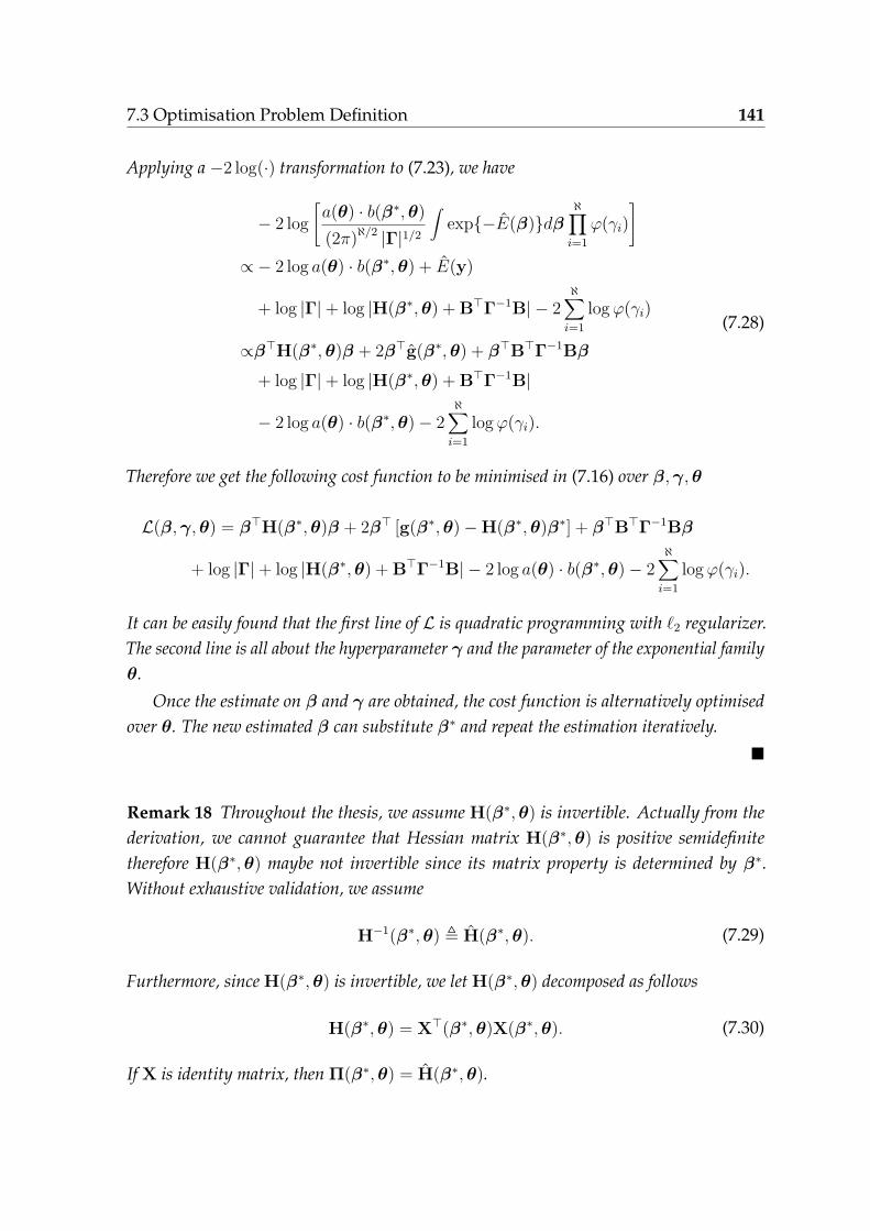
7.3 Optimisation Problem Definition 141
Applying a −2 log(·) transformation to (7.23), we have
− 2 log[
a(θ) · b(β∗, θ)(2π)ℵ/2 |Γ|1/2
∫exp{−E(β)}dβ
ℵ∏i=1
φ(γi)]
∝− 2 log a(θ) · b(β∗, θ) + E(y)
+ log |Γ|+ log |H(β∗, θ) + B⊤Γ−1B| − 2ℵ∑
i=1log φ(γi)
∝β⊤H(β∗, θ)β + 2β⊤g(β∗, θ) + β⊤B⊤Γ−1Bβ
+ log |Γ|+ log |H(β∗, θ) + B⊤Γ−1B|
− 2 log a(θ) · b(β∗, θ)− 2ℵ∑
i=1log φ(γi).
(7.28)
Therefore we get the following cost function to be minimised in (7.16) over β, γ, θ
L(β, γ, θ) = β⊤H(β∗, θ)β + 2β⊤ [g(β∗, θ)−H(β∗, θ)β∗] + β⊤B⊤Γ−1Bβ
+ log |Γ|+ log |H(β∗, θ) + B⊤Γ−1B| − 2 log a(θ) · b(β∗, θ)− 2ℵ∑
i=1log φ(γi).
It can be easily found that the first line of L is quadratic programming with ℓ2 regularizer.The second line is all about the hyperparameter γ and the parameter of the exponential familyθ.
Once the estimate on β and γ are obtained, the cost function is alternatively optimisedover θ. The new estimated β can substitute β∗ and repeat the estimation iteratively.
■
Remark 18 Throughout the thesis, we assume H(β∗, θ) is invertible. Actually from thederivation, we cannot guarantee that Hessian matrix H(β∗, θ) is positive semidefinitetherefore H(β∗, θ) maybe not invertible since its matrix property is determined by β∗.Without exhaustive validation, we assume
H−1(β∗, θ) ≜ H(β∗, θ). (7.29)
Furthermore, since H(β∗, θ) is invertible, we let H(β∗, θ) decomposed as follows
H(β∗, θ) = X⊤(β∗, θ)X(β∗, θ). (7.30)
If X is identity matrix, then Π(β∗, θ) = H(β∗, θ).

142 Algorithms for Likelihood in Exponential Family
We note that in (7.19), β∗ may not be the mode (i.e., the lowest energy state),which means the gradient term g may not be zero. Therefore the selection of β∗
1
remains to be problematic. We give the following Corollary to address this issue,which is more general.
Corollary 2 Suppose
β∗ = argminβ
E(β, θ) + β⊤B⊤Γ−1Bβ, (7.31)
we define a new cost function
L(β, γ, θ) ≜ E(β, θ) + β⊤B⊤Γ−1Bβ
+ log |Γ|+ log |H(β∗, θ) + B⊤Γ−1B| − 2 log a(θ) · b(β∗, θ)− 2ℵ∑
i=1log φ(γi). (7.32)
Instead of minimising L(β, γ, θ), we can solve the following optimisation problem to getβ, γ, θ
minβ,γ,θL(β, γ, θ).
Proof Since the likelihood is
p(y|β, θ) = a(θ) · exp{−E(β, θ)},
thenmin
βE(β, θ) + β⊤B⊤Γ−1Bβ
is exactly the regularised maximum likelihood estimation with ℓ2 type regulariser.We look at the first part of L(β, γ, θ) in (7.16), and define them as
L0(β, γ, θ) ≜ β⊤H(β∗, θ)β + 2β⊤ [g(β∗, θ)−H(β∗, θ)β∗] + β⊤B⊤Γ−1Bβ,
then
minβL0(β, γ, θ)
= minβ
12(β − β∗)⊤H(β∗, θ)(β − β∗) + (β − β∗)⊤g(β∗, θ) + E(β∗, θ) + β⊤B⊤Γ−1Bβ
≈minβ
E(β, θ) + β⊤B⊤Γ−1Bβ
(7.33)

7.4 Optimisation Algorithm 143
where, given (7.19),g(β, θ) = ∇E(β, θ)
H(β, θ) = ∇∇E(β, θ).(7.34)
Such quadratic approximation to E(β, θ) + β⊤B⊤Γ−1Bβ is actually the same as theapproximation procedure in Trust-Region Methods where a region is defined around thecurrent iterate within which they trust the model to be an adequate representation of theobjective function [219, pp.65].
Similar to [219, eq.(4.3)], to obtain each step, we seek a solution of the subproblem atiteration k
minβ
Ek(β, θ) + β⊤B⊤Γ−1Bβ
= minβ
12(β − βk)⊤H(βk, θ)(β − βk) + (β − βk)⊤g(βk, θ) + β⊤B⊤Γ−1Bβ
(7.35)
Supposeβ∗ = argmin
βE(β, θ) + β⊤B⊤Γ−1Bβ,
then inject β∗ into minβ,γ,θ L(β, γ, θ), we can optimise (7.32) instead of (7.16), i.e.,minβ,γ,θ L(β, γ, θ).
■
7.4 Optimisation Algorithm
In this Section, we propose iterative optimisation algorithms to estimate β, γ and θ
alternatively.
7.4.1 Optimisation for unknown parameter β and hyperparameterγ
Convex-concave procedure
We first target for the estimation of unknown parameter β and hyperparameter γ.We first initialise θ to some reasonable value or have already had a good estimateof θ, denoted as θ∗. Then H(β∗, θ∗) is a known symmetric matrix, assuming tobe positive semidefinite. In the sequel, we show that the stated program can beformulated as a convex-concave procedure (CCCP) for β and γ.

144 Algorithms for Likelihood in Exponential Family
Proposition 11 The following programme
minβ,γL(β, γ)
with the cost function defined as
L(β, γ) ≜ β⊤H(β∗, θ∗)β + 2β⊤ [g(β∗, θ∗)−H(β∗, θ∗)β∗] + β⊤B⊤Γ−1Bβ
+ log |Γ|+ log |B⊤Γ−1B + H(β∗, θ∗)| (7.36)
can be formulated as a convex-concave procedure (CCCP), where β∗ and θ∗ can be arbitraryreal vector.
Proof Fact on convexity: the function
u (β, Γ) =β⊤H(β∗, θ∗)β + 2β⊤ [g(β∗, θ∗)−H(β∗, θ∗)β∗] + β⊤B⊤Γ−1Bβ
∝(β − β∗)⊤H(β∗, θ∗)(β − β∗) + 2β⊤g(β∗, θ∗) + β⊤B⊤Γ−1Bβ(7.37)
is convex jointly in β, Γ due to the fact that f(x, Y ) = x⊤Y−1x is jointly convex in x, Y(see, [28, p.76]). Hence u as a sum of convex functions is convex.
Fact on concavity: the function
v(Γ) = log |Γ|+ log |B⊤Γ−1B + H(β∗, θ∗)| (7.38)
is jointly concave in Γ, Π. We exploit the properties of the determinant of a matrix
|A22||A11 − A12A−122 A21| =
∣∣∣∣∣∣A11 A12
A21 A22
∣∣∣∣∣∣ = |A11||A22 − A21A−111 A12|.
Then we have
v(Γ) = log |Γ|+ log |B⊤Γ−1B + H(β∗, θ∗)|= log
(|Γ||B⊤Γ−1B + H(β∗, θ∗)|
)= log
∣∣∣∣∣∣H(β∗, θ∗) B⊤
B −Γ
∣∣∣∣∣∣= log
∣∣∣Γ + BH−1(β∗, θ∗)B⊤∣∣∣+ log |H(β∗, θ∗)|
(7.39)
which is a log-determinant of an affine function of semidefinite matrices Π, Γ and henceconcave.

7.4 Optimisation Algorithm 145
Therefore, we can derive the iterative algorithm solving the CCCP. We have the followingiterative convex optimisation program by calculating the gradient of concave part.
βk+1 = argminβ
u(β, γk, H(β∗, θ∗)), (7.40)
γk+1 = argminγ⪰0
u(βk, γ, H(β∗, θ∗)) +∇γv(γk, H(β∗, θ∗))⊤γ. (7.41)
■
Remark 19 Remark on the log of potential function in Proposition 11. Refer to the samecontents in Remark 13.
Derivation of iterative reweighted ℓ1 algorithm
Using basic principles in convex analysis, we then obtain the following analytic formfor the negative gradient of v(γ) at γ is (using chain rule):
αk ≜∇γv (γ, H(β∗, θ∗))⊤ |γ=γk
=∇γ
(log |B⊤Γ−1B + H(β∗, θ∗)|+ log |Γ|
)⊤|γ=γk
=− diag{(Γk)−1
}◦ diag
{B(B⊤(Γk)−1B + H(β∗, θ∗)
)−1B⊤
}◦ diag
{(Γk)−1
}+ diag
{(Γk)−1
}=[
αk1 · · · αk
N
](7.42)
where ◦ denote the Hadamard product operation (entrywise multiplication) anddiag denote the operation to get diagonal elements of matrix. Then equivalently, wehave
αki = −
Bi,:(B⊤(Γk)−1B + H(β∗, θ∗))−1B⊤i,:
(γki )2 + 1
γki
. (7.43)
Therefore, the iterative procedures (7.40) and (7.41) for βk+1 and γk+1 can be formu-lated as[
βk+1, γk+1]
= argminγ⪰0,β
(β − β∗)⊤H(β∗, θ∗)(β − β∗) + 2β⊤g(β∗, θ∗) +ℵ∑
i=1
(β⊤B⊤
i,:Bi,:β
γi
+ αki γi
)
= argminβ
β⊤H(β∗, θ∗)β + 2β⊤ (g(β∗, θ∗)−H(β∗, θ∗)β∗) +ℵ∑
i=1
(β⊤B⊤
i,:Bi,:β
γi
+ αki γi
).
(7.44)

146 Algorithms for Likelihood in Exponential Family
Or in the compact form
[βk+1, γk+1
]= argmin
ββ⊤H(β∗, θ∗)β + 2β⊤ (g(β∗, θ∗)−H(β∗, θ∗)β∗)
+ β⊤B⊤Γ−1B +ℵ∑
i=1αk
i γi.(7.45)
Sinceβ⊤B⊤
i,:Bi,:β
γi
+ αki γi ≥ 2
∣∣∣∣√αki ·Bi,:β
∣∣∣∣ ,the optimal γ can be obtained as:
γi = |Bi,:β|√αk
i
, ∀i. (7.46)
From (7.42), it is found that αki is a function of γk
i . Therefore we need to estimateβk+1 first to calculate γk+1. If we define
wki ≜
√αk
i =
√√√√−Bi,:(B⊤(Γk)−1B + H(βk, θ∗))−1B⊤i,:
(γki )2 + 1
γki
. (7.47)
βk+1 can be obtained as follows
βk+1 = argminβ
12β⊤H(β∗, θ∗)β + β⊤ (g(β∗, θ∗)−H(β∗, θ∗)β∗) +
ℵ∑i=1∥wk
i ·Bi,:β∥ℓ1 .
(7.48)We can then inject this into (7.46), which yields
γk+1i = |Bi,:β
k+1|wk
i
,∀i. (7.49)
As we found in the expression for αi in (7.43), αki is function of γk, therefore γk+1
is function of γk and βk+1. We notice that the update for βk+1 is to use the lassoor ℓ1-regularised regression type optimisation. The pseudo code is summarised inAlgorithm 7.

7.4 Optimisation Algorithm 147
Algorithm 7 Reweighted ℓ1 type algorithm for likelihood in exponential family ofdistributions
1: Symbolic cache likelihood, gradient and Hessian expressions
p(y|β, θ) = a(θ) · exp{−E(β, θ)}; g(β, θ) = ∇E(β, θ)|; H(β, θ) = ∇∇E(β, θ);
2: Initialise the unknown w1 as a unit vector;3: Fix/given the known parameter of the exponential family θ = θ∗;4: Fix λ = 1 or select λ ∈ R+ as trail and error which may be empirically helpful;5: for k = 1, . . . , kmax do6:
βk+1 = argminβ
E(β, θ∗) + λℵ∑
i=1∥wk
i ·Bi,:β∥ℓ1 ; (7.50)
7: γk+1i =
∣∣∣∣Bi,:βk+1
wki
∣∣∣∣;8: Ck+1 =
(B⊤(Γk+1)−1B + H(βk+1, θ∗)
)−1;
9: αik+1 = −Bi,:Ck+1B⊤
i,:(γk+1
i )2 + 1γk+1
i
;
10: wik+1 =
√αi
k+1;11: if a stopping criterion is satisfied then12: Break.13: end if14: end for

148 Algorithms for Likelihood in Exponential Family
Derivation of iterative reweighted ℓ2 algorithm
In (7.44), instead of formulating a convex program for β and γ jointly, they areoptimised respectively.
βk+1 = argminβ
(β − β∗)⊤H(β∗, θ∗)(β − β∗) + 2β⊤g(β∗, θ∗) +ℵ∑
i=1
∥∥∥∥∥∥Bi,:β√γk
i
∥∥∥∥∥∥2
ℓ2
,
= argminβ
12β⊤H(β∗, θ∗)β + β⊤ (g(β∗, θ∗)−H(β∗, θ∗)β∗) + 1
2β⊤B⊤(Γk)−1Bβ
= argminβ
E(β, θ∗) + 12β⊤B⊤(Γk)−1Bβ, (7.51)
γk+1i = argmin
γi≥0
(βk+1)⊤B⊤i,:Bi,:β
k+1
γi
+ αki γi,∀i. (7.52)
Once βk+1 is obtained, γk+1 has a closed form solution to (7.52), i.e.,
γk+1i =
√√√√(βk+1)⊤B⊤i,:Bi,:βk+1
αki
,
where αki is the same as (7.43)
αki = −
Bi,:(B⊤(Γk)−1B + H(βk+1, θ∗))−1B⊤i,:
(γki )2 + 1
γki
.
But unlike (7.47), wki is defined as
wki ≜ 1√
γki
.
The pseudo code is summarised in Algorithm 8.

7.4 Optimisation Algorithm 149
Algorithm 8 Reweighted ℓ2 type algorithm for likelihood in exponential family ofdistributions
1: Symbolic cache likelihood, gradient and Hessian expressions
p(y|β, θ) = a(θ) · exp{−E(β, θ)}; g(β, θ) = ∇E(β, θ); H(β, θ) = ∇∇E(β, θ);
2: Initialise the unknown hyperparameter γ1 as a unit vector;3: Fix/given the known parameter of the exponential family θ = θ∗;4: Initialise w1
i = 1, ∀i;5: Fix λ = 1 or select λ ∈ R+ as trail and error which may be empirically helpful;6: for k = 1, . . . , kmax do7:
βk+1 = argminβ
E(β, θ∗) + λ
2 β⊤B⊤(Γk)−1Bβ
= argminβ
E(β, θ∗) + λ
2
ℵ∑i=1∥wk
i ·Bi,:β∥2ℓ2 ;
(7.53)
8: Ck =(B⊤(Γk)−1B + H(βk+1, θ∗)
)−1;
9: αk+1i = −Bi,:CkB⊤
i,:(γk
i )2 + 1γk
i;
10: γk+1i = |Bi,:βk+1|√
αk+1i
;
11: wk+1i = 1√
γk+1i
;
12: if a stopping criterion is satisfied then13: Break.14: end if15: end for
7.4.2 Optimisation for the parameter of the exponential family θ
Once β and γ are given or estimated to be β∗ and γ∗, θ will be estimated, the costfunction is
L(β∗, γ∗, θ) = (β∗)⊤H(β∗, θ)(β∗)+2(β∗)⊤ [g(β∗, θ)−H(β∗, θ)β∗]+(β∗)⊤B⊤Γ∗−1Bβ∗
+ log |Γ∗|+ log |H(β∗, θ) + B⊤(Γ∗)−1B| − 2 log a(θ) · b(β∗, θ)− 2ℵ∑
i=1log φ(γi).
By dropping the constant, the estimate θ∗ can be obtained by minimising the newcost function over θ
θ∗ = argminθL(β∗, γ∗, θ) (7.54)

150 Algorithms for Likelihood in Exponential Family
where
L(β∗, γ∗, θ) = β∗⊤ [2g(β∗, θ)−H(β∗, θ)β∗]+ log |H(β∗, θ) + B⊤(Γ∗)−1B| − 2 log a(θ) · b(β∗, θ).
If the likelihood is Gaussian distributed, an easy recognised algorithm can be foundin Section 6.5.3.
Inspired by the implementation of Generalised Method of Moment (GMM)[76, 77], a Nobel Prize in Economics winning work by Lars Hansen, we propose twoways to optimise for θ.
The first one is inspired by two-step feasible GMM, where after the find estima-tion of β and γ, i.e., at the iteration k = kend of the CCCP (7.40) and (7.41)
βk+1 = argminβ
u(β, γk, H(β∗, θ∗)),
γk+1 = argminγ⪰0
u(βk, γ, H(β∗, θ∗)) +∇γv(γk, H(β∗, θ∗))⊤γ,
we haveθ∗ = argmin
θL(βkend , γkend , θ). (7.55)
The second one is inspired by iterated GMM, where at each iteration k of theCCCP (7.40) and (7.41), we perform
βk+1 = argminβ
u(β, γk, H(β∗, θ∗)),
γk+1 = argminγ⪰0
u(βk, γ, H(β∗, θ∗)) +∇γv(γk, H(β∗, θ∗))⊤γ,
θk+1 = argminθL(βk+1, γk+1, θ).
(7.56)
7.4.3 Implementations
Iterative Solvers
One of the main step in Algorithm 7 and 8 are the penalised MAP optimisation,i.e., reweighted ℓ1 regression (7.50) and reweighted ℓ2 regression (7.53). This is moregeneral yet able to build upon the Alternating Direction Method of Multipliers (ADMM)method [27]. When E is smooth, general iterative methods can be used to carryout the β-minimization step. Of particular interest are methods that only requirethe ability to compute ∇βE for a given β. Such methods can scale to relatively

7.4 Optimisation Algorithm 151
large problems. Examples include the standard gradient method, the (nonlinear)conjugate gradient method, and the limited-memory Broyden-Fletcher-Goldfarb-Shanno (L-BFGS) algorithm [29, 116]; see [219] for further details.
In this Thesis, we will derive corresponding ADMM algorithm for our methodwhich we use mostly in our experiments. Empirical study shows that ADMMscheme is superior in the penalised MAP optimisation problem, both in convergencespeed and solution consistency.
Short-Cut to Computation of the Updated Weight w
The other main step in Algorithm 7 and 8 is the computation to invert the covariancematrix C =
(B⊤Γ−1B + H(β, θ∗)
)−1which typically requires O(N3) computations
andO(N2) memory. We next show that the computation of inverting a matrix can bea by-product of the iterative solvers, namely, Quasi-Newton method such as L-BFGS.Unfortunately, this only applies to reweighted ℓ2 regression (7.53), but not reweighted ℓ1
regression (7.50) yet.
In (7.53) of Algorithm 8, the following minimisation problem is typically solvedby iterative solvers.
βk+1 = argminβ
E(β, θ∗) + 12β⊤B⊤(Γk)−1Bβ.
We denotefk(β) ≜ E(β, θ∗) + 1
2β⊤B⊤(Γk)−1Bβ. (7.57)
And we assume min fk(β) is solved by Newton method where the gradient andHessian information of fk(β) is needed. Typically, the symbolic expression ofgradient ∂fk(β)
∂βand Hessian ∂2fk(β)
∂β∂β⊤ will be cached at the beginning.
It should be noted that H(β) may not be unnecessary if Quasi-Newton methodmethod is employed since the Hessian information can be evaluated/approximatedby the gradient. We change the iteration index k (see the 4th line of Algorithm 8) asepoch, while the iteration index is denoted as τ for solving (7.53) by using iterative
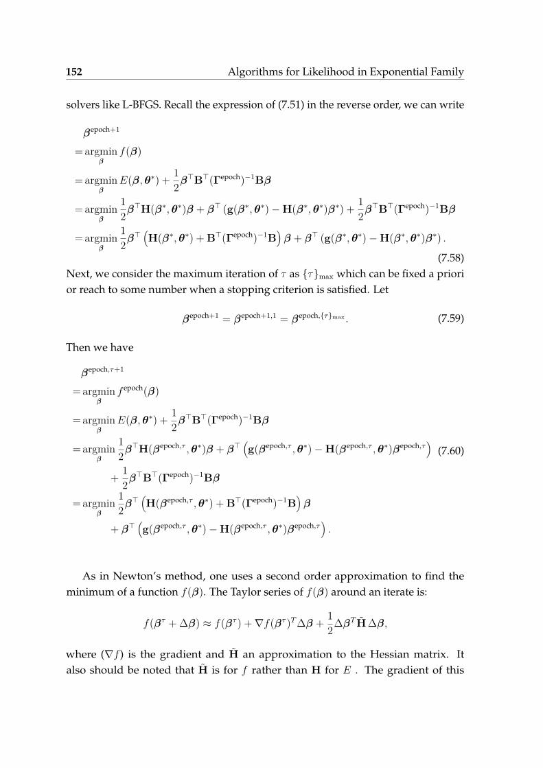
152 Algorithms for Likelihood in Exponential Family
solvers like L-BFGS. Recall the expression of (7.51) in the reverse order, we can write
βepoch+1
= argminβ
f(β)
= argminβ
E(β, θ∗) + 12β⊤B⊤(Γepoch)−1Bβ
= argminβ
12β⊤H(β∗, θ∗)β + β⊤ (g(β∗, θ∗)−H(β∗, θ∗)β∗) + 1
2β⊤B⊤(Γepoch)−1Bβ
= argminβ
12β⊤
(H(β∗, θ∗) + B⊤(Γepoch)−1B
)β + β⊤ (g(β∗, θ∗)−H(β∗, θ∗)β∗) .
(7.58)Next, we consider the maximum iteration of τ as {τ}max which can be fixed a priorior reach to some number when a stopping criterion is satisfied. Let
βepoch+1 = βepoch+1,1 = βepoch,{τ}max . (7.59)
Then we have
βepoch,τ+1
= argminβ
f epoch(β)
= argminβ
E(β, θ∗) + 12β⊤B⊤(Γepoch)−1Bβ
= argminβ
12β⊤H(βepoch,τ , θ∗)β + β⊤
(g(βepoch,τ , θ∗)−H(βepoch,τ , θ∗)βepoch,τ
)+ 1
2β⊤B⊤(Γepoch)−1Bβ
= argminβ
12β⊤
(H(βepoch,τ , θ∗) + B⊤(Γepoch)−1B
)β
+ β⊤(g(βepoch,τ , θ∗)−H(βepoch,τ , θ∗)βepoch,τ
).
(7.60)
As in Newton’s method, one uses a second order approximation to find theminimum of a function f(β). The Taylor series of f(β) around an iterate is:
f(βτ + ∆β) ≈ f(βτ ) +∇f(βτ )T ∆β + 12∆βT H ∆β,
where (∇f ) is the gradient and H an approximation to the Hessian matrix. Italso should be noted that H is for f rather than H for E . The gradient of this

7.4 Optimisation Algorithm 153
approximation (with respect to ∆β) is
∇f(βτ + ∆β) ≈ ∇f(βτ ) + H ∆β
and setting this gradient to zero (which is the objective of optimisation) provides theNewton step:
∆β = −H−1∇f(βτ ),
The Hessian approximation H is chosen to satisfy
∇f(βτ + ∆β) = ∇f(βτ ) + H ∆β,
which is called the “secant equation” (the Taylor series of the gradient itself). Inmore than one dimension H is underdetermined. In one dimension, solving forH and applying the Newton’s step with the updated value is equivalent to thesecant method. The various quasi-Newton methods differ in their choice of thesolution to the secant equation (in one dimension, all the variants are equivalent).Most methods (but with exceptions, such as Broyden’s method) seek a symmetricsolution (H⊤ = H); furthermore, the variants listed below can be motivated byfinding an update Hτ+1 that is as close as possible to Hτ in some norm; that is,Hτ+1 = argminH∥H− Hτ∥V where V is some positive definite matrix that definesthe norm. An approximate initial value of H0 = I ∗ β is often sufficient to achieverapid convergence. Note that H0 should be positive definite. The unknown βτ
is updated applying the Newton’s step calculated using the current approximateHessian matrix Hτ
• ∆βτ = −ατ (Hτ )−1∇f(βτ ), with α chosen to satisfy the Wolfe conditions;
• βτ+1 = βτ + ∆βτ ;
• The gradient computed at the new point ∇f(βτ+1), and
yτ = ∇f(βτ+1)−∇f(βτ ),

154 Algorithms for Likelihood in Exponential Family
is used to update the approximate Hessian Hτ+1, or directly its inverse (Hτ+1)−1
using the Sherman-Morrison formula. For example, using L-BFGS,
Hτ+1 = Hτ + yτ (yτ )⊤
(yτ )⊤∆βτ− Hτ ∆βτ (Hτ ∆βτ )⊤
∆(βτ )⊤Hτ ∆βτ, (7.61a)
(Hτ+1)−1 =(
I− ∆βτ (yτ )⊤
(yτ )⊤∆βτ
)Hτ
(I− yτ ∆(βτ )⊤
(yτ )⊤∆βτ
)+ ∆βτ ∆(βτ )⊤
(yτ )⊤ ∆βτ; (7.61b)
• A key property of the BFGS and DFP updates is that if Hτ is positive definiteand ατ is chosen to satisfy the Wolfe conditions then Hτ+1 is also positivedefinite.
In Algorithm 9, we modify Algorithm 8 with Quasi-Newton method solvingthe minimisation problem (7.53). It should be noted that, if L-BFGS algorithm isemployed, the Hessian matrix needs not to be cached a priori but approximatedby gradient, i.e., approximating Hτ+1 or directly (Hτ+1)−1 by ∇f(βepoch,τ+1) and∇f(βepoch,τ ).
Semidefinite Programming for Arbitrary Γ
To this end, the covariance matrix for the super Gaussian distribution Γ, i.e., thehyperparameter, is diagonal. The underlying implication of “diagonal” is the inde-pendence of γi therefore Bi,:β are independent with each other, ∀i. In other words,all the parameters of a model are irrelevant. Apparently, it should be careful tomake such assumption. For example, in financial models, some parameters areco-moving together; in gene networks, some parameters are changing in response tocertain common external perturbation. In this Section, we will show that the neatand simple form with ℓ1− or ℓ2− regularisation disappears when the covariancematrix Γ is not diagonal, yet semidefinite positive, as an illustration, Γ may look like γ1 γ1γ2
γ1γ2 γ2
.
We first vectorise all the parameters γi into a single vector γ. From (7.30) inRemark 18, we know
H(β∗, θ) = X⊤(β∗, θ)X(β∗, θ).

7.4 Optimisation Algorithm 155
Algorithm 9 Algorithm 8 with Quasi-Newton Update
1: Cache symbolically the likelihood, loss function and its gradient over β
Likelihood: p(y|β, θ) = a(θ) · exp{−E(β, θ)}Loss function: f(β, γ, θ) = E(β, θ) + λβ⊤B⊤Γ−1Bβ
Gradient function: g(β, γ, θ) = ∇βf(β, γ, θ)
where we fix λ = 1 or select λ ∈ R+ as trail and error which may be empiricallyhelpful;
2: Initialise the unknown hyperparameter γ, i.e., γ1, as an arbitrary positive vectorsuch as unit vector;
3: Initialise the unknown parameter β, i.e., β1,1, as an arbitrary real vector such aszero vector;
4: Fix/given the known parameter of the exponential family θ = θ∗;5: Initialise the Hessian matrix H1,1 as an arbitrary positive definite matrix such as
identity or be calculated explicitly with∇∇βf(β, γ, θ) given β1,1 and θ∗;6: for epoch = 1, . . . , epochmax do7: for τ = 1, . . . , τmax do8: Choose αepoch,τ for the next step to via line search under Wolfe conditions;9: ∆βepoch,τ = −αepoch,τ (Hepoch,τ )−1g(βepoch,τ , γepoch, θ∗);
10: βepoch,τ+1 = βepoch,τ + ∆βepoch,τ ;11: Compute the gradient at the new point g(βepoch,τ+1, γepoch, θ∗);12: yepoch,τ = g(βepoch,τ+1, γepoch, θ∗)− g(βepoch,τ , γepoch, θ∗);13: Approximate Hepoch,τ+1 using yepoch,τ , ∆βepoch,τ , Hepoch,τ like (7.61a);14: Approximate (Hepoch,τ+1)−1 using yepoch,τ , ∆βepoch,τ , Hepoch,τ like (7.61b);15: end for16: Cepoch =
(H(βepoch,τmax , θ∗)
)−1;
17: αepoch+1i = −Bi,:CepochB⊤
i,:
(γepochi )2 + 1
γepochi
;
18: βepoch+1 = βepoch,τmax ;
19: γepoch+1i = |Bi,:βepoch+1|√
αepoch+1i
, Γkepoch+1 = diag(γepoch+1);
20: if a stopping criterion is satisfied then21: Break;22: end if23: end for

156 Algorithms for Likelihood in Exponential Family
We can rewrite the iteration (7.45) in the following compact form
[βk+1, γk+1
]= argmin
β,γβ⊤H(β∗, θ∗)β + 2β⊤ (g(β∗, θ∗)−H(β∗, θ∗)β∗)
+ β⊤B⊤Γ−1B−∇γv(γk, θ∗)⊤γ
= argminβ,γ
β⊤X⊤(β∗, θ)X(β∗, θ)β + 2β⊤ (g(β∗, θ∗)−H(β∗, θ∗)β∗)
+ β⊤B⊤Γ−1B−∇γv(γk, θ∗)⊤γ.
This is equivalent to the following SDP by using the standard procedure in [28]
minz,β,γ
z−∇γv(γk, θ∗)⊤γ
subject to
z (X(β∗, θ)β)⊤ (Bβ)⊤
X(β∗, θ)β I 0Bβ 0 Γ
⪰ 0
γ ⪰ 0.
The cost of solving this SDP is at least (ℵ + M)3, where ℵ is the number rows andM is typically the number of examples. Therefore, solving this SDP is too costlyfor all but problems with a small number of variables. This means that the numberof samples, the dimension of the system, and potential number of the unknownparameters etc., can not be too large simultaneously. In this SDP formulation, Γis closely related to the sparse multiple kernel presented in [35]. Certain choice ofkernels may introduce some good properties or help reduce algorithmic complexity.
7.5 Optimisation Algorithm with Structural Sparsity
7.5.1 Algorithm for Group Spare Prior in Section 7.2.2
Consider the group spare prior defined in Section 7.2.2. For o = 1, . . . , O, we have
ℵo∑i=1
(β⊤
o {Bo}⊤i,:{Bo}i,:βo
γo
+ αkoiγo
)≥ 2
∥∥∥∥∥∥√√√√ ℵo∑
i=1αk
oi ·Boβo
∥∥∥∥∥∥ℓ2
, (7.62)
the optimal γ can be obtained as:
γk+1o =
∥Boβo∥ℓ2√∑ℵoi=1 αk
oi
,∀i. (7.63)

7.5 Optimisation Algorithm with Structural Sparsity 157
It should be noted that αk is still the same as in (7.42), but structured as
αk =[
αk11, . . . , αk
1ℵ1︸ ︷︷ ︸ℵ1 elements
. . . αkO1, . . . , αk
OℵO︸ ︷︷ ︸ℵO elements
]. (7.64)
It is found that αko is a function of γk
o . Therefore we need to estimate βk+1 first tocalculate γk+1. If we define
wko ≜
√√√√ ℵo∑i=1
αkoi, . (7.65)
The pseudo code is summarised in Algorithm 10.
Algorithm 10 Reweighted Generalised Group ℓ1 type algorithm for likelihood inexponential family
1: Symbolic cache likelihood, gradient and Hessian expressions
p(y|β, θ) = a(θ) · exp{−E(β, θ)}; g(β, θ) = ∇E(β, θ)|; H(β, θ) = ∇∇E(β, θ);
2: Initialise the unknown hyperparameter γ1 as a unit vector;3: Fix/given the known parameter of the exponential family θ = θ∗;4: Initialise w1
i = 1, ∀i;5: Fix λ = 1 or select λ ∈ R+ as trail and error which may be empirically helpful;6: for k = 1, . . . , kmax do7: Solve the following Group Lasso type algorithm
βk+1 = argminβ
E(β, θ∗) + λO∑
o=1
∥∥∥wko ·Boβo
∥∥∥ℓ2
; (7.66)
8: γk+1o =
∥Boβk+1o ∥
ℓ2wk
o, and γk+1 =
[γk+1
1 , . . . , γk+11︸ ︷︷ ︸
ℵ1 elements
. . . γk+1O , . . . , γk+1
O︸ ︷︷ ︸ℵO elements
];
9:10: Ck+1 =
(B⊤(Γk+1)−1B + H(βk+1, θ∗)
)−1;
11: αk+1oi = −{Bo}i,:Ck+1{Bo}⊤
i,:(γk+1
o )2 + 1γk+1
o,∀i ;
12: wk+1o =
√∑ℵoi=1 αk+1
oi ,∀o;13: if a stopping criterion is satisfied then14: Break;15: end if16: end for
Similarly, we can derive the reweighted generalised group ℓ2 type algorithm. Thepseudo code is summarised in Algorithm 11.

158 Algorithms for Likelihood in Exponential Family
Algorithm 11 Reweighted Generalised Group ℓ2 type algorithm for likelihood inexponential family
1: Symbolic cache likelihood, gradient and Hessian expressions
p(y|β, θ) = a(θ) · exp{−E(β, θ)}; g(β, θ) = ∇E(β, θ)|; H(β, θ) = ∇∇E(β, θ);
2: Initialise the unknown hyperparameter γ1 as a unit vector;3: Fix/given the known parameter of the exponential family θ = θ∗;4: Initialise w1
i = 1, ∀i;5: Fix λ = 1 or select λ ∈ R+ as trail and error which may be empirically helpful;6: for k = 1, . . . , kmax do7: Solve the following Group ℓ2 type algorithm
βk+1 = argminβ
E(β, θ∗) + λO∑
o=1
∥∥∥wko ·Boβo
∥∥∥2
ℓ2; (7.67)
8: Ck =(B⊤(Γk)−1B + H(βk+1, θ∗)
)−1;
9: αk+1oi = −{Bo}i,:Ck{Bo}⊤
i,:(γk
o )2 + 1γk
o, ;
10: γk+1o = ∥Boβo∥ℓ2√∑ℵo
i=1 αk+1oi
, and γk+1 =[
γk+11 , . . . , γk+1
1︸ ︷︷ ︸ℵ1 elements
. . . γk+1O , . . . , γk+1
O︸ ︷︷ ︸ℵO elements
];
11: wk+1o = 1√
γk+1o
;
12: if a stopping criterion is satisfied then13: Break;14: end if15: end for

7.5 Optimisation Algorithm with Structural Sparsity 159
For a special case, where all the B matrix are identity matrix. This is similar tothe Group Lasso
B =
I1
. . .
IO
∈ Rℵ×ℵ.
Io ∈ Rℵo×ℵo ,ℵ =O∑
o=1ℵo, o = 1, . . . , O.
(7.68)
Then for o = 1, . . . , O, we have
ℵo∑i=1
(β⊤
o βo
γo
+ αkoγo
)≥ 2
∥∥∥∥√ℵoαko · βo
∥∥∥∥ℓ2
. (7.69)
the optimal γ can be obtained as:
γk+1o =
∥Boβo∥ℓ2√ℵoαk
o
,∀o. (7.70)
It should be noted that αk is still the same as in (7.42), but structured as
αk =[
αk1, . . . , αk
1︸ ︷︷ ︸ℵ1 elements
. . . αkO, . . . , αk
O︸ ︷︷ ︸ℵO elements
]. (7.71)
It is found that αko is a function of γk
o . Therefore we need to estimate βk+1 first tocalculate γk+1. If we define
wko ≜
√ℵoαk
o , (7.72)
The pseudo code is summarised in Algorithm 12.
Similarly, we can derive the reweighted Group ℓ2 type algorithm. The pseudocode is summarised in Algorithm 13.
7.5.2 Algorithm for Fused Sparse Prior in Section 7.2.3
We first look at the hyperparameter Γ. Since For o = 1, . . . , O, since
ℵo∑i=1
(β⊤
o {Bo}⊤i,:{Bo}i,:βo
γo
+ αko γo
)≥ 2
∥∥∥∥√ℵoαko · Boβo
∥∥∥∥ℓ2
, (7.75)

160 Algorithms for Likelihood in Exponential Family
Algorithm 12 Reweighted Group ℓ1 type algorithm for likelihood in exponentialfamily
1: Symbolic cache likelihood, gradient and Hessian expressions
p(y|β, θ) = a(θ) · exp{−E(β, θ)}; g(β, θ) = ∇E(β, θ); H(β, θ) = ∇∇E(β, θ);
2: Initialise the unknown hyperparameter γ1 as a unit vector;3: Fix/given the known parameter of the exponential family θ = θ∗;4: Initialise w1
i = 1, ∀i;5: Fix λ = 1 or select λ ∈ R+ as trail and error which may be empirically helpful;6: for k = 1, . . . , kmax do7: Solve the following Group Lasso type algorithm
βk+1 = argminβ
E(β, θ∗) + λO∑
o=1
∥∥∥wko · βo
∥∥∥ℓ2
; (7.73)
8: γk+1o =
∥βk+1o ∥
ℓ2wk
o, and γk+1 =
[γk+1
1 , . . . , γk+11︸ ︷︷ ︸
ℵ1 elements
. . . γk+1O , . . . , γk+1
O︸ ︷︷ ︸ℵO elements
];
9: Ck+1 =((Γk+1)−1 + H(βk+1, θ∗)
)−1;
10: αk+1o = − Ck+1
(γk+1o )2 + 1
γk+1o
;
11: wk+1o =
√ℵoαk+1
o ;12: if a stopping criterion is satisfied then13: Break;14: end if15: end for

7.5 Optimisation Algorithm with Structural Sparsity 161
Algorithm 13 Reweighted Group ℓ2 type algorithm for likelihood in exponentialfamily
1: Symbolic cache likelihood, gradient and Hessian expressions
p(y|β, θ) = a(θ) · exp{−E(β, θ)}; g(β, θ) = ∇E(β, θ); H(β, θ) = ∇∇E(β, θ);
2: Initialise the unknown hyperparameter γ1 as a unit vector;3: Fix/given the known parameter of the exponential family θ = θ∗;4: Initialise w1
i = 1, ∀i;5: Fix λ = 1 or select λ ∈ R+ as trail and error which may be empirically helpful;6: for k = 1, . . . , kmax do7: Solve the following Group ℓ2 type algorithm
βk+1 = argminβ
E(β, θ∗) + λO∑
o=1
∥∥∥wko · βo
∥∥∥2
ℓ2; (7.74)
8: Ck =((Γk)−1 + H(βk+1, θ∗)
)−1;
9: αk+1o = − Ck
(γko )2 + 1
γko
;
10: γk+1o =
∥βk+1o ∥
ℓ2√ℵoαk+1
o
, and γk+1 =[
γk+11 , . . . , γk+1
1︸ ︷︷ ︸ℵ1 elements
. . . γk+1O , . . . , γk+1
O︸ ︷︷ ︸ℵO elements
];
11: wk+1o = 1√
γk+1o
;
12: if a stopping criterion is satisfied then13: Break;14: end if15: end for
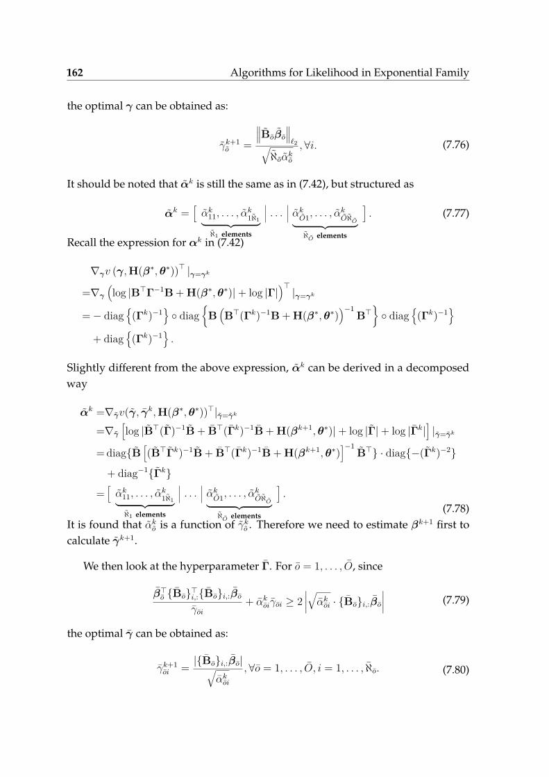
162 Algorithms for Likelihood in Exponential Family
the optimal γ can be obtained as:
γk+1o =
∥∥∥Boβo
∥∥∥ℓ2√
ℵoαko
,∀i. (7.76)
It should be noted that αk is still the same as in (7.42), but structured as
αk =[
αk11, . . . , αk
1ℵ1︸ ︷︷ ︸ℵ1 elements
. . . αkO1, . . . , αk
OℵO︸ ︷︷ ︸ℵO elements
]. (7.77)
Recall the expression for αk in (7.42)
∇γv (γ, H(β∗, θ∗))⊤ |γ=γk
=∇γ
(log |B⊤Γ−1B + H(β∗, θ∗)|+ log |Γ|
)⊤|γ=γk
=− diag{(Γk)−1
}◦ diag
{B(B⊤(Γk)−1B + H(β∗, θ∗)
)−1B⊤
}◦ diag
{(Γk)−1
}+ diag
{(Γk)−1
}.
Slightly different from the above expression, αk can be derived in a decomposedway
αk =∇γv(γ, γk, H(β∗, θ∗))⊤|γ=γk
=∇γ
[log |B⊤(Γ)−1B + B⊤(Γk)−1B + H(βk+1, θ∗)|+ log |Γ|+ log |Γk|
]|γ=γk
= diag{B[(B⊤Γk)−1B + B⊤(Γk)−1B + H(βk+1, θ∗)
]−1B⊤} · diag{−(Γk)−2}
+ diag−1{Γk}
=[
αk11, . . . , αk
1ℵ1︸ ︷︷ ︸ℵ1 elements
. . . αkO1, . . . , αk
OℵO︸ ︷︷ ︸ℵO elements
].
(7.78)It is found that αk
o is a function of γko . Therefore we need to estimate βk+1 first to
calculate γk+1.
We then look at the hyperparameter Γ. For o = 1, . . . , O, since
β⊤o {Bo}⊤
i,:{Bo}i,:βo
γoi
+ αkoiγoi ≥ 2
∣∣∣∣√αkoi · {Bo}i,:βo
∣∣∣∣ (7.79)
the optimal γ can be obtained as:
γk+1oi = |{Bo}i,:βo|√
αkoi
,∀o = 1, . . . , O, i = 1, . . . , ℵo. (7.80)

7.5 Optimisation Algorithm with Structural Sparsity 163
And αk is defined as
αk =[
αk11, . . . , αk
1ℵ1︸ ︷︷ ︸ℵ1 elements
. . . αkO1, . . . , αk
Oℵo︸ ︷︷ ︸ℵO elements
]. (7.81)
It should be noted that, we can obtain the following analytic form for the negativegradient of v(γ) at γ using basic principles in convex analysis as (using chain rule):
αk =∇γv(γk, γ, H(β∗, θ∗))⊤|γ=γk
=∇γ
[log |B⊤(Γk)−1B + B⊤Γ−1B + H(βk+1, θ∗)|+ log |B⊤ΓkB|+ log |Γ|
]|γ=γk
= diag{B[B⊤(Γk)−1B + B⊤(Γk)−1B + H(βk+1, θ∗)
]−1B⊤} · diag{−(Γk)−2}
+ diag−1{Γk}=[
αk11, . . . , αk
1ℵ1︸ ︷︷ ︸ℵ1 elements
. . . αkO1, . . . , αk
Oℵo︸ ︷︷ ︸ℵO elements
].
(7.82)It is found that αk
oi is a function of γkoi. Therefore we need to estimate βk+1
o first tocalculate γk+1
oi .
Two new variables related to weights are defined:
wko ≜
√√√√√ ℵo∑i=1
αkoi, (7.83)
and
wkoi ≜
√αk
oi, (7.84)
The pseudo code is summarised in Algorithm 14.
Similarly, we can derive the reweighted generalised fused group ℓ2 type algorithm.The pseudo code is summarised in Algorithm 15.
Similarly, let B be an identity matrix
B1
. . .
BO
=
I1
. . .
IO
.
The pseudo code is summarised in Algorithm 16.

164 Algorithms for Likelihood in Exponential Family
Algorithm 14 Reweighted Generalised Fused Group ℓ1 type algorithm for likelihoodin exponential family
1: Symbolic cache likelihood, gradient and Hessian expressions
p(y|β, θ) = a(θ) · exp{−E(β, θ)}; g(β, θ) = ∇E(β, θ); H(β, θ) = ∇∇E(β, θ);
2: Initialise the unknown hyperparameter γ1 as a unit vector;3: Fix/given the known parameter of the exponential family θ = θ∗;4: Initialise w1
o = 1, w1oi = 1, ∀i;
5: Fix λ = 1 and λ = 1 or select λ ∈ R+ and λ ∈ R+ as trail and error which may beempirically helpful;
6: for k = 1, . . . , kmax do7: Solve the following Fused Group Lasso type algorithm
βk+1 = argminβ
E(β, θ∗) + λO∑
o=1
∥∥∥wko · Boβo
∥∥∥ℓ2
+ λO∑
o=1
ℵo∑i=1
∥∥∥wkoi · {Bo}i,:βo
∥∥∥ℓ1
;
(7.85)
8: γk+1o =
∥Boβk+1o ∥ℓ2
wko
, and γk+1 =[
γk+11 , . . . , γk+1
1︸ ︷︷ ︸ℵ1 elements
. . . γk+1O
, . . . , γk+1O︸ ︷︷ ︸
ℵO elements
];
9: γk+1oi = |{Bo}i,:β
k+1o |
wkoi
, and γk+1 =[
γk+111 , . . . , γk+1
1ℵ1︸ ︷︷ ︸ℵ1 elements
. . . γk+1O1 , . . . , γk+1
OℵO︸ ︷︷ ︸ℵO elements
];
10: Ck+1 =(B⊤(Γk+1)−1B + B⊤(Γk+1)−1B + H(βk+1, θ∗)
)−1;
11: αk+1oi = −{Bo}i,:Ck+1{Bo}⊤
i,:(γk+1
o )2 + 1γk+1
o
;
12: wk+1o =
√∑ℵoi=1 αk+1
oi , ∀o = 1, . . . , O;
13: αk+1oi = −{Bo}i,:Ck+1{Bo}⊤
i,:(γk+1
o )2 + 1γk+1
o
;
14: wk+1oi =
√αk+1
oi , ∀o = 1, . . . , O, i = 1, . . . , ℵo;15: if a stopping criterion is satisfied then16: Break;17: end if18: end for
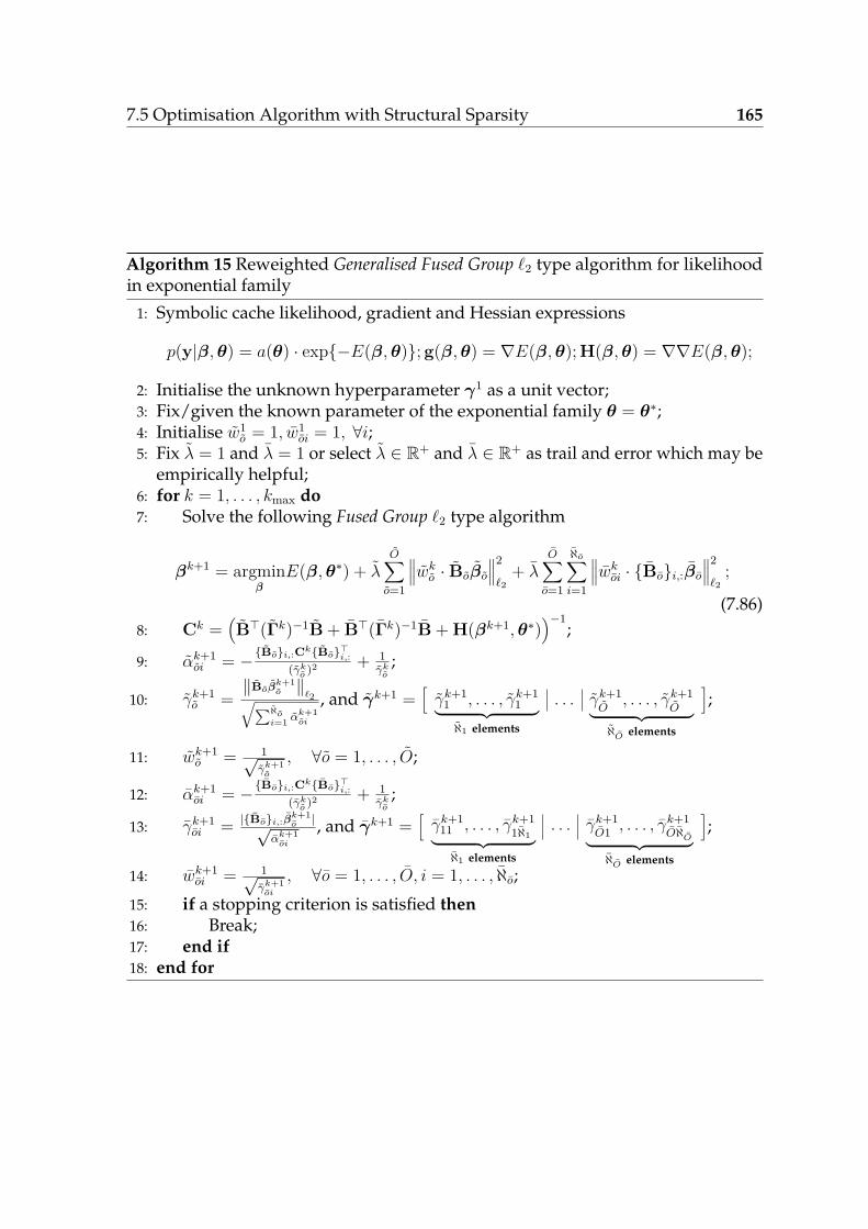
7.5 Optimisation Algorithm with Structural Sparsity 165
Algorithm 15 Reweighted Generalised Fused Group ℓ2 type algorithm for likelihoodin exponential family
1: Symbolic cache likelihood, gradient and Hessian expressions
p(y|β, θ) = a(θ) · exp{−E(β, θ)}; g(β, θ) = ∇E(β, θ); H(β, θ) = ∇∇E(β, θ);
2: Initialise the unknown hyperparameter γ1 as a unit vector;3: Fix/given the known parameter of the exponential family θ = θ∗;4: Initialise w1
o = 1, w1oi = 1, ∀i;
5: Fix λ = 1 and λ = 1 or select λ ∈ R+ and λ ∈ R+ as trail and error which may beempirically helpful;
6: for k = 1, . . . , kmax do7: Solve the following Fused Group ℓ2 type algorithm
βk+1 = argminβ
E(β, θ∗) + λO∑
o=1
∥∥∥wko · Boβo
∥∥∥2
ℓ2+ λ
O∑o=1
ℵo∑i=1
∥∥∥wkoi · {Bo}i,:βo
∥∥∥2
ℓ2;
(7.86)8: Ck =
(B⊤(Γk)−1B + B⊤(Γk)−1B + H(βk+1, θ∗)
)−1;
9: αk+1oi = −{Bo}i,:Ck{Bo}⊤
i,:(γk
o )2 + 1γk
o;
10: γk+1o =
∥Boβk+1o ∥ℓ2√∑ℵo
i=1 αk+1oi
, and γk+1 =[
γk+11 , . . . , γk+1
1︸ ︷︷ ︸ℵ1 elements
. . . γk+1O
, . . . , γk+1O︸ ︷︷ ︸
ℵO elements
];
11: wk+1o = 1√
γk+1o
, ∀o = 1, . . . , O;
12: αk+1oi = −{Bo}i,:Ck{Bo}⊤
i,:(γk
o )2 + 1γk
o;
13: γk+1oi = |{Bo}i,:β
k+1o |√
αk+1oi
, and γk+1 =[
γk+111 , . . . , γk+1
1ℵ1︸ ︷︷ ︸ℵ1 elements
. . . γk+1O1 , . . . , γk+1
OℵO︸ ︷︷ ︸ℵO elements
];
14: wk+1oi = 1√
γk+1oi
, ∀o = 1, . . . , O, i = 1, . . . , ℵo;
15: if a stopping criterion is satisfied then16: Break;17: end if18: end for

166 Algorithms for Likelihood in Exponential Family
Algorithm 16 Reweighted Fused Group ℓ1 type algorithm for likelihood in exponen-tial family
1: Symbolic cache likelihood, gradient and Hessian expressions
p(y|β, θ) = a(θ) · exp{−E(β, θ)}; g(β, θ) = ∇E(β, θ); H(β, θ) = ∇∇E(β, θ);
2: Initialise the unknown hyperparameter γ1 as a unit vector;3: Fix/given the known parameter of the exponential family θ = θ∗;4: Initialise w1
o = 1, w1oi = 1, ∀i;
5: Fix λ = 1 and λ = 1 or select λ ∈ R+ and λ ∈ R+ as trail and error which may beempirically helpful;
6: for k = 1, . . . , kmax do7: Solve the following Fused Group Lasso type algorithm
βk+1 = argminβ
E(β, θ∗) + λO∑
o=1
∥∥∥wko · βo
∥∥∥ℓ2
+ λO∑
o=1
ℵo∑i=1
∥∥∥wkoi · {Bo}i,:βo
∥∥∥ℓ1
;
(7.87)
8: γk+1o =
∥βk+1o ∥ℓ2wk
o, and γk+1 =
[γk+1
1 , . . . , γk+11︸ ︷︷ ︸
ℵ1 elements
. . . γk+1O
, . . . , γk+1O︸ ︷︷ ︸
ℵO elements
];
9: γk+1oi = |{Bo}i,:β
k+1o |
wkoi
, and γk+1 =[
γk+111 , . . . , γk+1
1ℵ1︸ ︷︷ ︸ℵ1 elements
. . . γk+1O1 , . . . , γk+1
OℵO︸ ︷︷ ︸ℵO elements
];
10: Ck+1 =((Γk+1)−1 + B⊤(Γk+1)−1B + H(βk+1, θ∗)
)−1;
11: αk+1o = − Ck+1
(γk+1o )2 + 1
γk+1o
;
12: wk+1o =
√ℵo · αk+1
o ;
13: αk+1oi = −{Bo}i,:Ck+1{Bo}⊤
i,:(γk+1
o )2 + 1γk+1
o
;
14: wk+1oi =
√αk+1
oi ;15: if a stopping criterion is satisfied then16: Break;17: end if18: end for

7.5 Optimisation Algorithm with Structural Sparsity 167
Algorithm 17 Reweighted Fused Group ℓ2 type algorithm for likelihood in exponen-tial family
1: Symbolic cache likelihood, gradient and Hessian expressions
p(y|β, θ) = a(θ) · exp{−E(β, θ)}; g(β, θ) = ∇E(β, θ); H(β, θ) = ∇∇E(β, θ);
2: Initialise the unknown hyperparameter γ1 as a unit vector;3: Fix/given the known parameter of the exponential family θ = θ∗;4: Initialise w1
o = 1, w1oi = 1, ∀i;
5: Fix λ = 1 and λ = 1 or select λ ∈ R+ and λ ∈ R+ as trail and error which may beempirically helpful;
6: for k = 1, . . . , kmax do7: Solve the following Fused Group ℓ2 type algorithm
βk+1 = argminβ
E(β, θ∗) + λO∑
o=1
∥∥∥wko · βo
∥∥∥2
ℓ2+ λ
O∑o=1
ℵo∑i=1
∥∥∥wkoi · {Bo}i,:βo
∥∥∥2
ℓ2;
(7.88)8: Ck =
((Γk)−1 + B⊤(Γk)−1B + H(βk+1, θ∗)
)−1;
9: αk+1o = − Ck
(γko )2 + 1
γko
;
10: γk+1o =
∥βk+1o ∥ℓ2√ℵo·αk+1
o
, and γk+1 =[
γk+11 , . . . , γk+1
1︸ ︷︷ ︸ℵ1 elements
. . . γk+1O
, . . . , γk+1O︸ ︷︷ ︸
ℵO elements
];
11: wk+1o = 1√
γk+1o
;
12: αk+1oi = −{Bo}i,:Ck{Bo}⊤
i,:(γk
o )2 + 1γk
o;
13: γk+1oi = |{Bo}i,:β
k+1o |√
αk+1oi
, and γk+1 =[
γk+111 , . . . , γk+1
1ℵ1︸ ︷︷ ︸ℵ1 elements
. . . γk+1O1 , . . . , γk+1
OℵO︸ ︷︷ ︸ℵO elements
];
14: wk+1oi = 1√
γk+1oi
;
15: if a stopping criterion is satisfied then16: Break;17: end if18: end for

168 Algorithms for Likelihood in Exponential Family
Similarly, we can derive the reweighted fused group ℓ2 type algorithm. The pseudocode is summarised in Algorithm 17.
Remark 20 (Remark on Algorithms in Section 7.5) If the Algorithms in Section needsto be efficiently implemented like the one in Algorithm 9. The Maximum a Posteriorprocedure, a.k.a.,the argmin step, in the ℓ2 type Algorithms, can be similarly substituted bythe “inner for loop” procedures in Algorithm 9. More specifically, these Algorithms includeAlgorithm 11, 13, 15, 17.
Remark 21 (Remark on the extension to train deep neural networks) A possible andintuitive algorithm extension to train deep neural networks with structural sparsity can befound later in Section 14.1.2 and 14.1.4 of Chapter 14.

Chapter 8
Algorithms for Online ModelSelection

170 Algorithms for Online Model Selection
Our method allows inference of model structures that can be decomposed aslinear combinations of nonlinear functions chosen from a dictionary set. We note,however, that the identification of parameters nonlinearly embedded in these func-tions is a non-trivial task. As we saw in the previous section, a naive approachconsists in augmenting the set of dictionary functions with various candidate non-linearities for which nonlinearly embedded parameters are given specific values.We would then rely on the approximation of the true nonlinearities as a linear com-bination of these dictionary functions, i.e. on estimating the true nonlinearity as an“interpolation” from discretely valued candidate nonlinearities.
On the other hand, filtering methods have been widely used to estimate parame-ters for a given (nonlinear) parametric structure [209]. The main issue with filteringmethods is that they require a priori knowledge of such model structures and cannoteasily be used to infer model structures in other ways than by trying individualstructures and comparing them using model selection criteria. Typically, this processhas a very high computational cost.
In the following section, we show how our model structure inference (describedin Algorithm 5) can be used to identify nonlinear terms that can benefit from furtherrefinement using filtering approaches. For example, if the right hand side of oneof the equations in the identified model was to contain a linear combination of theform 0.2684
1+x+ 0.7292
1+x3 , a new parametric structure could be created where this termis replaced by Vmax
K+xh . This new parametric model structure can then serve as thestarting point for filtering methods, which are then used to estimate the values of theparameters in the new parametric structure. Furthermore, the parameters identifiedusing our model structure inference method can be used as initial guesses or priorsfor the filtering methods.
8.1 Extended Kalman Filter
As mentioned above, our model structure inference method can be used to identifynonlinear terms that can benefit from further refinement in their structure. Let thenew parametric structure obtained through such refinement be given by:
xt+1 = g(xt, ut, γ) + ξt,
zt = xt + ηt,
x1 = g0,
(8.1)

8.1 Extended Kalman Filter 171
where g0 is the initial guess of the state vector x.
Extended or unscented Kalman filtering are celebrated methods used to identifyboth the state variables in x and the parameters in γ of a given parametric modelstructure such as the one provided in (8.1). Simultaneous identification of statevariables and parameters can be done using a “state extension” approach whereconstant parameters such as those contained in the model parameter vector γ areconsidered as additional state variables with a rate of change equal to zero. In thisway, constant parameters are treated as constant functions of time as opposed toconstant numbers [200].
The parameters identified using our model structure inference method (seeAlgorithm 5) can be used as initial guesses or priors for the parameters γ.
Filtering can be made more tractable by considering that the unknown parame-ters γ evolve according to a Brownian motion. For this, we introduce a new variableϕk and consider the following linear process model:
ϕt+1
γt+1
= I 0∆τ I
ϕt
γt
+ ϱt , (8.2)
where ϱt has covariance:
Qϱ := σ2
∆τ ∆τ 2/2∆τ 2/2 ∆τ 3/3
,
where σ2 must be chosen a priori. We further define the augmented state parametricstructure as:
xt ≜
xt
ϕt
γt
, g(xt, ut) ≜
g(xt, ut, γt)
ϕt
γt + ∆tϕt
,
ξt ≜ ξt
ϱt
, g0 ≜
g0
ϕ0
γ0
,
(8.3)
where g0 is the initial state estimate.
We can now write the full augmented dynamic model as
xt+1 = g(xt, ut) + ξt,
zt = [Inx , 0]xt + ηt,
x1 = g0.
(8.4)

172 Algorithms for Online Model Selection
The new process noise ξt has positive definite covariance matrix
Qt = Qt 0
0 Qϱ
.
Using such a state extension approach, the problem of parameter estimation isconverted into a problem of state estimation, for which the goal is to estimate theextended state x from measurements of the output z. More precisely, we are tryingto determine the initial conditions g0, which, when used to initialise the system (8.1),generates the observed output z.
8.2 Algorithm combining model structure identificationand model refinement
In this section we present Algorithm 18, which constitutes the main algorithmcombining 1) our model structure identification method (Algorithm 5) with 2) modelrefinement of model structures using filtering. Model structure identification is doneoff-line and thus requires batched data (historical sensor measurements) which werecollected a priori. Once a ‘rough’ model structure is obtained, model refinement canbe performed on-line by feeding streaming data (sensor measurements that arrive inreal-time).
In Algorithm 18, we define a trial as the application of the model structureidentification procedure described in Algorithm 5 using a given set of dictionaryfunctions and a given regularisation parameter λ.

8.2 Algorithm combining model structure identification and model refinement 173
Algorithm 18 Online Model Selection Algorithm
1: IDENTIFICATION:Require: Batched Data
2: procedure IDENTIFICATION(S trials)3: for s = 1, . . . , S do4: Choose a regularisation parameter λs;5: Choose a set of dictionary functions;6: Using the set of dictionary functions, construct Xs from batched data;7: Ms = IDENTIFICATION(λs, Xs); % Apply Algorithm 5to get a modelMs;
8: end for9: Pick the top S rankedMs models based on a certain model selection criterion.
10: end procedure11: Update:12: procedure UPDATE(S trials)13: Update candidate functions as stated in the introduction to Section 8.1;14: end procedure15: FILTERING:Require: Streaming Data16: procedure FILTERING(S trials)17: while New data zt is available do18: for s = 1, . . . , S do19: Mnew
s = FILTERING(zt); % Apply Filtering techniques to refinemodelMs
20: end for21: end while22: if Not convergent then goto IDENTIFICATION23: end if24: end procedure


Chapter 9
Algorithms for Fault Diagnosis

176 Algorithms for Fault Diagnosis
9.1 Fault Diagnosis Problem Formulation
We slightly change the notation of the linear regression model (4.28) in Chapter 4.5.2.we can write (4.28) into a vector form:
ei(t + 1) = fi(x(t))βtruei + ηi(t), (9.1)
with
fi(x(t)) = [fi1(x(t)), . . . , fiN(x(t))] ∈ RN , (9.2)
βtruei = [βi1, . . . , βiN ]⊤ ∈ RN . (9.3)
As stated in Definition 2, if there are no faults occurring in the system, thedynamics of the system will evolve according to (9.1). The e
¯xpected output for the
next sampling time is defined to be
e[e]i (t + 1) = fi(x(t))βtrue
i . (9.4)
From (9.1) and (9.4), it is easy to show that ei(t + 1) − e[e]i (t + 1) is a stochastic
variable with zero mean and variance σ2. If there are faults occurring in the system,the corresponding weights will change from βtrue
i to βfaulti . Similar to the definition
of βtruei , βfault
i = [β[f ]i1 , . . . , β
[f ]iN ]⊤. We thus have:
e[f ]i (t + 1) = fi(x(t))βfault
i + ηi(t), (9.5)
where e[f ]i is the output when there are f
¯aults.
From (9.4) and (9.5), it is easy to find that e[f ]i (t + 1) − e
[e]i (t + 1) is a stochastic
variable with mean: fi(x(t))(βfaulti − βtrue
i )variance: σ2
Denotingyi = e
[f ]i − e
[e]i , βi = βfault
i − βtruei ,
we have:yi(t + 1) = fi(x(t))βi + ηi(t). (9.6)

9.2 Fault Detection and Isolation Algorithm 177
Remark 22 We formulate the faults identification problem as a linear regression problem.The dependent variable e
[f ]i (t + 1)− e
[e]i (t + 1) is the difference between the expected output
and the faulty output; the unknown variable we want to estimate is the difference betweenthe faulty transmission weights and the true transmission weights.
9.2 Fault Detection and Isolation Algorithm
There are three problems of interest based on the formulation in (9.6): a) detectionof a fault; b) isolation of a fault, i.e. determination of the type, location and time ofoccurrence of a fault; and c) identification of the size and time-varying behaviour ofa fault. In the noiseless case, when there are no faults, ∀i, yi and βi are both equalto zero. On the other hand, when there are faults, certain yi are nonzero. So thefaults can be detected by identifying the entries yi that are nonzero. However, in thenoisy case, even when there are no faults, yi is nonzero most of the time since it is astochastic variable with zero mean. This can be interpreted in a probabilistic way byChebyshev’s Inequality:
p(|ei(t + 1)− e[e]i (t + 1)| ≥ lσ = σ∗) ≤ 1
l2
where l ∈ R+. According to this inequality, when there are no faults, the deviationbetween true and expected outputs, i.e. |ei(t + 1) − e
[e]i (t + 1)| cannot be much
greater than zero with high probability. On the other hand, when there is a fault, thedeviation between faulty and expected outputs, i.e. |e[f ]
i (t + 1)− e[e]i (t + 1)| should
be much greater than zero with high probability.
From an isolation point of view and Chebyshev’s inequality, when |e[f ]i (t + 1)−
e[e]i (t + 1)| is much greater than σ, the fault can be isolated with high probability (e.g.
if the threshold is set to lσ = 10σ, then the probability is 99%).
9.3 Fault Identification Algorithm
If at time t1 faults have been detected and isolated, the remaining task is to performfault identification, i.e. to identify the location of the faults or equivalently to find thenonzero entries in βi. Assuming that M successive data points, including the initial

178 Algorithms for Fault Diagnosis
data point at t1, are sampled and defining
yi ≜ [yi(t1), . . . , yi(M)]⊤ ∈ RM ,
Xi ≜
fi(x(t1))
...fi(x(M))
∈ RM×N ,
ηi ≜ [ηi(t1), . . . , ηi(M)]⊤ ∈ RM ,
(9.7)
we can write N independent equations of the form:
yi = Xiβi + ηi, i = 1, . . . , N. (9.8)
Based on the formulation in (9.8), our goal is to find βi given the output datastored in yi. y is the difference between the faulty measurements and the expectedmeasurements, or namely, the error measurements; and β is the difference betweenthe faulty parameters and the true parameters, or namely, the faults. We addressthis linear regression problem under the following assumption.
Assumption 10 A maximum of S system parameters are faulty, i.e. βi has at most S
non-zero entries. In other words, βi is S-sparse or mathematically, ∥βi∥ ≤ S. The constantS is assumed unknown to the system administrator.
On the other-hand, the size of y equals to the number of samples needed toidentify the location of the faults after the they occur. From a practical viewpoint,the number of samples should be as small as possible. However, standard leastsquare approaches to (9.7) cannot meet this goal as they require at least 2N samples.Moreover, the solution to the standard least square problem is generically dense(hence, violating Assumption 10) and cannot be used to identify which transmissionlines are likely to be faulty by identification of the nonzero entries of the estimatedβfault − βtrue.
Based on Algorithm 3, we can summarise the fault diagnosis algorithm in Algo-rithm 19.

9.3 Fault Identification Algorithm 179
Algorithm 19 Fault Diagnosis Algorithm
1: Set a threshold σ∗ as indicated in Section 9.2, e.g. σ∗ = 10× σ;2: for k = 0, . . . , T do3: % T is an integer indicating the number of diagnosis rounds;4: for i = 1, . . . , N do5: Collect the output data ei(t + 1) in (9.1);6: Calculate the expected output e
[e]i (t + 1) in (9.4);
7: if |ei(t + 1)− e[e+]i (t + 1)| > σ∗ then
8: Fault is detected for βi; % {fault detection procedure}9: Compute yi(t + 1) in (9.6);
10: if |yi(t + 1)| > σ∗ then11: Isolate fault i; % {fault isolation procedure}12: end if13: end if14: Set M ← k;15: Apply Algorithms propose in Chapter 6.6 to identify the faults βi; % {fault
identification procedure}16: end for17: if ∀i, ∥βi∥0 converge to some constant then18: Break;19: end if20: end for21: An estimate for the faults β in (9.8), i = 1, . . . , N .


Part III
Applications


Chapter 10
Biochemical Reaction NetworkIdentification

184 Biochemical Reaction Network Identification
10.1 Identification from Single Time Series Data
In this example, we consider a classical dynamical system in systems/syntheticbiology, the repressilator, which we use to illustrate the reconstruction problemat hand. The repressilator is a synthetic three-gene regulatory network where thedynamics of mRNAs and proteins follow an oscillatory behaviour [55]. A discrete-time mathematical description of the repressilator, which includes both transcriptionand translation dynamics, is given by the following set of discrete-time equations:
x1(t + 1)− x1(t)∆t
= −γ1x1(t) + α1
(1 + xn16 (t)) + ξ1(t),
x2(t + 1)− x2(t)∆t
= −γ2x2(t) + α2
(1 + xn24 (t)) + ξ2(t),
x3(t + 1)− x3(t)∆t
= −γ3x3(t) + α3
(1 + xn35 (t)) + ξ3(t),
x4(t + 1)− x4(t)∆t
= −γ4x4(t) + β1x1(k) + ξ4(t),
x5(t + 1)− x5(t)∆t
= −γ5x5(k) + β2x2 + ξ5(t),
x6(t + 1)− x6(t)∆t
= −γ6x6(t) + β3x3(t) + ξ6(t).
Here, x1, x2, x3 (resp. x4, x5, x6) denote the concentrations of the mRNA transcripts(resp. proteins) of genes 1, 2, and 3, respectively. ξi, ∀i are i.i.d. Gaussian noise.α1, α2, α3 denote the maximum promoter strength for their corresponding gene,γ1, γ2, γ3 denote the mRNA degradation rates, γ4, γ5, γ6 denote the protein degra-dation rates, β1, β2, β3 denote the protein production rates, and n1, n2, n3 the Hillcoefficients. The set of equations in (10.1) corresponds to a topology where gene 1 isrepressed by gene 2, gene 2 is repressed by gene 3, and gene 3 is repressed by gene 1.Take gene 1 for example. The hill coefficient n1 will typically have a value within arange from 1 to 4 due to biochemical constraints. The core question here is: how canwe determine the topology and kinetic parameters of the set of equations in (10.1)from time series data of x1, . . . , x6?
Note that we do not assume a priori knowledge of the form of the nonlinearfunctions appearing on the right-hand side of the equations in (10.1), e.g., whetherthe degradation obeys fi rst-order or enzymatic catalysed dynamics or whether theproteins are repressors or activators. It should also be noted that many linear andnonlinear functions can be used to describe the dynamics of GRNs in terms of bio-chemical kinetic laws, e.g., first-order functions f([S]) = [S], mass action functions

10.1 Identification from Single Time Series Data 185
f([S1] , [S2]) = [S1] · [S2], Michaelis-Menten functions f([S]) = Vmax [S] /(KM + [S]),or Hill functions f([S]) = Vmax [S]n /(Kn
M + [S]n). These kinetic laws typical of bio-chemistry and GRN models will aid in the definition of the dictionary functionmatrix. Next we show how the network construction problem of the repressilatormodel in (10.1) can be formulated in a linear regression form.
We construct a candidate dictionary matrix X, by selecting as candidate basisfunctions, nonlinear functions typically used to represent terms appearing in bio-chemical kinetic laws of GRN models. As a proof of concept, we only considerHill functions as potential nonlinear candidate functions. The set of Hill functionswith Hill coefficient h, both in activating and repressing from, for each of the 6 statevariables are:
hillh(t) ≜[
11 + xh
1(t) , . . . ,1
1 + xh6(t) ,
xh1(t)
1 + xh1(t) , . . . ,
xh6(t)
1 + xh6(t)
]1×12
, (10.1)
where h represents the Hill coefficient. In what follows we consider that the Hillcoefficient can take any of the following integer values: 1, 2, 3 or 4. Since there are 6state variables, we can construct the dictionary matrix X with 6 (dictionary functionsfor linear terms) +(4 ∗ 12) (dictionary functions for Hill functions) = 54 columns.
X =
x1(0) . . . x6(0) hill1(0) . . . hill4(0)
......
......
x1(M − 1) . . . x6(M − 1) hill1(M − 1) . . . hill4(M − 1)
∈ RM×(6+48).
(10.2)Then the output can be defined as
yi ≜[
xi(1)− xi(0)∆t
, . . . ,xi(M)− xi(M − 1)
∆t
]⊤
∈ RM×1, i = 1, . . . , 6.

186 Biochemical Reaction Network Identification
Considering the dictionary matrix X given in (10.2), the corresponding target βi forthe “correct” model in (10.1) should be:
βtrue = [β1, β2, β3, β4, β5, β6] =
−γ1(= −0.3) 0 0 β1(= 1.4) 0 00 −γ2(= −0.4) 0 0 β2(= 1.5) 00 0 −γ3(= −0.5) 0 0 β3(= 1.6)0 0 0 −γ4(= −0.2) 0 00 0 0 0 −γ5(= −0.4) 00 0 0 0 0 −γ6(= −0.6)
047×1 045×1 046×1
α1(= 4) α2(= 3) α3(= 5) 048×1 048×1 048×1
00×1 02×1 01×1
.
(10.3)
with values in brackets indicating the correct parameter values.
To generate the time-series data, we took ‘measurements’ every 1 unit betweent = 0 and t = 50 (arbitrary units) from random initial conditions which are drawnfrom a standard uniform distribution on the open interval (0, 1). Thus a total of 51measurements for each state are collected (including the initial value). It should benoted that the number of rows is less than the number of columns in the dictionarymatrix.
We here investigate the performance of various algorithms including ours (Algo-rithm 1 in the main text) for different signal-to-noise ratios of the data. We definethe signal-to-noise ratio (SNR) as
SNR(dB) ≜ 20 log10∥Xβtrue∥2
∥Ξ∥2.
We considered SNRs ranging from 0 dB to 25 dB for each generated weight. Tocompare the reconstruction accuracy of the various algorithms considered, we usethe root of normalised mean square error (RNMSE) as a performance index, i.e.
∥βestimate − βtrue∥2
∥βtrue∥2(10.4)
For each SNR, we performed 200 independent experiments and calculated theaverage RNMSE for each SNR over these 200 experiments. In each “experiment”,we simulated the repressilator model with random initial conditions drawn froma standard uniform distribution on the open interval (0, 1). The parameters were
10.1 Identification from Single Time Series Data 187
drawn from a standard uniform distribution with the true values βtrue in (10.3) takenas the mean and variations around the mean values no more than 10% of the truevalues. In MATLAB, one can use βtrue.*(0.9 + 0.2*rand(54,6)) to generatethe corresponding parameter matrix for each experiment.
Based on these settings, we compared Algorithm 4 with nine other state-of-the-art sparse linear regression algorithms available at [54]. [54] provides accessto a free MATLAB software package managed by David Donoho and his team andcontains various tools for finding sparse solutions of linear systems, least-squareswith sparsity, various pursuit algorithms, and more. We compare our identifica-tion algorithm with nine other state-of-the-art sparse linear regression algorithmsavailable at [54], namely, BP (Basis Pursuit), IRWLS (Iteratively ReWeighted LeastSquares), ISTBlock (Iterative Soft Thresholding, block variant with least squares pro-jection), LARS (Least-Angle RegreSsion), MP (Matching Pursuit), OMP (OrthogonalMatching Pursuit), PFP (Polytope Faces Pursuit), Stepwise (Forward Stepwise), andStOMP (Stagewise Orthogonal Matching Pursuit).
In Fig. 10.1, we plot, for various SNRs, the average RNMSE obtained using ourcentralised algorithm (both implementation using the generic parser CVX and cen-tralised ADMM implementations) and other algorithms in [54]. In Fig. 10.2, we plot,for the various SNRs considered, the average computational running time requiredby our algorithm and the other algorithms from [54]. During this comparison, theinputs for the algorithms listed in these algorithms are always the same, i.e. thedictionary matrix X and the data contained in y. The initialisation and pre-specifiedparameters for these algorithms were set to their default values provided in [54].Interested readers can download the package from [54] and reproduce the resultspresented here under the default settings of the solvers therein.
It should be noted that the dictionary matrices in all the experiments are rankdeficient, i.e. neither column rank nor row rank are full. As a consequence, boththe MP and OMP algorithm fail to converge or yield results with extremely largeRNMSE. As these two algorithms cannot satisfactorily be used, they have beenremoved from the comparison results presented in Fig. 10.1 and Fig. 10.2. It can beseen from Fig. 10.1 that our algorithm outperforms all the other algorithms in [54] interms of RNMSE.

188 Biochemical Reaction Network Identification
0 5 10 15 20 2510
−4
10−3
10−2
10−1
100
101
102
103
RNMSE Comparision: Genetic Repressilator in Example 2
SNR (dB)
RN
MS
E
Our AlgorithmBPIRWLSISTBlockLARSPFPStepwiseStOMP
Fig. 10.1 Root of Normalised Mean Square Error ∥βestimate − βtrue∥2/∥βtrue∥2 averagedover 200 independent experiments for the signal-to-noise ratios 0 dB, 5 dB, 10 dB, 15dB, 20 dB, and 25 dB.
0 5 10 15 20 25 3010
−3
10−2
10−1
100
101
102
Computational Running Time Comparision: Genetic Repressilator in Example 2
SNR (dB)
Com
puta
tiona
l Run
ning
Tim
e (s
econ
ds)
Our AlgorithmBPIRWLSISTBlockLARSPFPStepwiseStOMP
Fig. 10.2 Computational running time averaged over 200 independent experimentsfor the signal-to-noise ratios 0 dB, 5 dB, 10 dB, 15 dB, 20 dB, and 25 dB.
10.2 Identificaton from Multiple Heterogeneous Time Series Datasets 189
10.2 Identificaton from Multiple Heterogeneous TimeSeries Datasets
In this Section, we use numerical simulations to show the effectiveness of the pro-posed algorithm. To compare the identification accuracy of the various algorithmsconsidered, we use the root of normalised mean square error (RNMSE) as a perfor-mance index, i.e.
RNMSE = ∥βestimate − βtrue∥2
∥βtrue∥2.
Several factors affect the RNMSE, e.g. number of experiments C, measurementnoise intensity, dynamic noise intensity, length of single time series data M , numberof candidate basis functions N . For brevity of exposition, we only show resultspertaining to change of RNMSE over number of experiment C and length of singletime series for one experiment, all in the noiseless case. More results related toother factors that may affect RNMSE will be shown in a future journal publicationpresenting these results in more details.
As an illustrative example, we consider a model of an eight species generalisedrepressilator [181], which is a system where each of the species represses anotherspecies in a ring topology. The corresponding dynamic equations are as follows:
x1t = p11
pp1312 + xp13
8t
+ p14 − p15x1t,
xit = pi1
ppi3i2 + xpi3
i−1,t
+ pi4 − pi5xit, ∀i = 2, . . . 8,(10.5)
where pij , i = 1, . . . , 8, j = 1, . . . , 5. We assume the mean value for these parametersacross different species and experiments are pi1 = 40, pi2 = 1, pi3 = 3, pi4 = 0.5, pi5 =1, ∀i. We simulate the ODEs in Eq. (10.5) to generate the time series data. In each“experiment” or simulation of Eq. (10.5), the initial conditions are randomly drawnfrom a standard uniform distribution on the open interval (0, 1). The parametersin each experiment vary no more than 20% of the mean values. In MATLAB, onecan use pij*(0.8 + 0.4*rand(1)) to generate the corresponding parameters foreach experiment.
The numerical simulation procedure can be summarised as follows:
1. The deterministic system of ODEs (10.5) is solved numerically with an adaptivefourth-order Runge-Kutta method;

190 Biochemical Reaction Network Identification
X =
x1(1) . . . x8(1) hill(x1(1), 1, 0, 3) . . . hill(x8(1), 1, 3, 3) 1
......
......
...x1(M) . . . x8(M) hill(x1(M), 1, 0, 3) . . . hill(x8(M), 1, 3, 3) 1
∈ RM×25.
(10.7)
2. As explained in (5.14), Gaussian measurement noise with variance σ2 is addedto the corresponding time-series data obtained in the previous step1;
3. The data is re-sampled with uniform intervals2;
4. The local polynomial regression framework in [48] is applied to estimate thefirst derivative;
5. A dictionary matrix is constructed;
6. Algorithm in Chapter 3 is used to identify the model.
The candidate dictionary matrix X in step 5) above is constructed by selectingas candidate nonlinear basis functions typically used to represent terms appearingin ODE models of Gene Regulatory Networks. As a proof of concept, we onlyconsider Hill functions as potential nonlinear candidate functions. The set of Hillfunctions with Hill coefficient h, both in activating and repressing form, for the ith
state variables at time instant tk are:
hill(xi(t), K, hnum, hden) ≜ xhnumi (t)
Khden + xhdeni (t)
(10.6)
where hnum and hden represent the Hill coefficients. When hnum = 0, the Hill functionhas a repression form, whereas an activation form is obtained for hnum = hden = 0.
In our identification experiment, we assume hnum, hden and K to be known. Weare interested in identifying the regulation type (linear or Hill type, repression oractivation) and the corresponding parameters pi1, the degradation rate constantpi4 and the basal expression rate pi5, ∀i. Since there are 8 state variables, we canconstruct the dictionary matrix X with 8 (basis functions for linear terms) +(2 ∗ 8)(basis functions for Hill functions, both repression and activation form) +1 (constantunit vector) = 25 columns. The corresponding matrix X is given in Eq. (10.10)
1In the example presented here, we consider the noiseless case corresponding to σ = 0.2In this example, interval length is set to 1.

10.3 Online Model Selection 191
For a fixed number of experiments C and length of single time series M , we com-pute the RNMSE over 50 simulations by varying initial conditions and parameterspij . The RNMSE over C and M are shown in Fig. 10.3(a) and Fig. 10.3(b), using bothgroup Lasso and Algorithm 5 with the maximal iteration number kmax = 5 (see line4 in Algorithm 5). Inspection of the results presented in Fig. 10.3(a) and Fig. 10.3(b)clearly show that Algorithm 5 outperforms significantly group Lasso in terms ofRNMSE.
10.3 Online Model Selection
10.3.1 Background
Transcription and translation are two intrinsically slow processes (time scale of min-utes in bacteria). While, on one hand, this implies there is no stringent need to ob-serve cells with high sampling frequencies, it also means that identification/controlexperiments of biomolecular circuits usually last hours to days, i.e. much longer thansimilar experiments carried out on electrical or mechanical systems. Over such longtime frames it is necessary to (a) effectively trap cells and (b) observe their internaldynamics. We also need to extract single cell trajectories while we (c) stimulate themwith time-varying profiles of the molecules that serve as inducers for the network ofinterest. Most importantly it is necessary to achieve these objectives with minimallyinvasive techniques, i.e. using methods that ideally, will not affect the processes wewant to quantify (a point not to be overlooked as factors like heat, e.g. generatedby the light used to obtain microscopy images, or mechanical stresses, e.g. usedto physically hold cells in place while imaging them, will trigger stress responsesin cells). For these reasons we need to continuously (i) supply cells with nutrientsand (ii) remove toxic metabolites while (iii) retaining the ability to condition theirmicroenvironment to expose them to the appropriate externally applied stimuli.All these requirements, combined, significantly limit the technologies that can beused to identify and control biomolecular circuits in vivo: for example commonlyused methods, such as flask-based sampling or bioreactors, are unable to provideus with single cell trajectories. Microfluidics, enabling us to fabricate transparentmicrochannels where cells can be trapped and observed while being exposed to acontinuous flow of nutrients and chemicals controlled by a computer, does allow tomeet the requirements mentioned above.

192 Biochemical Reaction Network Identification
02
Number of experiemnt: C
46
810100Length of single time series: M
8060
4020
0.95
0.8
0.9
1
0.75
0.85
0
RN
MS
E
(a) Group Lasso (first iteration of Algorithm 5). The minimal RNMSE is around0.75
02
Number of experiemnt: C
46
810100Length of single time series: M
8060
4020
0.3
0
0.1
0.2
1
0.9
0.5
0.4
0.8
0.7
0.6
0
RN
MS
E
(b) Algorithm 5 with maximal iteration number kmax = 5. The minimalRNMSE is almost 0.
Fig. 10.3 Algorithm comparison in terms of RNMSE ∥βestimate − βtrue∥2/∥βtrue∥2 aver-aged over 50 independent experiments.

10.3 Online Model Selection 193
In the view of the above, we will consider the setup documented in [124] as thereference platform for the in vivo implementation of our model selection approach.In this configuration, described in Fig 10.4, a microfluidic device containing thecells carrying the network of interest, is mounted on the stage of a fully automatedmicroscope that takes phase contrast and fluorescence images of the cells at regulartime intervals. Such images are used by the computer to locate cells (phase contrast)and estimate the amount of protein (fluorescence imaging) in real-time via a customimage processing algorithm developed in MATLAB. The computer, then, uses a setof fluidic pressure actuators to vary the level of inducer the cells are exposed to.Interestingly, this configuration allows us to continuously (a) update our model on-line and, potentially, (b) automtically carry out multiple model-selection iterationswithin the same experiment, a unique feature of this approach [163].
Fig. 10.4 Technological platform for in-vivo model selection of synthetic circuits.In this closed loop configuration the computer (upper right corner) takes imagesof the cells in the microfluidic device (lower left corner) via a microscope (upperleft corner), quantifies the output of the network of interest in real time and appliesthe next sample of input(s) via the fluidic pressure actuation system (lower rightcorner).

194 Biochemical Reaction Network Identification
In order to extend the experimental throughput and increase our model discrim-ination capabilities we will use the MDAW microfluidic device described in [59]:in this device 8 independent model selection experiments can be carried out at thesame time. We will seed the same strain in each of the 8 chambers and image the 8chambers at regular intervals. In so doing we will obtain 8 independent datasets(each formed by an exponentially growing number of single cell trajectories) that wewill use to design and implement our model selection experiment.
Mathematical model
Throughout this Chapter, we will assume that the process of interest can be modelledby a discrete-time system of the form:
xt+1 = g(xt, ut, β) + ξt,
zt = xt + ηt,(10.8)
where the xt = [x1,t, . . . , xnx,t] ∈ Rnx is the state vector at discrete time point t; β
represents the vector of parameters to be identified; the function g : Rnx × Rnu ×Rnβ → Rnx is nonlinear and depends (explicitly) on the input vector ut ∈ Rnu . Theprocess noise ξt ∈ Rnx and measurement noise ηt ∈ Rnx are assumed to be mutuallyindependent Gaussian random variables with known positive covariance matricesQt and Rt, respectively.
The state vector xt usually contains concentrations of certain chemical species ofinterest, such as mRNAs or proteins. The output signal zt represents the quantitieswe can measure experimentally.
10.3.2 Questions of interest
1. Estimation of the model structure, i.e. the functional structure of gn(·) in (10.8).
2. Estimation the parameter vector β therein.
3. Identification of a single model from multiple datasets emanating from per-turbation experiments performed on systems of the form given in (10.8) thatdiffer in terms of their parameters but not their parametric structure.

10.3 Online Model Selection 195
X =
x11 . . . x81 hill(x11, 0.5, 0, 2) . . . hill(x81, 1.5, 0, 3) hill(x81, 1.5, 3, 3) 1...
......
......
......
x1M . . . x8M hill(x1M , 0.5, 0, 2) . . . hill(x8M , 1.5, 0, 3) hill(x8M , 1.5, 3, 3) 1
∈ RM×73.
(10.10)
For example, in the ideal noiseless case, a simple self-induction gene networkcan be described as [169]:
dxt
dt= −kxt + Vmaxxh
t
KM + xht
,
zt = xt.
(10.9)
where dxt
dtis a numerical estimation of the time derivative of xt (see appendix of
[140] for details), k is the decay rate of gene product x, Vmax is the maximum geneexpression rate, KM is the threshold value in terms of the concentration of geneproduct x that results in a production rate of 0.5Vmax, and h is the Hill coefficient(a.k.a. the cooperativity coefficient) associated with the self-induction of gene x.
The identification problem can be formulated as: given some time series data cor-responding to discrete time point measurements of the gene product, i.e., z1, · · · , zM+1,can the model given in (10.9) be identified or approximated?
10.3.3 Simulations
We use the example in the previous Section 10.2 with the same parameters and initialcondition settings for both model and Algorithm 5.
We are interested in identifying the regulation type (linear or Hill type, repressionor activation) and the corresponding parameters pi1, the basal expression rate pi4 andthe degradation rate constant pi5, as well as Ki, ∀i. Since there are 8 state variables,we can construct the dictionary matrix X with 8 (basis functions for linear terms)+(8 ∗ 8) (8 Hill functions with Ki ∈ {0.5, 1.5} and hnum, hden ∈ {2, 3}, both repressionand activation form) +1 (constant unit vector) = 73 columns. The correspondingmatrix X is given in Eq. (10.10). Note that none of the Hill functions in the set ofdictionary functions has a value of Ki equal to 1.

196 Biochemical Reaction Network Identification
To quantify the identification accuracy of the algorithm, we use the root ofnormalised mean square error (RNMSE) as a performance index, i.e.
RNMSE = ∥βestimate − βtrue∥2
∥βtrue∥2
where βtrue (resp. βestimate) represents the average of the C parameters values (resp.the average of the C identified parameters values). Similarly to what we showed inFig. 1 of [140], we observe that a larger number of experiments C or a larger lengthof single time series data M leads to a smaller RNMSE value.3 In our simulation,we take C = 10 and M = 100. The corresponding RNMSE for the applicationof Algorithm 5 to the identification of model (10.5) is RNMSE = 0.047 when 50independent experiments are considered.
Since the identification procedure for each state variable is independent, we onlyfocus on the identification of the dynamics x1. Similar results are obtained for theidentification of the other equations Both the linear term x1 and the constant termcan be identified with an average parameter estimation value of p14 = 0.501 ≈ 0.5and p15 = 1.07 ≈ 1.
In our result, both dictionary functions 10.5+x3
8(t) and 11.5+x3
8(t) are selected by Algo-rithm 5 to be part of the dynamics of dx1(t)/dt, and the average of the correspondingparameters over C = 10 experiments are 8 and 35.7, respectively. This means that
401+x3
8(t) can be approximated by 80.5+x3
8(t) + 35.71.5+x3
8(t) . The corresponding fitting resultcan be found in Figure 10.5.
Next we turn to model refinement (“Filter” in Algorithm 18) using an UnscentedKalman filter [200]. For this, we consider the following equation for dx1/dt:
dx1(t)dt
= γ1
γ2 + x38(t)
+ γ3 − γ4x1(t). (10.11)
where dx1(t)dt
is a numerical estimation of the time derivative of x1(t). where the newparametric structure γ1
γ2+x38(t) has been used to replace the term 8
0.5+x38(t) + 35.7
1.5+x38(t) that
was identified by Algorithm 5. Fig. 10.6 shows the evolution of the estimated valuesof the parameters in equation (10.11) as a function of the number of streaming dataiterations of the Unscented Kalman Filter.
3The RNMSE values for varying values of C and M are not shown here due to space limitation.

10.3 Online Model Selection 197
0 2 4 6 8 10x
0
0.2
0.4
0.6
0.8
1
1.2
1.4
1.6
1.8
2Hill functions with different K
10.5+x3
11+x3
11.5+x3
0.20.5+x3 +
0.89251.5+x3
Fig. 10.5 After refinement iterations (see Figure 10.6) the parameters γ1 and γ2 of thenew structure γ1
γ2+x38
selected to replace 80.5+x3
8+ 35.7
1.5+x38
(identified from Algorithm 5)are estimated to be γ1 = 39.99 and γ2 = 0.9998, respectively.
0 5 10 15 20 25 30 35 40 45 5038
40
42
γ1
actualestimate
0 5 10 15 20 25 30 35 40 45 500.5
1
1.5
γ2
actualestimate
0 5 10 15 20 25 30 35 40 45 500
0.5
1
γ3
actualestimate
0 5 10 15 20 25 30 35 40 45 500.9
1
1.1
γ4
actualestimate
Fig. 10.6 Evolution of the estimated values of the parameters in equation (10.11) as afunction of the number of streaming data iterations of the Unscented Kalman Filter.

198 Biochemical Reaction Network Identification
10.4 Identificaton Switched Biochemical Reation Net-works
Consider a biochemical system with n species X1, . . . , Xn. We denote the concentra-tion of species Xj as xj . Let U be the set of uni-species reactions and B be the set of bi-species reactions. A uni-species reaction i ∈ U is defined by the index ri ∈ {1, . . . , n}of its single reactant species, the associated real-valued rate constant ki > 0, and theinteger product coefficients for each species ci,j ≥ 0: miXri
ki→ ci,1X1 + . . . + ci,nXn.
A bi-species reaction i ∈ B is defined by the indices ri,1, ri,2 ∈ {1, . . . , n} of its tworeactant species, the real-valued rate constant ki > 0, and the integer product co-efficients for each species ci,j ≥ 0: miXri,1 + niXri,2
ki→ ci,1X1 + . . . + ci,nXn. Usingthe law of mass action, the dynamics of the concentrations xj ≥ 0 of species Xj aregiven according to the ordinary differential equations
xj =−∑
i∈U|ri=j
kixmij −
∑i∈B|ri,1=j
kixmij xni
ri,2−
∑i∈B|ri,2=j
kixmiri,1
xnij
+∑i∈U
ci,jkixri+∑i∈B
ci,jkixri,1xri,2 .(10.12)
We can expand (10.12) for more than two species, though this can be rarely foundin reality due to highly improbable simultaneous three-species molecular collisionmechanisms.
Eq. (10.12) can be modelled using the general form: x = Sv(x), where x is thevector of species whose elements are xj , S is the stoichiometry matrix and v(x) isa vector of propensity functions. The matrix S and the propensity vector v(x) canbe built based on the biochemical reactions and their rates. Hence, without loss ofgenerality we can assume that S is a matrix whose elements are real constants andv(x) is a vector whose elements are nonlinear functions of x as in (10.12). Biochemicalprocesses can go through different phases in time; for example, a cell cycle in bacteriaor diurnal alternations in plants. These switches, which are typically triggered bytime dependent processes or by some external force, can be fitted into our modelas follows: x = Sα(t)v(x), where α(t) is a sequence of integers in a bounded set andSα(t) takes values from an unknown set {S1, . . . , SNmodes
} depending on time.
In what follows, we consider the system dynamics expressed in discrete-timeand subjected to additive i.i.d. Gaussian noise ξ(k) with known statistics.
x(k + 1) = Sα(k)v(x(k)) + ξ(k). (10.13)
10.4 Identificaton Switched Biochemical Reation Networks 199
We consider time-series data obtained from a chaotic Lorenz Oscillator imple-mented in vitro using DNA computations [176]. From the associated biochemicalreactions, a polynomial ODE can be derived using the law of mass action. Weartificially generate data using this oscillator model but change certain parametersat certain time. This can be realised in vitro by changing experiment conditions orenzyme concentrations. The Lorenz oscillator can be described by the discretiseddifferential equations
[y1(k + 1)− y1(k)
δt,y2(k + 1)− y2(k)
δt,y3(k + 1)− y3(k)
δt
]= [p1(k)(y2(k)− y1(k)), y1(k)(p2(k)− y2(k)), y1(k)y2(k)− k2(k)y3(k)] .
where we the fix sampling time to δt = 0.02 (arbitrary units).Initially (“Mode 1”), the parameters are p1 = 10, p2 = 30, p3 = 8/3. From k = 201
to k = 400 (“Mode 2”), the parameters are changed to p1 = 10, p2 = 30, p3 = 4. Forthe kinetics of y1 and y3, the nonlinear dynamics change after switching from Mode1 to Mode 2. For y2, the parameters do not switch. We construct the basis functionsas (
y01(k)y0
2(k)y03(k), y0
1(k)y02(k)y1
3(k), . . . , yn11 yn2
2 (k)yn33 (k)
).
We index the parameter vector β(k) as [w000(k), w001(k), . . . , wn1n2n3(k)], choose λ = 1and ρ = 100 and set the initial condition to [y1(1), y2(1), y3(1)] = [0.2444,−2.217, 2.314].Finally, we set n1 = 1, n2 = 1 and n3 = 1. The true and estimated parameters’ evolu-tion over time are shown in Figure10.7.

200 Biochemical Reaction Network Identification
True Parameters
50 100 150 200 250 300 350 400
1
2
3
4
5
6
7
Estimated Parameters
Time
50 100 150 200 250 300 350 400
1
2
3
4
5
6
7 −20
−10
0
10
20
−20
−10
0
10
20
(a) True and estimated parameters for y1.
True Parameters
50 100 150 200 250 300 350 400
1
2
3
4
5
6
7
Estimated Parameters
Time
50 100 150 200 250 300 350 400
1
2
3
4
5
6
7
−10
0
10
20
30
−10
0
10
20
(b) True and estimated parameters for y2.
True Parameters
50 100 150 200 250 300 350 400
1
2
3
4
5
6
7
Estimated Parameters
Time
50 100 150 200 250 300 350 400
1
2
3
4
5
6
7−4
−3
−2
−1
0
1
−4
−3
−2
−1
0
1
(c) True and estimated parameters for y3.
Fig. 10.7 True (upper panel) and estimated (lower panel) parameters’ evolution overtime. The horizontal axis represents time, whereas the vertical axis represents theestimated coefficients. From top to bottom, the index goes from 001 to 111.

Chapter 11
Complex Network Reconstruction

202 Complex Network Reconstruction
11.1 Centralised Identification
A classical example in physics, engineering and biology is the Kuramoto oscillatornetwork [182]. We consider a network where the Kuramoto oscillators are noniden-tical (each has its own natural oscillation frequency ωi) and the coupling strengthsbetween nodes are not the same. The corresponding discrete-time dynamics can bedescribed by
ϕi(t + 1)− ϕi(t)∆t
= ωi +n∑
j=1,j =i
wijgij(ϕj(k)− ϕi(k)) + ξi(k), i = 1, . . . , n, (11.1)
where ϕi ∈ [0, 2π) is the phase of oscillator i, ωi is its natural frequency, and thecoupling function gij is a continuous and smooth function, usually taken as sin, ∀i, j.wij represent the coupling strength between oscillators i and j thus [wij]n×n definesthe topology of the network. Here, assuming we don’t know the exact form of gij , wereconstruct from time-series data of the individual phases ϕi a dynamical networkconsisting of n Kuramoto oscillators, i.e., we identify the coupling functions gij(·) aswell as the model parameters, i.e., ωi and wij , i, j = 1, . . . , n.
To define the dictionary matrix X, we assume that all the dictionary functionsare functions of a pair of state variables only and consider 5 candidate couplingfunctions gij : sin(xj − xi), cos(xj − xi), xj − xi, sin2(xj − xi), and cos2(xj − xi). Basedon this, we define the dictionary matrix as
Xij(xj(k), xi(k)) ≜[sin(xj(k)− xi(k)), cos(xj(k)− xi(k)), xj(k)− xi(k),sin2(xj(k)− xi(k)), cos2(xj(k)− xi(k))] ∈ R5.
To also take into account the natural frequencies, we add to the last column of Xi
a unit vector. This leads to the following dictionary matrix Xi:
Xi ≜
Xi1(x1(1), xi(1)) . . . Xin(xn(1), xi(1)) 1
......
......
Xi1(x1(M), xi(M)) . . . Xin(xn(M), xi(M)) 1
∈ RM×(5n+1).
Then the output can be defined as
yi ≜[
ϕi(2)− ϕi(1)∆t
, . . . ,ϕi(M + 1)− ϕi(M)
∆t
]⊤
∈ RM×1, i = 1, . . . , n.

11.1 Centralised Identification 203
To generate the time-series data, we simulated a Kuramoto network with n =100 oscillators, for which 10% of the non-diagonal entries of the weight matrix[wij]n×n are nonzero (assuming gii and wii are zeros), and the non-zero wij values aredrawn from a standard uniform distribution on the interval [−10, 10]. The naturalfrequencies ωi are drawn from a normal distribution with mean 0 and variance 10. Inorder to create simulated data, we simulated the discrete-time model (11.1) and took‘measurements data points’ every ∆t = 0.1 between t = 0 and t = 45 (in arbitraryunits) from random initial conditions drawn from a standard uniform distributionon the open interval (0, 2π). Thus a total of 451 measurements for each oscillatorphase ϕi ∈ R451×501 are collected (including the initial value). Once again, it shouldbe noted that the the number of rows of the dictionary matrix is less than that ofcolumns.
We here investigate the performance of various algorithms including ours (Algo-rithm 4 in the main text) for different signal-to-noise ratios of the data. We definethe signal-to-noise ratio (SNR) as SNR(dB) ≜ 20 log10(∥Xβtrue∥2/∥Ξ∥2). We consid-ered SNRs ranging from 0 dB to 25 dB for each generated weight. To compare thereconstruction accuracy of the various algorithms considered, we use the root ofnormalised mean square error (RNMSE) as a performance index, i.e.
∥β − β∥2
∥β∥2
, where β is the estimate of the true weight β. For each SNR, we performed 200independent experiments and calculated the average RNMSE for each SNR overthese 200 experiments. In each “experiment”, we simulated a Kuramoto networkwith n = 100 oscillators, for which 10% of the non-diagonal entries of the weightmatrix [wij]n×n were nonzero (assuming gii and wii are always zero). The non-zerowij values were drawn from a standard uniform distribution on the interval [−10, 10].The natural frequencies ωi were drawn from a normal distribution with mean 0 andvariance 10.
Based on these settings, we compared Algorithm 4 with nine other state-of-the-art sparse linear regression algorithms available at [54]. [54] provides accessto a free MATLAB software package managed by David Donoho and his team andcontains various tools for finding sparse solutions of linear systems, least-squareswith sparsity, various pursuit algorithms, and more. We compare our identifica-tion algorithm with nine other state-of-the-art sparse linear regression algorithmsavailable at [54], namely, BP (Basis Pursuit), IRWLS (Iteratively ReWeighted Least
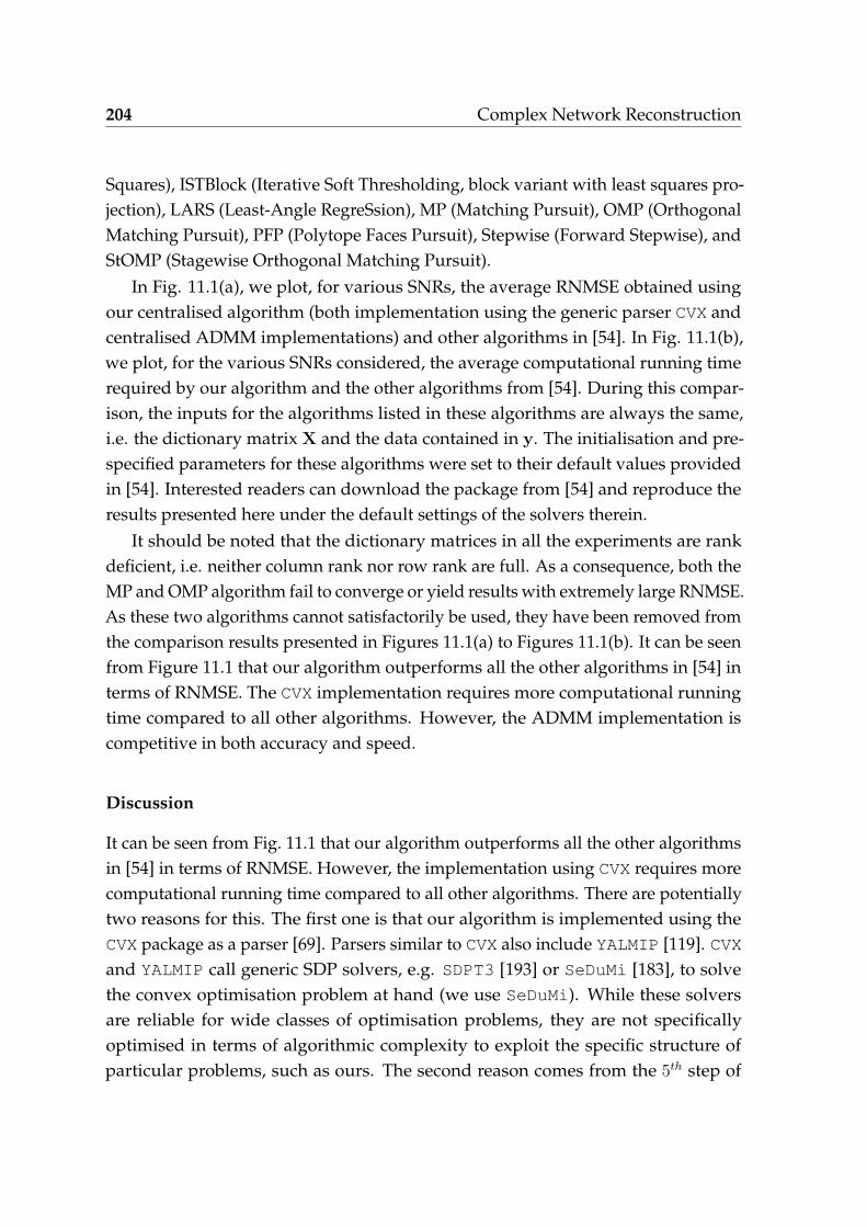
204 Complex Network Reconstruction
Squares), ISTBlock (Iterative Soft Thresholding, block variant with least squares pro-jection), LARS (Least-Angle RegreSsion), MP (Matching Pursuit), OMP (OrthogonalMatching Pursuit), PFP (Polytope Faces Pursuit), Stepwise (Forward Stepwise), andStOMP (Stagewise Orthogonal Matching Pursuit).
In Fig. 11.1(a), we plot, for various SNRs, the average RNMSE obtained usingour centralised algorithm (both implementation using the generic parser CVX andcentralised ADMM implementations) and other algorithms in [54]. In Fig. 11.1(b),we plot, for the various SNRs considered, the average computational running timerequired by our algorithm and the other algorithms from [54]. During this compar-ison, the inputs for the algorithms listed in these algorithms are always the same,i.e. the dictionary matrix X and the data contained in y. The initialisation and pre-specified parameters for these algorithms were set to their default values providedin [54]. Interested readers can download the package from [54] and reproduce theresults presented here under the default settings of the solvers therein.
It should be noted that the dictionary matrices in all the experiments are rankdeficient, i.e. neither column rank nor row rank are full. As a consequence, both theMP and OMP algorithm fail to converge or yield results with extremely large RNMSE.As these two algorithms cannot satisfactorily be used, they have been removed fromthe comparison results presented in Figures 11.1(a) to Figures 11.1(b). It can be seenfrom Figure 11.1 that our algorithm outperforms all the other algorithms in [54] interms of RNMSE. The CVX implementation requires more computational runningtime compared to all other algorithms. However, the ADMM implementation iscompetitive in both accuracy and speed.
Discussion
It can be seen from Fig. 11.1 that our algorithm outperforms all the other algorithmsin [54] in terms of RNMSE. However, the implementation using CVX requires morecomputational running time compared to all other algorithms. There are potentiallytwo reasons for this. The first one is that our algorithm is implemented using theCVX package as a parser [69]. Parsers similar to CVX also include YALMIP [119]. CVXand YALMIP call generic SDP solvers, e.g. SDPT3 [193] or SeDuMi [183], to solvethe convex optimisation problem at hand (we use SeDuMi). While these solversare reliable for wide classes of optimisation problems, they are not specificallyoptimised in terms of algorithmic complexity to exploit the specific structure ofparticular problems, such as ours. The second reason comes from the 5th step of

11.1 Centralised Identification 205
5 10 15 20 2510
−2
10−1
100
101
RNMSE Comparision For Different Algorihtms
SNR (dB)
RN
MS
E
ADMM ImplmentationCVX ImplementationBPIRWLSISTBlockLARSPFPStepwiseStOMP
(a) Parameter RNMSE ∥βestimate − βtrue∥2/∥βtrue∥2 over various SNRs.
5 10 15 20 2510
−2
10−1
100
101
102
Computational Running Time Comparision For Different Algorihtms
SNR (dB)
Com
puta
tiona
l run
ning
tim
e
ADMM ImplmentationCVX ImplementationBPIRWLSISTBlockLARSPFPStepwiseStOMP
(b) Computational running time (in seconds) over various SNRs.
Fig. 11.1 Parameter RNMSE ∥βestimate − βtrue∥2/∥βtrue∥2 and computational runningtime averaged over 200 independent experiments for the signal-to-noise ratios 0 dB,5 dB, 10 dB, 15 dB, 20 dB, and 25 dB.

206 Complex Network Reconstruction
Algorithm 4 where the M × N matrix σ2I + XU(k)W(k)X⊤ has to be inverted toupdate the weights for the next iteration. Though a pruning rule has been discussed,such inversion at each iteration is inevitable compared to the algorithms consideredin [54].
11.2 Distributed Identification
For all the following examples dealt with using ADMM implementations, we set thepenalty parameter in the augmented Lagrangian ρ = 1 and the scalar regularisationparameter λ = 0.001∥XT y∥∞. We also considered termination tolerances ϵabs = 10−4
and ϵabs = 10−2 and set the ADMM iteration number to be 200 and the weightupdating iteration number to be 5 throughout all algorithms. We set the thresholdfor pruning γ to be 10−3.
Now we introduce another performance index Phase Diagram. A useful perfor-mance index is the Phase Diagram [Donoho and Stodden], which is used to illustratehow sparsity levels (defined as ρ = K/M , where K counts the number of the nonzeroelements in β) and underdeteminedness (δ = M/N ) affect the performance of analgorithm. It should be noted that the phase diagrams presented here are empirical.More on phase diagrams, including the results, will be presented later.
Next we investigate the relation between the underdeteminedness δ = M/N andthe sparsity level ρ = K/M , i.e. the phase diagram. We use the same specificationsof the dictionary matrix as above. To recap, sine functions are used as candidatefunctions to construct the dictionary vector as Xij(k) ≜ [sin(xj(k)− xi(k))] ∈ R. Weassume the natural frequencies θi to be zero for all i. Therefore, the column size of thedictionary matrix Xi equals to the dimension of the network, i.e. N = n. However,The network topology is generated differently from the centralised identification.Here, we change the nonzero entries proportion from 10% to K/N .
In Figure 11.2, show the parameter RNMSE in the noiseless case for both Algo-rithm 4 and direct Lasso reconstruction. From Figure 11.2, we can clearly find a“cliff” or “breakdown” from dark blue to light blue area. Such cliff occurs for valuesof the RNMSE around 0.5. By Lasso reconstruction we mean one single iterationof Algorithm 4. We varied the underdeteminedness δ = M/N from 0.05 to 1 withN = 1000. The dark blue area, below the cliff, indicates the region within which thealgorithm recovered the underlying model with near zero error. Above the cliff inthe coloured area, the algorithm was unable to recover the correct model. As one

11.2 Distributed Identification 207
Underdeteminedness δ = M/N, N=1000
Sp
ars
ity ρ
= K
/M
0.1 0.2 0.3 0.4 0.5 0.6 0.7 0.8 0.9 1
1
0.9
0.8
0.7
0.6
0.5
0.4
0.3
0.2
0.1 0
0.2
0.4
0.6
0.8
1
(a) Parameter RNMSE for Algorithm 4.
Underdeteminedness δ = M/N, N=1000
Spa
rsity ρ
= K
/M
0.1 0.2 0.3 0.4 0.5 0.6 0.7 0.8 0.9 1
1
0.9
0.8
0.7
0.6
0.5
0.4
0.3
0.2
0.1 0
0.2
0.4
0.6
0.8
1
(b) Parameter RNMSE for Lasso reconstruction.
Fig. 11.2 Phase diagrams for Algorithm 4 (left panel) and Lasso reconstruction (rightpanel) in the noiseless case. The number of measurements required to correctlyreconstruct the network with Algorithm 4 is significantly lower in comparison withLasso.

208 Complex Network Reconstruction
proceeds further above the cliff, the ability of the algorithm to recover the modelprogressively drops. Each colour indicates a different RNMSE over 50 realisations.Considering both subfigures in Figure 11.2, we can see that each of the phase dia-grams shows a transition from accurate model recovery to very inaccurate as theunderlying complexity of the model increases. The “breakdown” in the error levelshows where the algorithm stops recovering the correct underlying model. Notehow increased model noise drives the breakdown point lower, at sparser models.The noise level also limits the accuracy, even when the correct model type is re-covered, as the coefficients are estimated with more noise when the noise in theunderlying data increases [Donoho and Stodden]. Carrying out additional tests forvarious network sizes N (results not shown), surprisingly, we observed that thecorresponding phase diagrams remain very similar and exhibit the same trends.This implies that, if the sparsity K can be estimated based on expert knowledge,a rough estimate of the number of observations needed to guarantee an a prioridefined reconstruction performance can be chosen. In practice, K tends to be verysmall while N is usually large due to the need to a priori consider a large number ofcandidate nonlinear dictionary functions. From the phase diagrams, it also can beimplied that the more candidate functions we introduce, the more observations weneed when sparsity is fixed.
Based on the above, it is informative to revisit the comparison where N =501. The underdeterminess M/N = 450/501 ≈ 0.9 and the sparsity level K/M ≈10/450 ≈ 0.02. Regarding various SNRs, reconstruction for data with high SNRsyields better performance. This is congruent with the results presented in the phasediagrams of Figure 11.2.
Finally, it is interesting to compare the results obtained through direct Lassoreconstruction (the first iteration of Algorithm 4) and Algorithm 4. Figure 11.2validates that Algorithm 4 delivers solutions with higher sparsity level in comparisonwith Lasso reconstruction. Moreover, the number of measurements required tocorrectly identify the structure in the noiseless case is much lower for Algorithm 4in comparison with Lasso. This is a major benefit when identifying systems withlow sampling rate and low number of measurements. In the presence of noise it ishard to quantify the performance criteria for correct reconstruction, since a largernumber of models can fit the data. However, reconstructed models obtained usingAlgorithm 4 are typically sparser in comparison with models obtained using Lasso.
Next, we compare the computational time for different network sizes by dis-tributing the computations over various numbers of CPU cores. In this comparison,

11.2 Distributed Identification 209
2 4 6 8 10 12 14
101
102
103
Number of CPU cores
Ava
rage
tota
l tim
e fo
r pa
ralle
l com
puta
tion
(se
cond
s)
N = 1000N = 2000N = 3000N = 4000N = 5000N = 6000N = 7000N = 8000N = 9000N = 10000
Fig. 11.3 Average computational running time for the βt+1i update in Algorithm
4 for a fixed sparsity K = 10 when different numbers of CPU cores and differentnetwork dimensions ranging from N = 1000 to N = 10000, are considered. Unitsare in seconds.

210 Complex Network Reconstruction
we consider only sine functions as candidate functions to construct the dictionaryelement, i.e. Xij(k) ≜ [sin(xj(k) − xi(k))] ∈ R. We assume the natural frequenciesθi to be zero for all i. Therefore, the column size of the dictionary matrix Xi equalsthe dimension of the network, i.e. N = n. Here, N is ranging from 1000 to 10000and the sparsity K is fixed to 10. For each N , time-series are generated in the samemanner as above, while M is fixed at 500. In the implementation of the distributedalgorithm, we use the MATLAB command parfor and matlabpool(‘size’) toparallelise the βk-update in Algorithm 4. The parameter size is varied from 2 to 12.Experiments over the five SNRs (5 dB, 10 dB, 15 dB, 20 dB, 25 dB) are performed foreach N . From the results we found that the computation time over each SNR variedslightly (at least within the same magnitude), which is consistent with the simulationresults presented in Figure 11.1. In Figure 11.3, we show the average computationalrunning time for different number of CPU cores used and for different networkdimensions ranging from 1000 to 10000. Each point in the figure is obtained byaveraging over 5× 50 experiments for each network size.
Discussion
One of the major drawbacks of centralised algorithm is their high computationalcomplexity in comparison with other approaches. To alleviate this drawback, wehave derived a decentralised version of the algorithm, which can be distributedbetween several computational units. We illustrate the effectiveness of our decen-tralisation algorithm by distributing the computation between several computercores and consequently showed an almost a log-linear gain in computational timefor large-scale systems.
The presented algorithm has a better performance in terms of Normalised MeanSquare Error in comparison with state-of-the-art-methods including Lasso andreweighed ℓ1 methods with a logarithmic penalty function [32]. Moreover, weempirically show that the number of observations required to obtain a correctreconstruction in the noiseless case using the presented algorithm is much lowerthan that of the standard Lasso algorithm. In the presence of noise, such an empiricalcomparison is hard to perform due to the identifiability problem. That is, we canobtain several models fitting the data with the same sparsity level but completelydifferent sparsity patterns. Hence finding a model matching the “true” structure cansimply be impossible.
Phase diagrams can provide additional insight into regression problems andthe algorithms used to solve them. In [6], the authors use dictionary matrices with

11.2 Distributed Identification 211
Gaussian i.i.d. entries and provide the first rigorous analysis that explains whyphase transitions are ubiquitous in random ℓ1 regression problems. In our setting,entries of dictionary matrices are not Gaussian i.i.d, hence the theoretical resultsfrom [6] do not apply. However, we observed that the phase diagrams for variousnetwork size N remain very similar and exhibit the same trends and “breakdowns”.Taking into account the results presented in [6], the similarities that we observedamong the phase diagrams might be more than just empirical observations. Thiswill constitute the basis for one of our future work directions.


Chapter 12
Fault Diagnosis of Power System

214 Fault Diagnosis of Power System
12.1 Introduction
Power networks are large-scale spatially distributed systems. Being critical in-frastructures, they possess strict safety and reliability constraints. The design ofmonitoring schemes to diagnose anomalies caused by unpredicted or sudden faultson power networks is thus of great importance [170]. To be consistent with theinternational definition of the fault diagnosis problem, the recommendations of theIFAC Technical Committee SAFEPROCESS is accordingly employed in what follows.Namely, this work proposes a method to: 1) decide whether there is an occurrence ofa fault and the time of this occurrence (i.e. detection), 2) establish the location of thedetected fault (i.e. isolation), and 3) determine the size and time-varying behaviourof the detected fault (i.e. identification).
Since power networks are typically large-scale and have nonlinear dynamics,fault diagnosis over transmission lines can be a very challenging problem. Thischapter draws inspiration from the fields of signal processing and machine learningto combine compressive sensing and variational Bayesian inference techniques so asto offer an efficient method for fault diagnosis.
Most of the literature available on fault diagnosis focuses on systems approxi-mated by linear dynamics [49] Beyond linear systems descriptions, the dynamics ofbuses in power networks can be described by the so-called swing equations wherethe active power flows are nonlinear functions of the phase angles. Works that haveconsidered fault detection and isolation in power networks include [171, 230, 125].[171] focuses on distributed fault detection and isolation using linearised swing dy-namics and the faults are considered to be additive. The method developed in [230]is used to to detect sensor faults assuming that such faults appear as biased faultsadded to the measurement equation. In [125], a fault detection and isolation residualgenerator is presented for nonlinear systems with additive faults. The nonlinearitiesin [125] are not imposed a priori on the model structure but treated as disturbanceswith some known patterns.
To summarise, the works [49, 171] use linear systems to characterise the dynam-ics of power networks and the faults are assumed to be additive. Though the systemdynamics are nonlinear in [230, 125], the faults are still assumed to be additive. Themethods developed on the basis of these conservative assumptions yield severalproblems. Firstly, the linear approximation to nonlinear swing equations can onlybe used when the phase angles are close to each other. However, when the system isstrained and faults appear, phase angles can often be far apart. Therefore, a linear

12.2 Power System Model 215
approximation is inappropriate in strained power network situations. Secondly, itis well-known that a large portion of power system faults occurring in transmis-sion lines do not involve additive faults, e.g. a short-circuit fault occurring on thetransmission lines between generators would correspond to some changes in the pa-rameters of the nonlinear terms appearing in the swing equation [109]. Furthermore,the inevitable and frequent introduction of new components in a power networkcontributes to the vulnerability of transmission lines, which, if not appropriatelycontrolled, can lead to cascading failures [84]. Such cascading failures cannot becaptured by additive faults. Finally, the methods mentioned above only address faultdetection and isolation rather than identification, which is crucial to take appropriateactions when faults occur on transmission lines.
Contributions. The power networks considered in this chapter are described bythe nonlinear swing equations with additive process noise. The faults are assumed tooccur on the transmission lines of the power network. The problem of fault diagnosis,i.e. detection, isolation and identification, of such nonlinear power networks isformulated as a compressive sensing or sparse signal recovery problem. To solvethis problem we consider a sparse Bayesian formulation of the fault identificationproblem, which is then casted as a nonconvex optimisation problem. Finally, theproblem is relaxed into a convex problem and solved efficiently using an iterativereweighted ℓ1-minimisation algorithm. The resulting efficiency of the proposedmethod enables real-time detection of faults in large-scale networks.
The outline of this application is as follows. Section 12.2 introduces the nonlinearmodel of power networks considered in this chapter. Section 12.3 formulates thefault diagnosis problem of power networks as a compressive sensing or sparse signalrecovery problem. Section 12.4 applies the method to a power network with 20 busesand 80 transmission lines and, finally, Section 12.5 concludes and discusses severalfuture problems.
12.2 Power System Model
Power systems are examples of complex systems in which generators and loads aredynamically interconnected. Hence, they can be seen as networked systems, whereeach bus is a node in the network. We assume that all the buses in the network areconnected to synchronous machines (motors or generators). The nonlinear modelfor the active power flow in a transmission line connected between bus i and bus j
is given as follows. For i = 1, . . . , n, the behaviour of bus/node i can be represented

216 Fault Diagnosis of Power System
by the swing equation [171, 230, 109]
miδi(t) + diδi(t)− Pmi(t) = −∑
j∈Ni
Pij(t), (12.1)
where δi is the phase angle of bus i, mi and di are the inertia and damping coefficientsof the motors and generators, respectively, Pmi is the mechanical input power, Pij
is the active power flow from bus i to j, and Ni is the neighbourhood set of bus i
where bus j and i share a transmission line or communication link.
Considering that there are no power losses nor ground admittances, and lettingVi = |Vi|ejδi be the complex voltage of bus i where j represents the imaginary unit,the active power flow between bus i and bus j, Pij , is given by:
Pij(t) = w(1)ij cos(δi(t)− δj(t)) + w
(2)ij sin(δi(t)− δj(t)), (12.2)
where w(1)ij = |Vi||Vj|Gij and Gij is the branch conductance between bus i and bus j;
and w(2)ij = |Vi||Vj|Bij and Bij is the branch susceptance between bus i and bus j.
If we let ξi(t) = δi(t) and ζi(t) = δi(t), each bus can be assumed to have doubleintegrator dynamics. The dynamics of bus i can thus be written:
ξi(t) = ζi(t), (12.3)
ζi(t) = ui(t) + vi(t), (12.4)
where ξi, ζi are scalar states, vi(t) is a known scalar external input, and ui is thepower flow
vi(t) = Pmi(t)mi
(12.5)
ui(t) = − di
mi
ζi(t)−1
mi
∑j∈Ni
[w(1)ij cos(ξi(t)− ξj(t)) + w
(2)ij sin(ξi(t)− ξj(t))]. (12.6)
The variables ξi and ζi can be interpreted as phase and frequency in the context ofpower networks.
In [171], the cos(·) terms are neglected (no branch conductance between buses)and it is assumed that phase angles are close to each other. The dynamics in (12.1)are then linearised to yield
miδi(t) + diδi(t)− Pmi(t) = −∑
j∈Ni
w(2)ij (δi(t)− δj(t)). (12.7)

12.2 Power System Model 217
Each bus i is assumed to have double integrator dynamics as described in (12.3) and(12.4). ui(t) in (12.6) becomes a linear equation
ui(t) = − di
mi
ξi(t)−1
mi
∑j∈Ni
w(2)ij (ξi(t)− ξj(t)). (12.8)
For the linearised system (12.8), a bus k is faulty if for some functions fξk(t) andfζk(t) not identical to zero either ξi(t) = ζi(t) + fξk(t), or ζi(t) = ui(t) + vi(t) + fζk(t).The functions fξk(t) and fζk(t) are referred to as fault signals. Model-based orobserver-based fault diagnosis methods are available for power networks (see [171]and reference therein). However, specific aspects need careful consideration whendealing with fault diagnosis in power networks. Firstly, the simplified linear modelcan only be used when the phase angles are close to each other. However, when thesystem is strained and faults appear, phase angles can often be far apart.
In transmission systems the sin(·) term in (12.2) is the dominating one. To performa linearisation, one often assumes “small angle differences” between nodes andhence “small” power flows. This typically works well under normal operation.However, if the power system is under a lot of strain, i.e. if power flows are closerto the theoretical maximum, the angle difference becomes close to 90 degrees andthe nonlinearity of the sin(·) term becomes quite noticeable. In particular, if, in atransient state, the angle difference exceeds 90 degrees, generators typically loosesynchrony and trip. This is not captured by linear models. In such circumstances, thelinear model cannot be used to approximate the nonlinear model in (12.1) anymore.Secondly, power networks are highly distributed and interconnected, and more thanone transmission line can be faulty at a given time. Thirdly, to be more realistic,some process noise εi should be incorporated into the second-order system (12.1) foreach bus i:
miδi(t) + diδi(t)− Pmi(t) = −n∑
j=1Pij(t) + εi(t), (12.9)
Based on the swing equation above, the state space model (12.3) and (12.4) can thenbe rewritten under the form:
ξi(t) = ζi(t), (12.10)
ζi(t) = ui(t) + vi(t) + εi(t), (12.11)

218 Fault Diagnosis of Power System
where the noise εi(t) is assumed to be i.i.d. Gaussian with
E(εi(p)) = 0E(εi(p)εi(q)) = ϵ2
i δ(p− q).
Remark 23 Here we only consider a dynamical system model with process noise εi since, inpower networks, the measurement noise is small and would typically not have a catastrophiceffect on the performance of detection algorithms [187].
12.3 Fault Diagnosis Problem of Nonlinear Power Sys-tems
Given the model and explanation above, we primarily focus on the following settingin this chapter.
Definition 5 If a power network can be described by (12.10) and (12.11), the transmissionline between bus i and bus j is f
¯aulty when w
(1)ij changes to a new scalar w
[f ](1)ij and/or w
(2)ij
changes to a new scalar w[f ](2)ij , where w
(1)ij and w
(2)ij are the weights for the cos and sin terms
defined in (12.6).
Based on the considerations above and Definition 5, the problem that we are inter-ested in solving is the following:
Problem 11 Having access to the measurements and the distribution of the noise, howcan we detect the occurrence and magnitude of a fault, namely, how can we estimate themagnitude of the errors w
(1)ij − w
[f ](1)ij and w
(2)ij − w
[f ](2)ij , ∀i, j, using the smallest possible
number of samples.
In what follows we make the following assumption.
Assumption 11 The power networks described by (12.10) and (12.11) are fully measurable,i.e. the phase angles of all the buses can be measured.
12.3.1 Model Transformation
Applying the forward Euler discretisation scheme to (12.10) and (12.11) and as-suming the discretisation step ∆t is constant for all k, we obtain the following

12.3 Fault Diagnosis Problem of Nonlinear Power Systems 219
discrete-time system approximation to the continuous-time system (12.10) and(12.11):
ξi(t + 1)− ξi(t)∆t
= ζi(t), (12.12)
ζi(t + 1)− ζi(t)∆t
= ui(t) + vi(t) + ηi(t), (12.13)
where the noise ηi(tk) is assumed to be i.i.d. Gaussian distributed: ηi(tk) ∼ N (0, σ2i ),
with E(ηi(tp)) = 0, E(ηi(tp)ηi(tq)) = σ2i δ(tp − tq).
Defining the new variable
ei(t + 1) ≜ −(ζi(t + 1)− ζi(t))∆t
− diζi(t)mi
+ Pmi(t)mi
, (12.14)
we have
ei(t + 1) = 1mi
∑j∈Ni
[w(1)ij cos(ξi(t)− ξj(t)) + w
(2)ij sin(ξi(t)− ξj(t))] + ηi(t), (12.15)
where ei, the power flow measurement, is treated as the output of the system. Sincethe state variables ζ(t + 1) and ζ(t), the parameters ∆t, di and mi, and the input Pmi
are known, the quantity ei(t + 1) can be computed in real time. It should be notedthat “real time” is to be understood as “within the sampling time ∆t of the sensorsin power generators”.
By defining x(t) = [ξ1(t), . . . , ξN(t)] we can write (12.14) into a vector form:
ei(t + 1) = fi(x(t))βtruei + ηi(t), (12.16)
withfi(x(t)) = [f (1)
i (x(t)), f(2)i (x(t))] ∈ R2n,
f(1)i (x(t)) = [cos(ξi(t)− ξ1(t)), . . . , cos(ξi(t)− ξN(t))] ∈ Rn,
f(2)i (x(t)) = [sin(ξi(t)− ξ1(t)), . . . , sin(ξi(t)− ξN(t))] ∈ Rn,
βtruei = [β(1)
i , β(2)i ]T ∈ R2n,
β(1)i = [w(1)
i1 , . . . , w(1)iN ] ∈ Rn,
β(2)i = [w(2)
i1 , . . . , w(2)iN ] ∈ Rn,
where fi(x(t)) represents the transmission functions and βi represents the corre-sponding transmission weights associated to the topology of the network.

220 Fault Diagnosis of Power System
Remark 24 In real power systems, a sampling frequency for phasor measurement unit(PMU) as high as 2500 samples per second can be achieved. In this case, the sampling time∆t is 4 ∗ 10−5 second and the Euler discretisation ξi(t+1)−ξi(t)
∆twill typically provide a good
approximation of ξi(t).
12.3.2 Fault Diagnosis Algorithm
As stated in Definition 5, if there are no faults occurring in the transmission linesbetween bus i and other buses, the dynamics of the power networks will evolveaccording to (12.16). The e
¯xpected output for the next sampling time is defined to be
e[e]i (t + 1) = fi(x(t))βtrue
i . (12.17)
From (12.16) and (12.17), it is easy to show that ei(t + 1)−e[e]i (t + 1) is a stochastic vari-
able with zero mean and variance σ2. If there are faults occurring in the transmissionlines between bus i and other buses, the corresponding transmission weights willchange from βtrue
i to βfaulti . Similar to the definition of βtrue
i , βfaulti = [β[f ](1)
i , β[f ](2)i ]T
where β[f ](1)i = [w[f ](1)
i1 , . . . , w[f ](1)iN ] and β
[f ](2)i = [w[f ](2)
i1 , . . . , w[f ](2)iN ]. We thus have:
e[f ]i (t + 1) = fi(x(t))βfault
i + ηi(t), (12.18)
where e[f ]i is the output when there are f
¯aults.
From (12.17) and (12.18), it is easy to find that e[f ]i (t + 1)−e
[e]i (t + 1) is a stochastic
variable with mean fi(x(t))(βfaulti − βtrue
i ) and variance σ2. Denoting
yi = e[f ]i − e
[e]i , βi = βfault
i − βtruei ,
we have:yi(t + 1) = fi(x(t))βi + ηi(t). (12.19)
Remark 25 We formulate the faults identification problem as a linear regression problem.The dependent variable e
[f ]i (t + 1)− e
[e]i (t + 1) is the difference between the expected output
and the faulty output; the unknown variable we want to estimate is the difference betweenthe faulty transmission weights and the true transmission weights.
There are three problems of interest based on the formulation in (12.19): a) detectionof a fault; b) isolation of a fault, i.e. determination of the type, location and time of

12.3 Fault Diagnosis Problem of Nonlinear Power Systems 221
occurrence of a fault; and c) identification of the size and time-varying behaviour ofa fault. In the noiseless case, when there are no faults, ∀i, yi and βi are both equalto zero. On the other hand, when there are faults, certain yi are nonzero. So thefaults can be detected by identifying the entries yi that are nonzero. However, in thenoisy case, even when there are no faults, yi is nonzero most of the time since it is astochastic variable with zero mean. This can be interpreted in a probabilistic way byChebyshev’s Inequality:
p(|ei(t + 1)− e[e]i (t + 1)| ≥ lσ = σ∗) ≤ 1
l2
where l ∈ R+. According to this inequality, when there are no faults, the deviationbetween true and expected outputs, i.e. |ei(t + 1) − e
[e]i (t + 1)| cannot be much
greater than zero with high probability. On the other hand, when there is a fault, thedeviation between faulty and expected outputs, i.e. |e[f ]
i (t + 1)− e[e]i (t + 1)| should
be much greater than zero with high probability.
From an isolation point of view and Chebyshev’s inequality, when |e[f ]i (t + 1)−
e[e]i (t + 1)| is much greater than σ, the fault can be isolated with high probability (e.g.
if the threshold is set to lσ = 10σ, then the probability is 99%).
If at time t0 faults have been detected and isolated, the remaining task is toperform fault identification, i.e. to identify the location of the faults or equivalently tofind the nonzero entries in wi. Assuming that M +1 successive data points, includingthe initial data point at t0, are sampled and defining N = 2n and
yi ≜ [yi(t1), . . . , yi(tM)]T ∈ RM ,
Xi ≜
f
(1)i (x(t0)) f
(2)i (x(t0))
......
f(1)i (x(tM−1)) f
(2)i (x(tM−1))
=
fi(x(t0))
...fi(x(tM−1))
∈ RM×N ,
ηi ≜ [ηi(t0), . . . , ηi(tM−1)]T ∈ RM ,
(12.20)
we can write N independent equations of the form:
yi = Xiβi + ηi, (i = 1, . . . , n). (12.21)

222 Fault Diagnosis of Power System
Based on the formulation in (12.21), our goal is to find βi given the output datastored in yi.
To solve for βi in (12.21) amounts to solving a linear regression problem. Thiscan can be done using standard least square approaches. It should be noted thatthe linear regression problem for bus i in (12.21) is independent from the the linearregression problems for the other buses. In what follows, we will focus on findingthe solution to one of these linear regression problem and omit the subscripts i in(12.21) for simplicity of notation. We thus write
y = Xβ + η, (12.22)
where y is the difference between the faulty measurements and the expected mea-surements, or namely, the error measurements; and β is the difference between thefaulty parameters and the true parameters, or namely, the faults. We address thislinear regression problem under the following assumption.
Assumption 12 A maximum of S transmission lines are faulty, i.e. β has at most S
non-zero entries. In other words, β is S-sparse or mathematically, ∥w∥0 ≤ S. The constantS is assumed unknown to the system administrator.
Remark 26 Assumption 12 is realistic for small values of S since in the context of a powersystem, it is typically not the case that all the transmission lines are faulty simultaneously.Furthermore, since buses in power networks are typically sparsely connected the numberof faults is typically much smaller than the size of the network n, i.e. S ≪ n. ThereforeS ≪ N = 2n.
On the other-hand, the size of y equals to the number of samples needed toidentify the location of the faults after the they occur. From a practical viewpoint, thenumber of samples should be as small as possible. However, standard least squareapproaches to (12.22) cannot meet this goal as they require at least 2N samples.Moreover, the solution to the standard least square problem is generically dense(hence, violating Assumption 12) and cannot be used to identify which transmissionlines are likely to be faulty by identification of the nonzero entries of the estimatedβfault − βtrue.
Based on Algorithm 19, we can summarise the fault diagnosis algorithm fornonlinear power systems in Algorithm 20.

12.3 Fault Diagnosis Problem of Nonlinear Power Systems 223
Algorithm 20 Diagnosis for faults
1: Set a threshold σ∗ as indicated in Section 12.3.2, e.g. σ∗ = 10× σ;2: for k = 0, . . . , T do3: % T is an integer indicating the number of diagnosis rounds;4: Collect ξi(t) and ζi(t) in (12.12) and (12.13)5: for i = 1, . . . , N do6: Calculate the output data ei(t + 1) in (12.14);7: Calculate the expected output e
[e]i (t + 1) in (12.17);
8: if |ei(t + 1)− e[e+]i (t + 1)| > σ∗ then
9: Fault is detected for bus i; % {fault detection procedure}10: Compute yi(t + 1) in (12.19);11: if |yi(t + 1)| > σ∗ then12: Isolate bus i; % {fault isolation procedure}13: end if14: end if15: Set M ← k;16: Apply Algorithms propose in Chapter 6.6 to identify the faults βi; % {fault
identification procedure}17: end for18: if ∀i, ∥βi∥0 converge to some constant then19: Break;20: end if21: end for22: An estimate for the faults β in (12.21), i = 1, . . . , n.

224 Fault Diagnosis of Power System
12.4 Numerical Study
The effectiveness of our theoretic developments is here illustrated for a randomlygenerated power network with 20 buses. If all the buses are fully connected, thepossible number of transmission lines is 380. We assume that the number of trans-mission lines is 79 (i.e. we assume that the sparsity of the network is around 20%).Its dynamics can be described by the nonlinear swing equations described in (12.10)and (12.11). w
(1)ij and w
(2)ij are positive real numbers as shown in Fig. 12.3(a). Let the
noise variance σ2 = 1. All the parameter values are selected to be similar to those in[109, 146].
Since the sampling frequency is around 50 Hz for the PMU [109, 146], we assumethe sampling interval to be 20 ms. We thus assume that the discretisation step inSection 12.3 is performed using a sampling interval ∆t = 20 ms.
Consider the power networks model in (12.10) and (12.11). At time instant t = 3s,there are faults occurring in five transmission lines simultaneously. Specifically, arandomly chosen set of faults can be described as follows:
∀(i, j) ∈ {(5, 18), (7, 2), (11, 15), (16, 18), (19, 9)}
, w(1)ij and w
(2)ij in (12.6) respectively (which correspond to cos and sin terms) are set
to zeros. 5 buses are involved in these transmission lines, i.e. buses 5, 7, 11, 16 and19. Following the procedure in Algorithm 20, we want to detect and isolate these 5buses. After detection and isolation, the identification procedure will be performed.We consider σ∗ = 10σ = 10 to initialise Algorithm 20.
First, we detect and isolate the buses with |yi(t + 1)| > σ∗. In Fig. 12.1, it can beseen that at time instant t = 3.02s (only one sampling time after the faults occur), |y5|,|y7|, |y11|, |y16| and |y19| are much greater than σ∗ (we set σ∗ = 10 here). Therefore,we can draw the conclusion that buses 5, 7, 11, 16 and 19 are faulty and should beisolated. Next, we identify the faults that occur in the transmission lines connectingthe previously isolated buses, i.e. buses 5, 7, 11, 16 and 19. In Fig. 12.2, the timetrajectory of the sparsity of the estimated fault ∥βi∥0, i.e. ∥βfault
i −βtruei ∥0 (see Remark
25), for i = 5, 7, 11, 16, 19 are depicted starting at the time point t = 3.02s when thefaults are detected. We set the pruning threshold to 10−3 during the identificationprocedure of the faults. We define a positive integer n∗ to indicate the number ofidentification rounds which are required to terminate the identification procedure,e.g. n∗ = 10. As shown in Fig. 12.2, at time instant t = 3.52s, the sparsity of the

12.5 Conclusion and Discussion 225
0 1 2 3 4 5 6−40
−30
−20
−10
0
10
20
30
40
Time (s)
yi
bus 5bus 7bus 11bus 16bus 19
Fig. 12.1 Time-series of yi for all buses. The black dashed lines indicate the thresholdσ∗ in Algorithm 20. The coloured solid lines are the phase angle measurements forbus i, i = 5, 7, 11, 16, 19. At time instant t = 3.02s, |y5|, |y7|, |y11|, |y16| and |y19| aremuch greater than σ∗ (σ∗ = 10 here).
estimated fault, i.e. ∥wfaulti −wtrue
i ∥0 for bus i = 5, 7, 11, 16, 19 all become equal to 2and remain unchanged afterwards. At time instant t = 3.72s, only n∗ = 10 samplingrounds after t = 3.52s, we terminate the identification procedure as the sparsity forall the estimated faults is considered to be stable.
In Fig. 12.3(a) and Fig. 12.3(b), we illustrate the true weight matrix and theestimated absolute error matrix |βfault
i − βtruei |. As we can see, all the 5 faults that are
occurring in the transmission lines have been identified with high accuracy.
12.5 Conclusion and Discussion
In this Chapter, we addressed the problem of automatic fault diagnosis in large-scale power networks where the buses are described by second-order nonlinearswing equations with process noise. In particular, this work focused on a classof transmission lines faults. We combined tools from compressive sensing andvariational Bayesian inference to develop a method to detect, isolate and identify

226 Fault Diagnosis of Power System
3 3.1 3.2 3.3 3.4 3.5 3.6 3.7 3.8 3.9 40
0.5
1
1.5
2
2.5
3
3.5
4
Time (s)
Theestimated‖w
fau
lti
−w
true
i‖ 0
bus 5bus 7bus 11bus 16bus 19
Fig. 12.2 Time-series of the sparsity of the estimated fault, i.e. ∥wfaulti −wtrue
i ∥0 forbus i = 5, 7, 11, 16, 19.
the faults. An illustrative example showed the application of the proposed methodto fault diagnosis in nonlinear power networks.
Beyond the results in this chapter, some issues still remain for further investiga-tion. This chapter assumed that the system is fully measurable. Current work aimsto extend the proposed framework to fault diagnosis with partially measured powersystems.

12.5 Conclusion and Discussion 227
5 10 15 20 25 30 35 40
5
10
15
2010
20
30
40
50
60
70
80
90
(a) True weight matrix
5 10 15 20 25 30 35 40
5
10
15
20
5
10
15
20
25
30
35
(b) Absolute error weight matrix: |βfaulti − βtrue
i | (see Remark 25)
Fig. 12.3 Identification of transmission lines faults: (a) describes the true weightmatrix with around 20% nonzero entries. The left half of the matrix correspondsto the weights for cos(·) terms while the right half is for sin(·) terms. (b) representsthe absolute error weight matrix, which is defined as |βfault
i − βtruei |. The non-
zero terms in the heat map correspond directly to the faulty transmission lines:(5,18),(7,2),(11,15),(16,18),(19,9).


Part IV
Conclusion and Future Direction


Chapter 13
Conclusion

232 Conclusion
In summary, this thesis makes some attempts to address the following challengesarising in big time series data analytics
General Problem Formulation for Nonlinear System Identification: Modern timeseries data are often ultra-high dimensional (e.g. biology data, power systems data).Furthermore, the type of data used for modelling are collected in different fashions,e.g., from single or heterogeneous sources; collected “statically” or “streamingly”.The underlying dynamical systems are often large-scale (e.g. gene networks, powernetworks). However, the representation of nonlinear dynamical systems is extremelysimple or sparse. This thesis adapts and extends the regularised sparse learningformulation in different aspects to address various nonlinear identification problems.
Both a selection of time-invariant and time-varying nonlinear dynamical systemsare covered. For time-invariant system, the classic nonlinear system identificationproblem from single dataset is addressed in the beginning. Then we move to a morepractical and significant yet complicated scenario where heterogeneous datasets areused simultaneously. Such datasets typically contain (a) data from several replicatesof an experiment performed on a biological system of interest and/or (b) datameasured from a biochemical system subjected to different experimental conditions,for example, changes/perturbations in biological inductions, temperature, geneknock-out, gene over-expression, etc. For time-varying systems, the regime-switchsystem identification problem is considered, i.e., the problem of identifying boththe switching points and the nonlinear model structure within each regime. Thenthe abrupt change point detection problem is considered. Using these, the classictrending filtering and fault diagnosis problems are revisited. All the identificationproblems are formulated as various ℓ0 type optimisation problems. In the end, wediscuss some technical issues on data processing arising from practical applications.
Efficient Nonlinear System Identification Algorithms: These algorithms are notdistinct and can be formulated in a unified way using Bayesian Learning with struc-tural sparse prior. Furthermore, we suggest a series of iterative reweighted convexrelaxation schemes for connecting these algorithms to popular algorithms includingLasso, Group-Lasso, Generalised-Lasso, Fused-Lasso and Graphical-Lasso. In thispart, we go beyond from simple nonlinear model class to more general class; fromdata likelihood in Gaussian distribution to the more general exponential family. Theestimation of the stochastic term also discussed including ARMA and ARCH. Manyoptimisation framework, such as (stochastic) gradient descent, Newton method,

233
Quasi-Newton method, alternating direction method of multiplier can be seamlesslyintegrated into our formulation as either centralised or distributed optimisationstrategy to address high dimensionality and large scale problems. These algorithmslargely enrich not only the family of time series modelling algorithms but also sparsesignal recovery/modelling/estimation algorithms in various communities.
Future Directions Two future research directions based on the output of this thesisare pointed out, both related to “neurons”. The first is focusing on theory andalgorithm about modelling/identification/learning on deep neural networks. Thesecond is focusing applications in neuroscience: understanding the neural basis ofdecision making using mathematical modelling from big data. Some promisingresults have showed the feasibility and potential impact of these directions.


Chapter 14
Future Direction

236 Future Direction
In this Chapter, several future works will be discussed. The begin with, I willdiscuss the possibility to the linear system identification problem. Fortunately, twopapers are published on the internet in which I was co-authored and initialised theidea, see Yue et al. [225], Jin et al. [96]. However, I will not include them in my thesisas a contribution of mine.
Recently, deep learning using deep neural network representation has beensuccessfully applied in many artificial intelligence applications. Interestingly, learn-ing/modelling/identifying a (deep) neural network is essentially a Nonlinear SystemIdentification problem as introduced by Lennart Ljung in [117, pp. 154] twenty yearsago. Maybe due to some historical reason, neural networks in Lennart Ljung’sbook [117] has not been discussed a lot, only 2 pages contents are about neuralnetwork in his 609 pages book, say, multi-layer networks and recurrent neural net-work. Now in this thesis, it is probably a good time to discuss more on learning(identification) of deep neural networks from the perspective of nonlinear systemidentification. Some promising results have showed the feasibility and potentialimpact of the proposed directions.
It seems that the mechanism of human brain governing intelligence inspiredgreatly the research in deep learning. Vice versa, to understand how brain works isprominent and been hot for decades. In particular, the decision making process inhuman is of great interest for myself. Given the incredible amount of neural data,such as EEG, ECG, fMRI, etc., all recorded in terms of time series, there is greatpotential to model the brain network to understand the mechanism.
14.1 Future Direction I: Bayesian Deep Learning
14.1.1 Background on Deep Learning and Deep Neural Networks
It is commonly accepted for a deep learning system, the underlying neural network(NN) has to be big and complex. We argue that this perception may not be true.Many of the neurons and their associated connections, both incoming and outgoingones, can be dropped permanently which results in a NN with much smaller size. Thisis very similar to sparse distributed representations in brain. The human neocortexhas roughly 100 billion neurons, but at any given time only a small percent areactive in performing a particular cognitive function [130]. For the non-sequenceor non time dependent data, the active neurons may be fixed and not change overtime [43]. Dropping neurons is also the key idea in Dropout [86, 180], a successful

14.1 Future Direction I: Bayesian Deep Learning 237
regularisation technique to prevent overfitting in NNs. In their work, the neuronsare dropped temporarily in training. In the end for prediction, the model is still of fullsize and fully connected.
Hereafter, we aim at training a simple network when it can achieve comparableperformance to the fully connected NN, but with number of neurons and connectionsas few as possible. Dropping connections may be not difficult by introducing weightdecay regularisers. However, dropping neurons is challenging. On one hand, theweight decay regularisation can’t penalise all the connections associated with oneneuron simultaneously. On the other hand, it is attempted to suppress the neurons tofire such as the use of rectifier as activation function [66], regularisation techniqueslike K-L sparsity in the sparse autoencoder variants [103, 20], or constraints likemax-norm [178, 67]. However, a neuron not firing in training still can’t be droppedfor testing and prediction since her connections’ weights are not zeros. As analternative, network pruning by dropping connections below a threshold has beenwidely studied to compress a pre-trained fully connected NN models reduce thenetwork complexity and over-fitting, see early work [111, 78] and more recently[75, 74]. Unfortunately, such pruning strategy may not effectively drop neurons.For example, a NN may consist of large number of neurons but few connections.Though, the model size/storage space may not be challenging but bring anotherchallenge for chip design for storage and computation, e.g. (mobile) GPU, FPGA,etc.
We use the following notation throughout this Chapter. Bold lower case letters(x) denote vectors, bold upper case letters (X) denote matrices, and standard weightletters (x) denote scalar quantities. We use subscripts to denote variables as well Wℓ
(such as W1 : n0 × n1, W2 : n1 × n2). n0 is the number of features of the input. Weuse subscripts to denote either entire rows (Wℓ
p,: for the p-th row of Wℓ) or entirecolumns (Wℓ
:,q for the q-th column of Wℓ). We use the standard capital letter withsubscript to denote the element index of a specific variable: W 1
p,q denotes the elementat row p column q of the variable W1. We also use Oℓ to be the indicator for theneurons in layer ℓ. For example, O0 consist of n0 neurons in the input layer, indexedas O0
1, . . . , O0n0 .
We start with the case of a three layer NN with a single hidden layer. The generali-sation to multiple layers is straightforward. Denote by W1, W2 the weight matricesconnecting the first layer to the hidden layer and connecting the hidden layer tothe output layer respectively. These linearly transform the layers’ inputs beforeapplying some element-wise non-linearity σ(·). Denote by b the biases by which we

238 Future Direction
shift the input of the non-linearity. We assume the model to output n2 dimensionalvectors while its input is n0 dimensional vectors, with K hidden units. Thus W1 is an0 × n1 matrix, W2 is a n1 × n2 matrix, and b is a n1 dimensional vector. A standardNN model would output the following given some input x
y = σ(xW1 + b)W2 (14.1)
To use the NN model for regression we might use the Euclidean loss (also knownas “square loss”),
Eregression = 12N
N∑n=1||yn − yn||22 (14.2)
where {y1, . . . , yN} are N observed outputs, and {y1, . . . , yN} being the outputs ofthe model with corresponding observed inputs {x1, . . . , xN}.
To use the model for classification, predicting the probability of x being classifiedwith label 1, ..., D, we pass the output of the model y through an element-wisesoftmax function to obtain normalised scores: pnd = exp(ynd)/ (∑d′ exp(ynd′)). Takingthe log of this function results in a softmax loss,
Eclassification = − 1N
N∑n=1
log(pn,cn) (14.3)
where cn ∈ [1, 2, ..., D] is the observed class for input n.
During optimisation regularisation terms are often added. Some of the wellknown regularisation include ℓ1 regularisation and ℓ2 regularisation, defined as
l1_regulariser ≜ λℓ1
L∑ℓ=1
(∥Wℓ∥1 + ∥bℓ∥1)
l2_regulariser ≜ λℓ2
L∑ℓ=1
(∥Wℓ∥22 + ∥bℓ∥2
2)(14.4)
where λℓ1 and λℓ2 are often called weight decay or regularisation parameter whichneeds fined tuned.
Then it results in a minimisation objective (often referred to as cost),
L ≜ E + l1_regulariser or L ≜ E + l2_regulariser, (14.5)

14.1 Future Direction I: Bayesian Deep Learning 239
or a mixture of l1_regulariser and l2_regulariser, which is known as elas-tic net.
The goal of introducing l1_regulariser and l2_regulariser is to penalisethe connections’ weights between neurons to prevent overfitting. However, theapplication of such regularisers alone in deep neural network are not as successfulas in linear regression and logistic regression. On the other hand, in the hardwarecomputation especially using GPU, dropping connections may not save computationtime and memory unless some special coding and processing is used [74]. Theintroduction of dropout achieve great success to avoid over-fitting in practice [86,180] with these two regularisers. These regularisation techniques are suitable forpreventing overfitting but may not be helpful in simplifying the NN structure. Webelieve that the key to automatically simplify a NN structure in training is to defineproper regulariser by exploring the sparsity structure of the NN in a deep learningsystem.
14.1.2 Structural Sparsity in Deep Neural Network
Multi Layer Perceptron
Hereafter, we are seeking a strategy to drop neurons. Using the standard setup forNN, we have the weight matrix from layer ℓ− 1 to layer ℓ,
Wℓ =[(Wℓ
1,:)⊤, . . . , (Wℓnℓ−1,:)⊤
]⊤=[Wℓ
:,1, . . . , Wℓ:,nℓ
](14.6)
where Wℓi,: denote the i-th row of Wℓ, i = 1, . . . , nℓ−1; it encodes the incoming
connections’ weights from layer ℓ− 1 to the i-th neuron in layer ℓ, i.e., Oℓi . Similarly,
Wℓ:,j denote the j-th column of Wℓ, j = 1, . . . , nℓ; it encodes the outgoing connections’
weights of the j-th neuron in layer ℓ, i.e., Oℓi to all the neurons in the next layer, i.e.,
layer ℓ + 1 . In particular, O0i denotes the i-th feature/neuron in input layer.
We first introduce two new regularisers, the first one is called li_regulariser(λℓi)
li_regulariser ≜ λℓi
L∑ℓ=1
nℓ∑j=1∥Wℓ
:,j∥2 = λℓi
L∑ℓ=1
nℓ∑j=1
√√√√nℓ−1∑i=1
(W ℓ
ij
)2(14.7)
This is used to regularise the incoming connections’ weights of all the neurons acrossdifferent layers over the whole network. The conceptual idea of removing all theincoming weights to neuron Oℓ
1 from the neurons in layer ℓ− 1 therefore removal ofherself is illustrated by comparing in Fig. 14.1(a) and14.1(c).

240 Future Direction
Layer𝑙−1
Layer𝑙
𝑊+,-./0 𝑊+,-.1
0 𝑊+,-.+,0
𝑊/+,0𝑊//0
𝑊1/0 𝑊11
0
𝑂/03/
𝑂103/
𝑂+,-.03/
𝑂/0 𝑂10 𝑂+,0
𝑊/10
𝑊1+,0
(a) Wℓ ∈ Rnℓ−1×nℓ
from layer ℓ− 1 to layer ℓ
𝑊"#$%&$ 𝑊"#'
%&$ 𝑊"#"#()%&$
𝑊$"#()%&$𝑊$$%&$
𝑊'$%&$ 𝑊''
%&$
𝑂$%
𝑂'%
𝑂"#%
𝑂$%&$ 𝑂'%&$ 𝑂"#()%&$
𝑊$'%&$
𝑊'"#()%&$
Layer𝑙
Layer𝑙 + 1
(b) Wℓ+1 ∈ Rnℓ×nℓ+1from layer ℓ to layer
ℓ + 1
Layer𝑙−1
Layer𝑙
𝑊+,-./0 𝑊+,-.1
0 𝑊+,-.+,0
𝑊/+,0𝑊//0
𝑊1/0 𝑊11
0
𝑂/03/
𝑂103/
𝑂+,-.03/
𝑂/0 𝑂10 𝑂+,0
𝑊/10
𝑊1+,0
(c) Wℓ ∈ Rnℓ−1×nℓ
from layer ℓ− 1 to layer ℓ
𝑊"#$%&$ 𝑊"#'
%&$ 𝑊"#"#()%&$
𝑊$"#()%&$𝑊$$%&$
𝑊'$%&$ 𝑊''
%&$
𝑂$%
𝑂'%
𝑂"#%
𝑂$%&$ 𝑂'%&$ 𝑂"#()%&$
𝑊$'%&$
𝑊'"#()%&$
Layer𝑙
Layer𝑙 + 1
(d) Wℓ+1 ∈ Rnℓ×nℓ+1from layer ℓ to layer
ℓ + 1
Fig. 14.1 A graphical illustration on the strategy of removing neurons. Oℓk denotes the
k-th neuron in layer ℓ , W ℓij denotes the weight of connection from neuron i in layer
ℓ to neuron j in layer ℓ + 1. The bottom figures showed a neuron can be removedeither when all incoming connections’ weights to her or her outgoing connections’weights are zeros simultaneously.
The second one is called lo_regulariser(λℓo)
lo_regulariser ≜ λℓo
L∑ℓ=1
nℓ−1∑i=1∥Wℓ
i,:∥2 = λℓo
L∑ℓ=1
nℓ−1∑i=1
√√√√√ nℓ∑j=1
(W ℓ
ij
)2(14.8)
This is used to regularise the outgoing connections’ weights of all the neurons acrossdifferent layers over the whole network. The conceptual idea of removing all theoutgoing weights from neuron Oℓ
1 to the neurons in layer ℓ + 1 therefore removalof herself is illustrated by comparing in Fig. 14.1(b) and 14.1(d). The key idea of

14.1 Future Direction I: Bayesian Deep Learning 241
introducing the two regularisers is to embed a dropping mechanism in a deep NNtraining process. Such a dropping mechanism is guided by the two regularisers.
Convolutional Neural Network
In convolutional neural network, each filter consist of a couple of neurons, the ideais to “drop” the filter thereafter a batch of neurons simultaneously. To integrate overthe filters, we reformulate the convolution as a linear operation – an inner-productto be exact. Let Fkℓ ∈ Rh×w×Kℓ−1 for kℓ = 1, ..., Kℓ be the CNN’s filters with height h,width w, and Kℓ−1 channels in the ℓ’th layer. The input to the layer is represented asa 3 dimensional tensor x ∈ RHℓ−1×W ℓ−1×Kℓ−1 with height Hℓ−1, width W ℓ−1, and Kℓ−1
channels. Convolving the filters with the input with a given stride s is equivalentto extracting patches from the input and performing a matrix product: we extracth× w ×Kℓ−1 dimensional patches from the input with stride s and vectorise these.Collecting the vectors in the rows of a matrix we obtain a new representation for ourinput x ∈ Rn×hwKℓ−1 with n patches. The vectorised filters form the columns of theweight matrix Wℓ ∈ RhwKℓ−1×Kℓ . The convolution operation is then equivalent tothe matrix product xWℓ ∈ Rn×Kℓ . The columns of the output can be re-arranged to a3 dimensional tensor y ∈ RHℓ×W ℓ×Kℓ (since n = Hℓ ×W ℓ). Pooling can then be seenas a non-linear operation on the matrix y.
Then we introduce a new regulariser over each filter
Kℓ∑k=1∥Wℓ
:,k∥2 (14.9)
The idea can be illustrated in Figure.14.2. Then we define the following regulariserto drop filters in CNN
lcnn_regulariser ≜ λℓcnn
L∑ℓ=1
Kℓ∑k=1∥Wℓ
:,k∥2 (14.10)
Or equivalently, we regularise the tensor directly. Suppose
Fkℓ ≜[fkℓ
x,y,z
]∈ Rh×w×Kℓ−1
,

242 Future Direction
Fig. 14.2 A graphical illustration on the strategy of removing the filters in convolu-tional neural networks
we have
lcnn_regulariser ≜ λℓcnn
L∑ℓ=1
Kℓ∑kℓ=1
√√√√√ h∑x=1
w∑y=1
Kℓ−1∑z=1
(fkℓ
x,y,z
)2. (14.11)
Recurrent Neural Network
The RNN dynamics can be described using deterministic transitions from previousto current hidden states. The deterministic state transition is a function
RNN : hl−1t , hl
t−1 → hlt.
For classical RNNs, this function is given by
hlt = f(Tn,nhl−1
t + Tn,nhlt−1), where f ∈ {sigm, tanh} .
Given an input sequence x = (x1, . . . , xT ), a standard recurrent neural network(RNN) computes the hidden vector sequence h = (h1, . . . , hT ) and output vectorsequence y = (y1, . . . , yT ) by iterating the following equations from t = 1 to T :
ht = H (Wxhxt + Whhht−1 + bh) (14.12)
yt = Whyht + by (14.13)

14.1 Future Direction I: Bayesian Deep Learning 243
� ��ct
Cell
f� ��f Forget gate6
�
���hlt−1
AAK hl−1t
� ��iInput
gate
AU
hlt−1
���
hl−1t
� ��o Output
gate
AU
hlt−1
���
hl−1t
� ��g
Inputmodulation
gate
f× --
JJJ f×- -? hl
thlt−1
hl−1t��:XXz
Fig. 14.3 A graphical representation of LSTM memory cells (there are minor differ-ences in comparison to Graves [70]).
where the W terms denote weight matrices (e.g. Wxh is the input-hidden weightmatrix), the b terms denote bias vectors (e.g. bh is hidden bias vector) andH is thehidden layer function.
The LSTM has complicated dynamics that allow it to easily “memorize” infor-mation for an extended number of timesteps. The “long term” memory is stored ina vector of memory cells cl
t ∈ Rn. Although many LSTM architectures that differ intheir connectivity structure and activation functions, all LSTM architectures haveexplicit memory cells for storing information for long periods of time. The LSTMcan decide to overwrite the memory cell, retrieve it, or keep it for the next time step.The LSTM architecture used in our experiments is given by the following equationsGraves [70]:
LSTM : hl−1t , hl
t−1, clt−1 → hl
t, clt (14.14)
iℓt = sigm
(Wℓ
xihℓ−1t + Whih
ℓt−1 + Wℓ
cicℓt−1 + bℓ
i
)(14.15)
f ℓt = sigm
(Wℓ
xfhℓ−1t + Wℓ
hfhℓt−1 + Wℓ
cfcℓt−1 + bℓ
f
)(14.16)
oℓt = sigm
(Wℓ
xohℓ−1t + Wℓ
hohℓt−1 + Wℓ
cocℓ−1t + bℓ
o
)(14.17)
gℓt = tanh
(Wℓ
xchℓ−1t + Wℓ
hchℓt−1 + bℓ
c
)(14.18)
cℓt = f ℓ
t ⊙ cℓt−1 + iℓ
t ⊙ gℓt (14.19)
hℓt = oℓ
t ⊙ tanh(cℓt) (14.20)
In these equations, sigm and tanh are applied element-wise. Figure 14.3 illustratesthe LSTM equations.

244 Future Direction
The idea of compressing recurrent neural networks is inspired from Model Reduc-tion technique in Control Theory [238]. By a reduction of the model’s associated statespace dimension or degrees of freedom, an approximation to the original model iscomputed. This reduced-order model can then be evaluated with lower accuracybut in significantly less time. A schematic illustration is showed in Fig.14.4
Fig. 14.4 A graphical illustration on the model reduction technique in control theory
Drop States First, we try to regularise the number of hidden states. We first definethe following matrices
Wℓi =
[Wℓ
xi Wℓhi Wℓ
ci bℓi
]Wℓ
f =[Wℓ
xf Wℓhf Wℓ
cf bℓf
]Wℓ
o =[Wℓ
xo Wℓho Wℓ
co bℓo
]Wℓ
c =[Wℓ
xc Wℓhc bℓ
c
](14.21)
and introduce a new term
n∑i=1
∥∥∥[Wℓi [i, :] Wℓ
f [i, :] Wℓo [i, :] Wℓ
c [i, :]]∥∥∥
2(14.22)
This is used to regularise the neurons in iℓt , f ℓ
t , oℓt , gℓ
t respectively.
Then we concatenate the four matrices into a compact one
W =[Wℓ
i Wℓf Wℓ
o Wℓc
]. (14.23)

14.1 Future Direction I: Bayesian Deep Learning 245
The new regulariser can be defined as follows
lrnn_state_regulariser ≜ λℓrnn
L∑ℓ=1
n∑i=1∥Wℓ [i, :] ∥2. (14.24)
Drop Feedback Next, we try to regularise the incoming feedback from the states
Wℓx =
Wℓ
xi
Wℓxf
Wℓxo
Wℓxc
, Wℓh =
Wℓ
hi
Wℓhf
Wℓho
Wℓhc
, Wℓc =
Wℓ
ci,
Wℓcf ,
Wℓco.
. (14.25)
We then can introduce the new term for the neurons at layer ℓ
n∑j=1
(∥Wℓ
x [:, j] ∥2 + ∥Wℓh [:, j] ∥2 + ∥Wℓ
c [:, j] ∥2)
. (14.26)
The three terms are used to regularise the neurons in hℓ−1t , hℓ
t−1 and cℓt−1 respectively.
The new regulariser can be defined as follows
lrnn_feedback_regulariser ≜
λℓrnn
L∑ℓ=1
n∑j=1
(∥Wℓ
x [:, j] ∥2 + ∥Wℓh [:, j] ∥2 + ∥Wℓ
c [:, j] ∥2)
. (14.27)
14.1.3 Identifiability of Deep Neural Networks
The other challenging yet very important issue will be on the proof of identifiabilitywhich is related to Section 5.1 in Chapter 5. Unfortunately, I have no theoretical clueyet. From a practical point of view, the identified model never seems to be unique.Counter examples to uniqueness can be found ubiquitously. However, from a quickimplementation using the proposal previously in Section 14.1.2, we proposed thehypothesis that the sparsest deep neural network with fewest active neurons andconnection may be unique.
We started with a simple sparse linear regression problem which is a classicproblem in compressive sensing or sparse signal recovery. The inputs and outputswere synthetically generated as follows. First, a random feature matrix Φ ∈ Rm×n,often overcomplete, was created whose columns are each drawn uniformly fromthe surface of the unit sphere in Rn. Next, sparse coefficient vectors x0 ∈ Rn are

246 Future Direction
randomly generated with d nonzero entries. Nonzero magnitudes x0 are drawni.i.d. from an experiment-dependent distribution. Signals are then computed asy = Φx0 ∈ Rm, and then contaminated by adding noise ξ ∈ Rm with certaindistribution. i.e., y = Φx0 + ξ. In compressive sensing or sparse signal recoverysetting, several algorithms will be presented with y and Φ and attempts to estimatex0. Such training can be formulated by a neural network where an extreme casewill be there is only one hidden layer and there is only one neuron on thin layer.Minimisation of a cost function with mean square error as loss and ℓ1 as regulariserover the weight will typically yield the exact solution if Φ satisfy conditions likerestricted isometry property.
Rather than using a single hidden layer and single neuron for training, we speci-fied a multi-layer structure and there are more than one neurons in each layer. To besimple, the activation function is assumed to be linear. Therefore, the training of x0 isnot the main concern under the deep neural network framework but the predictionerror for the test set is more interesting. In our experiment, the number of examplein training set and test set are the same. We used the standard normalised mean
square error (NMSE) metric , i.e. NMSE =∑N
t=1(yt−yt)2∑N
t=1 y2t
, to evaluate the prediction
accuracies of the models.
It seems that deep neural architecture with multiple layers and many neuronsis overly used for this simple example. It should be naturally expected that theprediction error is as small as possible especially after adding regularisation tech-nique such as Dropout. However, the results seems to be counter-intuitive while ourmethod yield impressive performance.
First of all, we set the number of features n to be 20 and there are 2 nonzeroelements in x0. Only one hidden layer is specified, with 5 neurons in this layer.Therefore, W1 ∈ R20×5 and the output layer W2 ∈ R5 .After each layer, we appliedDropout with a keeping probability of 50%. The number of example was set to be1000 (half for training and half for testing) which is much greater than the numberof unknown weight (20 × 5 + 5 = 105). The setup of experiment was as follows:optimizer: AdamOptimizer; number of epochs: 100; learning rate: 0.001; batch size:1; dropout keep probability : 50%.
In all cases, we ran 1000 independent trials to generate different feature matrixand output. As an illustration, we show the training result in one trial where theprediction NMSE using Dropout is the lowest among all the trials. In this trail, thespare vector x0 = [0, 0, 3.87308349, 0, 0, 0, 0, 0, 0,−8.23781791, 0, 0, 0, 0, 0, 0, 0, 0, 0, 0],where the 3rd and 10th entries are nonzeros. The estimated weights using Dropout

14.1 Future Direction I: Bayesian Deep Learning 247
are shown below, both W1 in (14.28) and W2 in (14.29) are not sparse and implyinga fully connected architecture. The test NMSE is around 0.54.
W1Dropout =
0 0 0 −0.01453323 0.06075698−0.05635324 0 −0.02587643 0.02911515 −0.010417180.02563882 0.05031364 0.03376988 0.01993434 −0.031794940.06203449 0.02862295 −0.06700613 0.02385385 −0.02911432−0.48254526 −0.35333461 0.31129083 0.3545627 −0.319791440.03181251 −0.07274029 0.05249952 0.04767575 −0.029536130.04364435 0 −0.03578129 −0.03502097 0.09711245−0.04102893 −0.06275055 0 −0.06409876 −0.05218389
0.0200471 0.06717232 0 0.02837713 0.03758603−0.03055474 0.0289463 0.06301561 0.03308195 0.01662179−0.02746344 0.07223324 0.04476647 0.01322776 0.04655014−0.01112585 0 −0.037157 −0.03381626 0.021514540.04563131 −0.03387317 −0.04606552 0 0.010865530.03301461 −0.02328412 0.0114607 −0.01552058 0−2.000736 −1.94960344 2.02926755 1.93757319 −1.96851373−0.05102381 0.02301042 −0.07785907 0.01081117 0.06260130.02743321 0.03834696 0.06928469 0 0−0.04644512 0. −0.01497171 0.02810199 0
0.0628076 0.04429785 0.01758143 0.01070064 −0.027184360 0 −0.0419367 0.06928124 −0.05641071
(14.28)
W2Dropout =
−0.10229997−0.112883970.118929980.12453081−0.11404949
(14.29)
Using the same data, the training result using DropNeuron can be found below,both W1 in (14.30) and W2 in (14.31) are very sparse. In W1, only two non zerosweights are found, they are W 1
3,2 = −0.6687693 and W 110,2 = 1.42591035; and in W2,
there is only one nonzero entry W22 = −5.74600601. The test NMSE is surprisingly
low at around 0.00036.

248 Future Direction
W1DropNeuron =
0 0 0 0 00 0 0 0 00 −0.6687693 0 0 00 0 0 0 00 0 0 0 00 0 0 0 00 0 0 0 00 0 0 0 00 0 0 0 00 1.42591035 0 0 00 0 0 0 00 0 0 0 00 0 0 0 00 0 0 0 00 0 0 0 00 0 0 0 00 0 0 0 00 0 0 0 00 0 0 0 00 0 0 0 0
(14.30)
W2DropNeuron =
0−5.74600601
000
(14.31)
It is a fact that the only two nonzero entries of W1 both appear in the secondcolumn of W1. This means that only the second neuron in the hidden layer isnecessary to be kept while dropping all the other neurons. Similarly, the secondneuron in the output layer is necessary to exist. Meanwhile, we notice that W 1
3,2 ×W 2
2 = (−0.6687693)× (−5.74600601) = 3.8427524171 and W 110,2×W 2
2 = 1.42591035×(−5.74600601) = −8.19328944082, which are very close to the nonzero entry in x0 =[0, 0, 3.87308349, 0, 0, 0, 0, 0, 0,−8.23781791, 0, 0, 0, 0, 0, 0, 0, 0, 0, 0]. If we investigatethe structure of (14.30) and (14.31) again, and consider the effect of linear activationfunction, the estimated network architecture by dropping unnecessary neuronsalmost reveal the true additive structure of the third and tenth feature. A conceptual

14.1 Future Direction I: Bayesian Deep Learning 249
(a) Full size model (b) Drop Neurons (c) Drop Connec-tions
(d) Small size NN
Fig. 14.5 A graphical illustration of DropNeuron strategy in regression problem
Table 14.1 Summary of statistics for Sparse Regression
Regularisation WFC1% WFC2% Wtotal% NMSE NMSE (no prune)ℓ1+P 58% 100% 60% 0.54 0.54ℓ1+DN+P 16.00% 44.47% 54.11% 0.00036 0.00036Regularisation Oinput% OFC1% Ooutput% Ototal% Compression Rateℓ1+P 20
20 = 100% 55 = 100% 1
1 = 100% 2626 = 100% 1.67
ℓ1+DN+P 220 = 10% 1
5 = 20% 11 = 100% 4
26 = 15.38% 35
illustration for the strategy of dropping neurons for the regression problem can befound in Fig. 14.5.
14.1.4 Training Bayesian Deep Neural Network with StructuralSparsity
Motivated from Algorithm 9, an Algorithm on training Bayesian deep neural net-work with structural sparsity can be intuitively summarised in the following. Dueto space limitation, we split the Algorithm into two parts: Algorithm 21 and Algo-rithm 22. The former one is the initialisation for the latter.
Remark 27 It should be mentioned again this algorithm is purely from intuition withoutguarantee either theoretically or experimentally. Nevertheless, it is by no means compatiblewith the classic backpropagation.

250 Future Direction
Algorithm 21 Initialisation for Algorithm 22
1: Cache symbolically the likelihood, loss function and its gradient over Wl at eachlayer l (on a tensor graph)
Likelihood: p(y|W, θ) = a(θ) · exp{−E(W, θ)}
Loss function: f(W, γ, θ) = E(W, θ) + λL∑
l=1W⊤
l B⊤l Γ−1
l BlWl
Gradient function: gl(W, γ, θ) = ∇Wlf(W, γ, θ) using Backgropagation
where we fix λ = 1 or select λ ∈ R+ as trail and error which may be empiricallyhelpful;
2: Initialise the unknown hyperparameter γl, i.e., γ1l , as an arbitrary positive vector
such as unit vector;3: Fix/given the known parameter of the exponential family θ = θ∗;4: Initialise the Hessian matrix H1,1
l as an arbitrary positive definite matrix such asIdentity I or be calculated explicitly with∇∇Wf(W, γ, θ) given W1,1 and θ∗;
5: Set epochswtich as a natural number to switch from Gradient Descent method toQuasi-Newton method;
• For simplicity, B is assumed to be identity matrix. The key difference with classicbackpropagation lies in line 13 to 27. If this part is removed, the algorithm downgradedto the typical backpropagation using stochastic gradient descent or/and quasi-Newtonmethod.
• Similar to prior specification and algorithmic manipulation in Chapter 6 and 7, the Bmatrix can be defined structurally as well. It is particularly promising for modellingsequence data such as time series data using recurrent neural network.
• The Bayesian theoretic grounded explanation could quantify the parameter and predic-tion uncertainty which will be potentially important for decision making.
14.1.5 Implementation on Mobile Device Chips
Convolutional neural networks (CNNs) have shown reliable results on real-worldapplications such as image classification [108, 184, 80] and object detection [65, 161]given adequate computing and memory resources. Concurrent to these progresses,the deployment of CNNs on mobile devices is gaining more and more attention[102, 220, 57]. One of the most critical issues in mobile applications of CNNs isthat mobile devices have strict constraints in terms of computing power, battery,

14.1 Future Direction I: Bayesian Deep Learning 251
Algorithm 22 Training Bayesian Deep Neural Network with Structural Sparsity
1: Execute Algorithm 21 for initialisation;2: for epoch = 1, . . . , epochmax do3: Gradient Descent method update for backpropagation, e.g., SGD, ADAM,
etc;4: for τ = 1, . . . , τmax do5: for l = 1, . . . , L do6: Choose fixed step size α
epoch,τl or via line search under Wolfe condition;
7: ∆Wepoch,τl = −α
epoch,τl gl(Wepoch,τ
l , γepochl , θ∗);
8: Wepoch,τ+1l = Wepoch,τ
l + ∆Wepoch,τl ;
9: end for10: end for11: if epoch > epochswtich then12: Switch to Quasi-Newton method update for backpropagation, e.g. L-
BFGS;13: for τ = 1, . . . , τmax do14: for l = 1, . . . , L do15: Fix step size α
epoch,τl or line search under Wolfe condition;
16: ∆Wepoch,τ+τmaxl = −α
epoch,τl (Hepoch,τ
l )−1gl(Wepoch,τ+τmaxl , γ
epochl , θ∗);
17: Wepoch,τ+τmax+1l = Wepoch,τ+τmax
l + ∆Wepoch,τ+τmaxl ;
18: Compute the new gradient gl(Wepoch,τ+τmax+1l , γ
epochl , θ∗);
19: yepoch,τl = gl(W
epoch,τ+τmax+1l , γ
epochl , θ∗)− gl(W
epoch,τ+τmaxl , γ
epochl , θ∗);
20: Approximate Hepoch,τ+1l using y
epoch,τl , ∆Wepoch,τ+τmax
l , Hepoch,τl ;
21: Approximate (Hepoch,τ+1l )−1 using y
epoch,τl , ∆Wepoch,τ+τmax
l , Hepoch,τl ;
22: end for23: end for24: Cepoch
l =(Hl(Wepoch,τmax+τmax , θ∗)
)−1;
25: αlepoch+1i = −Bli,:CepochBl
⊤i,:
(γlepochi )2 + 1
γlepochi
;
26: Wepoch+1l = Wepoch,τmax
l ;
27: γlepoch+1i = |Bli,:Wepoch+1|√
αlepoch+1i
, Γkepoch+1l = diag(γepoch+1
l )
28: end if29: if a stopping criterion is satisfied then30: Break;31: end if32: end for

252 Future Direction
and memory capacity. Thus, it is imperative to obtain CNNs tailored to the limitedresources of mobile devices.
On mobile applications, it is typically assumed that training is performed onthe server and test or inference is executed on the mobile devices [41, 57]. To im-prove test-time performance on mobile devices, a line of recent research effortshave focused on binarising/quantising CNNs. Courbariaux et al. [41] introduceneural networks with binary weights and activations at run-time, which they callbinarised neural networks (BNNs). Rastegari et al. [159] propose two efficient ap-proximations to standard convolutional neural networks: Binary-Weight-Networksand XNOR-Networks, where the former one binarizes weights and the latter onebinarizes both weights and activations. Zhou et al. [239] propose DoReFa-Net, whichtrains convolutional neural networks that not only have low bitwidth weights andactivations, but also using low bitwidth parameter gradients. During the forwardpass, these network architectures drastically reduce memory size and accesses, andreplace most arithmetic operations with bitwise operations, which is expected tosubstantially improve power-efficiency. Semiconductor manufacturers like IBM [57]and Intel [204, 237] have been involved in the research and development of relatedchips. However, these works usually cause severe prediction accuracy degradationwhen quantising weights and activations to less than 4-bit numbers, especially oncomplex tasks such as classification on CIFAR-100 or ImageNet.
Related Work
Quantized Neural Networks: High precision parameters are not very important inachieving high performance in deep networks. Recent research efforts [39, 91, 237]have considerably reduced computaion complexity by using low bitwidth weightsand low bitwidth activations. Zhou et al. [239] further generalized these schemes andproposed to train CNNs with low bitwidth gradients. Their method, called DoReFa-Net, perform well when bitwidth is larger than 4. However, with a smaller bitwidth,the performance of their highly quantized networks (e.g.,binarised) deterioratesrapidly due to the destructive property of binary quantization. In fact, Hubaraet al. [91] experiments with different combinations of bit-widths for weights andactivations, and shows 4-bit quantized CNN can achieve comparable accuracy astheir 32-bit counterpart. However, large performance degradation occurs whenquantising weights and activations to 2-bit numbers.
Binarised/Ternarized Neural Networks: The binary representation for deepmodels is not a new topic. At the very beginning of neural network, inspired biolog-
14.1 Future Direction I: Bayesian Deep Learning 253
ically, the unit step function has been used as the activation function [194, 17]. It hasbeen known that binary activation can use spiking response to provide event-basedcomputation and communication (consuming energy only when necessary) andtherefore is energy-efficient [57]. Recently, Courbariaux et al. introduce Binarised-Neural-Networks (BNNs) [41, 40], neural networks with binary weights and acti-vations at run-time. Different from Courbariaux et al.’s work, Rastegari et al. [159]introduce simple, efficient, and accurate approximations to CNNs by binarising theweights and even the intermediate representations in CNNs. Their binarizationmethod aims at finding the best approximations of the convolutions using binaryoperations. Esser et al. [57] ternarize CNNs and implement them on IBM TrueNorthchip. All these works drastically reduce memory consumption, and replace mostarithmetic operations with bitwise operations, which potentially lead to a substantialincrease in power-efficiency.
Proposed Strategy
A potential strategy is proposed to introduce sparsity into the network architecture.The weight-values and activations of CNNs are ternary ({−1, 0, +1}) and binary({0, +1}) respectively, which means convolutions can be implemented by only ad-dition, subtraction (without multiplication) and dropping the connections whoseweight values are zeros. We further introduce a kernel regularizer to intensify theneuron sparsity during the training process. We demonstrate that moderate sparsityleads to only mild accuracy degration while requiring a significantly less memoryand fewer connections.

254 Future Direction
14.2 Future Direction II: Decision Making in Neuro-science
14.2.1 Cognitive Design Principles for Real-Time Decision Mak-ing using Neural Big Data
Decision making is pervasive in nature. It occurs whenever an animal makes achoice from several alternatives on the basis of a subjective value that it places onthem. For a long time, this study has been axiomatic, addressing the question of“How should one choose when faced with uncertain outcomes?”
For a large part of the 20th century, research on human choice was dominatedby economic theories, particularly rational choice and revealed preferences theories.This approach starts from a limited set of properties that are imposed on choices(rationality axioms). It then determines to what extent choices can be representedby the maximisation of some latent mathematical function, typically referred to asthe utility or value function [205]. This led to the development of utility theory, morespecifically, expected utility theory and mean-variance analysis (portfolio analysis).Apart from theoretical development, behavioural finance also starts from choice,but it rejects the idea that choice reflects the maximisation of a rational (expected)utility function. Instead it places emphasis on one important feature common tothe axiomatic approach: the agent chooses “as if” maximising utility. But how canwe determine where choice really comes from? Or more specifically, was there anybiological foundation to the economic theories of choice? Which neural circuitywas involved? What algorithms were employed? Recent advances in neurosciencetechnology are enabling a deeper understanding of the cognitive processes involvedin decision making. Nowadays, neuroscience measurements allow us to capturedata underpinning the entire process of decision making, from initial perception ofa “stimulus” (which conveys new information and/or new investment options), tovaluation and motivation, and the very act of choosing. Some fascinating resultsprovide supporting evidence, including the discovery of, and subsequently, ability tomanipulate, the very value of (utility) signals that constitute the core of the axiomatictheory [155, 133, 154, 60]. So far, neurobiology only played a supporting role inthe quest for a better understanding of human behaviour in investment decisionmaking, helping to differentiate between existing valuation models, or elucidatingthe biophysical mechanics and implementation algorithms behind human economicdecision making. However, in recent years evidence has emerged that there is
14.2 Future Direction II: Decision Making in Neuroscience 255
significant neurobiological variation that does not map into parametric variation ofeven the best economic models [149, 64, 168, 164]. Such neurobiological variationcould be used to identify potential behavioural variation that would be otherwisemissed if one were to follow economic theory alone. Investigating the neural basis ofthe decision making under uncertainty will not only provide a mechanistic accountof human decision-making but also provide some of the foundations for theoriesof human behaviour. We will combine whole-brain functional neuroimaging, withfunctional magnetic resonance imaging (fMRI), electroencephalography (EEG), eye-tracking, and mathematical models to study the neural basis of the human decisionmaking process under various conditions.
14.2.2 Background
(Sub)cortical network provides evidence for understanding neural basis in deci-sion making
Different valuation systems map to different networks In the computations in-volved in making a choice, behaviour can be driven by different valuation systems.These systems can operate in the domain of rewards (that is, appetitive outcomes)and punishments (that is, aversive outcomes). Although the exact nature and num-ber of valuation systems is still being debated, conceptually the Pavlovian, habitualand goal-directed systems provide a useful operational division of the valuationproblem according to the style of the computations that are performed by each.More and more evidence is showing that the neural basis of these three distinctvaluation systems is established on the complex connectivity among (sub)corticalareas rather than specific area alone. In Pavlovian systems, a network that includesthe basolateral amygdala, the ventral striatum and the orbitofrontal cortex underliethe learning processes through which neutral stimuli become predictive of the valueof outcomes [33, 88]. Specifically, the central nucleus of the amygdala, through itsconnections to the brainstem nuclei and the core of the nucleus accumbens, seems tobe involved in nonspecific preparatory responses, whereas the basolateral complexof the amygdala seems to be involved in more specific responses through its con-nections to the hypothalamus and the periaqueductal grey. In contrast to Pavloviansystems, which value only a small set of responses, habit systems can learn to assignvalues to stimulus-response associations (which indicate the action that should betaken in a particular state of the world) on the basis of previous experience, througha process of trial-and-error. Studies using several species and methods suggest that

256 Future Direction
the dorsolateral striatum might play a crucial part in the control of habits [14, 221].Furthermore, it has been suggested that stimulus-response representations mightbe encoded in cortico-thalamic loops [221]. Finally, in contrast to the habit system,goal-directed systems assigns values to actions by computing action-outcome as-sociations and then evaluating the rewards that are associated with the differentoutcomes. Several lines of evidence from these various methods also point to aninvolvement of the basolateral amygdala and the mediodorsal thalamus (which, incombination with the dorsolateral prefrontal cortex, form a network that Balleinehas called the “associative cortico-basal-ganglia loop” [14]).
Modelling and analysis from a control-theoretic perspective
There are two main features of these brain networks related to valuation, especiallyin the sense of control theory: (a) the networks are dynamical systems, that is, the(hidden) neuronal dynamics are evolving over time; (b) the networks are causal,that is, dynamics in one neuronal population influence the dynamics in another andthese interactions can be modulated by experimental manipulations or endogenousbrain activity. In the view of these characteristics, the best option is to use a control-theoretic approach to model and analyse the neuronal dynamics.
Mathematical modelling. System Identification is the term used in the ControlCommunity for the area of constructing mathematical models of dynamical systemsfrom measured input/output signals [117]. Theories and methodologies for suchmodel construction have been developed in many different research communities(to some extent independently). For example, the term Machine Learning has becomevery common in recent years. In the cognitive neuroscience community, DynamicCausal Modelling (DCM), which is used to model brain responses and provides es-timates of neurobiologically interpretable quantities such as the effective strengthof synaptic connections among neuronal populations and their context-dependentmodulation, has gradually become part of mainstream neuroimaging analysis tech-niques [99]. In the seminal paper by Prof. K. Friston et al. [99], DCM was firstlyintroduced as “a fairly standard nonlinear system identification procedure usingBayesian estimation of the parameters of deterministic input-state-output dynamicsystems”. Its applications cover a wide range of domains in cognitive neuroscience,including language, motor processes, vision and visual attention, memory, percep-tual decision making, and learning.
Analysis. The design of feedback control strategies is the main subject of controltheory and engineering which has been instrumental for the efficient and safe op-

14.2 Future Direction II: Decision Making in Neuroscience 257
eration of a plethora of technological devices. Control theory and engineering hasalso started to provide important tools useful in various biological applications. Oneimportant example is the discovery of negative feedback and oscillator motifs, whichencode control strategies for stabilisation and synchronisation of systems respec-tively, from bacterial gene networks to C. elegans neuronal networks [4]. DCM hasbeen using (linear or nonlinear) differential equations for describing (hidden) neu-ronal dynamics. In this work, we propose to extend DCM into a framework allowingresearchers to elucidate control strategies or design principles in neuroscience.
Discovery of the neural basis using whole-brain functional neuroimaging dy-namics
What is the neural basis of decision-making and how are decisions implemented inthe human brain? This question is hard to address in humans, because opportunitiesto record the activity of single human neural cells are extremely limited. Typically,instead of single neuron time series data whole-brain functional neuroimaging,together with functional magnetic resonance imaging (fMRI) and electroencephalog-raphy (EEG) are used. These tools are used for two reasons. Firstly, they allow us totest predictions about the brain regions involved in a given task and their interac-tions. Secondly, these methods allow us to validate our computational models, sincewe can test whether quantities that are computed by specific models (such as choicevalue or prediction error signals) can be observed in human participants performingthe task in the scanner.
It also should be noted that DCM was introduced in 2003 for fMRI data [99] andmade available as open-source software within the Statistical Parametric Mapping(SPM) software. The mathematical basis and implementation of DCM for fMRI havesince been refined and extended repeatedly. DCM have also been implemented forEEG and MEG as well [47, 100].
Links between subject measures and cognitive behaviour
More and more evidence has shown that there are correlations between subjectmeasures and cognitive behaviour, beyond the decision making process. Subjectmeasures include one or more of the followings: demographics (age, sex, income,education level, drug use, etc.), psychometrics (IQ, language performance, etc.) andother behavioural measures such as ‘rule-breaking behaviour’. In a recent pub-lished study in Nature Neuroscience [174], relationships between individual subjects’

258 Future Direction
functional connectomes and 280 behavioural and demographic measures were in-vestigated relating imaging to non-imaging data from 461 subjects in the HumanConnectome Project. The study suggested that there is a link between a specificpattern of brain connectivity and the demographic and psychometric measures.
Another interesting and important measure is the eye movement (blink fre-quency, blink duration, fixation frequency, fixation duration, pupil diameter, andhorizontal vergence). Advertisers use data about where human subjects look andwhen to better capture attention visually. Designers employ it to improve products.Game and phone developers utilise it to offer the latest in hands-free interaction.Years of research have found that our tiny, rapid eye movements called saccadesserve as a window into the brain for psychologists as well as for advertisers. Sac-cades can be used to elucidate our inner mental and neurological disorders, such asautism, attention-deficit hyperactivity disorder, Parkinson’s disease, etc. [199]. In[106, 107], the research suggests that eye-fixations actually guide the comparison pro-cess. Using eye-tracking, they have shown that a simple extension of drift-diffusionmodels popular in psychology, which allows for the integration process to be biasedtowards the item being fixated, is able to explain the psychometric and eye-trackingdata with remarkable quantitative and qualitative procession.
14.2.3 Hypothesis and Objectives
Hypotheses
Subject variations in human decision making are determined by brain networksconnectivity variations. Such biological variations can be reflected by the subjectmeasures variations. The Human Connectome Project shows that the brain networkconnectivity can be explained by functional neuroimaging data, such as fMRI, EEG,etc. In this project, we will test the possibility of inferring brain networks connectivityvariations from the large amount of functional neuroimaging and eye movementdata.
General objectives
The main objectives of this project are:
• O1. Development of generic theoretical approaches and algorithms for infer-ring brain effective connectivity using functional neuroimaging data.

14.2 Future Direction II: Decision Making in Neuroscience 259
• O2. Application of these methods to discover the neural basis underlyingdecision making process, e.g., computation of values in simple choice.
• O3. Design and implementation of easy-to-use software packages that imple-ment the developed methods and minimise the level of expertise needed fortheir use.
14.2.4 Problems and Plan
Overview
Our broad strategy is to model the dynamics of data obtained from fMRI, EEG,eye-tracking combined with psychophysical test to study the neurobiological basisof decision making. This will be realised through a series of packages (P). In P 1,we will collect functional neuroimaging data, i.e., fMRI and EEG, as well as eyemovement data while the subject is performing psychophysical tasks. From P 2 to P4, we will develop the theoretical tools and algorithms for data processing, dynamicmodelling and model analysis. In P 5, we will engineer the developed algorithmsbased on an Apache Spark™ framework. In P 6, we will use deep learning to inferrelationships between subject measures and dynamical neural networks.
P 1: Experiment design, data collection and case study
There are several research groups studying how the human brain makes decisionusing a combination of behavioural studies, eye-tracking, EEG, fMRI and mathemat-ical model. Most of their studies are focusing on certain brain areas instead of ondynamical neural networks. Furthermore, these neuroimaging tools are mainly usedto identify where in the brain such functions are located, rather than to characterisehow a particular cognitive function is implemented in the brain. Nevertheless,these approaches and the associated discoveries provide valuable and insightfulknowledge. In particular, the behaviour and psychophysics experiment design isa key first step. Decision making behaviour experiment is primarily carried out inthe visual domain. Participants are typically asked to see faint, grainy images andasked to either detect whether a ‘signal’ (typically an oriented pattern) is present orabsent with manual button presses, sometimes recording eye movements as well.The Rangel Group at Caltech and the Bossaerts Group at Melbourn also share thestimulus set to facilitate future experiment replication.

260 Future Direction
A potential starting point is to repeat these psychophysics experiments, however,with measuring the whole-brain functional neuroimaging dynamics simultaneously.However considering the financial and time cost, such exhaustive replication isimplausible. A recent publication by Larsen and O’Doherty [110] demonstrated theuse of a combined EEG and fMRI approach during a simple binary choice task tostudy the temporal aspects of valuation and choice in humans. The results speakto the time course of engagement of different brain areas, with an initial recruit-ment of posterior cortical areas, and a successive shift during choice processes tomore anterior areas. The fact that additional signals emerged later in time in thedorsomedial prefrontal cortex suggests that this area might support post-decisionaction-selection rather than decision per se. These discoveries illuminated on thetemporal dynamics of decision-making in the brain, suggested a distributed archi-tecture for valuation in a highly coordinated way. In another simple binary choicetask, eye-tracking experiments were carried out to characterise the properties ofthe value comparison process so as to select the best options in making a choice.Their research results suggested that eye-fixations actually guide the comparisonprocess when the subjects looked back and forth between options in order to makea choice, long after the identity of the options was known [106]. Similar resultswere discovered for three choices task [107]. It is known that eye fixation is part ofvisual attention and generated by the participation of many brain areas includingmost of the early visual processing area [94]. Visual information enters the primaryvisual cortex via the lateral geniculate to the superior colliculus. From there, visualinformation progresses along two parallel hierarchical streams, ‘dorsal stream’ and‘ventral stream’. Not surprisingly, these areas are greatly overlapping with the onesin decision making. A integrative, systems-level investigation into the complexwiring of potential effective brain areas may help answer the question: where andhow values are compared in order to make a choice.
P 1.1 In this work package, we plan to repeat the behaviour and eye trackingexperiments in [106, 107]. EEG and fMRI data will be simultaneously recorded andpre-processed using standard software, e.g. [110]. The functional neuroimaging dataacquisition procedure is standard but highly technical. These experiments will beimplemented through a collaboration with related research groups where the 512Hz EEG data were acquired using a XYZ1™ 128+2 channel cap system with eightflat-type active electrodes (six facials, two mcastoids). At the start of each recordingsession, each connection was stable with offsets within a ±25 mV range. Data wererecorded unreferenced and unfiltered with ACTIVIEW software. The fMRI data

14.2 Future Direction II: Decision Making in Neuroscience 261
were acquired using a XYZ2™ a 3T scanner. Scan parameters were optimized toobtain robust signals in vmPFC, but also to allow whole brain coverage: 45 slicesrecorded at a 30◦ angle, repetition time (TR) = 2 s, echo time (TE) = 28 ms, voxel size3× 3× 3.35 mm, 440 volumes for each of the three experimental sessions. In addition,a 1 mm isotropic T1-weighted structural scan was acquired for each participant toenable localization of the activations.
P 1.2 In this work package, single-channel EEG will be recorded along withmulti-channel EEG as described in P 1.1. It is known that single-channel EEG is farmore easy to popularise in home based application compared with multi-channelEEG. However, one of the major disadvantages of single-channel EEG lies in thelimited amount of information it can acquire compared with multi-channel EEG.These problems limit the application of single-channel EEG. In order to overcomethe low dimensionality difficulty of single-channel EEG data, EEG data will berecorded simultaneously using multi-channel EEG and single-channel EEG fromthe same subject, and inferring label/features from multi-channel EEG data. Suchlabels/features will be introduced in P 6. This will allow us to apply the knowledgeobtained from multi-channel EEG by observing single-channel EEG only.
P 2: EEG subcortical source localisation
While there is a growing body of fMRI evidence implicating a corpus of brainregions in value-based decision-making in humans, the limited temporal resolutionof fMRI cannot address the relative temporal precedence of different brain regionsin decision-making. To address this question, EEG data is our main concern formodelling purpose. fMRI data were also acquired from the same participants forsource localisation as in [110].
EEG measures the potential differences on the scalp yielded by volume currentswithin the brain. It means the current sources responsible for the electromagneticactivity are inside the brain and, therefore, hidden. In other words, the locationand magnitude of the current sources needs to be estimated from measurement. Inthis project, such inverse problem, termed as brain source reconstruction, will beaddressed. More specifically, we will use a large number of fixed dipoles that fillthe search space (the grey matter surface for example) and estimate their amplitude[45]. The solution is based on the linear mapping between the dipole momentsfor a fixed set of dipoles distributed inside the brain and a set of signals recordedby electrodes/gradiometers placed outside the head. This relation is given by

262 Future Direction
Y = LJ + ϵ where the sources J are mapped to channels through the subject-specificleadfield matrix L, with data Y and noise ϵ [45].
There are three facts associated with this work package regarding the data ob-tained in P 1. First, prior knowledge needs to be incorporated, e.g., different smooth-ing functions, medical knowledge, fMRI priors [63]. Second, as previously pointedout in the Background section, many functional brain areas related to decision mak-ing are located in the subcortical region. Therefore, a more complex head model isneeded to cover this region, e.g., head models based finite element model instead ofthe canonical single shell head model, which is extensively used for simulations andprovided with the SPM toolbox. Complex head models introduce more unknownsources locations, i.e., equivalent current dipole. It means the column size is muchgreater than the row size of the leadfield matrix L, which makes the inverse problemill-posed. Third, when data from different subjects are grouped together for mix-effect regression, the size of the data will grow [83]. The consequence of the secondand third fact is the introduction of a large leadfield matrix in both dimensions.
Method In the view of the first fact, the best option is to use Variational Bayesianscheme with the Free Energy as a cost function. It allows one to implement mostpopular EEG inversion schemes (Minimum Norm, LORETA, etc.) within the samegeneric Bayesian framework. It also provides a cost-function in terms of the varia-tional Free energy - an approximation to the marginal likelihood or evidence of thesolution. The key ingredient is the specification of the prior covariance of sourceactivity. This prior covariance accommodates the basic distinctions between com-monly employed regularisation schemes in the source reconstruction literature, andis generalised by the use of multiple and sparse spatial priors. However, the secondand third challenge may become a bottleneck for the application of the Bayesianinversion scheme. The update rules for the hyperparameters depend on computingthe posterior weight covariance matrix, which requires an inverse operation (infact, Cholesky decomposition) of order O(M3) in complexity and O(M2) in memorystorage, with M the number of free parameters. Meanwhile for large data sets, withcomputation scaling approximately in O(N3), with N the number of observations,the algorithm becomes prohibitively expensive to run. Since the same variationalBayesian approach will also be applied in the nonlinear system identification algo-rithm (e.g., DCM), the details of a potential solution will be introduced in the nextwork package.

14.2 Future Direction II: Decision Making in Neuroscience 263
P 3: Development of automatic nonlinear system identification algorithms forbig data and big networks
As described in the Background section, DCM seems to offer the best theoretical ap-proach to address the dynamical modelling or system identification problem. How-ever, it may not be the appropriate tool for the modern functional neuroimaging dataand brain network from several aspects. There are three key features/challenges ofsuch time series data, i.e., high dimensionality (‘big data’), large scale (‘big network’)and nonlinearity. The dimensionality, or the complexity, grows with the samplesize, and “ultra-high” refers to the case where the dimensionality increases at amore-than-polynomial rate. Scale, or size, refers to the dimension of the system,i.e., the number of state variables. Though large network discovery using DCMhas been considered, Since DCMs are Bayesian in all aspects, i.e., each parameteris constrained by a prior distribution and Bayesian inversion not only providesposterior densities for each model parameter but also yields an approximation to thelog model evidence, the ‘cubic complexity’ facts exist in DCM as well. Meanwhile,as pointed out in [99], “a further extension would be to go beyond bilinear approxi-mations to allow for interactions among the states”. However, such extension is nottrivial since additional model structures, particularly nonlinear structures, wouldneed to be introduced. Furthermore, the number of Bayesian model selection willgrow exponentially with the number of candidate model structures. Traditionally,proposal for a candidate hypothetical model structure needs careful tuning anddeep domain knowledge about the brain system under study, in order to reduce themodel search space. However, unlike linear structure, the possibility of nonlinearstructure can be huge. These challenges associated with DCM yield a need for thedevelopment of automatic nonlinear system identification algorithms for big dataand big network.
Method In [135], W. Pan derived a repository of nonlinear system identificationalgorithms using a Empirical Bayesian framework. By analysing the log-evidencecost function, the cost function can be reformulated as a nonconvex cost function inboth parameter and hyper-parameter space. Thus, a convex-concave procedure canbe carried out iteratively. It leads to a series of iterative reweighted convex relaxationschemes for connecting these algorithms to popular algorithms including Lasso,Group-Lasso, Generalised-Lasso, Fused-Lasso and Graphical-Lasso. The AlternatingDirection Method of Multipliers [27] framework can be seamlessly integrated as adistributed optimisation strategy to address high dimensionality and large scale

264 Future Direction
problems. As a by-product, the source localisation problem in P 2 can be addressedusing the same set of algorithms.
P 4: Analysis of dynamical system using system control theory
In this work package, we plan to do a holistic analysis on the dynamical modelobtained from P 3 using mathematical tools from control theory. Once the dynamicalmodel is obtained, many of the natural control-theoretic questions that one wouldnormally pose for such a system are precisely those that leading neuroscientists areasking, if sometimes in a different language: What is special about the information-processing capabilities, or input/output behaviours, of such networks, and howdoes one characterise these behaviours? How does one estimate time-varyinginternal states, such as the concentrations of proteins and other chemical substances,from input/output experiments (observer problem)? What subsystems appearrepeatedly? Where lie the main sensitivities affecting robustness of the system?What is the reason that there are cascades and feedback loops? More generally, whatcan one say, if anything, about stability, oscillations, and other dynamical propertiesof such complex systems? These questions, from a control-theoretic perspective, arewell-addressed in the literature, for example, top control journals such as Automaticaor IEEE Transactions on Automatic Control. Extensive literature review and analysiswill be performed. It should be mentioned that these questions are typically askedby control engineers when designing machines such as cars, missiles, etc. Theseperformance metrics provide important labels/features to quantitatively characterisethe system. For example, robustness, the ability to maintain performance in theface of perturbations and uncertainty should be universal from brain to engineeringsystems.
P 5: Open source software development
In this work package, we plan to create and distribute easy-to-use software aimedat a broad scientific audience. The algorithm we developed in P 2 and P 3 aredesigned to deal with big data and based on distributed optimisation algorithm. Thedistributed computation platform based on Apache Spark™ framework, within ourown Data Science Institute at Imperial College London, offers the possibility forimplementing these algorithms. We will code a set of Python scripts and algorithmsthat can be used by non-mathematically trained neuroscientists to help them defineand solve their mathematical modelling problems based on measured functional

14.2 Future Direction II: Decision Making in Neuroscience 265
neuroimaging data. We will then develop an intuitive and easy-to-use graphicaluser interface around these algorithms in order to automatically pre-process data,identify optimal solutions and present the results to the end-user. To ensure efficientcode development, we will take advantage of some open source library such as theMachine Learning library and the Convex Optimization library.
P 6: Link between subject measures and dynamical networks to preference
In this work package, we will investigate the underlying relationships betweendifferent subject measures and different dynamical network patterns.
P 6.1 A natural choice of method for investigating underlying relationships be-tween two sets of variables is canonical correlation analysis (CCA) [90], a procedurethat seeks maximal correlations between combinations of variables in both sets. Atthe first stage of this project, we will use CCA to estimate pairs of canonical variatesalong which sets of subject measures and patterns of brain connectivity co-vary in asimilar way across subjects.
P 6.2 In this work package, we want to model the performance metrics in P 4using a machine learning approach. Three sets of features will be constructed. Wewill use subject measures as the first set of features, i.e., demographics (age, sex,income, education level, drug use, etc.), psychometrics (IQ, language performance,etc.) and other behavioural measures such as ‘rule-breaking behaviour’. Thenwe will use the eye movement measures as the second set of features, i.e., blinkfrequency, blink duration, fixation frequency, fixation duration, pupil diameter, andhorizontal vergence. Finally, we will perform a time-frequency analysis to the single-channel EEG we collected in P 1.2 using complex Morlet wavelets to extract featuresthat capture the mixture of frequencies and their interrelations at different points intime as features. These EEG related features constitute to be the third set. To achievea good prediction performance, we will employ Deep Learning [19].


References
[1] Abramowitz, M. and Stegun, I. A. (1964). Handbook of mathematical functions: withformulas, graphs, and mathematical tables. Number 55. Courier Corporation.
[2] Abur, A. and Exposito, A. G. (2004). Power system state estimation: theory andimplementation. CRC Press.
[3] Akaike, H. (1974). A new look at the statistical model identification. AutomaticCimperialthesis.bibontrol, IEEE Transactions on, 19(6):716–723.
[4] Alon, U. (2007a). An Introduction to Systems Biology: Design Principles of BiologicalCircuits. Chapman & Hall/CRC.
[5] Alon, U. (2007b). An introduction to systems biology: design principles of biologicalcircuits, volume 10. CRC press.
[6] Amelunxen, D., Lotz, M., McCoy, M. B., and Tropp, J. A. (2014). Living on theedge: Phase transitions in convex programs with random data. Information andInference, page iau005.
[7] Arkin, A., Ross, J., and McAdams, H. H. (1998). Stochastic kinetic analysis ofdevelopmental pathway bifurcation in phage λ-infected escherichia coli cells.Genetics, 149(4):1633–1648.
[8] Aronszajn, N. (1950). Theory of reproducing kernels. Transactions of the Americanmathematical society, pages 337–404.
[9] Babacan, S., Molina, R., and Katsaggelos, A. (2010). Bayesian compressivesensing using laplace priors. Image Processing, IEEE Transactions on, 19(1):53–63.
[10] Babacan, S. D. (2009). Bayesian techniques for image recovery. PhD thesis, North-western University.
[11] Bach, F. R. and Jordan, M. I. (2004). Learning graphical models for stationarytime series. Signal Processing, IEEE Transactions on, 52(8):2189–2199.
[12] Bai, E. (1998). An optimal two-stage identification algorithm for hammerstein–wiener nonlinear systems. Automatica, 34(3):333–338.
[13] Baillie, R. T. and Chung, S.-K. (2002). Modeling and forecasting from trend-stationary long memory models with applications to climatology. InternationalJournal of Forecasting, 18(2):215–226.

268 References
[14] Balleine, B. W. (2005). Neural bases of food-seeking: affect, arousal and rewardin corticostriatolimbic circuits. Physiology & behavior, 86(5):717–730.
[15] Barahona, M. and Poon, C. (1996). Detection of nonlinear dynamics in short,noisy time series. Nature, 381(6579):215–217.
[16] Barber, D. and Cemgil, A. (2010). Graphical models for time-series. SignalProcessing Magazine, IEEE, 27(6):18–28.
[17] Barlett, P. L. and Downs, T. (1992). Using random weights to train multilayernetworks of hard-limiting units. IEEE Transactions on Neural Networks, 3(2):202–210.
[18] Baxter, M. and King, R. G. (1999). Measuring business cycles: approximate band-pass filters for economic time series. Review of economics and statistics, 81(4):575–593.
[19] Bengio, Y. (2009). Learning deep architectures for ai. Foundations and trends inMachine Learning, 2(1):1–127.
[20] Bengio, Y., Courville, A., and Vincent, P. (2013). Representation learning: Areview and new perspectives. Pattern Analysis and Machine Intelligence, IEEETransactions on, 35(8):1798–1828.
[21] Billings, S. A. (2013). Nonlinear system identification: NARMAX methods in thetime, frequency, and spatio-temporal domains. John Wiley & Sons.
[22] Bishop, C. (2006). Pattern Recognition and Machine Learning, volume 4. SpringerNew York.
[23] Bloomfield, P. (1992). Trends in global temperature. Climatic change, 21(1):1–16.
[24] Bloomfield, P. and Nychka, D. (1992). Climate spectra and detecting climatechange. Climatic Change, 21(3):275–287.
[25] Box, G. E., Jenkins, G. M., and Reinsel, G. C. (2011). Time series analysis: forecast-ing and control, volume 734. John Wiley & Sons.
[26] Boyd, S., El Ghaoul, L., Feron, E., and Balakrishnan, V. (1987). Linear matrixinequalities in system and control theory, volume 15. Society for Industrial Mathe-matics.
[27] Boyd, S., Parikh, N., Chu, E., Peleato, B., and Eckstein, J. (2011). Distributedoptimization and statistical learning via the alternating direction method of mul-tipliers. Foundations and Trends in Machine Learning, 3(1):1–122.
[28] Boyd, S. and Vandenberghe, L. (2004). Convex optimisation. Cambridge univer-sity press.
[29] Byrd, R. H., Lu, P., Nocedal, J., and Zhu, C. (1995). A limited memory algo-rithm for bound constrained optimization. SIAM Journal on Scientific Computing,16(5):1190–1208.

References 269
[30] Candès, E., Romberg, J., and Tao, T. (2006). Stable signal recovery from in-complete and inaccurate measurements. Communications on pure and appliedmathematics, 59(8):1207–1223.
[31] Candès, E. and Tao, T. (2005). Decoding by linear programming. InformationTheory, IEEE Transactions on, 51(12):4203–4215.
[32] Candès, E., Wakin, M., and Boyd, S. (2008). Enhancing sparsity by reweightedℓ1 minimisation. Journal of Fourier Analysis and Applications, 14(5):877–905.
[33] Cardinal, R. N., Parkinson, J. A., Hall, J., and Everitt, B. J. (2002). Emotionand motivation: the role of the amygdala, ventral striatum, and prefrontal cortex.Neuroscience & Biobehavioral Reviews, 26(3):321–352.
[34] Cerone, V., Piga, D., and Regruto, D. (2011). Enforcing stability constraints inset-membership identification of linear dynamic systems. Automatica, 47(11):2488–2494.
[35] Chen, T., Andersen, M., Ljung, L., Chiuso, A., and Pillonetto, G. (2014). Sys-tem identification via sparse multiple kernel-based regularization using sequen-tial convex optimization techniques. Automatic Control, IEEE Transactions on,59(11):2933–2945.
[36] Chen, T., Ohlsson, H., and Ljung, L. (2012). On the estimation of transfer func-tions, regularizations and gaussian processes—revisited. Automatica, 48(8):1525–1535.
[37] Christiano, L. J. and Fitzgerald, T. J. (2003). The band pass filter*. internationaleconomic review, 44(2):435–465.
[38] Cochrane, J. H. (2009). Asset Pricing. Princeton university press.
[39] Courbariaux, M., Bengio, Y., and David, J.-P. (2014). Training deep neuralnetworks with low precision multiplications. arXiv preprint arXiv:1412.7024.
[40] Courbariaux, M., Bengio, Y., and David, J.-P. (2015). Binaryconnect: Trainingdeep neural networks with binary weights during propagations. In Advances inNeural Information Processing Systems, pages 3123–3131.
[41] Courbariaux, M., Hubara, I., Soudry, D., El-Yaniv, R., and Bengio, Y. (2016).Binarized neural networks: Training deep neural networks with weights andactivations constrained to+ 1 or-1. arXiv preprint arXiv:1602.02830.
[42] Craigmile, P. F., Guttorp, P., and Percival, D. B. (2004). Trend assessment in along memory dependence model using the discrete wavelet transform. Environ-metrics, 15(4):313–335.
[43] Cui, Y., Surpur, C., Ahmad, S., and Hawkins, J. (2016). A comparative study ofhtm and other neural network models for online sequence learning with streamingdata. In Proceedings of the International Joint Conference on Neural Networks.

270 References
[44] Dai, W. and Milenkovic, O. (2009). Subspace pursuit for compressive sensingsignal reconstruction. Information Theory, IEEE Transactions on, 55(5):2230–2249.
[45] Dale, A. M. and Sereno, M. I. (1993). Improved localizadon of cortical activityby combining eeg and meg with mri cortical surface reconstruction: a linearapproach. Journal of cognitive neuroscience, 5(2):162–176.
[46] Darmois, G. (1935). Sur les lois de probabilitéa estimation exhaustive. CR Acad.Sci. Paris, 260(1265):85.
[47] David, O., Kiebel, S. J., Harrison, L. M., Mattout, J., Kilner, J. M., and Friston,K. J. (2006). Dynamic causal modeling of evoked responses in eeg and meg.NeuroImage, 30(4):1255–1272.
[48] De Brabanter, K., De Brabanter, J., De Moor, B., and Gijbels, I. (2013). Derivativeestimation with local polynomial fitting. The Journal of Machine Learning Research,14(1):281–301.
[49] Ding, S. X. (2008). Model-based fault diagnosis techniques: design schemes, algorithms,and tools. Springer.
[50] Donoho, D. (2006). Compressed sensing. Information Theory, IEEE Transactionson, 52(4):1289–1306.
[51] Donoho, D. and Elad, M. (2003). Optimally sparse representation in general(nonorthogonal) dictionaries via ℓ1 minimization. Proceedings of the NationalAcademy of Sciences, 100(5):2197–2202.
[52] Donoho, D. and Huo, X. (2001). Uncertainty principles and ideal atomic decom-position. IEEE Transactions on Information Theory, 47(7):2845–2862.
[Donoho and Stodden] Donoho, D. and Stodden, V. Breakdown point of modelselection when the number of variables exceeds the number of observations.Neural Networks, 2006. IJCNN’06. International Joint Conference on, pages 1916–1921.
[54] Donoho, D. L., Stodden, V. C., and Tsaig, Y. (2007). About SparseLab. Onlineaccessible: http://sparselab.stanford.edu.
[55] Elowitz, M. and Leibler, S. (2000). A synthetic oscillatory network of transcrip-tional regulators. Nature, 403(6767):335–8.
[56] Engle, R. F. (1982). Autoregressive conditional heteroscedasticity with estimatesof the variance of united kingdom inflation. Econometrica: Journal of the EconometricSociety, pages 987–1007.
[57] Esser, S. K., Merolla, P. A., Arthur, J. V., Cassidy, A. S., Appuswamy, R., An-dreopoulos, A., Berg, D. J., McKinstry, J. L., Melano, T., Barch, D. R., et al. (2016).Convolutional networks for fast, energy-efficient neuromorphic computing. Pro-ceedings of the National Academy of Sciences, page 201604850.
[58] Evgeniou, T., Pontil, M., and Poggio, T. (2000). Regularization networks andsupport vector machines. Advances in computational mathematics, 13(1):1–50.
References 271
[59] Ferry, M., Razinkov, I., and Hasty, J. (2011). Microfluidics for synthetic biology:from design to execution. Methods in enzymology, 497:295.
[60] Figner, B., Knoch, D., Johnson, E. J., Krosch, A. R., Lisanby, S. H., Fehr, E., andWeber, E. U. (2010). Lateral prefrontal cortex and self-control in intertemporalchoice. Nature neuroscience, 13(5):538–539.
[61] Figueiredo, M. A. and Bioucas-Dias, J. M. (2010). Restoration of poissonian im-ages using alternating direction optimization. Image Processing, IEEE Transactionson, 19(12):3133–3145.
[62] Friedman, J., Hastie, T., and Tibshirani, R. (2008). Sparse inverse covarianceestimation with the graphical lasso. Biostatistics, 9(3):432–441.
[63] Friston, K., Harrison, L., Daunizeau, J., Kiebel, S., Phillips, C., Trujillo-Barreto,N., Henson, R., Flandin, G., and Mattout, J. (2008). Multiple sparse priors for them/eeg inverse problem. NeuroImage, 39(3):1104–1120.
[64] Frydman, C., Camerer, C., Bossaerts, P., and Rangel, A. (2011). Maoa-l carriersare better at making optimal financial decisions under risk. Proceedings of the RoyalSociety of London B: Biological Sciences, 278(1714):2053–2059.
[65] Girshick, R., Donahue, J., Darrell, T., and Malik, J. (2014). Rich feature hierar-chies for accurate object detection and semantic segmentation. In Proceedings ofthe IEEE conference on computer vision and pattern recognition, pages 580–587.
[66] Glorot, X., Bordes, A., and Bengio, Y. (2011). Deep sparse rectifier neuralnetworks. In International Conference on Artificial Intelligence and Statistics, pages315–323.
[67] Goodfellow, I. J., Warde-Farley, D., Mirza, M., Courville, A., and Bengio, Y.(2013). Maxout networks. arXiv preprint arXiv:1302.4389.
[68] Granger, C. W. (1969). Investigating causal relations by econometric modelsand cross-spectral methods. Econometrica: Journal of the Econometric Society, pages424–438.
[69] Grant, M., Boyd, S., and Ye, Y. (2008). CVX: MATLAB software for disciplinedconvex programming. Online accessiable: http://cvxr.com.
[70] Graves, A. (2013). Generating sequences with recurrent neural networks. arXivpreprint arXiv:1308.0850.
[71] Greenland, S. and Longnecker, M. P. (1992). Methods for trend estimation fromsummarized dose-response data, with applications to meta-analysis. Americanjournal of epidemiology, 135(11):1301–1309.
[72] Haber, R. and Unbehauen, H. (1990). Structure identification of nonlineardynamic systems: survey on input/output approaches. Automatica, 26(4):651–677.
[73] Hamilton, J. D. (1994). Time Series Analysis, volume 2. Princeton UniversityPress.

272 References
[74] Han, S., Mao, H., and Dally, W. J. (2016). Deep compression: Compressingdeep neural networks with pruning, trained quantization and huffman coding.International Conference on Learning Representations (ICLR).
[75] Han, S., Pool, J., Tran, J., and Dally, W. (2015). Learning both weights and con-nections for efficient neural network. In Advances in Neural Information ProcessingSystems (NIPS), pages 1135–1143.
[76] Hansen, L. P. (1982). Large sample properties of generalized method of mo-ments estimators. Econometrica: Journal of the Econometric Society, pages 1029–1054.
[77] Hansen, L. P. and Singleton, K. J. (1982). Generalized instrumental variablesestimation of nonlinear rational expectations models. Econometrica: Journal of theEconometric Society, pages 1269–1286.
[78] Hassibi, B. and Stork, D. G. (1993). Second order derivatives for network pruning:Optimal brain surgeon. Morgan Kaufmann.
[79] Hastie, T. and Tibshirani, R. (2009). The Elements of Statistical Learning, volume 2.Springer.
[80] He, K., Zhang, X., Ren, S., and Sun, J. (2016). Deep residual learning for imagerecognition. In Proceedings of the IEEE Conference on Computer Vision and PatternRecognition, pages 770–778.
[81] Hegland, M. (2007). Approximate maximum a posteriori with gaussian processpriors. Constructive Approximation, 26(2):205–224.
[82] Heinrich, G., Ludwig, M., Qian, J., Kubala, B., and Marquardt, F. (2011). Collec-tive dynamics in optomechanical arrays. Physical review letters, 107(4):043603.
[83] Henson, R. N., Wakeman, D. G., Litvak, V., and Friston, K. J. (2011). A paramet-ric empirical bayesian framework for the eeg/meg inverse problem: generativemodels for multi-subject and multi-modal integration. Frontiers in human neuro-science, 5.
[84] Hines, P., Balasubramaniam, K., and Sanchez, E. C. (2009). Cascading failuresin power grids. Potentials, IEEE, 28(5):24–30.
[85] Hinton, G. E. and Salakhutdinov, R. R. (2006). Reducing the dimensionality ofdata with neural networks. Science, 313(5786):504–507.
[86] Hinton, G. E., Srivastava, N., Krizhevsky, A., Sutskever, I., and Salakhutdinov,R. R. (2012). Improving neural networks by preventing co-adaptation of featuredetectors. arXiv preprint arXiv:1207.0580.
[87] Hodrick, R. J. and Prescott, E. C. (1997). Postwar us business cycles: an empiricalinvestigation. Journal of Money, credit, and Banking, pages 1–16.
[88] Holland, P. C. and Gallagher, M. (2004). Amygdala–frontal interactions andreward expectancy. Current opinion in neurobiology, 14(2):148–155.
References 273
[89] Horn, R. and Johnson, C. (1990). Matrix analysis. Cambridge university press.
[90] Hotelling, H. (1936). Relations between two sets of variates. Biometrika, pages321–377.
[91] Hubara, I., Courbariaux, M., Soudry, D., El-Yaniv, R., and Bengio, Y. (2016).Quantized neural networks: Training neural networks with low precision weightsand activations. arXiv preprint arXiv:1609.07061.
[92] Hunter, D. R. and Lange, K. (2004). A tutorial on mm algorithms. The AmericanStatistician, 58(1):30–37.
[93] Ingolia, N. T. and Weissman, J. S. (2008). Systems biology: reverse engineeringthe cell. Nature, 454(7208):1059–1062.
[94] Itti, L. and Koch, C. (2001). Computational modelling of visual attention. Naturereviews neuroscience, 2(3):194–203.
[95] Ji, S., Xue, Y., and Carin, L. (2008). Bayesian compressive sensing. SignalProcessing, IEEE Transactions on, 56(6):2346–2356.
[96] Jin, J., Pan, W., Pham, D. L., Yuan, Y., Tomlin, C. J., Webb, A., and Goncalves,J. (2016). On identification of dynamical structure functions: A sparse bayesianlearning approach. arXiv preprint arXiv:1605.09543.
[97] Jordan, M., Ghahramani, Z., Jaakkola, T., and Saul, L. (1999). An introductionto variational methods for graphical models. Machine learning, 37(2):183–233.
[98] Kaltenbach, H.-M., Dimopoulos, S., and Stelling, J. (2009). Systems analysis ofcellular networks under uncertainty. FEBS letters, 583(24):3923–3930.
[99] karl j friston, lee m harrison, w. d. p. (2003). Dynamic causal modelling.19(4):1273–1302.
[100] Kiebel, S. J., Garrido, M. I., Moran, R., Chen, C.-C., and Friston, K. J. (2009).Dynamic causal modeling for eeg and meg. Human brain mapping, 30(6):1866–1876.
[101] Kim, S.-J., Koh, K., Boyd, S., and Gorinevsky, D. (2009). ℓ1 trend filtering. SiamReview, 51(2):339–360.
[102] Kim, Y.-D., Park, E., Yoo, S., Choi, T., Yang, L., and Shin, D. (2015). Com-pression of deep convolutional neural networks for fast and low power mobileapplications. arXiv preprint arXiv:1511.06530.
[103] Kingma, D. P. and Welling, M. (2013). Auto-encoding variational bayes. arXivpreprint arXiv:1312.6114.
[104] Kollar, D. and Friedman, N. (2009). Probabilistic graphical models: principles andtechniques. The MIT Press.
[105] Koopman, B. O. (1936). On distributions admitting a sufficient statistic. Trans-actions of the American Mathematical society, 39(3):399–409.

274 References
[106] Krajbich, I., Armel, C., and Rangel, A. (2010). Visual fixations and the compu-tation and comparison of value in simple choice. Nature neuroscience, 13(10):1292–1298.
[107] Krajbich, I. and Rangel, A. (2011). Multialternative drift-diffusion modelpredicts the relationship between visual fixations and choice in value-baseddecisions. Proceedings of the National Academy of Sciences, 108(33):13852–13857.
[108] Krizhevsky, A., Sutskever, I., and Hinton, G. E. (2012). Imagenet classifica-tion with deep convolutional neural networks. In Advances in neural informationprocessing systems, pages 1097–1105.
[109] Kundur, P., Balu, N. J., and Lauby, M. G. (1994). Power system stability andcontrol, volume 4. McGraw-hill New York.
[110] Larsen, T. and O’Doherty, J. P. (2014). Uncovering the spatio-temporal dynam-ics of value-based decision-making in the human brain: a combined fmri–eegstudy. Philosophical Transactions of the Royal Society of London B: Biological Sciences,369(1655):20130473.
[111] LeCun, Y., Denker, J. S., Solla, S. A., Howard, R. E., and Jackel, L. D. (1989).Optimal brain damage. In NIPs, volume 89.
[112] Leontaritis, I. and Billings, S. (1985). Input-output parametric models fornon-linear systems part i: deterministic non-linear systems. International journal ofcontrol, 41(2):303–328.
[113] Leser, C. (1961). A simple method of trend construction. Journal of the RoyalStatistical Society. Series B (Methodological), pages 91–107.
[114] Levitt, S. D. (2004). Understanding why crime fell in the 1990s: Four factorsthat explain the decline and six that do not. Journal of Economic perspectives, pages163–190.
[115] Link, W. A. and Sauer, J. R. (1994). Estimating equations estimates of trends.Bird Populations, 2:23–32.
[116] Liu, D. C. and Nocedal, J. (1989). On the limited memory bfgs method forlarge scale optimization. Mathematical programming, 45(1):503–528.
[117] Ljung, L. (1999). System Identification: Theory for the User. Prentice Hall.
[118] Ljung, L., Hjalmarsson, H., and Ohlsson, H. (2011). Four encounters withsystem identification. European Journal of Control, 17(5):449.
[119] Lofberg, J. (2004). Yalmip: A toolbox for modeling and optimization in MAT-LAB. In Computer Aided Control Systems Design, 2004 IEEE International Symposiumon, pages 284–289. IEEE.
[120] Lucas, R. E. (1980). Two illustrations of the quantity theory of money. TheAmerican Economic Review, pages 1005–1014.

References 275
[121] Lygeros, J., Johansson, K. H., Simic, S. N., Zhang, J., and Sastry, S. S. (2003).Dynamical properties of hybrid automata. Automatic Control, IEEE Transactions on,48(1):2–17.
[122] Mankiw, N. (2014). Principles of macroeconomics. Cengage Learning.
[123] Materassi, D. and Salapaka, M. V. (2012). On the problem of reconstructing anunknown topology via locality properties of the wiener filter. Automatic Control,IEEE Transactions on, 57(7):1765–1777.
[124] Menolascina, F., Fiore, G., Orabona, E., De Stefano, L., Ferry, M., Hasty, J.,di Bernardo, M., and di Bernardo, D. (2014). In-vivo real-time control of proteinexpression from endogenous and synthetic gene networks. PLoS Comput Biol,10(5):e1003625.
[125] Mohajerin Esfahani, P., Vrakopoulou, M., Andersson, G., and Lygeros, J. (2012).A tractable nonlinear fault detection and isolation technique with application tothe cyber-physical security of power systems. In Decision and Control (CDC), 2012IEEE 51st Annual Conference on, pages 3433–3438.
[126] Mosheiov, G. and Raveh, A. (1997). On trend estimation of time-series: asimple linear programming approach. Journal of the operational research society,48(1):90–96.
[127] Murphy, K. P. (2012). Machine learning: a probabilistic perspective. MIT press.
[128] Narendra, K. and Parthasarathy, K. (1990). Identification and control of dy-namical systems using neural networks. Neural Networks, IEEE Transactions on,1(1):4–27.
[129] Needell, D. and Vershynin, R. (2009). Uniform uncertainty principle andsignal recovery via regularized orthogonal matching pursuit. Foundations ofcomputational mathematics, 9(3):317–334.
[130] Olshausen, B. A. and Field, D. J. (1997). Sparse coding with an overcompletebasis set: A strategy employed by v1? Vision research, 37(23):3311–3325.
[131] Osborn, D. R. (1995). Moving average detrending and the analysis of businesscycles†. Oxford Bulletin of Economics and Statistics, 57(4):547–558.
[132] Ozay, N., Sznaier, M., Lagoa, C. M., and Camps, O. I. (2012). A sparsificationapproach to set membership identification of switched affine systems. AutomaticControl, IEEE Transactions on, 57(3):634–648.
[133] Padoa-Schioppa, C. and Assad, J. A. (2006). Neurons in the orbitofrontal cortexencode economic value. Nature, 441(7090):223–226.
[134] Palmer, J., Wipf, D., Kreutz-Delgado, K., and Rao, B. (2005). Variational EMalgorithms for non-Gaussian latent variable models. Advances in neural informationprocessing systems, 18:1059.
276 References
[135] Pan, W. (2015). Sparse Inference of Nonlinear Dynamical Systems from Time SeriesData. PhD thesis, Imperial College London.
[136] Pan, W., Sootla, A., and Stan, G.-B. (2014a). Distributed Reconstruction of Non-linear Networks: An ADMM Approach. The International Federation of AutomaticControl Cape Town, South Africa. arXiv:1403.7429.
[137] Pan, W., Yuan, Y., Dai, W., Ellis, T., Gonçalves, J., Barahona, M., and Stan,G.-B. (2015 (in preparation)). Learning the Nonlinear Structure of Large-ScaleDynamical Systems from Noisy Observations. Physical Review Letters.
[138] Pan, W., Yuan, Y., Gonçalves, J., and Stan, G.-B. (2012). Reconstruction ofArbitrary Biochemical Reaction Networks : A Compressive Sensing Approach. InIEEE 51st Annual Conference on Decision and Control (CDC). IEEE. arXiv:1205.1720.
[139] Pan, W., Yuan, Y., Gonçalves, J., and Stan, G.-B. (2016). A sparse bayesianapproach to the identification of nonlinear state-space systems. IEEE Transactionson Automatic Control, 61(1):182–187.
[140] Pan, W., Yuan, Y., Ljung, L., Gonçalves, J., and Stan, G.-B. (2015 (submitted)).Nonlinear Biochemical Reaction Networks Identification From HeterogeneousDatasetss. In IEEE 54st Annual Conference on Decision and Control (CDC). IEEE.
[141] Pan, W., Yuan, Y., Sandberg, H., Gonçalves, J., and Stan, G.-B. (2013). Real-timeFault diagnosis for large-scale nonlinear power networks. In IEEE 52nd AnnualConference on Decision and Control (CDC), pages 2340–2345. IEEE.
[142] Pan, W., Yuan, Y., Sandberg, H., Gonçalves, J., and Stan, G.-B. (2015). Onlinefault diagnosis for nonlinear power systems. Automatica, 55:27–36.
[143] Pan, W., Yuan, Y., Sootla, A., and Stan, G.-B. (2014b). Inference of SwitchedBiochemical Reaction Networks Using Sparse Bayesian Learning. European Con-ference on Machine Learning and Principles and Practice of Knowledge Discovery inDatabases (ECML/PKDD), page 51.
[144] Paoletti, S., Juloski, A. L., Ferrari-Trecate, G., and Vidal, R. (2007). Identificationof hybrid systems a tutorial. European journal of control, 13(2):242–260.
[145] Papachristodoulou, A. and Recht, B. (2007). Determining interconnections inchemical reaction networks. In American Control Conference, 2007. ACC’07, pages4872–4877. IEEE.
[146] Pavella, M., Ernst, D., and Ruiz-Vega, D. (2000). Transient stability of powersystems: a unified approach to assessment and control. Springer.
[147] Pearl, J. (1988). Probabilistic reasoning in intelligent systems: networks of plausibleinference. Morgan Kaufmann.
[148] Pelckmans, K., Suykens, J. A., Van Gestel, T., De Brabanter, J., Lukas, L.,Hamers, B., De Moor, B., and Vandewalle, J. (2002). Ls-svmlab: a matlab/ctoolbox for least squares support vector machines. Tutorial. KULeuven-ESAT.Leuven, Belgium.

References 277
[149] Pessiglione, M., Seymour, B., Flandin, G., Dolan, R. J., and Frith, C. D. (2006).Dopamine-dependent prediction errors underpin reward-seeking behaviour inhumans. Nature, 442(7106):1042–1045.
[150] Pillonetto, G., Chiuso, A., and De Nicolao, G. (2011). Prediction error identifica-tion of linear systems: a nonparametric gaussian regression approach. Automatica,47(2):291–305.
[151] Pillonetto, G. and De Nicolao, G. (2010). A new kernel-based approach forlinear system identification. Automatica, 46(1):81–93.
[152] Pillonetto, G. and De Nicolao, G. (2011). Kernel selection in linear systemidentification part i: A gaussian process perspective. In Decision and Controland European Control Conference (CDC-ECC), 2011 50th IEEE Conference on, pages4318–4325. IEEE.
[153] Pitman, E. J. G. (1936). Sufficient statistics and intrinsic accuracy. In Mathe-matical Proceedings of the cambridge Philosophical society, volume 32, pages 567–579.Cambridge Univ Press.
[154] Plassmann, H., O’Doherty, J., and Rangel, A. (2007). Orbitofrontal cortexencodes willingness to pay in everyday economic transactions. The Journal ofneuroscience, 27(37):9984–9988.
[155] Platt, M. L. and Glimcher, P. W. (1999). Neural correlates of decision variablesin parietal cortex. Nature, 400(6741):233–238.
[156] Poggio, T. and Shelton, C. (2002). On the mathematical foundations of learning.American Mathematical Society, 39(1):1–49.
[157] Pollock, D. (2000). Trend estimation and de-trending via rational square-wavefilters. Journal of Econometrics, 99(2):317–334.
[158] Rasmussen, C. E. (2006). Gaussian processes for machine learning.
[159] Rastegari, M., Ordonez, V., Redmon, J., and Farhadi, A. (2016). Xnor-net:Imagenet classification using binary convolutional neural networks. In EuropeanConference on Computer Vision, pages 525–542. Springer.
[160] Reinsch, C. H. (1967). Smoothing by spline functions. Numerische mathematik,10(3):177–183.
[161] Ren, S., He, K., Girshick, R., and Sun, J. (2015). Faster r-cnn: Towards real-timeobject detection with region proposal networks. In Advances in neural informationprocessing systems, pages 91–99.
[162] Rockafellar, R. (1996). Convex analysis, volume 28. Princeton university press.
[163] Ruess, J., Parise, F., Milias-Argeitis, A., Khammash, M., and Lygeros, J. (2015).Iterative experiment design guides the characterization of a light-inducible geneexpression circuit. Proceedings of the National Academy of Sciences, 112(26):8148–8153.

278 References
[164] Rutledge, R. B., Skandali, N., Dayan, P., and Dolan, R. J. (2015). Dopamin-ergic modulation of decision making and subjective well-being. The Journal ofNeuroscience, 35(27):9811–9822.
[165] Schölkopf, B., Herbrich, R., and Smola, A. J. (2001). A generalized representertheorem. In Computational learning theory, pages 416–426. Springer.
[166] Schölkopf, B. and Smola, A. J. (2002). Learning with kernels: Support vectormachines, regularization, optimization, and beyond. MIT press.
[167] Schwarz, G. (1978). Estimating the dimension of a model. The annals of statistics,6(2):461–464.
[168] Set, E., Saez, I., Zhu, L., Houser, D. E., Myung, N., Zhong, S., Ebstein, R. P.,Chew, S. H., and Hsu, M. (2014). Dissociable contribution of prefrontal and striataldopaminergic genes to learning in economic games. Proceedings of the NationalAcademy of Sciences, 111(26):9615–9620.
[169] Setty, Y., Mayo, A., Surette, M., and Alon, U. (2003). Detailed map of acis-regulatory input function. Proceedings of the National Academy of Sciences,100(13):7702.
[170] Shahidehpour, M., Tinney, F., and Fu, Y. (2005). Impact of security on powersystems operation. Proceedings of the IEEE, 93(11):2013–2025.
[171] Shames, I., Teixeira, A. M., Sandberg, H., and Johansson, K. H. (2011). Dis-tributed fault detection for interconnected second-order systems. Automatica.
[172] Singleton, K. J. (1988). Econometric issues in the analysis of equilibriumbusiness cycle models. Journal of Monetary Economics, 21(2):361–386.
[173] Sjöberg, J., Zhang, Q., Ljung, L., Benveniste, A., Delyon, B., Glorennec, P.,Hjalmarsson, H., and Juditsky, A. (1995). Nonlinear black-box modeling in systemidentification: a unified overview. Automatica, 31(12):1691–1724.
[174] Smith, S. M., Nichols, T. E., Vidaurre, D., Winkler, A. M., Behrens, T. E.,Glasser, M. F., Ugurbil, K., Barch, D. M., Van Essen, D. C., and Miller, K. L. (2015).A positive-negative mode of population covariation links brain connectivity,demographics and behavior. Nature neuroscience, 18(11):1565–1567.
[175] Söderström, T. and Stoica, P. (1988). System identification. Prentice-Hall, Inc.
[176] Soloveichik, D., Seelig, G., and Winfree, E. (2010). Dna as a universal substratefor chemical kinetics. Proceedings of the National Academy of Sciences, 107(12):5393–5398.
[177] Spirtes, P., Glymour, C., and Scheines, R. (2000). Causation, prediction, andsearch, volume 81. The MIT Press.
[178] Srebro, N. and Shraibman, A. (2005). Rank, trace-norm and max-norm. InLearning Theory, pages 545–560. Springer.

References 279
[179] Sriperumbudur, B. K. and Lanckriet, G. R. (2009). On the convergence of theconcave-convex procedure. In NIPS, volume 9, pages 1759–1767.
[180] Srivastava, N., Hinton, G., Krizhevsky, A., Sutskever, I., and Salakhutdinov, R.(2014). Dropout: A simple way to prevent neural networks from overfitting. TheJournal of Machine Learning Research, 15(1):1929–1958.
[181] Strelkowa, N. and Barahona, M. (2010). Switchable genetic oscillator operatingin quasi-stable mode. Journal of The Royal Society Interface, page rsif20090487.
[182] Strogatz, S. (2000). From kuramoto to crawford: exploring the onset of syn-chronisation in populations of coupled oscillators. Physica D: Nonlinear Phenomena,143(1):1–20.
[183] Sturm, J. F. (1999). Using sedumi 1.02, a MATLAB toolbox for optimizationover symmetric cones. Optimization methods and software, 11(1-4):625–653.
[184] Szegedy, C., Liu, W., Jia, Y., Sermanet, P., Reed, S., Anguelov, D., Erhan, D.,Vanhoucke, V., and Rabinovich, A. (2015). Going deeper with convolutions. InProceedings of the IEEE Conference on Computer Vision and Pattern Recognition, pages1–9.
[185] Taflove, A. and Hagness, S. C. (2005). Computational electrodynamics. Artechhouse.
[186] Talluri, K. T. and Van Ryzin, G. J. (2006). The theory and practice of revenuemanagement, volume 68. Springer Science & Business Media.
[187] Tate, J. E. and Overbye, T. J. (2008). Line outage detection using phasor anglemeasurements. Power Systems, IEEE Transactions on, 23(4):1644–1652.
[188] Tibshirani, R. (1996). Regression shrinkage and selection via the lasso. Journalof the Royal Statistical Society. Series B (Methodological), pages 267–288.
[189] Tibshirani, R., Saunders, M., Rosset, S., Zhu, J., and Knight, K. (2005). Sparsityand smoothness via the fused lasso. Journal of the Royal Statistical Society: Series B(Statistical Methodology), 67(1):91–108.
[190] Tibshirani, R. J., Taylor, J. E., Candes, E. J., and Hastie, T. (2011). The solutionpath of the generalized lasso. Stanford University.
[191] Tipping, M. (2001). Sparse bayesian learning and the relevance vector machine.The Journal of Machine Learning Research, 1:211–244.
[192] Tipping, M. and Faul, A. (2003). Fast marginal likelihood maximisation forsparse bayesian models. In Proceedings of the ninth international workshop on artificialintelligence and statistics, volume 1.
[193] Toh, K.-C., Todd, M. J., and Tütüncü, R. H. (1999). Sdpt3–a MATLAB softwarepackage for semidefinite programming, version 1.3. Optimization Methods andSoftware, 11(1-4):545–581.

280 References
[194] Toms, D. (1990). Training binary node feedforward neural networks by backpropagation of error. Electronics letters, 26(21):1745–1746.
[195] Tropp, J. et al. (2004). Greed is good: Algorithmic results for sparse approxi-mation. Information Theory, IEEE Transactions on, 50(10):2231–2242.
[196] Tropp, J. et al. (2006). Just relax: Convex programming methods for identifyingsparse signals in noise. Information Theory, IEEE Transactions on, 52(3):1030–1051.
[197] Tropp, J. and Gilbert, A. (2007). Signal recovery from random measure-ments via orthogonal matching pursuit. Information Theory, IEEE Transactionson, 53(12):4655–4666.
[198] Tsay, R. S. (2005). Analysis of financial time series, volume 543. John Wiley &Sons.
[199] Tseng, P.-H., Cameron, I. G., Pari, G., Reynolds, J. N., Munoz, D. P., and Itti,L. (2013). High-throughput classification of clinical populations from naturalviewing eye movements. Journal of neurology, 260(1):275–284.
[200] Van Der Merwe, R. and Wan, E. A. (2001). The square-root unscented kalmanfilter for state and parameter-estimation. In Acoustics, Speech, and Signal Processing,2001. Proceedings.(ICASSP’01). 2001 IEEE International Conference on, volume 6,pages 3461–3464. IEEE.
[201] Vanlier, J., Tiemann, C., Hilbers, P., and van Riel, N. (2013). Parameter un-certainty in biochemical models described by ordinary differential equations.Mathematical biosciences, 246(2):305–314.
[202] Vapnik, V. N. and Vapnik, V. (1998). Statistical learning theory, volume 1. WileyNew York.
[203] Varian, H. R. and Repcheck, J. (2010). Intermediate microeconomics: a modernapproach, volume 7. WW Norton New York.
[204] Venkatesh, G., Nurvitadhi, E., and Marr, D. (2016). Accelerating deep convolu-tional networks using low-precision and sparsity. arXiv preprint arXiv:1610.00324.
[205] Von Neumann, J. and Morgenstern, O. (1947). Theory of games and economicbehavior. Princeton university press.
[206] Wahba, G. (1990). Spline models for observational data, volume 59. Siam.
[207] Wahlberg, B., Boyd, S., Annergren, M., and Wang, Y. (2012). An ADMMalgorithm for a class of total variation regularized estimation problems. 16th IFACSymposium on System Identification.
[208] Wainwright, M. and Jordan, M. (2008). Graphical models, exponential families,and variational inference. Foundations and Trends in Machine Learning, 1(1-2):1–305.
[209] Walter, E., Pronzato, L., and Norton, J. (1997). Identification of parametric modelsfrom experimental data, volume 1. Springer Berlin.

References 281
[210] Wiener, N. (1966). Nonlinear problems in random theory. Nonlinear Problemsin Random Theory, by Norbert Wiener, pp. 142. ISBN 0-262-73012-X. Cambridge,Massachusetts, USA: The MIT Press, August 1966.(Paper), 1.
[211] Winful, H. G. and Rahman, L. (1990). Synchronized chaos and spatiotemporalchaos in arrays of coupled lasers. Physical Review Letters, 65(13):1575.
[212] Wipf, D. and Nagarajan, S. (2010). Iterative reweighted ℓ1 and ℓ2 methodsfor finding sparse solutions. IEEE Journal of Selected Topics in Signal Processing,4(2):317–329.
[213] Wipf, D. and Rao, B. (2004). Sparse Bayesian learning for basis selection. SignalProcessing, IEEE Transactions on, 52(8):2153–2164.
[214] Wipf, D., Rao, B., and Nagarajan, S. (2011). Latent variable bayesian modelsfor promoting sparsity. Information Theory, IEEE Transactions on, 57(9):6236–6255.
[215] Wipf, D. P. (2006). Bayesian methods for finding sparse representations. PhD thesis,University of California, San Diego.
[216] Wipf, D. P. (2011). Sparse estimation with structured dictionaries. In Advancesin Neural Information Processing Systems, pages 2016–2024.
[217] Wipf, D. P., Owen, J. P., Attias, H. T., Sekihara, K., and Nagarajan, S. S. (2010).Robust bayesian estimation of the location, orientation, and time course of multi-ple correlated neural sources using meg. NeuroImage, 49(1):641–655.
[218] Wipf, D. P. and Rao, B. D. (2007). An empirical bayesian strategy for solving thesimultaneous sparse approximation problem. Signal Processing, IEEE Transactionson, 55(7):3704–3716.
[219] Wright, S. and Nocedal, J. (1999). Numerical optimization. Springer Science,35:67–68.
[220] Wu, J., Leng, C., Wang, Y., Hu, Q., and Cheng, J. (2016). Quantized convolu-tional neural networks for mobile devices. In Proceedings of the IEEE Conference onComputer Vision and Pattern Recognition, pages 4820–4828.
[221] Yin, H. H. and Knowlton, B. J. (2006). The role of the basal ganglia in habitformation. Nature Reviews Neuroscience, 7(6):464–476.
[222] Yin, S. and Kaynak, O. (2015). Big data for modern industry: challenges andtrend. Proceedings of the IEEE.
[223] Yuan, Y. (2012). Decentralised network prediction and reconstruction algorithms.PhD thesis, University of Cambridge.
[224] Yuan, Y., Stan, G., Warnick, S., and Goncalves, J. (2011). Robust dynamicalnetwork structure reconstruction. Special Issue on System Biology, Automatica,47:1230–1235.

282 References
[225] Yue, Z., Thunberg, J., Pan, W., Ljung, L., and Goncalves, J. (2016). Lineardynamic network reconstruction from heterogeneous datasets. arXiv preprintarXiv:1612.01963.
[226] Yuille, A. L. and Rangarajan, A. (2003). The concave-convex procedure. Neuralcomputation, 15(4):915–936.
[227] Zadeh, L. et al. (1956). On the identification problem. Circuit Theory, IRETransactions on, 3(4):277–281.
[228] Zangwill, W. I. (1969). Nonlinear programming: a unified approach. Prentice-HallEnglewood Cliffs, NJ.
[229] Zavlanos, M., Julius, A., Boyd, S., and Pappas, G. (2011). Inferring stablegenetic networks from steady-state data. Automatica, 47(6):1113–1122.
[230] Zhang, Q., Zhang, X., Polycarpou, M. M., and Parisini, T. (2014). Distributedsensor fault detection and isolation for multimachine power systems. InternationalJournal of Robust and Nonlinear Control, 24(8-9):1403–1430.
[231] Zhang, Z. (2012). Sparse signal recovery exploiting spatiotemporal correlation. PhDthesis.
[232] Zhang, Z., Jung, T.-P., Makeig, S., and Rao, B. (2013a). Compressed sensing forenergy-efficient wireless telemonitoring of noninvasive fetal ecg via block sparsebayesian learning. Biomedical Engineering, IEEE Transactions on, 60(2):300–309.
[233] Zhang, Z., Jung, T.-P., Makeig, S., and Rao, B. (2013b). Compressed sensing ofeeg for wireless telemonitoring with low energy consumption and inexpensivehardware. Biomedical Engineering, IEEE Transactions on, 60(1):221–224.
[234] Zhang, Z. and Rao, B. D. (2011). Sparse signal recovery with temporallycorrelated source vectors using sparse bayesian learning. Selected Topics in SignalProcessing, IEEE Journal of, 5(5):912–926.
[235] Zhang, Z. and Rao, B. D. (2012). Extension of sbl algorithms for the recoveryof block sparse signals with intra-block correlation. arXiv preprint arXiv:1201.0862.
[236] Zhao, S. and Wei, G.-W. (2003). Jump process for the trend estimation of timeseries. Computational Statistics & Data Analysis, 42(1):219–241.
[237] Zhou, A., Yao, A., Guo, Y., Xu, L., and Chen, Y. (2017). Incremental networkquantization: Towards lossless cnns with low-precision weights. arXiv preprintarXiv:1702.03044.
[238] Zhou, K., Doyle, J. C., Glover, K., et al. (1996). Robust and optimal control,volume 40. Prentice hall New Jersey.
[239] Zhou, S., Wu, Y., Ni, Z., Zhou, X., Wen, H., and Zou, Y. (2016). Dorefa-net:Training low bitwidth convolutional neural networks with low bitwidth gradients.arXiv preprint arXiv:1606.06160.