Embed Size (px)
Citation preview
Research ArticleNonlinear Dynamical Analysis of Hydraulic Turbine GoverningSystems with Nonelastic Water Hammer Effect
Junyi Li and Qijuan Chen
Power and Mechanical Engineering Wuhan University Wuhan Hubei 430072 China
Correspondence should be addressed to Junyi Li whujyliwhueducn
Received 27 March 2014 Revised 5 June 2014 Accepted 5 June 2014 Published 25 June 2014
Academic Editor Hamid Reza Karimi
Copyright copy 2014 J Li and Q Chen This is an open access article distributed under the Creative Commons Attribution Licensewhich permits unrestricted use distribution and reproduction in any medium provided the original work is properly cited
A nonlinear mathematical model for hydroturbine governing system (HTGS) has been proposed All essential components ofHTGS that is conduit system turbine generator and hydraulic servo system are considered in the model Using the proposedmodel the existence and stability of Hopf bifurcation of an example HTGS are investigated In addition chaotic characteristicsof the system with different system parameters are studied extensively and presented in the form of bifurcation diagrams timewaveforms phase space trajectories Lyapunov exponent chaotic attractors and Poincare maps Good correlation can be foundbetween the model predictions and theoretical analysis The simulation results provide a reasonable explanation for the sustainedoscillation phenomenon commonly seen in operation of hydroelectric generating set
1 Introduction
Many hydropower plants have been built [1ndash3] worldwideto harness the energy of falling or running water for elec-tricity purpose An important part of hydropower plantis the hydraulic turbine governing system (HTGS) whichserves to maintain safe stable and economical operationof hydropower generating unit [4] The HTGS is in naturea complex nonlinear multivariable time-varying and non-minimum phase system which involves the interactionsbetween hydraulic system mechanical system and electricalsystem [5]The complex dynamic behaviors of the HTGS sig-nificantly influence the operation conditions of hydroelectricgenerating set For instance oscillatory problems in hydro-electric generating units were reported to be closely relatedto the possible Hopf bifurcation and chaotic oscillatorybehaviors in HTGS [6ndash9] In the absence of a model to con-veniently predict the dynamic behaviors of the systemmeansto address the practical operational issues of hydroelectricgenerating units that is sustained oscillation phenomenon[6 10] have to be limited
The literature review reveals that considerable researchefforts have been devoted to the modeling of each indi-vidual part of the HTGS [11] For instance elastic model
and nonelastic model [12 13] for the conduit system havebeen adopted in long pipeline and short pipeline systemsrespectively In addition various hydroturbine models werealso available in [10 14ndash26] While Sanathanan [14] claimedthat the output of hydroturbine was proportional to hydraulichead and volume flow Hannett et al [15] approximatedthis term by its first-order Taylor formula and Kishor et al[16 17] proposed six detailed expressions about these sixtransfer coefficients with turbine speed and head whichwere shown to provide reasonably accurate predictions forHTGS with small disturbance X Liu and C Liu [10] studiedsmall disturbance stability of hydropower plant with complexconduit with a linear turbine model but they fell short ofincluding elastic water-hammer effects Bakka et al madesignificant contributions to modeling simulation [18ndash22]and control [23ndash26] of wind turbine system which stimulatesmodeling of hydroturbine in this paper
In regards to the power generator models with differentorders could also be found in [27ndash29] While higher orderpower generator models typically represent better accuracythe overall computational efficiency would be greatly sacri-ficed especially in case of the modeling of a fully coupledgoverning system To compromise with the computationalefficiency the power generator model has to be selected
Hindawi Publishing CorporationJournal of Applied MathematicsVolume 2014 Article ID 412578 11 pageshttpdxdoiorg1011552014412578
2 Journal of Applied Mathematics
carefully such that it provides accurate approximation withacceptable computational effort
Aside from the abovementioned models for individualpart of the HTGS investigations on bifurcation and chaos fortheHTGS at the system level were reported only in a few stud-ies [6 30 31] For instance Konidaris and Tegopoulos [31]investigated the oscillatory problems in hydraulic generatingunits Mansoor et al [6] successfully reproduced an oscilla-tory phenomenonwhose causes were difficult to be identifiedwith limited recorded data He also proposed a methodologyto improve the stability of the control system While thesestudies were instrumental in identifying and documentingthe oscillations in hydraulic generating units neither of themnoticed the effects of Hopf bifurcation on the oscillatorybehaviors Ling and Tao [30] first reported the influence ofbifurcation phenomenon on the sustained oscillations in hisstudy of Hopf bifurcation behavior of HTGS with saturationHowever his model was oversimplified by employing first-order model for the power generator and the PI governingsystem Chen et al [32] developed a novel nonlinear dy-namical model for hydroturbine governing system with asurge tank and studied exhaustively the influences of differentparameters for the first time However they failed to includeadequate theoretical analysis and description on bifurcationDetermination of the existence and detailed calculation ofHopf bifurcation were also not considered in their work
The above literature review shows that numerous well-developed models for each individual part of HTGS areavailable but investigations of bifurcation and chaotic oscil-lations in HTGS with a fully coupled model of the systemare rarely seen As such this paper aims to develop a fullycoupled nonlinear dynamical model for HTGS and investi-gate the bifurcation and chaotic oscillatory behaviors of theHTGS In addition a theorem for existence determination ofHopf bifurcation for four-dimensional nonlinear system hasbeen proposed for convenient prediction of the bifurcationof critical points which would otherwise be impracticalespecially for high-dimensional systems due to tremendouscomputational demand by conventional analysis methodsthat is Lyapunov-Schmidt (L-S) method center manifoldmethod [33 34] or normal form theory [35]
There are three main contributions of this paper com-pared with prior works First a new four-dimensional fullycoupled nonlinear mathematical model of HTGS was pre-sented and the parameters were from a practical power sta-tion which made the work more consistent with actualproject compared with [10 30] work Second the theoremfor stability Hopf bifurcation and dynamic quality analysis offour-dimensional system that can avoid excessive and tediouscalculations was firstly introduced in the paper providing anew approach for HTGS analysis and computation Thirdnonlinear dynamical behaviors of the above system withdifferent parameters were studied in detail and necessarynumerical simulation results were presented
The paper is outlined as follows First the formulations ofa fully coupled nonlinear dynamical model will be presentedNext the investigations of the Hopf bifurcation and chaoticbehaviors of the system will be described Finally a briefconclusion will be given
2 Nonlinear Mathematical Model of HTGS
HTGS consists of five parts that is conduit system hydro-turbine governor electrohydraulic servo system and powergenerator Model for each individual part has been welldeveloped Water from reservoir enters tunnel first and thenflows through penstock before reaching turbine gate Nextit flows into scroll casing to promote the hydroturbine torotate The power generator and hydroturbine are connectedby a shaft coupling Water that flows into the hydroturbinecan be regulated by wicket gates which are controlled by thegovernor system The governor system operates accordinglygiven the deviation between electric demand and developedtorque [35]
21 Conduit System Model A no-elastic model [28] is em-ployed for the conduit system in this study The unsteadyflow partial differential equations in pressure pipes can bedescribed as
Momentum equation 120597119867
120597119909+
1
119892119860
120597119876
120597119905+
1198911198762
21198921198631198602= 0
Continuity equation 120597119876
120597119909+
119892119860
1198862
120597119867
120597119905= 0
(1)
where 119863 119891 119860 are parameters of the penstock They denotethe diameter head loss and area of the pipeline respectively119867 119876 are hydraulic head and turbine flow in penstock inoperating condition 119886 is pressure wave velocity and 119909 is thelength from upstream
The head and flow equation between two sections ofpenstock can be deduced from (1) It can be described as [28]
[119867119860(119904)
119876119860(119904)
] = [
[
119888ℎ (119903Δ119909) minus 119885119888119904ℎ (119903Δ119909)
minus119904ℎ (119903Δ119909)
119885119888
119888ℎ (119903Δ119909)]
]
[119867119861(119904)
119876119861(119904)
]
(2)
Subscripts 119861119860 are symbols of upstream and downstreamsection of pipeline respectively 119903 and 119885
119888are the composite
equations of parameters of the penstock 119903 = radic1198711198621199042 + 119877119862119904119885119888= 119903119862119904119871 119877 119862 can be written as
119871 =1198760
1198921198601198670
119862 =1198921198601198670
(11988621198760) 119877 =
(1198911198762
0)
(11989211986311986021198670) (3)
Providing that the head loss is negligible 119903 and 119885119888can be
rewritten as follows
119903 =1
119886119904 119885
119888= 2ℎ119908 ℎ
119908=
1198861198760
(21198921198601198670) (4)
With the hydraulic friction losses being trivial and119867119861(119904) = 0 (tunnel connects with reservoir directly) the head
and flow function is simplified as follows
119867119860(119904)
119876119860(119904)
= minus119885119888
119904ℎ (119903Δ119909)
119888ℎ (119903Δ119909)= minus119885119888119905ℎ (119903Δ119909) (5)
Journal of Applied Mathematics 3
It can be seen from (5) that the water hammer transferfunction is a nonlinear hyperbolic tangent function whichwas inconvenient to use and should be expanded by seriesSubstituting (4) into (5) the equation for the water striketransfer function 119866
ℎ(119904) at point 119860 is obtained as
119866ℎ(119904) = minus2ℎ
119908119905ℎ (05119879
119903119904)
= minus2ℎ119908
sum119899
119894=0((05119879
119903119904)2119894+1
(2119894 + 1))
sum119899
119894=0((05119879
119903119904)2119894
(2119894))
(6)
Typically there are the two models 119894 = 0 1 as follows
119866ℎ(119904) = minus2ℎ
119908119905ℎ (05119879
119903119904) = minus2ℎ
119908
(148) 1198793
1199031199043+ (12) 119879
119903119904
(18) 11987921199031199042 + 1
(7)
119866ℎ(119904) = minus2ℎ
119908119905ℎ (05119879
119903119904) = minus119879
119908119904 (8)
where 119879119903= 2Δ119909119886 119879
119908= 119871119876
0119860119892119867
0 Equations (6) to (8)
represent three kinds of water hammer models the first twomodels are called elastic water hammer model and the lastone is rigid water hammer model that is employed in thepaper In the above equations the pipeline is assumed to haveconstant cross-sectional area over the full length which isimpossible in actual engineering Relevant parameters in thefield are obtained by the following formulas
119871 =
119899
sum
119894=1
119871119894 119860 =
sum119899
119894=1119871119894
sum119899
119894=1(119871119894119860119894) 119879
119903=
119899
sum
119894=1
2119871119894
119886119894
119879119908=
sum119899
119894=1(119871119894119860119894) 1198760
1198921198670
(9)
where 119871119894 119860119894 119886119894denote the length cross-sectional area and
the velocity of pipeline 119894 respectively and there are 119899 pipes intotal
22 TurbineModel of RigidWater Hammer For small pertur-bation around the rated operating point the equation of theturbine can be represented as below
119898119905= 119890119909119909 + 119890119910119910 + 119890ℎℎ
119902 = 119890119902119909119909 + 119890119902119910119910 + 119890119902ℎℎ
(10)
The six constants of hydroturbine 119890119909 119890119910 119890ℎ 119890119902119909 119890119902119910 119890119902ℎ
are the partial derivatives of the torque and flow with respectto turbine speed guide vane and head respectively Theseconstants may vary as the operating point changes
In the dynamic models of the turbine and conduit system[12 14] where the relative deviation is used to represent thestate variables the relationship between turbine torque andits output power is
119875119898
= 119898119905+ Δ120596 (11)
u y mtGt(s)1
1 + Tys
Servomotor Turbine and conduit system
Figure 1 Dynamic model of turbine and conduit system
As the unit speed changes little the speed deviationΔ120596 =
0 leading to 119875119898
= 119898119905 Then the transfer function of the
turbine and conduit system is
119866119905(119904) = 119890
119910
1 + 119890119866ℎ(119904)
1 minus 119890119902ℎ119866ℎ(119904)
(12)
where 119866ℎ(119904) is transfer function of conduit system defined in
(6)In case of rigid water hammer the coefficient 119899 in (6) is
0 and the dynamic equation for the turbine output torque asshown in Figure 1 becomes
119905=
1
119890119902ℎ119879119908
[minus119898119905+ 119890119910119910 minus
119890119890119910119879119908
119879119910
(119906 minus 119910)] (13)
23 Generator Model A synchronous generator [36] whichconnected to an infinite bus through a transmission line isconsidered as the target system The second-order nonlineardynamical model after making standard considerations canbe written as
120575 = 1205960120596
=1
119879119886119887
(119898119905minus 119898119890minus 119870120596)
(14)
where 120575 120596 119870 and 119879119886119887denote the rotor angle relative speed
deviation damping coefficient andmechanical starting timerespectively The electromagnetic torque of the generator 119898
119890
is equal to its electromagnetic power 119875119890
119898119890= 119875119890 (15)
The electromagnetic power can be calculated with thefollowing formula
119875119890=
1198641015840
119902119881119904
1199091015840119889119909sum
sin 120575 +1198812
119904
2
1199091015840
119889119909summinus 119909119902119909sum
1199091015840119889119909sum
119909119902119909sum
sin 2120575 (16)
where the effects of speed deviations damping coefficientand torque variations are all included in the analysis of thegenerator dynamic characteristics
1199091015840
119889sum= 1199091015840
119889+ 119909119879+
1
2119909119871
119909119902sum
= 119909119902+ 119909119879+
1
2119909119871
(17)
Equations (14) to (17) are the simplified second-ordernonlinear generator model based on the turbine model of
4 Journal of Applied Mathematics
rigid water hammer which has been widely applied in non-linear controller design and stability analysis of HTGS It isoften used for the stability characteristics and dynamic qual-ity analysis of HTGS from the perspective of power systemHigher order nonlinear generator model could be employedaccording to research needs
24 Hydraulic Servo System Model The servomotor whichacts as the actuator is used to amplify the control signals andprovide power to operate the guide vane Its transfer functioncan be written as
119866119904(119904) =
1
1 + 119879119910119904 (18)
where 119879119910is the engager relay time constant
25 GovernorModel At present a parallel PID controller [1820 22ndash26] is widely used in hydraulic turbine governors [2730] in filed Its transfer function is given as
1198662(119904) = (119896
119901+
119896119894
119904+ 119896119889119904) (19)
Substituting (19) into (18) the results can be written instate-space form At last the mixed function can be obtainedas follows
119889119910
119889119905=
1
119879119910
(minus119896119901120596 minus 119896119894intΔ120596 minus 119896
119889 minus 119910) (20)
Based on the discussions above the differential equationsthat coupled each individual part of the turbine nonlinearcontrol system can be written as
120575 = 1205960120596
=1
119879119886119887
(119898119905minus 119863120596 minus
1198641015840
119902119881119904
1199091015840119889119909sum
sin 120575
minus1198812
119904
2
1199091015840
119889119909summinus 119909119902119909sum
1199091015840119889119909sum
119909119902119909sum
sin 2120575)
119905=
1
119890119902ℎ119879119908
(minus 119898119905+ 119890119910119910
minus119890119890119910119879119908
119879119910
(minus119896119901120596 minus
119896119894
1205960
120575 minus 119896119889 minus 119910))
119910 =1
119879119910
(minus119896119901120596 minus
119896119894
1205960
120575 minus 119896119889 minus 119910)
(21)
Equation (21) is the four-dimensional water-electrome-chanical coupled model of HTGS that integrates the turbinemodel of rigid water hammer the water pipes linear modeland the nonlinear dynamic generator model Compared tothe linearmodel it could reflect the complex nonlinear natureproblem within the system much better Equation (21) could
be applied to analyze and simulate the dynamic characteris-tics of the HTGS
At the equilibrium point (0 0 0 0) the following condi-tion has to be satisfied
120596 = 0
119898119905= 119890119910119910
119910 = minus119896119894
120575
1205960
119890119910119896119894
120575
1205960
+1198641015840
119902119881119904
1199091015840119889119909sum
sin 120575 +1198812
119904
2
1199091015840
119889119909summinus 119909119902119909sum
1199091015840119889119909sum
119909119902119909sum
sin 2120575 = 0
(22)
Equations (21) and (22) can be numerically solved toinvestigate the nonlinear behaviors of HTGS such as Hopfbifurcation points bifurcation surface of PID adjustment co-efficients time domain response waveforms of state variablesand Lyapunov exponent with MATLAB by using a variable-step continuous solver based on the four-order Runge-Kuttaformula Time step is 001 in the study
3 The Existence of Dynamic Hopf Bifurcation
31 Existence Determination of Hopf Bifurcation For a four-dimensional nonlinear system the criteria for the existence ofHopf bifurcation are given in the following theorem Mean-while the bifurcation value collection can also be determinedwhen Hopf bifurcation occurs
Theorem 1 For a nonlinear system 119910 = 119865(119909 120583) 119909 isin 1198774 120583 isin
1198771 is the bifurcation parameter 119909 = 0 is the equilibrium point
and the Jacobi matrix characteristic polynomial at the equilib-rium point is
119891 (120582 120583) = 1205824+ 1199013(120582) 1205823+ 1199012(120582) 1205822+ 1199011(120582) 120582 + 119901
0(120582)
(23)
If 120583 = 0 the following conditions hold(1) The coefficient 119901
119894gt 0 (119894 = 0 1 2 3)
119901311990121199011= 1199012
31199010+ 1199012
1 (24)
(2)
1199011015840
0= (
11990131199010
1199011
minus1199011
1199013
)11990131199011015840
1minus 1199011015840
31199011
11990123
+1199011015840
21199011
1199013
(25)
where lowast1015840 = 119889lowast119889120583 when |120583| is sufficiently small Hopf bifurca-
tion exists in one side of 120583 = 0 and the period of limit cycle canbe described as follows
119879 = 2120587radic1199013
1199011
(26)
This theorem is the direct algebraic criterion to determinethe existence of Hopf bifurcation for a four-dimensional systemwhich can avoid excessive and tedious calculations However
Journal of Applied Mathematics 5
0
05 1 15 2 25 3 350
1
2
3
0
1
2
3
Kp
Kd
Ki
Figure 2 Bifurcation surface of 119870119901 119870119894 119870119889
the theorem does not give bifurcation direction Each point onthe surface that is determined by (24) is bifurcation criticalpoint when Hopf bifurcation occurs (the whole bifurcationcritical points constitute the entire bifurcation collection)For example periodic oscillation phenomenon namely Hopfbifurcation will occur if the system parameters and the PIDparameters satisfy conditions 1 and 2 of the above theorem in acertain operating conditionThe surface determines the scope ofthe systemrsquos stability region also In fact from the perspective ofnonlinear dynamical systems structure stability analysis whenthe PID parameters can meet with some certain conditions thestructure stability of the system will change dramatically andthen comes to the system structure instability which leads tocomplex nonlinear oscillations of the system
32 Analysis and Simulation for Hopf Bifurcation Taking apractical power plant for example setting parameters 120596
0=
314 119879119908
= 08 s 119879119886119887
= 90 s 119879119910
= 01 s 119863 = 2 1198641015840119902= 135
119881119904= 1 1199091015840
119889119909sum= 115 1199091015840
119902119909sum= 1474 119890
119902ℎ= 05 119890
119910= 10
and 119890 = 07 respectively analyzes theoretical calculation andsimulation in the paper based on the data The followingsare the system Jacobi matrix characteristic polynomial coef-ficients at equilibrium point (0 0 0 0)
1199013= 1272 minus 156 lowast 119870
119889
1199012= 278 lowast 119870
119889minus 156 lowast 119870
119901+ 6207
1199011= 278 lowast 119870
119901minus 156 lowast 119870
119894+ 43415
1199010= 278 lowast 119870
119894+ 8572
(27)
It requires all the characteristic polynomial coefficients119901119894gt 0 (119894 = 0 1 2 3) by condition 1 when using Theorem 1
to determine the existence of Hopf bifurcation For example1199013gt 0 then119870
119889lt 817857 which means that the Hopf bifur-
cation area is limited to the range of119870119889lt 817857 Similarly
the ranges of119870119894and119870
119901can be obtained After substituting 119901
119894
into (24) a three-parameter implicit polynomial is obtainedand a space bifurcation surface can be made according to thepolynomial as shown in Figure 2
All the points on the surface are Hopf bifurcation criticalpoints that would lead to the amplitude oscillation of the unitstability region lies beneath the surface PID parameters instability region ensure the stable and safe operation of unitsthe instability region is located above surface in certain area
0
05
1
15
2
25
3
0 05 1 15 2 25 353 4
Kp
Kd
Kd1(0313)Kd2(2036)
Limit cycle
Stability region
Ki = 3
Ki = 1
Ki = 0
Figure 3 Curves of bifurcation points with 119870119894= 0 1 3
0 05 1 15 20
001
002
003
004
25
Kd
120596
Kd2(2036)Kd1(0313)
H1 H2
Figure 4 Bifurcation diagram of rotor speed 120596
Values of the PID parameters that are above the surface oron the surface should be avoided when a PID or a gain-scheduling PID scheme is used in the system Otherwise theHopf bifurcation or undesirable oscillations may occur in thegoverning system Figure 2 can be used to study the relation-ship between the stability of system and PID parameters andstable PID parameters could be chosen from it directlyWhentaking 120583
119889= 119870119889minus 119870119889lowast or 120583
119901= 119870119901minus 119870119901lowast as the bifurcation
parameter it can be calculated that the left hand side of (25) isequal to zero while the right hand side is not thus condition2 of the theorem holds
According to Theorem 1 when |120583| is sufficiently smallHopf bifurcation phenomenon of the system will take placeFor example when 119870
119894lowast = 1 and 119870
119901lowast = 2 the bifurcation
parameters 1198701198891lowast = 0313 and 119870
1198892lowast = 2036 can be calculated
from (24) 1198701198891lowast and 119870
1198892lowast can also be got by the intersection
values between the curve (119870119894= 1) and the line (119870
119901= 2) as
shown in Figure 3 The curve (119870119894= 0 1 3) is the boundary
between stability region and limit cycle point that located inlimit cycle for example119870
119894= 1119870
119889= 25 and119870
119901= 2 would
lead to the undesirable oscillation Figure 3 is more intuitiveto tell the stale and unstable PID parameters compared withFigure 2
Figure 4 is the bifurcation diagram of unit speed120596When119870119901
= 2 119870119894= 1 and 119870
119889is the bifurcation parameter there
are two bifurcation points in the figure that is 1198701198891
= 0313
6 Journal of Applied Mathematics
Table 1 Changes of system properties with the bifurcation parameter119870119889
Bifurcation parameter119870119889
119870119889lt 1198701198891lowast 119870
119889= 1198701198891lowast = 0313 119870
1198891lowast lt 119870
119889lt 1198701198892lowast 119870
119889= 1198701198892lowast = 2036 119870
119889gt 1198701198892lowast
Jacobi matrixeigenvalues
Two complexconjugate eigenvaluesnegative real part oneand positive real part
one
minus246
minus977
minus45119890 minus 5 plusmn 598119894
Two complexconjugate eigenvalueswith negative real
parts
minus276
minus680
minus27119890 minus 6 plusmn 677119894
Two complexconjugate eigenvaluesnegative real part oneand positive real part
one
Property Stable limit cycle center of bifurcationin a supercritical state
Stable focus stabledomain
Center of bifurcationin a supercritical state Stable limit cycle
120575
t (s)
0
0
05
05 1 15 2 25 3 35 4 45 5minus05
T = 1053 s
(a)
T = 1053 s120596 0
times10minus3
5
minus5
t (s)0 05 1 15 2 25 3 35 4 45 5
(b)
Figure 5 Time waveforms of 120575 and 120596 with 119870119894= 1 119870
119901= 2 and 119870
119889= 0309
and 1198701198892
= 2036 as presented calculated by the Matcontsoftware It is observed that the system is stable and systemstate variable120596will converge to the equilibrium point 0 when1198701198891
lt 119870119889lt 1198701198892 it will converge to a stable limit cycle when
119870119889lt 1198701198891
or 119870119889gt 1198701198892 and the amplitude of the limit cycle
oscillation corresponds to the ordinate value of limit cyclecurve The bifurcation thresholds 119870
1198891and 119870
1198892in Figure 4
are consistent with the intersection values in Figure 3 andthe results calculated from (24) as shown in Figure 2 Table 1shows the properties of the system and the changes of Jacobimatrix eigenvalues with different 119870
119889 When the system is in
stable domain (1198701198891lowast lt 119870
119889lt 1198701198892lowast) all eigenvalues of Jacobi
matrix have negative real parts and the system tends to bestable As the parameter changes to the critical bifurcationpoint (119870
1198891lowast 1198701198892lowast) the eigenvalues of Jacobi matrix have
complex conjugate eigenvalues with zero (minus45119890minus5 minus27119890minus6)
real part that is the system is in a supercritical state When119870119889
lt 1198701198891lowast or 119870
119889gt 1198701198892lowast the matrix has two complex
conjugate eigenvalues one has a negative real part and theother has a positive real part system state variables cannotconverge to the equilibrium point at this time and the systemis in stable amplitude oscillation (limit cycle) in this region
Table 1 provides theoretical 119890 explanation for the phe-nomenon that occurs in Figure 4 Dynamic behaviors ofnonlinear systems in critical bifurcation point on both sidescan be seen from Figure 4 and Table 1 clearly Furthermore itcan be obtained from simulation and theoretical analysis thatthe farther from the two bifurcation points (119870
1198891lowast = 0313
and 1198701198892lowast = 2036) and the nearer to middle place the 119870
119889
is the quicker the convergence rate is and the more stablethe system is In practical applications value of119870
119889should be
between two critical places and the farther the better which
will be verified by the simulation results in Figures 5 6 7and 8
Time domain response waveforms of 120575 and 120596 after sta-bilization can be seen in Figure 5 where the PID parametersare 119870
119894= 1 119870
119901= 2 and 119870
119889= 0309 which are in limit
cycle area in Figure 3 indicating that system state variables120575 and 120596 will converge to a stable limit cycle The motion ofthe system at this value of adjustment coefficients is sustainedperiodic oscillation and the oscillations amplitude of 120596 is thelimit cycle curve ordinate value at point119870
119889= 0309 as can be
seen from Figure 4 In addition the oscillation cycle of 120575 and120596 at bifurcation point is about 1053 sMeanwhile it can be gotthat 119901
3= 1224 119901
1= 43815 easily from (27) so the period of
limit cycle119879 = 1050 s can be calculated from (26) at theHopfbifurcation point which is consistent with the simulationresultThese results indicate that the governing systemmakesa periodic vibration and further reveal that the system is notable to be stable Similarly the waveforms of 120575 and 120596 for thevalue of 119870
119889= 06 08 115 which are beneath the limit cycle
curve (119870119894= 1) namely the stable parameters are presented
in Figures 6 to 8 After a period of time each state (120575 and120596) will converge to equilibrium point 0 and the system keepssteady at these values of adjustment coefficients the biggest 120575and120596 value are 05 001 respectively It is observed that whenvalue of119870
119889is farther from the two critical points (119870
1198891= 0313
and 1198701198892
= 2036) and nearer to middle place (1175) theconvergence rate is quicker and the system is more stable
Figures 9 and 10 show the phase space orbits of the systemvariables It can be observed that the closed orbits limit cyclesfor these parameters formed in a certain region in the phasespace orbit when 120583
119889= 0002 thus 119870
119894= 1 119870
119901= 2 and 119870
119889=
2038 The system shows a diffused and nonlinear growth
Journal of Applied Mathematics 7
120575 0
1
05
minus05
minus1
t (s)0 50 100 150 200 250
(a)
120596
minus002
minus001
0
001
002
t (s)0 50 100 150 200 250
(b)
Figure 6 Time waveforms of 120575 and 120596 with 119870119894= 1 119870
119901= 2 119870
119889= 06
120575 0
1
05
minus05
minus1
t (s)0 50 100 150 200 250
(a)
120596
minus002
minus001
0
001
002
t (s)0 50 100 150 200 250
(b)
Figure 7 Time waveforms of 120575 and 120596 with 119870119894= 1 119870
119901= 2 and 119870
119889= 08
120575 0
1
05
minus05
minus1
t (s)0 50 100 150 200 250
(a)
120596
minus002
minus001
0
001
002
t (s)0 50 100 150 200 250
(b)
Figure 8 Time waveforms of 120575 and 120596 with 119870119894= 1 119870
119901= 2 and 119870
119889= 115
0
005
minus005
minus05minus004
minus002minus1
105
0 0002
004
120575 120596
mt
Figure 9 Phase orbit of 120575 120596 and119898119905
oscillations curve Hopf bifurcation occurs and the systemtends to be a stable oscillation state where minus006 lt 119898
119905lt 006
minus004 lt 120596 lt 004 minus1 lt 120575 lt 1 minus004 lt 119910 lt 004 indicatingthat the system is in sustained periodic oscillation state thisvalue of the differential adjustment coefficient cannot beused in practical applications Therefore when the turbineregulating system uses PID (or gain scheduling PID) strategythe values of adjustment coefficients should be beneath thelimit cycle curve Otherwise there may be a sustained and
120596
0
0 0
002
002001
004
005
minus004
minus002
minus001minus002 minus005
y
mt
Figure 10 Phase orbit of119898119905 120596 and 119910
stable oscillations instead of tending to be stable and thegoverning system would lose stability finally leading to anunstable control
4 Analysis and Simulation for Chaos
When 119870119889
gt 25 with the continually increasing of 119870119889
unit speed 120596 on bifurcation diagram remains as a singlerising curve until 119870
119889= 572 The bifurcation diagram gets
8 Journal of Applied Mathematics
Kd
04
03
02
45 5 55 6 65 7 75 8 85
01
0
120596
Figure 11 Bifurcation diagram of 120596 with 119870119901= 2 119870
119894= 1
0
5 55 6 65 7 75 8
1
2
572
minus4
minus3
minus2
minus1
Kd
LE1
LE
LE2
LE3
LE4
Figure 12 Lyapunov exponent with 119870119889
an intricate pattern when 119870119889
gt 572 the system stateparameters converge neither to the equilibrium point norto a stable limit cycle and it undergoes a random motionwithout any rules namely the chaotic motionThere are richand complex nonlinear dynamical behaviors in this area asshown in Figure 11
Lyapunov exponent is a quantitative indicator to measurethe systemdynamic behavior which indicates the average rateof convergence or divergence of the system in phase spaceamong different adjacent tracks The existence of chaoticdynamics for the system can be judged intuitively by thelargest Lyapunov exponent depending onwhether it is greaterthan 0 or not The system chaotic motion can be obtainedby Lyapunov exponent with different 119870
119889 as presented in
Figure 12 When 119870119889
≦ 572 the largest Lyapunov exponentLEl is zero indicating that the system is in periodic motionstate (limit cycle) In the vicinity of 572 ≦ 119870
119889≦ 60 LE1
changes between 0 and 1 and thus the systemmovement statealternates between periodic motion and chaotic motion LE1and LE2 are both greater than zero till 119870
119889= 80 and means
chaotic motion that leads to the unstable state of the controlsystem exists
Figure 13 shows the system stability domain limit cyclesand chaotic region of the system when 119870
119894= 10 There are
three different areas in the Fig namely the stable regionlimit cycle and chaos region respectively boundary betweenperiodic motion and chaotic zone is determined by the threePID parameters especially119870
119889when the maximum Lyapunov
exponent LEl is greater than zero
Kp
Kd
Limit cycle
0 1 2 3 4 5 6 70
05
1
15
2
25
3
Stability region
Chaos region
Boundary
Figure 13 Stability domain limit cycles and chaotic region of 119870119901
119870119889with 119870
119894= 1
120575minus01
minus005minus50
minus5
120596
0
0 00501
0
5
50
mt
Figure 14 The chaotic attractor with 119870119894= 1 119870
119901= 2 and 119870
119889= 65
120575
y
120596
minus2
minus50 minus01
0
500
0
01
2
Figure 15 The chaotic attractor with 119870119894= 1 119870
119901= 2 and 119870
119889= 65
Chaotic motion of nonlinear systems can generate attrac-tors in the phase space with unique nature The originalstable periodic motion turns to instability after entering intothe chaotic region Chaotic attractor has a complex motioninternal with countless unstable periodic orbits studded init Overall the system trajectories are always stretching andvarying within a certain range and quite disordered in somepart leading to the chaotic strange attractor When119870
119901= 20
119870119894= 10 and 119870
119889= 65 chaotic attractors that are similar to
the one with scroll structure in Chuarsquos circuit [37] generatein the 120575 120596119898
119905and 120575 120596 119910 phase space as shown in Figures
14 and 15 It is observed that they have the characteristicof being globally bounded but being local unstable whichwould do great harm to the HTGS in operation furtherreveals that the system would lose stability finally Figure 16is the time domain response waveforms of 120575 and 120596 resultshows that the system makes a disordered and aperiodic
Journal of Applied Mathematics 9
120575
minus50
50
200 400 600 800 1000 1200 1400 1600 1800 2000
100
0
0
t (s)
(a)
120596
minus006
minus012
012
006
0
200 400 600 800 1000 1200 1400 1600 1800 20000
t (s)
(b)
Figure 16 Time waveforms of 120575 and 120596 with 119870119894= 1 119870
119901= 2 and 119870
119889= 65
oscillation and behaviors of the system are hardly to bepredicted The rotor angle 120575 and turbine speed 120596 have lefttheir original position largely oscillating between minus50 and 50minus01 to 01 respectively with a randomperiod and the systemis in a chaos which means that this value of the differentialadjustment coefficient should be avoided
Poincare maps are shown in Figures 17 and 18 It can beseen that numerous intersections of the continuous trajectoryturn up in the Poincare maps on section of 120596 = 0 and119898
119905= 0
However they neither fill with the entire phase space nordistribute discretely in the 120575 119910119898
119905and 120575 120596 119910 phase space
but occur in a certain region frequently constituting a pieceof dense point just like cloud These results indicate that thesystem is in chaotic state and the system cannot tend to bestable Figures 11 12 13 14 15 16 17 and 18 verify the chaoticand aperiodic movement of the system from mathematicalperspective
5 Conclusion
In this paper a fully coupled nonlinear mathematical modelfor HTGS has been developed Extensive investigations of thenonlinear behaviors of an example HTGS were conductedusing the proposedmodelThe existence and stability ofHopfbifurcation were studied first Both the simulation resultsand theoretical analysis predicted that Hopf bifurcationwould occur when the governorrsquos parameters satisfy certaincriteria It was also found that the convergence rate andstability of the system were closely related to the bifurcationparameters indicating that the PID adjustment coefficientparameters have to be carefully selected to guarantee thesafe and stable operation of hydroelectric generating unitRelevant stability ranges of PID adjustment coefficients forthe exampleHTGSwere presented in the paper In addition tothe study of Hopf bifurcation chaotic behaviors of the systemwere also investigated extensively using different methodsIt was found that in certain region of PID parameter spacechaos phenomenon would occur and lead to the chaoticoscillatory and unstable control of the systemwhich has beenidentified as a cause of decreased availability and reducedstability of the system The above investigations on Hopfbifurcation and chaos phenomenon of the example HTGSclearly illustrated the complex nonlinear nature of the systemThe simulation results based on the proposed model wereshown to have good correlation with the theoretical analysispredictionsThemodel presented in this study for the analysis
minus3minus4 minus3
minus2
minus2
minus1
minus1
2
2
3
3 4
1
1
0
0
y
mt
Figure 17 Poincare map with 120596 = 0
minus3minus008 minus006 minus004 minus002
minus2
minus1
2
3
1
0
0 002 004 006 008 01
y
120596
Figure 18 Poincare map with119898119905= 0
of the dynamic behaviors of HTGS can be further extendedto a more sophisticated system
Some related topics such as data-driven framework [38]chaos control and Hopf Bifurcation in HTGS with nonlinearsaturation would be considered in the future work to achievemore practical oriented results
Nomenclature
119867(119904) Laplace transform of ℎ pu119876(119904) Laplace transform of 119902 pu1198760 Initial turbine flow of turbine m3s
1198670 Initial hydraulic head of turbine m
119892 Gravitational acceleration119897 Penstock length m119860 Penstock area m2119863 Penstock diameter m
10 Journal of Applied Mathematics
119891 Head loss coefficient pu119886 Pressure wave velocity ms119879119903 Elastic time constant s
119879119908 Water starting time s
119910 Incremental deviation of guide vanewicketgate position pu
119890119909 119890119910 119890ℎ Partial derivatives of turbine torque with
respect to head guide vane and speed pu119890119902119909 119890119902119910 119890119902ℎ Partial derivatives of the flow with respect tohead guide vane and turbine speed pu
120575 Rotor angle rad120596 Turbinerotor speed rads1205960 Base angular speed rads
Δ120596 Speed deviation1198641015840
119902 Transient electric potential of 119902-axis pu
119881119904 Infinite bus voltage pu
1199091015840
119889119909sum Transient reactance of 119889-axis pu
1199091015840
119902119909sum Synchronous reactance of 119902-axis pu
1199091015840
119889 Direct axis transient reactance pu
119909119902 Quadrature axis reactance pu
119909119879 Transformer short circuit reactance pu
119909119871 Transmission line reactance pu
119879119886119887 Mechanical starting time s
119898119905 Mechanical torque of turbine Nm
119898119890 Electrical torque Nm
119870 Damping factor pu119875119890 Terminal active power
119875119898 Output power
119879119910 Engager relay time constant
119870119901 Proportional adjustment coefficient
119870119894 Integral adjustment coefficient
119870119889 Differential adjustment coefficient
Conflict of Interests
The authors declare that there is no conflict of interestsregarding the publication of this paper
References
[1] J K Kaldellis ldquoCritical evaluation of the hydropower applica-tions inGreecerdquoRenewable and Sustainable Energy Reviews vol12 no 1 pp 218ndash234 2008
[2] B Lehner G Czisch and S Vassolo ldquoThe impact of globalchange on the hydropower potential of Europe a model-basedanalysisrdquo Energy Policy vol 33 no 7 pp 839ndash855 2005
[3] S R Shakya and R M Shrestha ldquoTransport sector electrifica-tion in a hydropower resource rich developing country energysecurity environmental and climate change co-benefitsrdquoEnergyfor Sustainable Development vol 15 no 2 pp 147ndash159 2011
[4] C S Li and J Z Zhou ldquoParameters identification of hydraulicturbine governing system using improved gravitational searchalgorithmrdquo Energy Conversion and Management vol 52 no 1pp 374ndash381 2011
[5] C Jiang Y Ma and C Wang ldquoPID controller parameters opti-mization of hydro-turbine governing systems using determin-istic-chaotic-mutation evolutionary programming (DCMEP)rdquo
Energy Conversion and Management vol 47 no 9-10 pp 1222ndash1230 2006
[6] S P Mansoor D I Jones D A Bradley F C Aris and G RJones ldquoReproducing oscillatory behaviour of a hydroelectricpower station by computer simulationrdquo Control EngineeringPractice vol 8 no 11 pp 1261ndash1272 2000
[7] D M Dobrijevic and M V Jankovic ldquoAn improved method ofdamping of generator oscillationsrdquo IEEETransactions on EnergyConversion vol 14 no 4 pp 1624ndash1629 1999
[8] A A P Lerm and A S Silva ldquoAvoiding Hopf bifurcationsin power systems via set-points tuningrdquo IEEE Transactions onPower Systems vol 19 no 2 pp 1076ndash1084 2004
[9] Z Jing D Xu Y Chang and L Chen ldquoBifurcations chaos andsystem collapse in a three node power systemrdquo InternationalJournal of Electrical Power amp Energy Systems vol 25 no 6 pp443ndash461 2003
[10] X Liu and C Liu ldquoEigenanalysis of oscillatory instability ofa hydropower plant including water conduit dynamicsrdquo IEEETransactions on Power Systems vol 22 no 2 pp 675ndash6812007
[11] E De Jaeger N Janssens B Malfliet and F Van De Meule-broeke ldquoHydro turbine model for system dynamic studiesrdquoIEEE Transactions on Power Systems vol 9 no 4 pp 1709ndash17151994
[12] P Pennacchi S Chatterton and A Vania ldquoModeling of thedynamic response of a Francis turbinerdquoMechanical Systems andSignal Processing vol 29 pp 107ndash119 2012
[13] A W Guo and J D Yang ldquoSelf-tuning PID control of hydro-turbine governor based on genetic neural networksrdquo in Advan-ces in Computation and Intelligence vol 4683 of Lecture Notesin Computer Science pp 520ndash528 2007
[14] C K Sanathanan ldquoAccurate low order model for hydraulicturbine-penstockrdquo IEEE Transactions on Energy Conversionvol 2 no 2 pp 196ndash200 1966
[15] L N Hannett J W Feltes and B Fardanesh ldquoField tests to val-idate hydro turbine-governor model structure and parametersrdquoIEEE Transactions on Power Systems vol 9 no 4 pp 1744ndash17511994
[16] N Kishor R P Saini and S P Singh ldquoA review on hydropowerplant models and controlrdquo Renewable and Sustainable EnergyReviews vol 11 no 5 pp 776ndash796 2007
[17] N Kishor S P Singh andA S Raghuvanshi ldquoDynamic simula-tions of hydro turbine and its state estimation based LQcontrolrdquoEnergy Conversion andManagement vol 47 no 18-19 pp 3119ndash3137 2006
[18] T Bakka and H R Karimi ldquoHinfinstatic output-feedback control
design with constrained information for offshore and turbinesystemrdquo Journal of the Franklin Institute vol 350 no 8 pp2244ndash2260 2013
[19] Y Si H R Karimi and H Gao ldquoModeling and parameteranalysis of the OC3-hywind floating wind turbine with a tunedmass damper in nacellerdquo Journal of Applied Mathematics vol2013 Article ID 679071 10 pages 2013
[20] T Bakka and H R Karimi ldquoLinear parameter-varying model-ing and control of an offshore wind turbine with constrainedinformationrdquo IET Control Theory amp Applications vol 8 no 1pp 22ndash29 2014
[21] T Bakka and H R Karimi ldquoBond graph modeling and simula-tion of wind turbine systemsrdquo Journal ofMechanical Science andTechnology vol 27 no 6 pp 1843ndash1852 2013
Journal of Applied Mathematics 11
[22] T Bakka and H R Karimi ldquoRobustHinfindynamic output feed-
back control synthesis with pole placement constraints for off-shore wind turbine systemsrdquo Mathematical Problems in Engi-neering vol 2012 Article ID 616507 18 pages 2012
[23] H R Karimi P JabedarMaralani B Moshiri and B LohmannldquoNumerically efficient approximations to the optimal control oflinear singularly perturbed systems based on Haar waveletsrdquoInternational Journal of Computer Mathematics vol 82 no 4pp 495ndash507 2005
[24] H R Karimi ldquoRobust synchronization and fault detection ofuncertain master-slave systems withmixed time-varying delaysand nonlinear perturbationsrdquo International Journal of ControlAutomation and Systems vol 9 no 4 pp 671ndash680 2011
[25] H R Karimi ldquoRobust Hinfin
filter design for uncertain linearsystems over network with network-induced delays and outputquantizationrdquo Modeling Identification and Control vol 30 no1 pp 27ndash37 2009
[26] H R Karimi M J Yazdanpanah R V Patel and K KhorasanildquoModeling and control of linear two-time scale systems appliedto single-link flexible manipulatorrdquo Journal of Intelligent ampRobotic Systems vol 45 no 3 pp 235ndash265 2006
[27] H Fang L ChenNDlakavu andZ Shen ldquoBasicmodeling andsimulation tool for analysis of hydraulic transients in hydroelec-tric power plantsrdquo IEEE Transactions on Energy Conversion vol23 no 3 pp 834ndash841 2008
[28] Z Y Shen Hydraulic Turbine Regulation China WaterpowerPress Beijing China 1998
[29] J I Inayat-Hussain ldquoNonlinear dynamics of a statically mis-aligned flexible rotor in active magnetic bearingsrdquo Communi-cations in Nonlinear Science and Numerical Simulation vol 15no 3 pp 764ndash777 2010
[30] D J Ling and Y Tao ldquoAn analysis of the Hopf bifurcation in ahydroturbine governing system with saturationrdquo IEEE Transac-tions on Energy Conversion vol 21 no 2 pp 512ndash515 2006
[31] D N Konidaris and J A Tegopoulos ldquoInvestigation of oscil-latory problems of hydraulic generating units equipped withFrancis turbinesrdquo IEEE Transactions on Energy Conversion vol12 no 4 pp 419ndash425 1997
[32] D Chen C Ding X Ma P Yuan and D Ba ldquoNonlineardynamical analysis of hydro-turbine governing system with asurge tankrdquo Applied Mathematical Modelling vol 37 no 14-15pp 7611ndash7623 2013
[33] B D Hassard N D Kazarinoff and Y-H Wan Theory andApplications of Hopf Bifurcation Cambridge University Press1981
[34] J Caff Applications of Center Manifold Theory Springer NewYork NY USA 1981
[35] E Ott Chaos in Dynamical Systems Cambridge UniversityPress Cambridge UK 2nd edition 2002
[36] M Dehghani and S K Y Nikravesh ldquoNonlinear state spacemodel identification of synchronous generatorsrdquo Electric PowerSystems Research vol 78 no 5 pp 926ndash940 2008
[37] S Kahan and A C Sicardi-Schifino ldquoHomoclinic bifurcationsin Chuarsquos circuitrdquo Physica A Statistical Mechanics and Its Appli-cations vol 262 no 1-2 pp 144ndash152 1999
[38] S Yin S X Ding A Haghani H Hao and P Zhang ldquoA com-parison study of basic data-driven fault diagnosis and processmonitoring methods on the benchmark Tennessee Eastmanprocessrdquo Journal of Process Control vol 22 no 9 pp 1567ndash15812012
Submit your manuscripts athttpwwwhindawicom
Hindawi Publishing Corporationhttpwwwhindawicom Volume 2014
MathematicsJournal of
Hindawi Publishing Corporationhttpwwwhindawicom Volume 2014
Mathematical Problems in Engineering
Hindawi Publishing Corporationhttpwwwhindawicom
Differential EquationsInternational Journal of
Volume 2014
Applied MathematicsJournal of
Hindawi Publishing Corporationhttpwwwhindawicom Volume 2014
Probability and StatisticsHindawi Publishing Corporationhttpwwwhindawicom Volume 2014
Journal of
Hindawi Publishing Corporationhttpwwwhindawicom Volume 2014
Mathematical PhysicsAdvances in
Complex AnalysisJournal of
Hindawi Publishing Corporationhttpwwwhindawicom Volume 2014
OptimizationJournal of
Hindawi Publishing Corporationhttpwwwhindawicom Volume 2014
CombinatoricsHindawi Publishing Corporationhttpwwwhindawicom Volume 2014
International Journal of
Hindawi Publishing Corporationhttpwwwhindawicom Volume 2014
Operations ResearchAdvances in
Journal of
Hindawi Publishing Corporationhttpwwwhindawicom Volume 2014
Function Spaces
Abstract and Applied AnalysisHindawi Publishing Corporationhttpwwwhindawicom Volume 2014
International Journal of Mathematics and Mathematical Sciences
Hindawi Publishing Corporationhttpwwwhindawicom Volume 2014
The Scientific World JournalHindawi Publishing Corporation httpwwwhindawicom Volume 2014
Hindawi Publishing Corporationhttpwwwhindawicom Volume 2014
Algebra
Discrete Dynamics in Nature and Society
Hindawi Publishing Corporationhttpwwwhindawicom Volume 2014
Hindawi Publishing Corporationhttpwwwhindawicom Volume 2014
Decision SciencesAdvances in
Discrete MathematicsJournal of
Hindawi Publishing Corporationhttpwwwhindawicom
Volume 2014 Hindawi Publishing Corporationhttpwwwhindawicom Volume 2014
Stochastic AnalysisInternational Journal of
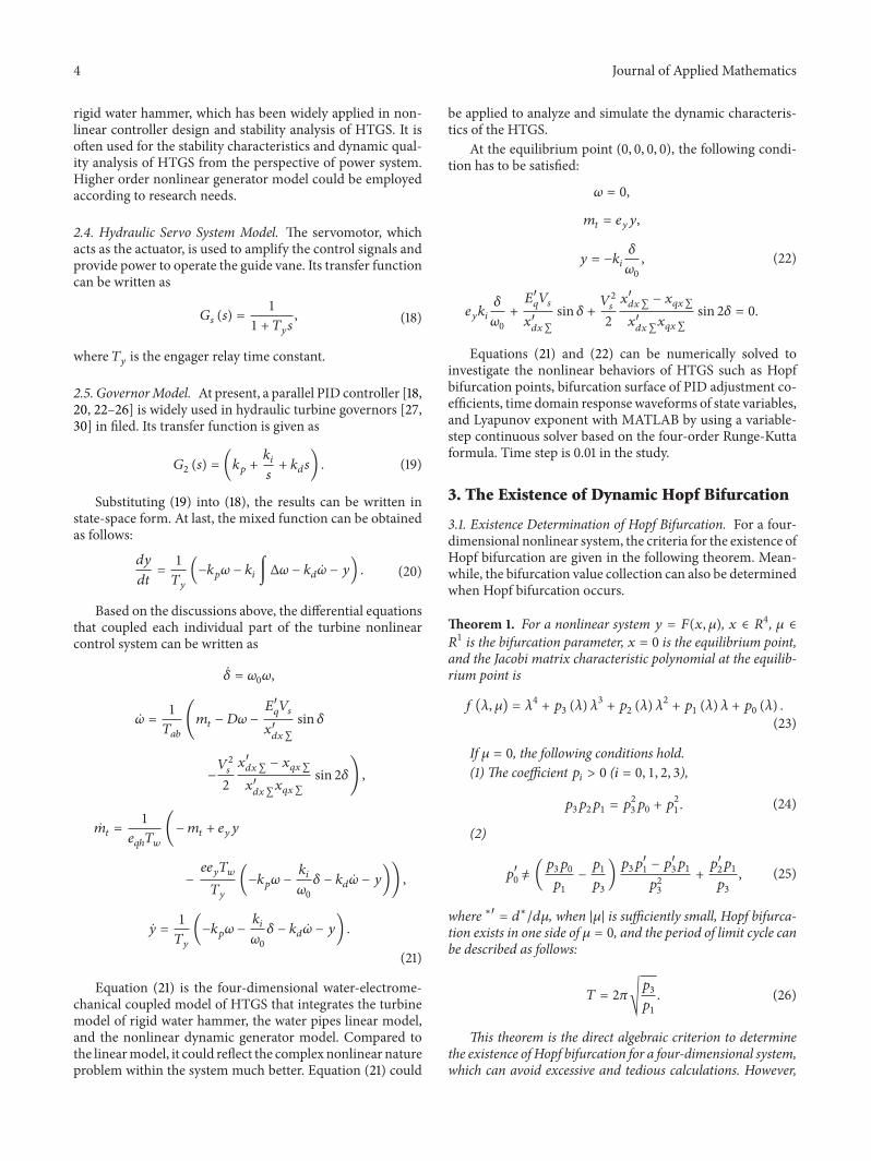
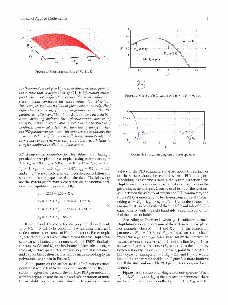
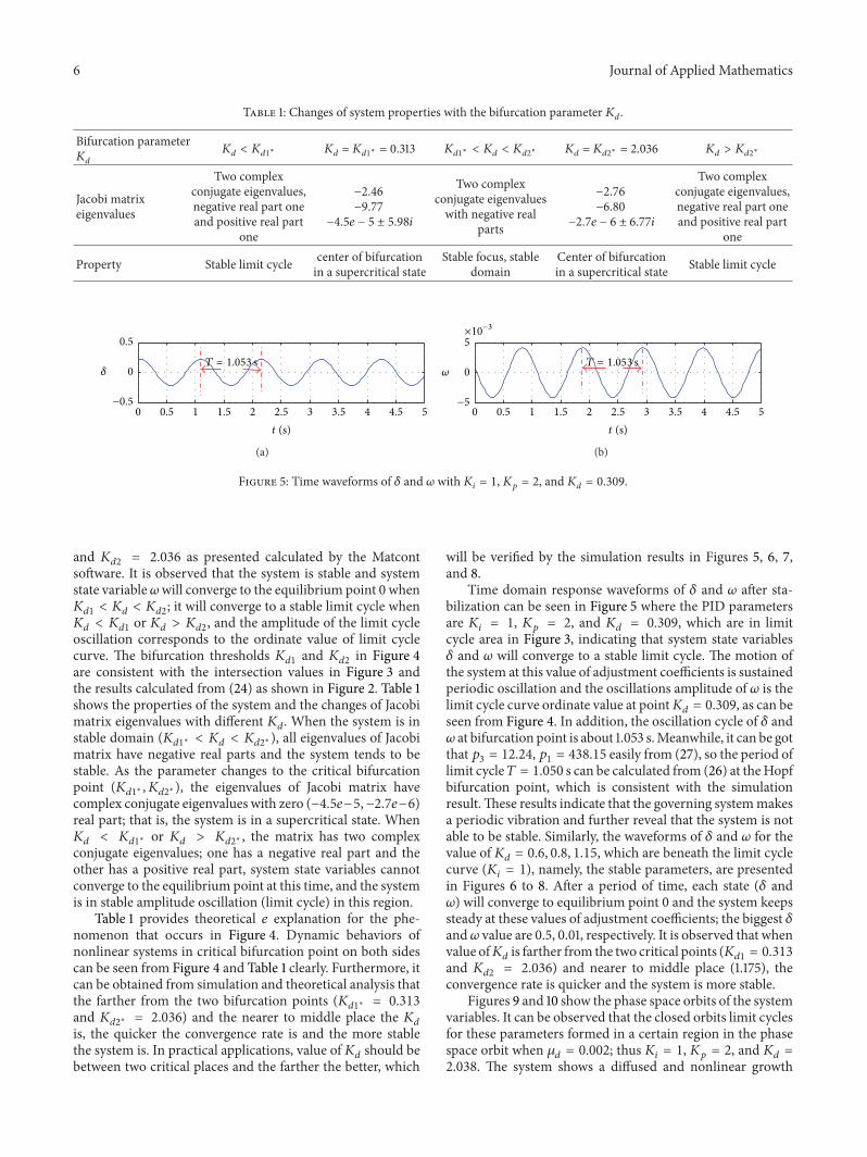
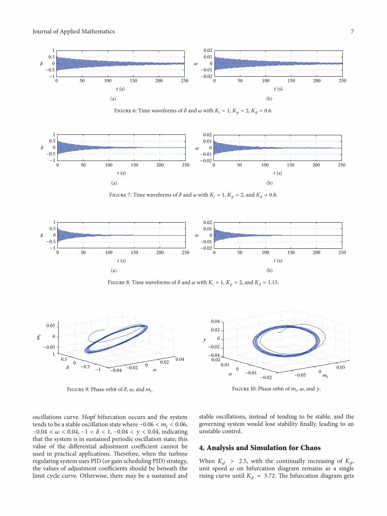
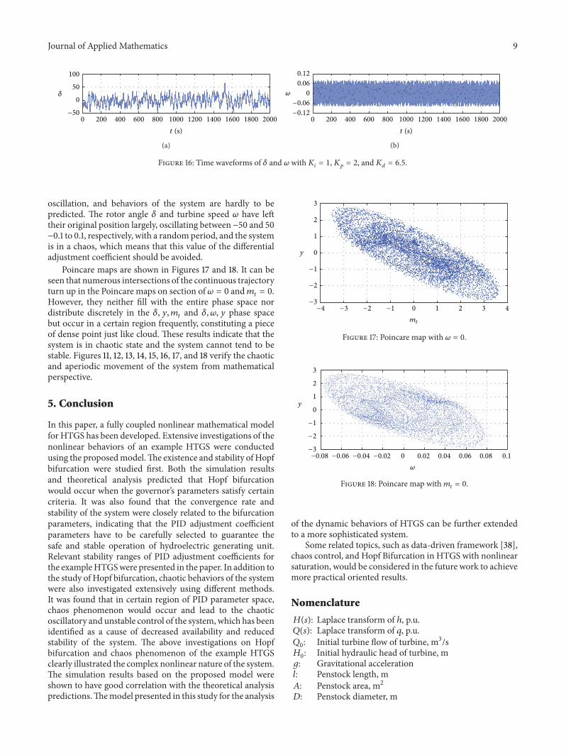
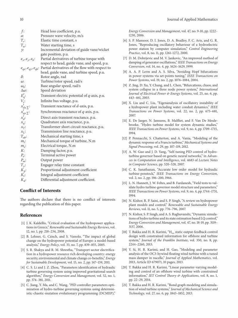
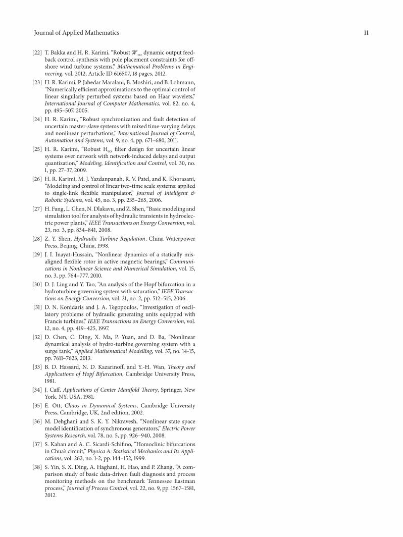


![Sparse Identification of Nonlinear Dynamical …arXiv:2005.13232v1 [stat.ML] 27 May 2020 Sparse Identification of Nonlinear Dynamical Systems via Reweighted ℓ1-regularized Least](https://img.pdfslide.us/doc/110x75/5fbe8824ad344c04ec197bab/sparse-identification-of-nonlinear-dynamical-arxiv200513232v1-statml-27-may.jpg)


![Studies on Integrability for Nonlinear Dynamical Systems ...tau.doshisha.ac.jp/d-thesis.pdf · Studies on Integrability for Nonlinear Dynamical Systems ... [89] by Zabusky and Kruskal](https://img.pdfslide.us/doc/110x75/5b7a33df7f8b9a460c8b60bd/studies-on-integrability-for-nonlinear-dynamical-systems-tau-studies-on.jpg)