Bayesian inference: basic operations

Probabilistic Models, Spring 2013 Petri Myllymäki, University of Helsinki II-1

22.01.13

Bayesian inference: basic operations


22.01.13

Probability of propositions● Notation P(x) : read “probability of “x-pression”

● Expressions are statements about the contents of random variables

● Random variables are very much like variables in computer programming languages.

– Boolean; statements, propositions

– Enumerated, discrete; small set of possible values

– Integers or natural numbers; idealized to infinity

– Floating point (continuous); real numbers to ease calculations


22.01.13

Elementary “probositions”● P(X=x)– probability that random variable X has value x

● we like to use words starting with capital letters to denote random variables

● For example:– P(It_will_snow_tomorrow = true)

– P(The_weekday_I'll_graduate = sunday)

– P(Number_of_planets_around_Gliese_581 = 7)

– P(The_average_height_of_adult Finns = 1702mm)


22.01.13

Semantics of P(X=x)=p● So what does it mean?– P(The_weekday_I'll_graduate = sunday)=0.20

– P(Number_of_planets_around_Gliese_581 = 7)=0.3

● Bayesian interpretation:– The proposition is either true or false, nothing in

between, but we may be unsure about the truth. Probabilities measure that uncertainty.

– The greater the p, the more we believe that X=x:● P(X=x) = 1 : Agent totally believes that X = x. ● P(X=x) = 0 : Agent does not believe that X=x at all.


22.01.13

● Elementary propositions can be combined using logical operators ˄, ˅ and ¬.− like P(X=x ˄ ¬ Y=y) etc.− Possible shorthand: P(X ϵ S) − P(X≤x) for continuous variables

● Operator ∧ is the most common one, and often replaced by just comma like : P(A=a, B=b).

● Naturally other logical operators can also be defined as derivatives.

Compound “probositions”


22.01.13

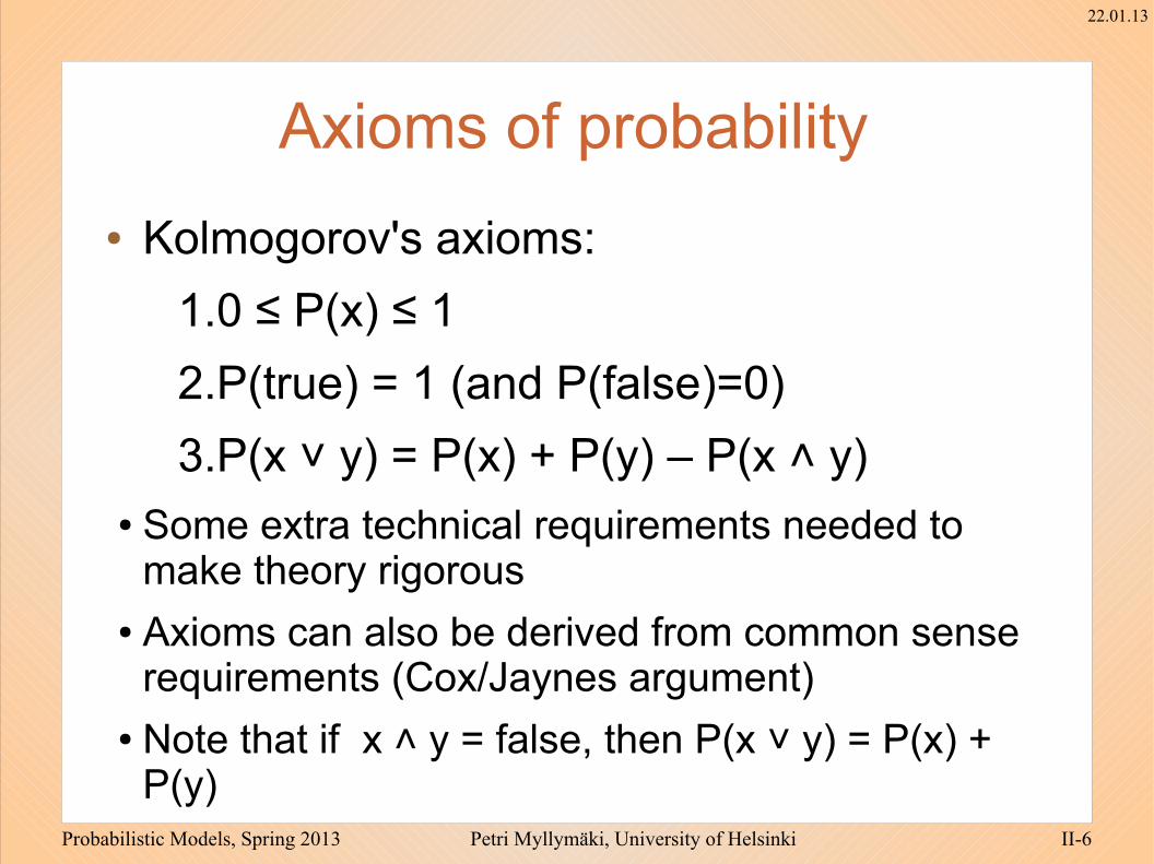
Axioms of probability

● Kolmogorov's axioms:

1.0 ≤ P(x) ≤ 1

2.P(true) = 1 (and P(false)=0)

3.P(x ˅ y) = P(x) + P(y) – P(x ˄ y)● Some extra technical requirements needed to

make theory rigorous● Axioms can also be derived from common sense

requirements (Cox/Jaynes argument)● Note that if x ˄ y = false, then P(x ˅ y) = P(x) +

P(y)


22.01.13

BA

Axiom 3 again– P(x or y) = P(x) + P(y) – P(x and y)

– It is there to avoid double counting:

– P(“day_is_sunday” or “day_is_in_July”) = 1/7 + 31/365 - 4/31.

A and B


22.01.13

Discrete probability distribution● Instead of stating that

• P(D=d1)=p

1,

• P(D=d2)=p

2,

• ... and

• P(D=dn)=p

n

● we often compactly say

– P(D)=(p1,p

2, ..., p

n).

● P(D) is called a probability distribution of D.

– NB! p1 + p

2 +

... + p

n = 1.

Mon Tue Wed Thu Fri

0

0,1

0,2

0,3

0,4

0,5

0,6

0,7

0,8

0,9

1

P(D)


22.01.13

Continuous probability distribution● In continuous case, the area under P(X=x)

must equal one. ● For example P(X=x) = exp(-x):


22.01.13

Main toolbox of the Bayesians● Definition of conditional probability● The chain rule● Marginalization (conditioning)● The Bayes rule

● NB. These are all direct derivates of the axioms of probability theory

● Also essential: definition of (conditional) independence


22.01.13

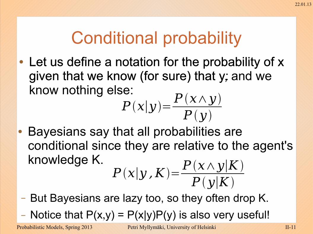
Conditional probability● Let us define a notation for the probability of x

given that we know (for sure) that y:

P x∣y =P x∧y P y

● Let us define a notation for the probability of x given that we know (for sure) that y, and we know nothing else:

● Bayesians say that all probabilities are conditional since they are relative to the agent's knowledge K.

●

– But Bayesians are lazy too, so they often drop K.

– Notice that P(x,y) = P(x|y)P(y) is also very useful!

P x∣y ,K =P x∧y∣K P y∣K


22.01.13

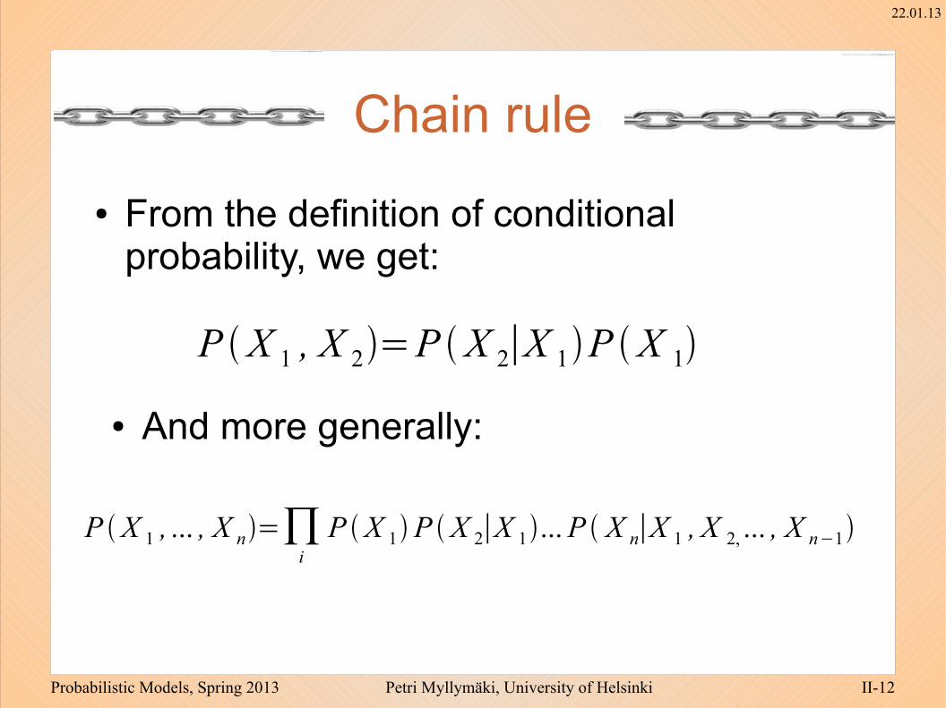
Chain rule

● From the definition of conditional probability, we get:

P X 1 , X 2=P X 2∣X 1P X 1

P X 1 , ... , X n=∏i

P X 1P X 2∣X 1...P X n∣X 1 , X 2, ... , X n−1

● And more generally:


22.01.13

Marginalization● Let us assume we have a joint probability

distribution for a set S of random variables.● Let us further assume S1 and S2 partitions the

set S.● Now ●

●

● where s1 and s are vectors of possible value

combination of S1 and S2 respectively.●

P S1=s1= ∑s∈dom S2

P S1=s1,S2=s

= ∑s∈domS2

P S1=s1∣S2=sP S2=s ,


22.01.13

● You may also think this as a P(Too_Cat_Cav=x), where x is a 3-dimensional vector of truth values.

● Generalizes naturally to any set of discrete variables, not only Booleans.

Joint probability distribution

Toothache Catch Cavity probabilitytrue true true 0,108true true false 0,016true false true 0,012true false false 0,064false true true 0,072false true false 0,144false false true 0,008false false false 0,576

1,000

● P(Toothache=x,Catch=y,Cavity=z) for all combinations of truth values (x,y,z):


22.01.13

Joys of joint probability distribution● By summing those numbers from the joint

probability table that match the corresponding condition, you can calculate the probability of any subset of events.

● E.g. P(Cavity=true or Toothache=true):Toothache Catch Cavity probabilitytrue true true 0,108true true false 0,016true false true 0,012true false false 0,064false true true 0,072false true false 0,144false false true 0,008false false false 0,576

0,280


22.01.13

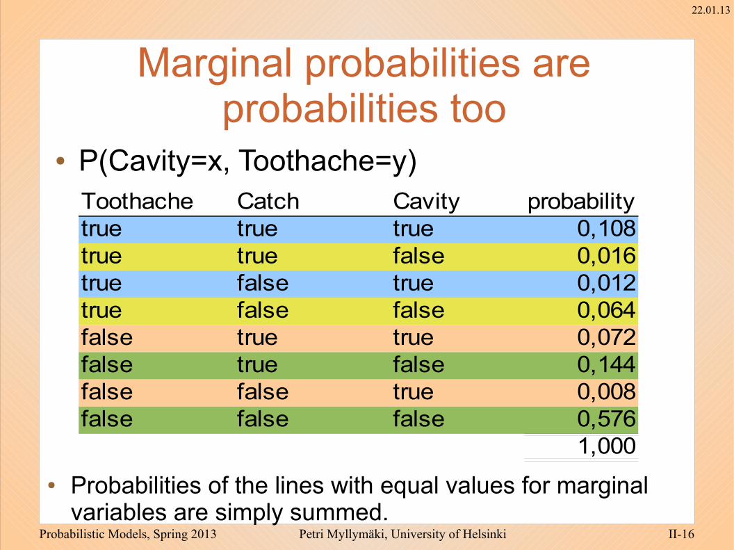
Marginal probabilities are probabilities too

● P(Cavity=x, Toothache=y)Toothache Catch Cavity probabilitytrue true true 0,108true true false 0,016true false true 0,012true false false 0,064false true true 0,072false true false 0,144false false true 0,008false false false 0,576

1,000

● Probabilities of the lines with equal values for marginal variables are simply summed.


22.01.13

Conditioning● Marginalization can be used to calculate

conditional probability:

PCavity=t∣Toothache=t =PCavity=t∧Toothache=t P Toothache=t

Toothache Catch Cavity probabilitytrue true true 0,108true true false 0,016true false true 0,012true false false 0,064false true true 0,072false true false 0,144false false true 0,008false false false 0,576

1,000

0.1080.0120.1080.0160.0120.064

=0.6


22.01.13

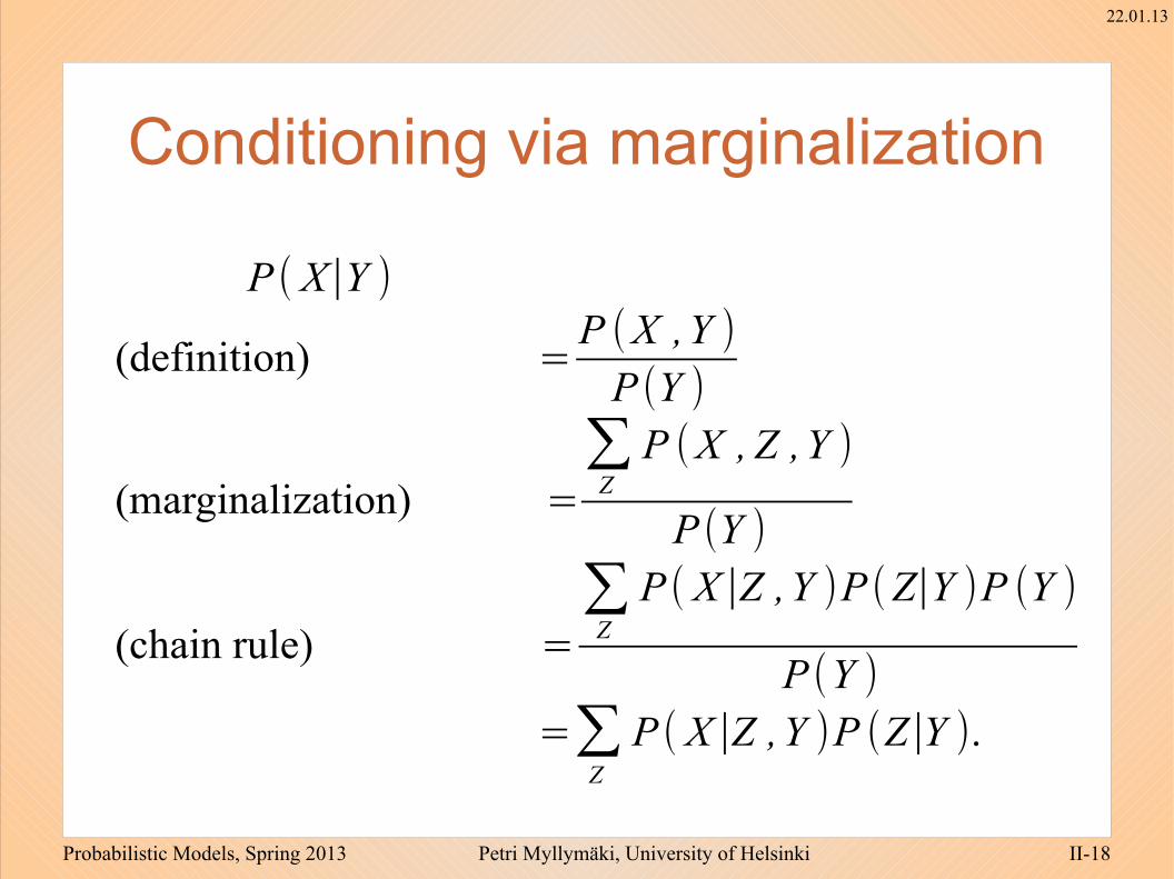
Conditioning via marginalization

P ( X∣Y )

(definition) =P (X ,Y )P (Y )

(marginalization) =∑Z

P (X , Z ,Y )

P (Y )

(chain rule) =∑Z

P( X∣Z ,Y )P (Z∣Y )P (Y )

P(Y )=∑

Z

P ( X∣Z ,Y )P (Z∣Y ).


22.01.13

The Bayes rule

● yields the famous Bayes formula

P (x∣y ,K )=P (x∧y∣K )P (y∣K )

P (x∧y∣K )=P (y∧x∣K )=P (y∣x ,K )P (x∣K )

P (x∣y ,K )=P (x∣K )P (y∣x ,K )

P (y∣K )

P (h∣e)=P (h)P (e∣h)

P (e)● or

● Combining


22.01.13

Bayes formula as an update rule● Prior belief P(h) is updated to posterior belief

P(h|e1). This, in turn, gets updated to P(h|e

1,e

2)

using the very same formula with P(h|e1) as a

prior. Finally, denoting P(·|e1) with P

1 we get

P (h∣e1,e2)=P (h,e1,e2)P (e1,e2)

=P (h,e1)P (e2∣h,e1)P (e1)P (e2∣e1)

=P (h∣e1)P (e2∣h ,e1)

P (e2∣e1)=P1(h)P1(e2∣h)

P1(e2)


22.01.13

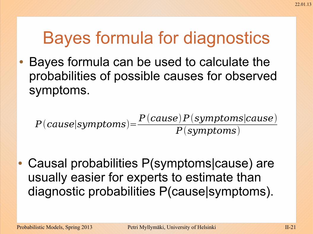
Bayes formula for diagnostics● Bayes formula can be used to calculate the

probabilities of possible causes for observed symptoms.

P (cause∣symptoms)=P (cause)P (symptoms∣cause)

P (symptoms)

● Causal probabilities P(symptoms|cause) are usually easier for experts to estimate than diagnostic probabilities P(cause|symptoms).


22.01.13

Bayes formula for model selection● Bayes formula can be used to calculate the

probabilities of hypotheses, given observations

P (H1∣D)=P (H1)P (D∣H1)

P (D)

P (H2∣D)=P (H2)P (D∣H2)

P (D)...


22.01.13

General recipe for Bayesian inference● X: something you don't know and need to

know● Y: the things you know● Z: the things you don't know and don't need

to know● Compute:

● That's it - we're done.

P (X∣Y )=∑Z

P ( X∣Z ,Y )P (Z∣Y )


22.01.13

Independence: definition● Let X, Y and Z be random variables.

● X ⊥ Y: X and Y are (marginally, i.e., unconditionally) independent if for all x,y holds: P(X=x,Y=y) = P(X=x)P(Y=y) .

● X ⊥ Y | Z: X and Y are conditionally independent given Z, if for all x,y,z with P(Z=z)>0 holds:

P(X=x,Y=y | Z=z) = P(X=x | Z=z)P(Y=y | Z=z).

● If two random variables are not (conditionally) independent, they are (conditionally) dependent


22.01.13

Importance of dependence/independence relations

● The naive structureless probabilistic approach: a look-up table for P(X1, X2,...,Xn) and direct application of probability calculus.

− Intractable computationally even for small n: For instance, with n=100 and binary variables, the table size is 2100. To calculate P(x1,...,x80 | x81,...,x100), we need to add up 280 numbers

− Difficult to understand and interpret, dependence structures are buried in a table of numbers

− Difficult to specify P in the first place

● Key dependence relations, such as direct interaction (cause-effect), are often

− what we are interested to discover

− qualitative building blocks of a modular model that are easy to understand and manipulate computationally


22.01.13

Bayesian inference: the Bernoulli model


22.01.13

Generative model

DataGenerates

● The world is described by a model that governs the probabilities of observing different kinds of data.

ϴ


22.01.13

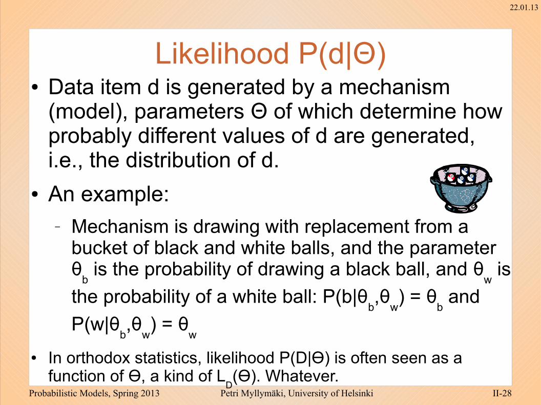
● Data item d is generated by a mechanism (model), parameters Θ of which determine how probably different values of d are generated, i.e., the distribution of d.

● An example:− Mechanism is drawing with replacement from a

bucket of black and white balls, and the parameter θ

b is the probability of drawing a black ball, and θ

w is

the probability of a white ball: P(b|θb,θ

w) = θ

b and

P(w|θb,θ

w) = θ

w

● In orthodox statistics, likelihood P(D|ϴ) is often seen as a function of ϴ, a kind of L

D(ϴ). Whatever.

Likelihood P(d|Θ)


22.01.13

i.i.d.● If the data generating mechanism depends on

ϴ only (and not on what has been generated before), the sequence of data data is called independent and identically distributed.

● Then ● And

− order of di does not matter.

−

P d1,d2,,dn∣=∏i=1

n

P di∣

P b,w ,b ,b ,w∣=P b,b ,w ,w ,w∣=P b∣P b∣P w∣P w∣P w∣


22.01.13

The Bernoulli model● A model for i.i.d. binary outcomes (heads,tails),

(1,0), (black, white), (true, false),....● One parameter: ϴ ϵ [0,1]. For example:

P(d=true | ϴ) = ϴ, P(d=false| ϴ) = 1-ϴ.− NB! The probabilities of d being true are defined by

the parameter ϴ. Parameters are not probabilities.− Black and white ball bucket as a Bernoulli model:

• ϴ is the proportion of black balls in a bucket P(b | ϴ) = ϴ.

• P(D|ϴ) = ϴNb (1-ϴ)Nw, where Nb and N

w are numbers of

black and white balls in the data D. • NB! P(D|ϴ) depends on data D through N

b and N

w only

(=sufficient statistics)


22.01.13

Steps in Bayesian inference● Specify a set of generative probabilistic

models● Assign a prior probability to each model● Collect data● Calculate the likelihood P(data|model) of each

model● Use Bayes’ rule to calculate the posterior

probabilities P(model | data)● Draw inferences (e.g., predict the next

observation)


22.01.13

Example● You are installing WLAN-cards for different

machines. You get the WLAN-cards from the same manufacturer, and some of them are faulty.

● We are asking the question: “Is the next WLAN-card we are installing going to work?”

● We are allowed to have background knowledge of these cards (they have been reliable/unreliable in the past, the manufacturing quality has gone up/down etc.)


22.01.13

Assessing models

● Let A = “The WLAN-card is not faulty”, and B=~A

● A proportion model can be understood as a bowl with labeled balls (A,B)

● each model M(ϴ) is characterized by the number of A balls, ϴ is the proportion (Obs! Assume here that ϴ is discrete, i.e., only consider ϴ ϵ {0,0.1,0.2,…,1})


22.01.13

Our 11 models

0123456789

10

0 .1 .2 .3 .4 .5 .6 .7 .8 .9 1

A

B

M(ϴ)


22.01.13

Priors and the models

0123456789

10

0 .1 .2 .3 .4 .5 .6 .7 .8 .9 1

A

B

M(ϴ)

0 0.02 0.03 0.05 0.1 0.15 0.2 0.25 0.15 0.05 0P(M(ϴ))


22.01.13

The prior distribution P(M(ϴ))

0

0,05

0,1

0,15

0,2

0,25

0 .1 .2 .3 .4 .5 .6 .7 .8 .9 1

M


22.01.13

Prediction by model averaging

● A Bayesian predicts by model averaging: the uncertainty about the model is taken into account by weighting the predictions of the different alternative models M

i

(=marginalization over the unknown)

P X =∑i

P X∣M i P M i


22.01.13

So: the predictive probability is...● What is P(A), the probability that the next

WLAN-card is not faulty?

● ”Mean or average” model: ϴ =0.598● 60/40 odds a priori

P A=P A∣M 0.0P M 0.0P A∣M 0.1P M 0.1...P A∣M 1.0P M 1.0=0.00.020.03...0.0=0.598

0

0,05

0,1

0,15

0,2

0,25

0 .1 .2 .3 .4 .5 .6 .7 .8 .9 1

M


22.01.13

Enter some data ...● Assume that I have installed three WLAN-

cards: first was non-faulty (A), the two latter ones faulty (B), i.e., D={ABB}

● what are the updated (posterior) probabilities for the models M(ϴ)?

● Enter Bayes, for example for M(0.6):0.2

P M 0.6∣D =P D∣M 0.6 P M 0.6

P D


22.01.13

Calculating model likelihoods

● i.i.d.: we assume that the observations are independent given any particular model M(ϴ)

● P(ABB | M(0.6)) = 0.6 * 0.4 * 0.4 = 0.096● This is repeated for each model M(ϴ)

To calculate the likelihood of a model, multiply theprobabilities of the individual observations given the model


22.01.13

Likelihood histogram P(ABB|M(ϴ))

0

0,05

0,1

0,15

0,2

0,25

0 .1 .2 .3 .4 .5 .6 .7 .8 .9 1

M


22.01.13

Posterior = likelihood x prior

0

0,05

0,1

0,15

0,2

0,25

0 .1 .2 .3 .4 .5 .6 .7 .8 .9 1

M X0

0,05

0,1

0,15

0,2

0,25

0 .1 .2 .3 .4 .5 .6 .7 .8 .9 1

M

=0

0,05

0,1

0,15

0,2

0,25

0 .1 .2 .3 .4 .5 .6 .7 .8 .9 1

M

P M ∣D∝P D∣M P M


22.01.13

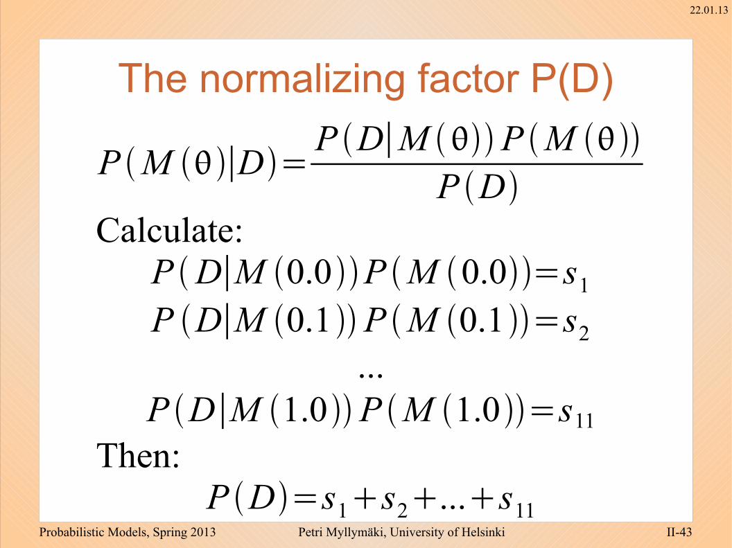
The normalizing factor P(D)

P M ∣D=P D∣M P M

P DCalculate:P D∣M 0.0P M 0.0=s1

P D∣M 0.1P M 0.1=s2

...P D∣M 1.0P M 1.0=s11

Then:P D=s1s2...s11


22.01.13

Posterior distribution P(M(ϴ)|D)

0

0,05

0,1

0,15

0,2

0,25

0 .1 .2 .3 .4 .5 .6 .7 .8 .9 1

M


22.01.13

Predictive probability with data D● With data D, the prediction is based on

averaging over the models M(ϴ) weighted now by the posterior (instead of the prior used earlier) probability of the models:

P X∣D=∑i

P X∣M i , DP M i∣D


22.01.13

How did the probabilitieschange?

● The predictive probability P(A | D) = P(A|ABB) that the next (fourth) WLAN-card is OK came down from the prior 60% to 52% (the change is not great because the data set is small)


22.01.13

Densities for proportions● a richer set of models allows more precise

proportion estimates, but comes with a cost: the amount of calculations necessary increase proportionally

● we can move to consider infinite number of models

– each model ϴ is now a point on the interval from [0,1]

– we get a “smoothed” bar chart called a density P(ϴ)– ∫P(ϴ)dϴ=1– only collections of models can have a probability > 0


22.01.13

Bayesian inference with densities?● Using densities means that we no longer add

probabilities, but calculate areas● To represent “infinite bar charts” we use

curves that approximate the heights of bars● But how to predict with densities? We cannot

go over all the individual models as we did in the discrete case

● What about the prior?


22.01.13

Maximum likelihood● Given a data D, different values of ϴ yield

different probabilities P(D|ϴ). The parameters that yield the largest probability of P(D|ϴ) are called maximum likelihood parameters for the data D.− P(b,b,w,w,w|Θ=0.7) = 0.720.33=0.1323− P(b,b,w,w,w|Θ=0.1) = 0.120.93=0.00729

− argmaxϴ P(b,b,w,w,w|ϴ) = argmax

ϴ ϴ2(1-ϴ)3=?


22.01.13

Likelihood P(b,b,w,w,w|Θ)

0 0.1 0.2 0.3 0.4 0.5 0.6 0.7 0.8 0.9 1.00

0,01

0,01

0,02

0,02

0,03

0,03

0,04

0,04

P(D|theta)

●NB! Not a distribution, but a function of ϴ.


22.01.13

ML-parameters for the Bernoulli model.(High school math refresher)

● So let us find ML-parameters for the Bernoulli model for the data with N

b black balls and N

w

white ones.P D∣=Nb 1−Nw ,so let us check when P ' D∣=0,∈]0,1[ .P 'D∣=Nb

Nb−1 1−NwNbNw1−Nw−1⋅−1

=Nb−11−Nw−1[Nb1−−Nw]=Nb−11−Nw−1[Nb−NbNw]=0

⇔Nb−NbNw=0 ⇔=Nb

NbNw


22.01.13

But ML-parameters are too gullible● Assume D=(w,w), i.e., two white balls.

− ML-parameter is Θ=0. − Now P(next ball is black | Θ=0)= 0. − Selecting ML parameters do not appear to be a

rational choice.

● Be Bayesian:− Parameters are exactly the things you do not know

for sure, so they have a (prior and posterior) distribution.

− Posterior distribution of the model is the goal of the Bayesian data-analysis.


22.01.13

Predicting with posterior distribution

● Not a two phase process like in ML-case− first find ML parameters Θ.− then use them to calculate P(d|Θ).

● Instead: P d∣D= ∫∈

P ,d∣D

= ∫∈

P d∣ , DP ∣D

= ∫∈

P d∣P ∣D

● Bayesian prediction uses predictions P(d|ϴ) from all the models ϴ, and weighs them by the posterior probability P(ϴ|D) of the models.


22.01.13

Posterior for Bernoulli parameter● So likelihood P(D|ϴ) we can calculate.● How about the prior P(ϴ)?

− We should give a real number for each ϴ.• One way out: as earlier, use a discrete set of

parameters instead of continuous ϴ. (Works, is flexible, but does not scale up well.)

• Another way: Study calculus. ● And how about P D=∫

0

1

P P D∣d


22.01.13

● The form of the likelihood gives us a hint for a comfortable prior − P(D|ϴ) = ϴNb (1-ϴ)Nw

− If we define the P(ϴ) = c ϴα-1 (1-ϴ)β-1,

• c taking care that ∫P(ϴ)dϴ = 1, then

− P(ϴ)P(D|ϴ) = c ϴNb+α-1 (1-ϴ)Nw+β-1

● Thus updating from prior to posterior is easy: just use the formula for the prior, and update exponents α-1 and β-1 (conjugate prior).

Prior for Bernoulli model


22.01.13

P(ϴ) of a form c ϴα-1(1-ϴ)β-1 is called Beta(α,β) distribution

● The expected value of Θ is α/(α+β).● The normalizing constant is

c= 1

∫0

1

−1 1−−1d

=

,

where is thegamma function,a continuous versionof the factorial:

n=n−1!


22.01.13

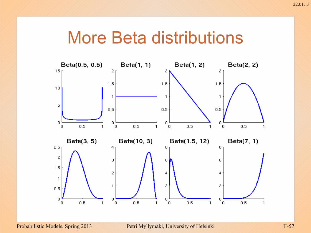
More Beta distributions


22.01.13

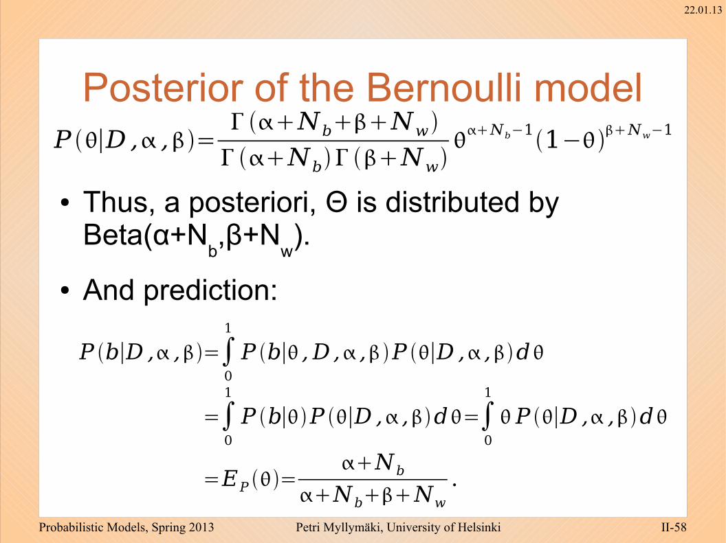
Posterior of the Bernoulli model

● Thus, a posteriori, Θ is distributed by Beta(α+N

b,β+N

w).

● And prediction:

P ∣D, ,= NbNw

Nb NwNb−11−Nw−1

P b∣D , ,=∫0

1

P b∣ , D , ,P ∣D , ,d

=∫0

1

P b∣P ∣D , ,d=∫0

1

P ∣D , ,d

=EP =Nb

NbNw

.


22.01.13

Bernoulli prediction

● So P(b|w,w,α=1,β=1) = (1+0) / (1+0+1+2) = 1/4.− Sounds more rational!− Notice how the hyperparameters α and β act

like extra counts.− That's why α + β is often called “equivalent

sample size”. The prior acts like seeing α black balls and β white balls before seeing data.

P b∣D, ,=Nb

NbNw

.


22.01.13

Laplace smoothing = Beta(1,1)● For Bayesian inference, we can use a single

model ϴ* which is the mean of the Beta(α,β) density:

• ϴ* = (α + N+)/(α + N+ + β + N-)

● E.g.: flip a coin 10 times, observe 7 heads (“success”). Assuming a uniform prior Beta(1,1), the posterior for the ϴ becomes Beta(8,4), and hence the predictive probability of heads is 8/12=2/3, or:− ϴ* = (7+1)/(10+2)

● Also known as Laplace’s rule of succession or Laplace smoothing


22.01.13

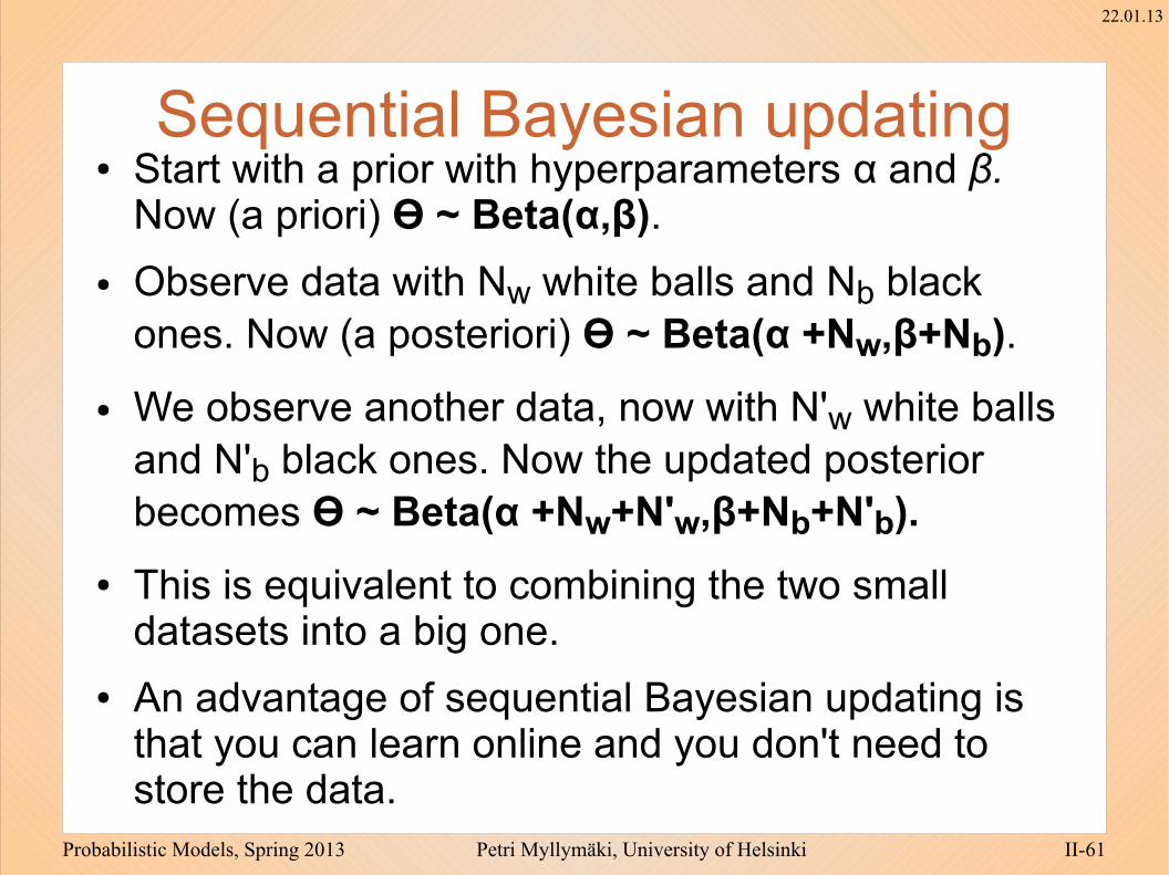
Sequential Bayesian updating● Start with a prior with hyperparameters α and β.

Now (a priori) ϴ ~ Beta(α,β).

● Observe data with Nw white balls and Nb black ones. Now (a posteriori) ϴ ~ Beta(α +Nw,β+Nb).

● We observe another data, now with N'w white balls and N'b black ones. Now the updated posterior becomes ϴ ~ Beta(α +Nw+N'w,β+Nb+N'b).

● This is equivalent to combining the two small datasets into a big one.

● An advantage of sequential Bayesian updating is that you can learn online and you don't need to store the data.


22.01.13

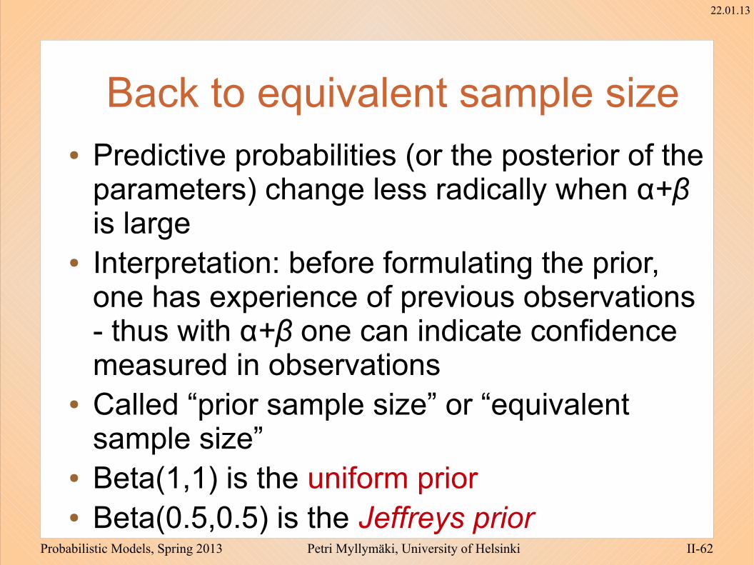
Back to equivalent sample size● Predictive probabilities (or the posterior of the

parameters) change less radically when α+β is large

● Interpretation: before formulating the prior, one has experience of previous observations - thus with α+β one can indicate confidence measured in observations

● Called “prior sample size” or “equivalent sample size”

● Beta(1,1) is the uniform prior● Beta(0.5,0.5) is the Jeffreys prior


22.01.13

Effect of the prior


22.01.13

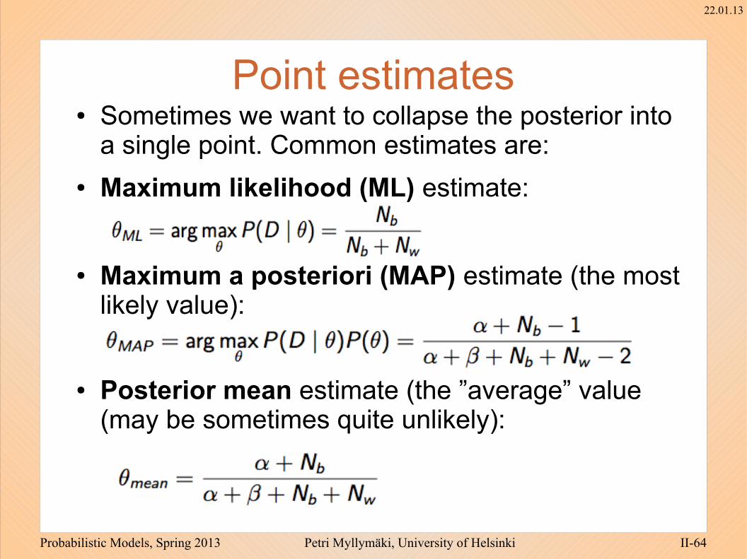
Point estimates● Sometimes we want to collapse the posterior into

a single point. Common estimates are:

● Maximum likelihood (ML) estimate:

● Maximum a posteriori (MAP) estimate (the most likely value):

● Posterior mean estimate (the ”average” value (may be sometimes quite unlikely):


22.01.13

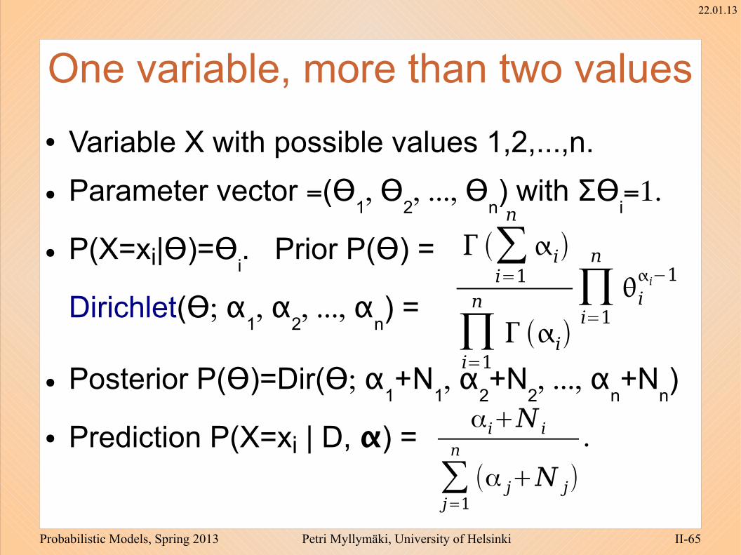
● Variable X with possible values 1,2,...,n.

● Parameter vector =(ϴ1, ϴ

2, ..., ϴ

n) with Σϴ

i=1.

● P(X=xi|ϴ)=ϴi. Prior P(ϴ) =

Dirichlet(ϴ; α1, α

2, ..., α

n) =

● Posterior P(ϴ)=Dir(ϴ; α1+N

1, α

2+N

2, ..., α

n+N

n)

● Prediction P(X=xi | D, α) =

One variable, more than two values

∑i=1

n

i

∏i=1

n

i∏i=1

n

ii−1

αi+N i

∑j=1

n

(α j+N j).

http://en.wikipedia.org/wiki/Dirichlet_distribution

Documents

Bayesian inference: basic operations