Bayesian Guided Pattern Search for Robust Local Optimization

Bayesian Guided Pattern Search forRobust Local Optimization

Matthew A. TADDY

Booth School of BusinessUniversity of Chicago

Chicago, IL 60637([email protected])

Herbert K. H. LEE

Department of Applied Mathematics and StatisticsUniversity of California Santa Cruz

Santa Cruz, CA 95064

Genetha A. GRAY

Sandia National LaboratoriesLivermore, CA 94551

Joshua D. GRIFFIN

SAS InstituteCary, NC 27513

Optimization for complex systems in engineering often involves the use of expensive computer simula-tion. By combining statistical emulation using treed Gaussian processes with pattern search optimization,we are able to perform robust local optimization more efficiently and effectively than when using eithermethod alone. Our approach is based on the augmentation of local search patterns with location sets gener-ated through improvement prediction over the input space. We further develop a computational frameworkfor asynchronous parallel implementation of the optimization algorithm. We demonstrate our methods ontwo standard test problems and our motivating example of calibrating a circuit device simulator.

KEY WORDS: Improvement statistics; Response surface methodology; Robust local optimization;Treed Gaussian process.

1. INTRODUCTION

Significant advances in computing capabilities and the risingcosts associated with physical experiments have contributed toincreases in both the use and complexity of numerical simu-lation. Often these models are treated as an objective functionto be optimized, such as in the design and control of complexengineering systems. The optimization is characterized by theinability to calculate derivatives and by the expense of obtain-ing a realization from the objective function. Due to the costof simulation, it is essential that the optimization converge rel-atively quickly. A search of the magnitude required to guaran-tee global convergence is not feasible. But at the same time,these large engineering problems are often multimodal, and itis possible to get stuck in low-quality solutions. We thus wishto take advantage of existing local optimization methods (i.e.,algorithms that locate a function optimum nearby to a specifiedstart location) for quick convergence, but use a statistical analy-sis of the entire function space to facilitate a global search andprovide more robust solutions.

We argue for the utility of using the predicted objective func-tion output over unobserved input locations, through statisti-cal emulation in the spirit of the analysis of computer exper-iments (e.g., Kennedy and O’Hagan 2001; Santner, Williams,and Notz 2003; Higdon et al. 2004), to act as a guide for under-lying local optimization. Thus our framework could be classi-fied as an oracle optimization approach (see Kolda, Lewis, andTorczon 2003 and references therein), where information fromalternative search schemes is used to periodically guide a rela-tively inexpensive local optimization. In particular, we proposea hybrid algorithm, referred to as TGP–APPS, which uses pre-diction based on nonstationary treed Gaussian process (TGP)modeling to influence an asynchronous parallel pattern search(APPS) through changes to the search pattern. Based on the pre-

dicted improvement statistics (see, e.g., Schonlau, Welch, andJones 1998) at a dense random set of input locations, candidatepoints are ranked using a novel recursive algorithm, and a pre-determined number of top-ranked points are added to the searchpattern. Both APPS- and the TGP-based generation of candi-date locations produce discrete sets of inputs that are queuedfor evaluation, and the merging of these two search patternsprovides a natural avenue for communication between compo-nents. This same property makes the methodology readily par-allelizable and efficient to implement. We argue that in manysituations, the approach will offer a robust and effective alter-native to algorithms based only on either a global statisticalsearch or a local pattern search. In addition, although we re-fer specifically to APPS and TGP throughout and have foundsuccess with these methods, our parallel scheme encompassesa general approach to augmenting local search patterns with sta-tistically generated location sets, and we emphasize that otherresearchers may find success using alternative methods for sta-tistical emulation or for parallel search.

The article is organized as follows. In Sections 2.1 and 2.2,we describe the methodological components underlying ourapproach—local optimization through APPS and statistical em-ulation of the objective function with TGP. We present the novelhybrid algorithm, combining APPS with TGP, in Section 3, anddetails for generating ranked global search patterns based onstatistical emulation in Section 3.1. We present an initial de-sign framework, including an informed sampling of the inputspace and sensitivity analysis, in Section 3.2. In Section 3.3 weoutline a framework for the asynchronous parallel implemen-

© 2009 American Statistical Association andthe American Society for Quality

TECHNOMETRICS, NOVEMBER 2009, VOL. 51, NO. 4DOI 10.1198/TECH.2009.08007

389

Dow

nloa

ded

by [1

07.1

0.14

8.4]

at 1

2:07

10

Dec

embe

r 201

2

mailto:[email protected]

http://www.amstat.org

http://www.asq.org

http://pubs.amstat.org/loi/tech

http://dx.doi.org/10.1198/TECH.2009.08007

390 MATTHEW A. TADDY ET AL.

tation of our hybrid optimization algorithm and present resultsfor two standard test problems (introduced in the next section).In Section 4 we illustrate our methods on our motivating exam-ple involving calibration of a circuit device simulator. Finally,in Section 5 we investigate convergence and begin to considerhow statistical information can be used to assess the quality ofconverged solutions.

1.1 Examples

To illustrate the methodology throughout this paper, weconsider two common global optimization test functions, theRosenbrock and Shubert problems. Both involve minimizationof a continuous response, f (x), over a bounded region for inputsx = [x1, x2] ∈ R2. Specifically, the two-dimensional Rosen-brock function is defined as

f (x) = 100(x21 − x2)

2 + (x1 − 1)2, (1)

where herein −1 ≤ xi ≤ 5 for i = 1,2 and the Shubert functionis defined as

f (x) =( 5∑

j=1

j cos((j + 1)x1 + j)

)

×( 5∑

j=1

j cos((j + 1)x2 + j)

)

, (2)

where −10 ≤ xi ≤ 10 for i = 1,2. The global solution of theRosenbrock problem is x! = (1,1) for f (x!) = 0, and the Shu-bert problem has 18 global minima x! with f (x!) = −186.7309(problem descriptions from Hedar and Fukushima 2006).

The response surfaces are shown in the background of Fig-ure 1. These problems emphasize some particular difficul-ties associated with optimization algorithms. The plotted log-response surface for the Rosenbrock function shows a steepvalley with a gradually sloping floor. The solution lies at theend of this long valley, and the combination of steep gradientsup the valley walls and gradual gradients along the valley floorwill typically cause problems for local search methods, such asgradient descent and pattern search. As shown on the right sideof Figure 1, the Shubert problem is characterized by rapid oscil-

Figure 1. Rosenbrock (left) and Shubert (right) test problems.The response surface images (log response for Rosenbrock) are risingfrom white to black, and trace paths for the best point during optimiza-tion are shown as a dotted line for APPS, a dashed line for APPS–TGP,and a solid line for APPS–TGP following initialization through Latinhypercube sampling.

lations of the response surface. There are multiple minima, eachof which is located adjacent to dual local maxima, thus present-ing a challenging problem for global optimization methods thatwill tend to over explore the input space or miss a minimumhidden among the maxima.

Each of these problems illustrates different aspects of our al-gorithm. The Rosenbrock problem is specifically designed tocause local pattern search methods to break down. The mo-tivation for considering this problem is to show the poten-tial for TGP–APPS to overcome difficulties in the underlyingpattern search and also to significantly decrease computationtime in certain situations. Conversely, the Shubert problem issolved relatively easily through standard pattern search meth-ods, whereas the presence of multiple global minima wouldcause many algorithms based solely on statistical predictionto overexplore the input space and lead to higher than neces-sary computation costs. Indeed, the APPS optimization doesconverge, on average, in about half the iterations used byTGP–APPS; however, this is a small increase in computationcompared with what would be required by many fully globaloptimization routines (e.g., genetic algorithms, simulated an-nealing). Moreover, the results for APPS–TGP may be consid-ered more robust; the global scope of the TGP search protectsagainst premature convergence to a local optimum. The benefitof this additional robustness is clearly illustrated in the real-world application of Section 4.

2. ELEMENTS OF THE METHODOLOGY

The optimization algorithm is based on point locations sug-gested either by asynchronous parallel pattern search or througha statistical analysis of the objective function based on TGPs.We outline these two methodological elements in Sections 2.1and 2.2. As is the case throughout, all algorithms and exampleshave minimization as the unstated goal.

2.1 Asynchronous Parallel Pattern Search

Pattern search is included in a class of derivative-free opti-mization methods developed primarily to address problems inwhich the derivative of the objective function is unavailable andapproximations are unreliable (Wright 1996). The optimizationuses a predetermined pattern of points to sample a given func-tion domain and is considered a direct search algorithm (Kolda,Lewis, and Torczon 2003), with no attempt made to explicitlyevaluate or estimate local derivatives. This type of optimizeris considered more robust than derivative-based approaches fordifficult optimization problems with nonsmooth, discontinuous,or undefined points.

The APPS algorithm is much more complicated than sim-ple pattern search, requiring careful bookkeeping. Thus here weprovide only a brief outline of the basic steps, referring the moreinterested reader to work of Kolda (2005) and Kolda (2006). Ateach iteration k of APPS, three basic steps are executed:

1. Generate a set of trial points, Qk, around the current bestpoint xbest

k (defined later).2. Send trial points Qk to the compute cluster, and obtain a

set of function evaluations Rk.3. Update the best point, xbest

k+1.

TECHNOMETRICS, NOVEMBER 2009, VOL. 51, NO. 4

Dow

nloa

ded

by [1

07.1

0.14

8.4]

at 1

2:07

10

Dec

embe

r 201

2

BAYESIAN GUIDED PATTERN SEARCH FOR ROBUST LOCAL OPTIMIZATION 391

Convergence to locally optimal points is ensured using a suf-ficient decrease criterion for accepting new best points. Anincoming trial point, x′, is considered a new best point iff (x′)− f (xbest

k ) < δ, for user-defined δ > 0. In the unconstrainedcase, using standard assumptions, it can be shown that

lim infk→∞

‖∇f (xbestk )‖ → 0.

Similar optimality results can be shown for linearly constrainedoptimization in terms of projections onto local tangent cones(Kolda, Lewis, and Torczon 2006).

Trial points are generated using a positive spanning set ofsearch directions {d1, . . . ,dL} and have the form Qk = {xbest

k +#kldl|1 ≤ l ≤ L}, for positive step sizes #kl. The step sizes andsearch directions are chosen as described by Gray and Kolda(2006). After a successful iteration (one in which a new bestpoint has been found), the step size is either left unchanged orincreased. But, if the iteration was unsuccessful, then the stepsize is reduced. A defining difference between simple patternsearch and APPS is that for APPS, directions are processedindependently, and each direction may have its own step size.Because of the asynchronous environment, the members of Qkgenerally will not all be returned in Rk+1, but instead will bespread throughout the next several R’s. Thus APPS needs to beable to deal with the fact that the function evaluations may bereturned in a different order than requested, and that the gen-eration of the next iteration of trial points Qk+1 may need tobe created before all of the results of the previous iteration areavailable.

This algorithm has been implemented in an open sourcesoftware package called APPSPACK and has been success-fully applied to problems in microfluidics, biology, ground-water, thermal design, and forging (see Gray and Kolda 2006and references therein). The latest software is publicly avail-able at http:// software.sandia.gov/appspack/ . There are manyplausible competitors for APPS as a derivative-free optimiza-tion method (see, e.g., Fowler et al. 2008 for a thorough com-parison of a dozen such algorithms); keep in mind, however,that it is the parallelization of the APPS search that makes itparticularly amenable to a hybrid search scheme, and there arerelatively few available parallel methods. Our software devel-opment is exploring the use of alternative parallel search com-ponents, but none of these are as easily available or as widelydistributed as APPS.

2.2 Treed Gaussian Process Emulation

A Bayesian approach was brought to the emulation of com-puter code by Currin et al. (1991), who focused on the com-monly used GP model. Santner, Williams, and Notz (2003) fol-lowed a mainly Bayesian methodology and provided a detailedoutline of its implementation through examples. Standard prac-tice in the computer experiments literature is to model the out-put of the simulations as a realization of a stationary GP (Sackset al. 1989; O’Hagan, Kennedy, and Oakley 1998; Fang, Li, andSudjianto 2006). In this setting, the unknown function is mod-eled as a stochastic process: the response is a random variable,f (x), dependent on input vector x. In model specification, theset of stochastic process priors indexed by the process parame-ters and their prior distributions represents our prior uncertainty

regarding possible output surfaces. It is possible to model bothdeterministic and nondeterministic functions with these meth-ods. The basic GP model is f (x) = µ(x) + w(x), where µ(x) isa simple mean function, such as a constant or a low-order poly-nomial, and w(x) is a mean-0 random process with covariancefunction c(xi,xj). A typical approach would be to use a linearmean trend, µ(x) = xβ , and an anisotropic Gaussian correla-tion function,

c(xi,xj) = exp

[

−(

d∑

k=1

(xik − xjk)2

θk

)]

, (3)

where d is the dimension of the input space and θk is the rangeparameter for each dimension.

TGP models represent a natural extension of this method-ology and provide a more flexible nonstationary regressionscheme (Gramacy and Lee 2008). There is software available inthe form of a tgp library for the statistical package R (see http://www.cran.r-project.org/src/contrib/Descriptions/ tgp.html),which includes all of the statistical methods described in thisarticle. TGP models work by partitioning the input space intodisjoint regions in which an independent GP prior is assumed.Partitioning allows for the modeling of nonstationary behav-ior and can ameliorate some of the computational demand ofnonstationary modeling by fitting separate GPs to smaller datasets (the individual partitions). The partitioning is achieved in afashion derived from the Bayesian classification and regres-sion tree work of Chipman, George, and McCulloch (1998,2002). Our implementation uses reversible-jump Markov chainMonte Carlo (MCMC) (Green 1995) with tree proposal opera-tions (prune, grow, swap, change, and rotate) to simultaneouslyfit the tree and the parameters of the individual GP models.In this way, all parts of the model can be learned automaticallyfrom the data, and Bayesian model averaging through reversiblejump allows for explicit estimation of predictive uncertainty.The prior on the tree space is a process prior specifying thateach leaf node splits with probability a(1 + q)−b, where q isthe depth of the node and a and b are parameters chosen to givean appropriate size and spread to the distribution of trees. Weuse hierarchical priors for the GP parameters within each of thefinal leaf nodes ν. For each region ν, the hierarchical GP modelis

Zν |βν,σ2ν ,Kν ∼ Nnν (Fνβν,σ

2ν Kν),

β0 ∼ Nd+1(µ,B),

βν |σ 2ν , τ 2

ν ,W,β0 ∼ Nd+1(β0,σ2ν τ 2

ν W),

τ 2ν ∼ IG(ατ /2,qτ/2),

σ 2ν ∼ IG(ασ /2,qσ /2),

W−1 ∼ W((ρV)−1,ρ),

with Fν = (1,Xν), and W is a (d + 1)× (d + 1) matrix. The N,IG, and W are the (multivariate) normal, inverse-gamma, andWishart distributions. Hyperparameters µ, B, V, ρ, ασ , qσ , ατ ,and qτ are treated as known, and the default values from thetgp package are used. The coefficients βν are modeled hierar-chically with a common unknown mean β0 and region-specificvariance σ 2

ν τ 2ν . There is no explicit mechanism in this model

to ensure that the process is continuous across the partitions;


Dow

nloa

ded

by [1

07.1

0.14

8.4]

at 1

2:07

10

Dec

embe

r 201

2

http://software.sandia.gov/appspack/

http://www.cran.r-project.org/src/contrib/Descriptions/tgp.html

http://www.cran.r-project.org/src/contrib/Descriptions/tgp.html


however, the model can capture smoothness through model av-eraging, as predictions are integrated over the tree space, sowhen the true function is smooth, the predictions will be aswell. When the data actually indicate a nonsmooth process, theTGP retains the flexibility necessary to model discontinuities.One further advantage of TGP over a standard GP is in com-putational efficiency—fitting a Bayesian GP requires repeatedinversion of an n×n matrix (where n is the sample size), requir-ing O(n3) computation time. By partitioning the space, eachregion contains a smaller subsample, thereby significantly de-creasing the computational effort. Further details of implemen-tation and properties for TGP have been given by Gramacy andLee (2008). We note that other emulators, such as neural net-works, could be considered; however, we prefer the GP/TGPfamily because of the ability to ensure a degree of smoothnessin the fitted function, the ability to model nonstationarity, andthe robustness in the fitting of the model.

The TGP model involves a complex prior specification topromote mixing over alternative tree structures. However, theprior parameterization provided as a default for the tgp soft-ware is designed to work out-of-the-box in a wide variety ofapplications. In all of the examples in this article, including thecircuit application of Section 4, after both input and responsehave been scaled to have mean 0 and variance 1, process andtree parameters were assigned the default priors from the tgpsoftware (Gramacy 2007). Here each partition has a GP of theform (3), but with an additional nugget parameter in the cor-relation structure. Each range parameter θk has prior π(θk) =gamma(1,20)/2 + gamma(10,10)/2, where gamma(a,b) hasexpectation a/b. The covariance for (xi,xj) within the sametree partition is then σ 2(c(xi,xj)+ γ ), with σ 2 the GP varianceand γ the nugget parameter. The nugget term requires the onlynondefault parameterization, due to the fact that we are model-ing deterministic objective functions that do not involve randomnoise. Although we do not completely remove accommodationof random error from the model, γ is forced to be small throughthe prior specification π(γ ) = gamma(1,100) (as opposed tothe default gamma(1,1) for noisy response surfaces). The pres-ence of a small nugget allows for smoothing of the predicted re-sponse surface to avoid the potential instability that is inherentin point-by-point interpolation. This smoothing is made possi-ble through the hybridization; because the local optimizationrelies on pattern search rather than the TGP predicted response,it is more important that the statistical modeling be globally ap-propriate than that it be a perfect interpolator. We note that thenugget also allows for the possibility of numerical instability incomplex simulators, and it improves numerical stability of thecovariance matrix inversions required during MCMC.

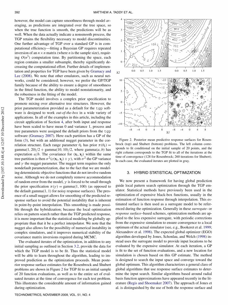
The evaluated iterates of the optimization, in addition to anyinitial sampling as outlined in Section 3.2, provide the data forwhich the TGP model is to be fit. Thus the statistical modelwill be able to learn throughout the algorithm, leading to im-proved prediction as the optimization proceeds. Mean poste-rior response surface estimates for the Rosenbrock and Shubertproblems are shown in Figure 2 for TGP fit to an initial sampleof 20 function evaluations, as well as to the entire set of eval-uated iterates at the time of convergence for each test problem.This illustrates the considerable amount of information gainedduring optimization.

Figure 2. Posterior mean predictive response surfaces for Rosen-brock (top) and Shubert (bottom) problems. The left column corre-sponds to fit conditional on the initial sample of 20 points, and theright column corresponds to the TGP fit to all of the iterations at thetime of convergence (128 for Rosenbrock; 260 iterations for Shubert).In each case, the evaluated iterates are plotted in gray.

3. HYBRID STATISTICAL OPTIMIZATION

We now present a framework for having global predictionguide local pattern search optimization through the TGP em-ulator. Statistical methods have previously been used in theoptimization of expensive black-box functions, usually in theestimation of function response through interpolation. This es-timated surface is then used as a surrogate model to be refer-enced during the optimization. Generally in these surrogate- orresponse surface–based schemes, optimization methods are ap-plied to the less expensive surrogate, with periodic correctionsfrom the expensive simulation to ensure convergence to a localoptimum of the actual simulator (see, e.g., Bookeret et al. 1999;Alexandrov et al. 1998). The expected global optimizer (EGO)algorithm developed by Jones, Schonlau, and Welch (1998) in-stead uses the surrogate model to provide input locations to beevaluated by the expensive simulator. At each iteration, a GPis fit to the set of function evaluations, and a new location forsimulation is chosen based on this GP estimate. The methodis designed to search the input space and converge toward theglobal optimum. This algorithm characterizes a general class ofglobal algorithms that use response surface estimates to deter-mine the input search. Similar algorithms based around radialbasis function approximations have appeared recently in the lit-erature (Regis and Shoemaker 2007). The approach of Jones etal. is distinguished by the use of both the response surface and


Dow

nloa

ded

by [1

07.1

0.14

8.4]

at 1

2:07

10

Dec

embe

r 201

2


the estimation error across this surface in choosing new inputlocations. This is achieved through improvement statistics, andthese feature prominently in our methods.

Although the optimization approach presented here has sim-ilarities to these response surface global algorithms, the under-lying motivation and framework are completely distinct. More-over, existing response surface methodologies rely either on asingle point estimate of the objective surface or, in the case ofthe EGO and related algorithms, point estimates of the parame-ters governing the probability distribution around the responsesurface. Conversely, our analysis is fully Bayesian and is fit-ted using MCMC, providing a sample posterior predictive dis-tribution for the response at any desired location in the inputspace. Full posterior sampling is essential to our algorithm forthe ranking of a discrete input set, and because TGP modelingis not the sole source for new search information, the compu-tational expense of MCMC prediction is acceptable. We arguethat the cost associated with restarts for a local optimizationalgorithm (a standard approach for checking robustness) willquickly surpass that of our more coherent approach in all butthe fastest and smallest optimization problems. In combiningAPPS with TGP, our goal is to provide global scope to an in-herently local search algorithm. The solutions obtained throughthe hybrid algorithm will be more robust than those obtainedthrough any isolated pattern search. But in addition, we haveobserved that the hybrid algorithm can lead to more efficientoptimization of difficult problems.

In this section we outline the main pieces of our optimiza-tion framework. In Section 3.1 we describe an algorithm to sug-gest additional search locations based on a statistical analysis ofthe objective function, in Section 3.2 we provide a frameworkfor initial sampling of the input space and sensitivity analysis,and in Section 3.3 we outline a general framework for efficientparallel implementation of such hybrid algorithms. Finally, wepresent the optimization results for our example problems inSection 3.4.

3.1 Statistically Generated Search Patterns

We focus on the posterior distribution of improvement statis-tics, obtained through MCMC sampling conditional on a TGPmodel fit to evaluated iterates, in building a location set to aug-ment the local search pattern. Improvement is defined here, fora single location, as I(x) = max{fmin − f (x),0}, where fmin isthe minimum evaluated response in the search (fmin may be lessthan the response at the present best point, as defined in Sec-tion 2.1 for the purpose of the local pattern search, due to thesufficient decrease condition). In particular, we use the poste-rior expectation of improvement statistics as a criterion for se-lecting input locations to be sent for evaluation. Note that theimprovement is always nonnegative, because points that do notturn out to be new minimum points still provide valuable infor-mation about the output surface. Thus in the expectation, can-didate locations will be rewarded for high response uncertainty(indicating a poorly explored region of the input space, suchthat the response could easily be lower than fmin) as well as forlow mean predicted response.

Schonlau, Welch, and Jones (1998) discussed improvementstatistics and proposed some variations on the standard im-provement that are useful in generating location sets. The ex-ponentiated Ig(x) = (max{(fmin − f (x)),0})g, where g is anonnegative integer, is a more general improvement statistic.Increasing g increases the global scope of the criteria by re-warding in the expectation extra variability at x. For example,g = 0 leads to E[I0(x)] = Pr(I(x) > 0) (assuming the conven-tion 00 = 0), g = 1 yields the standard statistic, and g = 2 ex-plicitly rewards the improvement variance because E[I2(x)] =var[I(x)] + E[I(x)]2. We have experienced some success witha g that varies throughout the optimization, decreasing as theprocess converges. In all of our examples, the algorithm be-gins with g = 2, and this changes to g = 1 once the maximumAPPS step size (max{#k1, . . . ,#kL} from Section 2.1) dropsbelow 0.05. But we have found the algorithm to be robust to thischoice, and a fixed g has not been found to hurt performance.Figure 3 illustrates expected improvement surfaces E[Ig(x)]with g = 1 and g = 2, for both the Shubert and Rosenbrockproblems, conditional on a TGP fit to the first 75 iterates of anoptimization run. The surfaces show only a subtle difference instructure across the different g parameterization; however, thiscan lead to substantially different search patterns based on theranking algorithm, which we describe next.

The TGP generated search pattern comprises m locations thatmaximize (over a discrete candidate set) the expected multilo-

Figure 3. Expected improvement surfaces E[Ig(x)] and ranks ofthe top 10 candidate locations, for the Rosenbrock (top) and Shubert(bottom) problems, conditional on TGP fit to 75 function evaluations.The plots on the left correspond to g = 1; those on the right, to g = 2.


Dow

nloa

ded

by [1

07.1

0.14

8.4]

at 1

2:07

10

Dec

embe

r 201

2


cation improvement, E[Ig(x1, . . . ,xm)], where

Ig(x1, . . . ,xm)

=(max

{(fmin − f (x1)), . . . , (fmin − f (xm)),0

})g (4)

(Schonlau, Welch, and Jones 1998). In most situations, findingthe maximum expectation of (4) will be difficult and expensive.In particular, it is impossible to do so for the full posterior dis-tribution of Ig(x1, . . . ,xm), and would require conditioning on asingle fit for the parameters of TGP. Our proposed solution is todiscretize the d-dimensional input space onto a dense candidateset X̃ of M locations. Although optimization over this set willnot necessarily lead to the optimal solution in the underlyingcontinuous input space, the use of APPS for local search meansthat such exact optimization is not required.

The discretization of decision space allows for a fast iterativesolution to the optimization of E[Ig(x1, . . . ,xm)]. This beginswith evaluation of the simple improvement Ig(x̃i) over x̃i ∈ X̃at each of T MCMC iterations (each corresponding to a sin-gle posterior realization of TGP parameters and predicted re-sponse) to obtain the posterior sample

I =

Ig(x̃1)1 · · · Ig(x̃M)1...

Ig(x̃1)T · · · Ig(x̃M)T

. (5)

We then proceed iteratively to build an ordered search patternof m locations: Designate x1 = argmaxx̃∈X̃ E[Ig(x̃)], and forj = 2, . . . ,m, given that x1, . . . ,xj−1 are already included in thesearch pattern, the next member is

xj = argmaxx̃∈X̃

E[max{Ig(x1, . . . ,xj−1), Ig(x̃)}

]

= argmaxx̃∈X̃

E[(

max{(fmin − f (x1)), . . . , (fmin − f (xj−1)),

(fmin − f (x̃)),0})g]

= argmaxx̃∈X̃

E[Ig(x1, . . . ,xj−1, x̃)].

Thus, after each jth additional point is added to the set, we havethe maximum expected j location improvement conditional onthe first j − 1 locations. This is not necessarily the uncondi-tionally maximal expected j location improvement; instead, thepoint xj is the location that will cause the greatest increase inexpected improvement over the given j − 1 location expectedimprovement.

Note that the foregoing expectations are all taken with re-spect to the posterior sample I , which acts as a discrete ap-proximation to the true posterior distribution for improvementat locations within the candidate set. Thus iterative selection ofthe point set is possible without any refitting of the TGP model.It follows that x1 = x̃i1 , the first location to be included in thesearch pattern, is such that the average of the i1th column of Iis greater than every other column average. Conditional on theinclusion of xi1 in the search pattern, a posterior sample of thetwo-location improvement statistics is calculated as

I2 =

Ig(x̃i1 , x̃1)1 · · · Ig(x̃i1, x̃M)1...

Ig(x̃i1 , x̃1)T · · · Ig(x̃i1, x̃M)T

, (6)

where the element in the tth row and jth column of this ma-trix is calculated as max{Ig(x̃i1)t, Ig(x̃j)t}. The second loca-tion in the search pattern, x2 = x̃i2 , is then chosen such thatthe i2th column of I2 is the column with the greatest mean.Similarly, Il, for l = 3, . . . ,m, has element (t, j) equal tomax{Ig(x̃i1, . . . , x̃il−1)t, Ig(x̃j)t} = Ig(x̃i1, . . . , x̃il−1, x̃j)t, and thelth location included in the search pattern corresponds to thecolumn of this matrix with maximum average. Because themultilocation improvement is always at least as high as the im-provement at any subset of those locations, the same points willnot be chosen twice for inclusion.

An appealing byproduct of this technique is that the searchpattern has been implicitly ordered, producing a ranked set oflocations that will be placed in the queue for evaluation. The 10top-ranked points corresponding to this algorithm, based on aTGP fit to the first 75 iterations of Rosenbrock and Shubertproblem optimizations, are shown in Figure 3. Note that therankings are significantly different depending on whether g = 1or g = 2.

For this method to be successful, the candidate set must besuitably dense over the input space. In the physics and engineer-ing problems that motivate this work, prior information fromexperimentalists or modelers on where the optimum can befound typically is available. This information can be expressedthrough a probability density, u(x), over the input space, whichwe referred to as the uncertainty distribution. In the case wherethe uncertainty distribution is bounded (as is standard), the can-didate set can be drawn as a Latin hypercube sample (LHS; e.g.,McKay, Beckman, and Conover 1979) proportional to u. Thisproduces a space-filling design that is more concentrated in ar-eas where the optimum is expected, and thus is an efficient wayto populate the candidate set. Many different LHS techniquesare available; Stein (1987) discussed approaches to obtainingLHS for variables that are either independent or dependent in u.In the event of strong prior information, such techniques asLatin hyperrectangles can be used (Mease and Bingham 2006).In practice, the prior beliefs regarding optimum inputs oftenare expressed independently for each variable in the form ofbounds and possibly a point value best guess. The samplingdesign is then easily formed by taking an independent LHS ineach dimension of the domain, either uniform over the variablebounds or proportional to a scaled and shifted Beta distributionwith mode at the prior best guess.

We also have found it efficient to augment the large LHS ofcandidate locations X̃LHS with a dense sample of locations X̃B

from a rectangular neighborhood around the present best point.The combined candidate set X̃ is then drawn proportional toa distribution based on prior beliefs about the optimum solu-tion with an additional point mass placed on the region aroundthe present best point. In the examples and applications pre-sented in this article, the candidate set is always an LHS of size50 times the input dimension, taken with respect to a uniformdistribution over the bounded input space, augmented by an ad-ditional 10% of the candidate locations taken from a smallerLHS bounded to within 5% of the domain range of the presentbest point.


Dow

nloa

ded

by [1

07.1

0.14

8.4]

at 1

2:07

10

Dec

embe

r 201

2


3.2 Initial Design and Sensitivity Analysis

A search of the input space is commonly used before op-timization begins to tune algorithm parameters (such as errortolerance) and choose starting locations. The various search de-signs used toward this end include simple random sampling,regular grids, and orthogonal arrays, among other approaches.If a statistician is to be involved in the optimization, then theinitial set of function evaluations also is desirable to inform sta-tistical prediction. Seeding TGP through a space-filling initialdesign (as opposed to using only points generated by APPS)ensures that the initial sample set is not concentrated in a lo-cal region of the input space. From this perspective, the initialsearch is a designed experiment over the input space. The lit-erature on this subject is vast (see, e.g., Santner, Williams, andNotz 2003, chap. 5, and references therein), and specific appli-cations could depend on the modeling approach. In all of ourwork, the initial sample is drawn as an LHS proportional to theuncertainty distribution as described in Section 3.1. An initialsample size of 10 times the input dimension has been found tobe successful in practice.

In addition to acting as a training set for the statistical em-ulator, an initial sample of function evaluations may be usedas the basis for a global sensitivity analysis (SA), which re-solves the sources of objective function output variability byapportioning elements of this variation to different sets of in-put variables (Saltelli et al. 2008). In particular, the variabilityof the response is investigated with respect to the variabilityof inputs as dictated by u, the uncertainty distribution. (As inSec. 3.1, this refers to a prior distribution on the location of theoptimum.) In large engineering problems, there can be a hugenumber of input variables over which the objective is to be op-timized, but only a small subset will be influential within theconfines of their uncertainty distribution. Thus SA is importantfor efficient optimization, and it may be performed, at relativelylittle additional cost, on the basis of a statistical model fit to theinitial sample. Two influential sensitivity indexes that will beuseful in this setting are the first-order sensitivity for the jthinput variable, Sj = varu(Eu[f (x)|xj])/varu(f (x)), and the to-tal sensitivity for input j, Tj = Eu[varu(f (x)|x−j)]/varu(f (x)).The first-order indexes measure the portion of variability dueto variation in the main effects for each input variable, whereas

the total effect indexes measure the total portion of variabilitydue to variation in each input. The difference between Tj andSj provides a measure of the variability in f (x) due to interac-tion between input j and the other input variables, and a largedifference may lead the investigator to consider other sensitiv-ity indexes to determine where this interaction is most influ-ential. Saltelli, Chan, and Scott (2000, chap. 8) and Saltelli etal. (2008) have described the complete analysis framework andprovided practical guidelines on the use of sensitivity analysis.

Estimation of the integrals needed to calculate the sensitiv-ity indexes usually requires a large number of function eval-uations. Saltelli (2002) have described an efficient LHS-basedscheme for estimating both first-order and total-effect indexes,but the required number of function evaluations will still be pro-hibitively large for applications involving an expensive simula-tion. However, using the predicted response from the statisti-cal emulator in place of the true objective function response, itis possible to obtain sensitivity index estimates conditional ononly the initial sample of function evaluations. Our approach isto use the Monte Carlo estimation procedure of Saltelli (2002)in conjunction with prediction from the TGP statistical emula-tor, conditional on an initial sample of function evaluations. Ateach iteration of the MCMC model fitting, response predictionsare drawn over a set of input locations generated as prescribedin Saltelli’s scheme, and estimates for the indexes are calculatedbased on this predicted response. We performed the procedurefor the two example problems; the results are shown in Figure 4.The large difference between the first-order and total sensitivityindexes for the Shubert function clearly indicates that interac-tion between the two input variables is responsible for almost allof the variability in response. Conversely, the sample of Rosen-brock function total sensitivity indexes is virtually identical tothe sample of first-order indexes. This is caused by a responsevariability that is dominated by change due to variation in x1(i.e., dominated by the steep valley walls of the response sur-face). If such a situation occurred in an expensive real-worldoptimization, then we might wish to fix x2 at a prior guess, toavoid a lengthy optimization along the gradually sloping valleyfloor. We believe that this MCMC approach to SA is appealingbecause of the full posterior sample obtained for each sensitiv-ity index, but maximum likelihood or empirical Bayes method-ology also could be used to analytically calculate the indexes of

Figure 4. Sensitivity analysis of the test functions, with respect to independent uniform uncertainty distributions over each input range, froma TGP fit to an LHS of 20 initial locations, summarized by samples of the first order and total sensitivity indexes.


Dow

nloa

ded

by [1

07.1

0.14

8.4]

at 1

2:07

10

Dec

embe

r 201

2


interest conditional on a statistical model fit to the initial sample(as in Morris et al. 2008 and Oakley and O’Hagan 2004).

3.3 Parallel Computing Environment

Our approach involves three distinct processes: LHS ini-tialization, TGP model fit and point ranking via MCMC, andAPPS local optimization. The hybridization used in this work isloosely coupled, in that the three different components run inde-pendently of one another. This is beneficial from a software de-velopment perspective, because each component can be basedon the original source code (in this case, the publicly availableAPPSPACK and tgp software). Our scheme is a combinationof sequential and parallel hybridization; the algorithm beginswith LHS sampling, followed by TGP and APPS in parallel.For the most part, APPS and TGP run independently of eachother. TGP relies only on the growing cache of function eval-uations, with the sole tasks during MCMC being model fittingand the ranking of candidate locations. Similarly, ranked inputsets provided by TGP are interpreted by APPS in an identi-cal fashion to other trial points and are ignored after evaluationunless deemed to be better than the current best point. Thusneither algorithm is aware that a concurrent algorithm is run-ning in parallel. But the algorithm does contain an integrativecomponent in the sense that points submitted by TGP are givena higher priority and thus are placed at the front of the queuewhen available.

We support hybrid optimization using a mediator/citizen/conveyor paradigm. Citizens are used to denote arbitrary op-timization tools or solvers—in this case, LHS, TGP, and APPS.They communicate with a single mediator object, asynchro-nously exchanging unevaluated trial points for completed func-tion evaluations. The mediator ensures that points are evaluatedin a predefined order specified by the user, iteratively sendingtrial points from an ordered queue to free processors via a con-veyor object. Three basic steps are performed iteratively: (a) ex-change evaluated points for unevaluated points with citizens,(b) prioritize the list of requested evaluations, and (c) exchangeunevaluated points for evaluated points. This process continuesuntil either a maximum budget of evaluations has been reachedor all citizens have indicated that they are finished.

The conveyor seeks to maximize the efficient use of avail-able evaluation processors and to minimize processor idle time.

The conveyor also maintains a function value cache that lexi-cographically stores a history of all completed function evalua-tions using a splay tree, as described by Gray and Kolda (2006);this prevents a linear increase in look-up time. Thus, before sub-mitting a point to be evaluated, the cache is queried to ensurethat the given point (or a very close location) has not been eval-uated previously. If the point is not currently cached, then asecond query is performed to determine whether an equivalentpoint is currently being evaluated. If the trial point is deemedto be completely new, it is then added to the evaluation queue.Equivalent points are just assigned the previously returned (orsoon to be returned) objective value.

In the version of this algorithm used herein, the LHS citi-zen is given highest priority and thus has all points evaluatedfirst. Because in the present application, TGP is slower to sub-mit points than APPS, it is given the second-highest priority.Finally, the APPS citizen has free use of all evaluation proces-sors not currently being used by either LHS or TGP. In thisparadigm, TGP globalizes the search process, whereas APPSis used to perform local optimization. The APPS local conver-gence occurs naturally due to the time spent during MCMC inwhich no points are being generated by TGP. Conveniently, dueto a growing cache and thus more computationally intensiveMCMC, the available window for local convergence increasesduring the progression of the optimization. Although we havefound this scheme to be quite successful, in other applicationsit may be necessary to allow APPS-generated trial points tobe given priority over TGP points when local convergence isdesired (e.g., when approaching the computational budget orwhen the probability of improvement in a new area of the do-main is sufficiently small).

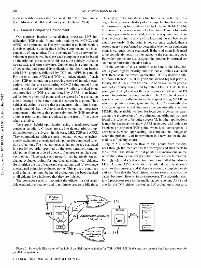
Figure 5 illustrates the flow of trial points from the citi-zens through the mediator to the conveyor and then back tothe citizens. The stream of trial points is asynchronous, in thesense that citizens can always submit points at each iteration.Here Q1, Q2, and Q3 denote trial points submitted by citizensLHS, TGP, and APPS, Q denotes the ordered list of trial pointsgiven to the conveyor, and R denotes recently completed eval-uations. Note that the TGP citizen worker stores a copy of thecache, because it lives on its own processor. This algorithm usesK +2 processors (one for the mediator, conveyor and APPS andone for the TGP citizen worker) and K evaluation processors.

Figure 5. Schematic illustration of the hybrid parallel implementation for TGP–APPS. MPI is the message passing interface, a protocol forparallel computation.


Dow

nloa

ded

by [1

07.1

0.14

8.4]

at 1

2:07

10

Dec

embe

r 201

2


Present implementations of APPS cannot efficiently use morethan 2d + 1 evaluation processors, where d is the dimension ofthe optimization problem; however, extra available processorswill always be useful in evaluating additional points from theTGP generated search pattern. Three processors are the min-imum required for proper execution of the algorithm: one toserve as the mediator, one for APPS, and one for TGP.

3.4 Results for Example Problems

We have recorded the results from 10 optimizations of eachexample function, using stand-alone APPS as well as the hybridTGP–APPS, both with and without an initial LHS of 20 points.Each of these were run on seven of the eight available compu-tation nodes on a Mac Pro with two quad core 3.2-GHz proces-sors. Parameterization of the algorithm follows the directionsdetailed in Sections 2.2 and 3.1, and each TGP-generated searchpattern consists of 20 locations. Except when initial sampling isused to determine a starting location, the initial guess for eachproblem is x = (4,4). To replicate the situation of a relativelyexpensive objective function, a random wait time of 5–10 sec-onds was added to each function evaluation.

Table 1 presents average solutions and numbers of evalua-tions, and Figure 1 shows a selection of traces of xbest plottedover the response surfaces. For the Rosenbrock problem, wesee that APPS entailed a vast increase in computational expenseover TGP–APPS methods and was unable to locate the globalminimum. Thus, in a problem designed to be difficult for localoptimization methods, the hybrid algorithm offers a clear ad-vantage by allowing the search to jump to optimal areas of theinput domain. Conversely, the Shubert function is designed tobe especially problematic for global optimization algorithms.Indeed, we observe that TGP–APPS required more iterationsto locate a minimum than APPS alone. However, the increasein the number of evaluations is much less than would be seenfor a truly global optimization algorithm, such as simulated an-nealing or genetic search. Note that the higher average Shubertsolution for APPS is due only to one particularly poor optimiza-tion in which the pattern search converged on a local minimumof −48.51 after 28 iterations. The potential for such nonopti-mal convergence highlights the advantage of extra robustnessand global scope provided by the hybrid TGP–APPS, with thecost being a doubling of the required function evaluations.

Figure 6 shows an objective function response trace duringTGP–APPS (with initial LHS) optimization of the Rosenbrockand Shubert problems. The Rosenbrock trace plot is particu-larly informative, highlighting a property of TGP–APPS that

Figure 6. Objective function response trace during TGP–APPS op-timization of the Rosenbrock (top) and Shubert (bottom) problems.Black points were generated by the TGP ranking algorithm, and graypoints were generated by the APPS search component.

we have repeatedly observed in practice. In the early part ofthe optimization, where there is much room for improvementover the present best point, the emulator-chosen locations cor-respond to decent response values and are commonly found tobe the next-best point. As the optimization approaches conver-gence, the improvement values are driven entirely by predic-tive uncertainty, leading to a wide search of the input spaceand almost no probability that the next-best point will havebeen proposed by the emulator. For example, in the Rosen-brock optimization, most of iterations 111–130 (correspond-ing to points generated by the TGP ranking algorithm) led toobjective response >2000 (and do not appear on the plot).When this happens, the efficient local optimization of APPSwill drive the optimization, leading to a quick and precise localconvergence. In this way, APPS and TGP each contribute theirstrengths to the project. Indeed, it may be desirable in futureapplications to devise a scheme in which the priority for evalua-tion of TGP-generated locations is downgraded once the poste-rior probability of nonzero improvement reaches some minimallevel.

Table 1. Rosenbrock and Shubert problem results

Method Problem Evaluations Solution

APPS Rosenbrock 13,918.3 (331.7) 0.0664 (0)

APPS–TGP (no LHS) Rosenbrock 965.2 (845.7) 0.0213 (0.0162)

APPS–TGP (with LHS) Rosenbrock 526.9 (869.3) 0.0195 (0.0227)

APPS Shubert 81.2 (18.9) −172.91 (43.7)

APPS–TGP (no LHS) Shubert 206.0 (46.75) −186.73 (0)

APPS–TGP (with LHS) Shubert 180.7 (47.03) −186.73 (0)

NOTE: For each optimization algorithm, the average and standard deviation (in brackets) for the number of function evaluations required and objective response at converged solutionfrom a sample of 10 runs.


Dow

nloa

ded

by [1

07.1

0.14

8.4]

at 1

2:07

10

Dec

embe

r 201

2


4. OPTIMIZATION OF A TRANSISTOR SIMULATOR

We now discuss the optimization problem of calibrating aradiation-aware simulation model for an electrical device com-ponent of a circuit. In this case, the goal of the optimization is tofind appropriate simulator parameter values such that the result-ing simulator output is as close as possible (under the distancefunction defined in (7)) to results from real-world experimentsinvolving the electrical devices of interest. The model input isa radiation pulse expressed as dose rate over time. The corre-sponding output is a curve of current value over time that re-flects the response of the electrical device. The electrical de-vices, both bipolar junction transistors (BJTs), are the bft92 andthe bfs17a. BJTs are widely used in the semiconductor industryto amplify electrical current (refer to Sedra and Smith 1997 orCogdell 1999 for more information), and the two in this studyare particularly common. All BJTs share a basic underlyingmodel, and thus the same computer simulator can be used toapproximate their behavior, with changes only to the tuning pa-rameters required. The real-world data, to which the simulatedcurrent response is compared, consists of six observations atvarious testing facilities. In each experiment, the devices of in-terest are exposed to a unique radiation photocurrent pulse, andthe resulting current behavior is recorded. Additional detailsabout the experiments carried out, the experimental process,and the facilities used have been provided by Gray et al. (2007).It also should be noted that selecting an appropriate subset ofthe real-world data was a problem unto itself, as described byLee, Taddy, and Gray (2008).

The particular simulator of interest is a Xyce implementationof the Tor Fjeldy photocurrent model for the BJT. Xyce is anelectrical circuit simulator developed at Sandia National Labo-ratories (Keiter 2004). The Tor Fjeldy photocurrent model wasdescribed in detail by Fjeldy, Ytterdal, and Shur (1997). Thereare 38 user-defined tuning parameters that determine simulatoroutput for a given radiation pulse input. The objective functionfor optimization is the following measure of distance betweensimulator output and experimental observation of current pathsin time for a set of specific radiation pulse inputs:

f (x) =N∑

i=1

1Ti

Ti∑

t=1

[(Si(t;x) − Ei(t))2]. (7)

Here N = 6 is the number of experiments (each correspond-ing to a unique radiation pulse), Ti is the total number of timeobservations for experiment i, Ei(t) is the amount of electricalcurrent observed during experiment i at time t, and Si(t;x) isthe amount of electrical current at time t as computed by thesimulator with tuning parameters x and radiation pulse corre-sponding to experiment i.

Based on discussions with experimentalists and researchersfamiliar with the simulator, 30 of the tuning parameters werefixed in advance to values either well known in the semiconduc-tor industry or determined through analysis of the device con-struction. The semiconductor engineers also provided boundsfor the remaining eight parameters, our objective function in-put x. This parameter set includes those believed to have both alarge overall effect on the output of the model and a high levelof uncertainty with respect to their ideal values. The most un-certain parameters in the radiation-aware model are those that

Figure 7. Sensitivity analysis for bft92 (top) and bfs17a (bottom)devices, based on a TGP fit to an LHS of 160 initial locations, sum-marized by first-order sensitivity indexes (left) and total sensitivity in-dexes (right).

directly affect the amount of radiation collected, and these eightparameters are all part of the device doping profile. The dopingprocess introduces impurities to change the electrical propertiesof the device, and the amount of doping will affect the amountof photocurrent collected by the device. Four of the parameters(x1, x2, x3, x4) describe the lightly doped collector, whereas theother four (x5, x6, x7, x8) describe the heavily doped collector.Figure 7 shows the results of an MCMC sensitivity analysis, asdescribed in Section 3.2, based on a TGP model fit to an initialLHS of 160 input locations and with respect to a uniform uncer-tainty distribution over the bounded parameter space. Becausethe mean total effect indexes are all >0.1, we decided that fur-ther reduction of the problem dimension was impossible. Wenote that, as indicated by the difference between first-order andtotal sensitivity indexes, some variables are influential only ininteraction with the other inputs.

The objective of (7) was optimized using both APPS and thehybrid algorithm TGP–APPS. The problems were initiated withthe same starting values, the best guess provided by the semi-conductor engineer, and were run on a cluster using eight com-pute nodes with dual 3.06-GHz Intel Xenon processors with2 GB of RAM. In the case of the hybrid algorithm, initial LHSsof 160 points were used to inform the TGP. All LHS designsare taken with respect to independent uniform distributions overthe bounded input space. The wall clock time and the numberof objective function evaluations corresponding to each deviceand each optimization algorithm are given in Table 2. Figure 8shows simulated current response curves corresponding to eachsolution and to the initial guess for tuning parameter values, aswell as the data, for a single radiation pulse input to each de-vice. The initial guess represents the best values known to theexperimentalists before the optimization was done. The resultsfor the other radiation pulse input values exhibit similar proper-ties.


Dow

nloa

ded

by [1

07.1

0.14

8.4]

at 1

2:07

10

Dec

embe

r 201

2


Table 2. The number of objective function evaluations, total wall clock time required to find a solution, and the optimized objective responsefor each BJT device and each optimization algorithm

Method Device Evaluations Time Objective

APPS bft92 6,823 341,257 sec ≈ 95 hrs 2.01644e−2APPS–TGP bft92 962 49,744 sec ≈ 14 hrs 2.01629e−2APPS bfs17a 811 37,038 sec ≈ 10 hrs 3.22625e−2APPS–TGP bfs17a 1389 65,122 sec ≈ 18 hrs 2.73194e−2

In the case of bft92, the solutions produced by the two op-timization algorithms are practically indistinguishable. But theAPPS solution was obtained only after a huge additional com-putational expense, illustrating the ability of the hybrid algo-rithm to move the search pattern quickly into decent areas ofthe input space. We note that a similarly low computational time(56,815 seconds ≈ 16 hours) was required to obtain an equiv-alent solution using TGP–APPS without the initial sampling(i.e., starting from the same parameter vector as for APPS).

For the bfs17a, the difference in the resulting response curvesis striking and illustrates the desirable robustness of our hybridalgorithm. The response curve created using the parameter val-ues obtained by APPS alone differs significantly from the datain overall shape. In contrast, the curve resulting from the pa-rameters found by TGP–APPS is a better match to the experi-mental data. These results suggest that the APPS algorithm wasunable to overcome a weak local minimum, whereas the inclu-sion of TGP allowed for a more comprehensive search of thedesign space. Overall, the APPS–TGP required more computa-tional resources to find a solution; however, because of the poorquality of the APPS solution, the optimization would have hadto be rerun using different starting points until a more optimalsolution could be found, with the computational cost quicklysurpassing that of TGP–APPS. Thus the extra computationalcost of TGP–APPS is well justified by the improvement in fitand the ability to find a robust solution with just one startingpoint.

Table 3 gives the converged optimal parameterization foreach device through the use of each of APPS and TGP–APPS

Figure 8. Simulated response current curves, corresponding todifferent tuning parameter values, for the bft92 (left) and bfs17a(right) devices. The solid line represents the response for parametersfound using TGP–APPS, the dashed line represents parameters foundthrough APPS alone, and the dotted line represents the initial para-meter vector guess. The experimental current response curves for theradiation impulse used in these simulations are shown in gray.

with an LHS initial sample. As illustrated in Figure 8, a perfectsolution was unobtainable. The lack of fit can be attributed inpart to a disconnect between the actual and simulated radiationpulses; a prespecified pulse apparently tends to be larger thanexpected in the laboratory, leading to a muted simulation re-sponse curve for equivalent doses. This situation also may haveled to incorrect bounds on the potential input domain. Nonethe-less, both the modelers and experimentalists were pleased withthe improved fit provided by TGP–APPS. In fact, for this real-world problem, the solutions presented herein are the bestknown to date. A complete statistical calibration of this sim-ulator would require the modeling of a bias term, as in the workof Kennedy and O’Hagan (2001); however, in the context ofoptimum control, we are confident that these results providea robust solution with respect to minimization of the providedobjective function. Indeed, the robustness of TGP–APPS allowsmodelers to be confident that these solutions are practically asclose as possible to the true current response curves. This dis-covery has convinced Sandia that the issues underlying theseinadequacies in the simulator model merit future study.

5. CONCLUSION

We have described a novel algorithm for statistically guidedpattern search. Along with the general optimization methodol-ogy described in Sections 3.2 and 3.3, we outline a powerfulframework that uses the strengths of both statistical inferenceand pattern search. The general hybridization scheme, as wellas the algorithm for statistically ranking candidate locations,do not require the use of APPS or TGP specifically and can beimplemented in conjunction with alternative local search or sta-tistical emulation approaches. Thus our methodology providesa general framework for statistically robust local optimization.Our algorithm will almost always lead to a more robust solutionthan that obtained through local pattern search, and we havealso observed that it can provide faster optimization in prob-lems that are difficult for local methods.

Although we have focused on deterministic objective func-tions, the optimization algorithm is directly applicable to opti-mization in the presence of random error. Changes to the nuggetparameter prior specification are all that are required for TGP tomodel noisy data, and APPS adapts for observation error by in-creasing the tolerance δ in the sufficient decrease criterion (seeSec. 2.1). Because the primary stopping criterion is based onstep length, and because step length decreases with each searchthat does not produce a new best point, δ ensures that evalua-tions are not wasted on optimizing noise.

An appealing aspect of any oracle scheme is that becausepoints are given in addition to those generated by the pattern


Dow

nloa

ded

by [1

07.1

0.14

8.4]

at 1

2:07

10

Dec

embe

r 201

2


Table 3. Initial guesses and final solutions for bft92 and bfs17a simulator parameters

bft92 Initial APPS TGP–APPS bfs17a Initial APPS TGP–APPS

x1 5e−3 3.55e−3 3.55e−3 x1 5e−3 3.55e−3 3.55e−3x2 1.4e−3 1.08e−3 1.30e−3 x2 1.4e−3 1.30e−3 1.30e−3x3 1e−8 1.00e−9 1.00e−9 x3 1e−6 1.00e−6 1.00e−9x4 2e−8 6.15e−8 6.40e−8 x4 2e−6 1.00e−5 1.00e−5x5 4e−3 3.55e−3 2.63e−3 x5 4e−3 3.55e−3 3.55e−3x6 1.6e−3 1.30e−3 1.30e−3 x6 1.6e−3 1.30e−3 1.20e−3x7 1e−9 1.61e−7 2.17e−7 x7 1e−7 1.00e−5 1.19e−6x8 2e−9 1.00e−5 1.00e−5 x8 2e−7 2.00e−7 1.00e−5

search, there is no adverse affect on the local convergence. Inthe setting of robust optimization, either with or without ob-servation error, there are two additional major criteria for as-sessing convergence. First, the converged solution should notlie on a knifes edge portion of the response surface. Second, theresponse at this solution needs to be close to the global opti-mum. In each case, the statistical emulator provides guidanceas to the acceptability of any converged solution. Informally,the mean predictive surface allows the optimizer to judge theshape of the response around the solution and the magnitudeof the optimum with respect to other potential optima aroundthe input space. Moreover, the full accounting of TGP uncer-tainty provides a measure of the level of confidence that maybe placed in this predicted surface. Formally, quantiles of pre-dicted improvement provide a precise measure of the risk of asignificantly better alternate optimum at unobserved locations;for example, a 95th percentile for improvement I(x) that is zeroover the input domain would support a claim that the convergedsolution corresponds to a global optima. Future work in thisdirection could lead to substantial contributions in applied op-timization.

[Received January 2008. Revised October 2008.]

REFERENCES

Alexandrov, N., Dennis, J. E., Lewis, R. M., and Torczon, V. (1998), “A TrustRegion Framework for Managing the Use of Approximation Models in Op-timization,” Structural Optimization, 15, 16–23.

Booker, A. J., Dennis, J. E., Frank, P. D., Serafini, D. B., Torczon, V., and Tros-set, M. W. (1999), “A Rigorous Framework for Optimization of ExpensiveFunctions by Surrogates,” Structural and Multidisciplinary Optimization,17, 1–13.

Chipman, H., George, E., and McCulloch, R. (1998), “Bayesian CART ModelSearch” (with discussion), Journal of the American Statistical Association,93, 935–960.

(2002), “Bayesian Treed Models,” Machine Learning, 48, 303–324.Cogdell, J. R. (1999), Foundations of Electronics, Upper Saddle River, NJ:

Prentice Hall.Currin, C., Mitchell, T., Morris, M., and Ylvisaker, D. (1991), “Bayesian Pre-

diction of Deterministic Functions, With Applications to the Design andAnalysis of Computer Experiments,” Journal of the American StatisticalAssociation, 86, 953–963.

Fang, K.-T., Li, R., and Sudjianto, A. (2006), Design and Modeling for Com-puter Experiments, Boca Raton: Chapman & Hall/CRC.

Fjeldy, T. A., Ytterdal, T., and Shur, M. S. (1997), Introduction to Device Mod-eling and Circuit Simulation, Hoboken, NJ: Wiley.

Fowler, K. R., Reese, J. P., Kees, C. E., Dennis, J. E., Jr., Kelley, C. T., Miller,C. T., Audet, C., Booker, A. J., Couture, G., Darwin, R. W., Farthing, M. W.,Finkel, D. E., Goblansky, J. M., Gray, G. A., and Kolda, T. G. (2008),“A Comparison of Derivative-Free Optimization Methods for Water Sup-ply and Hydraulic Capture Community Problems,” Advances in Water Re-sources, 31, 743–757.

Gramacy, R. B. (2007), “tgp: An R Package for Bayesian Nonstationary, Semi-parametric Nonlinear Regression and Design by Treed Gaussian ProcessModels,” Journal of Statistical Software, 19 (9).

Gramacy, R. B., and Lee, H. K. H. (2008), “Bayesian Treed Gaussian ProcessModels With an Application to Computer Modeling,” Journal of the Amer-ican Statistical Association, 103, 1119–1130.

Gray, G. A., and Kolda, T. G. (2006), “Algorithm 856: APPSPACK 4.0: Asyn-chronous Parallel Pattern Search for Derivative-Free Optimization,” ACMTransactions on Mathematical Software, 32 (3), 485–507.

Gray, G. A. et al. (2007), “Designing Dedicated Experiments to Support Val-idation and Calibration Activities for the Qualification of Weapons Elec-tronics,” in Proceedings of the 14th NECDC. Also available as TechnicalReport SAND2007-0553C, Sandia National Laboratories.

Green, P. (1995), “Reversible Jump Markov Chain Monte Carlo Computationand Bayesian Model Determination,” Biometrika, 82, 711–732.

Hedar, A.-R., and Fukushima, M. (2006), “Tabu Search Directed by DirectSearch Methods for Nonlinear Global Optimization,” European Journal ofOperational Research, 127 (2), 329–349.

Higdon, D., Kennedy, M., Cavendish, J., Cafeo, J., and Ryne, R. (2004), “Com-bining Field Data and Computer Simulations for Calibration and Predic-tion,” SIAM Journal of Scientific Computing, 26, 448–466.

Jones, D., Schonlau, M., and Welch, W. (1998), “Efficient Global Optimizationof Expensive Black-Box Functions,” Journal of Global Optimization, 13,455–492.

Keiter, E. R. (2004), “Xyce Parallel Elctronic Simulator Design: MathematicalFormulation,” Technical Report SAND2004-2283, Sandia National Labo-ratories.

Kennedy, M., and O’Hagan, A. (2001), “Bayesian Calibration of ComputerModels,” Journal of the Royal Statistical Society, Ser. B, 63, 425–464.

Kolda, T. G. (2005), “Revisiting Asynchronous Parallel Pattern Search for Non-linear Optimization,” SIAM Journal on Optimization, 16 (2), 563–586.

Kolda, T. G., Lewis, R. M., and Torczon, V. (2003), “Optimization by DirectSearch: New Perspectives on Some Classical and Modern Methods,” SIAMReview, 45, 385–482.

(2006), “Stationarity Results for Generating Set Search for LinearlyConstrained Optimization,” SIAM Journal on Optimization, 17 (4), 943–968.

Lee, H. K. H., Taddy, M., and Gray, G. A. (2008), “Selection of a Represen-tative Sample,” Technical Report UCSC-SOE-08-12, University of Califor-nia, Santa Cruz, Department of Applied Mathematics and Statistics. Alsoavailable as Report SAND2008-3857J, Sandia National Laboratories.

McKay, M., Beckman, R., and Conover, W. (1979), “A Comparison of ThreeMethods for Selecting Values of Input Variables in Analysis of Output Froma Computer Code,” Technometrics, 21, 239–245.

Mease, D., and Bingham, D. (2006), “Latin Hyperrectangle Sampling for Com-puter Experiments,” Technometrics, 48, 467–477.

Morris, R. D., Kottas, A., Taddy, M., Furfaro, R., and Ganapol, B. (2008),“A Statistical Framework for the Sensitivity Analysis of Radiative Trans-fer Models,” IEEE Transactions on Geoscience and Remote Sensing, 12,4062–4074.

Oakley, J., and O’Hagan, A. (2004), “Probabilistic Sensitivity Analysis of Com-plex Models: A Bayesian Approach,” Journal of the Royal Statistical Soci-ety, Ser. B, 66, 751–769.

O’Hagan, A., Kennedy, M. C., and Oakley, J. E. (1998), “Uncertainty Analysisand Other Inference Tools for Complex Computer Codes,” in Bayesian Sta-tistics 6, eds. J. M. Bernardo, J. O. Berger, A. P. Dawid, and A. F. M. Smith,Oxford, U.K.: Oxford University Press, pp. 503–524.

Regis, R. G., and Shoemaker, C. A. (2007), “Improved Strategies for RadialBasis Function Methods for Global Optimization,” Journal of Global Opti-mization, 37 (1), 113–135.

Sacks, J., Welch, W., Mitchell, T., and Wynn, H. (1989), “Design and Analysisof Computer Experiments,” Statistical Science, 4, 409–435.


Dow

nloa

ded

by [1

07.1

0.14

8.4]

at 1

2:07

10

Dec

embe

r 201

2


Saltelli, A. (2002), “Making Best Use of Model Evaluations to Compute Sen-sitivity Indices,” Computer Physics Communications, 145, 280–297.

Saltelli, A., Chan, K., and Scott, E. (eds.) (2000), Sensitivity Analysis, Hoboken,NJ: Wiley.

Saltelli, A., Ratto, M., Andres, T., Campolongo, F., Cariboni, J., Gatelli, D.,Saisana, M., and Tarantola, S. (2008), Global Sensitivity Analysis: ThePrimer, Hoboken, NJ: Wiley.

Santner, T., Williams, B., and Notz, W. (2003), The Design and Analysis ofComputer Experiments, New York: Springer-Verlag.

Schonlau, M., Welch, W., and Jones, D. (1998), “Global versus Local Search inConstrained Optimization of Computer Models,” in New Developments andApplications in Experimental Design. IMS Lecture Notes, eds. N. Flournoy,

W. F. Rosenberger, and W. K. Wong, Bethesda, MD: Institute of Mathemat-ical Statistics, pp. 11–25.

Sedra, A. S., and Smith, K. C. (1997), Microelectronic Circuits (4th ed.), Ox-ford, U.K.: Oxford University Press.

Stein, M. (1987), “Large Sample Properties of Simulations Using Latin Hyper-cube Sampling,” Technometrics, 29, 143–151.

Wright, M. H. (1996), “Direct Search Methods: Once Scorned, Now Re-spectable,” in Numerical Analysis 1995 (Proceedings of the 1995 DundeeBiennial Conference in Numerical Analysis), eds. D. F. Griffiths andG. A. Watson. Pitman Research Notes in Mathematics, Vol. 344, Essex,U.K.: Addison-Wesley, pp. 191–208.


Dow

nloa

ded

by [1

07.1

0.14

8.4]

at 1

2:07

10

Dec

embe

r 201

2

Documents

Bayesian Guided Pattern Search for Robust Local Optimization