Bayesian Confidence Limits and Intervals - Stanford … · SLUO Statistics Lectures 2006 Bayesian Confidence Intervals Slide 3 This is Subjective (Bayesian) probability GOOD I can

Bayesian Confidence Limits and Intervals

Roger BarlowSLUO Lectures on Statistics

August 2006

SLUO Statistics Lectures 2006

Bayesian Confidence Intervals Slide 2

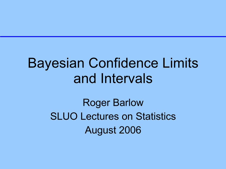
Probability RevisitedI say:“The probability of rain tomorrow is 70%”I mean:I regard 'rain tomorrow' and 'drawing a white

ball from an urn containing 7 white balls and 3 black balls' as equally likely.

By which I mean:If I were offered a choice of betting on one or

the other, I would be indifferent.



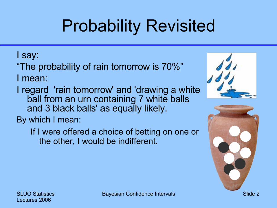
This is Subjective (Bayesian) probability

GOODI can talk about – and do

calculations on – the probability of anything:

• Tomorrow's weather • The Big Bang• The Higgs mass• The existence of God• The age of the current

king of France

BADThere is no reason for my

probability values to be the same as your probability values

I may use these probabilities for my own decisions, but there is no call for me to impose them on others



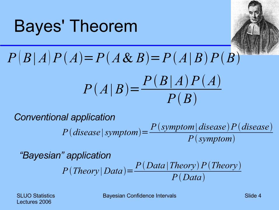
Bayes' Theorem

P B | A P A=P A& B=P A | BP B

P A | B= P B | AP AP B

Conventional application

“Bayesian” application

P disease | symptom= P symptom | diseaseP diseaseP symptom

P Theory | Data =P Data |TheoryP Theory P Data



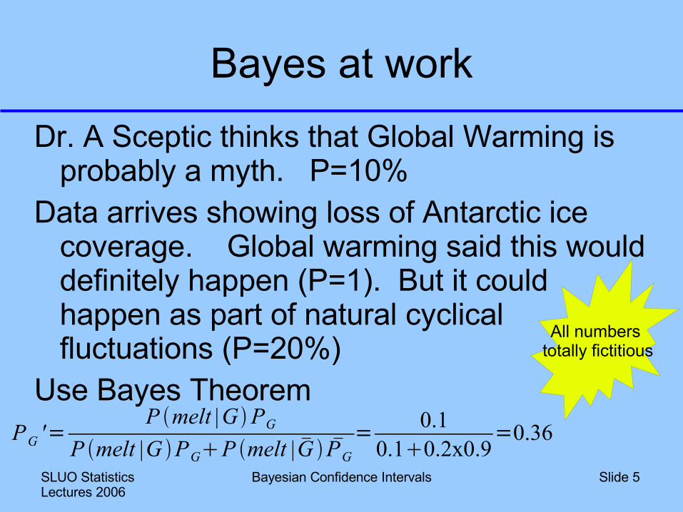
Bayes at workDr. A Sceptic thinks that Global Warming is

probably a myth. P=10%Data arrives showing loss of Antarctic ice

coverage. Global warming said this would definitely happen (P=1). But it could happen as part of natural cyclical fluctuations (P=20%)

Use Bayes TheoremPG '=

P melt |GPG

P melt |G PGP melt | G PG= 0.1

0.10.2x0.9=0.36

All numbers totally fictitious



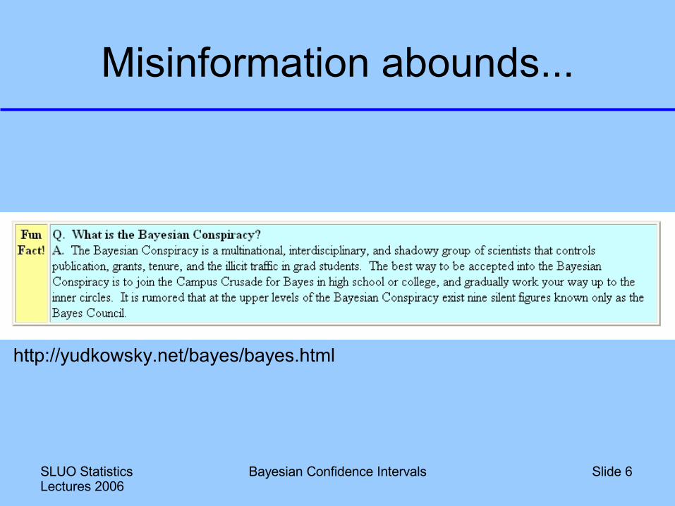
Misinformation abounds...

http://yudkowsky.net/bayes/bayes.html



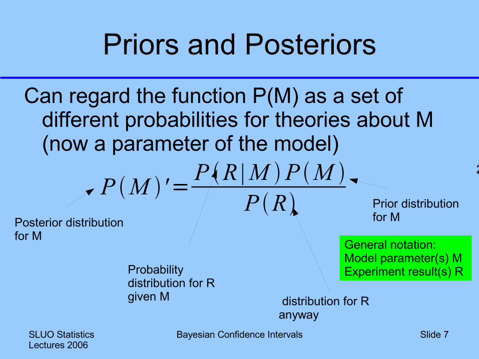
Priors and PosteriorsCan regard the function P(M) as a set of

different probabilities for theories about M (now a parameter of the model)

P M '= P R | M P M P R Prior distribution

for MPosterior distribution for M

2.302.30

Probability distribution for R given M distribution for R

anyway

General notation:Model parameter(s) MExperiment result(s) R



Probability and The Likelihood Function

P(R|M) is the probability of what can be a a whole set of results R, as a function of the model parameter(s) M

Also known as the likelihood L(R,M)It is always tempting to think of it as L(M,R): Probability

for model parameter(s) M given result(s) RFor frequentists this is rubbish. For Bayesians it follows

if the prior is uniform.



'Inverse Probability'Bayes theorem says:

P(M|R) ∝ P(R|M)Call this 'inverse probability'. Probability distribution for

a model parameter M given a result R. Just normaliseSeems easy.But:P(M) is meaningless/nonexistent in frequentist

probabilityWorking with P(M) and P(M2) and P(ln M) will give

different and incompatible answers



Integrating the Likelihood function L(R,M)

For Bayesians:Go ahead.Be aware that if you

reparametrise M then your results will change

Unless you specify a prior and reparametrise that

For Frequentists, integrating L wrt M is unthinkable.

Integrating/summing over R is fine. Use it to get expectation values

If you integrate a likelihood then you're doing something Bayesian. If you are a Bayesian, this is not a problem.If you claim to be a frequentist, you have crossed a borderline somewhere



Uniform prior

• Often take P(M) as constant (“flat prior”)• Strictly speaking P(M) should be

normalised: ∫P(M) dM =1• Over an infinite range this makes the

constant zero...• Never mind! Call it an “Improper Prior” and

normalise the posterior• A prior flat in M is not flat in M' (ln M, M2, ..)



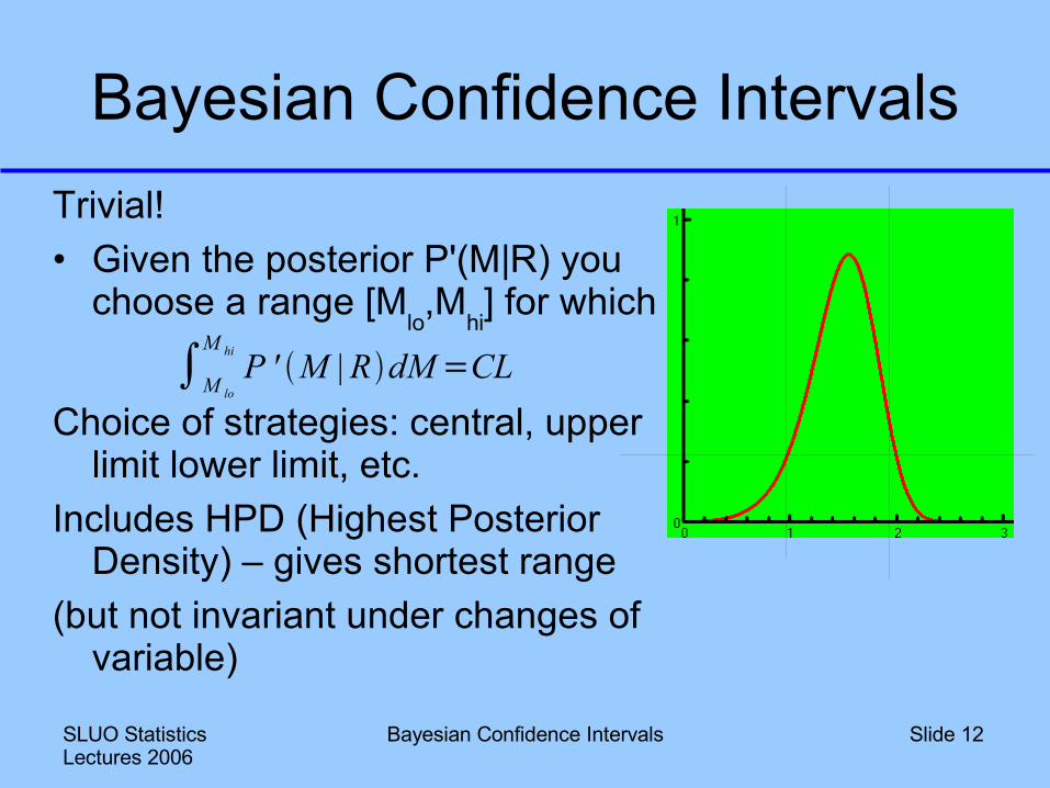
Bayesian Confidence IntervalsTrivial!• Given the posterior P'(M|R) you

choose a range [Mlo,M

hi] for which

Choice of strategies: central, upper limit lower limit, etc.

Includes HPD (Highest Posterior Density) – gives shortest range

(but not invariant under changes of variable)

∫M lo

M hi P ' M | RdM =CL



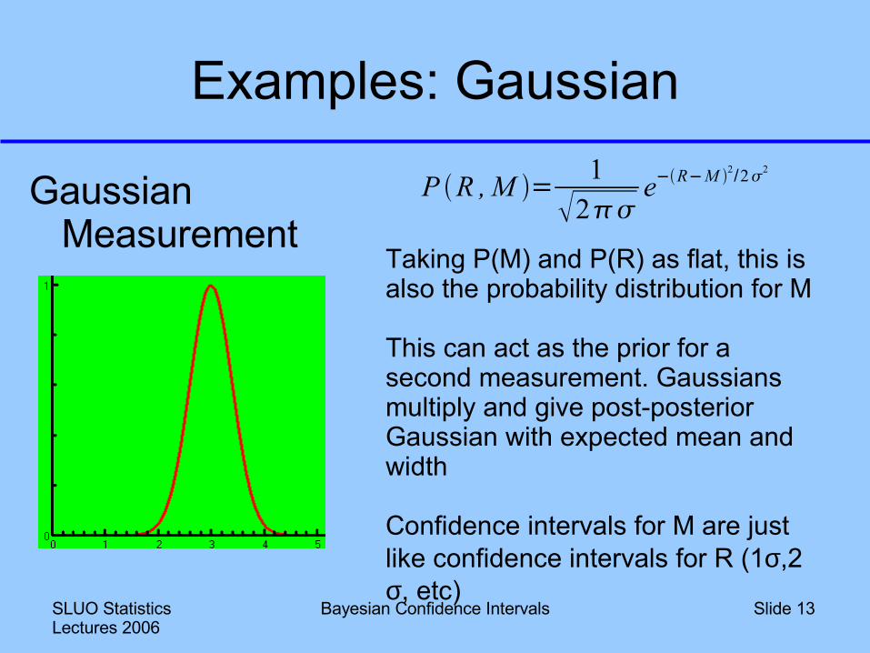
Examples: Gaussian

Gaussian Measurement

P R , M = 12

e−R−M 2/22

Taking P(M) and P(R) as flat, this is also the probability distribution for M

This can act as the prior for a second measurement. Gaussians multiply and give post-posterior Gaussian with expected mean and width

Confidence intervals for M are just like confidence intervals for R (1σ,2σ, etc)



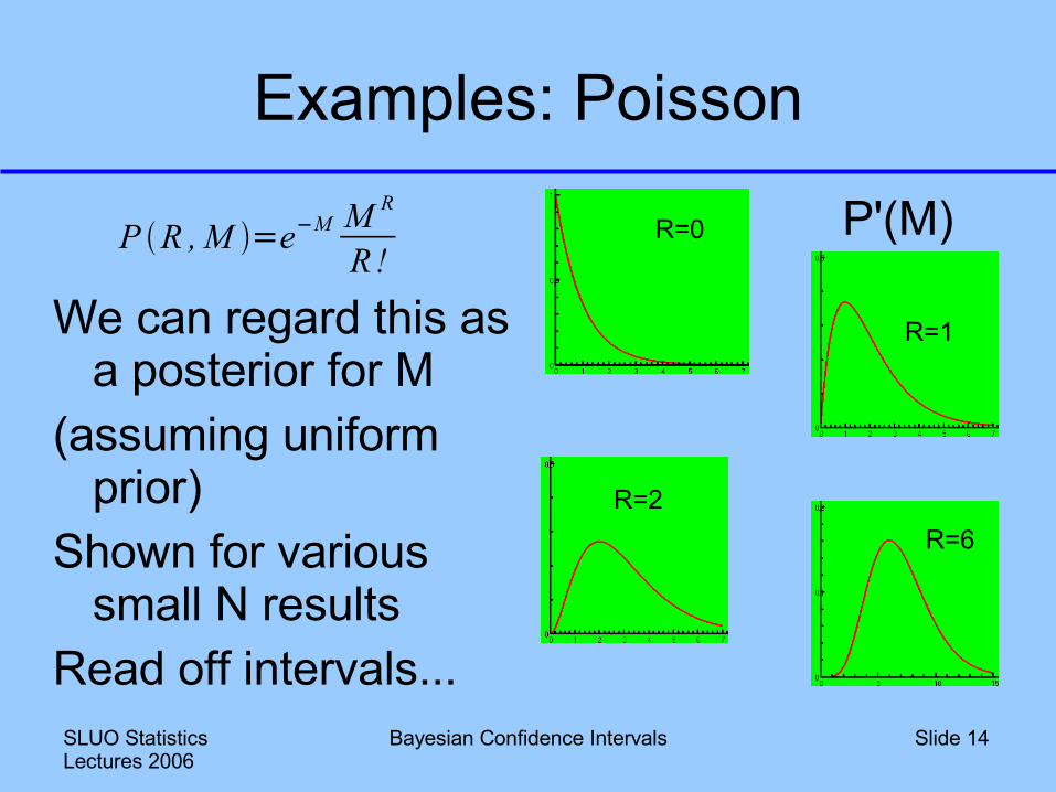
Examples: Poisson

We can regard this as a posterior for M

(assuming uniform prior)

Shown for various small N results

Read off intervals...

P R , M =e−M M R

R!

R=6R=2

R=1

R=0 P'(M)



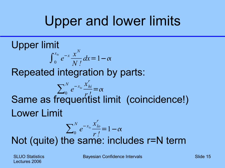
Upper and lower limitsUpper limit

Repeated integration by parts:

Same as frequentist limit (coincidence!)Lower Limit

Not (quite) the same: includes r=N term

∫0

xhi

e−x xN

N !dx=1−

∑0

Ne−xlo

x lor

r !=1−

∑0

Ne−xhi

xhir

r !=



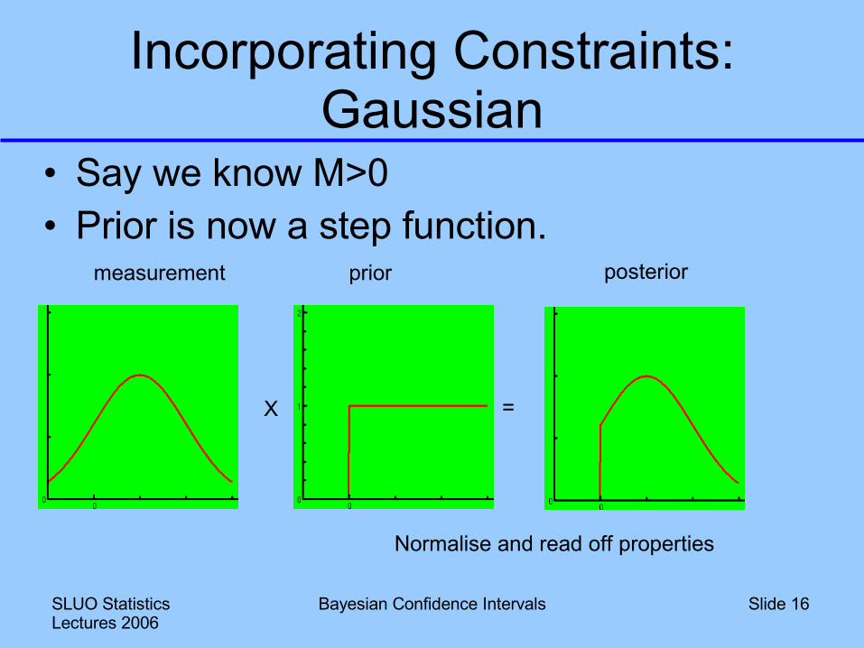
Incorporating Constraints: Gaussian

• Say we know M>0• Prior is now a step function.

X =

measurement posteriorprior

Normalise and read off properties



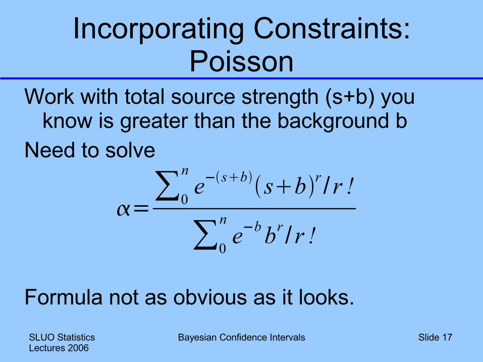
Incorporating Constraints: Poisson

Work with total source strength (s+b) you know is greater than the background b

Need to solve

Formula not as obvious as it looks.

=∑0

ne−sbsbr / r !

∑0

ne−b br / r !



Robustness

• Result depends on chosen prior• More data reduces this dependence • Statistical good practice: try several priors

and look at the variation in the result• If this variation is small, result is robust

under changes of prior and is believable• If this variation is large, it's telling you the

result is meaningless



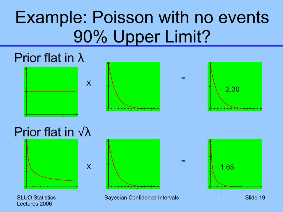
Example: Poisson with no events90% Upper Limit?

Prior flat in λ

Prior flat in √λ

X

X=

=1.65

2.30



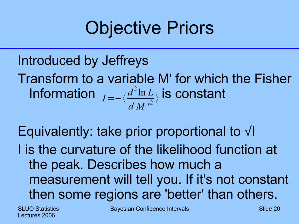
Objective Priors

Introduced by JeffreysTransform to a variable M' for which the Fisher

Information is constant

Equivalently: take prior proportional to √II is the curvature of the likelihood function at

the peak. Describes how much a measurement will tell you. If it's not constant then some regions are 'better' than others.

I=−⟨ d 2 ln Ld M ' 2 ⟩

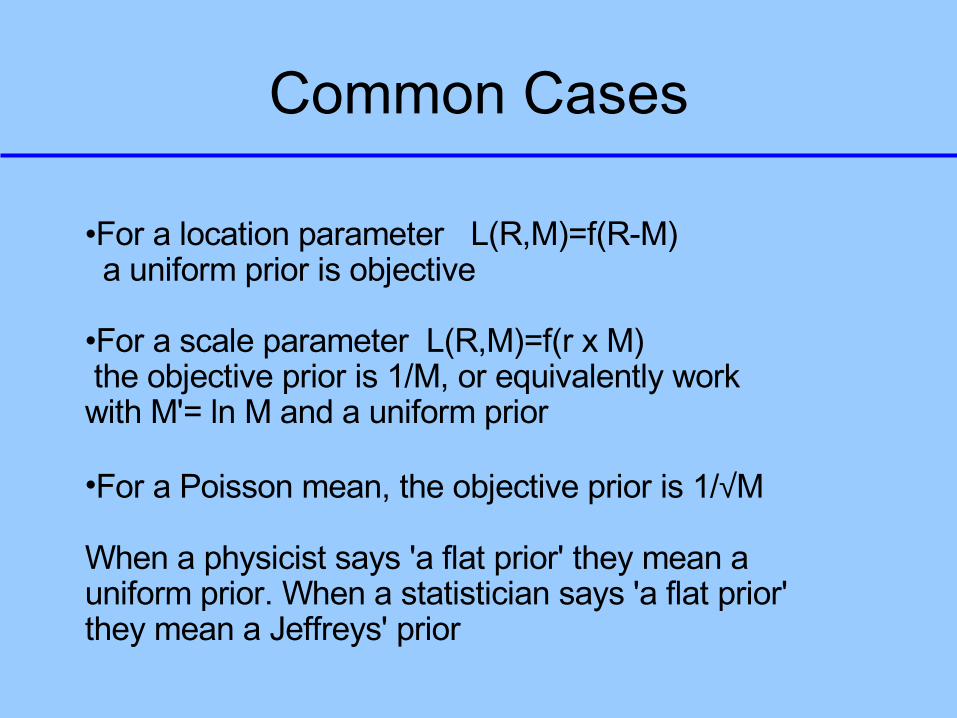
Common Cases

•For a location parameter L(R,M)=f(R-M) a uniform prior is objective

•For a scale parameter L(R,M)=f(r x M) the objective prior is 1/M, or equivalently work with M'= ln M and a uniform prior

•For a Poisson mean, the objective prior is 1/√M

When a physicist says 'a flat prior' they mean a uniform prior. When a statistician says 'a flat prior' they mean a Jeffreys' prior

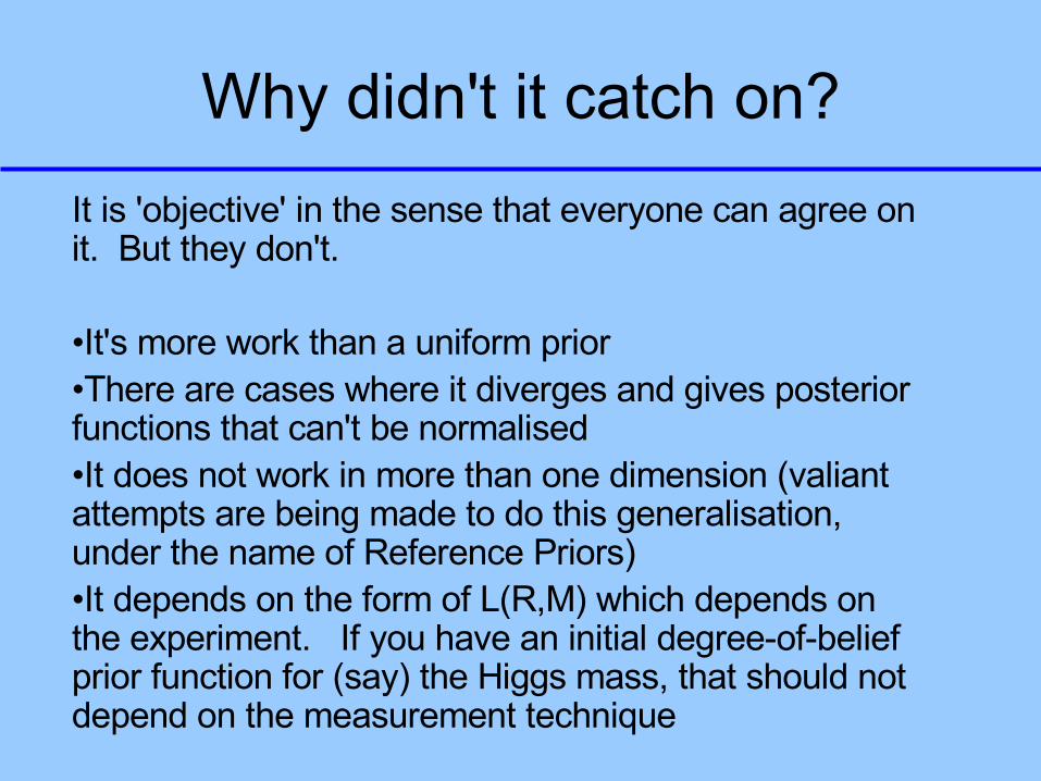
Why didn't it catch on?It is 'objective' in the sense that everyone can agree on it. But they don't.

•It's more work than a uniform prior•There are cases where it diverges and gives posterior functions that can't be normalised•It does not work in more than one dimension (valiant attempts are being made to do this generalisation, under the name of Reference Priors)•It depends on the form of L(R,M) which depends on the experiment. If you have an initial degree-of-belief prior function for (say) the Higgs mass, that should not depend on the measurement technique



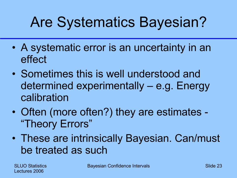
Are Systematics Bayesian?

• A systematic error is an uncertainty in an effect

• Sometimes this is well understood and determined experimentally – e.g. Energy calibration

• Often (more often?) they are estimates - “Theory Errors”

• These are intrinsically Bayesian. Can/must be treated as such



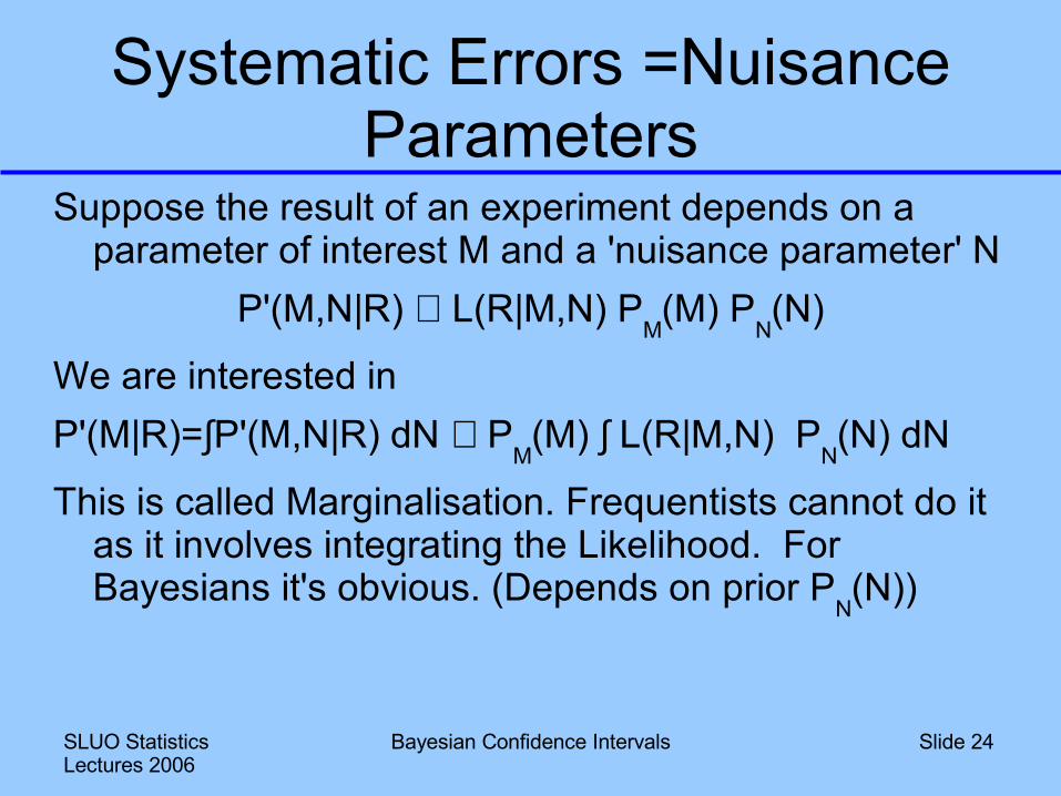
Systematic Errors =Nuisance Parameters

Suppose the result of an experiment depends on a parameter of interest M and a 'nuisance parameter' N

P'(M,N|R) ∝ L(R|M,N) PM(M) P

N(N)

We are interested in P'(M|R)=∫P'(M,N|R) dN ∝ P

M(M) ∫ L(R|M,N) P

N(N) dN

This is called Marginalisation. Frequentists cannot do it as it involves integrating the Likelihood. For Bayesians it's obvious. (Depends on prior P

N(N))



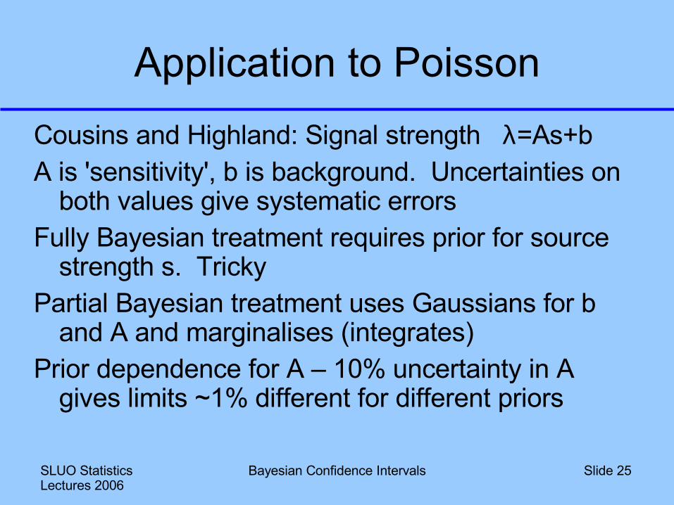
Application to PoissonCousins and Highland: Signal strength λ=As+bA is 'sensitivity', b is background. Uncertainties on

both values give systematic errorsFully Bayesian treatment requires prior for source

strength s. TrickyPartial Bayesian treatment uses Gaussians for b

and A and marginalises (integrates)Prior dependence for A – 10% uncertainty in A

gives limits ~1% different for different priors



Example – CKM fitterLe Diberder, T'Jampens and others

Sad StoryFitting CKM angle α from B→ρρ6 observables3 amplitudes: 6 unknown parameters (magnitudes,

phases) α is the fundamentally interesting one



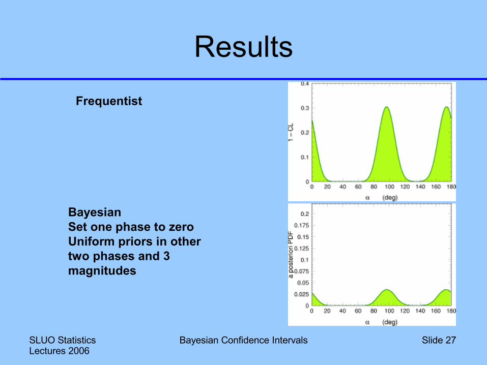
ResultsFrequentist

BayesianSet one phase to zeroUniform priors in other two phases and 3 magnitudes



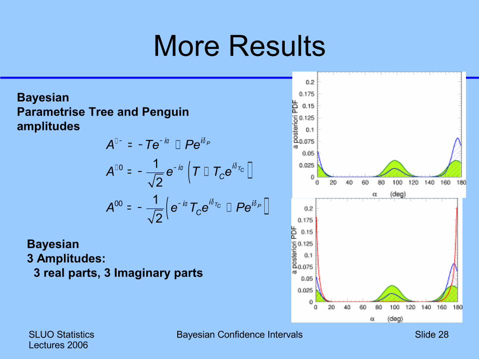
More ResultsBayesianParametrise Tree and Penguin amplitudes

( )( )

0

00

12

12

P

TC

TC P

ii

iiC

i iiC

A Te Pe

A e T T e

A e T e Pe

δα

δα

δ δα

+ − −

+ −

−

= − +

= − +

= − +

Bayesian3 Amplitudes: 3 real parts, 3 Imaginary parts



Interpretation● B→ππ shows same

(mis)behaviour● Removing all experimental

info gives similar P(α)● The curse of high

dimensions is at work

Uniformity in x,y,z makes P(r) peak at large rThis result is not robust

under changes of prior



ConclusionsBayesian Statistics are• Illuminating• Occasionally the only tool to use• Not the answer to everything• To be used with care • Based on shaky foundations ('house built on sand')• Results depend on choice of prior/choice of

variableAlways check for robustness by trying a few different

priors. Serious statisticians do.

Documents

Bayesian Confidence Limits and Intervals - Stanford … · SLUO Statistics Lectures 2006 Bayesian Confidence Intervals Slide 3 This is Subjective (Bayesian) probability GOOD I can