1

Battery Power Smoothing Control in a MarineElectric Power Plant using Nonlinear Model

Predictive ControlTorstein Ingebrigtsen Bø, Member, IEEE, Tor Arne Johansen, Member, IEEE,

Abstract—This paper presents a power variation smoothingmethod using batteries on a weak ship grid. For some marinevessels, power fluctuations on the ac grid are large. This resultsin large variations in the electrical frequency of the grid andexcessive wear and tear of the power producers. Adding batteriesconnected to a DC/AC drive to smooth out the power fluctuationshas been suggested. However, due to the large amount offluctuation, batteries can overheat. Therefore, we suggest usinga band-pass filter with cutoff frequency parameters optimizedby model predictive control based on a power spectral densityestimate of power consumption for disturbance prediction.

Index Terms—Battery management systems, Statistical analy-sis, Optimal control, Stochastic Model Predictive Control, Tem-perature control.

I. INTRODUCTION

Marine vessels with diesel-electric power plants and propul-sion have a weak ac grid, due to the large size of the consumerscompared with the size and number of producers. Therefore,a typical load change will induce voltage and frequencyvariations. On some marine vessels, the power consumptionfluctuates heavily in certain operational and environmentalconditions. Due to the weak grid, this induces fluctuationsin electrical frequency, excessive wear and tear on the powerproducers, and synchronization problems when connecting anew generator set to the grid. Currently, this problem is solvedby connecting additional generators, which gives a stiffer grid.This reduces the efficiency of the plant and increases the needfor maintenance.

The power fluctuations on a vessel may come from heave-compensators, auxiliary systems, wave-induced thruster dis-turbance, rapid changing thrust losses due to ventilation andthruster-thruster interaction, and hotel loads. The period typi-cally varies from 0.1 seconds to hundreds of seconds. Dieselengines prefer to have as constant a load as possible, sincethis reduces thermal stress due to temperature changes. In theauthors experience, diesel engines are not able to compensatefor loads with dynamics faster than about 5-10 seconds due to

T.I. Bø and T.A. Johansen are with center for autonomous marine operationsand systems (NTNU AMOS), Department of Engineering Cybernetics, NTNU- Norwegian University of Science and Technology, 7491, Trondheim, Norway(e-mail: torstein.bo@itk.ntnu.no).

The authors of this paper are funded by the project design to verificationof control systems for safe and energy efficient vessels with hybrid powerplants (D2V), where the Research Council of Norway is the main sponsor.NFR: 210670/070, 223254/F50.

This work was also partly supported by the Research Council of Norwaythrough the Center of Excellence funding scheme, project number 223254 -NTNU AMOS

the turbo-lag. On the other hand, the inertia of the generatorset can compensate for some load fluctuations. Typically, theinertia can handle dynamics faster than 1-3 seconds. However,this increases the mechanical stress on the generator set. Ona marine vessel, the total produced power can be measured atthe generators. This is often done every 0.1 second. Therefore,a power smoothing algorithm should be able to handle fluctu-ations with periods from 0.1 to 100 seconds, but particularlywhere it is most important to take care of loads fluctuationsi.e., periods between 1 and 10 seconds.

Several methods to reduce power fluctuations on marine ves-sels have already been proposed. Using the thruster allocationand feedforward in the governor to reduce power fluctuationshas been proposed in [1], [2]. Another approach was to use thethrusters directly for power smoothing by generating a thrusterload which counteracts other load variations [3], [4]. Typically,thruster biasing is used on vessels with dynamic positioningsystems to reduce load variations; thrusters counteract eachother to waste power, so that other load variations are canceledout [5].

Recently, adding batteries to the grid has been suggested.M/S Viking Queen will soon be retrofitted with batteries [6],while M/S Ampere is in operation and is driven by batteriesonly [7]. Using batteries on naval vessels to take care ofpulse loads from the weapons system has been suggested [8],[9]. Batteries can also be used for emergency power, asdemonstrated in [10]. In this article, batteries are used forpower smoothing. Batteries compensate for the variations inpower consumption, while the generator sets produce slowlyvarying power to meet the demand. The batteries used forthis task must be able to charge and discharge large currents.However, since the mean current is zero, the storage capacitycan be small. One problem with such a large charge anddischarge current is that this produces heat. This heat pro-duction must be controlled or the batteries may disconnectdue to overheating. On some vessels, batteries can be used foremergency power, this requires a larger battery, which is lessprone to heat challenges. Battery power smoothing has alreadybeen proposed in [11], [12], [13].

The battery should remove as much power of the variationas possible. However, the battery can get hot if all variationsare canceled when the power variations are large. In suchcases, only the most critical load variations should be removed.In other cases, the load variations may be small and thebatteries are able to cancel all load variations without over-heating. Therefore, a dynamic approach should be used so that

2

the power variations to be removed are chosen dynamically,depending on the power variations and the temperature of thebattery. We therefore suggest a hierarchy of controllers, witha high-level controller selecting which periods of the loadfluctuations to remove and a low-level controller that takescare of the power smoothing and only removes the periodsgiven by the high-level controller.

The power smoothing problem has similarities to the powersplit problem in hybrid electric vehicles, where the desiredtorque is generated by a combustion engine and an electricmotor with a battery. Different strategies have been suggestedand for the original Toyota Prius a rule-based controllerwas used [14]. Stochastic model predictive control has beensuggested [15], as well as using dynamic programming forthe design of a rule-based controller [16]. A controller thatminimize fuel consumption and emissions is presented in [17].Battery energy storage systems (BESS) have also been pro-posed for wind turbine plants. BESS can be used to smoothpower fluctuations due to wind speed variations [18], [19]. In[20], it is demonstrated how BESS can be used in an isolatedpower grid to reduce frequency variations.

Model predictive control (MPC) is used in this paper as thehigh-level controller. A model of the plant is used in the MPCto predict the future state of the system, and a cost functionis used to evaluate the future performance of the system. TheMPC optimizes the cost for the prediction horizon. At everystep, the free variables are optimized with respect to the costfunction and constraints, and only the variables for the firststep are applied to the system. Multiple suggestions usingMPC in marine power plants already exist, such as [1], [21],[22], [23].

We use probabilistic constraints in this paper, as futureload prediction is uncertain. These are constraints of theform Prob(X < xmin) < η, where Prob(·) is the probability,0 < η 1 is the probability threshold, and X is a randomvariable. For a linear system with Gaussian disturbance, it hasbeen shown that the constraints can be converted to an explicitsecond-order cone constraints [24]. The use of scenarios andconditional value at risk (cVaR) as an approximation to theprobabilistic constraint has also been suggested [25]. In [26],an approximation of chance constraints using scenarios andmixed integer quadratic programming is presented.

The main contribution of this paper is a controller whichcan adaptively optimize parameters based on estimates of theconsumer demand power spectral density. It is applied tothe optimal tuning of power smoothing. This is done usingbatteries to smooth out variations in the power demands of amarine vessel. The battery is controlled by a band-pass filter,so that only power variations over a given frequency band arecounteracted.

The paper is organized as follows: the control plant model isintroduced in Sec. II. The chance constraints used in the MPCare introduced in Sec. III. Sec. IV presents the controller. Asimulation study is shown in Sec. V, before conclusions aredrawn in Sec. VI. An appendix with mathematical preliminar-ies is included at the end of the paper.

Band-pass filterLoad Battery

Power producer

Pload

Pref

MPC Observer

¯τ τ SoCTPMPC

Pbattery

–

SoC

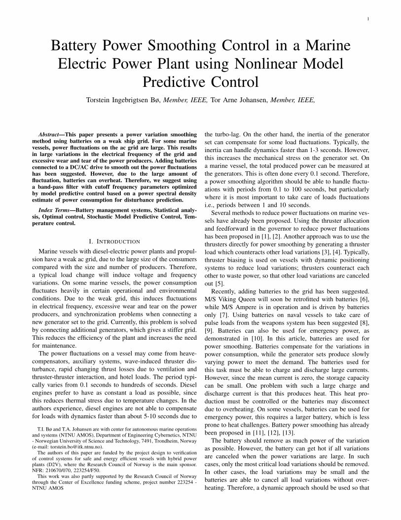
Fig. 1. Control hierarchy for power smoothing control. The thick linesrepresent electric power, while the thin lines represent control signals andmeasurements.

II. CONTROL PLANT

The control architecture is shown in Fig. 1. A load consumesthe load Pload, which is random. A battery is used to smooththe fluctuations in the generated power. The goal is to keepthe temperature and state of charge of the battery withinoperational limits, while reducing the power fluctuations inthe generator set as much as possible.

The charging and discharging power of the battery is givenby a band-pass filter. The input to the band-pass filter isPload, while the output is the desired charging power, Pref.This cancels out power fluctuations with frequencies betweenthe cut-off frequencies of the band-pass filter. This gives azero-mean charging power of the battery. However, the batterywill still be discharged even with zero-mean charging power,due to ohmic losses and self-discharge. To avoid the batterydischarging, the MPC calculates a mean charging power,PMPC.

It should be noted that the measurements of generated powermay not be synchronized and may have errors. In this study,we assume that the total consumed and generated power ismeasured without any error.

Heat generation due to high current through the battery mustbe limited to avoid it overheating. Therefore, the MPC adjuststhe time constants of the band-pass filter to avoid too highbattery temperatures.

A first-order high-pass filter and low-pass filter are put inseries to implement a band-pass filter. However, any linearband-pass filter could have been chosen. The transfer functionfor this filter is:

Hf (jω) =Pref(jω)

Pload(jω)=

τ jω

(1 +¯τjω)(1 + τ jω)ncells

(1)

where τ and¯τ are the highest and lowest time constants of

the band-pass filter, and ncells is the number of cells in thebattery. τ and

¯τ are set by the MPC controller.

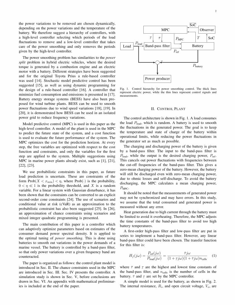
A simple model is used for the battery, as shown in Fig. 2.The internal resistance, Ri, and open circuit voltage, Vo, are

3

+− Vo

RiI

−

+

V

Fig. 2. Model of battery used internally in the MPC with internal resistance,Ri, and open circuit voltage, Vo, output voltage and current, V and I .

assumed to be constant. The temperature of the battery ismodeled by Newton’s law of cooling:

dTdt

=hA

c(Tair − T ) +

1

cQel (2)

where T is the battery temperature, h is the heat transfercoefficient, A is the surface area of the battery, c is the heatcapacity of the battery, Tair is the temperature of the coolingair, and Qel is the heat generated in the battery. The heat isassumed to be equal to the electrical loss

Qel = RiI2 (3)

where Ri is the internal resistance of the battery, and I is thecurrent through the battery.

Due to safety requirements the battery has a temperaturelimit for operation:

T ≤ Tmax. (4)

When this limit is reached, the battery must be disconnecteduntil it has cooled down.

The charging power, Pbattery, is controlled by a bi-directionalAC/DC converter. It is set to the sum of the references from theband-pass filter and the mean charging power, PMPC, calculatedby the MPC:

Pbattery = Pref + PMPC. (5)

Setting Pbattery = I(Vo + RiI), solving for the current, andusing the Taylor expansion we get:

I =−Vo +

√V 2o + 4RiPbattery

2Ri

=Pbattery

Vo−P 2

batteryRi

V 3o

+O(P 3battery) (6)

where O(P 3battery) denotes terms of order three or higher. The

first- and second-order approximations will be used later, thehigher order terms are assumed to be small.

The state of charge (SoC) of the battery is modeled as anintegrator of the current [15]:

dSoCdt

=I

Qnominal(7)

where Qnominal is the rated charge of the battery. Hence, theSoC of the battery is 0 when empty and 1 when fully charged.It is assumed that SoC is estimated by an external observer, asSoC estimates from Coulomb counting may drift-off. Multiplemethods exist for such estimations, e.g., [27], [28], [29].

The battery may also be used for emergency power. Wetherefore assume a minimum state of charge constraint:

SoCmin ≤ SoC ≤ SoCmax. (8)

The minimum and maximum state of charge can be set by anoperator or a plant optimizer. SoCmin and SoCmax can be usedto avoid the ageing of the lithium batteries as this acceleratesat low and high SoC.

However, since PLoad is stochastic we reformulate (8) totwo probabilistic constraints:

Prob(SoCmin ≤ SoC) ≥ 1− ηSoC

Prob(SoC ≤ SoCmax) ≥ 1− ηSoC(9)

where ηSoC is the chosen probability threshold for violation ofthe constraint.

The temperature of the battery depends on Pbattery. SincePbattery is random, T is also random. However, an estimate ofthe expected temperature is useful for the MPC. From (2):

ddtE[T ] =

hA

c(Tair − E[T ]) +

1

cE[Qel] (10)

using the linear approximation of the current from (6) (neglect-ing second-order and higher terms), the expected heat loss is:

E [Qel] ≈ E

[P 2

batteryRi

V 2o

](11)

Note that E[P 2

battery

]= P 2

MPC + σ2pref

, as E[Pref] = 0 due tothe band-pass filter and var [PMPC] = 0 (for one sample), thisgives E[PMPCPref] = 0 and

E [Qel] ≈ Ri

P 2MPC + σ2

pref

V 2o

. (12)

The variance of Pref can be estimated by (26) and (27)

σ2pref

=

∞∫0

ppp(ω)|Hf (jω)|2 dω. (13)

where ppp(ω) is the power spectral density of Pload.Note that the temperature variance will be small if the time

constant of the temperature (c/hA) is large compared withthe largest period in ppp(ω)|Hf (jω)|2 with significant power.Constraining the expected value is therefore reasonable. Alsonote that E[Qel(t)] is not constant due to the dependency ofthe states of the linear filter. However, we assume that the filtertime-constants are small compared with the time steps of theMPC. The temperature will therefore be close to the expectedvalue estimated above.

III. CHANCE CONSTRAINT

An example of how to approximate chance constraintsis given in this section. We need to convert the chanceconstraints (9) to explicit constraints. Assuming that Pload isclose to a normal distribution and the nonlinearities of theSoC dynamics are small, SoC can be approximated to benormal distributed. Using (28), the chance constraints can beapproximated to

SoCmin ≤ E[SoC]− F−1(1− ηSoC)σSoC

SoCmax ≥ E[SoC] + F−1(1− ηSoC)σSoC(14)

4

where F−1(·) is the inverse cumulative distribution functionof the standard normal distribution.

An estimate of E[SoC] and σ2SoC is needed. By using the ex-

pected value of (7) and using the second-order approximationof (6):

ddtE [SoC] ≈ E

[Pbattery

VoQnominal−

P 2batteryRi

V 3o Qnominal

]

=PMPC

VoQnominal−

(P 2MPC + σ2

pref)Ri

V 3o Qnominal

. (15)

By linearizing (6), a linear system from Pload to SoC isfound:

SoC(jω)

Pload(jω)=

Hf (jω)

QnominalVo(16)

The variance of SoC can be estimated by (16), (26) and (27)

σ2SoC ≈

∞∫0

ppp(ω)|Hf (jω)|2

Q2nominalV

2o

dω (17)

The state of charge can be approximated as a slowly varyingmean, E[SoC], with a superimposed noise, v.

SoC = E[SoC] + v (18)

where E[SoC] is calculated by (15). To estimate E[SoC] adiscrete Kalman filter is applied, where SoC is the “measuredstate”. The process is modeled as:

dSoCdt

=PMPC

VoQnominal−

(P 2MPC + σ2

pref)Ri

V 3o Qnominal

+ w (19)

y = SoC + v (20)

where SoC is the mean state of charge, E[SoC]; w is the“process noise”, which should capture the model errors ofE[SoC] including linearization errors and self-discharge; andv is the “measurement noise”, which is the current deviationof the state of charge from the mean state of charge. The noisev is approximated to be white noise with variance σ2

SoC. Thevariance of w is a tuning parameter for the filter. More detailson Kalman filters can be found in e.g., [30, ch. 5]. Note that asthe SoC cannot be directly measured it must be estimated. Inaddition, the terms “process noise” and “measurement noise”are misused to link the variables to commonly used terms forKalman filters (e.g., the variance of v is the variance of asignal, not the variance of a measurement error).

Both E[SoC] or σSoC can be controlled to fulfill (14).During the simulation study it was observed that when bothwere controlled the optimal solution was to reduce σSoCby decreasing the distance between

¯τ and τ . However, the

desired performance is that¯τ and τ are used to control

the temperature, while PMPC is used to control the SoC.Therefore, σSoC is set to max[σSoC(

¯τ, τ)] = σSoC(

¯τref, τref).

This gives a conservative performance of the SoC, and as longas SoCmax−SoCmin 2F−1(1−ηSoC)σSoC(

¯τref, τref) a feasible

E[SoC] exists.

IV. MODEL PREDICTIVE CONTROL

To achieve the control objectives mentioned in Sec. II, anMPC is implemented. The decision variables of the controllerare ξ =

[τ τ PMPC

]>, with reference values ξref. Some

slack variables are also used, to make sure that a feasiblesolution always exists, s =

[s+

SoC s−SoC sT]>

, with thereference sref. s+

SoC and s−SoC are slack variables for lower andupper SoC constraints, and sT is the slack variable for thetemperature constraint. The stage cost is:

l(ξ, s) =h1

(¯τ

¯τref− 1

)2

+ h2

( τref

τ− 1)2

+ h3P2MPC

+ (s− sref)>H2(s− sref) (21)

where h1, h2, and h3 are positive constants and H2 is apositive definite weight matrix. The chosen penalty functionof

¯τ and τ gives equal cost for doubling

¯τ as halving τ from

their reference. The costs of altering PMPC,¯τ , and τ are used

as tuning parameters as these are the control inputs to thebattery control system. This multi-objective cost function isequivalent to utopia tracking [31], with the exception of theneglected terminal constraint. Instead of terminal constraints,a long prediction horizon is used [32]. Other cost functions ofthe time constants were tested, such as:

l2 = (τ − τref)2 + (

¯τ −

¯τref)

2 (22)

l3 =

(1

τ− 1

τref

)2

+

(1

¯τ− 1

¯τref

)2

(23)

l4 = ln2

(τ

τref

)+ ln2

(¯τ

¯τref

)(24)

The l2 and l3 cost gives problems with scaling, as the MPCfavors adjusting one of the variables,

¯τ and τ , respectively.

Using a logarithmic cost, l4, gives solutions quite close tothose from using the chosen cost function. However, thiscost suffers from numerical problems and ACADO was oftenunable to solve the optimization problem.

The optimization problem is:

Ψ∗ = argminΨ

N−1∑k=0

l(ξ(tk), s(tk))

subject to (10), (15),

SoCmin ≤ E[SoC(tk)]− F−1(1− ηSoC)σSoC(tk) + s−SoC(tk)

SoCmax ≥ E[SoC(tk)] + F−1(1− ηSoC)σSoC(tk)− s+SoC(tk)

E[T (tk)] ≤ Tmax + sT (tk)

0 ≤ s(tk)

E[T (t0)] = T (t0)

E[SoC(t0)] = SoC(t0)(25)

where

Ψ =[ξ(t0) s(t0) . . . ξ(tN−1) s(tN−1)

]>contains all the decision variables and Ψ∗ is the optimalsolution. Note that all state constraints are soft, by the useof slack variables. This means that the optimization problemis always feasible.

5

+− Vo(T, SoC)

R0(T, SoC)

R1(T, SoC)

C1(T, SoC)

I

−

+

VT

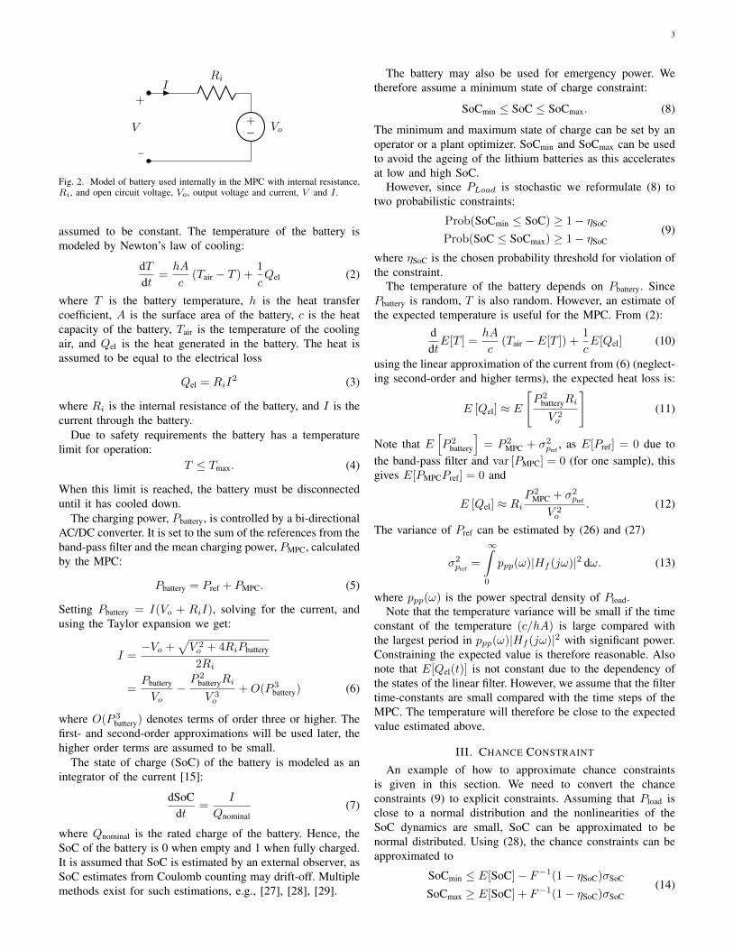
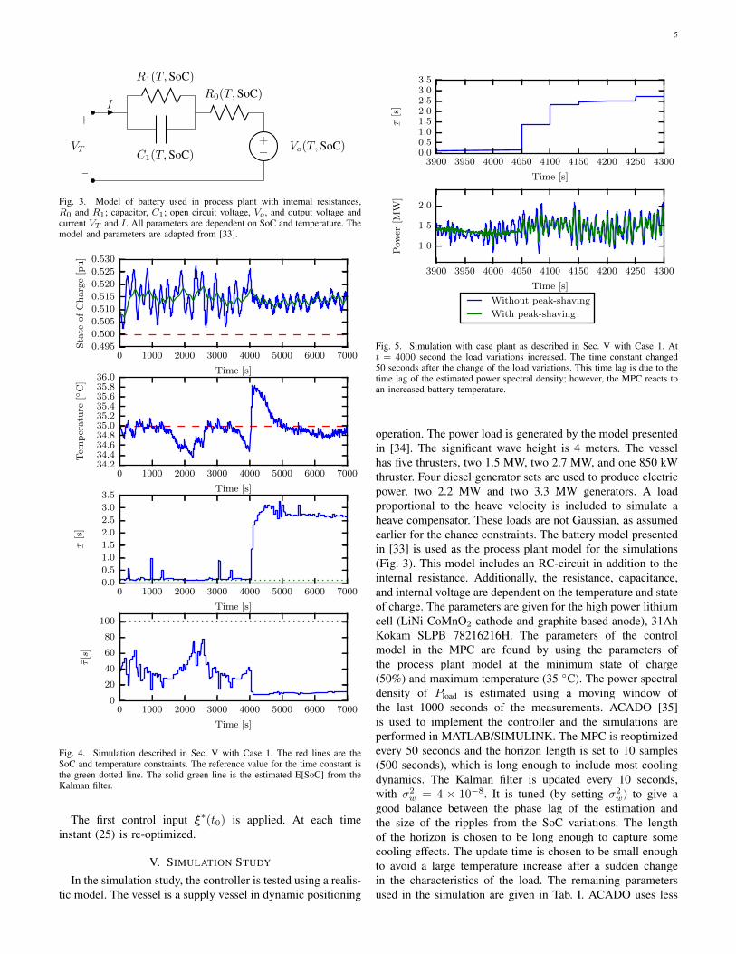
Fig. 3. Model of battery used in process plant with internal resistances,R0 and R1; capacitor, C1; open circuit voltage, Vo, and output voltage andcurrent VT and I . All parameters are dependent on SoC and temperature. Themodel and parameters are adapted from [33].

0 1000 2000 3000 4000 5000 6000 7000

Time [s]

0.495

0.500

0.505

0.510

0.515

0.520

0.525

0.530

Sta

teof

Ch

arg

e[p

u]

0 1000 2000 3000 4000 5000 6000 7000

Time [s]

34.234.434.634.835.035.235.435.635.836.0

Tem

per

atu

re[

C]

0 1000 2000 3000 4000 5000 6000 7000

Time [s]

0.0

0.5

1.0

1.5

2.0

2.5

3.0

3.5

¯τ[s

]

0 1000 2000 3000 4000 5000 6000 7000

Time [s]

0

20

40

60

80

100

τ[s

]

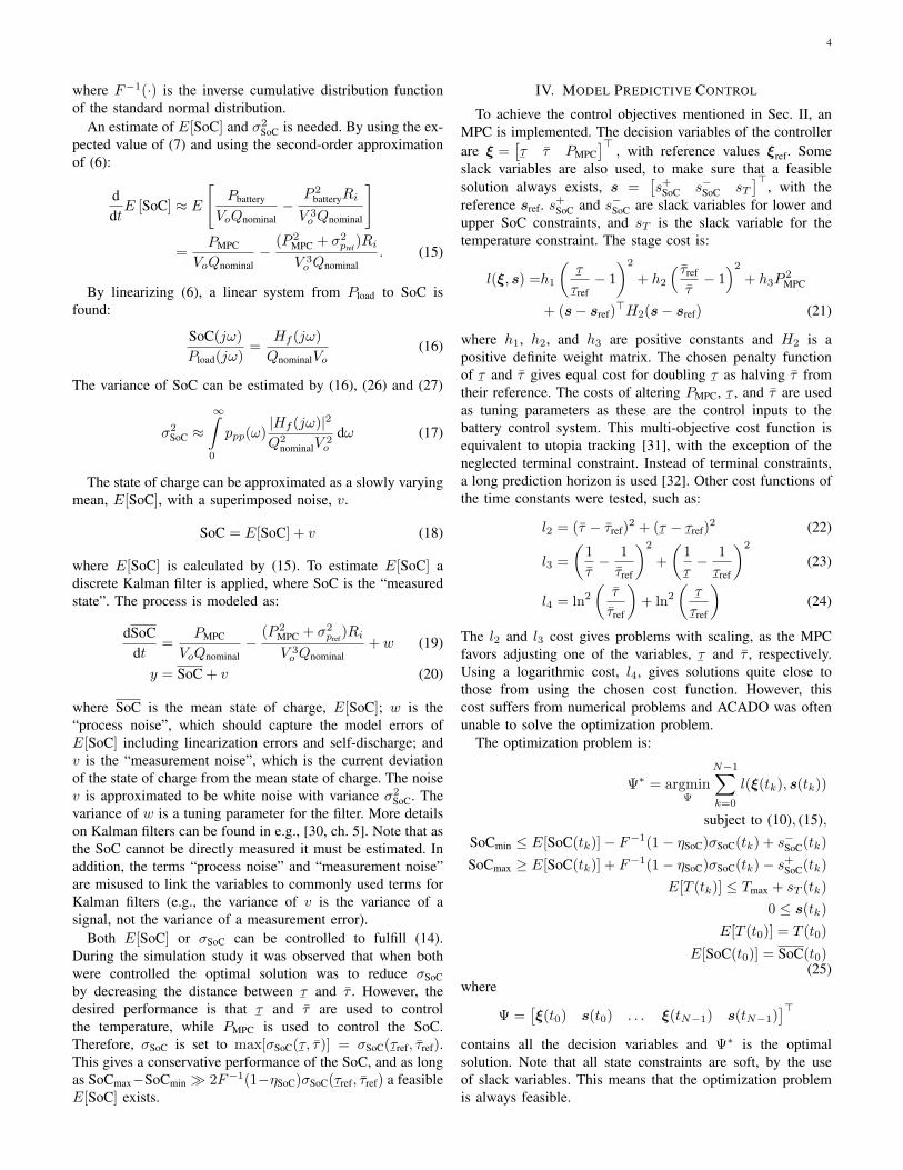
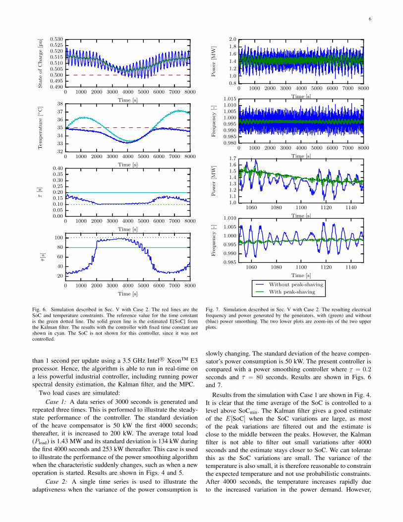
Fig. 4. Simulation described in Sec. V with Case 1. The red lines are theSoC and temperature constraints. The reference value for the time constant isthe green dotted line. The solid green line is the estimated E[SoC] from theKalman filter.

The first control input ξ∗(t0) is applied. At each timeinstant (25) is re-optimized.

V. SIMULATION STUDY

In the simulation study, the controller is tested using a realis-tic model. The vessel is a supply vessel in dynamic positioning

3900 3950 4000 4050 4100 4150 4200 4250 4300

Time [s]

0.00.51.01.52.02.53.03.5

¯τ[s

]

3900 3950 4000 4050 4100 4150 4200 4250 4300

Time [s]

1.0

1.5

2.0

Pow

er[M

W]

Without peak-shaving

With peak-shaving

Fig. 5. Simulation with case plant as described in Sec. V with Case 1. Att = 4000 second the load variations increased. The time constant changed50 seconds after the change of the load variations. This time lag is due to thetime lag of the estimated power spectral density; however, the MPC reacts toan increased battery temperature.

operation. The power load is generated by the model presentedin [34]. The significant wave height is 4 meters. The vesselhas five thrusters, two 1.5 MW, two 2.7 MW, and one 850 kWthruster. Four diesel generator sets are used to produce electricpower, two 2.2 MW and two 3.3 MW generators. A loadproportional to the heave velocity is included to simulate aheave compensator. These loads are not Gaussian, as assumedearlier for the chance constraints. The battery model presentedin [33] is used as the process plant model for the simulations(Fig. 3). This model includes an RC-circuit in addition to theinternal resistance. Additionally, the resistance, capacitance,and internal voltage are dependent on the temperature and stateof charge. The parameters are given for the high power lithiumcell (LiNi-CoMnO2 cathode and graphite-based anode), 31AhKokam SLPB 78216216H. The parameters of the controlmodel in the MPC are found by using the parameters ofthe process plant model at the minimum state of charge(50%) and maximum temperature (35 C). The power spectraldensity of Pload is estimated using a moving window ofthe last 1000 seconds of the measurements. ACADO [35]is used to implement the controller and the simulations areperformed in MATLAB/SIMULINK. The MPC is reoptimizedevery 50 seconds and the horizon length is set to 10 samples(500 seconds), which is long enough to include most coolingdynamics. The Kalman filter is updated every 10 seconds,with σ2

w = 4 × 10−8. It is tuned (by setting σ2w) to give a

good balance between the phase lag of the estimation andthe size of the ripples from the SoC variations. The lengthof the horizon is chosen to be long enough to capture somecooling effects. The update time is chosen to be small enoughto avoid a large temperature increase after a sudden changein the characteristics of the load. The remaining parametersused in the simulation are given in Tab. I. ACADO uses less

6

0 1000 2000 3000 4000 5000 6000 7000 8000

Time [s]

0.4900.4950.5000.5050.5100.5150.5200.5250.530

Sta

teof

Ch

arg

e[p

u]

0 1000 2000 3000 4000 5000 6000 7000 8000

Time [s]

32

33

34

35

36

37

38

Tem

per

atu

re[

C]

0 1000 2000 3000 4000 5000 6000 7000 8000

Time [s]

0.000.050.100.150.200.250.300.350.40

¯τ[s

]

0 1000 2000 3000 4000 5000 6000 7000 8000

Time [s]

20

40

60

80

100

τ[s

]

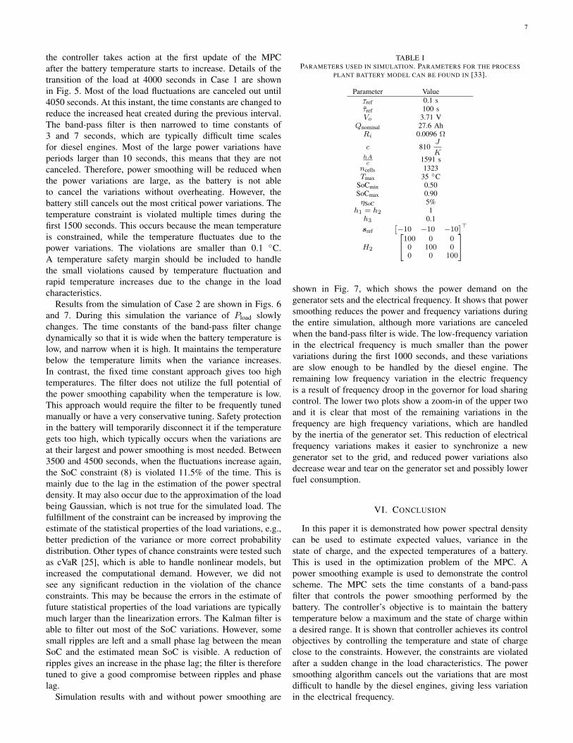
Fig. 6. Simulation described in Sec. V with Case 2. The red lines are theSoC and temperature constraints. The reference value for the time constantis the green dotted line. The solid green line is the estimated E[SoC] fromthe Kalman filter. The results with the controller with fixed time constant areshown in cyan. The SoC is not shown for this controller, since it was notcontrolled.

than 1 second per update using a 3.5 GHz Intel R© XeonTM E3processor. Hence, the algorithm is able to run in real-time ona less powerful industrial controller, including running powerspectral density estimation, the Kalman filter, and the MPC.

Two load cases are simulated:Case 1: A data series of 3000 seconds is generated and

repeated three times. This is performed to illustrate the steady-state performance of the controller. The standard deviationof the heave compensator is 50 kW the first 4000 seconds;thereafter, it is increased to 200 kW. The average total load(Pload) is 1.43 MW and its standard deviation is 134 kW duringthe first 4000 seconds and 253 kW thereafter. This case is usedto illustrate the performance of the power smoothing algorithmwhen the characteristic suddenly changes, such as when a newoperation is started. Results are shown in Figs. 4 and 5.

Case 2: A single time series is used to illustrate theadaptiveness when the variance of the power consumption is

0 1000 2000 3000 4000 5000 6000 7000 8000

Time [s]

0.8

1.0

1.2

1.4

1.6

1.8

2.0

Pow

er[M

W]

0 1000 2000 3000 4000 5000 6000 7000 8000

Time [s]

0.9800.9850.9900.9951.0001.0051.0101.015

Fre

qu

ency

[-]

1060 1080 1100 1120 1140

Time [s]

1.01.11.21.31.41.51.61.7

Pow

er[M

W]

1060 1080 1100 1120 1140

Time [s]

0.985

0.990

0.995

1.000

1.005

1.010F

requ

ency

[-]

Without peak-shaving

With peak-shaving

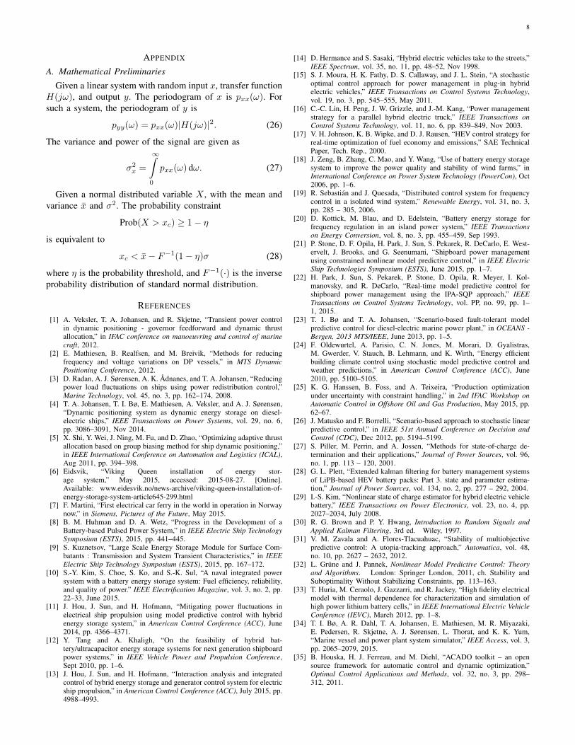
Fig. 7. Simulation described in Sec. V with Case 2. The resulting electricalfrequency and power generated by the generators, with (green) and without(blue) power smoothing. The two lower plots are zoom-ins of the two upperplots.

slowly changing. The standard deviation of the heave compen-sator’s power consumption is 50 kW. The present controller iscompared with a power smoothing controller where

¯τ = 0.2

seconds and τ = 80 seconds. Results are shown in Figs. 6and 7.

Results from the simulation with Case 1 are shown in Fig. 4.It is clear that the time average of the SoC is controlled to alevel above SoCmin. The Kalman filter gives a good estimateof the E[SoC] when the SoC variations are large, as mostof the peak variations are filtered out and the estimate isclose to the middle between the peaks. However, the Kalmanfilter is not able to filter out small variations after 4000seconds and the estimate stays closer to SoC. We can toleratethis as the SoC variations are small. The variance of thetemperature is also small, it is therefore reasonable to constrainthe expected temperature and not use probabilistic constraints.After 4000 seconds, the temperature increases rapidly dueto the increased variation in the power demand. However,

7

the controller takes action at the first update of the MPCafter the battery temperature starts to increase. Details of thetransition of the load at 4000 seconds in Case 1 are shownin Fig. 5. Most of the load fluctuations are canceled out until4050 seconds. At this instant, the time constants are changed toreduce the increased heat created during the previous interval.The band-pass filter is then narrowed to time constants of3 and 7 seconds, which are typically difficult time scalesfor diesel engines. Most of the large power variations haveperiods larger than 10 seconds, this means that they are notcanceled. Therefore, power smoothing will be reduced whenthe power variations are large, as the battery is not ableto cancel the variations without overheating. However, thebattery still cancels out the most critical power variations. Thetemperature constraint is violated multiple times during thefirst 1500 seconds. This occurs because the mean temperatureis constrained, while the temperature fluctuates due to thepower variations. The violations are smaller than 0.1 C.A temperature safety margin should be included to handlethe small violations caused by temperature fluctuation andrapid temperature increases due to the change in the loadcharacteristics.

Results from the simulation of Case 2 are shown in Figs. 6and 7. During this simulation the variance of Pload slowlychanges. The time constants of the band-pass filter changedynamically so that it is wide when the battery temperature islow, and narrow when it is high. It maintains the temperaturebelow the temperature limits when the variance increases.In contrast, the fixed time constant approach gives too hightemperatures. The filter does not utilize the full potential ofthe power smoothing capability when the temperature is low.This approach would require the filter to be frequently tunedmanually or have a very conservative tuning. Safety protectionin the battery will temporarily disconnect it if the temperaturegets too high, which typically occurs when the variations areat their largest and power smoothing is most needed. Between3500 and 4500 seconds, when the fluctuations increase again,the SoC constraint (8) is violated 11.5% of the time. This ismainly due to the lag in the estimation of the power spectraldensity. It may also occur due to the approximation of the loadbeing Gaussian, which is not true for the simulated load. Thefulfillment of the constraint can be increased by improving theestimate of the statistical properties of the load variations, e.g.,better prediction of the variance or more correct probabilitydistribution. Other types of chance constraints were tested suchas cVaR [25], which is able to handle nonlinear models, butincreased the computational demand. However, we did notsee any significant reduction in the violation of the chanceconstraints. This may be because the errors in the estimate offuture statistical properties of the load variations are typicallymuch larger than the linearization errors. The Kalman filter isable to filter out most of the SoC variations. However, somesmall ripples are left and a small phase lag between the meanSoC and the estimated mean SoC is visible. A reduction ofripples gives an increase in the phase lag; the filter is thereforetuned to give a good compromise between ripples and phaselag.

Simulation results with and without power smoothing are

TABLE IPARAMETERS USED IN SIMULATION. PARAMETERS FOR THE PROCESS

PLANT BATTERY MODEL CAN BE FOUND IN [33].

Parameter Value

¯τref 0.1 sτref 100 sVo 3.71 V

Qnominal 27.6 AhRi 0.0096 Ω

c 810J

KhAc

1591 sncells 1323Tmax 35 C

SoCmin 0.50SoCmax 0.90ηSoC 5%

h1 = h2 1h3 0.1sref

[−10 −10 −10

]>H2

100 0 00 100 00 0 100

shown in Fig. 7, which shows the power demand on thegenerator sets and the electrical frequency. It shows that powersmoothing reduces the power and frequency variations duringthe entire simulation, although more variations are canceledwhen the band-pass filter is wide. The low-frequency variationin the electrical frequency is much smaller than the powervariations during the first 1000 seconds, and these variationsare slow enough to be handled by the diesel engine. Theremaining low frequency variation in the electric frequencyis a result of frequency droop in the governor for load sharingcontrol. The lower two plots show a zoom-in of the upper twoand it is clear that most of the remaining variations in thefrequency are high frequency variations, which are handledby the inertia of the generator set. This reduction of electricalfrequency variations makes it easier to synchronize a newgenerator set to the grid, and reduced power variations alsodecrease wear and tear on the generator set and possibly lowerfuel consumption.

VI. CONCLUSION

In this paper it is demonstrated how power spectral densitycan be used to estimate expected values, variance in thestate of charge, and the expected temperatures of a battery.This is used in the optimization problem of the MPC. Apower smoothing example is used to demonstrate the controlscheme. The MPC sets the time constants of a band-passfilter that controls the power smoothing performed by thebattery. The controller’s objective is to maintain the batterytemperature below a maximum and the state of charge withina desired range. It is shown that controller achieves its controlobjectives by controlling the temperature and state of chargeclose to the constraints. However, the constraints are violatedafter a sudden change in the load characteristics. The powersmoothing algorithm cancels out the variations that are mostdifficult to handle by the diesel engines, giving less variationin the electrical frequency.

8

APPENDIX

A. Mathematical Preliminaries

Given a linear system with random input x, transfer functionH(jω), and output y. The periodogram of x is pxx(ω). Forsuch a system, the periodogram of y is

pyy(ω) = pxx(ω)|H(jω)|2. (26)

The variance and power of the signal are given as

σ2x =

∞∫0

pxx(ω) dω. (27)

Given a normal distributed variable X , with the mean andvariance x and σ2. The probability constraint

Prob(X > xc) ≥ 1− η

is equivalent to

xc < x− F−1(1− η)σ (28)

where η is the probability threshold, and F−1(·) is the inverseprobability distribution of standard normal distribution.

REFERENCES

[1] A. Veksler, T. A. Johansen, and R. Skjetne, “Transient power controlin dynamic positioning - governor feedforward and dynamic thrustallocation,” in IFAC conference on manoeuvring and control of marinecraft, 2012.

[2] E. Mathiesen, B. Realfsen, and M. Breivik, “Methods for reducingfrequency and voltage variations on DP vessels,” in MTS DynamicPositioning Conference, 2012.

[3] D. Radan, A. J. Sørensen, A. K. Adnanes, and T. A. Johansen, “Reducingpower load fluctuations on ships using power redistribution control,”Marine Technology, vol. 45, no. 3, pp. 162–174, 2008.

[4] T. A. Johansen, T. I. Bø, E. Mathiesen, A. Veksler, and A. J. Sørensen,“Dynamic positioning system as dynamic energy storage on diesel-electric ships,” IEEE Transactions on Power Systems, vol. 29, no. 6,pp. 3086–3091, Nov 2014.

[5] X. Shi, Y. Wei, J. Ning, M. Fu, and D. Zhao, “Optimizing adaptive thrustallocation based on group biasing method for ship dynamic positioning,”in IEEE International Conference on Automation and Logistics (ICAL),Aug 2011, pp. 394–398.

[6] Eidsvik, “Viking Queen installation of energy stor-age system,” May 2015, accessed: 2015-08-27. [Online].Available: www.eidesvik.no/news-archive/viking-queen-installation-of-energy-storage-system-article645-299.html

[7] F. Martini, “First electrical car ferry in the world in operation in Norwaynow,” in Siemens, Pictures of the Future, May 2015.

[8] B. M. Huhman and D. A. Wetz, “Progress in the Development of aBattery-based Pulsed Power System,” in IEEE Electric Ship TechnologySymposium (ESTS), 2015, pp. 441–445.

[9] S. Kuznetsov, “Large Scale Energy Storage Module for Surface Com-batants : Transmission and System Transient Characteristics,” in IEEEElectric Ship Technology Symposium (ESTS), 2015, pp. 167–172.

[10] S.-Y. Kim, S. Choe, S. Ko, and S.-K. Sul, “A naval integrated powersystem with a battery energy storage system: Fuel efficiency, reliability,and quality of power.” IEEE Electrification Magazine, vol. 3, no. 2, pp.22–33, June 2015.

[11] J. Hou, J. Sun, and H. Hofmann, “Mitigating power fluctuations inelectrical ship propulsion using model predictive control with hybridenergy storage system,” in American Control Conference (ACC), June2014, pp. 4366–4371.

[12] Y. Tang and A. Khaligh, “On the feasibility of hybrid bat-tery/ultracapacitor energy storage systems for next generation shipboardpower systems,” in IEEE Vehicle Power and Propulsion Conference,Sept 2010, pp. 1–6.

[13] J. Hou, J. Sun, and H. Hofmann, “Interaction analysis and integratedcontrol of hybrid energy storage and generator control system for electricship propulsion,” in American Control Conference (ACC), July 2015, pp.4988–4993.

[14] D. Hermance and S. Sasaki, “Hybrid electric vehicles take to the streets,”IEEE Spectrum, vol. 35, no. 11, pp. 48–52, Nov 1998.

[15] S. J. Moura, H. K. Fathy, D. S. Callaway, and J. L. Stein, “A stochasticoptimal control approach for power management in plug-in hybridelectric vehicles,” IEEE Transactions on Control Systems Technology,vol. 19, no. 3, pp. 545–555, May 2011.

[16] C.-C. Lin, H. Peng, J. W. Grizzle, and J.-M. Kang, “Power managementstrategy for a parallel hybrid electric truck,” IEEE Transactions onControl Systems Technology, vol. 11, no. 6, pp. 839–849, Nov 2003.

[17] V. H. Johnson, K. B. Wipke, and D. J. Rausen, “HEV control strategy forreal-time optimization of fuel economy and emissions,” SAE TechnicalPaper, Tech. Rep., 2000.

[18] J. Zeng, B. Zhang, C. Mao, and Y. Wang, “Use of battery energy storagesystem to improve the power quality and stability of wind farms,” inInternational Conference on Power System Technology (PowerCon), Oct2006, pp. 1–6.

[19] R. Sebastian and J. Quesada, “Distributed control system for frequencycontrol in a isolated wind system,” Renewable Energy, vol. 31, no. 3,pp. 285 – 305, 2006.

[20] D. Kottick, M. Blau, and D. Edelstein, “Battery energy storage forfrequency regulation in an island power system,” IEEE Transactionson Energy Conversion, vol. 8, no. 3, pp. 455–459, Sep 1993.

[21] P. Stone, D. F. Opila, H. Park, J. Sun, S. Pekarek, R. DeCarlo, E. West-ervelt, J. Brooks, and G. Seenumani, “Shipboard power managementusing constrained nonlinear model predictive control,” in IEEE ElectricShip Technologies Symposium (ESTS), June 2015, pp. 1–7.

[22] H. Park, J. Sun, S. Pekarek, P. Stone, D. Opila, R. Meyer, I. Kol-manovsky, and R. DeCarlo, “Real-time model predictive control forshipboard power management using the IPA-SQP approach,” IEEETransactions on Control Systems Technology, vol. PP, no. 99, pp. 1–1, 2015.

[23] T. I. Bø and T. A. Johansen, “Scenario-based fault-tolerant modelpredictive control for diesel-electric marine power plant,” in OCEANS -Bergen, 2013 MTS/IEEE, June 2013, pp. 1–5.

[24] F. Oldewurtel, A. Parisio, C. N. Jones, M. Morari, D. Gyalistras,M. Gwerder, V. Stauch, B. Lehmann, and K. Wirth, “Energy efficientbuilding climate control using stochastic model predictive control andweather predictions,” in American Control Conference (ACC), June2010, pp. 5100–5105.

[25] K. G. Hanssen, B. Foss, and A. Teixeira, “Production optimizationunder uncertainty with constraint handling,” in 2nd IFAC Workshop onAutomatic Control in Offshore Oil and Gas Production, May 2015, pp.62–67.

[26] J. Matusko and F. Borrelli, “Scenario-based approach to stochastic linearpredictive control,” in IEEE 51st Annual Conference on Decision andControl (CDC), Dec 2012, pp. 5194–5199.

[27] S. Piller, M. Perrin, and A. Jossen, “Methods for state-of-charge de-termination and their applications,” Journal of Power Sources, vol. 96,no. 1, pp. 113 – 120, 2001.

[28] G. L. Plett, “Extended kalman filtering for battery management systemsof LiPB-based HEV battery packs: Part 3. state and parameter estima-tion,” Journal of Power Sources, vol. 134, no. 2, pp. 277 – 292, 2004.

[29] I.-S. Kim, “Nonlinear state of charge estimator for hybrid electric vehiclebattery,” IEEE Transactions on Power Electronics, vol. 23, no. 4, pp.2027–2034, July 2008.

[30] R. G. Brown and P. Y. Hwang, Introduction to Random Signals andApplied Kalman Filtering, 3rd ed. Wiley, 1997.

[31] V. M. Zavala and A. Flores-Tlacuahuac, “Stability of multiobjectivepredictive control: A utopia-tracking approach,” Automatica, vol. 48,no. 10, pp. 2627 – 2632, 2012.

[32] L. Grune and J. Pannek, Nonlinear Model Predictive Control: Theoryand Algorithms. London: Springer London, 2011, ch. Stability andSuboptimality Without Stabilizing Constraints, pp. 113–163.

[33] T. Huria, M. Ceraolo, J. Gazzarri, and R. Jackey, “High fidelity electricalmodel with thermal dependence for characterization and simulation ofhigh power lithium battery cells,” in IEEE International Electric VehicleConference (IEVC), March 2012, pp. 1–8.

[34] T. I. Bø, A. R. Dahl, T. A. Johansen, E. Mathiesen, M. R. Miyazaki,E. Pedersen, R. Skjetne, A. J. Sørensen, L. Thorat, and K. K. Yum,“Marine vessel and power plant system simulator,” IEEE Access, vol. 3,pp. 2065–2079, 2015.

[35] B. Houska, H. J. Ferreau, and M. Diehl, “ACADO toolkit – an opensource framework for automatic control and dynamic optimization,”Optimal Control Applications and Methods, vol. 32, no. 3, pp. 298–312, 2011.