Batch Learning from Logged Bandit Feedback through ... Learning from Logged Bandit Feedback through Counterfactual Risk Minimization Adith Swaminathan [email protected] Department

Journal of Machine Learning Research 1 (2015) 1-25 Submitted 6/15; Published

Batch Learning from Logged Bandit Feedback throughCounterfactual Risk Minimization

Adith Swaminathan [email protected] of Computer ScienceCornell UniversityIthaca, NY 14853, USA

Thorsten Joachims [email protected]

Department of Computer Science

Cornell University

Ithaca, NY 14853, USA

Editor: Vladimir N.Vapnik, Alexander Gammerman, Vladimir Vovk

Abstract

We develop a learning principle and an efficient algorithm for batch learning from loggedbandit feedback. This learning setting is ubiquitous in online systems (e.g., ad placement,web search, recommendation), where an algorithm makes a prediction (e.g., ad ranking)for a given input (e.g., query) and observes bandit feedback (e.g., user clicks on presentedads). We first address the counterfactual nature of the learning problem (Bottou et al.,2013) through propensity scoring. Next, we prove generalization error bounds that ac-count for the variance of the propensity-weighted empirical risk estimator. In analogy tothe Structural Risk Minimization principle of Wapnik and Tscherwonenkis (1979), theseconstructive bounds give rise to the Counterfactual Risk Minimization (CRM) principle.We show how CRM can be used to derive a new learning method—called Policy Optimizerfor Exponential Models (POEM)—for learning stochastic linear rules for structured out-put prediction. We present a decomposition of the POEM objective that enables efficientstochastic gradient optimization. The effectiveness and efficiency of POEM is evaluatedon several simulated multi-label classification problems, as well as on a real-world informa-tion retrieval problem. The empirical results show that the CRM objective implementedin POEM provides improved robustness and generalization performance compared to thestate-of-the-art.

Keywords: empirical risk minimization, bandit feedback, importance sampling, propen-sity score matching, structured prediction

1. Introduction

Log data is one of the most ubiquitous forms of data available, as it can be recordedfrom a variety of systems (e.g., search engines, recommender systems, ad placement) atlittle cost. The interaction logs of such systems typically contain a record of the input tothe system (e.g., features describing the user), the prediction made by the system (e.g., arecommended list of news articles) and the feedback (e.g., number of ranked articles the userread) (Li et al., 2010). The feedback, however, provides only partial information— “banditfeedback”— limited to the particular prediction shown by the system. The feedback for

c©2015 Adith Swaminathan and Thorsten Joachims.

Swaminathan and Joachims

all the other predictions the system could have made is typically not known. This makeslearning from log data fundamentally different from supervised learning, where “correct”predictions (e.g., the best ranking of news articles for that user) together with a loss functionprovide full-information feedback.

In this paper, we address the problem of learning from logged bandit feedback. Unlikeonline learning with bandit feedback, batch learning with bandit feedback does not requireinteractive experimental control over the system. Furthermore, it enables the reuse ofexisting data and offline cross-validation techniques for model selection (e.g., “which featuresto use?”, “which learning algorithm to use?”, etc.).

To design algorithms for batch learning from bandit feedback, counterfactual estimators(Bottou et al., 2013) of a system’s performance can be used to estimate how other systemswould have performed if they had been in control of choosing predictions. Such estimatorshave been developed recently for the off-policy evaluation problem (Dudık et al., 2011; Liet al., 2011, 2014), where data collected from the interaction logs of one bandit algorithmis used to evaluate another system.

Our approach to counterfactual learning centers around the insight that, to perform ro-bust learning, it is not sufficient to have just an unbiased estimator of the off-policy system’sperformance. We must also reason about how the variances of these estimators differ acrossthe hypothesis space, and pick the hypothesis that has the best possible guarantee (tightestconservative bound) for its performance. We first prove generalization error bounds fora stochastic hypothesis family using an empirical Bernstein argument (Maurer and Pontil,2009). This builds on recent approaches to deriving confidence intervals for counterfactualestimators (Bottou et al., 2013; Thomas et al., 2015). By relating the generalization errorto the empirical sample variance of different hypotheses, we can effectively penalize the hy-potheses with large variance during training using a data-dependant regularizer. In analogyto Structural Risk Minimization for full-information feedback (Wapnik and Tscherwonenkis,1979), the constructive nature of these bounds suggests a general principle—CounterfactualRisk Minimization (CRM)—for designing methods for batch learning from bandit feedback.

Using the CRM principle, we derive a new learning algorithm—Policy Optimizer forExponential Models (POEM)—for structured output prediction. The training objective isdecomposed using repeated variance linearization, and optimizing it using AdaGrad (Duchiet al., 2011) yields a fast and effective algorithm. We evaluate POEM on several multi-label classification problems, verify that its empirical performance supports the theory, anddemonstrates substantial gain in generalization performance over the state-of-the-art.

This paper is an extended version of Swaminathan and Joachims (2015), adding thefollowing contributions. First, it provides the proof of the main generalization error boundupon which the CRM principle is based. Second, it derives and details the Iterated VarianceMajorization Algorithm for training POEM, which was only sketched in Swaminathan andJoachims (2015). Third, the paper provides a first real-world experiment using POEM forlearning a high precision classifier for information retrieval using logged click data.

The remainder of this paper is structured as follows. We review existing approachesin Section 2. The learning setting is detailed in Section 3, and contrasted with supervisedlearning. In Section 4, we derive the Counterfactual Risk Minimization learning principleand provide a rule of thumb for setting hyper-parameters. In Section 5, we instantiate theCRM principle for structured output prediction using exponential models and construct an

2

Counterfactual Risk Minimization

efficient decomposition of the objective for stochastic optimization. Empirical evaluationsare reported in Section 6 and a real-world application is described in Section 7. We concludewith future directions and discussion in Section 8.

2. Related Work

Existing approaches for batch learning from logged bandit feedback fall into two categories.The first approach is to reduce the problem to supervised learning. In principle, since thelogs give us an incomplete view of the feedback for different predictions, one could first useregression to estimate a feedback oracle for unseen predictions, and then use any supervisedlearning algorithm using this feedback oracle. Such a two-stage approach is known to notgeneralize well (Beygelzimer and Langford, 2009). More sophisticated techniques using theOffset Tree algorithm (Beygelzimer and Langford, 2009) allow us to perform batch learn-ing when the space of possible predictions is small. In contrast, our approach generalizesstructured output prediction, with exponential-sized prediction spaces. In particular, weapply our approach to multilabel classification problems. When the number of labels is K,the number of possible predictions is 2K . A direct application of the Offset tree algorithmrequires O(2K) space and only guarantees regret O((2K − 1)r) where r is the regret ofthe underlying binary classifier. Our approach directly tackles the problem using popularmodels from structured prediction instead, using computation and space complexity thatmimics supervised approaches to the problem.

The second approach to batch learning from bandit feedback uses propensity scoring(Rosenbaum and Rubin, 1983) to derive unbiased estimators from the interaction logs (Bot-tou et al., 2013). These estimators are used for a small set of candidate policies, and thebest estimated candidate is picked via exhaustive search. In contrast, our approach can beoptimized via gradient descent, over hypothesis families (of infinite size) that are equally asexpressive as those used in supervised learning. In particular, we build on recent work thatdevelops confidence bounds for counterfactual estimators (Bottou et al., 2013; Thomas et al.,2015) using empirical Bernstein bounds. Our key insight is that these confidence intervalsare not merely observable but can be efficiently optimized during training. Other recentbounds derived from analyzing Renyi divergences (Cortes et al., 2010) can analogously beco-opted in our approach to counterfactual learning.

Our approach builds on counterfactual estimators that have been developed for off-policy evaluation. The inverse propensity scoring approach can work well when we havea good model of the historical algorithm (Strehl et al., 2010; Li et al., 2014, 2015), anddoubly robust estimators (Dudık et al., 2011) are even more effective when we additionallyhave a good model of the feedback. In our work, we focus on the inverse propensity scoringestimator, but the results we derive hold equally for the doubly robust estimators.

In the current work, we concentrate on the case where the historical algorithm was astationary, stochastic policy. Techniques like exploration scavenging (Langford et al., 2008)and bootstrapping (Mary et al., 2014) allow us to perform counterfactual evaluation evenwhen the historical algorithm was deterministic or adaptive.

Our strategy of picking the hypothesis with the tightest conservative bound on per-formance mimics similar successful approaches in other problems like supervised learning(Wapnik and Tscherwonenkis, 1979), risk averse multi-armed bandits (Galichet et al., 2013),

3


regret minimizing contextual bandits (Langford and Zhang, 2008) and reinforcement learn-ing (Garcia and Fernandez, 2012). Beyond the problem of batch learning from banditfeedback, our approach can have implications for several applications that require learningfrom logged bandit feedback data: warm-starting multi-armed bandits (Shivaswamy andJoachims, 2012) and contextual bandits (Strehl et al., 2010), pre-selecting retrieval func-tions for search engines (Hofmann et al., 2013), policy evaluation for contextual bandits (Liet al., 2011), and reinforcement learning (Thomas et al., 2015) to name a few.

3. Learning Setting: Batch Learning with Logged Bandit Feedback

Consider a structured output prediction problem that takes as input x ∈ X and outputs aprediction y ∈ Y. For example, in multi-label document classification, x could be a newsarticle and y a bitvector indicating the labels assigned to this article. The inputs are assumed

drawn from a fixed but unknown distribution Pr(X ), xi.i.d.∼ Pr(X ). Consider a hypothesis

space H of stochastic policies. A hypothesis h(Y | x) ∈ H defines a probability distributionover the output space Y, and the hypothesis makes predictions by sampling, y ∼ h(Y | x).Note that this definition also includes deterministic hypotheses, where the distributionsassign probability 1 to a single y. For notational convenience, denote h(Y | x) by h(x), andthe probability assigned by h(x) to y as h(y | x). We will abuse notation slightly and use(x, y) ∼ h to refer to samples drawn from the joint distribution, x ∼ Pr(X ), y ∼ h(Y | x).When it is clear from the context, we will drop (x, y) ∼ h and simply write h.

In interactive learning systems, we only observe feedback δ(x, y) for the y sampled fromh(x). In this work, feedback δ : X × Y 7→ R is a cardinal loss that is only observed at thesampled data points. Small values for δ(x, y) indicate user satisfaction with y for x, whilelarge values indicate dissatisfaction. The expected loss—called risk—of a hypothesis R(h)is defined as,

R(h) = Ex∼Pr(X )Ey∼h(x) [δ(x, y)] = Eh [δ(x, y)] .

The goal of the system is to minimize risk, or equivalently, maximize expected user satis-faction. The aim of learning is to find a hypothesis h ∈ H that has minimum risk.

We wish to re-use the interaction logs of these systems for batch learning. Assume thatits historical algorithm acted according to a stationary policy h0(x) (also called loggingpolicy). The data collected from this system is

D = {(x1, y1, δ1), . . . , (xn, yn, δn)},

where yi ∼ h0(xi) and δi ≡ δ(xi, yi).Sampling bias. D cannot be used to estimate R(h) for a new hypothesis h using the

estimator typically used in supervised learning. We ideally need either full informationabout δ(xi, ·) or need samples y ∼ h(xi) to directly estimate R(h). This explains why, inpractice, model selection over a small set of candidate systems is typically done via A/Btests, where the candidates are deployed to collect new data sampled according to y ∼ h(x)for each hypothesis h. A relative comparison of the assumptions, hypotheses, and principlesused in supervised learning vs. our learning setting is outlined in Table 1. Fundamentally,batch learning with bandit feedback is hard because D is both biased (predictions favoredby the historical algorithm will be over-represented) and incomplete (feedback for otherpredictions will not be available) for learning.

4


Supervised Batch w/bandit

Distribution (x, y∗) ∼ Pr(X × Y) x ∼ Pr(X ), y ∼ h0(x)Data D {xi, y∗i } {xi, yi, δi, pi}Hypothesis h y = h(x) y ∼ h(Y | x)Loss ∆(y∗, ·) known δ(x, ·) unknown

Objective: argminh R(h) + C ·Reg(H) RM (h) + C ·Reg(H) + λ ·√

V ar(h)n

Table 1: Comparison of assumptions, hypotheses and learning principles for supervisedlearning and batch learning with bandit feedback.

4. Learning Principle: Counterfactual Risk Minimization

The distribution mismatch between h0 and any hypothesis h ∈ H can be addressed usingimportance sampling, which corrects the sampling bias as:

R(h) = Eh [δ(x, y)] = Eh0[δ(x, y)

h(y | x)

h0(y | x)

].

This motivates the propensity scoring approach of Rosenbaum and Rubin (1983). Duringthe operation of the logging policy, we keep track of the propensity, h0(y | x) of the historicalsystem to generate y for x. From these propensity-augmented logs

D = {(x1, y1, δ1, p1), . . . , (xn, yn, δn, pn)},

where pi ≡ h0(yi | xi), we can derive an unbiased estimate of R(h) via Monte Carloapproximation,

R(h) =1

n

n∑i=1

δih(yi | xi)

pi. (1)

At first thought, one may think that directly estimating R(h) over h ∈ H and picking theempirical minimizer is a valid learning strategy. Unfortunately, there are several pitfalls.

First, this strategy is not invariant to additive transformations of the loss and willgive degenerate results if the loss is not appropriately scaled. In Section 4.3, we developintuition for why this is so, and derive the optimal scaling of δ. For now, assume that∀x,∀y, δ(x, y) ∈ [−1, 0].

Second, this estimator has unbounded variance, since pi ' 0 in D can cause R(h) to bearbitrarily far away from the true risk R(h). This can be fixed by “clipping” the importancesampling weights (Ionides, 2008; Strehl et al., 2010; Bottou et al., 2013; Cortes et al., 2010)

RM (h) = Eh0[δ(x, y) min

{M,

h(y | x)

h0(y | x)

}],

RM (h) =1

n

n∑i=1

δi min

{M,

h(yi | xi)pi

}.

5


M ≥ 1 is a hyper-parameter chosen to trade-off bias and variance in the estimate, wheresmaller values of M induce larger bias in the estimate. Optimizing RM (h) through exhaus-tive enumeration over H yields the Inverse Propensity Scoring (IPS) training objective

hIPS = argminh∈H

{RM (h)

}. (2)

This objective captures the essence of previous offline policy optimization approaches (Bot-tou et al., 2013; Strehl et al., 2010). These approaches differ from Equation (2) in the specificway the importance sampling weights are clipped, and frame the optimization problem as amaximization of counterfactual rewards as opposed to minimization of counterfactual risk.

Third, importance sampling typically estimates RM (h) of different hypotheses h ∈ Hwith vastly different variances. Consider two hypotheses h1 and h2, where h1 is similar toh0, but where h2 samples predictions that were not well explored by h0. Importance sam-pling gives us low-variance estimates for RM (h1), but highly variable estimates for RM (h2).Intuitively, if we can develop variance-sensitive confidence bounds over the hypothesis space,optimizing a conservative confidence bound should find a h whose R(h) will not be muchworse, with high probability.

4.1 Generalization Error Bound

A standard analysis would give a bound that is agnostic to the variance introduced byimportance sampling. Following our intuition above, we derive a higher order bound thatincludes the variance term using empirical Bernstein bounds (Maurer and Pontil, 2009). Todevelop such a generalization error bound, we first need a concept of capacity for stochastichypothesis classes. Our strategy is to define an auxiliary deterministic function class FHfor H and directly use covering numbers for FH conditioned on a sample D. We start bydefining the auxiliary deterministic function class FH.

Definition 1 For any stochastic class H, define an auxiliary function class FH = {fh :X × Y 7→ [0, 1]}. Each h ∈ H corresponds to a function fh ∈ FH,

fh(x, y) = 1 +δ(x, y)

Mmin

{M,

h(y | x)

h0(y | x)

}. (3)

Based on this auxiliarity function class FH, we will study the convergence of RM (h)→RM (h). A key insight is the following relationship between h and fh.

Lemma 2 For any stochastic hypothesis h, the clipped risk RM (h) and the expected valueof fh under the data generating distribution are related as

Eh0 [fh(x, y)] = 1 +RM (h)

M. (4)

6


Proof Note that fh is a deterministic and bounded function. From the definition of fhand by linearity of expectation,

Eh0 [fh(x, y)] = Eh0[1 +

δ(x, y)

Mmin

{M,

h(y | x)

h0(y | x)

}]= 1 +

1

MEh0

[δ(x, y) min

{M,

h(y | x)

h0(y | x)

}]= 1 +

RM (h)

M

As a consequence of Lemma 2, we can use classic notions of capacity for FH to reasonabout the convergence of RM (h) → RM (h). Recall the covering number N∞(ε,F , n) for afunction class F .1 Define an ε−cover N (ε, A, ‖ · ‖∞) for a set A ⊆ Rn to be the size of thesmallest cardinality subset A0 ⊆ A such that A is contained in the union of balls of radiusε centered at points in A0, in the metric induced by ‖ · ‖∞. The covering number is,

N∞(ε,F , n) = sup(xi,yi)∈(X×Y)n

N (ε,F({(xi, yi)}), ‖ · ‖∞),

where F({(xi, yi)}) is the function class conditioned on sample {(xi, yi)},

F({(xi, yi)}) = {(f(x1, y1), . . . , f(xn, yn)) : f ∈ F}.

Our measure for the capacity of our stochastic class H to “fit” a sample of size n shall beN∞( 1

n ,FH, 2n).

For a compact notation, define the random variable uh ≡ δ(x, y) min{M, h(y|x)h0(y|x)

}with

mean uh = RM (h). The sampleD contains n i.i.d. random variables uhi ≡ δi min{M, h(yi|xi)pi

}.Define the sample mean and variance of uh

i

uh ≡1

n

n∑i=1

uhi = RM (h),

ˆV ar(uh) ≡ 1

n− 1

n∑i=1

(uhi − uh)2.

Theorem 3 With probability at least 1−γ in the random vector (x1, y1) · · · (xn, yn)i.i.d.∼ h0,

with observed losses δ1, . . . , δn, for n ≥ 16 and a stochastic hypothesis space H with capacityN∞( 1

n ,FH, 2n),

∀h ∈ H : R(h) ≤ RM (h) +

√18

ˆV ar(uh)QH(n, γ)

n+M

15QH(n, γ)

n− 1,

where, QH(n, γ) ≡ log(10 · N∞( 1

n ,FH, 2n)

γ), 0 < γ < 1.

1. Refer Anthony and Bartlett (2009); Maurer and Pontil (2009) and the references therein for a compre-hensive treatment of covering numbers.

7


Proof The proof follows from Theorem 6 of Maurer and Pontil (2009) applied to thedeterministic function class FH. We sketch the main argument using symmetrization andRademacher variables here.

Define the random variable sh = 1 + uhM with mean Eh0 [sh] and variance V ar(sh).

Observe that Eh0 [sh] = 1 + RM (h)M from Lemma 2. Let sh

i = 1 + uhi

M . The sample Dessentially contains n i.i.d. observations of sh. Let sh and ˆV ar(sh) denote the empirical

mean and variance of {shi}ni=1 respectively. Observe that ˆV ar(sh) =ˆV ar(uh)M2 . Abusing

notation slightly, we will use boldface sh to refer to the sample {shi}ni=1.We begin with Bennet’s inequality.For s, {si}ni=1 i.i.d. bounded random variables in [0, 1] having mean E [s] and variance

V ar(s), with probability at least 1− γ in {si}ni=1 ≡ s,

E [s]− s ≤√

2V ar(s) log 1/γ

n+

log 1/γ

3n. (5)

Intuitively, Bennet’s inequality tells us that the estimate s has lower accuracy if V ar(s)is high, which exactly captures our intuition about the variance introduced by importancesampling when estimating the risk of a hypothesis “far” from h0. However, the diameter ofthis confidence interval depends on the unobservable V ar(s).

We recite Theorem 11 from Maurer and Pontil (2009) that gives a variance-sensitivebound with an observable confidence interval, which they call an Empirical Bernstein bound.

Under the same conditions as Bennet’s inequality (5), let n ≥ 2, ˆV ar(s) represent theempirical variance of {si}ni=1. With probability at least 1− γ,

E [s]− s ≤

√2 ˆV ar(s) log 2/γ

n+

7 log 2/γ

3(n− 1). (6)

This follows from confidence bounds on the sample standard deviation

√ˆV ar(s) com-

pared to the true standard deviation Es

[ˆV ar(s)

]. Based on this bound, Maurer and Pontil

(2009) define two Lipschitz continuous functions, Φ,Ψ : [0, 1]n × R+ → R.

Φ(s, t) = s+

√2 ˆV ar(s)t

n+

7t

3(n− 1)

Ψ(s, t) = s+

√18 ˆV ar(s)t

n+

11t

n− 1.

These functions are Lipschitz continuous,

Φ(s, t)− Φ(s′, t) ≤ (1 + 2

√t

n)‖s− s′‖∞

Ψ(s, t)−Ψ(s′, t) ≤ (1 + 6

√t

n)‖s− s′‖∞. (7)

The inequalities follow directly from

√ˆV ar(s)−

√ˆV ar(s′) ≤

√2‖s− s′‖∞.

8


For the symmetrization argument, consider two sets of n samples D and D′ drawn fromh0 according to the conditions of Theorem 3 and used to estimate risk of a hypothesish. This gives rise to two sets of n i.i.d. random variables sh and s′h. Also define the

Rademacher variables σ1, . . . σni.i.d∼ U{−1, 1}. Define (σ, sh, s

′h) as the vector who’s ith

co-ordinate is set to shi or s′h

i as specified by σi.

(σ, sh, s′h)i =

{shi if σi = 1

s′hi if σi = −1.

For a fixed h ∈ H and a fixed double sample sh, s′h as described above,

Prσ

[Φ((σ, sh, s

′h), t) ≥ Ψ((σ, sh, s

′h), t)

]≤ 5e−t. (8)

This is simply a restatement of Lemma 14 from Maurer and Pontil (2009) and followsby decomposing the event [Φ((σ, sh, s

′h), t) ≥ Ψ((σ, sh, s

′h), t)] as [Φ((σ, sh, s

′h), t) ≥ A] ∧

[A ≥ Ψ((σ, sh, s′h), t)] where A uses the true mean and variance of sh. The probability

of the first event can be bounded using Bennet’s inequality (5), while the second eventcan be bounded using the empirical Bernstein bound (6) and the confidence bounds on the

sample standard deviation

√ˆV ar(s).

Set t = log 2γ and consider t ≥ log 4 (i.e. γ ≤ 1

2). Equation (6) implies, for any h ∈ H,

Pr(Φ(sh, t) ≥ E [sh]) ≥ 1

2. (9)

Hence, for any ρ > 0,

PrD

(∃h ∈ H : E [sh] > Ψ(sh, t) + ρ) = ED[

suph∈H

I{E [sh] > Ψ(sh, t) + ρ}]

≤ ED[

suph∈H

I{E [sh] > Ψ(sh, t) + ρ}]

2 Pr(Φ(s′h, t) ≥ E[s′h]) Equation (9)

= 2ED[

suph∈H

ED′[I{E [sh] > Ψ(sh, t) + ρ ∧ Φ(s′h, t) ≥ E [sh]}

]]since E [sh] = E

[s′h]

≤ 2EDED′

[suph∈H

I{E [sh] > Ψ(sh, t) + ρ ∧ Φ(s′h, t) ≥ E [sh]}]

≤ 2EDED′

[suph∈H

I{Φ(s′h, t) > Ψ(sh, t) + ρ}]

= 2EσEDED′

[suph∈H

I{Φ((σ, sh, s′h), t) > Ψ((−σ, sh, s′h), t) + ρ}

]since sh, s

′h are i.i.d.

≤ 2 supD,D′

Eσ[

suph∈H

I{Φ((σ, sh, s′h), t) > Ψ((−σ, sh, s′h), t) + ρ}

]= 2 sup

D,D′Prσ

(∃h ∈ H : Φ((σ, sh, s′h), t) > Ψ((−σ, sh, s′h), t) + ρ).

For a fixed D,D′, consider the ε−cover of FH, FH0. Denote the set of stochastic poli-cies that correspond to each fh ∈ FH0 by H0. We know that

∣∣H0∣∣ ≤ N∞(ε,FH, 2n) (by

9


definition of the covering number, and since there is a one-to-one mapping from h to fh)and ∀h ∈ H, ∃h′ ∈ H0 such that ‖sh − sh′‖∞ ≤ ε and ‖s′h − s′h′‖∞ ≤ ε (by definition

of ε−cover). Instantiate ρ = ε(2 + 8√

tn) and suppose ∃h ∈ H such that Φ((σ, sh, s

′h), t) >

Ψ((−σ, sh, s′h), t) + ρ. Since Φ and Ψ are Lipschitz continuous, as demonstrated in Equa-tion (7), hence there must exist a h′ ∈ H0 such that Φ((σ, sh′ , s

′h′), t) > Ψ((−σ, sh′ , s′h′), t).

Hence,

Prσ

(∃h ∈ H : Φ((σ, sh, s′h), t) > Ψ((−σ, sh, s′h), t) + ε(2 + 8

√t

n))

≤ Prσ

(∃h ∈ H0 : Φ((σ, sh, s′h), t) > Ψ((−σ, sh, s′h), t))

≤∑h∈H0

Prσ

(Φ((σ, sh, s′h), t) > Ψ((−σ, sh, s′h), t))

≤ 5e−tN∞(ε,FH, 2n) Equation (8) .

In short,

PrD

(∃h ∈ H : E [sh] > Ψ(sh, t) + ε(2 + 8

√t

n)) ≤ 10e−tN∞(ε,FH, 2n).

Setting 10e−tN∞(ε,FH, 2n) = γ we get tγ = log 10N∞(ε,FH,2n)γ > 1. Moreover,

2(tγ+1)n ≤

2(tγ+1)n−1 ≤ 4tγ

n−1 and for n ≥ 16, 8√

tγn ≤ 2tγ . Substituting ε = 1

n and simplifying,

PrD

(∃h ∈ H : E [sh] > sh +

√18 ˆV ar(sh)tγ

n+

15tγn− 1

) ≤ γ.

Finally, E [sh] = 1 + RM (h)M , sh = 1 + RM (h)

M and ˆV ar(sh) =ˆV ar(uh)M2 . Since δ(·, ·) ≤ 0,

hence R(h) ≤ RM (h). Putting it all together,

PrD

(∃h ∈ H : R(h) > RM (h) +

√18 ˆV ar(uh)tγ

n+

15Mtγn− 1

) ≤ γ.

4.2 CRM Principle

The generalization error bound from the previous section is constructive in the sense thatit motivates a general principle for designing machine learning methods for batch learningfrom bandit feedback. In particular, a learning algorithm following this principle shouldjointly optimize the estimate RM (h) as well as its empirical standard deviation, where thelatter serves as a data-dependent regularizer.

hCRM = argminh∈H

RM (h) + λ

√ˆV ar(uh)

n

. (10)

10


M ≥ 1 and λ ≥ 0 are regularization hyper-parameters. When λ = 0, we recover theInverse Propensity Scoring objective of Equation (2). In analogy to Structural Risk Min-imization (Wapnik and Tscherwonenkis, 1979), we call this principle Counterfactual RiskMinimization, since both pick the hypothesis with the tightest upper bound on the truerisk R(h).

4.3 Optimal loss scaling

When performing supervised learning with true labels y∗ and a loss function ∆(y∗, ·), em-pirical risk minimization using the standard estimator is invariant to additive translationand multiplicative scaling of ∆. The risk estimators R(h) and RM (h) in bandit learning,however, crucially require δ(·, ·) ∈ [−1, 0].

Consider, for example, the case of δ(·, ·) ≥ 0. The training objectives in Equation (2)(IPS) and Equation (10) (CRM) become degenerate! A hypothesis h ∈ H that completelyavoids the sample D (i.e. ∀i = 1, . . . , n, h(yi | xi) = 0) trivially achieves the best possibleRM (h) (= 0) with 0 empirical variance. This degeneracy arises partially because whenδ(·, ·) ≥ 0, the objectives optimize a lower bound on R(h), whereas what we need is anupper bound.

For any bounded loss δ(·, ·) ∈ [5,4], we have, ∀x

Ey∼h(x) [δ(x, y)] ≤ 4+ Ey∼h0(x)[(δ(x, y)−4) min

{M,

h(y | x)

h0(y | x)

}].

Since the optimization objectives in Equations (2),(10) are unaffected by a constant scalefactor (e.g., 4−5), we should transform δ 7→ δ′ to derive a conservative training objective,

δ′ ≡ {δ −4}/{4 −5}.

Such a transformation captures the following assumption: for an input x ∈ D, if a newhypothesis h 6= h0 samples an unexplored y not seen in D, in the worst case it will incur aloss of 4. This is clearly a very conservative assumption, and we foresee future work thatrelaxes this using additional assumptions about δ(·, ·) and Y.

4.4 Selecting hyper-parameters

We propose selecting the hyper-parameters M ≥ 1 and λ ≥ 0 via cross validation. However,we must be careful not to set M too small or λ too big. The estimated risk RM (h) ∈ [−M, 0],

while the variance penalty

√ˆV ar(uh)n ∈

[0, M

2√n

]. If M is too small, all the importance

sampling weights will be clipped and all hypotheses will have the same biased estimate ofrisk MRM (h0). Similarly, if λ � 0, a hypothesis h ∈ H that completely avoids D (i.e.∀i = 1, . . . , n, h(yi | xi) = 0) has RM (h) (= 0) with 0 empirical variance. So, it will achievethe best possible training objective of 0. As a rule of thumb, we can calibrate M and λ sothat the estimator is unbiased and the objective is negative for some h ∈ H. When h0 ∈ H,

M ' max{pi}/min{pi} and

{RM (h0) + λ

√ˆV ar(uh0 )

n

}< 0 are natural choices.

11


4.5 When is counterfactual learning possible?

The bounds in Theorem 3 are with respect to the randomness in h0. Known impossibilityresults for counterfactual evaluation using h0 (Langford et al., 2008) also apply to counter-factual learning. In particular, if h0 was deterministic, or even stochastic but without fullsupport over Y, it is easy to engineer examples involving the unexplored y ∈ Y that guar-antee sub-optimal learning even as |D| → ∞. Similarly, lower bounds for learning undercovariate shift (Cortes et al., 2010) also apply to counterfactual learning. Finally, a stochas-tic h0 with heavier tails need not always allow more effective learning. From importancesampling theory (Owen, 2013), what really matters is how well h0 explores the regions ofY with favorable losses.

5. Learning Algorithm: POEM

We now use the CRM principle to derive an efficient algorithm for structured output predic-tion using linear rules. Classic learning methods for structured output prediction based onfull-information feedback, e.g. structured support vector machines (Tsochantaridis et al.,2004) and conditional random fields (Lafferty et al., 2001), predict using

hsupw (x) = argmaxy∈Y

{w · φ(x, y)} , (11)

where w is a d−dimensional weight vector, and φ(x, y) is a d−dimensional joint featuremap. For example, in multi-label document classification, for a news article x and a possibleassignment of labels y represented as a bitvector, φ(x, y) could simply be a concatenationx ⊗ y of the bag-of-words features of the document (x), one copy for each of the assignedlabels in y. Several efficient inference algorithms have been developed to solve Equation (11).

The POEM algorithm that is derived in this section uses the same parameterization ofthe hypothesis space as in Equation (11). However, it considers the following expandedclass of Stochastic Softmax Rules based on this parameterization, which contains the de-terministic rule in Equation (11) as a limiting case.

5.1 Stochastic Softmax Rules

Consider the following stochastic family Hlin, parametrized by w. A hypothesis hw(x) ∈Hlin samples y from the distribution

hw(y | x) = exp(w · φ(x, y))/Z(x).

Z(x) =∑

y′∈Y exp(w ·φ(x, y′)) is the partition function. This can be thought of as the “soft-max” variant of the “hard-max” rules from Equation (11). Additionally, for a temperaturemultiplier α > 1, w 7→ αw induces a more “peaked” distribution hαw that preserves themodes of hw, and intuitively is a “more deterministic” variant of hw.

hw lies in the exponential family of distributions, and has a simple gradient,

∇hw(y | x) = hw(y | x){φ(x, y)− Ey′∼hw(x)

[φ(x, y′)

]}.

12


5.2 POEM Training Objective

Consider a bandit structured-output data set D = {(x1, y1, δ1, p1), . . . , (xn, yn, δn, pn)}. Inmulti-label document classification, this data could be collected from an interactive labelingsystem, where each y indicates the labels predicted by the system for a document x. Thefeedback δ(x, y) is how many labels (but not which ones) were correct. To perform learning,first we scale the losses as outlined in Section 4.3. Next, instantiating the CRM principle ofEquation (10) for Hlin, (using notation analogous to that in Theorem 3, adapted for Hlin),yields the POEM training objective.

w∗ = argminw∈Rd

uw + λ

√ˆV ar(uw)

n, (12)

with uwi ≡ δi min{M,

exp(w · φ(xi, yi))

pi · Z(xi)},

uw ≡1

n

n∑i=1

uwi,

ˆV ar(uw) ≡ 1

n− 1

n∑i=1

(uwi − uw)2.

While the objective in Equation (12) is not convex in w (even for λ = 0), we find that batchand stochastic gradient descent compute hw that have good generalization error (e.g., L-BFGS out of the box). The key subroutine that enables us to perform efficient gradientdescent is a tractable way to compute uw

i and ∇w(uwi)—both depend on Z(xi).

uwi = δi min{M,

exp(w · φ(xi, yi))

pi · Z(xi)} (13)

∇w(uwi) =

0 if exp(w·φ(xi,yi))pi·Z(xi) ≥M

δipiuw

i{φ(xi, yi)−

∑y′

[φ(xi, y

′) exp(w·φ(xi,y′))

Z(xi)

]}otherwise.

For the special case when φ(x, y) = x ⊗ y, where y is a bitvector ∈ {0, 1}L, Z(x) has asimple decomposition.

exp(w · φ(x, y)) =

L∏l=1

exp(ylwl · x),

Z(x) =

L∏l=1

(1 + exp(wl · x)),

where L is the length of the bitvector representation of y. For the general case, several ap-proximation schemes have been developed to handle Z(x) for supervised training of graphicalmodels and we can directly co-opt these for batch learning under bandit feedback as well.

13


5.3 POEM Iterated Variance Majorization Algorithm

We could use standard batch gradient descent methods to minimize the POEM trainingobjective. In particular, prior work (Yu et al., 2010; Lewis and Overton, 2013) has estab-lished theoretically sound modifications to L-BFGS for non-smooth non-convex optimiza-tion. However, the following develops a stochastic method that can be much faster.

At first glance, the POEM training objective in Equation (12), specifically the varianceterm resists stochastic gradient optimization in the presented form. To remove this obstacle,we now develop a Majorization-Minimization scheme, similar in spirit to recent approachesto multi-class SVMs (van den Burg and Groenen, 2014) that can be shown to convergeto a local optimum of the POEM training objective. In particular, we will show how to

decompose

√ˆV ar(uw) as a sum of differentiable functions (e.g.,

∑i uw

i or∑

i{uwi}2) sothat we can optimize the overall training objective at scale using stochastic gradient descent.

Proposition 4 For any w0 such that ˆV ar(uw0) > 0,√ˆV ar(uw) ≤ Aw0

n∑i=1

uwi +Bw0

n∑i=1

{uwi}2 + Cw0

= G(w;w0).

Aw0 ≡ −ûw0

(n− 1)

√ˆV ar(uw0)

,

Bw0 ≡1

2(n− 1)

√ˆV ar(uw0)

,

Cw0 ≡n{ ûw0}2

2(n− 1)

√ˆV ar(uw0)

+

√ˆV ar(uw0)

2.

Proof Consider a first order Taylor approximation of

√ˆV ar(uw) around w0. Observe

that√· is concave.√

ˆV ar(uw) ≤√

ˆV ar(uw0) +∇z√z |z= ˆV ar(uw0 )

( ˆV ar(uw)− ˆV ar(uw0))

=

√ˆV ar(uw0) +

ˆV ar(uw)− ˆV ar(uw0)

2

√ˆV ar(uw0)

=

√ˆV ar(uw0)

2+

1

2

√ˆV ar(uw0)

ˆV ar(uw)

=

√ˆV ar(uw0)

2+

∑ni=1{uwi}2

2(n− 1)

√ˆV ar(uw0)

+−n{uw}2

2(n− 1)

√ˆV ar(uw0)

.

14


Again Taylor approximate −{uw}2, noting that −{·}2 is concave.

−{uw}2 ≤ −{ ûw0}2 +∇z(−z2) |z= ûw0(uw − ûw0)

= −{ ûw0}2 + 2{ ûw0}2 − 2 ûw0 uw

= { ûw0}2 −2 ûw0

n

n∑i=1

uwi.

Substituting above and re-arranging terms, we derive the proposition.

Iteratively minimizing wt+1 = argminwG(w;wt) ensures that the sequence of iterates

w1, . . . , wt+1 are successive minimizers of

√ˆV ar(uw). Hence, during an epoch t, POEM

proceeds by sampling uniformly i ∼ D, computing uwi,∇uwi and, for learning rate η,

updating

w ← w − η{∇uwi + λ√n(Awt∇uwi + 2Bwtuw

i∇uwi)}.

After each epoch, wt+1 ← w, and iterated minimization proceeds until convergence.

The complete algorithm is summarized as Algorithm 1. Software implementing POEMis available at http://www.cs.cornell.edu/∼adith/poem/ for download, as is all the code anddata needed to run each of the experiments reported in Section 6.

6. Empirical Evaluation

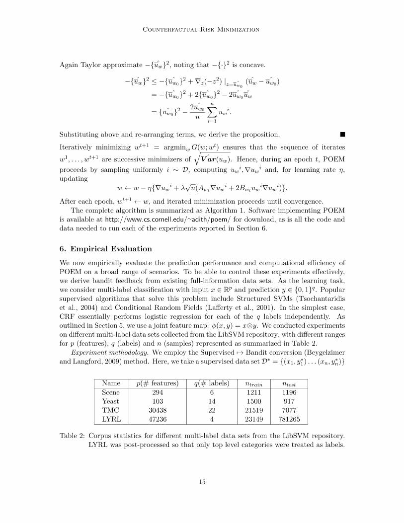
We now empirically evaluate the prediction performance and computational efficiency ofPOEM on a broad range of scenarios. To be able to control these experiments effectively,we derive bandit feedback from existing full-information data sets. As the learning task,we consider multi-label classification with input x ∈ Rp and prediction y ∈ {0, 1}q. Popularsupervised algorithms that solve this problem include Structured SVMs (Tsochantaridiset al., 2004) and Conditional Random Fields (Lafferty et al., 2001). In the simplest case,CRF essentially performs logistic regression for each of the q labels independently. Asoutlined in Section 5, we use a joint feature map: φ(x, y) = x⊗y. We conducted experimentson different multi-label data sets collected from the LibSVM repository, with different rangesfor p (features), q (labels) and n (samples) represented as summarized in Table 2.

Experiment methodology. We employ the Supervised 7→ Bandit conversion (Beygelzimerand Langford, 2009) method. Here, we take a supervised data setD∗ = {(x1, y∗1) . . . (xn, y

∗n)}

Name p(# features) q(# labels) ntrain ntestScene 294 6 1211 1196Yeast 103 14 1500 917TMC 30438 22 21519 7077LYRL 47236 4 23149 781265

Table 2: Corpus statistics for different multi-label data sets from the LibSVM repository.LYRL was post-processed so that only top level categories were treated as labels.

15

http://www.cs.cornell.edu/~adith/poem/

http://www.csie.ntu.edu.tw/~cjlin/libsvmtools/datasets/multilabel.html


Algorithm 1 POEM pseudocode. An alternative version can use separate samplers forestimating uw

i and {uwi}2 on Line 24.

1: procedure LossGradient(Ds, ~w) . Returns uwi,∇w(uw

i) for i ∈ Ds2: for i ∈ Ds do3: ui ← uw

i. . Equation (13)4: gi ← ∇w(uw

i).return ~u,~g.

5: procedure ABC(D, ~w, λ) . Returns Aw, Bw, Cw from Proposition (4)6: ~u,~g ← LossGradient(D, ~w).7: R←

∑i∈D ui/n.

8: V ←√∑

i∈D(ui −R)2/(n− 1).

9: A← 1− λ√nR

(n−1)V .

10: B ← λ2(n−1)V

√n

.

11: C ← λV2√n

+ λ√nR2

2(n−1)V .

return A,B,C.

12: procedure SGD(D, λ, µ) . L2 regularizer µ13: ~w ← [0]d. . Initial param

14: ~h← [1]d. . Adagrad history15: while True do16: Shuffle D.17: A,B,C ← ABC(D, w, λ).18: for Ds ⊂ D do . Minibatch |Ds| = b19: ~u,~g ← LossGradient(Ds, ~w).20: u =

∑i∈Ds ui/|Ds|.

21: g =∑

i∈Ds gi/|Ds|.22: hi ← hi + gi

2.23: ji ← gi/

√hi.

24: ~∇ ← A~j + 2µ~w + 2Bu~j.25: if ‖~∇‖ ' 0 then return ~w. . Gradient norm convergence

26: if u > avg u then return ~w. . Progressive validation

27: ~w ← ~w − η~∇. . Step size η

and simulate a bandit feedback data set from a logging policy h0 by sampling yi ∼ h0(xi)and collecting feedback ∆(y∗i , yi). In principle, we could use any arbitrary stochastic policyas h0. We choose a CRF trained on 5% of D∗ as h0 using default hyper-parameters, sincethey provide probability distributions amenable to sampling. In all the multi-label experi-ments, ∆(y∗, y) is the Hamming loss between the supervised label y∗ vs. the sampled label yfor input x. Hamming loss is just the number of incorrectly assigned labels (both false posi-tives and false negatives). To create bandit feedback D = {(xi, yi, δi ≡ ∆(y∗i , yi), pi ≡ h0(yi |xi))}, we take four passes through D∗ and sample labels from h0. Note that each supervisedlabel is worth ' |Y| = 2q bandit feedback labels. We can explore different learning strategies(e.g., IPS, CRM, etc.) on D and obtain learnt weight vectors wips, wcrm, etc. On the super-

16


vised test set, we then report the expected loss per instance R = 1ntest

∑i Ey∼hw(xi)∆(y∗i , y)

and compare the generalization error of these learning strategies.

Baselines and learning methods. The expected Hamming loss of h0 is the baseline tobeat. Lower loss is better. The naıve, variance-agnostic approach to counterfactual learning(Bottou et al., 2013; Strehl et al., 2010) can be generalized to handle parametric multilabelclassification by optimizing Equation (12) with λ = 0. We optimize it either using L-BFGS(IPS(B)) or stochastic optimization (IPS(S)). POEM(S) uses our Iterative-Majorizationapproach to variance regularization as outlined in Section 5.3, while POEM(B) is a L-BFGSvariant. Finally, we report results from a supervised CRF as a skyline, despite its unfairadvantage of having access to the full-information examples.

We keep aside 25% of D as a validation set—we use the unbiased counterfactual estima-tor from Equation (1) for selecting hyper-parameters. λ = cλ∗, where λ∗ is the calibrationfactor from Section 4.4 and c ∈ {10−6, . . . , 1} in multiples of 10. The clipping constant Mis similarly set to the ratio of the 90%ile to the 10%ile propensity score observed in thetraining set of D. The reported results are not sensitive to this choice of M , any reasonablylarge clipping constant suffices (e.g. even a simple, problem independent choice of M = 100works well). When optimizing any objective over w, we always begin the optimization fromw = 0, which is equivalent to hw = uniform(Y). We use mini-batch AdaGrad (Duchiet al., 2011) with batch size = 100 and step size η = 1 to adapt our learning rates forthe stochastic approaches and use progressive validation (Blum et al., 1999) and gradientnorms to detect convergence. Finally, the entire experiment set-up is run 10 times (i.e. h0trained on randomly chosen 5% subsets, D re-created, and test set performance of differentapproaches collected) and we report the averaged test set expected error across runs.

6.1 Does variance regularization improve generalization?

Results are reported in Table 3. We statistically test the performance of POEM againstIPS (batch variants are paired together, and the stochastic variants are paired together)using a one-tailed paired difference t-test at significance level of 0.05 across 10 runs ofthe experiment, and find POEM to be significantly better than IPS on each data set andeach optimization variant. Furthermore, on all data sets POEM learns a hypothesis thatsubstantially improves over the performance of h0. This suggests that the CRM principleis practically useful for designing learning algorithms, and that the variance regularizer isindeed beneficial.

6.2 How computationally efficient is POEM?

Table 4 shows the time taken (in CPU seconds) to run each method on each data set,averaged over different validation runs when performing hyper-parameter grid search. Someof the timing results are skewed by outliers, e.g., when under very weak regularization,CRFs tend to take longer to converge. However, it is still clear that the stochastic variantsare able to recover good parameter settings in a fraction of the time of batch L-BFGSoptimization, and this is even more pronounced when the number of labels grows—therun-time is dominated by computation of Z(xi).

17


R Scene Yeast TMC LYRL

h0 1.543 5.547 3.445 1.463

IPS(B) 1.193 4.635 2.808 0.921POEM(B) 1.168 4.480 2.197 0.918

IPS(S) 1.519 4.614 3.023 1.118POEM(S) 1.143 4.517 2.522 0.996

CRF 0.659 2.822 1.189 0.222

Table 3: Test set Hamming loss, R for different approaches to multi-label classification ondifferent data sets, averaged over 10 runs. POEM is significantly better than IPSon each data set and each optimization variant (one-tailed paired difference t-testat significance level of 0.05).

Time(s) Scene Yeast TMC LYRL

IPS(B) 2.58 47.61 136.34 21.01IPS(S) 1.65 2.86 49.12 13.66

POEM(B) 75.20 94.16 949.95 561.12POEM(S) 4.71 5.02 276.13 120.09

CRF 4.86 3.28 99.18 62.93

Table 4: Average time in seconds for each validation run for different approaches to multi-label classification. CRF is implemented by scikit-learn (Pedregosa et al., 2011).On all data sets, stochastic approaches are much faster than batch gradients.

6.3 Can MAP predictions derived from stochastic policies perform well?

For the policies learnt by POEM as shown in Table 3, Table 5 reports the averaged per-formance of the deterministic predictor derived from them. For a learnt weight vector w,this simply amounts to applying Equation (11). In practice, this method of generatingpredictions can be substantially faster than sampling since computing the argmax does notrequire computation of the partition function Z(x) which can be expensive in structuredoutput prediction. From Table 5, we see that the loss of the deterministic predictor istypically not far from the loss of the stochastic policy, and often better.

6.4 How does generalization improve with size of D?

As we collect more data under h0, our generalization error bound indicates that predictionperformance should eventually approach that of the optimal hypothesis in the hypothesisspace. We can simulate n → ∞ by replaying the training data multiple times, collectingsamples y ∼ h0(x). In the limit, we would observe every possible y in the bandit feedbackdata set, since h0(x) has non-zero probability of exploring each prediction y. However,the learning rate may be slow, since the exponential model family has very thin tails, and

18


R Scene Yeast TMC LYRL

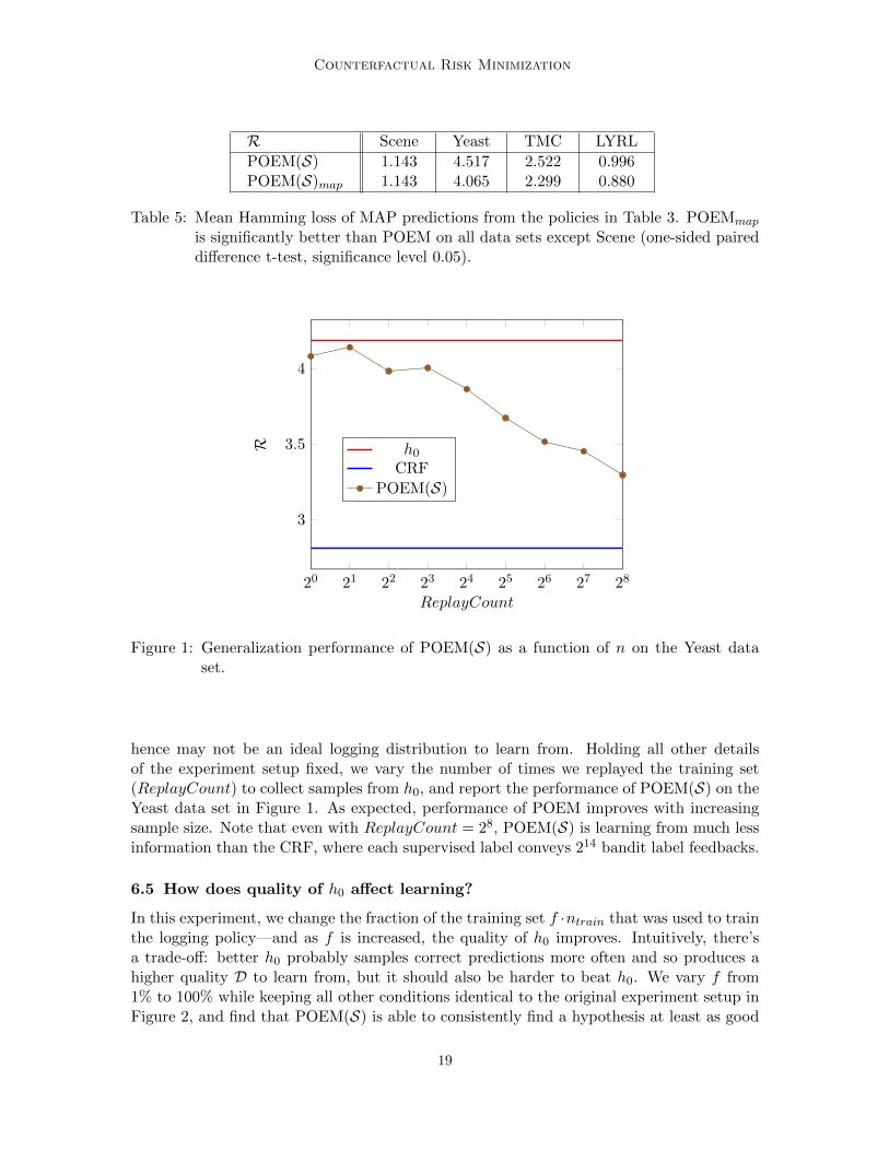
POEM(S) 1.143 4.517 2.522 0.996POEM(S)map 1.143 4.065 2.299 0.880

Table 5: Mean Hamming loss of MAP predictions from the policies in Table 3. POEMmap

is significantly better than POEM on all data sets except Scene (one-sided paireddifference t-test, significance level 0.05).

20 21 22 23 24 25 26 27 28

3

3.5

4

ReplayCount

R h0CRF

POEM(S)

Figure 1: Generalization performance of POEM(S) as a function of n on the Yeast dataset.

hence may not be an ideal logging distribution to learn from. Holding all other detailsof the experiment setup fixed, we vary the number of times we replayed the training set(ReplayCount) to collect samples from h0, and report the performance of POEM(S) on theYeast data set in Figure 1. As expected, performance of POEM improves with increasingsample size. Note that even with ReplayCount = 28, POEM(S) is learning from much lessinformation than the CRF, where each supervised label conveys 214 bandit label feedbacks.

6.5 How does quality of h0 affect learning?

In this experiment, we change the fraction of the training set f ·ntrain that was used to trainthe logging policy—and as f is increased, the quality of h0 improves. Intuitively, there’sa trade-off: better h0 probably samples correct predictions more often and so produces ahigher quality D to learn from, but it should also be harder to beat h0. We vary f from1% to 100% while keeping all other conditions identical to the original experiment setup inFigure 2, and find that POEM(S) is able to consistently find a hypothesis at least as good

19


0.2 0.4 0.6 0.8 1

4

5

6

f

R

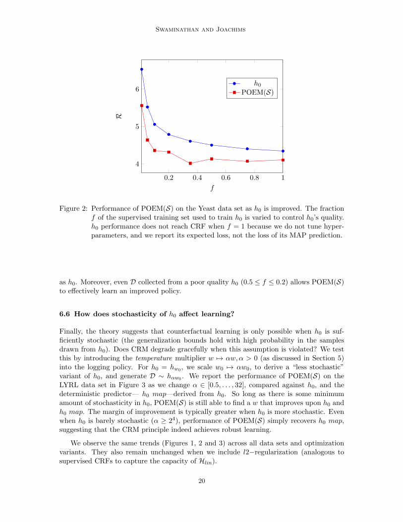
h0POEM(S)

Figure 2: Performance of POEM(S) on the Yeast data set as h0 is improved. The fractionf of the supervised training set used to train h0 is varied to control h0’s quality.h0 performance does not reach CRF when f = 1 because we do not tune hyper-parameters, and we report its expected loss, not the loss of its MAP prediction.

as h0. Moreover, even D collected from a poor quality h0 (0.5 ≤ f ≤ 0.2) allows POEM(S)to effectively learn an improved policy.

6.6 How does stochasticity of h0 affect learning?

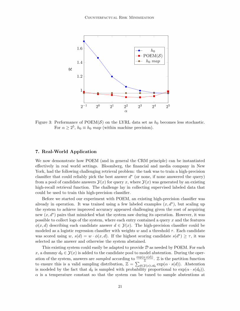
Finally, the theory suggests that counterfactual learning is only possible when h0 is suf-ficiently stochastic (the generalization bounds hold with high probability in the samplesdrawn from h0). Does CRM degrade gracefully when this assumption is violated? We testthis by introducing the temperature multiplier w 7→ αw,α > 0 (as discussed in Section 5)into the logging policy. For h0 = hw0 , we scale w0 7→ αw0, to derive a “less stochastic”variant of h0, and generate D ∼ hαw0 . We report the performance of POEM(S) on theLYRL data set in Figure 3 as we change α ∈ [0.5, . . . , 32], compared against h0, and thedeterministic predictor— h0 map—derived from h0. So long as there is some minimumamount of stochasticity in h0, POEM(S) is still able to find a w that improves upon h0 andh0 map. The margin of improvement is typically greater when h0 is more stochastic. Evenwhen h0 is barely stochastic (α ≥ 24), performance of POEM(S) simply recovers h0 map,suggesting that the CRM principle indeed achieves robust learning.

We observe the same trends (Figures 1, 2 and 3) across all data sets and optimizationvariants. They also remain unchanged when we include l2−regularization (analogous tosupervised CRFs to capture the capacity of Hlin).

20


2−1 20 21 22 23 24 25

1

1.2

1.4

1.6

α

R

h0POEM(S)h0 map

Figure 3: Performance of POEM(S) on the LYRL data set as h0 becomes less stochastic.For α ≥ 25, h0 ≡ h0 map (within machine precision).

7. Real-World Application

We now demonstrate how POEM (and in general the CRM principle) can be instantiatedeffectively in real world settings. Bloomberg, the financial and media company in NewYork, had the following challenging retrieval problem: the task was to train a high-precisionclassifier that could reliably pick the best answer d∗ (or none, if none answered the query)from a pool of candidate answers Y(x) for query x, where Y(x) was generated by an existinghigh-recall retrieval function. The challenge lay in collecting supervised labeled data thatcould be used to train this high-precision classifier.

Before we started our experiment with POEM, an existing high-precision classifier wasalready in operation. It was trained using a few labeled examples (x, d∗), but scaling upthe system to achieve improved accuracy appeared challenging given the cost of acquiringnew (x, d∗) pairs that mimicked what the system saw during its operation. However, it waspossible to collect logs of the system, where each entry contained a query x and the featuresφ(x, d) describing each candidate answer d ∈ Y(x). The high-precision classifier could bemodeled as a logistic regression classifier with weights w and a threshold τ . Each candidatewas scored using w, s(d) = w · φ(x, d). If the highest scoring candidate s(d∗) ≥ τ , it wasselected as the answer and otherwise the system abstained.

This existing system could easily be adapted to provide D as needed by POEM. For eachx, a dummy d0 ∈ Y(x) is added to the candidate pool to model abstention. During the oper-

ation of the system, answers are sampled according to exp(α·s(d))Z . Z is the partition function

to ensure this is a valid sampling distribution, Z =∑

d∈Y(x)∪d0 exp(α · s(d)). Abstentionis modeled by the fact that d0 is sampled with probability proportional to exp(α · s(d0)).α is a temperature constant so that the system can be tuned to sample abstentions at

21


roughly the same rate as its deterministic counterpart. Finally, the end-result feedback(δ ∈ {thumbs-up, thumbs-down} represented as binary feedback) was logged and providedbandit feedback for the presented answer d.

This data set was much easier to collect during the system run compared to annotatingeach x in the logs with the best possible d∗ that would have answered the query. We arguethat this is a general, practical, alternative approach to training retrieval systems: use anystrategy with very high recall to construct Y, then use the parameters w estimated usingthe CRM principle to search through this Y and find a precise answer.

On a small pilot study, we acquired D with ' 4000 (x, d, exp(α·s(d))Z , δ) tuples in thetraining set and ' 500 tuples in the validation and test sets. We verified that the existinghigh-precision classifier was statistically significantly better than random baselines for theproblem. POEM(S) is trained on this log data by performing gradient descent with winitialized to w0 = 0 and validating c ∈

[10−6, . . . 1

], λ = cλ∗ as described in Sections 4.4

and 6. POEM(S) found a w∗ that improved δ feedback over the existing system by over30%, as estimated using the unbiased counterfactual estimator of Equation (1) on the testset. Without using the variance regularizer, the IPS(S) found a w∗ that degraded thesystem performance by 3.5% estimated counterfactually in the same way. This shows thatPOEM and the CRM principle can bring potential benefit even in binary-feedback multi-class classification settings where classic supervised learning approaches lack available data.

8. Conclusion

Counterfactual risk minimization serves as a robust principle for designing algorithms thatcan learn from a batch of bandit feedback interactions. The key insight for CRM is toexpand the classical notion of a hypothesis class to include stochastic policies, reason aboutvariance in the risk estimator, and derive a generalization error bound over this hypothesisspace. The practical take-away is a simple, data-dependent regularizer that guaranteesrobust learning. Following the CRM principle, we developed the POEM learning algorithmfor structured output prediction. POEM can optimize over rich policy families (exponentialmodels corresponding to linear rules in supervised learning), and deal with massive outputspaces as efficiently as classical supervised methods.

The CRM principle more generally applies to supervised learning with non-differentiablelosses, since the objective does not require the gradient of the loss function. We also foreseeextensions of the algorithm to handle ordinal or co-active feedback models for δ(·, ·), andextensions of the generalization error bound to include adaptive or deterministic h0, etc.

Acknowledgments

This research was funded in part through NSF Awards IIS-1247637, IIS-1217686, IIS-1513692, the JTCII Cornell-Technion Research Fund, and a gift from Bloomberg.

22


References

Martin Anthony and Peter L. Bartlett. Neural Network Learning: Theoretical Foundations.Cambridge University Press, New York, NY, USA, 2009.

Alina Beygelzimer and John Langford. The offset tree for learning with partial labels. InProceedings of the 15th ACM SIGKDD International Conference on Knowledge Discoveryand Data Mining, pages 129–138, 2009.

Avrim Blum, Adam Kalai, and John Langford. Beating the hold-out: Bounds for k-foldand progressive cross-validation. In Proceedings of the Twelfth Annual Conference onComputational Learning Theory, pages 203–208, 1999.

Leon Bottou, Jonas Peters, Joaquin Q. Candela, Denis X. Charles, Max Chickering, ElonPortugaly, Dipankar Ray, Patrice Y. Simard, and Ed Snelson. Counterfactual reasoningand learning systems: the example of computational advertising. Journal of MachineLearning Research, 14(1):3207–3260, 2013.

Corinna Cortes, Yishay Mansour, and Mehryar Mohri. Learning bounds for importanceweighting. In Proceedings of the 23rd Annual Conference on Neural Information Process-ing Systems, pages 442–450, 2010.

John Duchi, Elad Hazan, and Yoram Singer. Adaptive subgradient methods for onlinelearning and stochastic optimization. Journal of Machine Learning Research, 12:2121–2159, 2011.

Miroslav Dudık, John Langford, and Lihong Li. Doubly robust policy evaluation and learn-ing. In Proceedings of the 28th International Conference on Machine Learning, pages1097–1104, 2011.

Nicolas Galichet, Michele Sebag, and Olivier Teytaud. Exploration vs exploitation vs safety:Risk-aware multi-armed bandits. In Asian Conference on Machine Learning, pages 245–260, 2013.

J. Garcia and F. Fernandez. Safe exploration of state and action spaces in reinforcementlearning. Journal of Artificial Intelligence Research, 45:515–564, 2012.

Katja Hofmann, Anne Schuth, Shimon Whiteson, and Maarten de Rijke. Reusing historicalinteraction data for faster online learning to rank for IR. In Sixth ACM InternationalConference on Web Search and Data Mining, pages 183–192, 2013.

Edward L. Ionides. Truncated importance sampling. Journal of Computational and Graph-ical Statistics, 17(2):295–311, 2008.

John D. Lafferty, Andrew McCallum, and Fernando C. N. Pereira. Conditional randomfields: Probabilistic models for segmenting and labeling sequence data. In Proceedings ofthe 18th International Conference on Machine Learning, pages 282–289, 2001.

John Langford and Tong Zhang. The epoch-greedy algorithm for multi-armed bandits withside information. In Proceedings of the 21st Annual Conference on Neural InformationProcessing Systems, pages 817–824, 2008.

23


John Langford, Alexander Strehl, and Jennifer Wortman. Exploration scavenging. InProceedings of the 25th International Conference on Machine Learning, pages 528–535,2008.

Adrian S. Lewis and Michael L. Overton. Nonsmooth optimization via quasi-newton meth-ods. Mathematical Programming, 141(1-2):135–163, 2013.

Lihong Li, Wei Chu, John Langford, and Robert E. Schapire. A contextual-bandit approachto personalized news article recommendation. In Proceedings of the 19th InternationalConference on World Wide Web, pages 661–670, 2010.

Lihong Li, Wei Chu, John Langford, and Xuanhui Wang. Unbiased offline evaluation ofcontextual-bandit-based news article recommendation algorithms. In Proceedings of the4th ACM International Conference on Web Search and Data Mining, pages 297–306,2011.

Lihong Li, Shunbao Chen, Jim Kleban, and Ankur Gupta. Counterfactual estimation andoptimization of click metrics for search engines. CoRR, abs/1403.1891, 2014.

Lihong Li, Remi Munos, and Csaba Szepesvari. Toward minimax off-policy value estima-tion. In Proceedings of the 18th International Conference on Artificial Intelligence andStatistics (AISTATS), 2015.

Jeremie Mary, Philippe Preux, and Olivier Nicol. Improving offline evaluation of contextualbandit algorithms via bootstrapping techniques. In Proceedings of the 31st InternationalConference on Machine Learning, pages 172–180, 2014.

Andreas Maurer and Massimiliano Pontil. Empirical bernstein bounds and sample-variancepenalization. In Proceedings of the 22nd Conference on Learning Theory, 2009.

Art B. Owen. Monte Carlo theory, methods and examples. 2013.

F. Pedregosa, G. Varoquaux, A. Gramfort, V. Michel, B. Thirion, O. Grisel, M. Blon-del, P. Prettenhofer, R. Weiss, V. Dubourg, J. Vanderplas, A. Passos, D. Cournapeau,M. Brucher, M. Perrot, and E. Duchesnay. Scikit-learn: Machine learning in Python.Journal of Machine Learning Research, 12:2825–2830, 2011.

Paul R. Rosenbaum and Donald B. Rubin. The central role of the propensity score inobservational studies for causal effects. Biometrika, 70(1):41–55, 1983.

Pannagadatta K. Shivaswamy and Thorsten Joachims. Multi-armed bandit problems withhistory. In Proceedings of the 15th International Conference on Artificial Intelligence andStatistics, pages 1046–1054, 2012.

Alexander L. Strehl, John Langford, Lihong Li, and Sham Kakade. Learning from loggedimplicit exploration data. In Proceedings of the 24th Annual Conference on Neural In-formation Processing Systems, pages 2217–2225, 2010.

Adith Swaminathan and Thorsten Joachims. Counterfactual risk minimization: Learningfrom logged bandit feedback. In Proceedings of the 32nd International Conference onMachine Learning, 2015.

24


Philip S. Thomas, Georgios Theocharous, and Mohammad Ghavamzadeh. High-confidenceoff-policy evaluation. In Proceedings of the 29th AAAI Conference on Artificial Intelli-gence, pages 3000–3006, 2015.

Ioannis Tsochantaridis, Thomas Hofmann, Thorsten Joachims, and Yasemin Altun. Supportvector machine learning for interdependent and structured output spaces. In Proceedingsof the 21st International Conference on Machine Learning, pages 104–, 2004.

G.J.J. van den Burg and P.J.F. Groenen. GenSVM: A Generalized Multiclass SupportVector Machine. Technical Report EI 2014-33, Erasmus University Rotterdam, ErasmusSchool of Economics (ESE), Econometric Institute, 2014.

W. N. Wapnik and A. J. Tscherwonenkis. Theorie der Zeichenerkennung. Akademie Verlag,Berlin, 1979.

Jin Yu, S. V. N. Vishwanathan, Simon Gunter, and Nicol N. Schraudolph. A quasi-Newtonapproach to nonsmooth convex optimization problems in machine learning. Journal ofMachine Learning Research, 11:1145–1200, 2010.

25

Documents

Batch Learning from Logged Bandit Feedback through ... Learning from Logged Bandit Feedback through Counterfactual Risk Minimization Adith Swaminathan [email protected] Department