Basis of Structural Analysis 0809 - Colin C. Caprani

Structural Analysis III

Dr. C. Caprani 1

Structural Analysis III Basis for the Analysis of

Indeterminate Structures

2008/9

Dr. Colin Caprani


Dr. C. Caprani 2

Contents 1. Introduction ......................................................................................................... 3

1.1 Background...................................................................................................... 3

1.2 Basis of Structural Analysis ............................................................................ 4

2. Small Displacements............................................................................................ 5

2.1 Introduction...................................................................................................... 5

2.2 Derivation ........................................................................................................ 6

2.3 Movement of Oblique Members ..................................................................... 9

2.4 Instantaneous Centre of Rotation .................................................................. 12

3. Compatibility of Displacements ....................................................................... 18

3.1 Description..................................................................................................... 18

3.2 Examples........................................................................................................ 19

4. Principle of Superposition ................................................................................ 21

4.1 Development.................................................................................................. 21

4.2 Example ......................................................................................................... 23

5. Solving Indeterminate Structures.................................................................... 24

5.1 Introduction.................................................................................................... 24

5.2 Example: Propped Cantilever........................................................................ 25

5.3 Example: 2-Span Beam ................................................................................. 27

6. Problems............................................................................................................. 29

7. Table of Displacements ..................................................................................... 30


Dr. C. Caprani 3

1. Introduction

1.1 Background

In the case of 2-dimensional structures there are three equations of statics:

0

0

0

x

y

F

F

M

=

=

=

∑∑∑

Thus only three unknowns (reactions etc.) can be solved for using these equations

alone. Structures that cannot be solved through the equations of static equilibrium

alone are known as statically indeterminate structures. These, then, are structures that

have more than 3 unknowns to be solved for. Therefore, in order to solve statically

indeterminate structures we must identify other knowns about the structure.


Dr. C. Caprani 4

1.2 Basis of Structural Analysis

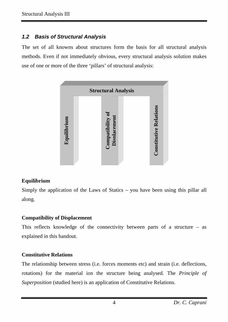
The set of all knowns about structures form the basis for all structural analysis

methods. Even if not immediately obvious, every structural analysis solution makes

use of one or more of the three ‘pillars’ of structural analysis:

Equilibrium

Simply the application of the Laws of Statics – you have been using this pillar all

along.

Compatibility of Displacement

This reflects knowledge of the connectivity between parts of a structure – as

explained in this handout.

Constitutive Relations

The relationship between stress (i.e. forces moments etc) and strain (i.e. deflections,

rotations) for the material ion the structure being analysed. The Principle of

Superposition (studied here) is an application of Constitutive Relations.

Equ

ilibr

ium

Con

stitu

tive

Rel

atio

ns

Com

patib

ility

of

Dis

plac

emen

t

Structural Analysis


Dr. C. Caprani 5

2. Small Displacements

2.1 Introduction

In structural analysis we will often make the assumption that displacements are small.

This allows us to use approximations for displacements that greatly simplify analysis.

What do we mean by small displacements?

We take small displacements to be such that the arc and chord length are

approximately equal. This will be explained further on.

Is it realistic?

Yes – most definitely. Real structures deflect very small amounts. For example,

sways are usually limited to storey height over 500. Thus the arc or chord length is of

the order 1/500th of the radius (or length of the member which is the storey height).

As will be seen further on, such a small rotation allows the use of the approximation

of small displacement.

Lastly, but importantly, in the analysis of flexural members, we ignore any changes

in lengths of members due to axial loads. That is:

We neglect axial deformations – members do not change length.

This is because such members have large areas (as required for bending resistance)

and so have negligible elastic shortening.


Dr. C. Caprani 6

2.2 Derivation

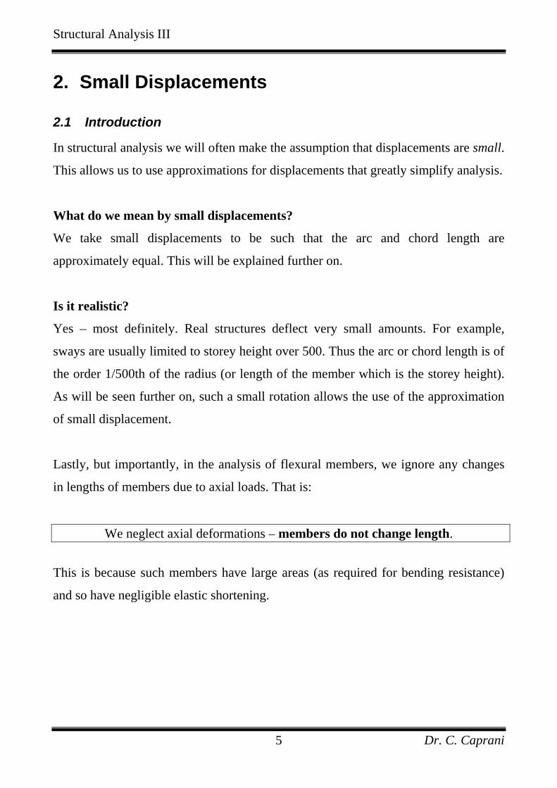
Remember – all angles are in radians.

Consider a member AB, of length R, that rotates about A, an amount θ , to a new

position B’ as shown:

The total distance travelled by the point B is the length of the arc BB’, which is Rθ .

There is also the ‘perpendicular distance’ travelled by B: CB’. Obviously:

' '

Chord Length Arc Lengthtan

CB BB

R Rθ θ

<

<<


Dr. C. Caprani 7

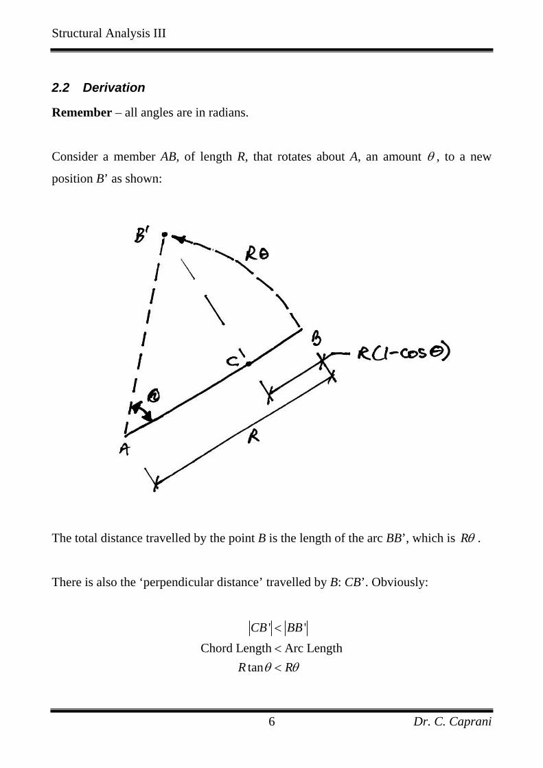
There is also a movement of B along the line AB: BC, which has a length of:

( )1 cosR θ−

Now if we consider a ‘small’ displacement of point B:

We can see now that the arc and chord lengths must be almost equal and so we use

the approximation:

' tanBB R Rθ θ= ≈

This is the approximation inherent in a lot of basic structural analysis. There are

several things to note:

• It relies on the assumption that tanθ θ≈ for small angles;

• There is virtually no movement along the line of the member, i.e.

( )1 cos 0R θ− ≈ and so we neglect the small notional increase in length

'AB ABδ = − shown above.


Dr. C. Caprani 8

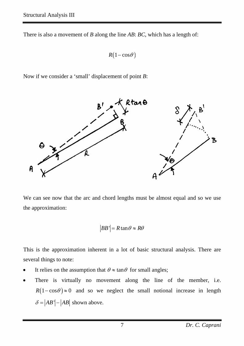
A graph of the arc and chord lengths for some angles is:

0

0.1

0.2

0.3

0.4

0.5

0.6

0.7

0 5 10 15 20 25 30Angle (Degrees)

Dis

tanc

e M

oved

ChordArc

For usual structural movements (as represented by deflection limits), the difference

between the arc and chord length approximation is:

0

0.05

0.1

0.15

0.2

0.25

1 10 100 1000Deflection Limit (h/?)

Arc

h &

Cho

rd D

iffer

ence

Since even the worst structural movement is of the order 200h there is negligible

difference between the arc and chord lengths and so the approximation of small

angles holds.


Dr. C. Caprani 9

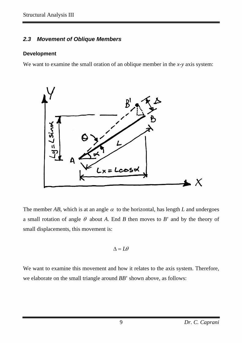
2.3 Movement of Oblique Members

Development

We want to examine the small oration of an oblique member in the x-y axis system:

The member AB, which is at an angle α to the horizontal, has length L and undergoes

a small rotation of angle θ about A. End B then moves to B’ and by the theory of

small displacements, this movement is:

Lθ∆ =

We want to examine this movement and how it relates to the axis system. Therefore,

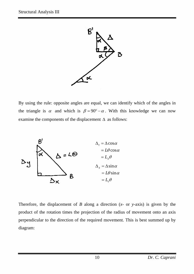
we elaborate on the small triangle around BB’ shown above, as follows:


Dr. C. Caprani 10

By using the rule: opposite angles are equal, we can identify which of the angles in

the triangle is α and which is 90β α= ° − . With this knowledge we can now

examine the components of the displacement ∆ as follows:

coscos

Y

X

LL

αθ αθ

∆ = ∆==

sinsin

X

Y

LL

αθ αθ

∆ = ∆==

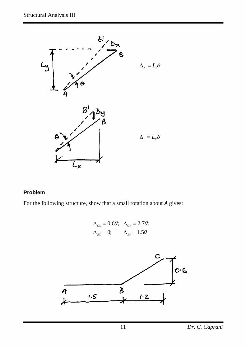
Therefore, the displacement of B along a direction (x- or y-axis) is given by the

product of the rotation times the projection of the radius of movement onto an axis

perpendicular to the direction of the required movement. This is best summed up by

diagram:


Dr. C. Caprani 11

X YL θ∆ =

Y XL θ∆ =

Problem

For the following structure, show that a small rotation about A gives:

0.6 ; 2.7 ;0; 1.5

CX CY

BX BY

θ θθ

∆ = ∆ =∆ = ∆ =


Dr. C. Caprani 12

2.4 Instantaneous Centre of Rotation

Definition

For assemblies of members (i.e. structures), individual members movements are not

separable from that of the structure. A ‘global’ view of the movement of the structure

can be achieved using the concept of the Instantaneous Centre of Rotation (ICR).

The Instantaneous Centre of Rotation is the point about which, for any given moment

in time, the rotation of a body is occurring. It is therefore the only point that is not

moving. In structures, each member can have its own ICR. However, movement of

the structure is usually defined by an obvious ICR.


Dr. C. Caprani 13

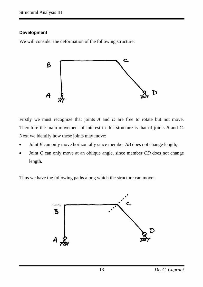
Development

We will consider the deformation of the following structure:

Firstly we must recognize that joints A and D are free to rotate but not move.

Therefore the main movement of interest in this structure is that of joints B and C.

Next we identify how these joints may move:

• Joint B can only move horizontally since member AB does not change length;

• Joint C can only move at an oblique angle, since member CD does not change

length.

Thus we have the following paths along which the structure can move:


Dr. C. Caprani 14

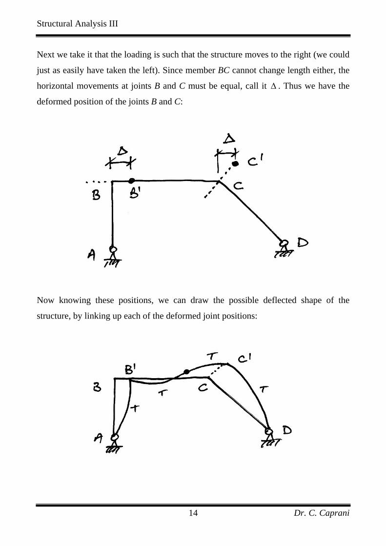
Next we take it that the loading is such that the structure moves to the right (we could

just as easily have taken the left). Since member BC cannot change length either, the

horizontal movements at joints B and C must be equal, call it ∆ . Thus we have the

deformed position of the joints B and C:

Now knowing these positions, we can draw the possible deflected shape of the

structure, by linking up each of the deformed joint positions:


Dr. C. Caprani 15

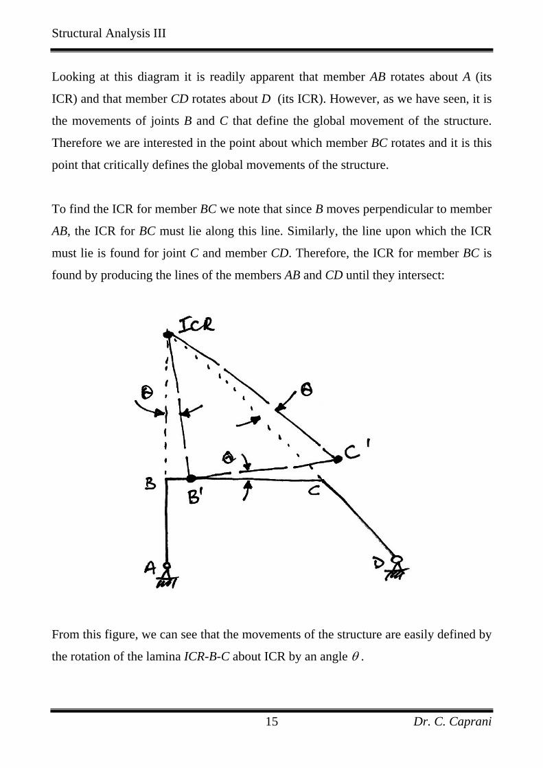
Looking at this diagram it is readily apparent that member AB rotates about A (its

ICR) and that member CD rotates about D (its ICR). However, as we have seen, it is

the movements of joints B and C that define the global movement of the structure.

Therefore we are interested in the point about which member BC rotates and it is this

point that critically defines the global movements of the structure.

To find the ICR for member BC we note that since B moves perpendicular to member

AB, the ICR for BC must lie along this line. Similarly, the line upon which the ICR

must lie is found for joint C and member CD. Therefore, the ICR for member BC is

found by producing the lines of the members AB and CD until they intersect:

From this figure, we can see that the movements of the structure are easily defined by

the rotation of the lamina ICR-B-C about ICR by an angle θ .


Dr. C. Caprani 16

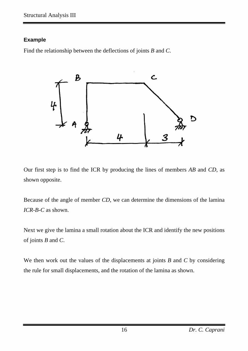
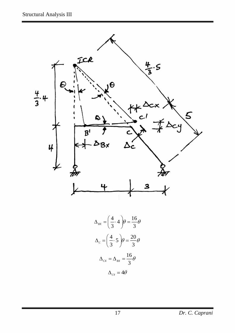
Example

Find the relationship between the deflections of joints B and C.

Our first step is to find the ICR by producing the lines of members AB and CD, as

shown opposite.

Because of the angle of member CD, we can determine the dimensions of the lamina

ICR-B-C as shown.

Next we give the lamina a small rotation about the ICR and identify the new positions

of joints B and C.

We then work out the values of the displacements at joints B and C by considering

the rule for small displacements, and the rotation of the lamina as shown.


Dr. C. Caprani 17

4 1643 3BX θ θ⎛ ⎞∆ = ⋅ =⎜ ⎟

⎝ ⎠

4 2053 3C θ θ⎛ ⎞∆ = ⋅ =⎜ ⎟

⎝ ⎠

163CX BX θ∆ = ∆ =

4CY θ∆ =


Dr. C. Caprani 18

3. Compatibility of Displacements

3.1 Description

When a structure is loaded it deforms under that load. Points that were connected to

each other remain connected to each other, though the distance between them may

have altered due to the deformation. All the points in a structure do this is such a way

that the structure remains fitted together in its original configuration.

Compatibility of displacement is thus:

Displacements are said to be compatible when the deformed members of a

loaded structure continue to fit together.

Thus, compatibility means that:

• Two initially separate points do not move to another common point;

• Holes do not appear as a structure deforms;

• Members initially connected together remain connected together.

This deceptively simple idea is very powerful when applied to indeterminate

structures.


Dr. C. Caprani 19

3.2 Examples

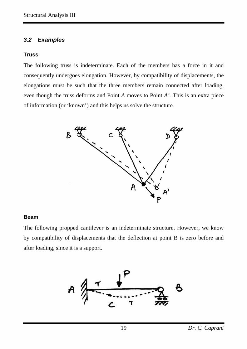
Truss

The following truss is indeterminate. Each of the members has a force in it and

consequently undergoes elongation. However, by compatibility of displacements, the

elongations must be such that the three members remain connected after loading,

even though the truss deforms and Point A moves to Point A’. This is an extra piece

of information (or ‘known’) and this helps us solve the structure.

Beam

The following propped cantilever is an indeterminate structure. However, we know

by compatibility of displacements that the deflection at point B is zero before and

after loading, since it is a support.


Dr. C. Caprani 20

Frame

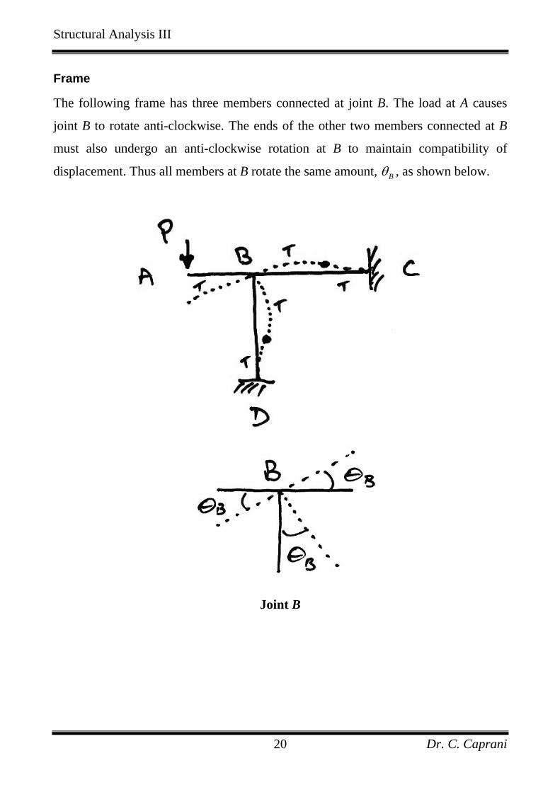
The following frame has three members connected at joint B. The load at A causes

joint B to rotate anti-clockwise. The ends of the other two members connected at B

must also undergo an anti-clockwise rotation at B to maintain compatibility of

displacement. Thus all members at B rotate the same amount, Bθ , as shown below.

Joint B


Dr. C. Caprani 21

4. Principle of Superposition

4.1 Development

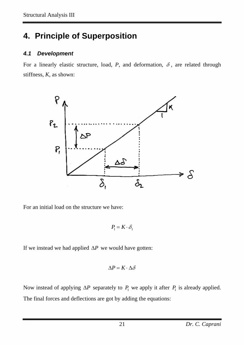
For a linearly elastic structure, load, P, and deformation, δ , are related through

stiffness, K, as shown:

For an initial load on the structure we have:

1 1P K δ= ⋅

If we instead we had applied P∆ we would have gotten:

P K δ∆ = ⋅∆

Now instead of applying P∆ separately to 1P we apply it after 1P is already applied.

The final forces and deflections are got by adding the equations:


Dr. C. Caprani 22

( )

1 1

1

P P K KK

δ δδ δ

+ ∆ = ⋅ + ⋅∆

= + ∆

But, since from the diagram, 2 1P P P= + ∆ and 2 1δ δ δ= + ∆ , we have:

2 2P K δ= ⋅

which is a result we expected.

This result, though again deceptively ‘obvious’, tells us that:

• Deflection caused by a force can be added to the deflection caused by another

force to get the deflection resulting from both forces being applied;

• The order of loading is not important ( P∆ or 1P could be first);

• Loads and their resulting load effects can be added or subtracted for a

structure.

This is the Principle of Superposition:

For a linearly elastic structure, the load effects caused by two or more

loadings are the sum of the load effects caused by each loading separately.

Note that the principle is limited to:

• Linear material behaviour only;

• Structures undergoing small deformations only (linear geometry).


Dr. C. Caprani 23

4.2 Example

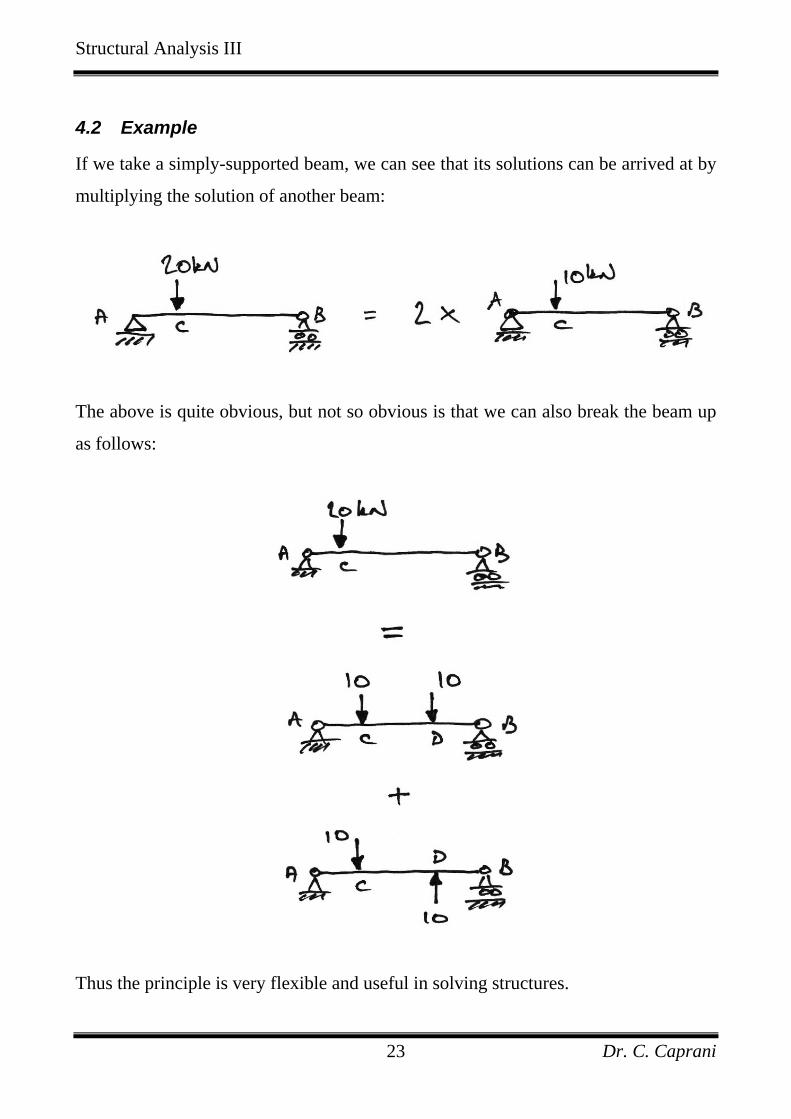
If we take a simply-supported beam, we can see that its solutions can be arrived at by

multiplying the solution of another beam:

The above is quite obvious, but not so obvious is that we can also break the beam up

as follows:

Thus the principle is very flexible and useful in solving structures.


Dr. C. Caprani 24

5. Solving Indeterminate Structures

5.1 Introduction

Compatibility of displacement along with superposition enables us to solve

indeterminate structures. Though we’ll use more specialized techniques they will be

fundamentally based upon the preceding ideas. Some simple example applications

follow.


Dr. C. Caprani 25

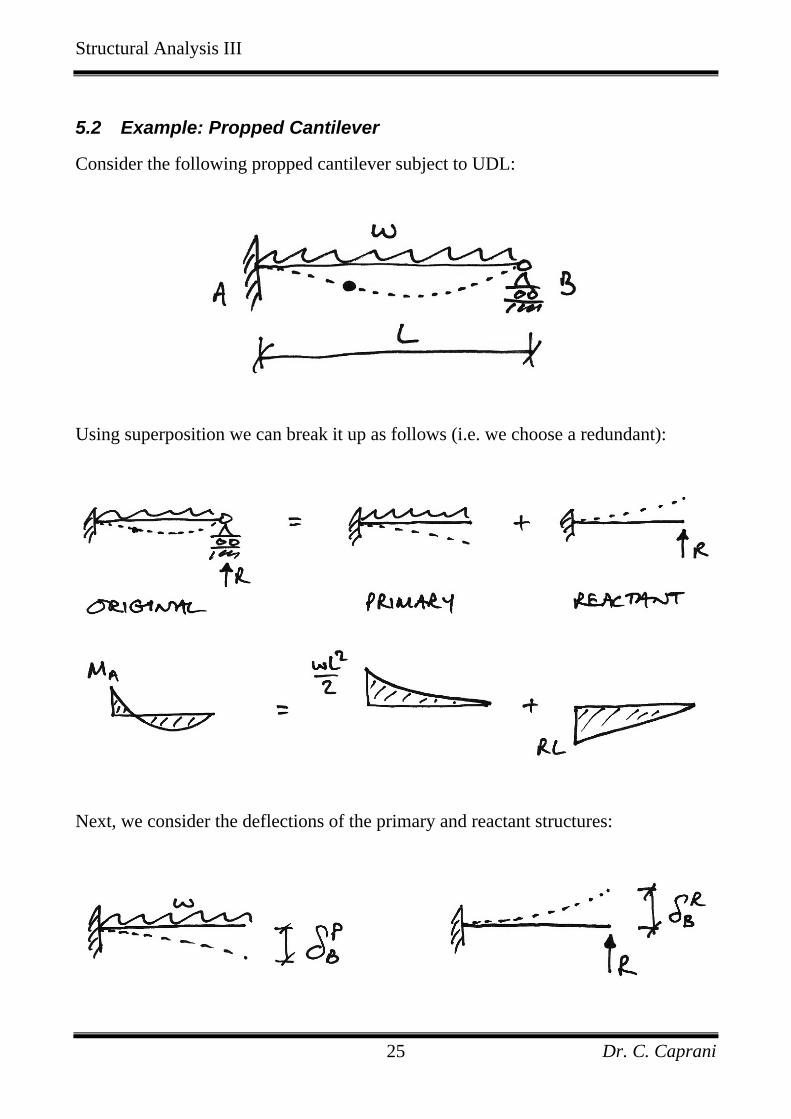
5.2 Example: Propped Cantilever

Consider the following propped cantilever subject to UDL:

Using superposition we can break it up as follows (i.e. we choose a redundant):

Next, we consider the deflections of the primary and reactant structures:


Dr. C. Caprani 26

Now by compatibility of displacements for the original structure, we know that we

need to have a final deflection of zero after adding the primary and reactant

deflections at B:

0P RB B Bδ δ δ= + =

From tables of standard deflections, we have:

4 3

and 8 3

P RB B

wL RLEI EI

δ δ= + = −

In which downwards deflections are taken as positive. Thus we have:

4 3

08 33

8

BwL RLEI EIwLR

δ = + − =

∴ =

Knowing this, we can now solve for any other load effect. For example:

2

2

2 2

2

23

2 84 3

8

8

AwLM RL

wL wL L

wL wL

wL

= −

= −

−=

=

Note that the 2 8wL term arises without a simply-supported beam in sight!


Dr. C. Caprani 27

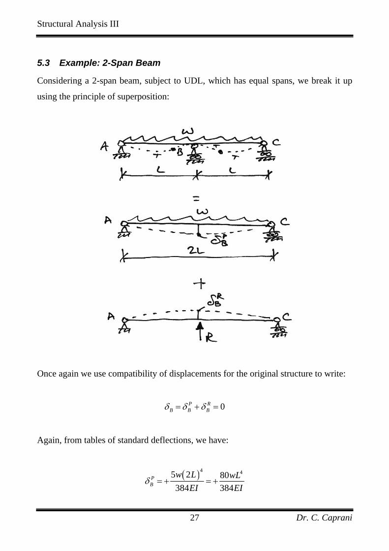
5.3 Example: 2-Span Beam

Considering a 2-span beam, subject to UDL, which has equal spans, we break it up

using the principle of superposition:

Once again we use compatibility of displacements for the original structure to write:

0P RB B Bδ δ δ= + =

Again, from tables of standard deflections, we have:

( )4 45 2 80384 384

PB

w L wLEI EI

δ = + = +


Dr. C. Caprani 28

And:

( )3 32 848 48

RB

R L RLEI EI

δ = − = −

In which downwards deflections are taken as positive. Thus we have:

4 380 8 0384 48

8 8048 384

108

BwL RL

EI EIR wL

wLR

δ = + − =

=

=

Note that this is conventionally not reduced to 5 4wL since the other reactions are

both 3 8wL . Show this as an exercise.

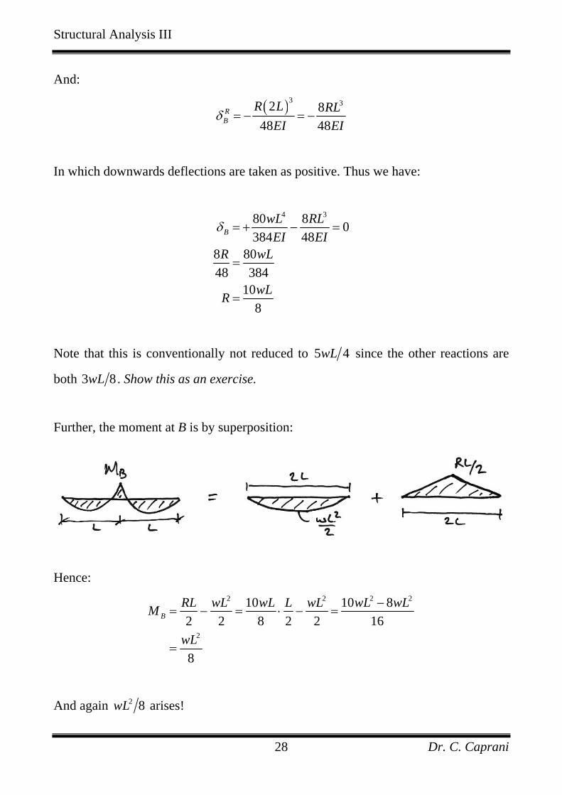
Further, the moment at B is by superposition:

Hence:

2 2 2 2

2

10 10 82 2 8 2 2 16

8

BRL wL wL L wL wL wLM

wL

−= − = ⋅ − =

=

And again 2 8wL arises!


Dr. C. Caprani 29

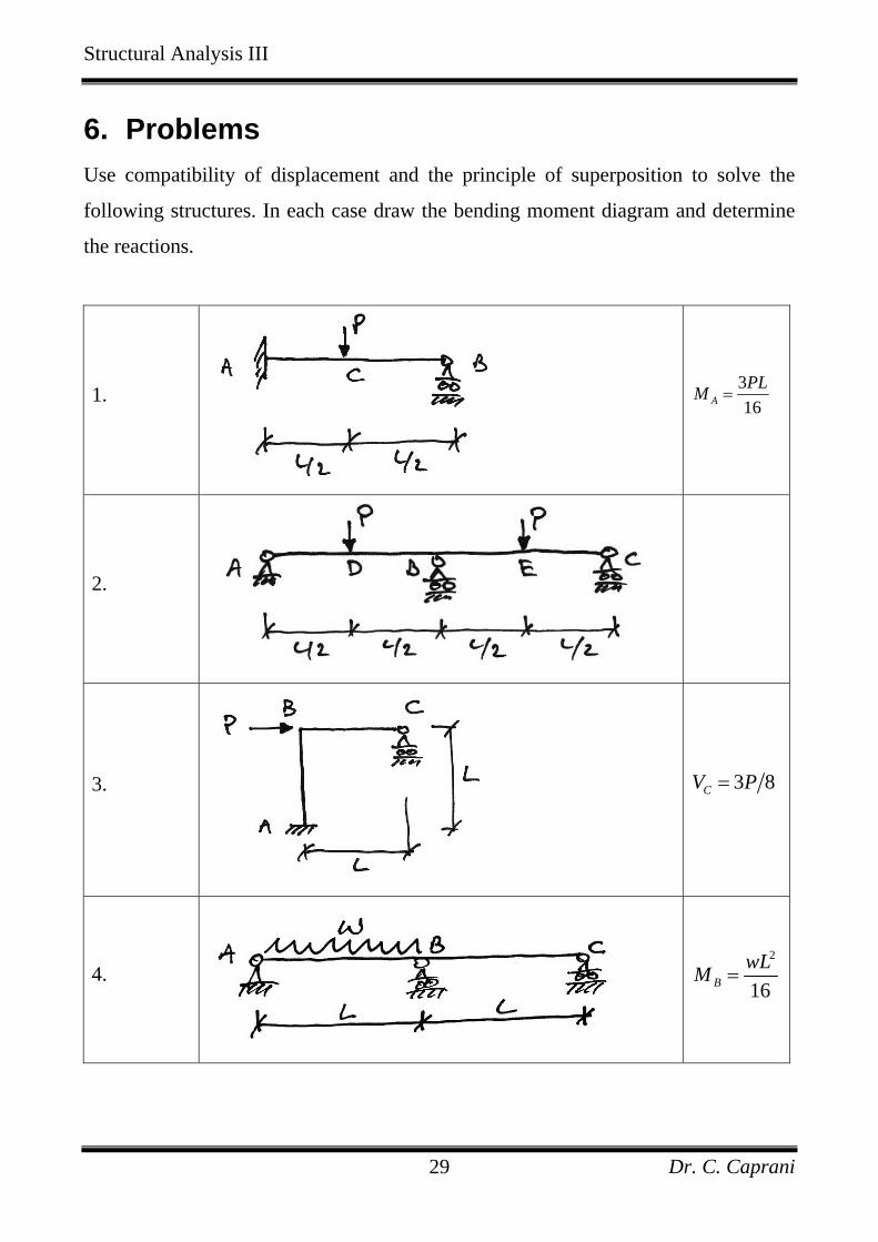
6. Problems Use compatibility of displacement and the principle of superposition to solve the

following structures. In each case draw the bending moment diagram and determine

the reactions.

1.

316APLM =

2.

3.

3 8CV P=

4.

2

16BwLM =


Dr. C. Caprani 30

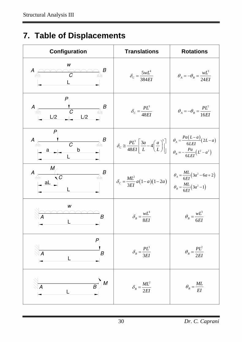
7. Table of Displacements

Configuration Translations Rotations

w

L

A BC

45384C

wLEI

δ = 3

24A BwL

EIθ θ= − =

P

L/2 L/2

A BC

3

48CPL

EIδ =

2

16A BPL

EIθ θ= − =

P

a bL

A BC

33 3 448CPL a a

EI L Lδ

⎡ ⎤⎛ ⎞≅ −⎢ ⎥⎜ ⎟⎝ ⎠⎢ ⎥⎣ ⎦

( ) ( )

( )2 2

26

6

A

B

Pa L aL a

LEIPa L aLEI

θ

θ

−= −

= − −

aLL

A BC

( )( )2

1 1 23CML a a a

EIδ = − −

( )

( )

2

2

3 6 26

3 16

A

B

ML a aEI

ML aEI

θ

θ

= − +

= −

w

LA B

4

8BwLEI

δ = 3

6BwLEI

θ =

P

LA B

3

3BPLEI

δ = 2

2BPLEI

θ =

LA B

M

2

2BML

EIδ = B

MLEI

θ =

Documents

Basis of Structural Analysis 0809 - Colin C. Caprani