Embed Size (px)
Citation preview
Comenius UniversityFaculty of Mathematics, Physics and Informatics
Department of Astronomy, Physics of the Earth, and Meteorology
( KAFZM FMFI UK )
Peter Moczo
Basics of Continuum Mechanics
( unpublished lecture notes for students of geophysics )
Bratislava 2001, 2006

c©Peter Moczo 2001, 2006
Preface
These notes only reproduce the first chapter of Introduction to Theoretical Seismology.This file was created for convenience of those who are not interested in seismology and only wantto learn basic concepts of continuum mechanics. As in the preface to Introduction to Theo-retical Seismology I want to stress that the notes are just transcription of what I originallyhand-wrote on transparencies for students of the course Theory of Seismic Waves at Univer-sitat Wien in 2001. In other words, the material was not and is not intended as a standardintroductory text on the topic.
The material is mainly based on the book by Aki and Richards (1980, 2002).I want to acknowledge help from Peter Pazak as well as technical assistance of Martin Minka
and Lenka Molnarova.
Table of Contents
Preface . . . . . . . . . . . . . . . . . . . . . . . . . . . . . . . . . . . . . . . . . . . . . . . . . . . . . . . . . . . . . . . . . . . . . . . . i
1. BASIC RELATIONS OF CONTINUUM MECHANICS . . . . . . . . . . . . . . . . . . . 11.1 Introduction . . . . . . . . . . . . . . . . . . . . . . . . . . . . . . . . . . . . . . . . . . . . . . . . . . . . . . . . . . . . . 11.2 Body forces . . . . . . . . . . . . . . . . . . . . . . . . . . . . . . . . . . . . . . . . . . . . . . . . . . . . . . . . . . . . . 21.3 Stress, traction . . . . . . . . . . . . . . . . . . . . . . . . . . . . . . . . . . . . . . . . . . . . . . . . . . . . . . . . . . 21.4 Displacement, strain . . . . . . . . . . . . . . . . . . . . . . . . . . . . . . . . . . . . . . . . . . . . . . . . . . . . . . 31.5 Stress tensor, equation of motion . . . . . . . . . . . . . . . . . . . . . . . . . . . . . . . . . . . . . . . . . . . 51.6 Stress - strain relation. Strain - energy function. . . . . . . . . . . . . . . . . . . . . . . . . . . . . . . 101.7 Uniqueness theorem . . . . . . . . . . . . . . . . . . . . . . . . . . . . . . . . . . . . . . . . . . . . . . . . . . . . . . 141.8 Reciprocity theorem . . . . . . . . . . . . . . . . . . . . . . . . . . . . . . . . . . . . . . . . . . . . . . . . . . . . . . 161.9 Green’s function . . . . . . . . . . . . . . . . . . . . . . . . . . . . . . . . . . . . . . . . . . . . . . . . . . . . . . . . . 181.10 Representation theorem . . . . . . . . . . . . . . . . . . . . . . . . . . . . . . . . . . . . . . . . . . . . . . . . . . . 20
References . . . . . . . . . . . . . . . . . . . . . . . . . . . . . . . . . . . . . . . . . . . . . . . . . . . . . . . . . . . . . . . . . . . . . 22
1. BASIC RELATIONS OF CONTINUUM MECHANICS
1.1 Introduction
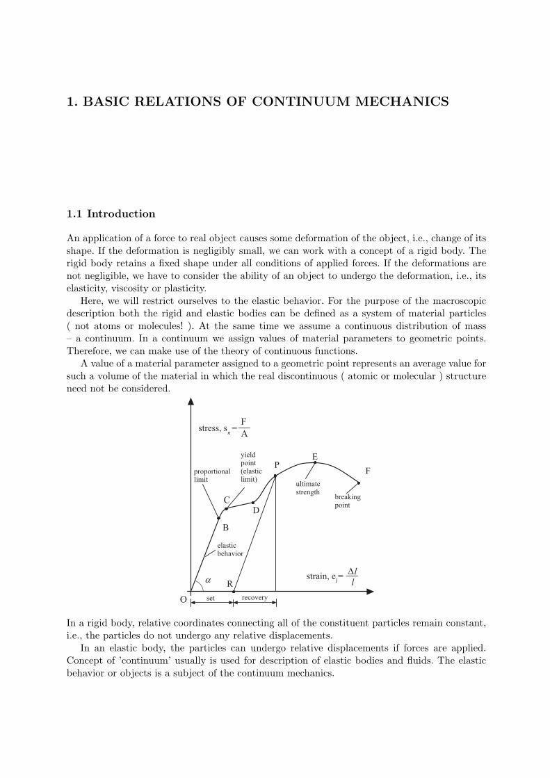
An application of a force to real object causes some deformation of the object, i.e., change of itsshape. If the deformation is negligibly small, we can work with a concept of a rigid body. Therigid body retains a fixed shape under all conditions of applied forces. If the deformations arenot negligible, we have to consider the ability of an object to undergo the deformation, i.e., itselasticity, viscosity or plasticity.
Here, we will restrict ourselves to the elastic behavior. For the purpose of the macroscopicdescription both the rigid and elastic bodies can be defined as a system of material particles( not atoms or molecules! ). At the same time we assume a continuous distribution of mass– a continuum. In a continuum we assign values of material parameters to geometric points.Therefore, we can make use of the theory of continuous functions.
A value of a material parameter assigned to a geometric point represents an average value forsuch a volume of the material in which the real discontinuous ( atomic or molecular ) structureneed not be considered.
In a rigid body, relative coordinates connecting all of the constituent particles remain constant,i.e., the particles do not undergo any relative displacements.
In an elastic body, the particles can undergo relative displacements if forces are applied.Concept of ’continuum’ usually is used for description of elastic bodies and fluids. The elasticbehavior or objects is a subject of the continuum mechanics.
2 1. BASIC RELATIONS
1.2 Body forces
Non-contact forces proportional to mass contained in a considered volume of a continuum.
- forces between particles that are not adjacent; e.g., mutual gravitational forces- forces due to the application of physical processes external to the considered volume; e.g.,
forces acting on buried particles of iron when a magnet is moving outside the consideredvolume
Let ~f(~x, t) be a body force acting per unit volume on the particle that was at position ~x at somereference time. An important case of a body force – a force applied impulsively to one particleat ~x = ~ξ and t = τ in the direction of the xn-axis
fi(~x, t) = Aδ(~x− ~ξ)δ(t− τ)δin (1.1)[fi]
U = Nm−3, [δ(~x− ~ξ)]U = m−3
[A]U = Ns, [δ(t− τ)]U = s−1
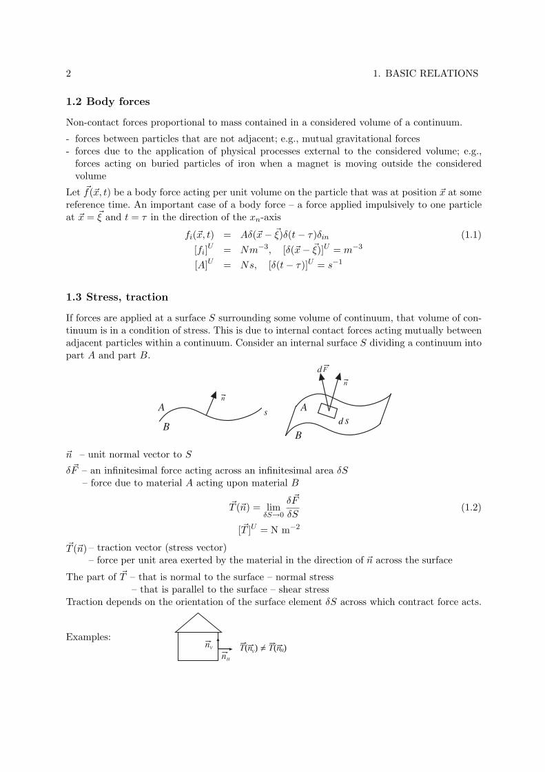
1.3 Stress, traction
If forces are applied at a surface S surrounding some volume of continuum, that volume of con-tinuum is in a condition of stress. This is due to internal contact forces acting mutually betweenadjacent particles within a continuum. Consider an internal surface S dividing a continuum intopart A and part B.
d
s
B
A
n
A
B
s
Fd
n
~n – unit normal vector to S
δ ~F – an infinitesimal force acting across an infinitesimal area δS– force due to material A acting upon material B
~T (~n) = limδS→0
δ ~F
δS(1.2)
[~T ]U = N m−2
~T (~n) – traction vector (stress vector)– force per unit area exerted by the material in the direction of ~n across the surface
The part of ~T – that is normal to the surface – normal stress– that is parallel to the surface – shear stress
Traction depends on the orientation of the surface element δS across which contract force acts.
Examples:V
nH
nV T(n ) = T(n )H
1.4 Displacement, strain 3
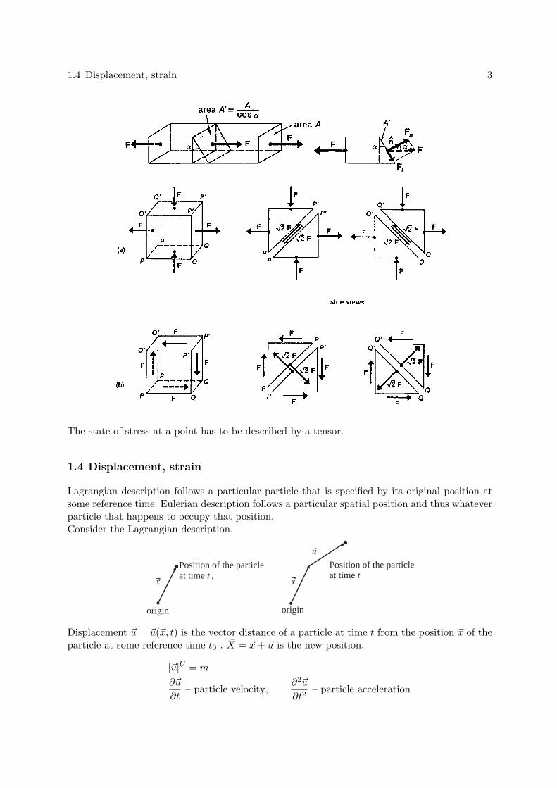
The state of stress at a point has to be described by a tensor.
1.4 Displacement, strain
Lagrangian description follows a particular particle that is specified by its original position atsome reference time. Eulerian description follows a particular spatial position and thus whateverparticle that happens to occupy that position.Consider the Lagrangian description.
Position of the particleat time t
origin
0
origin
u
xx
Position of the particleat time t
Displacement ~u = ~u(~x, t) is the vector distance of a particle at time t from the position ~x of theparticle at some reference time t0 . ~X = ~x + ~u is the new position.
[~u]U = m
∂~u
∂t– particle velocity,
∂2~u
∂t2– particle acceleration
4 1. BASIC RELATIONS
~u can generally include both the deformation and rigid–body translation and rotation. To analyzethe deformation, we compare displacements of two neighboring particles.
~D = ~u(~x + ~d)− ~u(~x) (1.3a)Di = ui(xj + dj)− ui(xj) (1.3b)
ui(xj + dj).= ui(xj) + ui,jdj (1.4a)(
ui,j =∂ui
∂xj
)
~u(~x + ~d) .= ~u(~x) + (~d · ∇)~u(~x) (1.4b)
~u(~x + ~d) = ~u(~x) +
u1,1 u1,2 u1,3
u2,1 u2,2 u2,3
u3,1 u3,2 u3,3
d1
d2
d3
(1.4c)
Di = ui,jdj (1.5)
ui,j =12(ui,j + uj,i) +
12(ui,j − uj,i) (1.6)
eij =12(ui,j + uj,i) symmetric tensor (1.7a)
Ωij =12(ui,j − uj,i) antisymmetric tensor (1.8a)
eij =
u1,112(u1,2 + u2,1) 1
2(u1,3 + u3,1)12(u2,1 + u1,2) u2,2
12(u2,3 + u3,2)
12(u3,1 + u1,3) 1
2(u3,2 + u2,3) u3,3
(1.7b)
Ωij =
0 12(u1,2 − u2,1) 1
2(u1,3 − u3,1)12(u2,1 − u1,2) 0 1
2(u2,3 − u3,2)12(u3,1 − u1,3) 1
2(u3,2 − u2,3) 0
(1.8b)
Di = eijdj + Ωijdj (1.9)
z
x
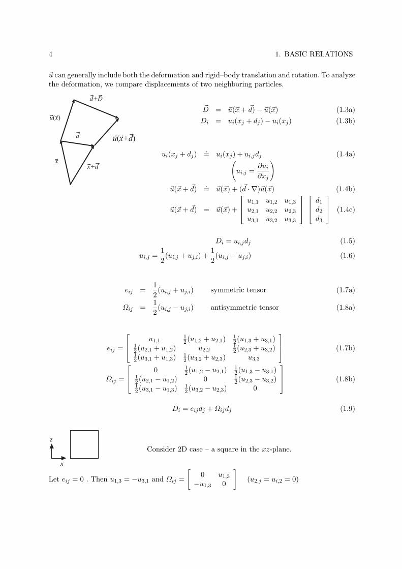
Consider 2D case – a square in the xz-plane.
Let eij = 0 . Then u1,3 = −u3,1 and Ωij =
[0 u1,3
−u1,3 0
](u2,j = ui,2 = 0)
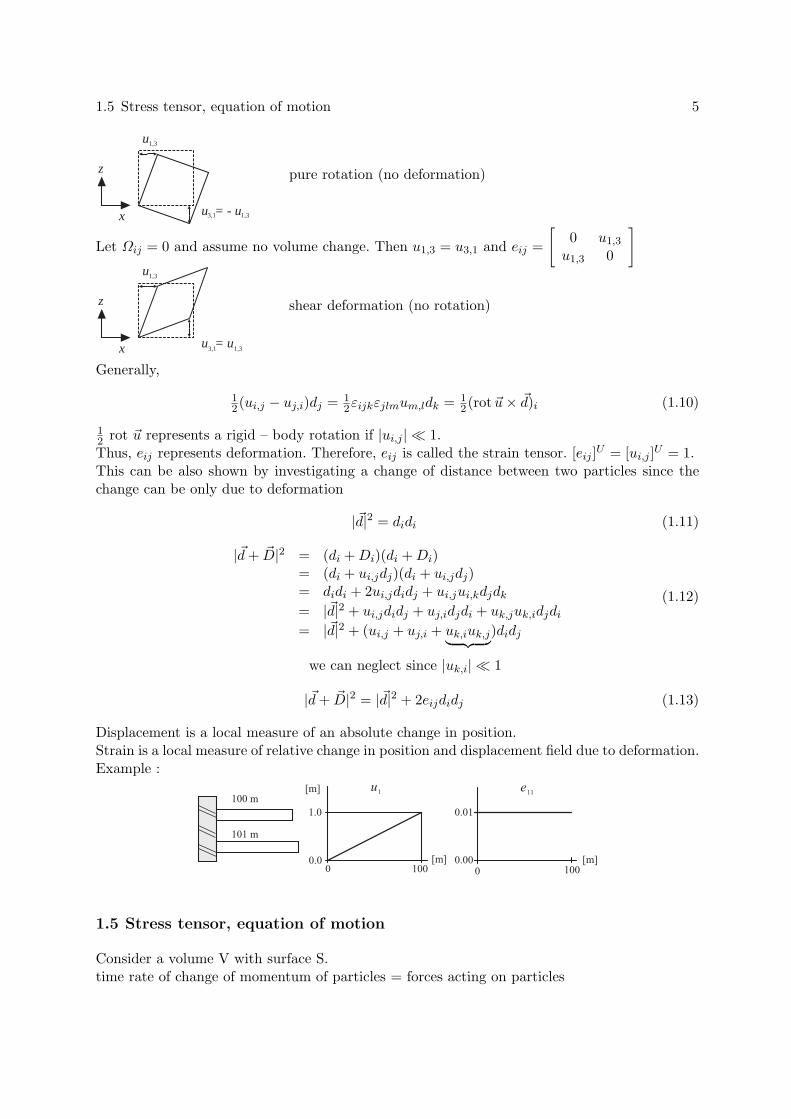
1.5 Stress tensor, equation of motion 5
u1,3
u = - u1,33,1
z
x
pure rotation (no deformation)
Let Ωij = 0 and assume no volume change. Then u1,3 = u3,1 and eij =
[0 u1,3
u1,3 0
]
u1,3
u = u1,33,1
z
x
shear deformation (no rotation)
Generally,
12(ui,j − uj,i)dj = 1
2εijkεjlmum,ldk = 12(rot ~u× ~d)i (1.10)
12 rot ~u represents a rigid – body rotation if |ui,j | ¿ 1.Thus, eij represents deformation. Therefore, eij is called the strain tensor. [eij ]U = [ui,j ]U = 1.This can be also shown by investigating a change of distance between two particles since thechange can be only due to deformation
|~d|2 = didi (1.11)
|~d + ~D|2 = (di + Di)(di + Di)= (di + ui,jdj)(di + ui,jdj)= didi + 2ui,jdidj + ui,jui,kdjdk
= |~d|2 + ui,jdidj + uj,idjdi + uk,juk,idjdi
= |~d|2 + (ui,j + uj,i + uk,iuk,j︸ ︷︷ ︸)didj
(1.12)
we can neglect since |uk,i| ¿ 1
|~d + ~D|2 = |~d|2 + 2eijdidj (1.13)
Displacement is a local measure of an absolute change in position.Strain is a local measure of relative change in position and displacement field due to deformation.Example :
1.5 Stress tensor, equation of motion
Consider a volume V with surface S.time rate of change of momentum of particles = forces acting on particles
6 1. BASIC RELATIONS
∂
∂t
∫∫
V
∫ρ∂~u
∂tdV =
∫∫
V
∫~f dV +
∫
S
∫~T (~n) dS (1.14)
Since V and S move with the particles (Lagrangian description), ρdV does not change with timeand
∂
∂t
∫∫
V
∫ρ∂~u
∂tdV =
∫∫
V
∫ρ∂2~u
∂t2dV (1.15)
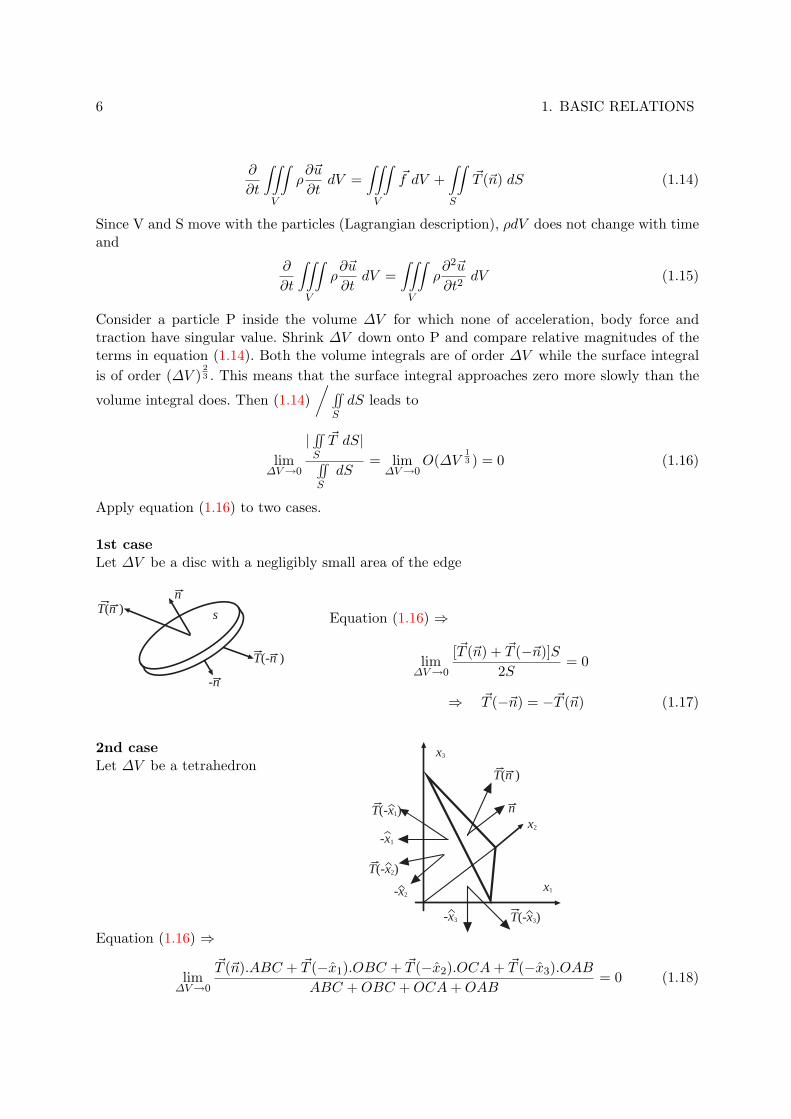
Consider a particle P inside the volume ∆V for which none of acceleration, body force andtraction have singular value. Shrink ∆V down onto P and compare relative magnitudes of theterms in equation (1.14). Both the volume integrals are of order ∆V while the surface integralis of order (∆V )
23 . This means that the surface integral approaches zero more slowly than the
volume integral does. Then (1.14)/ ∫
S
∫dS leads to
lim∆V→0
| ∫S
∫~T dS|
∫S
∫dS
= lim∆V→0
O(∆V13 ) = 0 (1.16)
Apply equation (1.16) to two cases.
1st caseLet ∆V be a disc with a negligibly small area of the edge
nT(n ) s
-n
T(-n )
Equation (1.16) ⇒
lim∆V→0
[~T (~n) + ~T (−~n)]S2S
= 0
⇒ ~T (−~n) = −~T (~n) (1.17)
2nd caseLet ∆V be a tetrahedron
x1
x2
x3
T(n )
nT(-x1)
T(-x2)
T(-x3)
-x1
-x2
-x3
Equation (1.16) ⇒
lim∆V→0
~T (~n).ABC + ~T (−x1).OBC + ~T (−x2).OCA + ~T (−x3).OAB
ABC + OBC + OCA + OAB= 0 (1.18)
1.5 Stress tensor, equation of motion 7
Since ~n = (n1, n2, n3);n1 = OBC/ABC , n2 = OCA/ABC , n3 = OAB/ABC (1.19)
and
~T (−xi) = −~T (xi); i = 1, 2, 3
we get from (1.18) after dividing it by ABC
lim∆V→0
~T (~n)− ~T (x1)n1 − ~T (x2)n2 − ~T (x3)n3
ABC + OBC + OCA + OAB= 0
and consequently
~T (~n) = ~T (xj)nj (1.20)Ti(~n) = Ti(xj)nj
Both properties (1.17) and (1.20) are important since they are valid in a dynamic case. (Theirvalidity in a static case is trivial.)Equation (1.20) can be written as
[T1(~n), T2(~n), T3(~n)] = [n1, n2, n3]
T1(x1) T2(x1) T3(x1)T1(x2) T2(x2) T3(x2)T1(x3) T2(x3) T3(x3)
(1.21)
Define stress tensor τji
τji = Ti(xj) (1.22)
[τji]U = Nm−2
Then (1.20) and (1.21) can be rewritten as
Ti(~n) = τjinj – Cauchy’s stress formula (1.23)
and
[T1(~n), T2(~n), T3(~n)] = [n1, n2, n3]
τ11 τ12 τ13
τ21 τ22 τ23
τ31 τ32 τ33
(1.24)
τji is the i-th component of the traction exerted by a material with greater xj across the planenormal to the j-th axis on material with lesser xj .

8 1. BASIC RELATIONS
Example:
Stress tensor fully describes a state of stress at a given point.Now we can apply eq. (1.23) to eq. (1.14). Eq. (1.14) in the index notation is
∫∫
V
∫ρui,tt dV =
∫∫
V
∫fi dV +
∫
S
∫Ti(~n) dS (1.25)
Using eq. (1.23) the surface integral becomes∫
S
∫τjinj dS =
∫
S
∫τji dSj (1.26)
The surface integral can be transformed into a volume integral using Gauss’s divergence theorem
∫
S
∫~a ~dS =
∫∫
V
∫div ~a dV
∫
S
∫aj dSj =
∫∫
V
∫∂aj
∂ξjdV (~ξ)
In our problem, the particles constituting S have moved from their original positions ~x at thereference time to position ~X = ~x + ~u at time t. Therefore, the spatial differentiation in volumeV is ∂
∂Xj. The application of Gauss’s theorem thus gives
∫
S
∫τji dSj =
∫∫
V
∫∂τji
∂XjdV (1.27)
Eq. (1.25) can be now written as
∫∫
V
∫(ρui,tt − fi − τji,j) dV = 0 (1.28)
where τji,j = ∂τji/∂Xj
The integrand in (1.28) must be zero everywhere where it is continuous. Therefore,
ρui,tt = τji,j + fi (1.29)
This is the equation of motion for the elastic continuum. Look now at the angular momentumof the particles in a volume V.
1.5 Stress tensor, equation of motion 9
time rate of change of angularmomentum about the origin
= moment of forces (torque)acting on the particles
∂
∂t
∫∫
V
∫~X × ρ~ut dV =
∫∫
V
∫~X × ~f dV +
∫
S
∫~X × ~T dS (1.30)
∂∂t( ~X × ~ut) = ~Xt × ~ut + ~X × ~utt = ( ~xt︸︷︷︸
=0
+ ~ut)× ~ut︸ ︷︷ ︸=0
+ ~X × ~utt = ~X × ~utt (1.31)
Then eq. (1.30) ⇒∫∫
V
∫εijkXj(ρuk,tt − fk)dV =
∫
S
∫εijkXjTk dS (1.32)
Eq. (1.29) implies∫∫
V
∫εijkXj
∂τlk
∂XldV =
∫∫
V
∫εijkXj(ρuk,tt − fk) dV (1.33)
The right-hand side of eq. (1.33) can be replaced by the right-hand side of eq. (1.32)
∫∫
V
∫εijkXj
∂τlk
∂XldV =
∫
S
∫εijkXjTk dS (1.34)
eq. (1.23) ⇒ =∫
S
∫εijkXjτlknl dS
Gauss’s theorem ⇒ =∫∫
V
∫εijk
∂
∂Xl(Xjτlk) dV
∂
∂Xl(Xjτlk) = δjlτlk + Xj
∂τlk
∂Xl= τjk + Xj
∂τlk
∂Xl
Then eq. (1.34) becomes
∫∫
V
∫εijkXj
∂τlk
∂XldV =
∫∫
V
∫ (εijkτjk + εijkXj
∂τlk
∂Xl
)dV
This gives∫∫
V
∫εijk τjk dV = 0 (1.35)
Since eq. (1.35) applies to any volume
εijk τjk = 0 (1.36)
and consequently
τjk = τkj (1.37)
10 1. BASIC RELATIONS
which means that the stress tensor is symmetric. This is a very important property meaningthat the stress tensor has only 6 independent components. The state of stress at a given pointis thus fully described by 6 independent components of the stress tensor.
We can now rewrite relation for traction (1.23) and equation of motion (1.29) as
Ti = τijnj (1.38)ρui,tt = τij,j + fi (1.39)
Strictly, τij,j = ∂τij
∂Xj. In the case of seismic wave propagation, displacement, strain, acceleration
and stress vary over distances much larger than the amplitude of particle displacement and theother quantities. Therefore, differentiation with respect to xj gives a very good approximationof differentiation with respect to Xj . In other words, the difference between derivative evaluatedfor a particular particle (∼ Lagrangian description) and derivative evaluated at a fixed position(∼ Eulerian description) is negligible.
1.6 Stress - strain relation. Strain - energy function.
The mechanical behavior of a continuum is defined by the relation between the stress and strain.If forces are applied to the continuum, the stress and strain change together according to thestress–strain relation. Such the relation is called the constitutive relation.A linear elastic continuum is described by Hooke’s law which in Cauchy’s generalized formulationreads
τij = cijklekl (1.40)
Each component of the stress tensor is a linear combination of all components of the straintensor. cijkl is the 4th – order tensor of elastic coefficients and has 34 = 81 components.
τij = τji ⇒ cijkl = cjikl (1.41)ekl = elk ⇒ cijkl = cijlk (1.42)
The symmetry of the stress and strain tensors reduces the number of different coefficients to6 × 6 = 36. A further reduction of the number of coefficients follows from the first law ofthermodynamics which will also give a formula for the strain-energy function.
Rate of mechanical work + Rate of heating= Rate of increase of kinetic and internal energies (1.43)
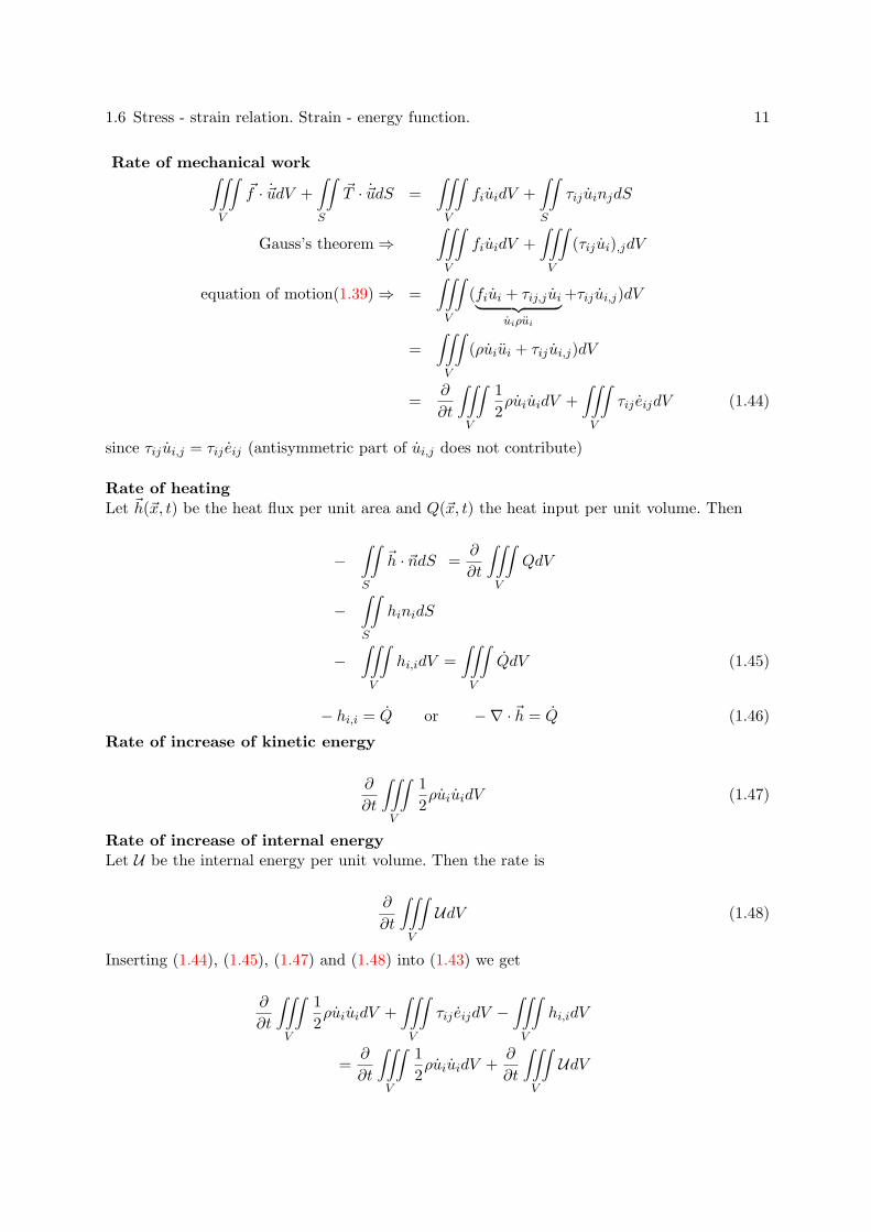
1.6 Stress - strain relation. Strain - energy function. 11
Rate of mechanical work∫∫
V
∫~f · ~udV +
∫
S
∫~T · ~udS =
∫∫
V
∫fiuidV +
∫
S
∫τij uinjdS
Gauss’s theorem ⇒∫∫
V
∫fiuidV +
∫∫
V
∫(τij ui),jdV
equation of motion(1.39) ⇒ =∫∫
V
∫(fiui + τij,j ui︸ ︷︷ ︸
uiρui
+τij ui,j)dV
=∫∫
V
∫(ρuiui + τij ui,j)dV
=∂
∂t
∫∫
V
∫ 12ρuiuidV +
∫∫
V
∫τij eijdV (1.44)
since τij ui,j = τij eij (antisymmetric part of ui,j does not contribute)
Rate of heatingLet ~h(~x, t) be the heat flux per unit area and Q(~x, t) the heat input per unit volume. Then
−∫
S
∫~h · ~ndS =
∂
∂t
∫∫
V
∫QdV
−∫
S
∫hinidS
−∫∫
V
∫hi,idV =
∫∫
V
∫QdV (1.45)
− hi,i = Q or −∇ · ~h = Q (1.46)
Rate of increase of kinetic energy
∂
∂t
∫∫
V
∫ 12ρuiuidV (1.47)
Rate of increase of internal energyLet U be the internal energy per unit volume. Then the rate is
∂
∂t
∫∫
V
∫UdV (1.48)
Inserting (1.44), (1.45), (1.47) and (1.48) into (1.43) we get
∂
∂t
∫∫
V
∫ 12ρuiuidV +
∫∫
V
∫τij eijdV −
∫∫
V
∫hi,idV
=∂
∂t
∫∫
V
∫ 12ρuiuidV +
∂
∂t
∫∫
V
∫UdV
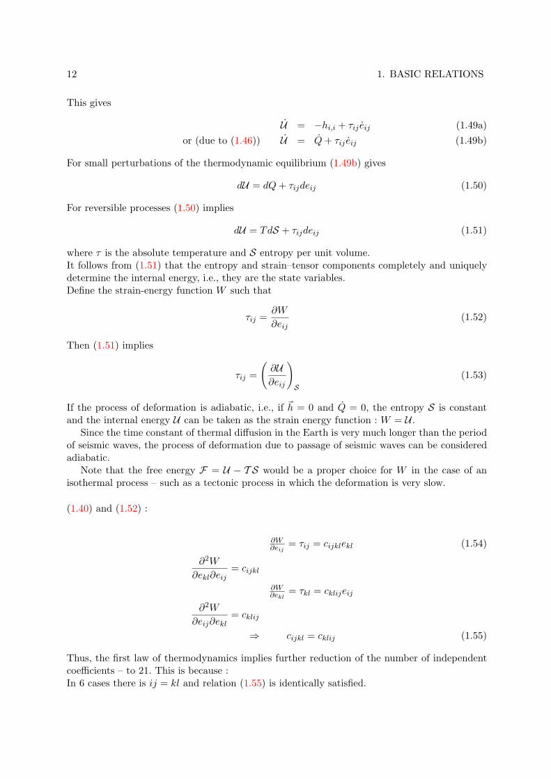
12 1. BASIC RELATIONS
This gives
U = −hi,i + τij eij (1.49a)or (due to (1.46)) U = Q + τij eij (1.49b)
For small perturbations of the thermodynamic equilibrium (1.49b) gives
dU = dQ + τijdeij (1.50)
For reversible processes (1.50) implies
dU = TdS + τijdeij (1.51)
where τ is the absolute temperature and S entropy per unit volume.It follows from (1.51) that the entropy and strain–tensor components completely and uniquelydetermine the internal energy, i.e., they are the state variables.Define the strain-energy function W such that
τij =∂W
∂eij(1.52)
Then (1.51) implies
τij =
(∂U∂eij
)
S(1.53)
If the process of deformation is adiabatic, i.e., if ~h = 0 and Q = 0, the entropy S is constantand the internal energy U can be taken as the strain energy function : W = U .
Since the time constant of thermal diffusion in the Earth is very much longer than the periodof seismic waves, the process of deformation due to passage of seismic waves can be consideredadiabatic.
Note that the free energy F = U − T S would be a proper choice for W in the case of anisothermal process – such as a tectonic process in which the deformation is very slow.
(1.40) and (1.52) :
∂W∂eij
= τij = cijklekl (1.54)
∂2W
∂ekl∂eij= cijkl
∂W∂ekl
= τkl = cklijeij
∂2W
∂eij∂ekl= cklij
⇒ cijkl = cklij (1.55)
Thus, the first law of thermodynamics implies further reduction of the number of independentcoefficients – to 21. This is because :In 6 cases there is ij = kl and relation (1.55) is identically satisfied.
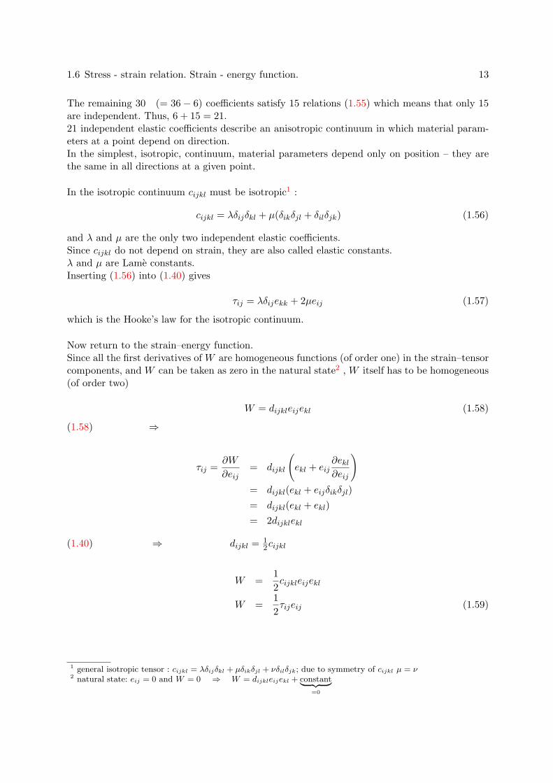
1.6 Stress - strain relation. Strain - energy function. 13
The remaining 30 (= 36− 6) coefficients satisfy 15 relations (1.55) which means that only 15are independent. Thus, 6 + 15 = 21.21 independent elastic coefficients describe an anisotropic continuum in which material param-eters at a point depend on direction.In the simplest, isotropic, continuum, material parameters depend only on position – they arethe same in all directions at a given point.
In the isotropic continuum cijkl must be isotropic1 :
cijkl = λδijδkl + µ(δikδjl + δilδjk) (1.56)
and λ and µ are the only two independent elastic coefficients.Since cijkl do not depend on strain, they are also called elastic constants.λ and µ are Lame constants.Inserting (1.56) into (1.40) gives
τij = λδijekk + 2µeij (1.57)
which is the Hooke’s law for the isotropic continuum.
Now return to the strain–energy function.Since all the first derivatives of W are homogeneous functions (of order one) in the strain–tensorcomponents, and W can be taken as zero in the natural state2 , W itself has to be homogeneous(of order two)
W = dijkleijekl (1.58)
(1.58) ⇒
τij =∂W
∂eij= dijkl
(ekl + eij
∂ekl
∂eij
)
= dijkl(ekl + eijδikδjl)= dijkl(ekl + ekl)= 2dijklekl
(1.40) ⇒ dijkl = 12cijkl
W =12cijkleijekl
W =12τijeij (1.59)
1 general isotropic tensor : cijkl = λδijδkl + µδikδjl + νδilδjk; due to symmetry of cijkl µ = ν2 natural state: eij = 0 and W = 0 ⇒ W = dijkleijekl + constant︸ ︷︷ ︸
=0
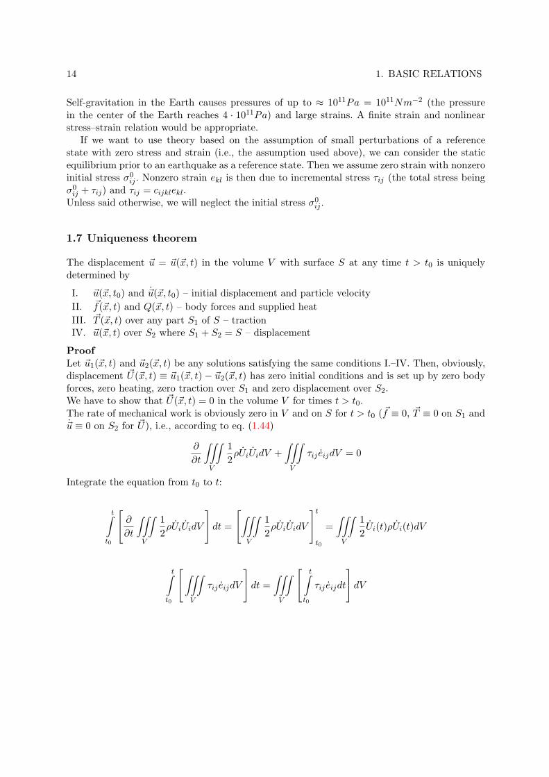
14 1. BASIC RELATIONS
Self-gravitation in the Earth causes pressures of up to ≈ 1011Pa = 1011Nm−2 (the pressurein the center of the Earth reaches 4 · 1011Pa) and large strains. A finite strain and nonlinearstress–strain relation would be appropriate.
If we want to use theory based on the assumption of small perturbations of a referencestate with zero stress and strain (i.e., the assumption used above), we can consider the staticequilibrium prior to an earthquake as a reference state. Then we assume zero strain with nonzeroinitial stress σ0
ij . Nonzero strain ekl is then due to incremental stress τij (the total stress beingσ0
ij + τij) and τij = cijklekl.Unless said otherwise, we will neglect the initial stress σ0
ij .
1.7 Uniqueness theorem
The displacement ~u = ~u(~x, t) in the volume V with surface S at any time t > t0 is uniquelydetermined by
I. ~u(~x, t0) and ~u(~x, t0) – initial displacement and particle velocityII. ~f(~x, t) and Q(~x, t) – body forces and supplied heatIII. ~T (~x, t) over any part S1 of S – tractionIV. ~u(~x, t) over S2 where S1 + S2 = S – displacement
ProofLet ~u1(~x, t) and ~u2(~x, t) be any solutions satisfying the same conditions I.–IV. Then, obviously,displacement ~U(~x, t) ≡ ~u1(~x, t)− ~u2(~x, t) has zero initial conditions and is set up by zero bodyforces, zero heating, zero traction over S1 and zero displacement over S2.We have to show that ~U(~x, t) = 0 in the volume V for times t > t0.The rate of mechanical work is obviously zero in V and on S for t > t0 (~f ≡ 0, ~T ≡ 0 on S1 and~u ≡ 0 on S2 for ~U), i.e., according to eq. (1.44)
∂
∂t
∫∫
V
∫ 12ρUiUidV +
∫∫
V
∫τij eijdV = 0
Integrate the equation from t0 to t:
t∫
t0
∂
∂t
∫∫
V
∫ 12ρUiUidV
dt =
∫∫
V
∫ 12ρUiUidV
t
t0
=∫∫
V
∫ 12Ui(t)ρUi(t)dV
t∫
t0
∫∫
V
∫τij eijdV
dt =
∫∫
V
∫
t∫
t0
τij eijdt
dV
1.7 Uniqueness theorem 15
t∫
t0
τij eijdt = [τijeij ]tt0
−t∫
t0
τijeijdt
= [cijklekleij ]tt0
−t∫
t0
cijklekleijdt /cijkl = cklij
−t∫
t0
cklij ekleijdt /i ↔ k, j ↔ l
−t∫
t0
cijkleijekldt
−t∫
t0
cijklekleijdt
−t∫
t0
τij eijdt
t∫
t0
τij eijdt = [cijklekleij ]tt0
−t∫
t0
τij eijdt
t∫
t0
τij eijdt =12
[cijklekleij ]tt0
=12
[cijklUk,lUi,j ]tt0
=12cijklUk,l(~x, t)Ui,j(~x, t)
The integrated equation gives
∫∫
V
∫ 12ρUiUidV +
∫∫
V
∫ 12cijklUk,lUi,jdV = 0
Since both the kinetic and strain energies are positive, Ui(~x, t) = 0 for t ≥ t0. Since Ui(~x, t0) = 0,~U(~x, t) = 0 in V for t > t0.
16 1. BASIC RELATIONS
1.8 Reciprocity theorem
Consider volume V with surface S.Let ~u = ~u(~x, t) be displacement due to body force ~f , boundary conditions on S, and initialconditions at t = 0.Let ~v = ~v(~x, t) be displacement due to body force ~g, boundary conditions on S, and initialconditions at t = 0. Both the boundary and initial conditions are in general different from thosefor ~u.Let ~T (~u, ~n) and ~T (~v, ~n) be tractions due to ~u and ~v, respectively, acting across surface with thenormal ~n.Then (Betti’s theorem)
∫∫
V
∫ (~f − ρ~u
)· ~vdV +
∫
S
∫~T (~u, ~n) · ~vdS
=∫∫
V
∫ (~g − ρ~v
)· ~udV +
∫
S
∫~T (~v, ~n) · ~udS (1.60)
Proof
∫∫
V
∫(fi − ρui) vidV
︸ ︷︷ ︸+
∫
S
∫Ti(~u, ~n)vidS =
−∫∫
V
∫τij,jvidV (Eq. of motion (1.39))
Eq. (1.38) ⇒
∫
S
∫Ti(~u, ~n)vidS =
∫
S
∫τijnjvidS
=∫∫
V
∫(τijvi),jdV
=∫∫
V
∫τij,jvidV +
∫∫
V
∫τijvi,jdV
=∫∫V
∫τijvi,jdV
=∫∫V
∫cijkleklvi,jdV
=∫∫V
∫cijkluk,lvi,jdV
1.8 Reciprocity theorem 17
Analogously, it can be shown that the right–hand side of eq. (1.60) is equal to
∫∫V
∫cijklui,jvk,ldV
=∫∫V
∫cklijui,jvk,ldV ← cijkl = cklij interchanging indices
=∫∫V
∫cijkluk,lvi,jdV
which is the same as the left–hand side of eq. (1.60)It is important that– the theorem does not involve the initial conditions,– ~u, ~u, ~T (~u, ~n) and ~f may relate to time t1, while ~v, ~v, ~T (~v, ~n) and ~g may relate to time t2 6= t1
Let t1 = t and t2 = τ − t.Integrate Betti’s theorem (1.60) from 0 to τ , integrate first the acceleration terms:
τ∫
0
ρ[~u(t) · ~v(τ − t)− ~u(t) · ~v(τ − t)
]dt
= ρ
τ∫
0
∂
∂t
[~u(t) · ~v(τ − t)− ~u(t) · ~v(τ − t)
]dt
= ρ[~u(τ) · ~v(0)− ~u(0) · ~v(τ) + ~u(τ) · ~v(0) + ~u(0) · ~v(τ)
](1.61)
After the integration, the acceleration terms depend only on the initial (t = 0) and final (t = τ)values.Let ~u = 0 and ~v = 0 for τ ≤ τ0. Consequently, also ~u = 0 and ~v = 0 for τ ≤ τ0.Then it follows from eq. (1.61) that
∞∫
−∞ρ
[~u(t) · ~v(τ − t)− ~u(t) · ~v(τ − t)
]dt = 0 (1.62)
Integrating Betti’s theorem (1.60) from −∞ to ∞ and applying eq. (1.62) we obtain
∞∫
−∞dt
∫∫
V
∫ [~u(~x, t) · ~g(~x, τ − t)− ~v(~x, τ − t) · ~f(~x, t)
]dV
=∞∫
−∞dt
∫
S
∫ [~v(~x, τ − t) · ~T (~u(~x, t), ~n)− ~u(~x, t) · ~T (~v(~x, τ − t), ~n)
]dS (1.63)
This is the important reciprocity theorem for displacements ~u and ~v with a quiescent past.
18 1. BASIC RELATIONS
1.9 Green’s function
Let the unit impulse force in the direction of the xn – axis be applied at point ~ξ and time τ (seedefinition (1.1)):
fi(~x, t) = Aδ(~x− ~ξ)δ(t− τ)δin
Then the equation of motion is
ρui = (cijkluk,l),j + Aδ(~x− ~ξ)δ(t− τ)δin
ρui
A=
(cijkl
(ukA
),l
),j
+ δ(~x− ~ξ)δ(t− τ)δin
Define Green’s function Gin(~x, t; ~ξ, τ):
Gin(~x, t; ~ξ, τ) =ui
A; [Gin]U =
m
Ns=
s
kg
Green’s function satisfies equation
ρGin = (cijklGkn,l),j + δ(~x− ~ξ)δ(t− τ)δin (1.64)
Let A = 1Ns. Then the value of Gin(~x, t; ~ξ, τ) is equal to the value of the i–th component of thedisplacement at (~x, t) due to the unit impulse force applied at (~ξ, τ) in the direction of axis xn.To specify Gin uniquely, we have to specify initial conditions and boundary conditions on S.
Initial conditions:
Gin(~x, t, ~ξ, τ) = 0 and Gin(~x, t, ~ξ, τ) = 0 for t ≤ τ, ~x 6= ~ξ
Boundary conditions on S:
Time independent b.c.⇒ The time origin can obviously be arbitrarily shifted. Then eq. (1.64) implies
Gin(~x, t; ~ξ, τ) = Gin(~x, t− τ ; ~ξ, 0) = Gin(~x,−τ ; ~ξ,−t) (1.65)
Homogeneous boundary conditions (either the displacement or the traction is zero at every pointof the surface)Recall the reciprocity theorem (1.63):
∞∫
−∞dt
∫∫
V
∫ [~u(~x, t) · ~g(~x, τ − t)− ~v(~x, τ − t) · ~f(~x, t)
]dV
=∞∫
−∞dt
∫
S
∫ [~v(~x, τ − t) · ~T (~u(~x, t), ~n)− ~u(~x, t) · ~T (~v(~x, τ − t), ~n)
]dS
1.9 Green’s function 19
Let ~f and ~g be unit impulse forces
fi(~x, t) = Aδ(~x− ~ξ1)δ(t− τ1)δim (1.66a)gi(~x, t) = Aδ(~x− ~ξ2)δ(t + τ2)δin A = 1 Ns (1.66b)
Then the displacements ~u due to ~f and ~v due to ~g are
ui(~x, t) = AGim(~x, t; ~ξ1, τ1) (1.67a)vi(~x, t) = AGin(~x, t; ~ξ2,−τ2) (1.67b)
Eq.(1.66b) ⇒ gi(~x, τ − t) = Aδ(~x− ~ξ2)δ(τ − t + τ2)δin (1.68)Eq. (1.67b) ⇒ vi(~x, τ − t) = AGin(~x, τ − t; ~ξ2,−τ2) (1.69)
Insert (1.66a), (1.67a), (1.68) and (1.69) into (1.63)
∞∫
−∞dt
∫∫
V
∫ [Gim(~x, t; ~ξ1, τ1)δ(~x− ~ξ2)δ(τ − t + τ2)δin
−Gin(~x, τ − t; ~ξ2,−τ2)δ(~x− ~ξ1)δ(t− τ1)δim
]dV = 0
(The integral over S in (1.63) is zero due to homogeneous boundary conditions.)
Gnm(~ξ2, τ + τ2; ~ξ1, τ1) − Gmn(~ξ1, τ − τ1; ~ξ2,−τ2) = 0Gnm(~ξ2, τ + τ2; ~ξ1, τ1) = Gmn(~ξ1, τ − τ1; ~ξ2,−τ2) (1.70)
Let τ1 = τ2 = 0. Then eq. (1.70) implies
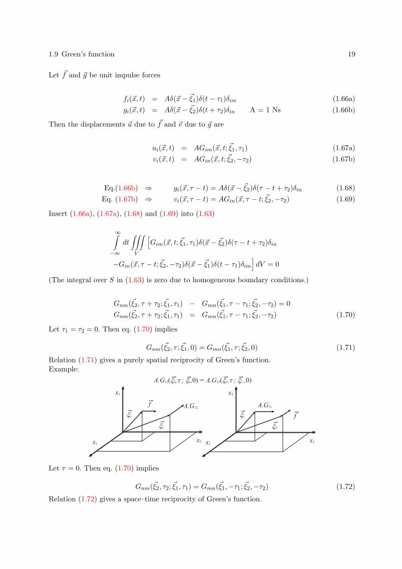
Gnm(~ξ2, τ ; ~ξ1, 0) = Gmn(~ξ1, τ ; ~ξ2, 0) (1.71)
Relation (1.71) gives a purely spatial reciprocity of Green’s function.Example:
Let τ = 0. Then eq. (1.70) implies
Gnm(~ξ2, τ2; ~ξ1, τ1) = Gmn(~ξ1,−τ1; ~ξ2,−τ2) (1.72)
Relation (1.72) gives a space–time reciprocity of Green’s function.
20 1. BASIC RELATIONS
1.10 Representation theorem
Find displacement ~u due to body forces ~f in volume V and to boundary conditions on surfaceS assuming
gi(~x, t) = Aδ(~x− ~ξ)δ(t)δin (1.73)
and corresponding displacement
vi(~x, t) = AGin(~x, t; ~ξ, 0) (1.74)
Insert (1.73) and (1.74) into the reciprocity theorem (1.63)
∞∫
−∞dt
∫∫
V
∫ [ui(~x, t)Aδ(~x− ~ξ)δ(τ − t)δin − AGin(~x, τ − t; ~ξ, 0)fi(~x, t)
]dV =
∞∫
−∞dt
∫
S
∫ [AGin(~x, τ − t; ~ξ, 0)Ti (~u(~x, t), ~n) − ui(~x, t)Ti
(AGkn(~x, τ − t; ~ξ, 0), ~n
)]dS(1.75)
Ti
(AGkn(~x, τ − t; ~ξ, 0), ~n
)= τijnj = cijklAGkn,l(~x, τ − t; ~ξ, 0)nj (1.76)
Inserting (1.76) into (1.75) we obtain
un(~ξ, τ) =∞∫
−∞dt
∫∫
V
∫fi(~x, t)Gin(~x, τ − t; ~ξ, 0)dV
+∞∫
−∞dt
∫
S
∫ [Gin(~x, τ − t; ~ξ, 0) Ti (~u(~x, t), ~n)
− ui(~x, t)cijklnj∂Gkn(~x, τ − t; ~ξ, 0)
∂ξl
]dS
Interchanging formally ~x and ~ξ as well as t and τ we have
~un(~x, t) =∞∫
−∞dτ
∫∫
V
∫fi(~ξ, τ)Gin(~ξ, t− τ ; ~x, 0)dV (~ξ)
+∞∫
−∞dτ
∫
S
∫ [Gin(~ξ, t− τ ; ~x, 0)Ti
(~u(~ξ, τ), ~n
)
− ui(~ξ, τ)cijkl(~ξ)njGkn,l(~ξ, t− τ ; ~x, 0)]dS(~ξ) (1.77)
Relation (1.77) gives displacement ~u at a point ~x and time t in terms of contributions due tobody force ~f in V , to traction ~T on S and to the displacement ~u itself on S. A disadvantage of
1.10 Representation theorem 21
the representation (1.77) is that the involved Green’s function corresponds to the impulse sourceat ~x and observation point at ~ξ.The reciprocity relations for Green’s function can be used to replace Green’s function in (1.77)by that corresponding to a source at ~ξ and observation point at ~x.Let S be a rigid boundary, i.e., a boundary with zero displacement:
Grigidin (~ξ, t− τ ; ~x, 0) = 0 for ~ξ in S.
The above condition is a homogeneous condition. Therefore, the spatial reciprocity relation(1.71) can be applied:
Grigidin (~ξ, t− τ ; ~x, 0) = Grigid
ni (~x, t− τ ; ~ξ, 0)
Inserting this into representation relation (1.77) we get
un(~x, t) =∞∫
−∞dτ
∫∫
V
∫fi(~ξ, τ)Grigid
ni (~x, t− τ ; ~ξ, 0)dV (~ξ)
−∞∫
−∞dτ
∫
S
∫ui(~ξ, τ)cijkl(~ξ)nj
∂Grigidnk
∂ξl(~x, t− τ ; ~ξ, 0)dS(~ξ) (1.78)
Let S be a free surface, i.e., a surface with zero traction:
cijklnj∂Gfree
kn (~ξ, t− τ ; ~x, 0)∂ξl
= 0 for ~ξ in S.
This is again a homogeneous condition and relation (1.71) can be applied. It follows from (1.77)that
un(~x, t) =∞∫
−∞dτ
∫∫
V
∫fi(~ξ, τ)Gfree
ni (~x, t− τ ; ~ξ, 0)dV (~ξ)
+∞∫
−∞dτ
∫
S
∫Gfree
ni (~x, t− τ ; ~ξ, 0) Ti
(~u(~ξ, τ), ~n
)dS(~ξ) (1.79)
References / Recommended Reading
Aki, K., Richards, P. G.: Quantitative Seismology: Theory and methods. W. H. Freeman 1980;University Science Books 2002
Barber, J. R.: Elasticity. Kluwer 2002Brdicka, M., Samek, L., Sopko, B.: Mechanika kontinua. Academia 2000Mase, G. T., Mase, G. E.: Continuum Mechanics for Engineers. CRC Press 1999Pujol, J.: Elastic Wave Propagation and Generation in Seismology. Cambridge University Press
2003