Basic Theorems and Concepts - Naval Postgraduate Schoolfaculty.nps.edu/jenn/EC4630/TheoremsandConceptsV2.pdf · Naval Postgraduate School Department of Electrical & Computer Engineering

AY2010 1

Basic Theorems and Concepts (Chapter 2)

EC4630 Radar and Laser Cross Section

Fall AY2011 Prof. D. Jenn [email protected]

AY2010 2

Naval Postgraduate School Department of Electrical & Computer Engineering Monterey, California

Introduction

Review/introduce basic concepts and tools for use in RCS analysis. Many are familiar from antenna analysis: Theorems:

• Uniqueness • Reciprocity • Duality • Superposition • Similitude

Principles:

• Method of images and boundary conditions

• Equivalence o Surface o Volume

• Magnetic currents • Equivalent currents • Huygen’s

Tools: • Radiation integrals (Stratton-Chu

integrals) • Far-field approximations • Physical optics approximation • Arrays of scatterers • Null field hypothesis • Surface impedance • Impedance boundary conditions • Discontinuity boundary conditions • Surface waves

AY2010 3


Review and Notation* (1)

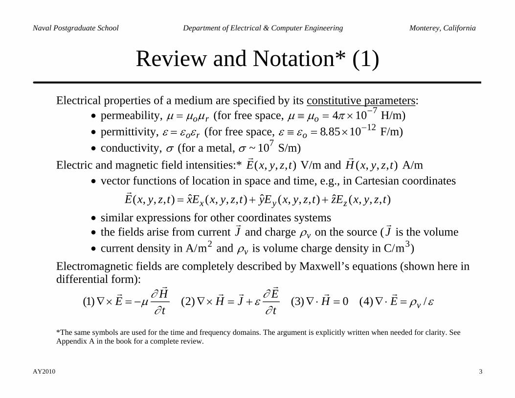
Electrical properties of a medium are specified by its constitutive parameters: • permeability, µ = µoµr (for free space, µ ≡ µo = 4π ×10−7 H/m) • permittivity, ε = εoεr (for free space, ε ≡ εo = 8.85 ×10−12 F/m) • conductivity, σ (for a metal, σ ~ 107 S/m)

Electric and magnetic field intensities:* ( , , , )E x y z t V/m and ( , , , )H x y z t A/m

• vector functions of location in space and time, e.g., in Cartesian coordinates

ˆ ˆ ˆ( , , , ) ( , , , ) ( , , , ) ( , , , )x y zE x y z t xE x y z t yE x y z t zE x y z t= + + • similar expressions for other coordinates systems • the fields arise from current

J and charge ρv on the source (

J is the volume

• current density in A/m2 and ρv is volume charge density in C/m3)

Electromagnetic fields are completely described by Maxwell’s equations (shown here in differential form):

(1) (2) (3) 0 (4) /vH EE H J H Et t

∂ ∂µ ε ρ ε∂ ∂

∇× = − ∇× = + ∇ ⋅ = ∇ ⋅ =

*The same symbols are used for the time and frequency domains. The argument is explicitly written when needed for clarity. See Appendix A in the book for a complete review.

AY2010 4


Review and Notation (2)

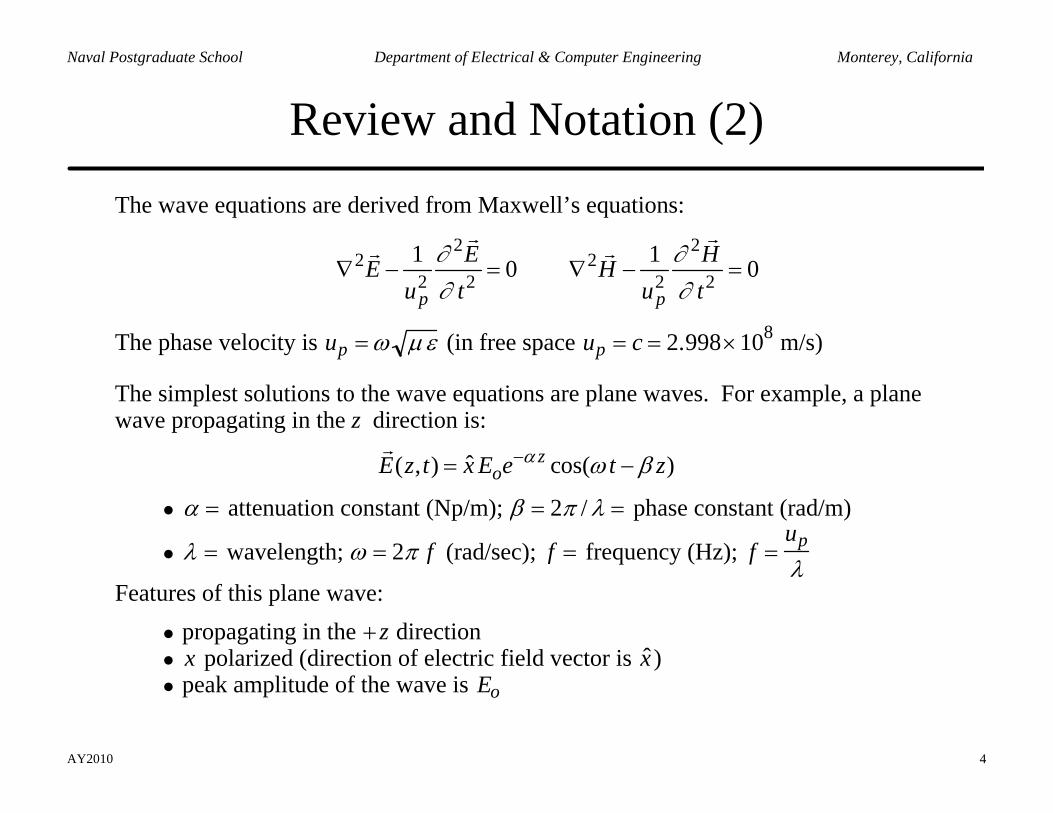
The wave equations are derived from Maxwell’s equations:

2 2

2 22 2 2 2

1 10 0p p

E HE Hu t u t

∂ ∂∂ ∂

∇ − = ∇ − =

The phase velocity is up = ω µ ε (in free space up = c = 2.998×108 m/s) The simplest solutions to the wave equations are plane waves. For example, a plane

wave propagating in the z direction is:

ˆ( , ) cos( )zoE z t x E e t zα ω β−= −

• α = attenuation constant (Np/m); β = 2π / λ = phase constant (rad/m)

• λ = wavelength; ω = 2π f (rad/sec); f = frequency (Hz); f =up

λ

Features of this plane wave:

• propagating in the + z direction • x polarized (direction of electric field vector is ˆ x ) • peak amplitude of the wave is Eo

AY2010 5



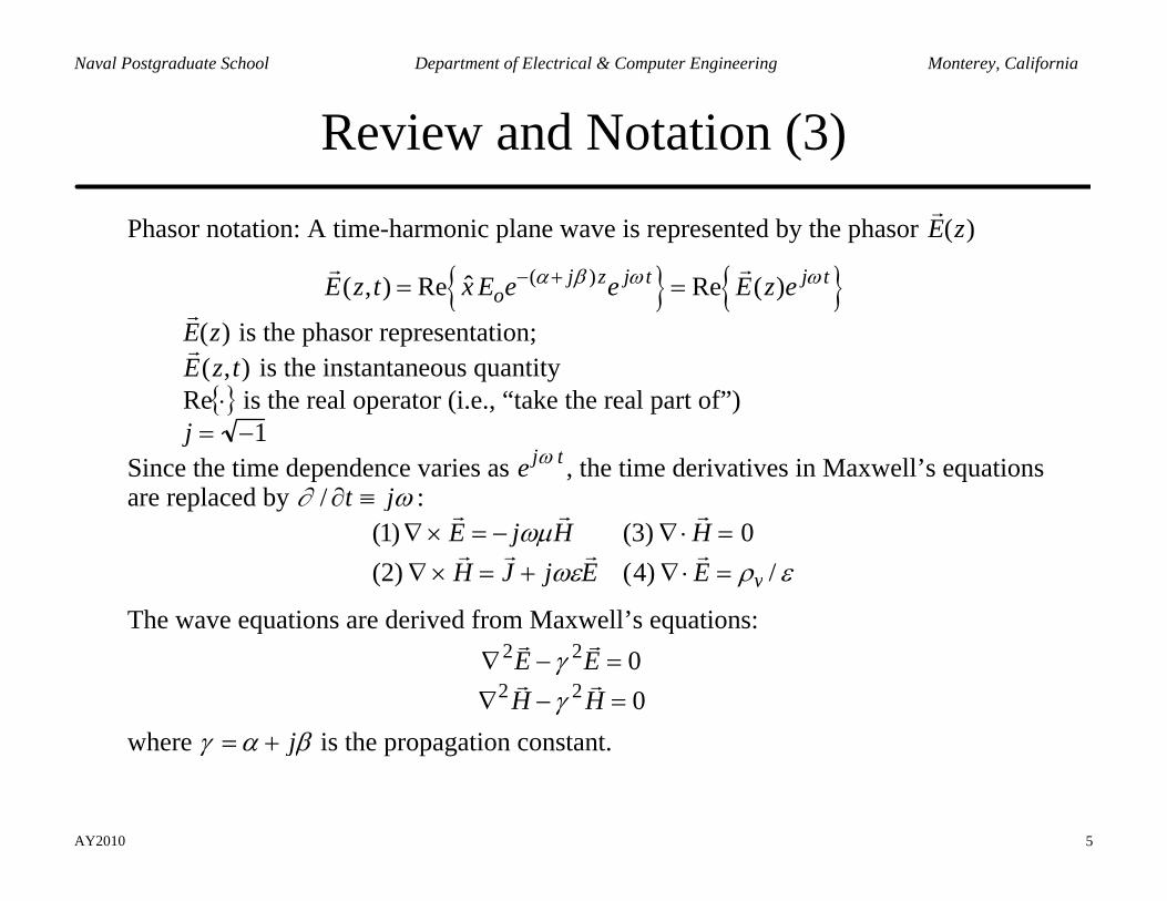
Phasor notation: A time-harmonic plane wave is represented by the phasor

E (z)

( )ˆ( , ) Re Re ( )j z j t j toE z t x E e e E z eα β ω ω− += =

E (z) is the phasor representation; ( , )E z t is the instantaneous quantity

⋅Re is the real operator (i.e., “take the real part of”) j = −1

Since the time dependence varies as e jω t , the time derivatives in Maxwell’s equations are replaced by ω∂ jt ≡∂/ :

(1) ∇ ×

E = − jωµ

H (3) ∇⋅

H = 0(2) ∇ ×

H =

J + jωε

E (4) ∇⋅

E = ρv / ε

The wave equations are derived from Maxwell’s equations:

∇2 E −γ 2

E = 0∇2

H −γ 2 H = 0

where γ = α + jβ is the propagation constant.

AY2010 6



Plane and spherical waves belong to a class called transverse electromagnetic (TEM). They have the following features:

1.

E ,

H and the direction of propagation ˆ k are mutually orthogonal 2.

E and

H are related by the intrinsic impedance of the medium

η =µ

(ε − jσ /ω )⇒ ηo =

µoεo

≈ 377 Ω for free space

The above relationships are expressed in the vector equation

H =

ˆ k ×

E η

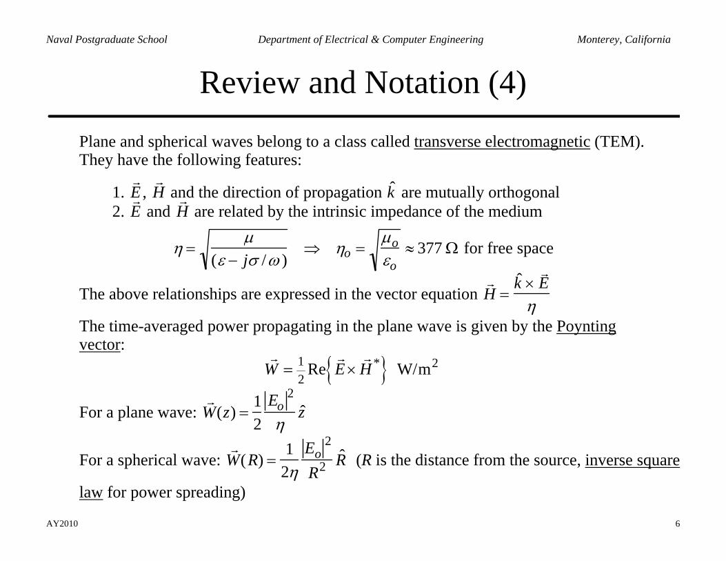
The time-averaged power propagating in the plane wave is given by the Poynting vector:

1 *2

ReW E H= × W/m2

For a plane wave:

W (z) =

12

Eo2

ηˆ z

For a spherical wave:

W (R) =

12η

Eo2

R2ˆ R (R is the distance from the source, inverse square

law for power spreading)

AY2010 7



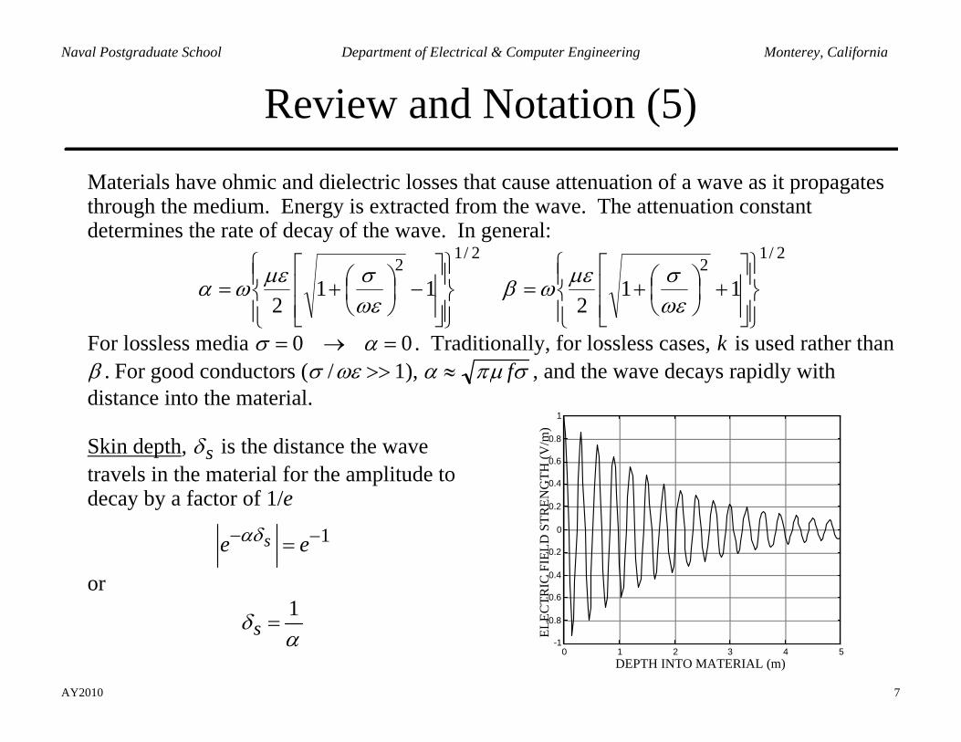
Materials have ohmic and dielectric losses that cause attenuation of a wave as it propagates through the medium. Energy is extracted from the wave. The attenuation constant determines the rate of decay of the wave. In general:

2/12

2/12

112

112 ⎪⎭

⎪⎬⎫

⎪⎩

⎪⎨⎧

⎥⎥⎦

⎤

⎢⎢⎣

⎡+⎟

⎠⎞

⎜⎝⎛+=

⎪⎭

⎪⎬⎫

⎪⎩

⎪⎨⎧

⎥⎥⎦

⎤

⎢⎢⎣

⎡−⎟

⎠⎞

⎜⎝⎛+=

ωεσµεωβ

ωεσµεωα

For lossless media 0 0σ α= → = . Traditionally, for lossless cases, k is used rather than β . For good conductors (σ /ωε >> 1), α ≈ πµ fσ , and the wave decays rapidly with distance into the material. Skin depth, sδ is the distance the wave travels in the material for the amplitude to decay by a factor of 1/e

1se eαδ− −=

or 1

sδα

= ELEC

TRIC

FIE

LD S

TREN

GTH

(V/m

)

DEPTH INTO MATERIAL (m)0 1 2 3 4 5

-1

-0.8

-0.6

-0.4

-0.2

0

0.2

0.4

0.6

0.8

1

AY2010 8



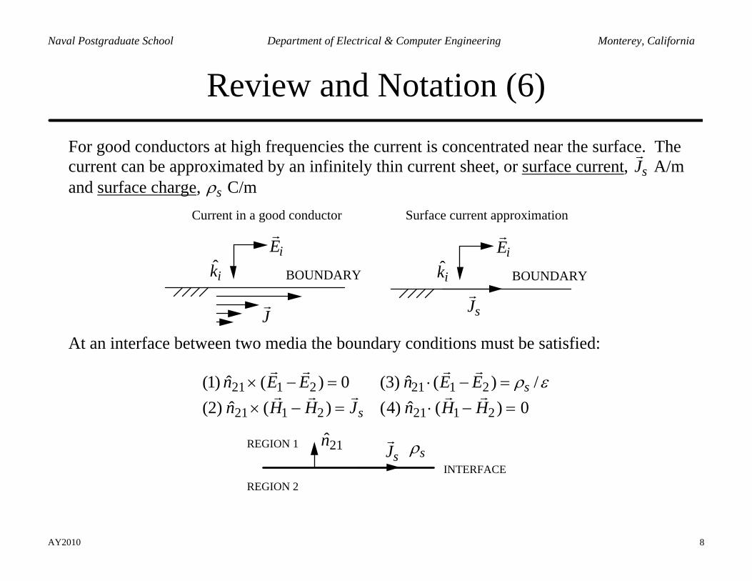
For good conductors at high frequencies the current is concentrated near the surface. The current can be approximated by an infinitely thin current sheet, or surface current,

J s A/m

and surface charge, ρs C/m

E iˆ k i

J

BOUNDARY

E i

ˆ k i BOUNDARY

J s

Current in a good conductor Surface current approximation

At an interface between two media the boundary conditions must be satisfied:

(1) ˆ n 21 × (

E 1 −

E 2 ) = 0 (3) ˆ n 21 ⋅(

E 1 −

E 2 ) = ρs /ε(2) ˆ n 21 × (

H 1 −

H 2 ) =

J s (4) ˆ n 21 ⋅ (

H 1 −

H 2 ) = 0

REGION 2

REGION 1

J s

ˆ n 21

INTERFACE

ρs

AY2010 9


Magnetic Current

To our knowledge, free magnetic charges do not exist. For convenience, fictitious magnetic charge and current are frequently included in Maxwell’s equations.

mJ = volume magnetic current density (V/m2)

msJ = surface magnetic current density (V/m) mvρ = volume magnetic charge density (C/m3) msρ = surface magnetic charge density (C/m2)

Time-harmonic form of Maxwell’s equations with magnetic charge and current:

(1) (3)(2) (4) /

m mv

v

E j H J BH J j E E

ωµ ρωε ρ ε

∇× = − − ∇ ⋅ =∇× = + ∇ ⋅ =

Boundary conditions at interfaces with magnetic surface charge and current:

21 1 2 21 1 2

21 1 2 21 1 2

ˆ ˆ(1) ( ) (3) ( )ˆ ˆ(2) ( ) (4) ( )

ms s

s ms

n E E J n D Dn H H J n B B

ρρ

× − = − ⋅ − =× − = ⋅ − =

AY2010 10


Basic Theorems Summarized

Uniqueness Theorem: For a given problem, a solution to Maxwell’s equations that satisfies the boundary conditions is unique. • This theorem allows us to construct equivalent problems to the original one that are

more easily solved. The equivalent problems are generally valid under some limited conditions (e.g. a limited region of space).

• An important fact arising from the uniqueness theorem is that a harmonic field ( , )E H in a source free dissipative region V is determined uniquely by the tangential components of E or H on the closed surface S that bounds the volume V.

Reciprocity Theorem: In general, the response of a system to a source is unchanged if the source and observer are interchanged. • As applied to antennas constructed of linear isotropic materials and reciprocal devices,

the transmitting and receiving patterns are identical.

Superposition Theorem: For a linear medium, Maxwell’s equations are linear. The total fields due to multiple sources turned on simultaneously is equal to the sum of the fields when energized separately. • Superposition applies to the complex vector electric and magnetic field intensities

( , )E H , not to the magnitudes ( , )E H or power 2 2(~ ,~ )E H !

AY2010 11


Basic Theorems Summarized

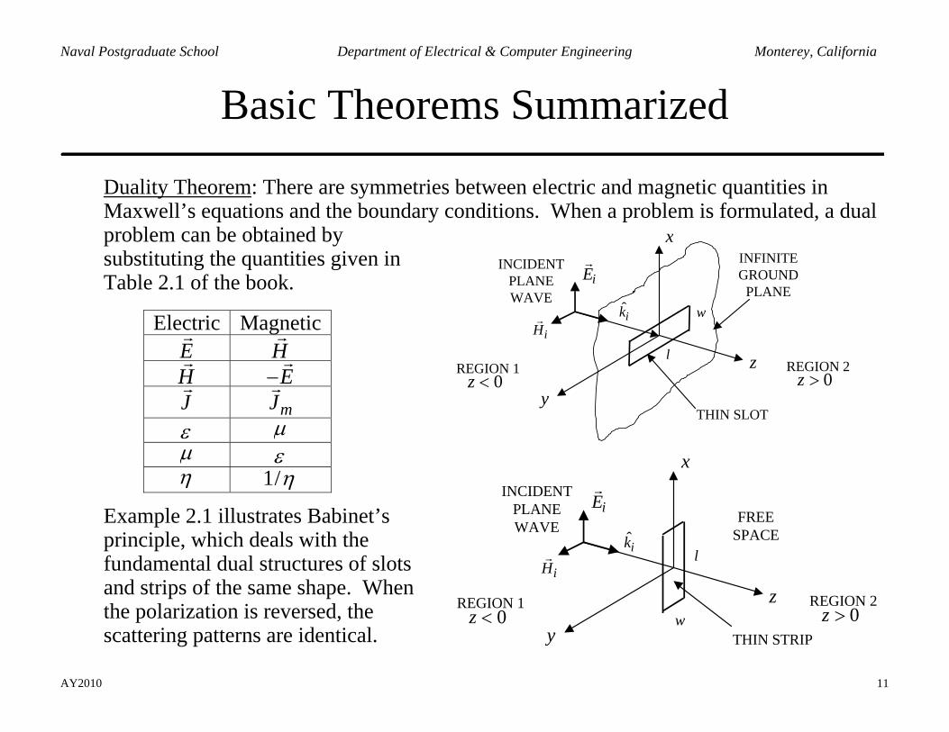
Duality Theorem: There are symmetries between electric and magnetic quantities in Maxwell’s equations and the boundary conditions. When a problem is formulated, a dual problem can be obtained by substituting the quantities given in Table 2.1 of the book.

Electric MagneticE H H E− J mJ ε µ µ ε η 1/η

Example 2.1 illustrates Babinet’s principle, which deals with the fundamental dual structures of slots and strips of the same shape. When the polarization is reversed, the scattering patterns are identical.

x

y

zREGION 1z < 0

REGION 2z > 0

E iINFINITEGROUND

PLANE

THIN SLOT

INCIDENTPLANEWAVE

ikiH

w

l

x

y

zREGION 1z < 0

REGION 2z > 0

FREESPACE

THIN STRIP

INCIDENTPLANEWAVE

ik

iH

w

l

E i

AY2010 12


Theorem of Similitude

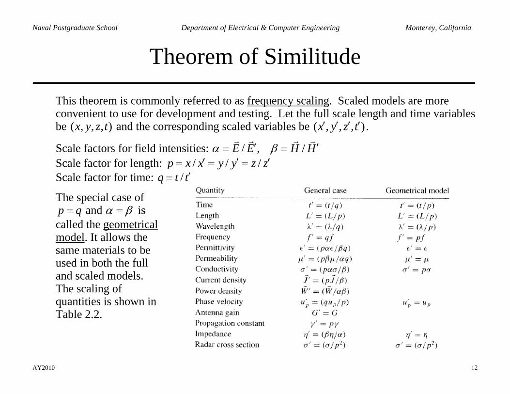
This theorem is commonly referred to as frequency scaling. Scaled models are more convenient to use for development and testing. Let the full scale length and time variables be ( , , , )x y z t and the corresponding scaled variables be ( , , , )x y z t′ ′ ′ ′ .

Scale factors for field intensities: / , /E E H Hα β′ ′= = Scale factor for length: / / /p x x y y z z′ ′ ′= = = Scale factor for time: /q t t′=

The special case of p q= and α β= is called the geometrical model. It allows the same materials to be used in both the full and scaled models. The scaling of quantities is shown in Table 2.2.

AY2010 13


Method of Images

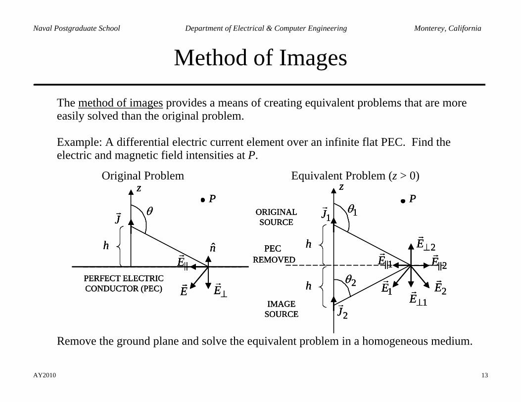
The method of images provides a means of creating equivalent problems that are more easily solved than the original problem.

Example: A differential electric current element over an infinite flat PEC. Find the electric and magnetic field intensities at P.

Original Problem Equivalent Problem (z > 0)

n

J

E

E⊥E

θ

z

h

PERFECT ELECTRICCONDUCTOR (PEC)

P

REMOVED

1J

1E

1E⊥1E

1θ

z

h

2E

2E⊥

2E

h

2J

2θ

ORIGINALSOURCE

IMAGESOURCE

P

PECn

J

E

E⊥E

θ

z

h


P

n

J

E

E⊥E

θ

z

h


P

REMOVED

1J

1E

1E⊥1E

1θ

z

h

2E

2E⊥

2E

h

2J

2θ

ORIGINALSOURCE

IMAGESOURCE

P

PECREMOVED

1J

1E

1E⊥1E

1θ

z

h

2E

2E⊥

2E

h

2J

2θ

ORIGINALSOURCE

IMAGESOURCE

P

PEC

Remove the ground plane and solve the equivalent problem in a homogeneous medium.

AY2010 14


Image Currents

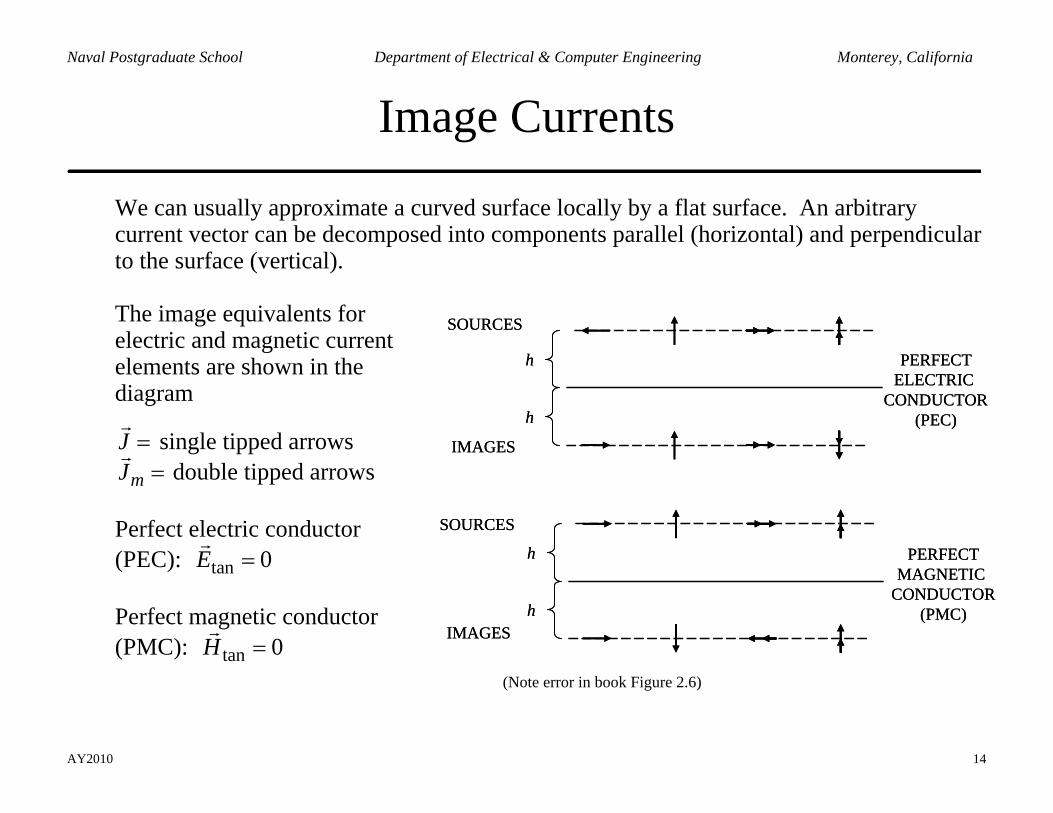
We can usually approximate a curved surface locally by a flat surface. An arbitrary current vector can be decomposed into components parallel (horizontal) and perpendicular to the surface (vertical).

The image equivalents for electric and magnetic current elements are shown in the diagram

J = single tipped arrows mJ = double tipped arrows

Perfect electric conductor (PEC): tan 0E = Perfect magnetic conductor (PMC): tan 0H =

SOURCES

IMAGES

PERFECTELECTRIC

CONDUCTOR(PEC)

h

h

PERFECTMAGNETIC

CONDUCTOR(PMC)

SOURCES

IMAGES

h

h

SOURCES

IMAGES

PERFECTELECTRIC

CONDUCTOR(PEC)

h

h

PERFECTMAGNETIC

CONDUCTOR(PMC)

SOURCES

IMAGES

h

h

(Note error in book Figure 2.6)

AY2010 15


Equivalence Principles

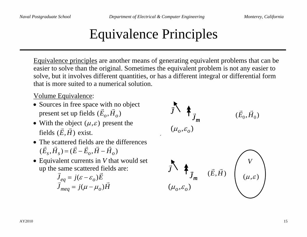
Equivalence principles are another means of generating equivalent problems that can be easier to solve than the original. Sometimes the equivalent problem is not any easier to solve, but it involves different quantities, or has a different integral or differential form that is more suited to a numerical solution.

Volume Equivalence: • Sources in free space with no object

present set up fields ( , )o oE H • With the object ( , )µ ε present the

fields ( , )E H exist. • The scattered fields are the differences

( , ) ( , )s s o oE H E E H H= − − • Equivalent currents in V that would set

up the same scattered fields are: ( )

( )eq o

meq o

J j EJ j H

ε εµ µ

= −= −

JmJ

, EVERYWHEµ ε ( , )o oµ ε

JmJ


0 0( , )E H

( , )µ ε

V

( , )E HJmJ

EVERYWHEε ( , )o oµ ε

JmJ


JmJ


JmJ


0 0( , )E H

( , )µ ε

V

( , )E HJmJ


JmJ


AY2010 16


Equivalence Principles

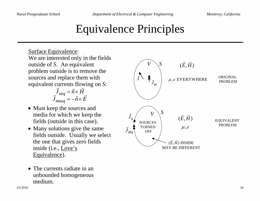
Surface Equivalence: We are interested only in the fields outside of S. An equivalent problem outside is to remove the sources and replace them with equivalent currents flowing on S:

ˆˆ

seqmseq

J n HJ n E

= ×= − ×

• Must keep the sources and media for which we keep the fields (outside in this case).

• Many solutions give the same fields outside. Usually we select the one that gives zero fields inside (i.e., Love’s Equivalence).

• The currents radiate in an

unbounded homogeneous medium.

JmJ

, EVERYWHEREµ ε

( , )E HSV

ORIGINAL PROBLEM

( , )E HSV

,µ ε

sJ

msJ

( , ) INSIDEMAY BE DIFFERENT

E H

EQUIVALENT PROBLEM

SOURCES TURNED

OFF

AY2010 17


Huygen’s Principle

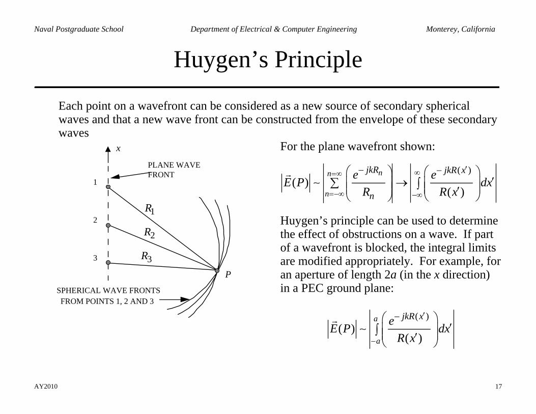
Each point on a wavefront can be considered as a new source of secondary spherical waves and that a new wave front can be constructed from the envelope of these secondary waves

PLANE WAVEFRONT

P

1

2

3

SPHERICAL WAVE FRONTS FROM POINTS 1, 2 AND 3

1R

2R

3R

x

For the plane wavefront shown:

( )( )

( )

nn

n

jkR jkR x

n

e eE P dxR R x

∞=∞

=−∞ −∞

′− −⎛ ⎞ ⎛ ⎞′→∑ ⎜ ⎟ ⎜ ⎟∫ ⎜ ⎟⎜ ⎟ ′⎝ ⎠⎝ ⎠

∼

Huygen’s principle can be used to determine the effect of obstructions on a wave. If part of a wavefront is blocked, the integral limits are modified appropriately. For example, for an aperture of length 2a (in the x direction) in a PEC ground plane:

( )( )

( )

a

a

jkR xeE P dxR x−

′−⎛ ⎞′⎜ ⎟∫ ⎜ ⎟′⎝ ⎠

∼

AY2010 18


Knife Edge Diffraction

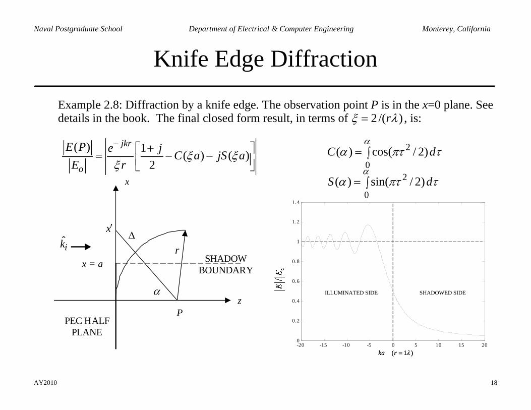
Example 2.8: Diffraction by a knife edge. The observation point P is in the x=0 plane. See details in the book. The final closed form result, in terms of 2 /( )rξ λ= , is:

( ) 1 ( ) ( )2

jkr

o

E P e j C a jS aE r

ξ ξξ

− +⎡ ⎤= − −⎢ ⎥⎣ ⎦

r

x

z

∆ik

x = a

P

α

x′

SHADOWBOUNDARY

PEC HALFPLANE

2

02

0

( ) cos( / 2)

( ) sin( / 2)

C d

S d

α

α

α πτ τ

α πτ τ

= ∫

= ∫

-20 -15 -10 -5 0 5 10 15 200

0.2

0.4

0.6

0.8

1

1.2

1.4

( 1 )ka r λ=

ILLUMINATED SIDE SHADOWED SIDE

-20 -15 -10 -5 0 5 10 15 200

0.2

0.4

0.6

0.8

1

1.2

1.4

( 1 )ka r λ=

ILLUMINATED SIDE SHADOWED SIDE

AY2010 19


Radiation Integrals

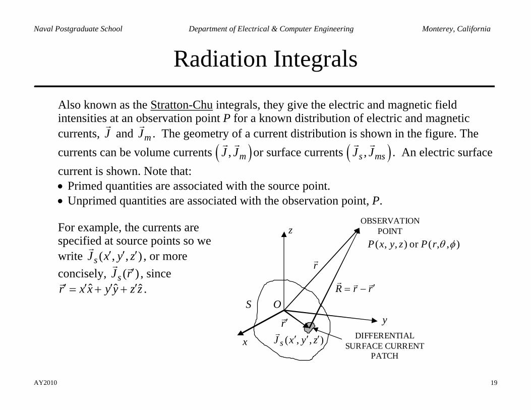
Also known as the Stratton-Chu integrals, they give the electric and magnetic field intensities at an observation point P for a known distribution of electric and magnetic currents, J and mJ . The geometry of a current distribution is shown in the figure. The currents can be volume currents ( ), mJ J or surface currents ( ),s msJ J . An electric surface current is shown. Note that: • Primed quantities are associated with the source point. • Unprimed quantities are associated with the observation point, P.

For example, the currents are specified at source points so we write ( , , )sJ x y z′ ′ ′ , or more concisely, ( )sJ r′ , since

ˆ ˆ ˆr x x y y z z′ ′ ′ ′= + + .

),,( zyxJ s ′′′x

y

z),,(or ),,( φθrPzyxP

r′

r

rrR ′−=

DIFFERENTIALSURFACE CURRENT

PATCH

OBSERVATIONPOINT

S O

AY2010 20


Radiation Integrals

The electric vector potential at the observation point is

( ) ( ) ( , )sS

A r J r G r r dsµ ′ ′ ′= ∫∫

where the Green’s function is exp( )( , )

4jkRG r rRπ

−′ =

with ˆ ˆ ˆ( ) ( ) ( ) and | | .R r r x x x y y y z z z R R′ ′ ′ ′= − = − + − + − = The dual quantity is the magnetic vector potential at the observation point

( ) ( ) ( , )msS

F r J r G r r dsε ′ ′ ′= ∫∫

For volume distributions the integrals are in three dimensions. The fields at the observation point are:

( )( )

1( ) ( ) ( ) ( )

1( ) ( ) ( ) ( )

jE r j A r A r F r

jH r j F r F r A r

ωωµε ε

ωωµε µ

= − − ∇ ∇ − ∇ ×

= − − ∇ ∇ + ∇ ×

i

i

Note that the ∇ operators involve derivatives with respect to the unprimed (observation) coordinates.

AY2010 21


Far Zone Radiation Integrals

Notes on the radiation integrals: • They give the fields from known currents. • The currents must radiate in an unbounded homogeneous medium. • The observation point can be anywhere, even within the distribution of currents.

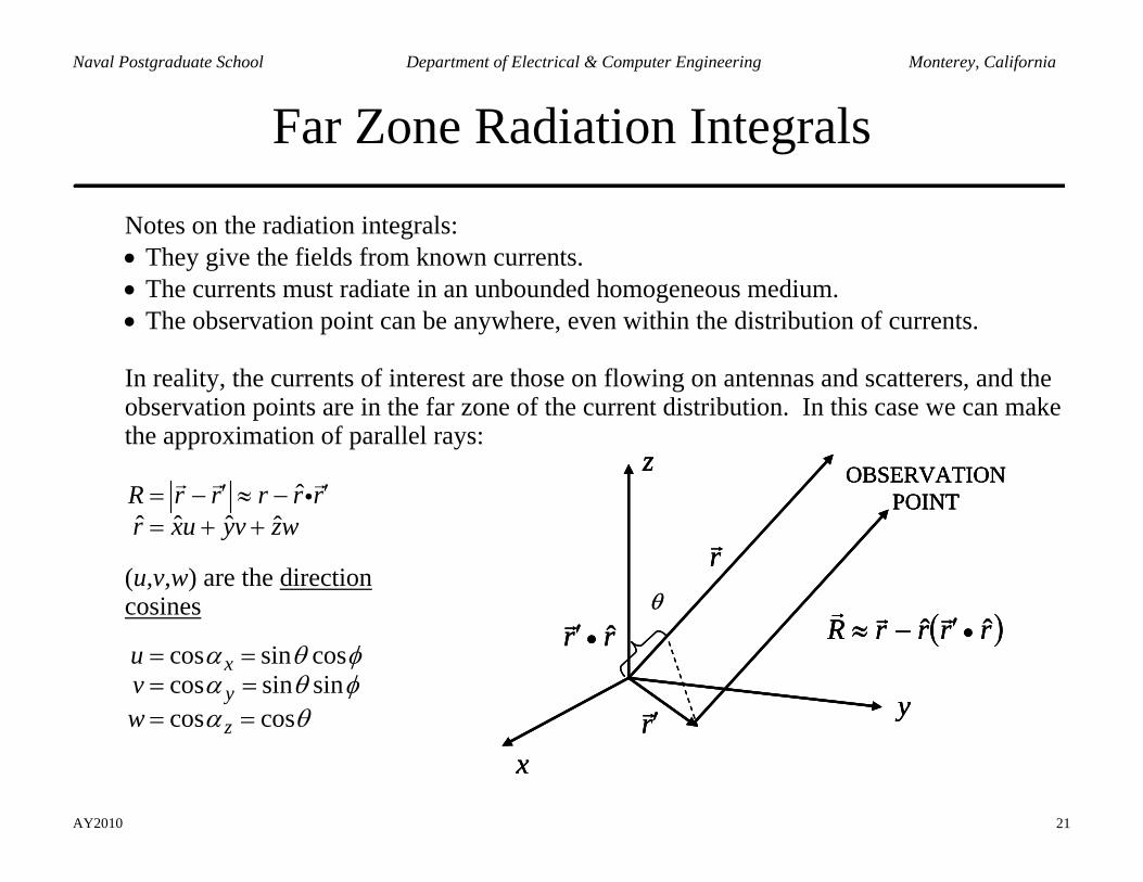
In reality, the currents of interest are those on flowing on antennas and scatterers, and the observation points are in the far zone of the current distribution. In this case we can make the approximation of parallel rays:

ˆ

ˆ ˆ ˆ ˆR r r r r rr xu yv zw

′ ′= − ≈ −= + +

i

(u,v,w) are the direction cosines

cos sin coscos sin sincos cos

xy

z

uvw

α θ φα θ φα θ

= == == =

x

y

z

r′

r

OBSERVATIONPOINT

( )rrrrR ˆˆ •′−≈rr ˆ•′θ

x

y

z

r′

r

OBSERVATIONPOINT

( )rrrrR ˆˆ •′−≈rr ˆ•′

x

y

z

r′

r

OBSERVATIONPOINT

( )rrrrR ˆˆ •′−≈rr ˆ•′θ

AY2010 22


Far Zone Radiation Integrals

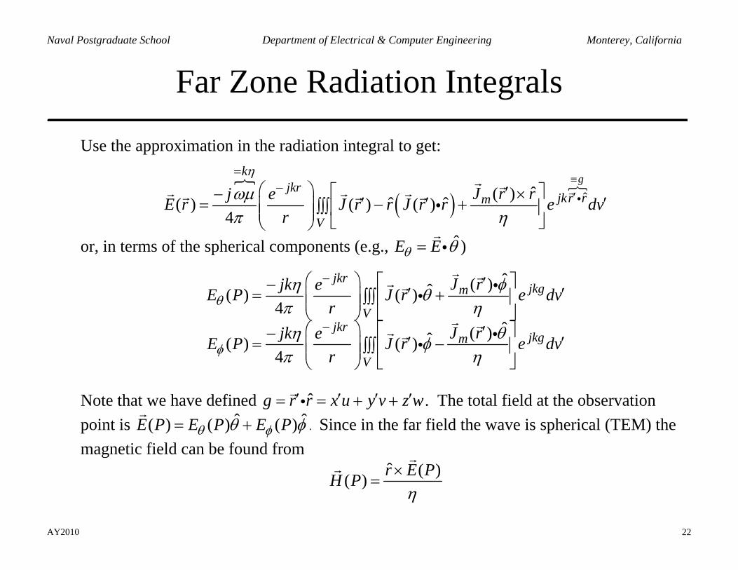
Use the approximation in the radiation integral to get:

( ) ˆˆ( )ˆ ˆ( ) ( ) ( )4

gk

jkrjkr rm

V

J r rj eE r J r r J r r e dvr

η

ωµπ η

≡=

−′⎛ ⎞ ⎡ ⎤′ ×− ′ ′ ′= − +⎜ ⎟ ∫∫∫ ⎢ ⎥⎜ ⎟ ⎣ ⎦⎝ ⎠

ii

or, in terms of the spherical components (e.g., ˆE Eθ θ= i )

ˆ( )ˆ( ) ( )4

ˆ( )ˆ( ) ( )4

jkrjkgm

Vjkr

jkgm

V

J rjk eE P J r e dvr

J rjk eE P J r e dvr

θ

φ

φη θπ η

θη φπ η

−

−

⎛ ⎞ ⎡ ⎤′− ′ ′= +⎜ ⎟ ∫∫∫ ⎢ ⎥⎜ ⎟ ⎣ ⎦⎝ ⎠⎛ ⎞ ⎡ ⎤′− ′ ′= −⎜ ⎟ ∫∫∫ ⎢ ⎥⎜ ⎟ ⎣ ⎦⎝ ⎠

ii

ii

Note that we have defined ˆg r r x u y v z w′ ′ ′ ′= = + +i . The total field at the observation point is ˆ ˆ( ) ( ) ( )E P E P E Pθ φθ φ= + . Since in the far field the wave is spherical (TEM) the magnetic field can be found from

ˆ ( )( ) r E PH Pη

×=

AY2010 23


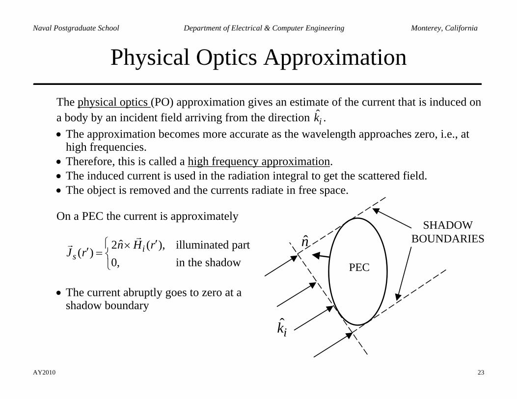
Physical Optics Approximation

The physical optics (PO) approximation gives an estimate of the current that is induced on a body by an incident field arriving from the direction ik . • The approximation becomes more accurate as the wavelength approaches zero, i.e., at

high frequencies. • Therefore, this is called a high frequency approximation. • The induced current is used in the radiation integral to get the scattered field. • The object is removed and the currents radiate in free space.

On a PEC the current is approximately

ˆ2 ( ), illuminated part( )

0, in the shadowi

sn H r

J r⎧ ′×′ = ⎨⎩

• The current abruptly goes to zero at a

shadow boundary

PEC

SHADOWBOUNDARIES

ik

n

AY2010 24


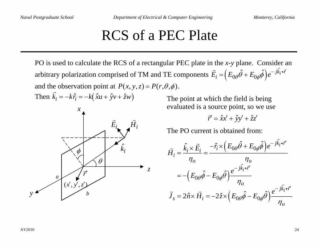
RCS of a PEC Plate

PO is used to calculate the RCS of a rectangular PEC plate in the x-y plane. Consider an arbitrary polarization comprised of TM and TE components ( ) ˆ

0 0ˆ ˆ ijk r

iE E E eθ φθ φ −= + i and the observation point at ( , , ) ( , , )P x y z P r θ φ= . Then ( )ˆ ˆ ˆ ˆi ik kr k xu yv zw= − = − + +

ik

iE iH

y

x

zθ

φ

r′

( , , )x y z′ ′ ′a

b

The point at which the field is being evaluated is a source point, so we use

ˆ ˆ ˆr xx yy zz′ ′ ′ ′= + +

The PO current is obtained from:

( )

( )

( )

ˆ0 0

ˆ

0 0ˆ

0 0

ˆ ˆˆˆ

ˆ ˆ

ˆ ˆˆ ˆ2 2

i

i

i

jk rii i

io o

jk r

ojk r

s io

r E E ek EH

eE E

eJ n H z E E

θ φ

θ φ

θ φ

θ φ

η η

φ θη

φ θη

′−

′−

′−

− × +×= =

= − −

= × = − × −

i

i

i

AY2010 25


RCS of a PEC Plate

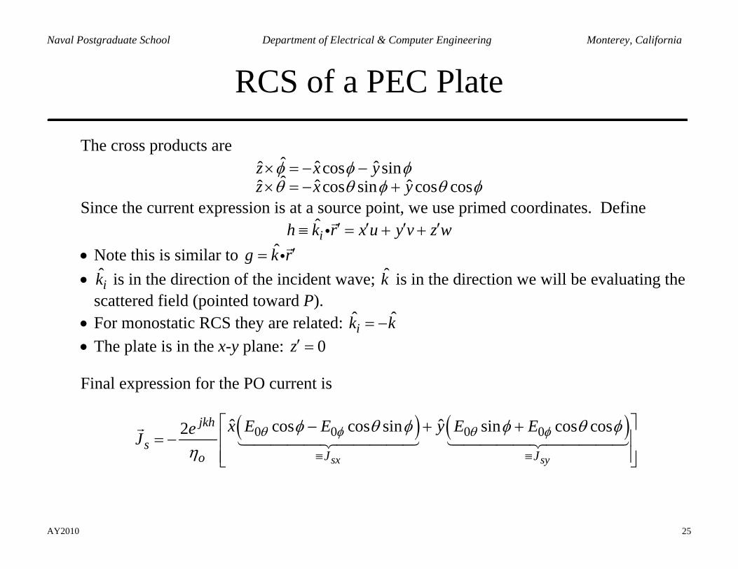
The cross products are

ˆ ˆ ˆˆ cos sinˆ ˆ ˆˆ cos sin cos cos

z x yz x y

φ φ φθ θ φ θ φ

× = − −× = − +

Since the current expression is at a source point, we use primed coordinates. Define ih k r x u y v z w′ ′ ′ ′≡ = + +i

• Note this is similar to ˆg k r′= i • ik is in the direction of the incident wave; k is in the direction we will be evaluating the

scattered field (pointed toward P). • For monostatic RCS they are related: ˆ ˆ

ik k= − • The plate is in the x-y plane: 0z′ =

Final expression for the PO current is

( ) ( )0 0 0 0ˆ ˆcos cos sin sin cos cos2

sx sy

jkh

sJ Jo

x E E y E EeJ θ φ θ φφ θ φ φ θ φη ≡ ≡

⎡ ⎤− + += − ⎢ ⎥

⎢ ⎥⎣ ⎦

AY2010 26


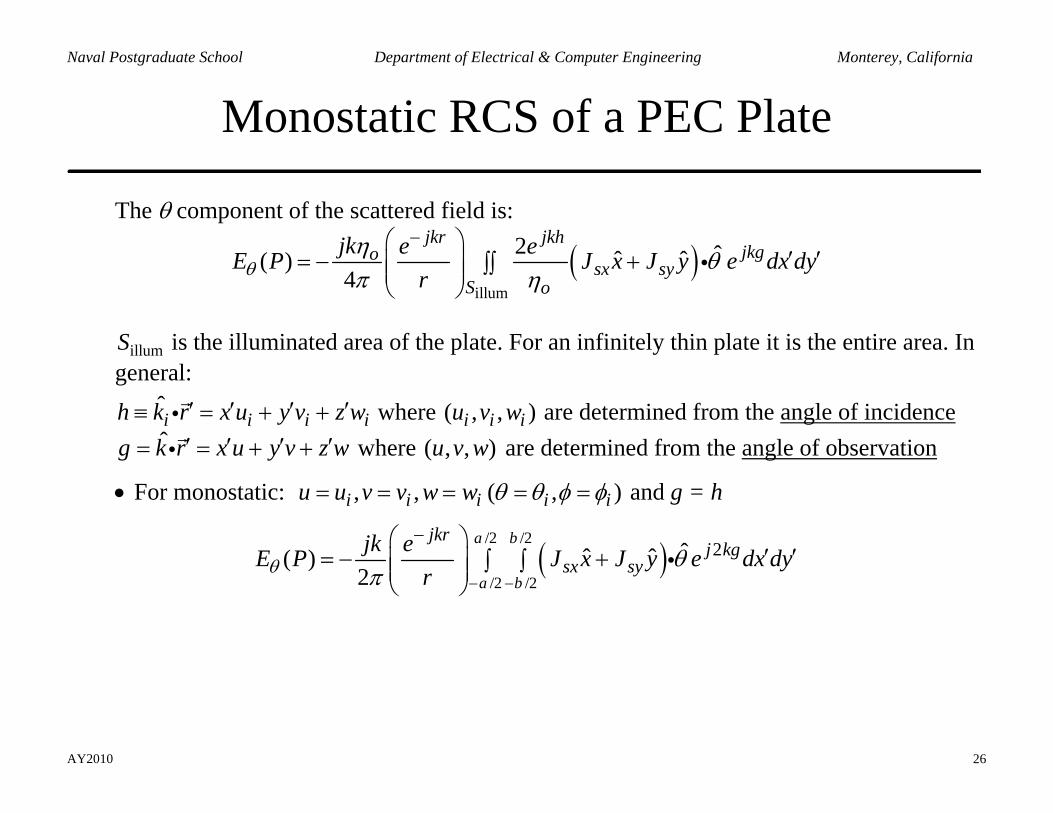
Monostatic RCS of a PEC Plate

The θ component of the scattered field is:

( )illum

2 ˆˆ ˆ( )4

jkr jkhjkgo

sx syS o

jk e eE P J x J y e dx dyrθ

η θπ η

−⎛ ⎞′ ′= − +⎜ ⎟ ∫∫⎜ ⎟

⎝ ⎠i

illumS is the illuminated area of the plate. For an infinitely thin plate it is the entire area. In

general:

i i i ih k r x u y v z w′ ′ ′ ′≡ = + +i where ( , , )i i iu v w are determined from the angle of incidence ˆg k r x u y v z w′ ′ ′ ′= = + +i where ( , , )u v w are determined from the angle of observation

• For monostatic: , , ( , )i i i i iu u v v w w θ θ φ φ= = = = = and g = h

( )/2 /2

/2 /2

2ˆˆ ˆ( )2

a b

a b

jkrj kg

sx syjk eE P J x J y e dx dy

rθ θπ − −

−⎛ ⎞′ ′= − +⎜ ⎟ ∫ ∫⎜ ⎟

⎝ ⎠i

AY2010 27



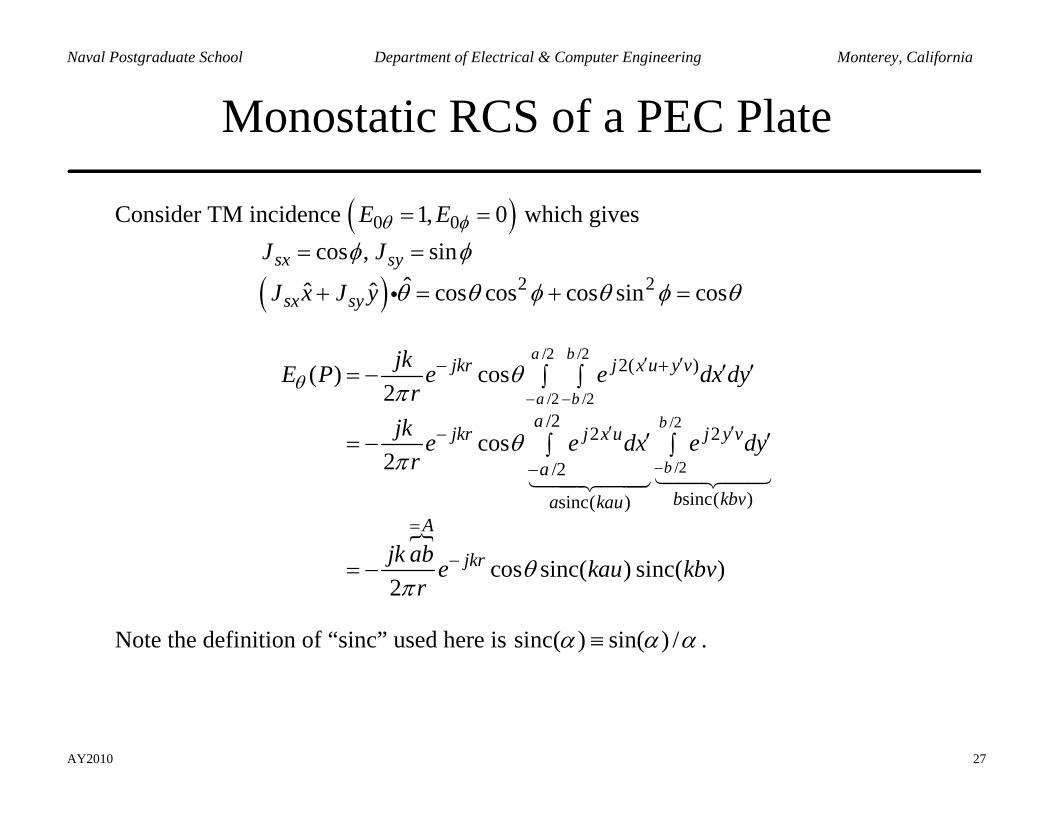
Consider TM incidence ( )0 01, 0E Eθ φ= = which gives cos , sinsx syJ Jφ φ= =

( ) 2 2ˆˆ ˆ cos cos cos sin cossx syJ x J y θ θ φ θ φ θ+ = + =i

/2 /2

/2 /2/2

/2

2( )

/22 2

/2sinc( )sinc( )

( ) cos2

cos2

cos sinc( ) sinc( )2

a b

a bb

b

jkr j x u y v

ajkr j x u j y v

ab kbva kau

A

jkr

jkE P e e dx dyr

jk e e dx e dyr

jk ab e kau kbvr

θ θπ

θπ

θπ

− −

−

′ ′− +

′ ′−

−

=

−

′ ′= − ∫ ∫

′ ′= − ∫ ∫

= −

Note the definition of “sinc” used here is sinc( ) sin( ) /α α α≡ .

AY2010 28



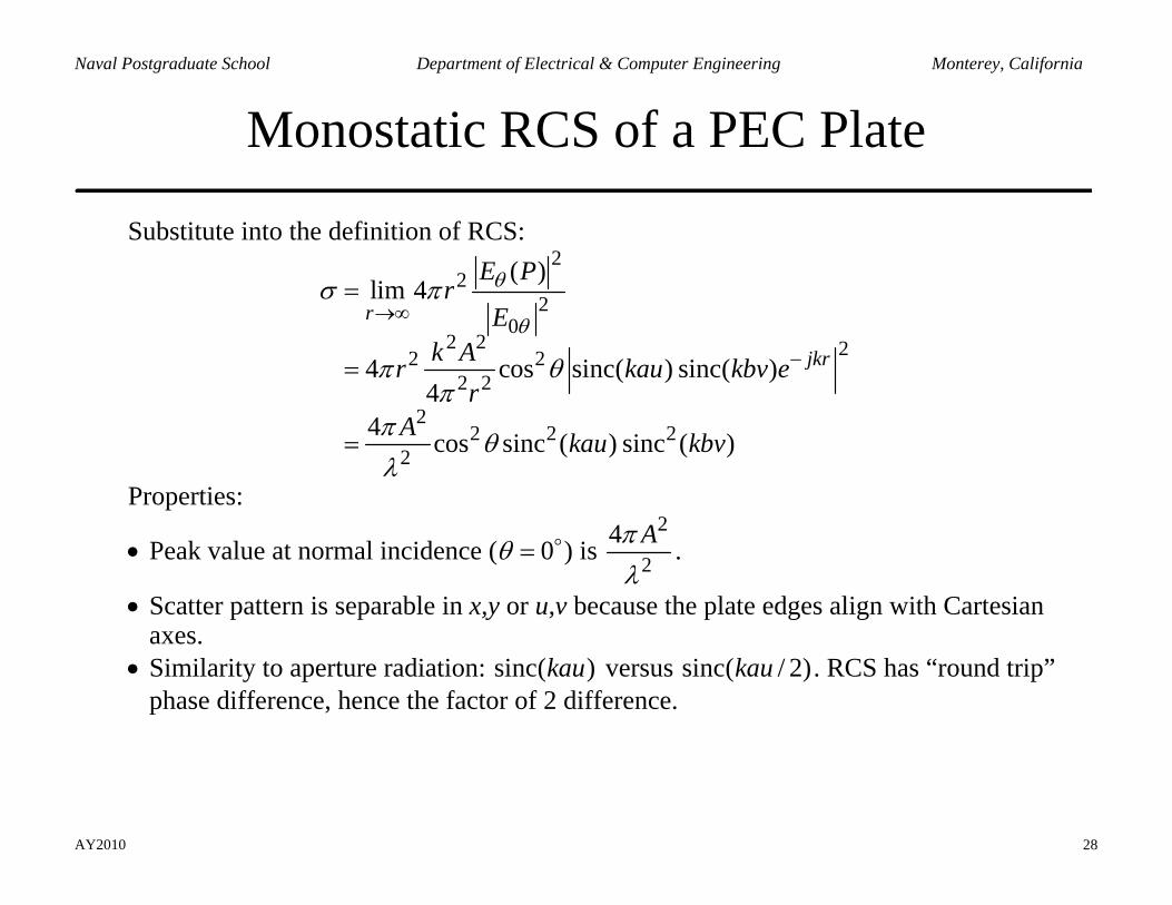
Substitute into the definition of RCS:

22

20

2 2 22 22 2

22 2 2

2

( )lim 4

4 cos sinc( ) sinc( )4

4 cos sinc ( ) sinc ( )

r

jkr

E Pr

Ek Ar kau kbv e

rA kau kbv

θ

θ

σ π

π θπ

π θλ

→∞

−

=

=

=

Properties:

• Peak value at normal incidence ( 0θ = ) is 2

24 Aπ

λ.

• Scatter pattern is separable in x,y or u,v because the plate edges align with Cartesian axes.

• Similarity to aperture radiation: sinc( )kau versus sinc( / 2)kau . RCS has “round trip” phase difference, hence the factor of 2 difference.

AY2010 29


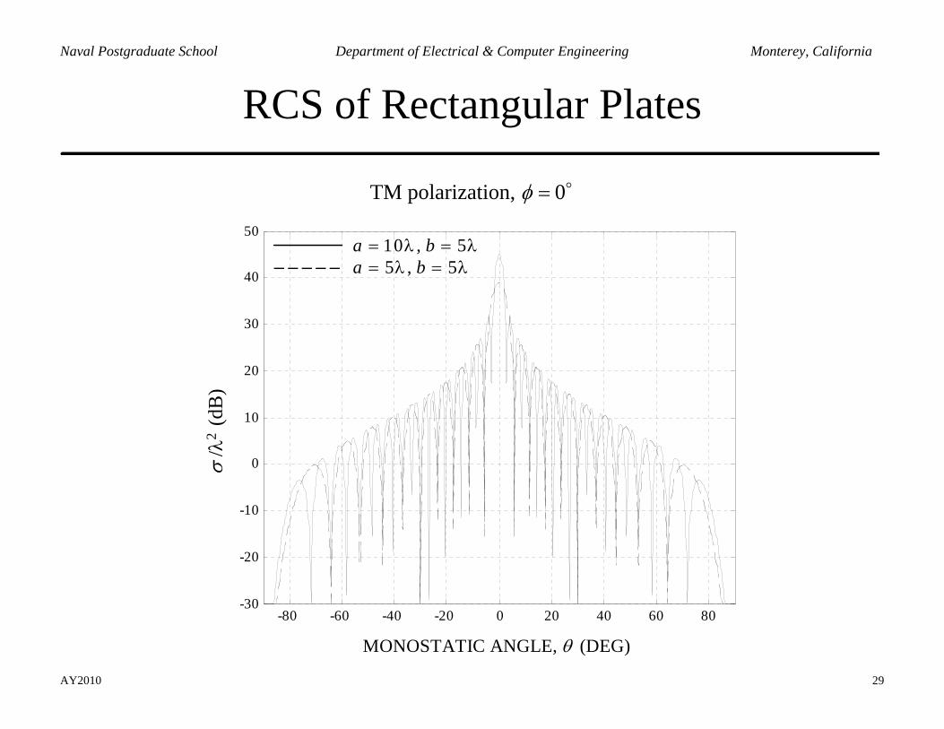
RCS of Rectangular Plates

TM polarization, 0φ =

-80 -60 -40 -20 0 20 40 60 80-30

-20

-10

0

10

20

30

40

50 σ

/λ2

(dB

)10 , 55 , 5

a ba b

= λ = λ= λ = λ

MONOSTATIC ANGLE, (DEG)θ

AY2010 30


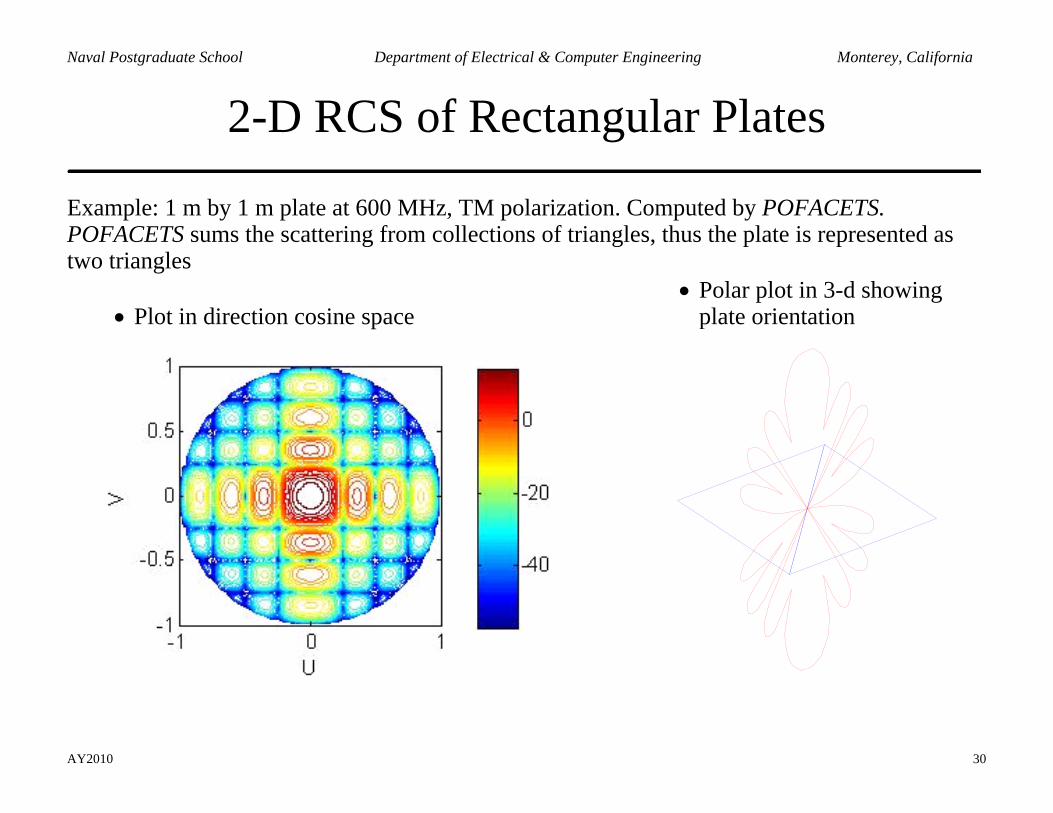
2-D RCS of Rectangular Plates

Example: 1 m by 1 m plate at 600 MHz, TM polarization. Computed by POFACETS. POFACETS sums the scattering from collections of triangles, thus the plate is represented as two triangles

• Plot in direction cosine space

• Polar plot in 3-d showing plate orientation

AY2010 31


Tapered Current Distributions

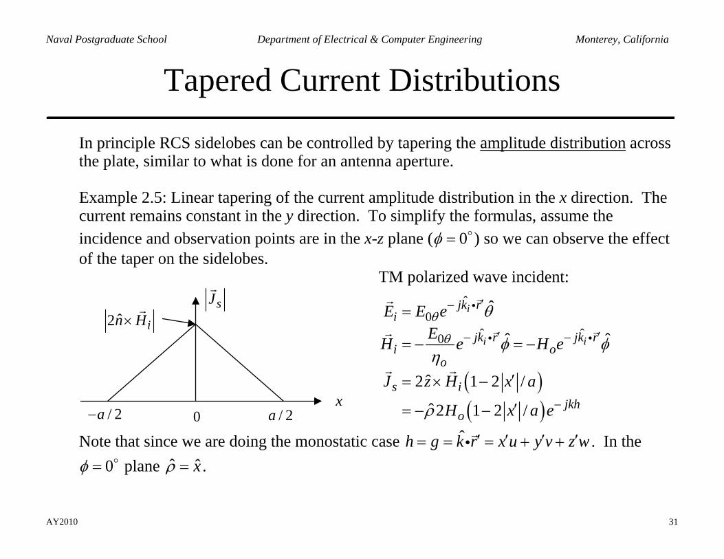
In principle RCS sidelobes can be controlled by tapering the amplitude distribution across the plate, similar to what is done for an antenna aperture.

Example 2.5: Linear tapering of the current amplitude distribution in the x direction. The current remains constant in the y direction. To simplify the formulas, assume the incidence and observation points are in the x-z plane ( 0φ = ) so we can observe the effect of the taper on the sidelobes.

sJ

ˆ2 in H×

/ 2a− / 2ax

0

TM polarized wave incident:

( )( )

ˆ0

ˆ ˆ0

ˆ

ˆ ˆ

ˆ2 1 2 /

ˆ2 1 2 /

i

i i

jk ri

jk r jk ri o

o

s ijkh

o

E E eEH e H e

J z H x a

H x a e

θ

θ

θ

φ φη

ρ

′−

′ ′− −

−

=

= − = −

′= × −

′= − −

i

i i

Note that since we are doing the monostatic case ˆh g k r x u y v z w′ ′ ′ ′= = = + +i . In the 0φ = plane ˆ xρ = .

AY2010 32


Tapered Current Distributions

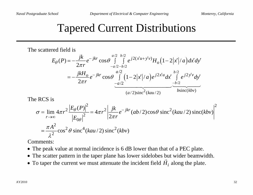
The scattered field is

( )

( )

/2 /2

/2 /2/2

/2

2

2( )

/22 2

/2sinc( )( / 2)sinc ( / 2)

( ) cos 1 2 /2

cos 1 2 /2

a b

a bb

b

jkr j x u y vo

ajkr j x u j y vo

ab kbva kau

jkE P e e H x a dx dyr

jkH e x a e dx e dyr

θ θπ

θπ

− −

−

′ ′− +

′ ′−

−

′ ′ ′= − −∫ ∫

′ ′ ′= − −∫ ∫

The RCS is 2 2

2 2 22

02

2 4 22

( )lim 4 4 ( / 2)cos sinc ( / 2) sinc( )

2

cos sinc ( / 2) sinc ( )

jkrr

E P jkr r e ab kau kbvrE

A kau kbv

θ

θ

σ π π θπ

π θλ

−

→∞= =

=

Comments: • The peak value at normal incidence is 6 dB lower than that of a PEC plate. • The scatter pattern in the taper plane has lower sidelobes but wider beamwidth. • To taper the current we must attenuate the incident field iH along the plate.

AY2010 33


Null Field Hypothesis

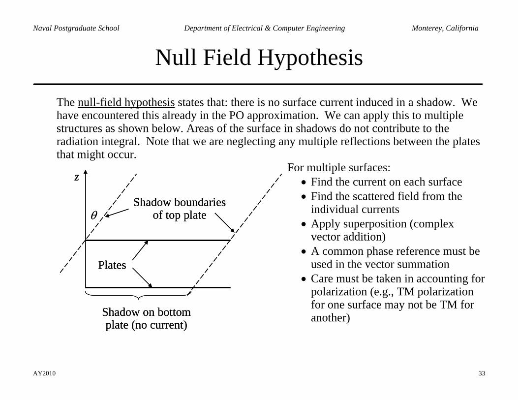
The null-field hypothesis states that: there is no surface current induced in a shadow. We have encountered this already in the PO approximation. We can apply this to multiple structures as shown below. Areas of the surface in shadows do not contribute to the radiation integral. Note that we are neglecting any multiple reflections between the plates that might occur.

θ Shadow boundaries

of top plate

Plates

Shadow on bottomplate (no current)

z

θ Shadow boundaries

of top plate

Plates

Shadow on bottomplate (no current)

z

For multiple surfaces: • Find the current on each surface • Find the scattered field from the

individual currents • Apply superposition (complex

vector addition) • A common phase reference must be

used in the vector summation • Care must be taken in accounting for

polarization (e.g., TM polarization for one surface may not be TM for another)

AY2010 34


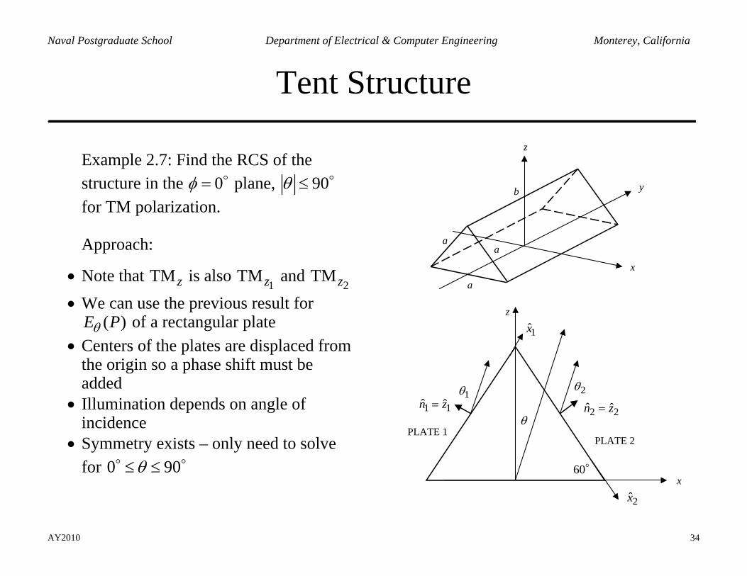
Tent Structure

Example 2.7: Find the RCS of the structure in the 0φ = plane, 90θ ≤ for TM polarization.

Approach:

• Note that TM z is also 1

TMz and 2

TMz • We can use the previous result for

( )E Pθ of a rectangular plate • Centers of the plates are displaced from

the origin so a phase shift must be added

• Illumination depends on angle of incidence

• Symmetry exists – only need to solve for 0 90θ≤ ≤

a

aa

b

z

x

y

z

x

PLATE 2 PLATE 1

θ

2θ1θ

1 1ˆ ˆn z=2 2ˆ ˆn z=

2x

1x

60

AY2010 35


Tent Structure

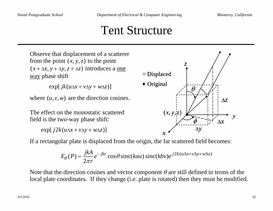
Observe that displacement of a scatterer from the point ( , , )x y z to the point ( , , )x x y y z z∆ ∆ ∆+ + + introduces a one way phase shift

exp[ ( )]jk u x v y w z∆ ∆ ∆+ +

where ( , , )u v w are the direction cosines.

The effect on the monostatic scattered field is the two-way phase shift:

exp[ 2 ( )]j k u x v y w z∆ ∆ ∆+ +

x∆y∆

z∆

z

y

x

Original

Displaced

θ

( , , )x y zφ x∆

y∆

z∆

z

y

x

Original

Displaced

θ

( , , )x y zφ

If a rectangular plate is displaced from the origin, the far scattered field becomes:

2 ( )( ) cos sinc( ) sinc( )2

jkr j k u x v y w zjkAE P e kau kbv erθ θ

π− ∆ + ∆ + ∆=

Note that the direction cosines and vector component θ are still defined in terms of the local plate coordinates. If they change (i.e. plate is rotated) then they must be modified.

AY2010 36


Tent Structure

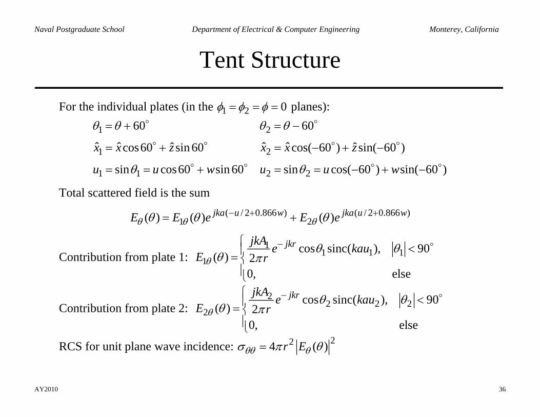
For the individual plates (in the 1 2 0φ φ φ= = = planes):

1 2

1 2

1 1 2 2

60 60

ˆ ˆ ˆ ˆˆ ˆcos60 sin 60 cos( 60 ) sin( 60 )

sin cos60 sin 60 sin cos( 60 ) sin( 60 )

x x z x x z

u u w u u w

θ θ θ θ

θ θ

= + = −

= + = − + −

= = + = = − + −

Total scattered field is the sum

( / 2 0.866 ) ( / 2 0.866 )1 2( ) ( ) ( )jka u w jka u wE E e E eθ θ θθ θ θ− + += +

Contribution from plate 1: 1

1 1 11

cos sinc( ), 90( ) 2

0, else

jkrjkA e kauE rθ

θ θθ π

−⎧ <⎪= ⎨⎪⎩

Contribution from plate 2: 2

2 2 22

cos sinc( ), 90( ) 2

0, else

jkrjkA e kauE rθ

θ θθ π

−⎧ <⎪= ⎨⎪⎩

RCS for unit plane wave incidence: 224 ( )r Eθθ θσ π θ=

AY2010 37


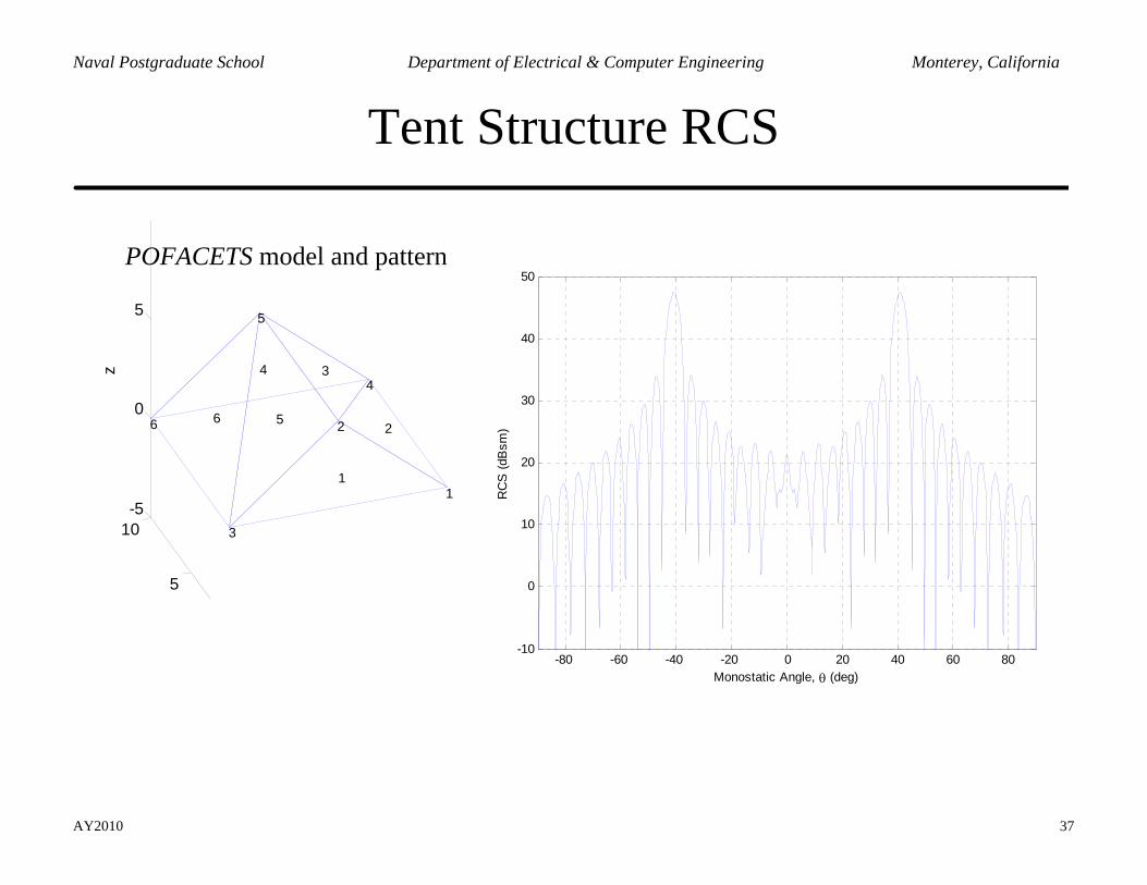
Tent Structure RCS

POFACETS model and pattern

5

10-5

0

5

1

2

4

1

2

3

5

4

5

3

66

z

-80 -60 -40 -20 0 20 40 60 80-10

0

10

20

30

40

50

Monostatic Angle, θ (deg)

RC

S (d

Bsm

)

AY2010 38


Arrays of Scatterers

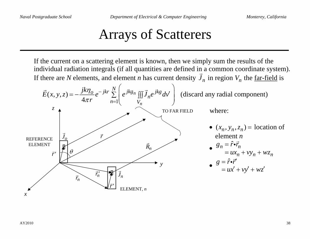
If the current on a scattering element is known, then we simply sum the results of the individual radiation integrals (if all quantities are defined in a common coordinate system). If there are N elements, and element n has current density nJ in region nV the far-field is

1( , , ) (discard any radial component)

4n

n

N jkgjkr jkgon

n V

jkE x y z e e J e dvr

ηπ

−

=

⎛ ⎞′= − ⎜ ⎟∑ ∫∫∫⎜ ⎟

⎝ ⎠

x

y

z

r n

r

R n

′ r n

′ r

′ r

J o

J n

θ

TO FAR FIELD

REFERENCEELEMENT

ELEMENT, n

where: • ( , , )n n nx y z = location of

element n

• ˆn nn n n

g r rux vy wz

== + +

i

• ˆg r rux vy wz

′=′ ′ ′= + +

i

AY2010 39


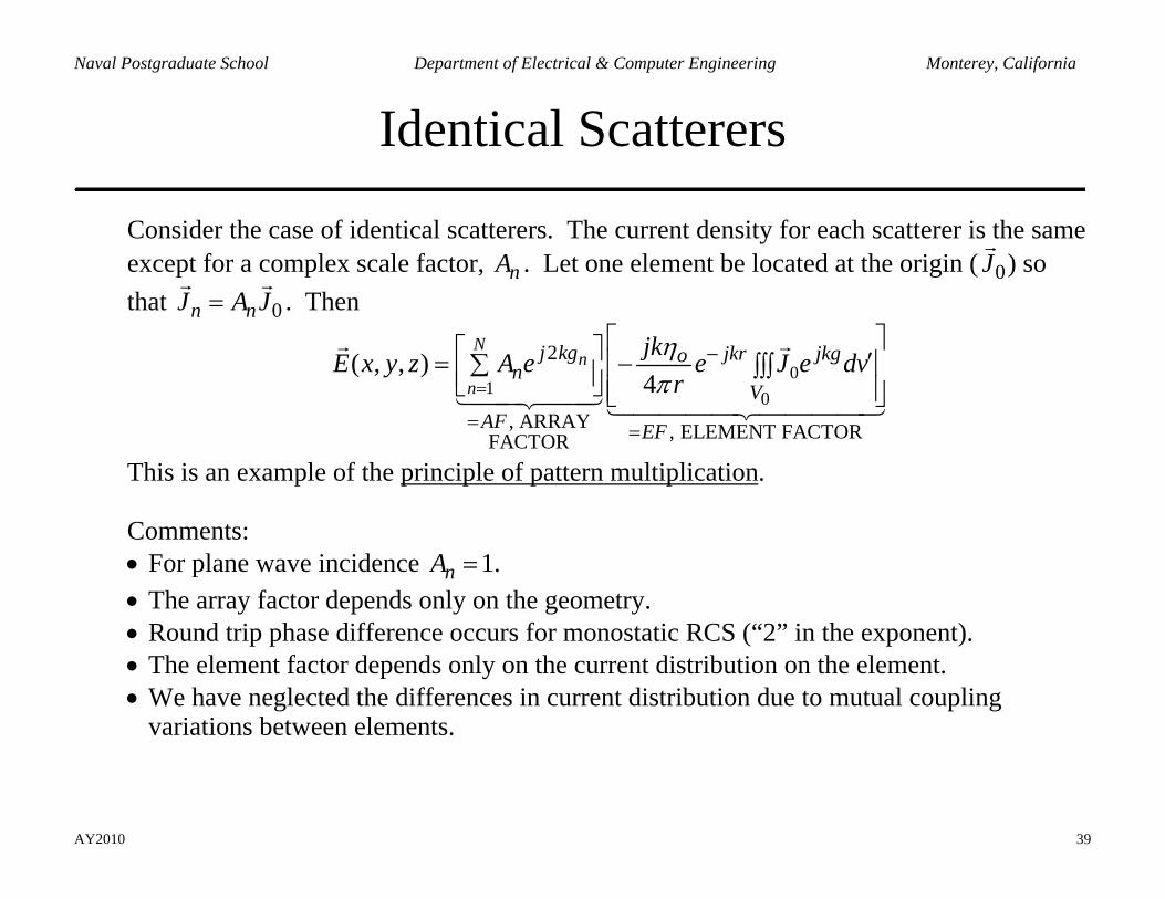
Identical Scatterers

Consider the case of identical scatterers. The current density for each scatterer is the same except for a complex scale factor, nA . Let one element be located at the origin ( 0J ) so that 0n nJ A J= . Then

01 0

2

, ARRAY , ELEMENT FACTORFACTOR

( , , )4

Nn

n

j kg jkr jkgon

VAF EF

jkE x y z A e e J e dvr

ηπ=

−

= =

⎡ ⎤⎡ ⎤ ′= −∑ ⎢ ⎥∫∫∫⎢ ⎥⎣ ⎦ ⎢ ⎥⎣ ⎦

This is an example of the principle of pattern multiplication. Comments: • For plane wave incidence 1nA = . • The array factor depends only on the geometry. • Round trip phase difference occurs for monostatic RCS (“2” in the exponent). • The element factor depends only on the current distribution on the element. • We have neglected the differences in current distribution due to mutual coupling

variations between elements.

AY2010 40


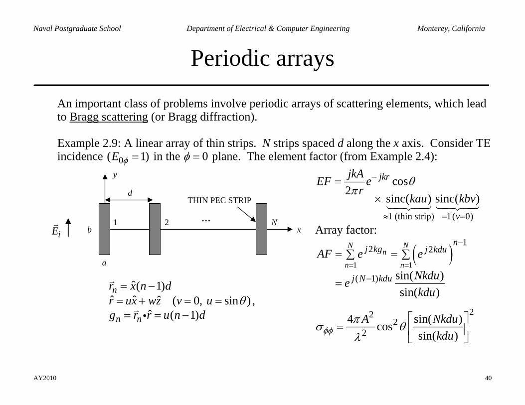
Periodic arrays

An important class of problems involve periodic arrays of scattering elements, which lead to Bragg scattering (or Bragg diffraction). Example 2.9: A linear array of thin strips. N strips spaced d along the x axis. Consider TE incidence 0( 1)E φ = in the 0φ = plane. The element factor (from Example 2.4):

a

b

d

y

x1 2 N

iE...

THIN PEC STRIP

ˆ( 1)ˆ ˆ ˆ ( 0, sin )

ˆ ( 1)

n

n n

r x n dr ux wz v ug r r u n d

θ= −

= + = == = −i

,

1 (thin strip) 1( 0)

cos2

sinc( ) sinc( )

jkr

v

jkAEF er

kau kbvθ

π−

≈ = =

=×

Array factor:

( )1 1

12 2

( 1) sin( )sin( )

N Nn

n n

nj kg j kdu

j N kdu

AF e e

Nkduekdu

= =

−

−

= =∑ ∑

=

222

24 sin( )cos

sin( )A Nkdu

kduφφπσ θλ

⎡ ⎤= ⎢ ⎥

⎣ ⎦

AY2010 41


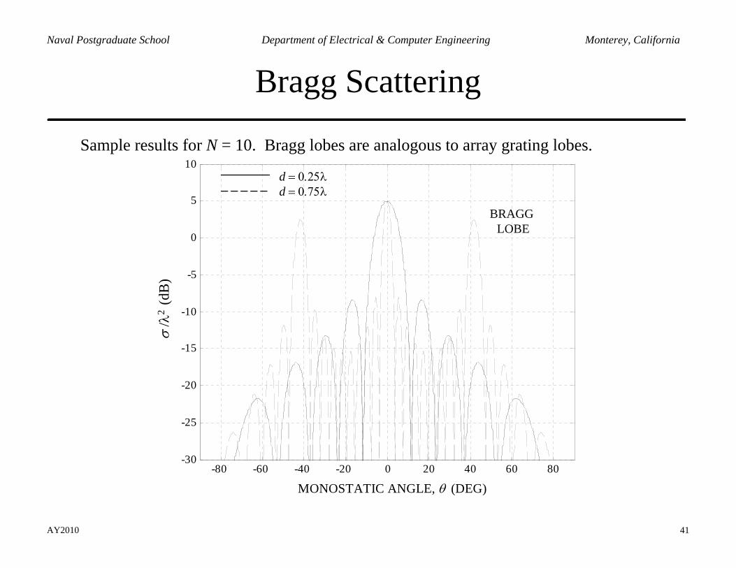
Bragg Scattering

Sample results for N = 10. Bragg lobes are analogous to array grating lobes.

-80 -60 -40 -20 0 20 40 60 80-30

-25

-20

-15

-10

-5

0

5

10

BRAGG LOBE

d = 0.25λd = 0.75λ

σ /λ

2 (d

B)


AY2010 42


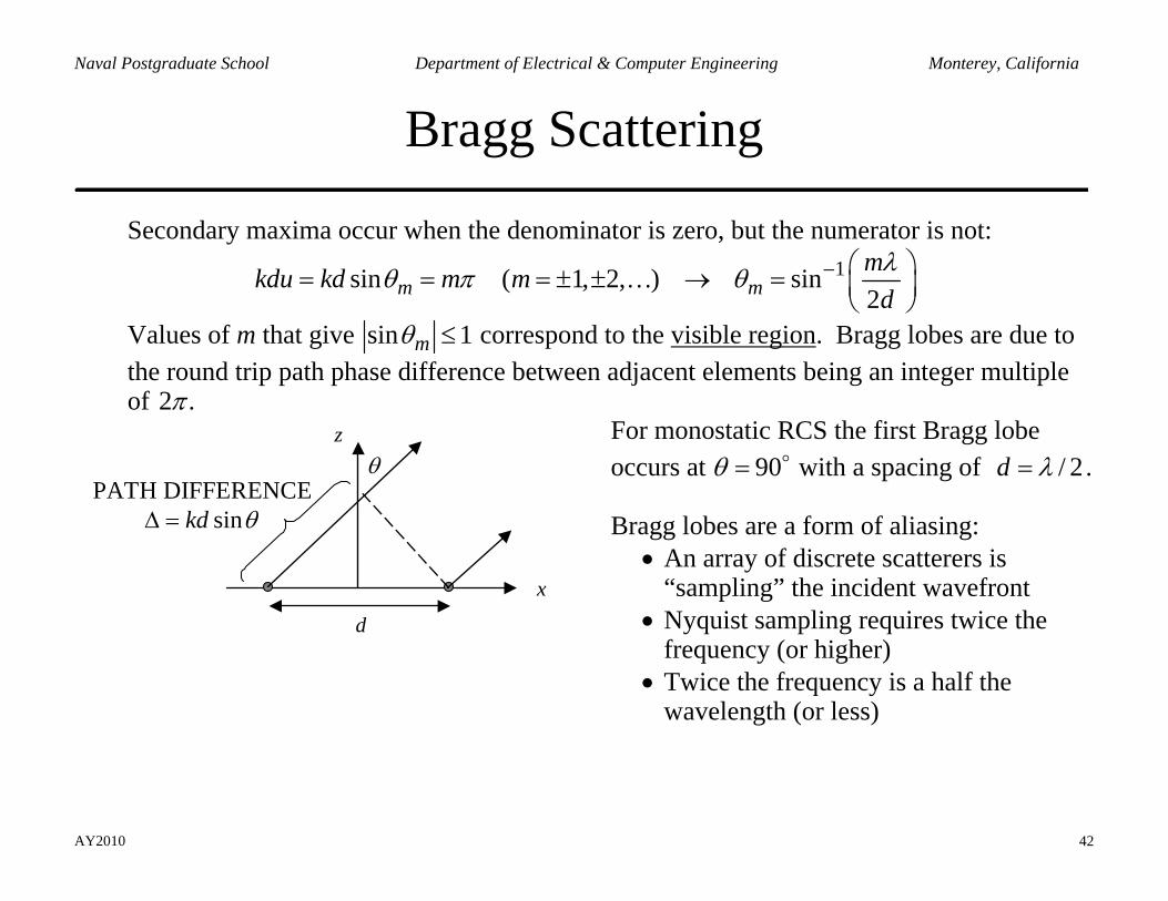
Bragg Scattering

Secondary maxima occur when the denominator is zero, but the numerator is not:

1sin ( 1, 2, ) sin2m mmkdu kd m m

dλθ π θ − ⎛ ⎞= = = ± ± → = ⎜ ⎟

⎝ ⎠…

Values of m that give sin 1mθ ≤ correspond to the visible region. Bragg lobes are due to the round trip path phase difference between adjacent elements being an integer multiple of 2 .π

d

PATH DIFFERENCEsinkd θ∆ =

x

zθ

For monostatic RCS the first Bragg lobe occurs at 90θ = with a spacing of / 2d λ= . Bragg lobes are a form of aliasing:

• An array of discrete scatterers is “sampling” the incident wavefront

• Nyquist sampling requires twice the frequency (or higher)

• Twice the frequency is a half the wavelength (or less)

AY2010 43


Bragg Diagram

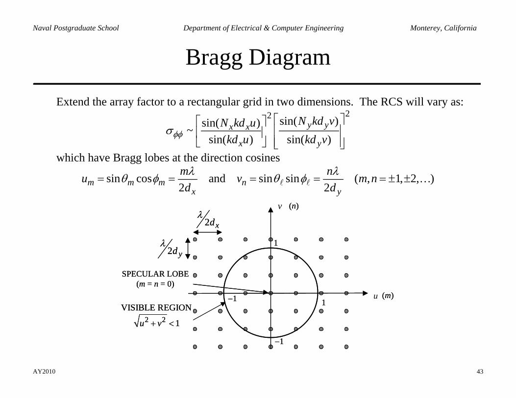
Extend the array factor to a rectangular grid in two dimensions. The RCS will vary as:

22 sin( )sin( )~sin( ) sin( )

y yx x

x y

N kd vN kd ukd u kd vφφσ

⎡ ⎤⎡ ⎤⎢ ⎥⎢ ⎥⎢ ⎥⎣ ⎦ ⎣ ⎦

which have Bragg lobes at the direction cosines

sin cos and sin sin ( , 1, 2, )2 2m m m n

x y

m nu v m nd dλ λθ φ θ φ= = = = = ± ± …

x (m)

2 xdλ

2 2VISIBLE REGION

1u v+ <

2 ydλ

y (n)

SPECULAR LOBE(m = n = 0)

1

1

−1

−1

v

ux (m)

2 xdλ

2 2VISIBLE REGION

1u v+ <

2 ydλ

y (n)

SPECULAR LOBE(m = n = 0)

1

1

−1

−1

v

u

AY2010 44


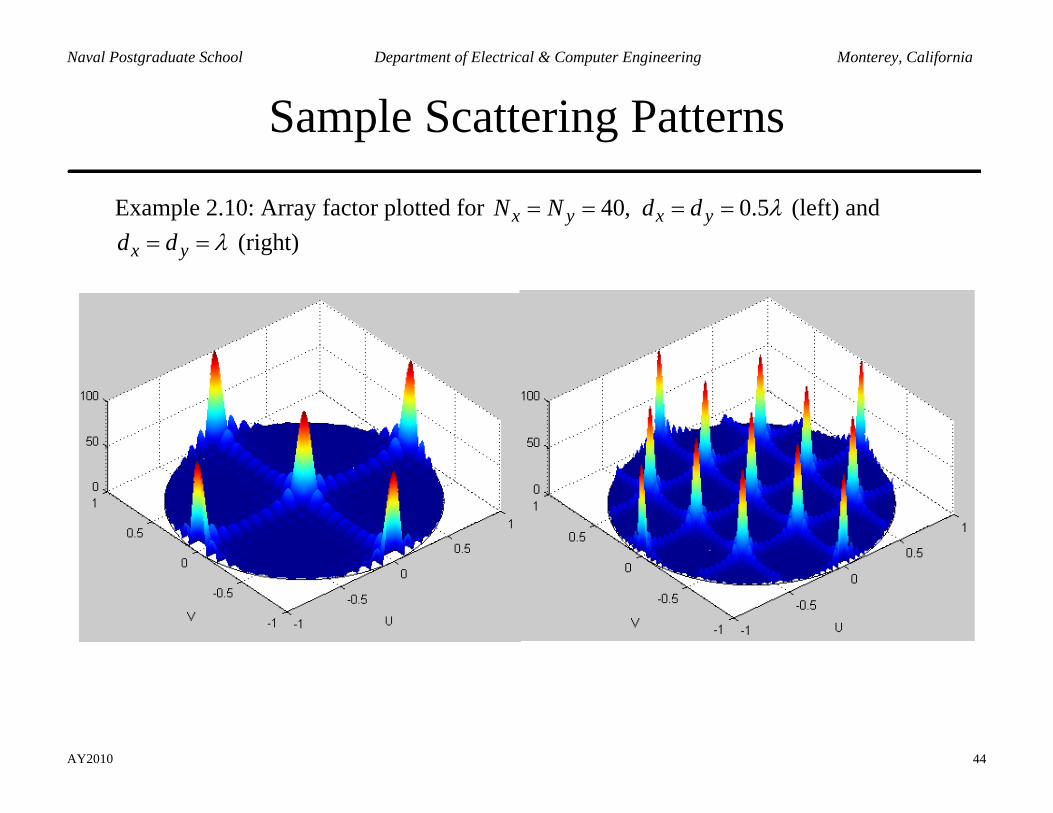
Sample Scattering Patterns

Example 2.10: Array factor plotted for 40, 0.5x y x yN N d d λ= = = = (left) and

x yd d λ= = (right)

AY2010 45


Surface Impedance

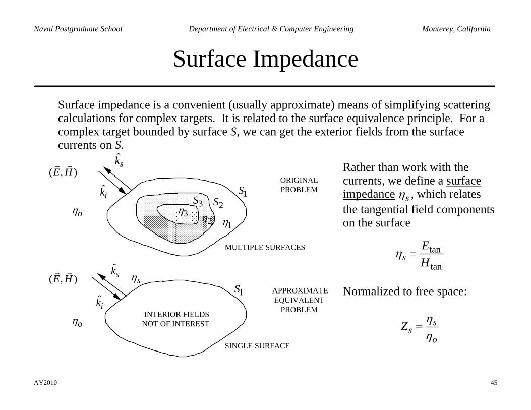
Surface impedance is a convenient (usually approximate) means of simplifying scattering calculations for complex targets. It is related to the surface equivalence principle. For a complex target bounded by surface S, we can get the exterior fields from the surface currents on S.

( , )E HORIGINAL PROBLEM

MULTIPLE SURFACES

INTERIOR FIELDSNOT OF INTEREST

ik

ˆsk

ik

ˆsk

sη

1η2η3η1S

2S3S

1S

oη

oη

( , )E H

SINGLE SURFACE

APPROXIMATEEQUIVALENT

PROBLEM

Rather than work with the currents, we define a surface impedance sη , which relates the tangential field components on the surface

tan

tans

EH

η =

Normalized to free space:

ss

oZ η

η=

AY2010 46


Surface Impedance

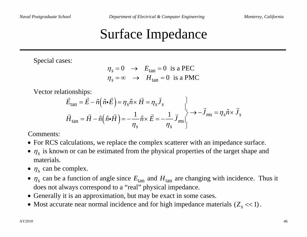
Special cases:

tan

tan

0 0 is a PEC0 is a PMC

s

s

EH

ηη

= → == ∞ → =

Vector relationships:

( )( )

tan

tan

ˆ ˆ ˆˆ1 1ˆ ˆ ˆ

s s s

ms s sms

s s

E E n n E n H JJ n J

H H n n H n E J

η ηη

η η

⎫= − = × =⎪

→ − = ×⎬= − = − × = − ⎪

⎭

i

i

Comments: • For RCS calculations, we replace the complex scatterer with an impedance surface. • sη is known or can be estimated from the physical properties of the target shape and

materials. • sη can be complex. • sη can be a function of angle since tanE and tanH are changing with incidence. Thus it

does not always correspond to a “real” physical impedance. • Generally it is an approximation, but may be exact in some cases. • Most accurate near normal incidence and for high impedance materials ( 1)sZ << .

AY2010 47


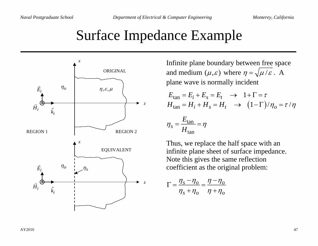
Surface Impedance Example

ik

oηiE

iH

, ,η ε µ

z

x

ik

oηiE

iH

sη

z

x

ORIGINAL

EQUIVALENT

REGION 1 REGION 2

Infinite plane boundary between free space and medium ( , )µ ε where /η µ ε= . A plane wave is normally incident

( )tan

tan

11 / /

i s t

i s t o

E E E EH H H H

τη τ η

= + = → + Γ == + = → − Γ =

tan

tans

EH

η η= =

Thus, we replace the half space with an infinite plane sheet of surface impedance. Note this gives the same reflection coefficient as the original problem:

s o o

s o o

η η η ηη η η η

− −Γ = =

+ +

AY2010 48


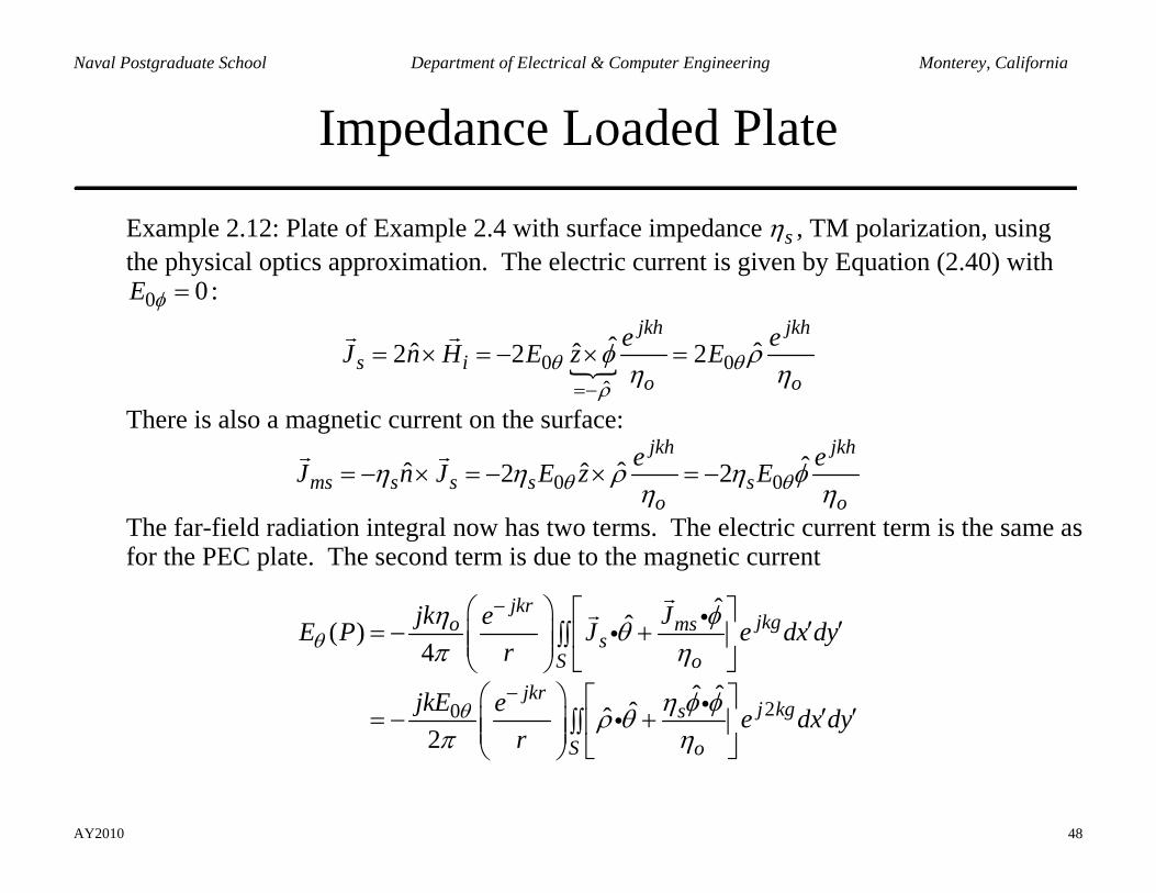
Impedance Loaded Plate

Example 2.12: Plate of Example 2.4 with surface impedance sη , TM polarization, using the physical optics approximation. The electric current is given by Equation (2.40) with

0 0E φ = :

0 0ˆ

ˆ ˆˆ ˆ2 2 2jkh jkh

s io o

e eJ n H E z Eθ θρ

φ ρη η

=−

= × = − × =

There is also a magnetic current on the surface:

0 0ˆˆˆ ˆ2 2

jkh jkh

ms s s s so o

e eJ n J E z Eθ θη η ρ η φη η

= − × = − × = −

The far-field radiation integral now has two terms. The electric current term is the same as for the PEC plate. The second term is due to the magnetic current

20

ˆˆ( )4

ˆ ˆˆˆ2

jkrjkgo ms

sS o

jkrj kgs

S o

jk JeE P J e dx dyr

jkE e e dx dyr

θ

θ

η φθπ η

η φ φρ θπ η

−

−

⎛ ⎞ ⎡ ⎤′ ′= − +⎜ ⎟ ∫∫ ⎢ ⎥⎜ ⎟ ⎣ ⎦⎝ ⎠

⎛ ⎞ ⎡ ⎤′ ′= − +⎜ ⎟ ∫∫ ⎢ ⎥⎜ ⎟ ⎣ ⎦⎝ ⎠

ii

ii

AY2010 49


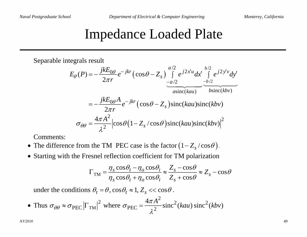
Impedance Loaded Plate

Separable integrals result

( )

( )

( )

/2

/2

/22 20

/2sinc( )sinc( )

0

2 22

( ) cos2

cos sinc( )sinc( )2

4 cos 1 / cos sinc( )sinc( )

b

b

ajkr j x u j y v

sa

b kbva kau

jkrs

s

jkEE P e Z e dx e dyr

jkE A e Z kau kbvr

A Z kau kbv

θθ

θ

θθ

θπ

θπ

πσ θ θλ

−

′ ′−

−

−

′ ′= − − ∫ ∫

= − −

= −

Comments: • The difference from the TM PEC case is the factor ( )1 / cossZ θ− . • Starting with the Fresnel reflection coefficient for TM polarization

TMcos cos cos coscos cos cos

s t o i ss

s t o i s

Z ZZ

η θ η θ θ θη θ η θ θ

− −Γ = ≈ ≈ −

+ +

under the conditions , cos 1, cost t sZθ θ θ θ= ≈ << .

• Thus TM2

PECθθσ σ≈ Γ where 2

2 2PEC 2

4 sinc ( ) sinc ( )A kau kbvπσλ

=

AY2010 50


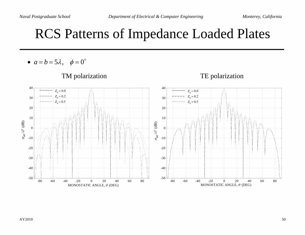
RCS Patterns of Impedance Loaded Plates

• 5 , 0a b λ φ= = =

TM polarization TE polarization

-80 -60 -40 -20 0 20 40 60 80-50

-40

-30

-20

-10

0

10

20

30

40

σ

θθ /λ

2 (d

B)


Zs = 0.0

Zs = 0.2

Zs = 0.5

-80 -60 -40 -20 0 20 40 60 80

-50

-40

-30

-20

-10

0

10

20

30

40

σ φ

φ /λ2

(dB

)


Zs = 0.0

Zs = 0.2

Zs = 0.5

AY2010 51


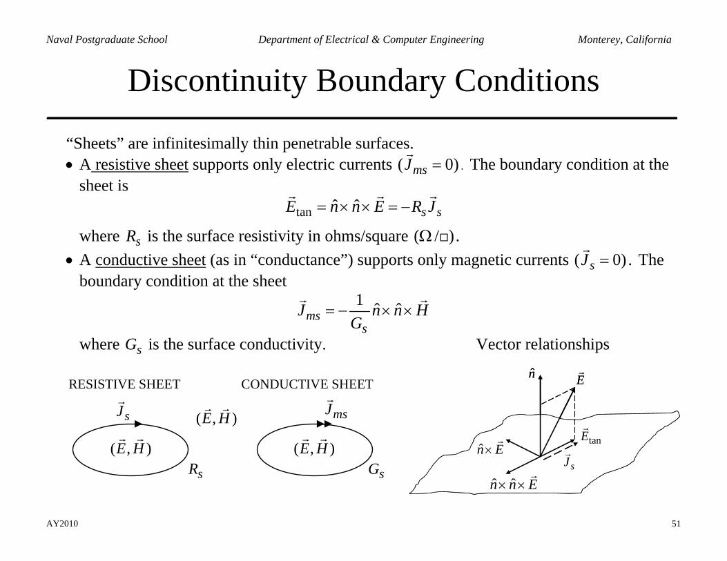
Discontinuity Boundary Conditions

“Sheets” are infinitesimally thin penetrable surfaces. • A resistive sheet supports only electric currents ( 0)msJ = . The boundary condition at the

sheet is tan ˆ ˆ s sE n n E R J= × × = −

where sR is the surface resistivity in ohms/square ( / )Ω . • A conductive sheet (as in “conductance”) supports only magnetic currents ( 0)sJ = . The

boundary condition at the sheet 1 ˆ ˆms

sJ n n H

G= − × ×

where sG is the surface conductivity. Vector relationships

sJ

sR

msJ

sG

( , )E H

( , )E H( , )E H

RESISTIVE SHEET CONDUCTIVE SHEET

tanE

En

n E×

ˆ ˆn n E× ×sJ

tanE

En

n E×

ˆ ˆn n E× ×sJ

AY2010 52


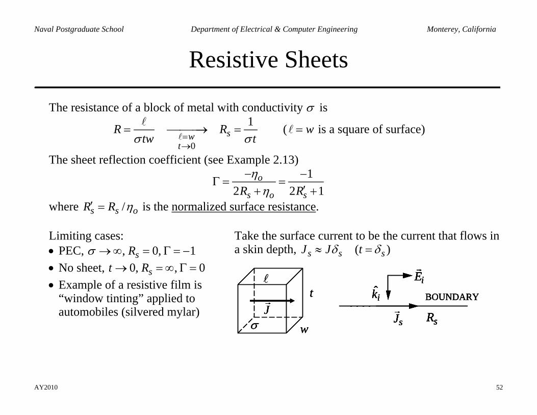
Resistive Sheets

The resistance of a block of metal with conductivity σ is

0

1sw

t

R Rtw tσ σ=

→

= ⎯⎯⎯→ = ( w= is a square of surface)

The sheet reflection coefficient (see Example 2.13) 1

2 2 1o

s o sR Rη

η− −

Γ = =′+ +

where /s s oR R η′ = is the normalized surface resistance.

Limiting cases: • PEC, , 0, 1sRσ → ∞ = Γ = − • No sheet, 0, , 0st R→ = ∞ Γ = • Example of a resistive film is

“window tinting” applied to automobiles (silvered mylar)

Take the surface current to be the current that flows in a skin depth, ( )s s sJ J tδ δ≈ =

σ

Jw

t

E i

ˆ k i BOUNDARY

J s sRσJ

w

t

σJ

w

t

E i

ˆ k i BOUNDARY

J s sR

E iˆ k i BOUNDARY

J s sR

E iˆ k i BOUNDARY

J s sR

AY2010 53


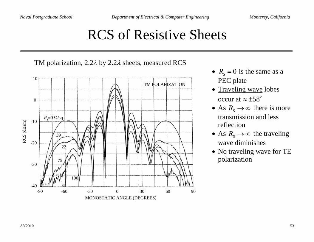
RCS of Resistive Sheets

TM polarization, 2.2λ by 2.2λ sheets, measured RCS

-90 -60 -30 0 30 60 90MONOSTATIC ANGLE (DEGREES)

RC

S (d

Bsm

)

10

0

-10

-20

-30

-40

Rs=0 Ω/sq

39

22

100

75

TM POLARIZATION

• 0sR = is the same as a PEC plate

• Traveling wave lobes occur at 58≈ ±

• As sR → ∞ there is more transmission and less reflection

• As sR → ∞ the traveling wave diminishes

• No traveling wave for TE polarization

AY2010 54


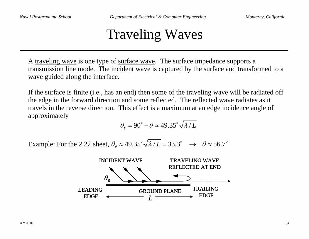
Traveling Waves

A traveling wave is one type of surface wave. The surface impedance supports a transmission line mode. The incident wave is captured by the surface and transformed to a wave guided along the interface. If the surface is finite (i.e., has an end) then some of the traveling wave will be radiated off the edge in the forward direction and some reflected. The reflected wave radiates as it travels in the reverse direction. This effect is a maximum at an edge incidence angle of approximately

90 49.35 /e Lθ θ λ= − ≈

Example: For the 2.2λ sheet, 49.35 / 33.3 56.7e Lθ λ θ≈ = → ≈

eθ

INCIDENT WAVE TRAVELING WAVE REFLECTED AT END

GROUND PLANELEADING EDGE

TRAILING EDGEL

eθ



TRAILING EDGE

eθ



TRAILING EDGEL

AY2010 55


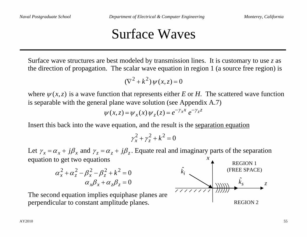
Surface Waves

Surface wave structures are best modeled by transmission lines. It is customary to use z as the direction of propagation. The scalar wave equation in region 1 (a source free region) is

2 2( ) ( , ) 0k x zψ∇ + =

where ( , )x zψ is a wave function that represents either E or H. The scattered wave function is separable with the general plane wave solution (see Appendix A.7)

( , ) ( ) ( ) x zx zx zx z x z e eγ γψ ψ ψ − −= =

Insert this back into the wave equation, and the result is the separation equation

2 2 2 0x z kγ γ+ + =

Let x x xjγ α β= + and z z zjγ α β= + . Equate real and imaginary parts of the separation equation to get two equations

2 2 2 2 2 00

x z x z

x x z z

kα α β βα β α β

+ − − + =+ =

The second equation implies equiphase planes are perpendicular to constant amplitude planes.

ik

z

REGION 2

REGION 1(FREE SPACE)

ˆsk

x

AY2010 56


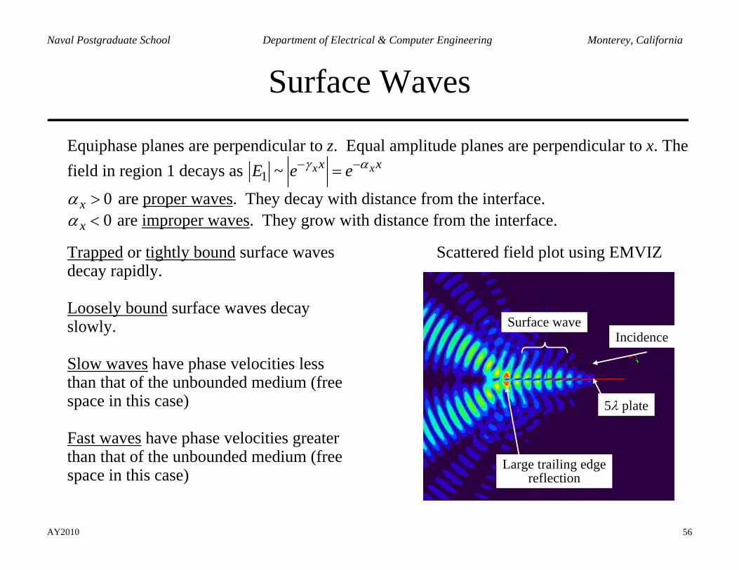
Surface Waves

Equiphase planes are perpendicular to z. Equal amplitude planes are perpendicular to x. The field in region 1 decays as 1 ~ x xx xE e eγ α− −=

0xα > are proper waves. They decay with distance from the interface. 0xα < are improper waves. They grow with distance from the interface.

Trapped or tightly bound surface waves decay rapidly. Loosely bound surface waves decay slowly. Slow waves have phase velocities less than that of the unbounded medium (free space in this case) Fast waves have phase velocities greater than that of the unbounded medium (free space in this case)

Scattered field plot using EMVIZ

5λ plate

Large trailing edgereflection

Surface waveIncidence

5λ plate

Large trailing edgereflection

Surface waveIncidence

AY2010 57


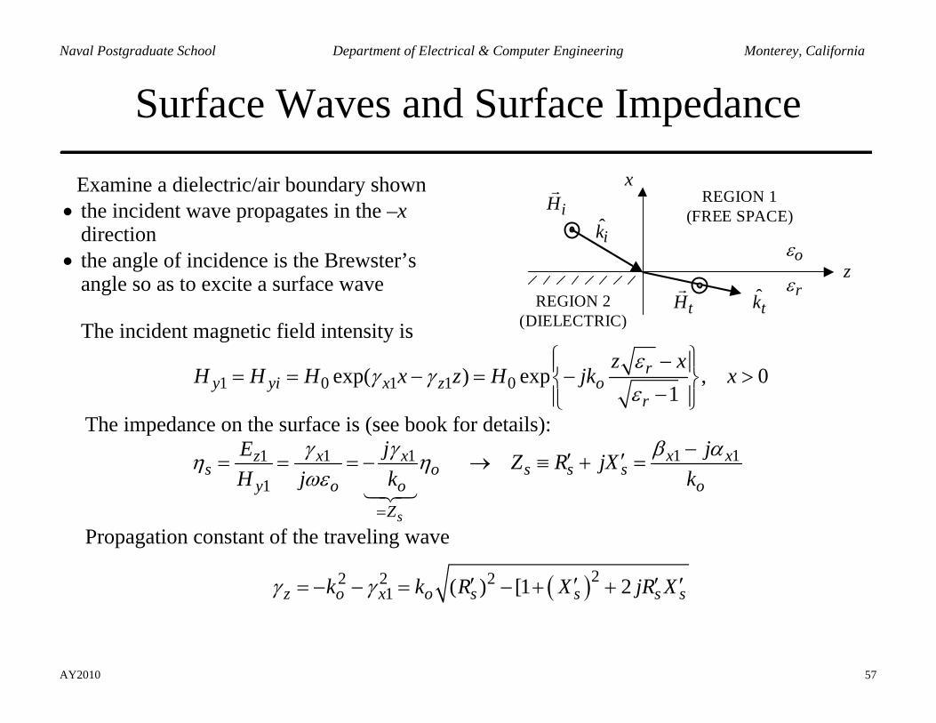
Surface Waves and Surface Impedance

Examine a dielectric/air boundary shown • the incident wave propagates in the –x

direction • the angle of incidence is the Brewster’s

angle so as to excite a surface wave The incident magnetic field intensity is

iH

ik

zREGION 2

(DIELECTRIC)

REGION 1(FREE SPACE)

tk

x

tHrε

oε

1 0 1 1 0exp( ) exp , 01

ry yi x z o

r

z xH H H x z H jk x

εγ γ

ε

⎧ ⎫−⎪ ⎪= = − = − >⎨ ⎬−⎪ ⎪⎩ ⎭

The impedance on the surface is (see book for details): 1 11

1

s

x xzs o

y o oZ

jEH j k

γ γη ηωε

=

= = = − 1 1x xs s s

o

jZ R jXk

β α−′ ′→ ≡ + =

Propagation constant of the traveling wave

( )22 2 21 ( ) [1 2z o x o s s s sk k R X jR Xγ γ ′ ′ ′ ′= − − = − + +

AY2010 58


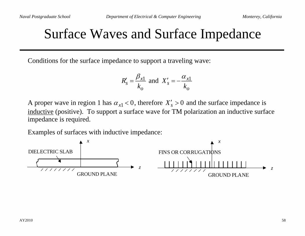
Surface Waves and Surface Impedance

Conditions for the surface impedance to support a traveling wave:

1 1 and x xs s

o oR X

k kβ α′ ′= = −

A proper wave in region 1 has 1 0xα < , therefore 0sX ′ > and the surface impedance is inductive (positive). To support a surface wave for TM polarization an inductive surface impedance is required. Examples of surfaces with inductive impedance:

x

zGROUND PLANE

DIELECTRIC SLAB

x

zGROUND PLANE

FINS OR CORRUGATIONS

AY2010 59


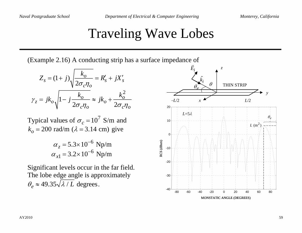
Traveling Wave Lobes

(Example 2.16) A conducting strip has a surface impedance of

(1 )2

os s s

c o

kZ j R jXσ η

′ ′= + = +

21

2 2o o

z o oc o c o

k kjk j jkγσ η σ η

= − ≈ +

Typical values of 710 S/mcσ = and 200 rad/m ( 3.14 cm)ok λ= = give

6

61

5.3 10 Np/m3.2 10 Np/m

z

x

αα

−

−= ×= ×

Significant levels occur in the far field. The lobe edge angle is approximately

49.35 / degreese Lθ λ≈ .

x

z

THIN STRIP

y

iE

ikθ

eθ

−L/2 L/2

-80 -60 -40 -20 0 20 40 60 80-40

-30

-20

-10

0

10

20

2 (m )L

RC

S (d

Bsm

)

MONSTATIC ANGLE (DEGREES)

eθL=5λ

-80 -60 -40 -20 0 20 40 60 80-40

-30

-20

-10

0

10

20

2 (m )L

RC

S (d

Bsm

)

MONSTATIC ANGLE (DEGREES)

eθL=5λ

Documents

Basic Theorems and Concepts - Naval Postgraduate Schoolfaculty.nps.edu/jenn/EC4630/TheoremsandConceptsV2.pdf · Naval Postgraduate School Department of Electrical & Computer Engineering