Embed Size (px)
Citation preview

Basic Probability and Statistics
CIS 8590 – Fall 2008 NLP 1

Outline
• Basic concepts in probability theory• Bayes’ rule• Random variable and distributions
Definition of Probability• Experiment: toss a coin twice• Sample space: possible outcomes of an experiment
– S = {HH, HT, TH, TT}• Event: a subset of possible outcomes
– A={HH}, B={HT, TH}• Probability of an event : a number assigned to an event
Pr(A)– Axiom 1: Pr(A) 0– Axiom 2: Pr(S) = 1– Axiom 3: For every sequence of disjoint events
– Example: Pr(A) = n(A)/N: frequentist statisticsPr( ) Pr( )i iii
A A
Joint Probability
• For events A and B, joint probability Pr(A,B) stands for the probability that both events happen.
• Example: A={HH}, B={HT, TH}, what is the joint probability Pr(A,B)?
Independence
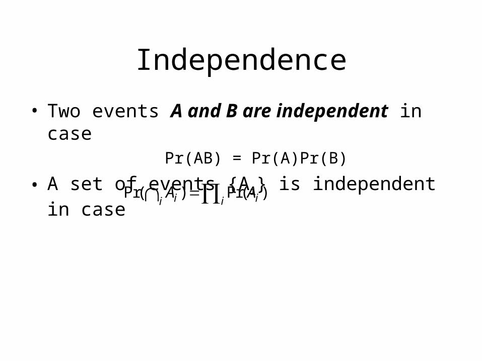
• Two events A and B are independent in casePr(AB) = Pr(A)Pr(B)
• A set of events {Ai} is independent in case
Pr( ) Pr( )i iiiA A
Independence
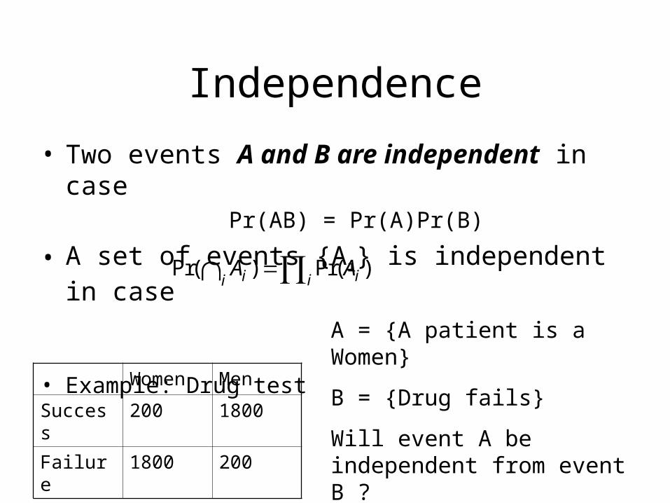
• Two events A and B are independent in casePr(AB) = Pr(A)Pr(B)
• A set of events {Ai} is independent in case
• Example: Drug test
Pr( ) Pr( )i iiiA A
Women Men
Success 200 1800
Failure 1800 200
A = {A patient is a Women}
B = {Drug fails}
Will event A be independent from event B ?
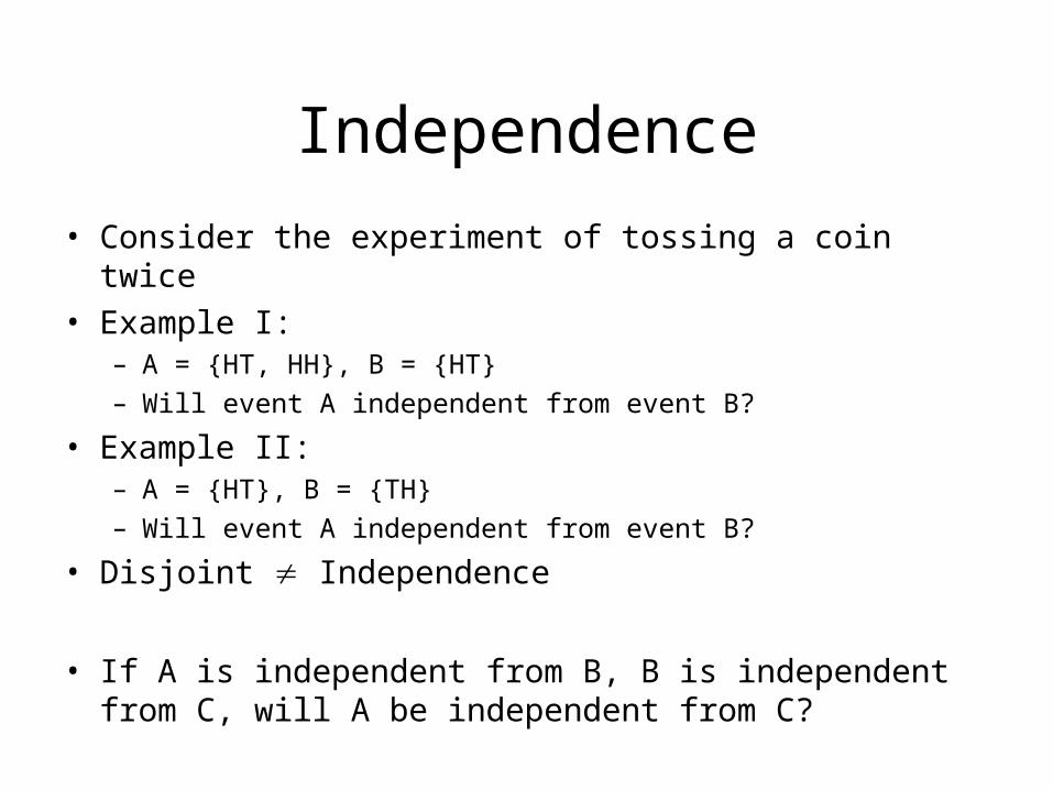
Independence• Consider the experiment of tossing a coin twice• Example I:
– A = {HT, HH}, B = {HT}– Will event A independent from event B?
• Example II:– A = {HT}, B = {TH}– Will event A independent from event B?
• Disjoint Independence
• If A is independent from B, B is independent from C, will A be independent from C?

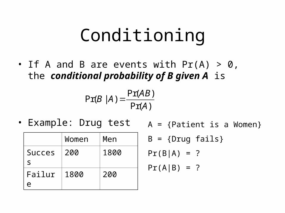
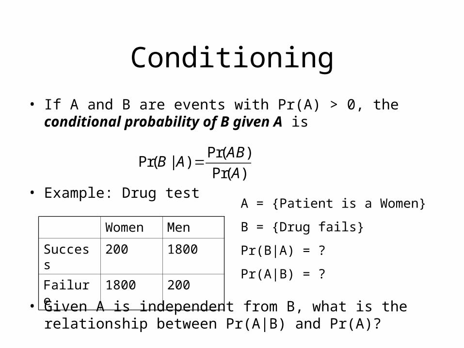
• If A and B are events with Pr(A) > 0, the conditional probability of B given A is
Conditioning
Pr( )Pr( | )
Pr( )
ABB A
A
• If A and B are events with Pr(A) > 0, the conditional probability of B given A is
• Example: Drug test
Conditioning
Pr( )Pr( | )
Pr( )
ABB A
A
Women Men
Success 200 1800
Failure 1800 200
A = {Patient is a Women}
B = {Drug fails}
Pr(B|A) = ?
Pr(A|B) = ?
• If A and B are events with Pr(A) > 0, the conditional probability of B given A is
• Example: Drug test
• Given A is independent from B, what is the relationship between Pr(A|B) and Pr(A)?
Conditioning
Pr( )Pr( | )
Pr( )
ABB A
A
Women Men
Success 200 1800
Failure 1800 200
A = {Patient is a Women}
B = {Drug fails}
Pr(B|A) = ?
Pr(A|B) = ?
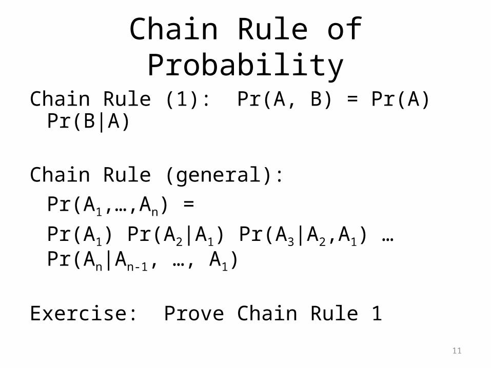
Chain Rule of Probability
Chain Rule (1): Pr(A, B) = Pr(A) Pr(B|A)
Chain Rule (general): Pr(A1,…,An) = Pr(A1) Pr(A2|A1) Pr(A3|A2,A1) … Pr(An|An-1, …, A1)
Exercise: Prove Chain Rule 1
11
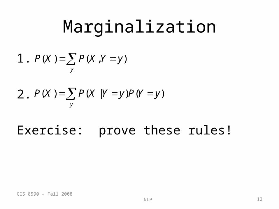
Marginalization
1.
2.
Exercise: prove these rules!
CIS 8590 – Fall 2008 NLP 12
y
yYXPXP ),()(
y
yYPyYXPXP )()|()(
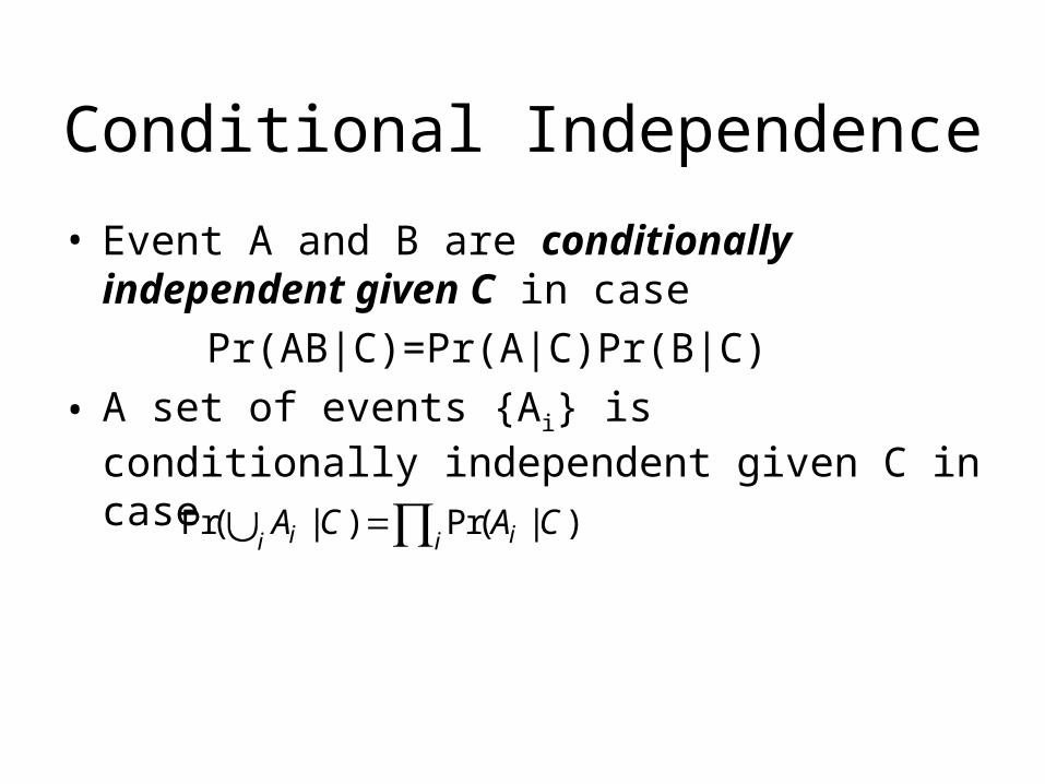
Conditional Independence
• Event A and B are conditionally independent given C in case
Pr(AB|C)=Pr(A|C)Pr(B|C)• A set of events {Ai} is conditionally independent given
C in casePr( | ) Pr( | )i iii
A C A C
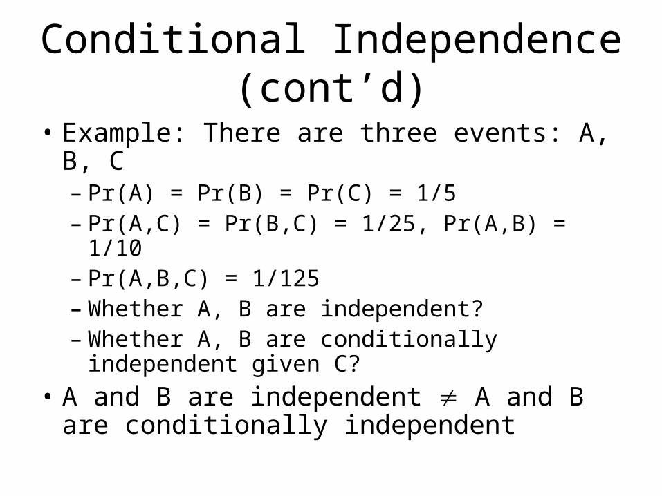
Conditional Independence (cont’d)
• Example: There are three events: A, B, C– Pr(A) = Pr(B) = Pr(C) = 1/5– Pr(A,C) = Pr(B,C) = 1/25, Pr(A,B) = 1/10– Pr(A,B,C) = 1/125– Whether A, B are independent?– Whether A, B are conditionally independent given
C?• A and B are independent A and B are
conditionally independent
Outline
• Important concepts in probability theory• Bayes’ rule• Random variables and distributions
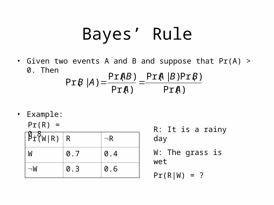
• Given two events A and B and suppose that Pr(A) > 0. Then
• Example:
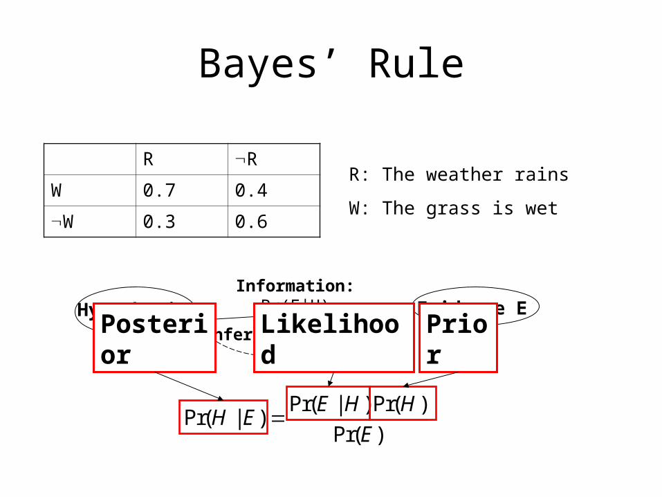
Bayes’ Rule
Pr(W|R) R R
W 0.7 0.4
W 0.3 0.6
R: It is a rainy day
W: The grass is wet
Pr(R|W) = ?
Pr(R) = 0.8
)Pr(
)Pr()|Pr(
)Pr(
)Pr()|Pr(
A
BBA
A
ABAB
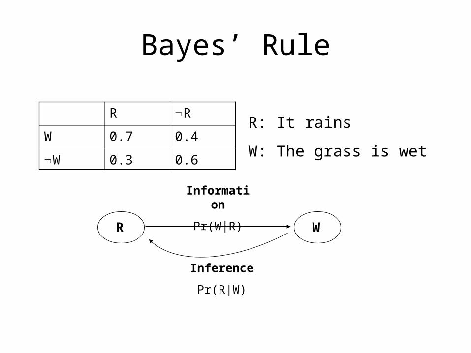
Bayes’ Rule
R R
W 0.7 0.4
W 0.3 0.6
R: It rains
W: The grass is wet
R W
Information
Pr(W|R)
Inference
Pr(R|W)
Pr( | ) Pr( )Pr( | )
Pr( )
E H HH E
E
Bayes’ Rule
R R
W 0.7 0.4
W 0.3 0.6
R: The weather rains
W: The grass is wet
Hypothesis H Evidence EInformation: Pr(E|H)
Inference: Pr(H|E) PriorLikelihoodPosterior
Outline
• Important concepts in probability theory• Bayes’ rule• Random variable and probability distribution
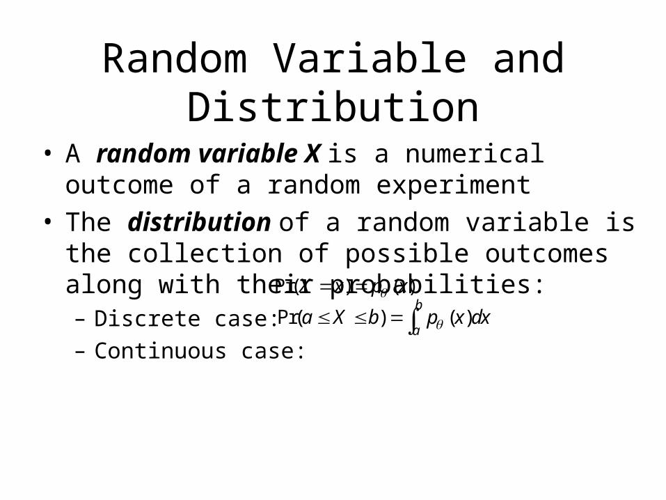
Random Variable and Distribution
• A random variable X is a numerical outcome of a random experiment
• The distribution of a random variable is the collection of possible outcomes along with their probabilities: – Discrete case:– Continuous case:
Pr( ) ( )X x p x
Pr( ) ( )b
aa X b p x dx
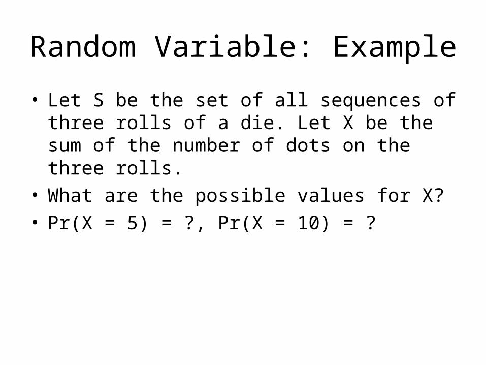
Random Variable: Example
• Let S be the set of all sequences of three rolls of a die. Let X be the sum of the number of dots on the three rolls.
• What are the possible values for X?• Pr(X = 5) = ?, Pr(X = 10) = ?
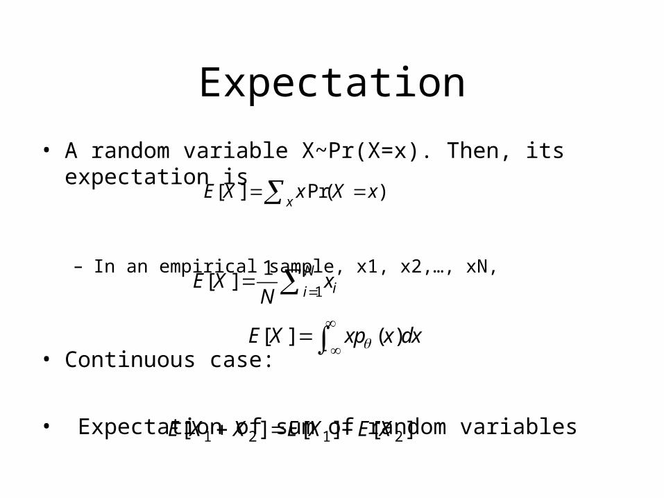
Expectation• A random variable X~Pr(X=x). Then, its expectation is
– In an empirical sample, x1, x2,…, xN,
• Continuous case:
• Expectation of sum of random variables
[ ] Pr( )x
E X x X x
1
1[ ]
Nii
E X xN
[ ] ( )E X xp x dx
1 2 1 2[ ] [ ] [ ]E X X E X E X
Expectation: Example
• Let S be the set of all sequence of three rolls of a die. Let X be the sum of the number of dots on the three rolls.
• What is E(X)?
• Let S be the set of all sequence of three rolls of a die. Let X be the product of the number of dots on the three rolls.
• What is E(X)?
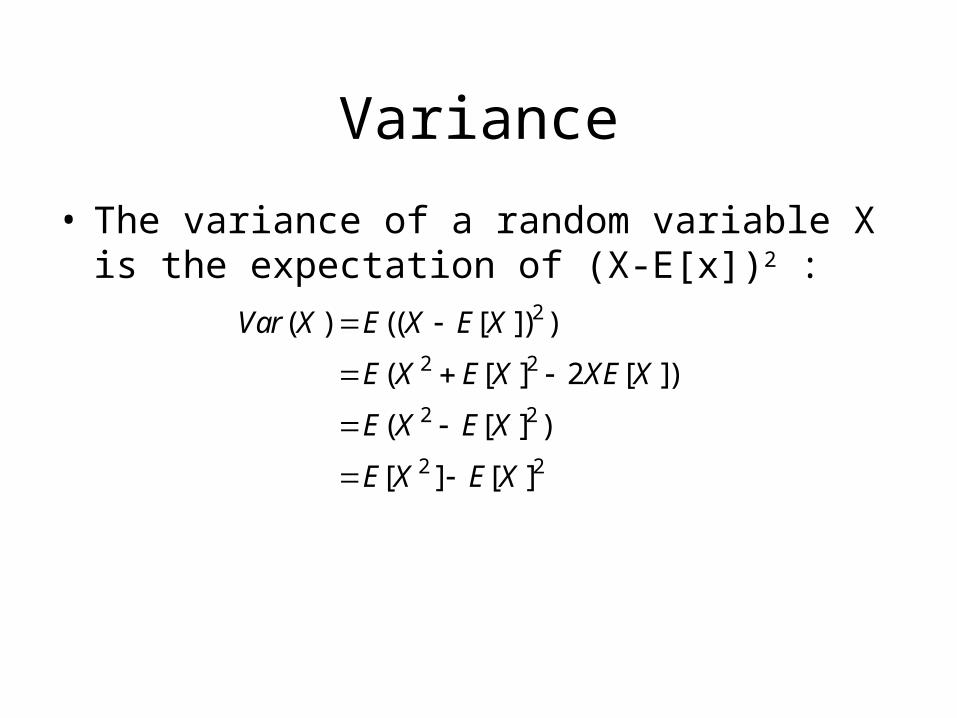
Variance
• The variance of a random variable X is the expectation of (X-E[x])2 :
2
2 2
2 2
2 2
( ) (( [ ]) )
( [ ] 2 [ ])
( [ ] )
[ ] [ ]
Var X E X E X
E X E X XE X
E X E X
E X E X
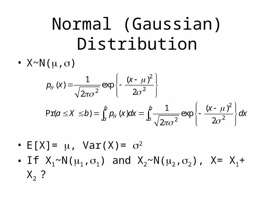
Normal (Gaussian) Distribution
• X~N(,)
• E[X]= , Var(X)= 2
• If X1~N(1,1) and X2~N(2,2), X= X1+ X2 ?
2
22
2
22
1 ( )( ) exp
22
1 ( )Pr( ) ( ) exp
22
b b
a a
xp x
xa X b p x dx dx
Sequence Labeling
Outline
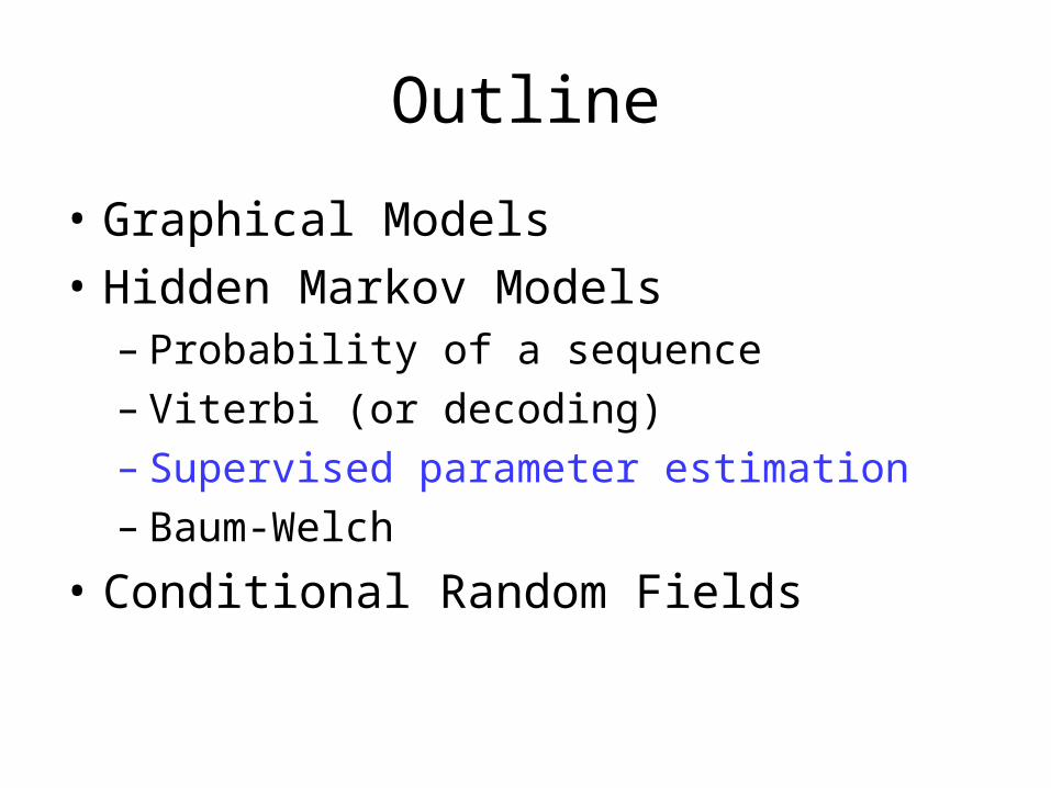
• Graphical Models• Hidden Markov Models– Probability of a sequence– Viterbi (or decoding)– Baum-Welch
• Conditional Random Fields
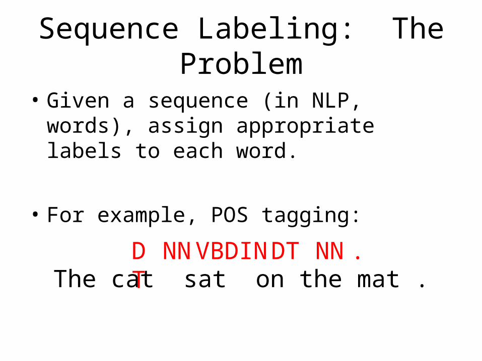
Sequence Labeling: The Problem
• Given a sequence (in NLP, words), assign appropriate labels to each word.
• For example, POS tagging:
The cat sat on the mat .DT NN VBD IN DT NN .
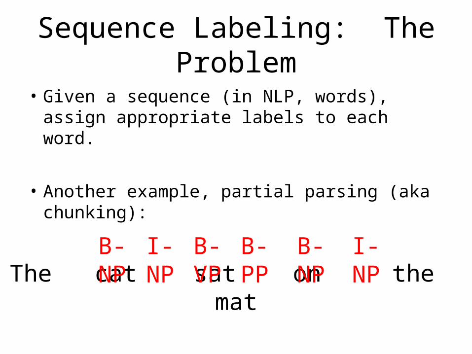
Sequence Labeling: The Problem
• Given a sequence (in NLP, words), assign appropriate labels to each word.
• Another example, partial parsing (aka chunking):
The cat sat on the matB-NP I-NP B-VPB-PP B-NP I-NP
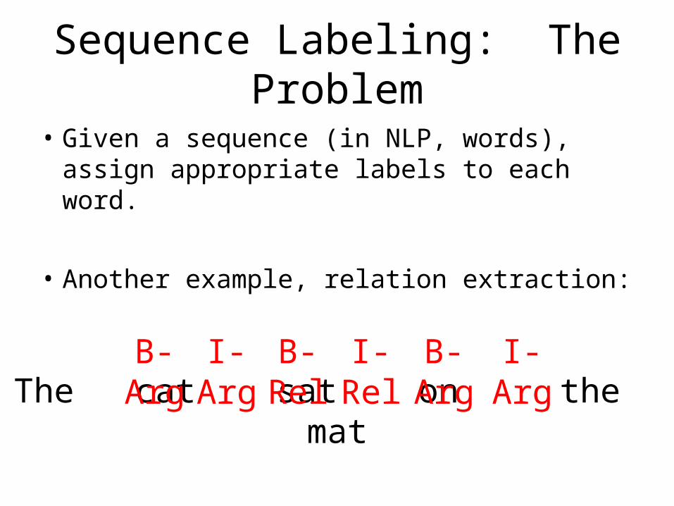
Sequence Labeling: The Problem
• Given a sequence (in NLP, words), assign appropriate labels to each word.
• Another example, relation extraction:
The cat sat on the matB-ArgI-ArgB-Rel I-Rel B-Arg I-Arg
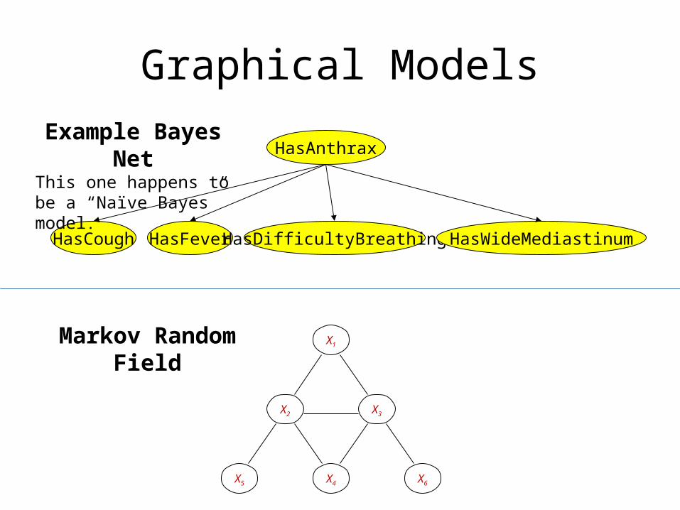
Graphical Models
HasAnthrax
HasCough HasFever HasDifficultyBreathing HasWideMediastinum
X1
X3X2
X4 X6X5
Example Bayes NetThis one happens to be a “Naïve Bayes” model.
Markov Random Field
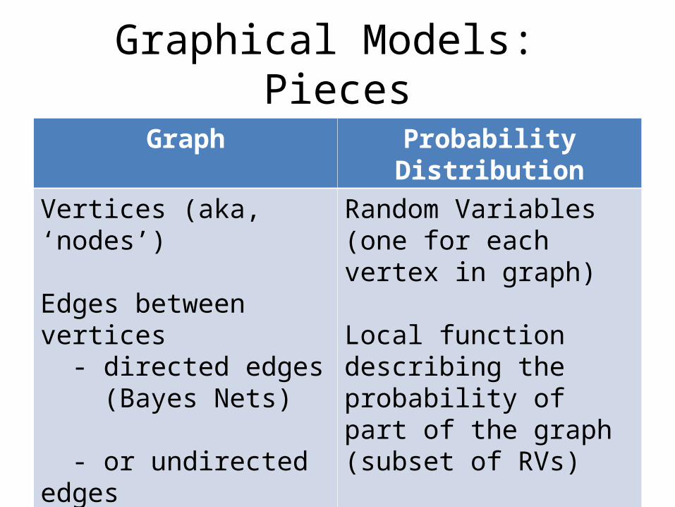
Graphical Models: Pieces
Graph Probability DistributionVertices (aka, ‘nodes’)
Edges between vertices - directed edges (Bayes Nets)
- or undirected edges (Markov Random Fields)
Random Variables (one for each vertex in graph)
Local function describing the probability of part of the graph (subset of RVs)
A formula for combining local functions into an overall probability
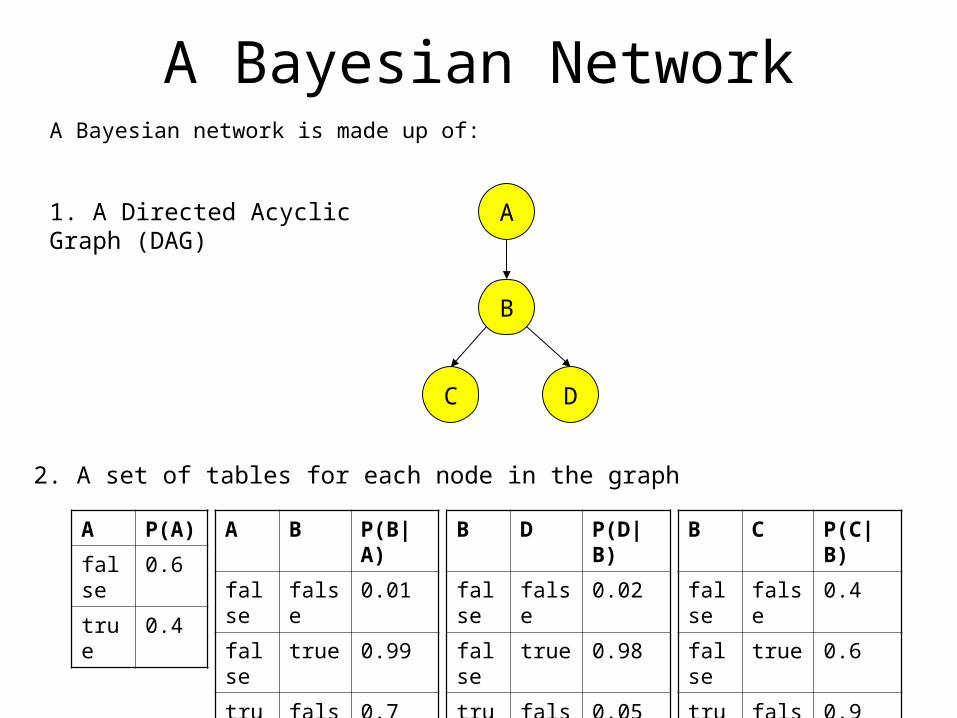
A Bayesian NetworkA Bayesian network is made up of:
A P(A)
false 0.6
true 0.4
A
B
C D
A B P(B|A)
false false 0.01
false true 0.99
true false 0.7
true true 0.3
B C P(C|B)
false false 0.4
false true 0.6
true false 0.9
true true 0.1
B D P(D|B)
false false 0.02
false true 0.98
true false 0.05
true true 0.95
1. A Directed Acyclic Graph (DAG)
2. A set of tables for each node in the graph
Weng-Keen Wong, Oregon State University ©2005 34
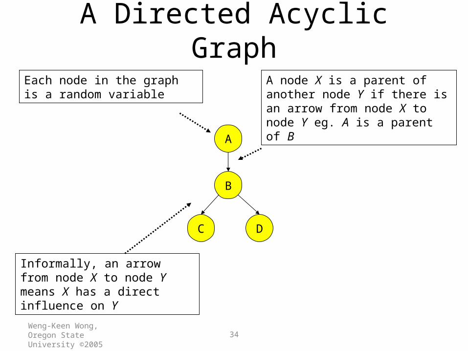
A Directed Acyclic Graph
A
B
C D
Each node in the graph is a random variable
A node X is a parent of another node Y if there is an arrow from node X to node Y eg. A is a parent of B
Informally, an arrow from node X to node Y means X has a direct influence on Y

A Set of Tables for Each NodeEach node Xi has a conditional probability distribution P(Xi | Parents(Xi)) that quantifies the effect of the parents on the node
The parameters are the probabilities in these conditional probability tables (CPTs)
A P(A)
false 0.6
true 0.4
A B P(B|A)
false false 0.01
false true 0.99
true false 0.7
true true 0.3
B C P(C|B)
false false 0.4
false true 0.6
true false 0.9
true true 0.1
B D P(D|B)
false false 0.02
false true 0.98
true false 0.05
true true 0.95
A
B
C D
Weng-Keen Wong, Oregon State University ©2005 36
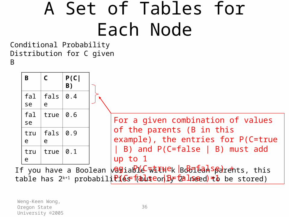
A Set of Tables for Each NodeConditional Probability Distribution for C given B
If you have a Boolean variable with k Boolean parents, this table has 2k+1 probabilities (but only 2k need to be stored)
B C P(C|B)
false false 0.4
false true 0.6
true false 0.9
true true 0.1 For a given combination of values of the parents (B in this example), the entries for P(C=true | B) and P(C=false | B) must add up to 1 eg. P(C=true | B=false) + P(C=false |B=false )=1
Weng-Keen Wong, Oregon State University ©2005 37
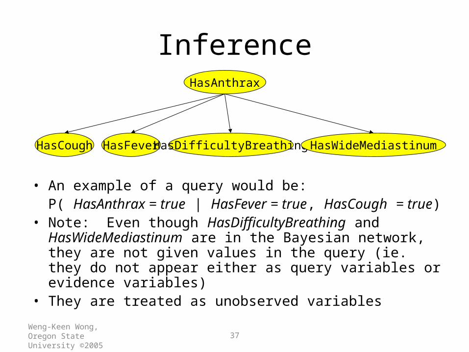
Inference
• An example of a query would be:P( HasAnthrax = true | HasFever = true, HasCough = true)
• Note: Even though HasDifficultyBreathing and HasWideMediastinum are in the Bayesian network, they are not given values in the query (ie. they do not appear either as query variables or evidence variables)
• They are treated as unobserved variables
HasAnthrax
HasCough HasFever HasDifficultyBreathing HasWideMediastinum
Weng-Keen Wong, Oregon State University ©2005 38
The Bad News
• Exact inference is feasible in small to medium-sized networks
• Exact inference in large networks takes a very long time
• We resort to approximate inference techniques which are much faster and give pretty good results

An Example
R It rains
W The grass is wet
U People bring umbrella
Pr(UW|R)=Pr(U|R)Pr(W|R)
Pr(UW| R)=Pr(U| R)Pr(W| R)
R
W U
Pr(W|R) R R
W 0.7 0.4
W 0.3 0.6
Pr(U|R) R R
U 0.9 0.2
U 0.1 0.8
Pr(U|W) = ?
Pr(R) = 0.8

An Example
R It rains
W The grass is wet
U People bring umbrella
Pr(UW|R)=Pr(U|R)Pr(W|R)
Pr(UW| R)=Pr(U| R)Pr(W| R)
R
W U
Pr(W|R) R R
W 0.7 0.4
W 0.3 0.6
Pr(U|R) R R
U 0.9 0.2
U 0.1 0.8
Pr(U|W) = ?
Pr(R) = 0.8

An Example
R It rains
W The grass is wet
U People bring umbrella
Pr(UW|R)=Pr(U|R)Pr(W|R)
Pr(UW| R)=Pr(U| R)Pr(W| R)
R
W U
Pr(W|R) R R
W 0.7 0.4
W 0.3 0.6
Pr(U|R) R R
U 0.9 0.2
U 0.1 0.8
Pr(U|W) = ?
Pr(R) = 0.8
Outline
• Graphical Models• Hidden Markov Models– Probability of a sequence (decoding)– Viterbi (Best hidden layer sequence)– Supervised parameter estimation– Baum-Welch
• Conditional Random Fields
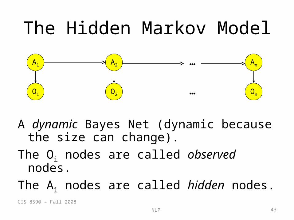
The Hidden Markov Model
A dynamic Bayes Net (dynamic because the size can change).
The Oi nodes are called observed nodes.The Ai nodes are called hidden nodes.CIS 8590 – Fall 2008
NLP 43
A1
O1
A2
O2
An
On…
…
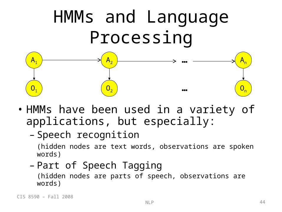
HMMs and Language Processing
• HMMs have been used in a variety of applications, but especially:– Speech recognition
(hidden nodes are text words, observations are spoken words)
– Part of Speech Tagging(hidden nodes are parts of speech, observations are words)
CIS 8590 – Fall 2008 NLP 44
A1
O1
A2
O2
An
On…
…

HMM Independence Assumptions
HMMs assume that:• Ai is independent of A1 through Ai-2, given Ai-1
• Oi is independent of all other nodes, given Ai
• P(Ai | Ai-1) and P(Oi | Ai) do not depend on I
Not very realistic assumptions about language – but HMMs are often good enough, and very convenient.
CIS 8590 – Fall 2008 NLP 45
A1
O1
A2
O2
An
On…
…
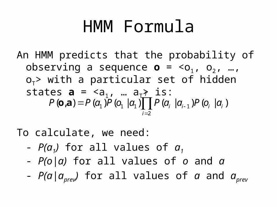
HMM Formula
An HMM predicts that the probability of observing a sequence o = <o1, o2, …, oT> with a particular set of hidden states a = <a1, … aT> is:
To calculate, we need: - P(a1) for all values of a1
- P(o|a) for all values of o and a- P(a|aprev) for all values of a and aprev
T
iiiii aoPaaPaoPaPP
21111 )|()|()|()(),( ao

HMM: Pieces1) A set of states S = {s1, …, sN} that are the values which hidden nodes
may take.
2) A vocabulary, or set of states V = {v1, …, vM} that are the values which an observed node may take.
3) Initial probabilities P(si) for all i- Written as a vector of N initial probabilities, called π
4) Transition probabilities P(sj | si) for all j, I- Written as an NxN ‘transition matrix’ A
5) Observation probabilities P(vj|si) for all j, i- written as an MxN ‘observation matrix’ B
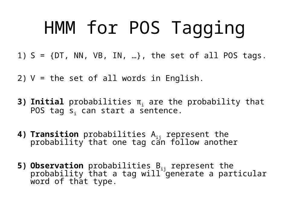
HMM for POS Tagging1) S = {DT, NN, VB, IN, …}, the set of all POS tags.
2) V = the set of all words in English.
3) Initial probabilities πi are the probability that POS tag si can start a sentence.
4) Transition probabilities Aij represent the probability that one tag can follow another
5) Observation probabilities Bij represent the probability that a tag will generate a particular word of that type.
Outline
• Graphical Models• Hidden Markov Models– Probability of a sequence– Viterbi (or decoding)– Supervised parameter estimation– Baum-Welch
• Conditional Random Fields
What’s the probability of a sentence?
Suppose I asked you, ‘What’s the probability of seeing a sentence w1, …, wT on the web?’
If we have an HMM model of English, we can use it to estimate the probability.
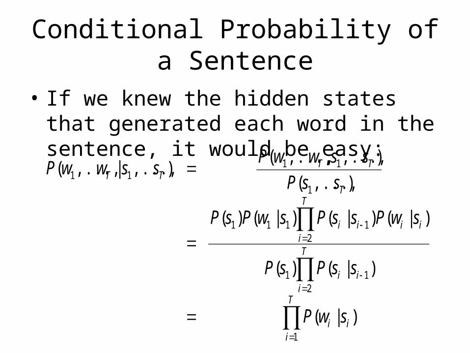
Conditional Probability of a Sentence
• If we knew the hidden states that generated each word in the sentence, it would be easy:
T
iii
T
iii
T
iiiii
T
TTTT
swP
ssPsP
swPssPswPsP
ssP
sswwPsswwP
1
211
21111
1
1111
)|(
)|()(
)|()|()|()(
),...,(
),...,,,...,(),...,|,...,(
Probability of a Sentence
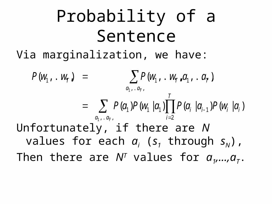
Via marginalization, we have:
Unfortunately, if there are N values for each ai (s1 through sN),
Then there are NT values for a1,…,aT.
T
T
aa
T
iiiii
aaTTT
awPaaPawPaP
aawwPwwP
,..., 21111
,...,111
1
1
)|()|()|()(
),...,,,...,(),...,(
)|,...()( 1 ixooPt tti
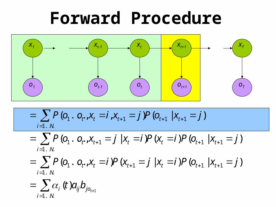
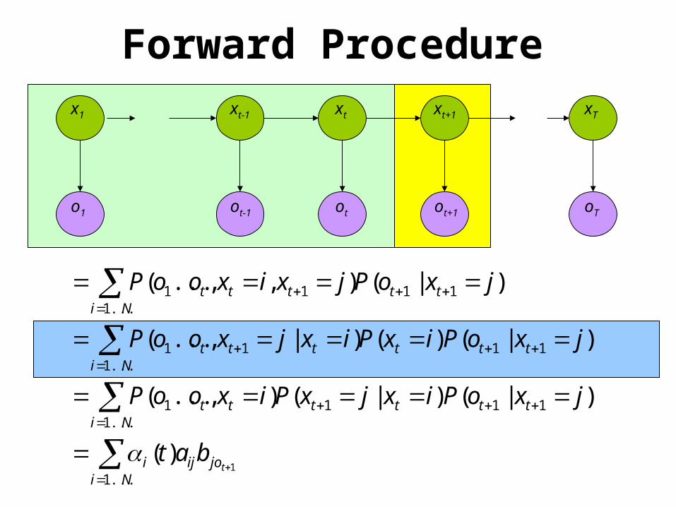
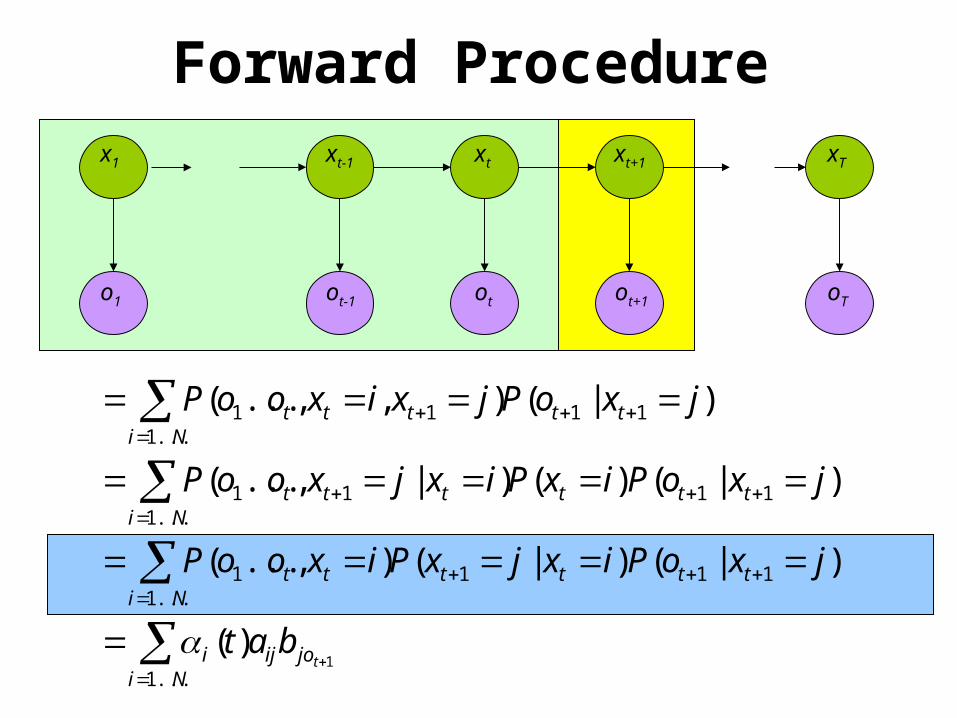
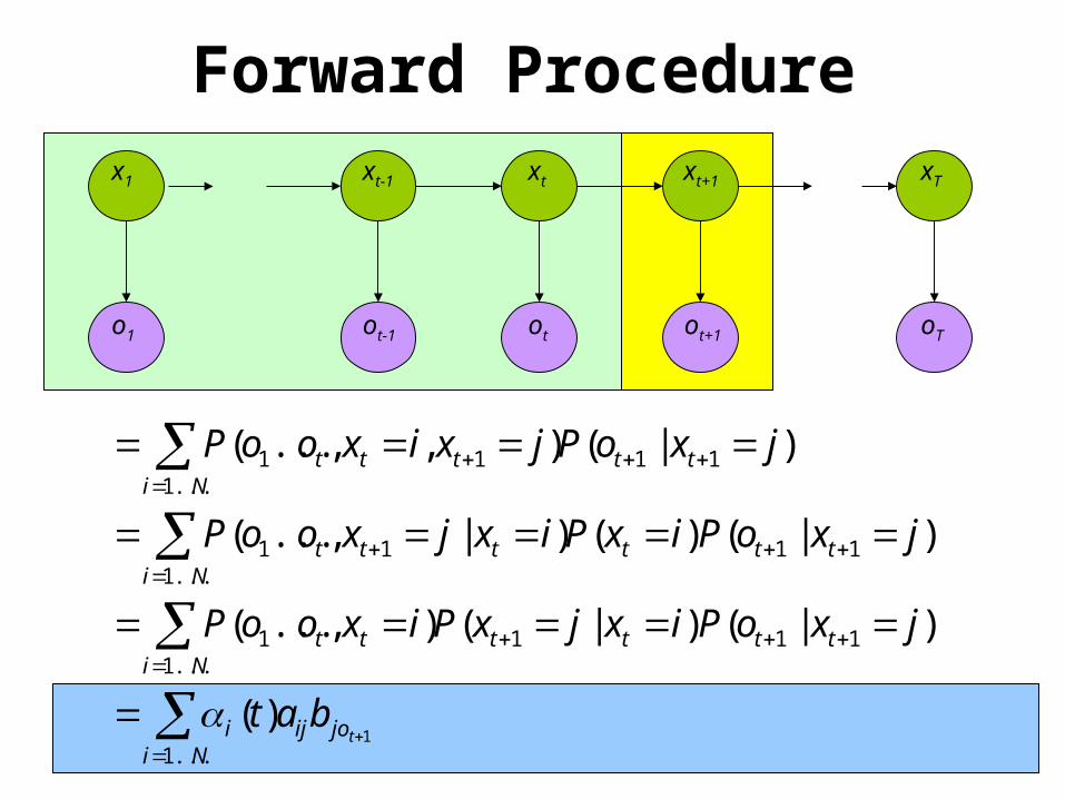
Forward Procedure
oTo1 otot-1 ot+1
x1 xt+1 xTxtxt-1
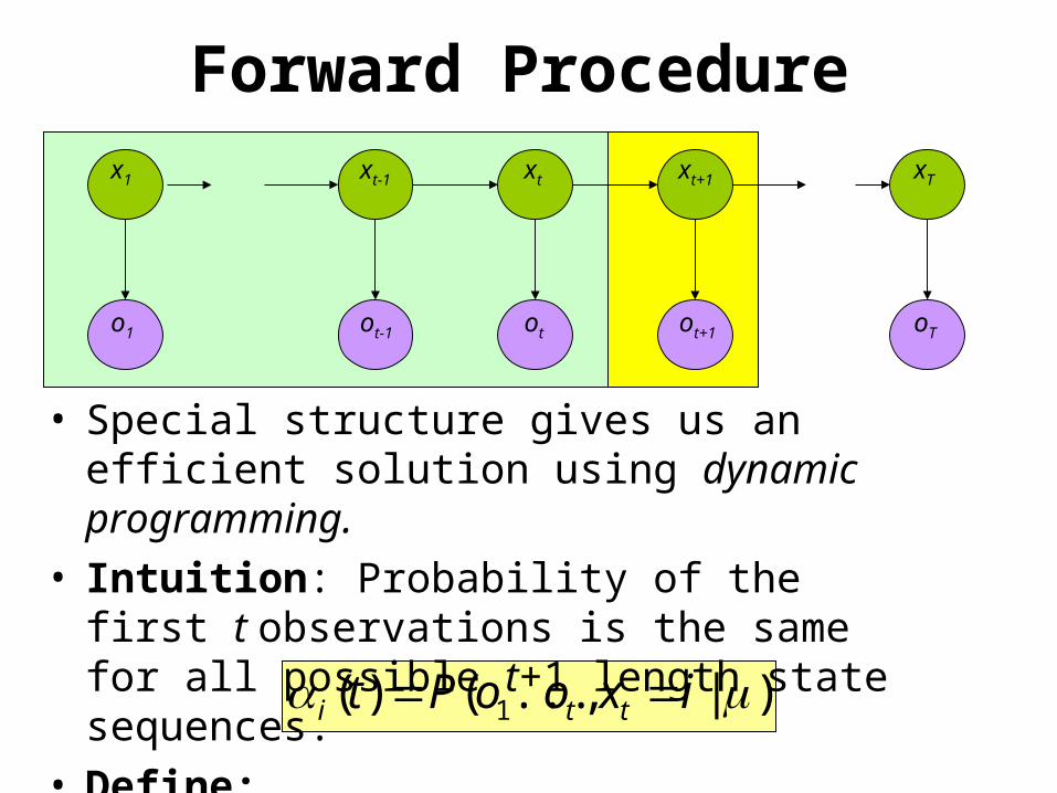
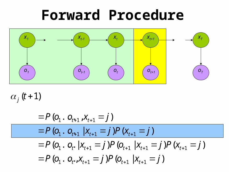
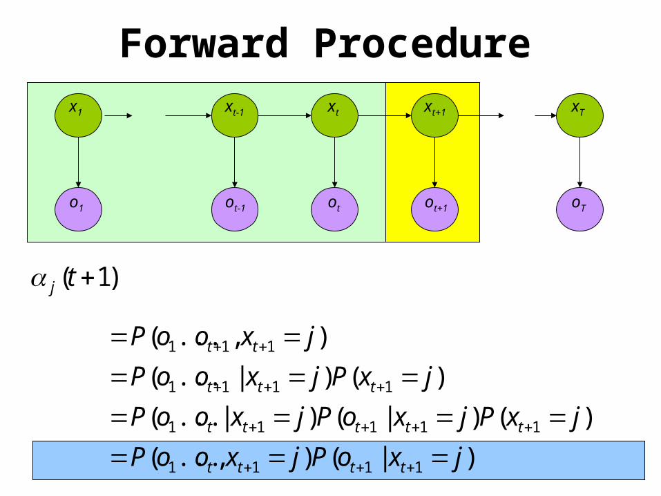
• Special structure gives us an efficient solution using dynamic programming.
• Intuition: Probability of the first t observations is the same for all possible t+1 length state sequences.
• Define:

)|(),...(
)()|()|...(
)()|...(
),...(
1111
11111
1111
111
jxoPjxooP
jxPjxoPjxooP
jxPjxooP
jxooP
tttt
ttttt
ttt
tt
oTo1 otot-1 ot+1
x1 xt+1 xTxtxt-1
Forward Procedure
)1( tj
oTo1 otot-1 ot+1
x1 xt+1 xTxtxt-1
Forward Procedure
)1( tj
)|(),...(
)()|()|...(
)()|...(
),...(
1111
11111
1111
111
jxoPjxooP
jxPjxoPjxooP
jxPjxooP
jxooP
tttt
ttttt
ttt
tt

oTo1 otot-1 ot+1
x1 xt+1 xTxtxt-1
Forward Procedure
)1( tj
)|(),...(
)()|()|...(
)()|...(
),...(
1111
11111
1111
111
jxoPjxooP
jxPjxoPjxooP
jxPjxooP
jxooP
tttt
ttttt
ttt
tt
oTo1 otot-1 ot+1
x1 xt+1 xTxtxt-1
Forward Procedure
)1( tj
)|(),...(
)()|()|...(
)()|...(
),...(
1111
11111
1111
111
jxoPjxooP
jxPjxoPjxooP
jxPjxooP
jxooP
tttt
ttttt
ttt
tt
Nijoiji
ttttNi
tt
tttNi
ttt
ttNi
ttt
tbat
jxoPixjxPixooP
jxoPixPixjxooP
jxoPjxixooP
...1
111...1
1
11...1
11
11...1
11
1)(
)|()|(),...(
)|()()|,...(
)|(),,...(
oTo1 otot-1 ot+1
x1 xt+1 xTxtxt-1
Forward Procedure
Nijoiji
ttttNi
tt
tttNi
ttt
ttNi
ttt
tbat
jxoPixjxPixooP
jxoPixPixjxooP
jxoPjxixooP
...1
111...1
1
11...1
11
11...1
11
1)(
)|()|(),...(
)|()()|,...(
)|(),,...(
oTo1 otot-1 ot+1
x1 xt+1 xTxtxt-1
Forward Procedure
Nijoiji
ttttNi
tt
tttNi
ttt
ttNi
ttt
tbat
jxoPixjxPixooP
jxoPixPixjxooP
jxoPjxixooP
...1
111...1
1
11...1
11
11...1
11
1)(
)|()|(),...(
)|()()|,...(
)|(),,...(
oTo1 otot-1 ot+1
x1 xt+1 xTxtxt-1
Forward Procedure
Nijoiji
ttttNi
tt
tttNi
ttt
ttNi
ttt
tbat
jxoPixjxPixooP
jxoPixPixjxooP
jxoPjxixooP
...1
111...1
1
11...1
11
11...1
11
1)(
)|()|(),...(
)|()()|,...(
)|(),,...(
oTo1 otot-1 ot+1
x1 xt+1 xTxtxt-1
Forward Procedure

)|...()( ixooPt tTti
oTo1 otot-1 ot+1
x1 xt+1 xTxtxt-1
Backward Procedure
1)1( Ti
Nj
jioiji tbatt
...1
)1()(
Probability of the rest of the states given the first state

oTo1 otot-1 ot+1
x1 xt+1 xTxtxt-1
Decoding Solution
N
ii TOP
1
)()|(
N
iiiOP
1
)1()|(
)()()|(1
ttOP i
N
ii
Forward Procedure
Backward Procedure
Combination

Outline
• Graphical Models• Hidden Markov Models– Probability of a sequence– Viterbi (or decoding)– Supervised parameter estimation– Baum-Welch
• Conditional Random Fields
oTo1 otot-1 ot+1
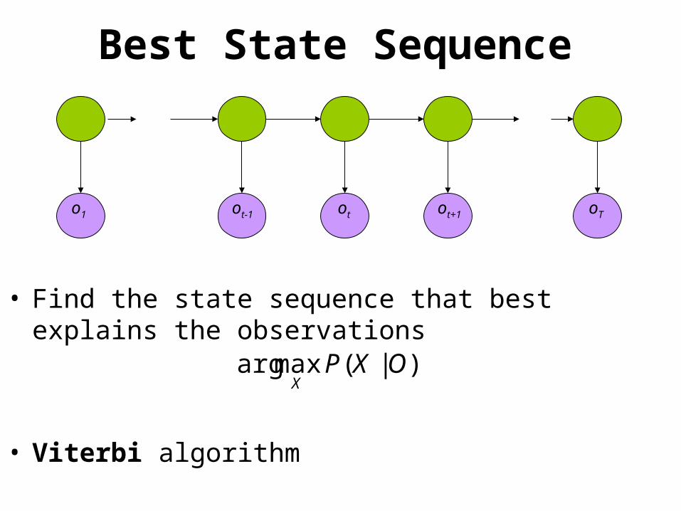
Best State Sequence
• Find the state sequence that best explains the observations
• Viterbi algorithm
)|(maxarg OXPX
oTo1 otot-1 ot+1
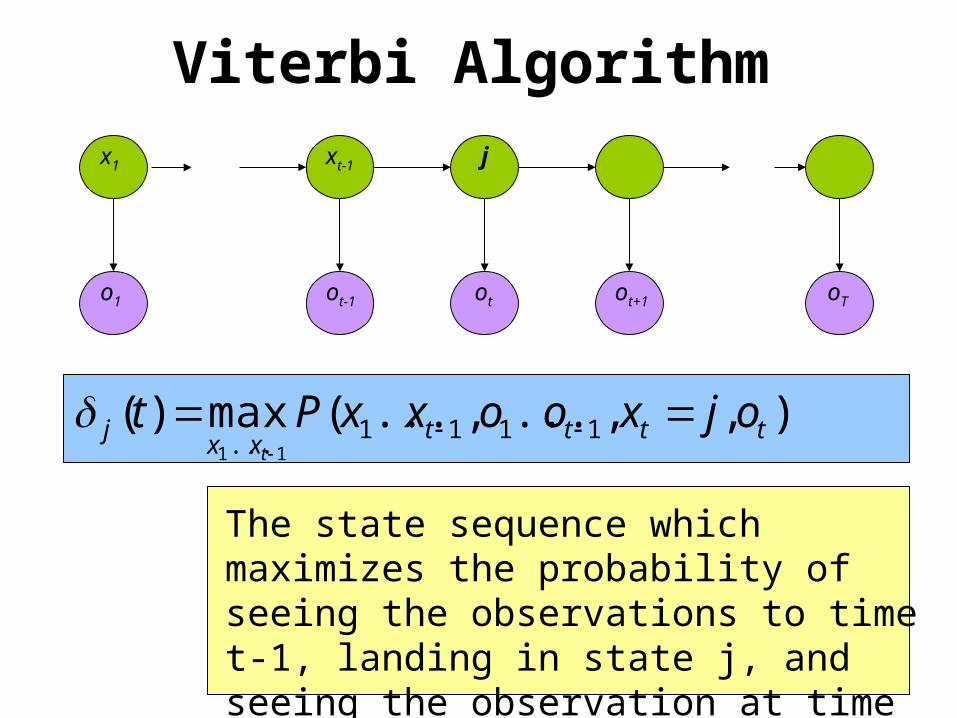
Viterbi Algorithm
),,...,...(max)( 1111... 11
ttttxx
j ojxooxxPtt
The state sequence which maximizes the probability of seeing the observations to time t-1, landing in state j, and seeing the observation at time t
x1 xt-1 j
oTo1 otot-1 ot+1
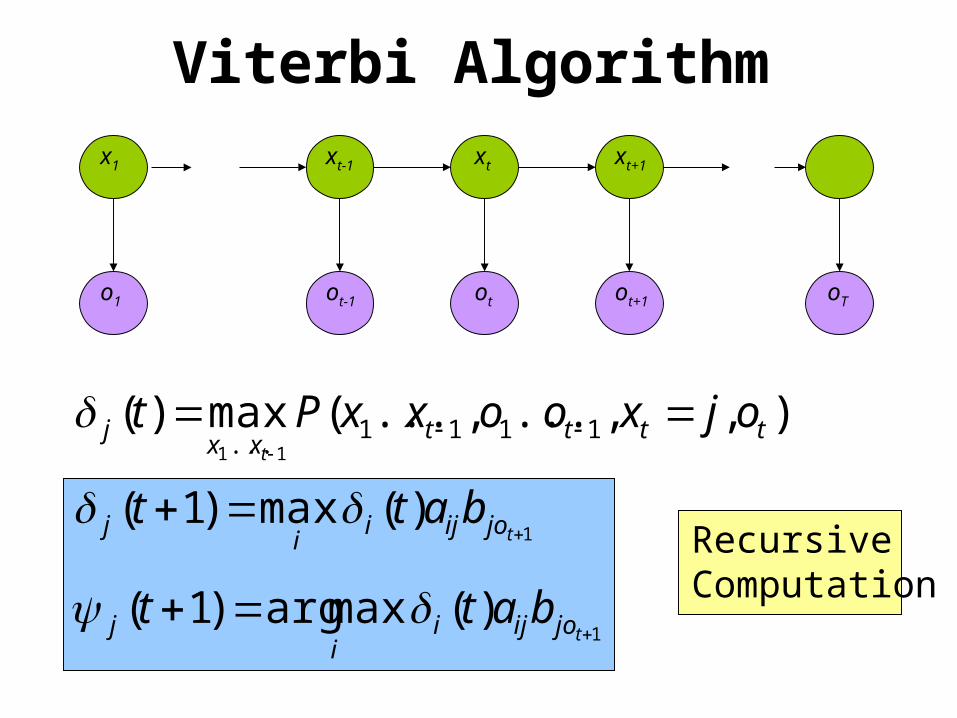
Viterbi Algorithm
),,...,...(max)( 1111... 11
ttttxx
j ojxooxxPtt
1)(max)1(
tjoijii
j batt
1)(maxarg)1(
tjoijii
j batt Recursive Computation
x1 xt-1 xt xt+1
oTo1 otot-1 ot+1
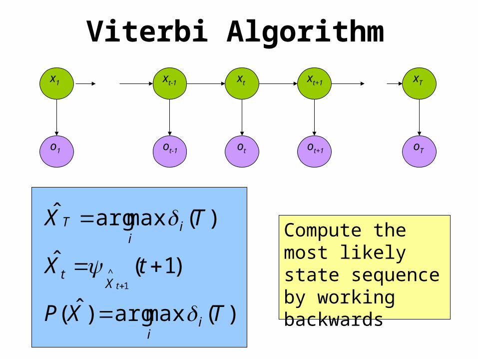
Viterbi Algorithm
)(maxargˆ TX ii
T
)1(ˆ1
^
tXtX
t
)(maxarg)ˆ( TXP ii
Compute the most likely state sequence by working backwards
x1 xt-1 xt xt+1 xT
Outline
• Graphical Models• Hidden Markov Models– Probability of a sequence– Viterbi (or decoding)– Supervised parameter estimation– Baum-Welch
• Conditional Random Fields

Supervised Parameter Estimation
• Given an observation sequence and states, find the HMM model (π, A, and B) that is most likely to produce the sequence.
• For example, POS-tagged data from the Penn Treebank
A
B
AAA
BBB B
oTo1 otot-1 ot+1
x1 xt-1 xt xt+1 xT
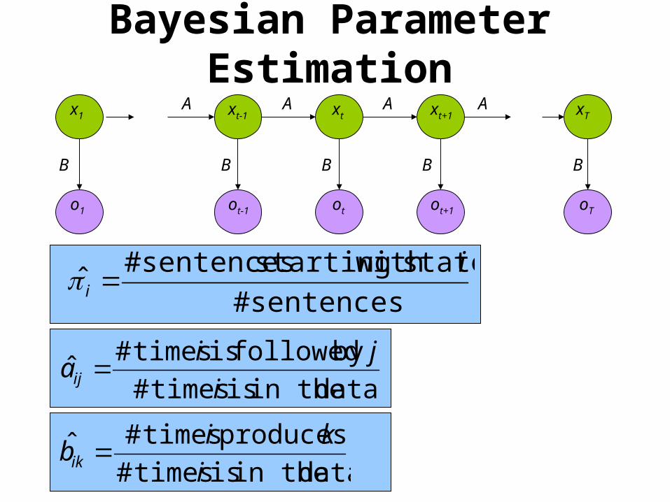
Bayesian Parameter EstimationA
B
AAA
BBB B
oTo1 otot-1 ot+1
x1 xt-1 xt xt+1 xT
sentences#
state with starting sentences#ˆ
ii
data in the is times#
by followed is times#ˆ
i
jiaij
data in the is times#
produces times#ˆi
kibik
Outline
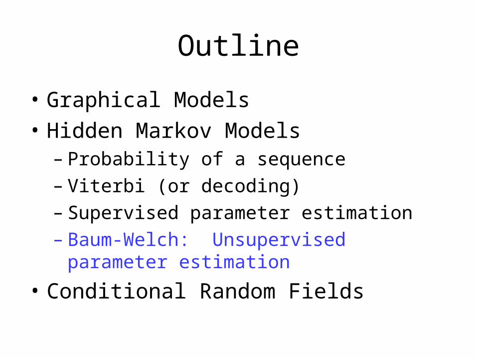
• Graphical Models• Hidden Markov Models– Probability of a sequence– Viterbi (or decoding)– Supervised parameter estimation– Baum-Welch: Unsupervised parameter
estimation
• Conditional Random Fields
oTo1 otot-1 ot+1
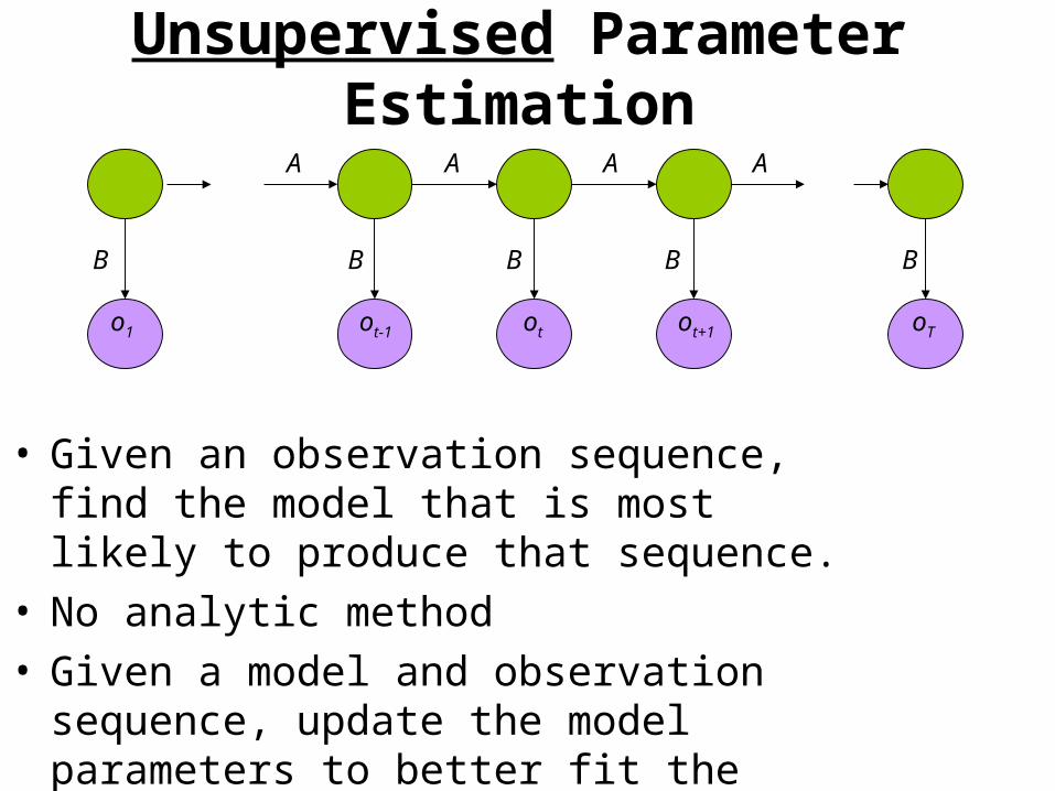
Unsupervised Parameter Estimation
• Given an observation sequence, find the model that is most likely to produce that sequence.
• No analytic method• Given a model and observation sequence, update
the model parameters to better fit the observations.
A
B
AAA
BBB B
oTo1 otot-1 ot+1
Parameter EstimationA
B
AAA
BBB B
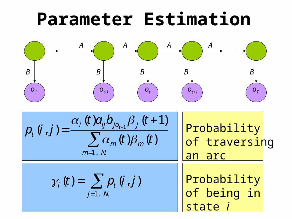
Nmmm
jjoijit tt
tbatjip t
...1
)()(
)1()(),( 1
Probability of traversing an arc
Njti jipt
...1
),()( Probability of being in state i
oTo1 otot-1 ot+1
Parameter EstimationA
B
AAA
BBB B
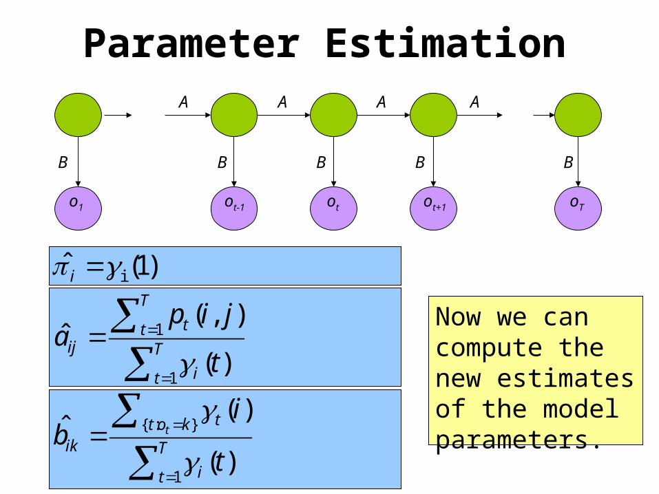
)1(ˆ i i
Now we can compute the new estimates of the model parameters.
T
t i
T
t tij
t
jipa
1
1
)(
),(ˆ
T
t i
kot t
ikt
ib t
1
}:{
)(
)(ˆ

oTo1 otot-1 ot+1
Parameter EstimationA
B
AAA
BBB B
• Guarantee: P(o1:T|A,B,π) <= P(o1:T|A ̂,B ̂, π� )• In other words, by repeating this procedure, we
can gradually improve how well the HMM fits the unlabeled data.
• There is no guarantee that this will converge to the best possible HMM, however.
oTo1 otot-1 ot+1
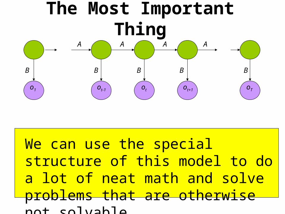
The Most Important ThingA
B
AAA
BBB B
We can use the special structure of this model to do a lot of neat math and solve problems that are otherwise not solvable.
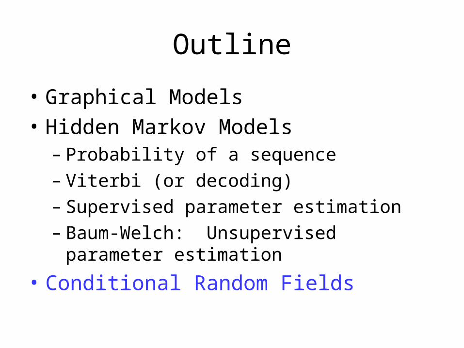
Outline
• Graphical Models• Hidden Markov Models– Probability of a sequence– Viterbi (or decoding)– Supervised parameter estimation– Baum-Welch: Unsupervised parameter
estimation
• Conditional Random Fields

Discriminative (Conditional) Models
• HMMs are called generative models:That is, if you want them to, they can tell you
P(sentence) by marginalizing over P(sentence, labels)
• Most often, though, people are most interested in the conditional probability P(labels | sentence)
• Discriminative (also called conditional) models directly represent P(labels | sentence)
• You can’t find out P(sentence) or P(sentence,labels)• But for P(labels | sentence), they tend to be more accurate
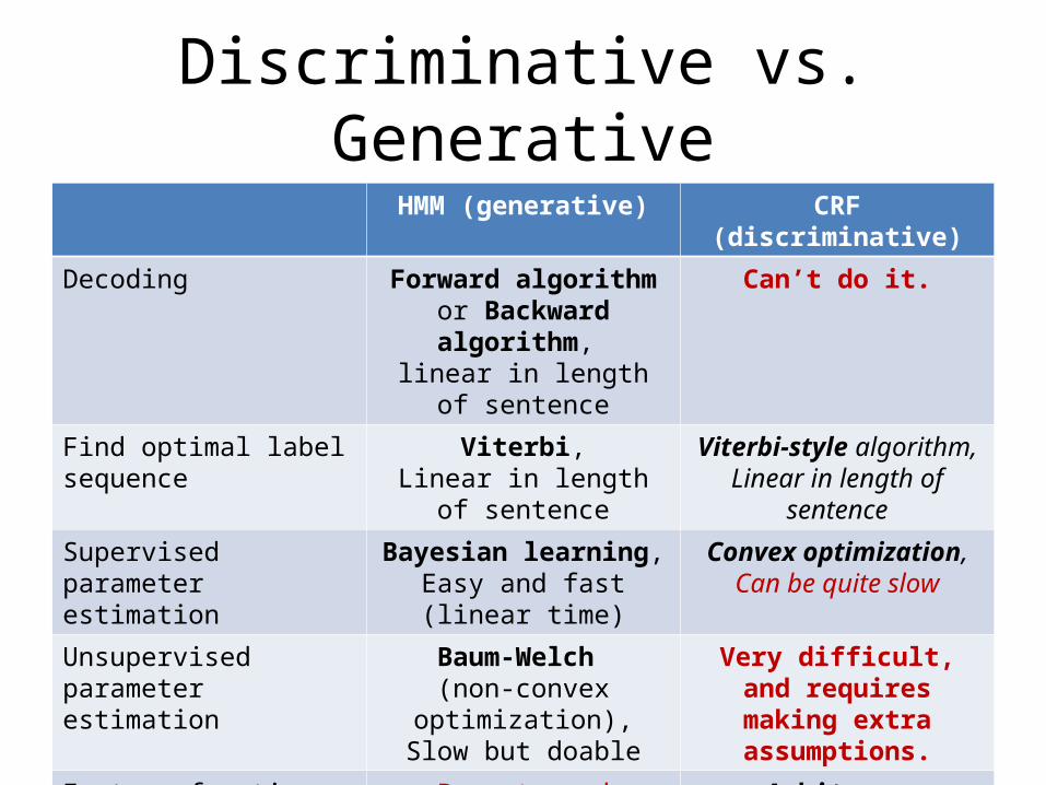
Discriminative vs. GenerativeHMM (generative) CRF (discriminative)
Decoding Forward algorithm or Backward algorithm,
linear in length of sentence
Can’t do it.
Find optimal label sequence
Viterbi,Linear in length of
sentence
Viterbi-style algorithm,Linear in length of sentence
Supervised parameter estimation
Bayesian learning,Easy and fast (linear time)
Convex optimization,Can be quite slow
Unsupervised parameter estimation
Baum-Welch (non-convex optimization),
Slow but doable
Very difficult, and requires making extra assumptions.
Feature functions Parents and children in the graph
Restrictive!
Arbitrary functions of a latent state and any
portion of the observed nodes
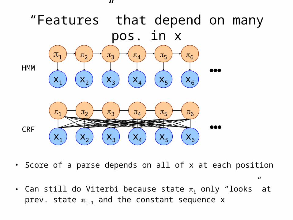
“Features” that depend on many pos. in x
• Score of a parse depends on all of x at each position
• Can still do Viterbi because state i only “looks” at prev. state i-1 and the constant sequence x
1
x1
2
x2
3
x3
4
x4
5
x5
6
x6
…
1
x1
2
x2
3
x3
4
x4
5
x5
6
x6
…
HMM
CRF
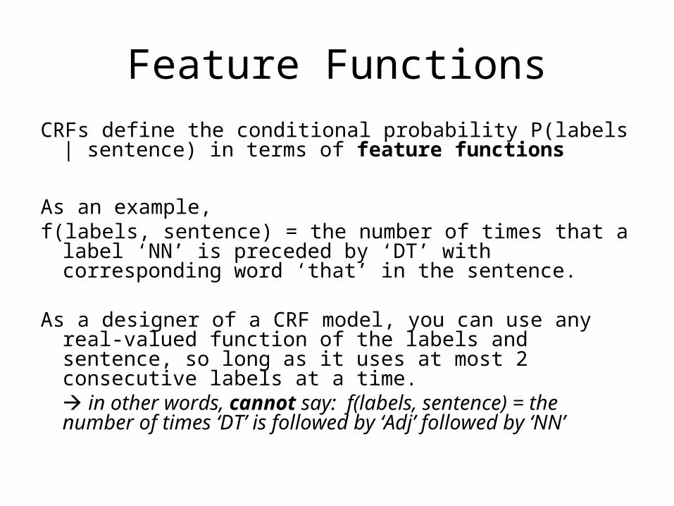
Feature FunctionsCRFs define the conditional probability P(labels | sentence) in
terms of feature functions
As an example, f(labels, sentence) = the number of times that a label ‘NN’ is
preceded by ‘DT’ with corresponding word ‘that’ in the sentence.
As a designer of a CRF model, you can use any real-valued function of the labels and sentence, so long as it uses at most 2 consecutive labels at a time. in other words, cannot say: f(labels, sentence) = the number of times ‘DT’ is followed by ‘Adj’ followed by ‘NN’
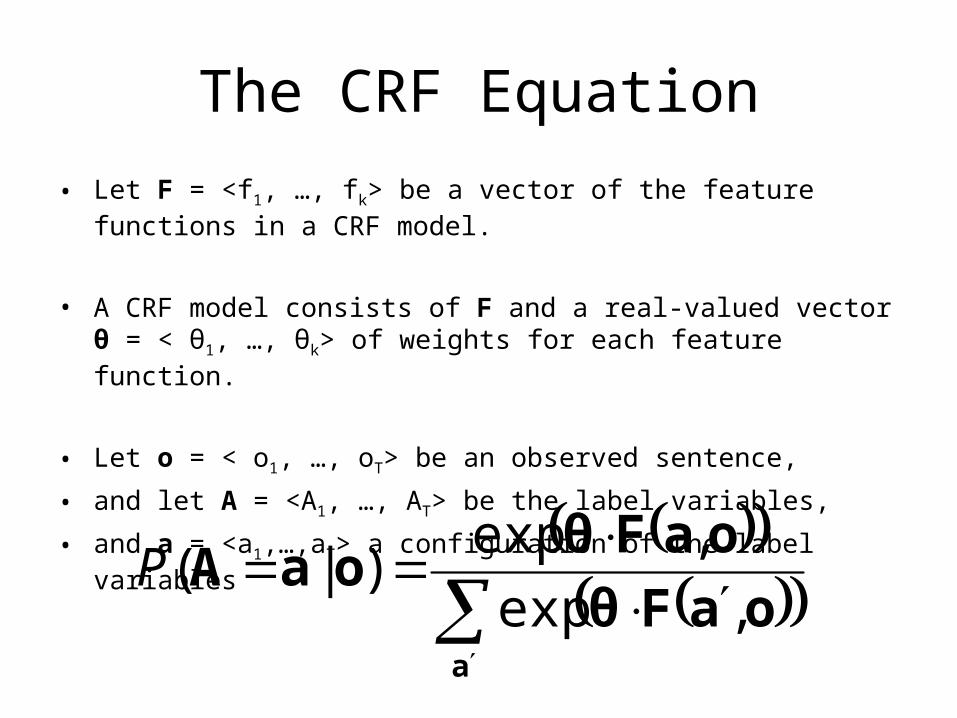
The CRF Equation• Let F = <f1, …, fk> be a vector of the feature functions in a CRF model.
• A CRF model consists of F and a real-valued vector θ = < θ1, …, θk> of weights for each feature function.
• Let o = < o1, …, oT> be an observed sentence,
• and let A = <A1, …, AT> be the label variables,
• and a = <a1,…,aT> a configuration of the label variables
a
oaFθ
oaFθoaA
,exp
,exp)|(P
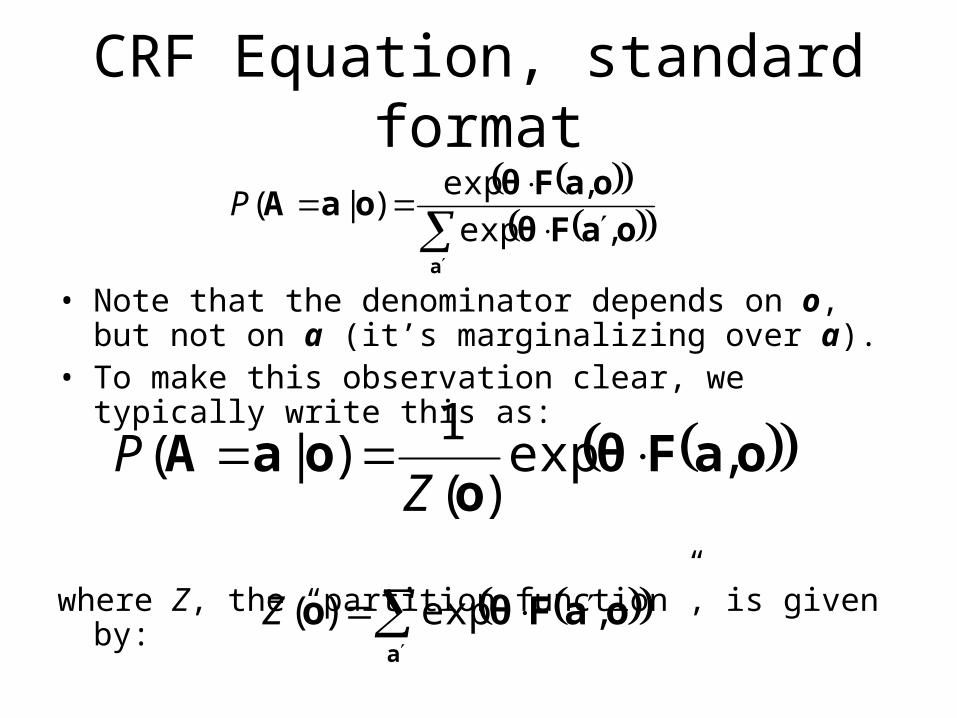
CRF Equation, standard format
• Note that the denominator depends on o, but not on a (it’s marginalizing over a).
• To make this observation clear, we typically write this as:
where Z, the “partition function”, is given by:
oaFθo
oaA ,exp)(
1)|( Z
P
a
oaFθo ,exp)(Z
a
oaFθ
oaFθoaA
,exp
,exp)|(P
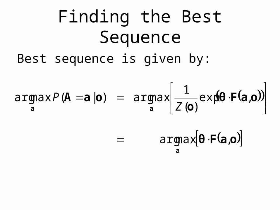
Finding the Best Sequence
Best sequence is given by:
oaFθ
oaFθo
oaA
a
aa
,maxarg
,exp)(
1maxarg)|(maxarg
ZP
oTo1 otot-1 ot+1
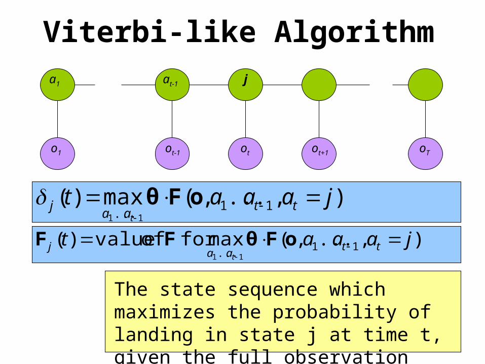
Viterbi-like Algorithm
),...,(max)( 11... 11
jaaat ttaa
jt
oFθ
The state sequence which maximizes the probability of landing in state j at time t, given the full observation sequence.
a1 at-1 j
),...,(maxfor of value)( 11... 11
jaaat ttaa
jt
oFθFF

oTo1 otot-1 ot+1
Viterbi-like Algorithma1 at-1 j
),,()(max)1( 1 jaiatt ttii
j oFFθ
),...,(max)( 11... 11
jaaat ttaa
jt
oFθ
),...,(maxfor of value)( 11... 11
jaaat ttaa
jt
oFθFF
),,()(maxarg)1( 1 jaiatt ttii
j oFFθ
oTo1 otot-1 ot+1
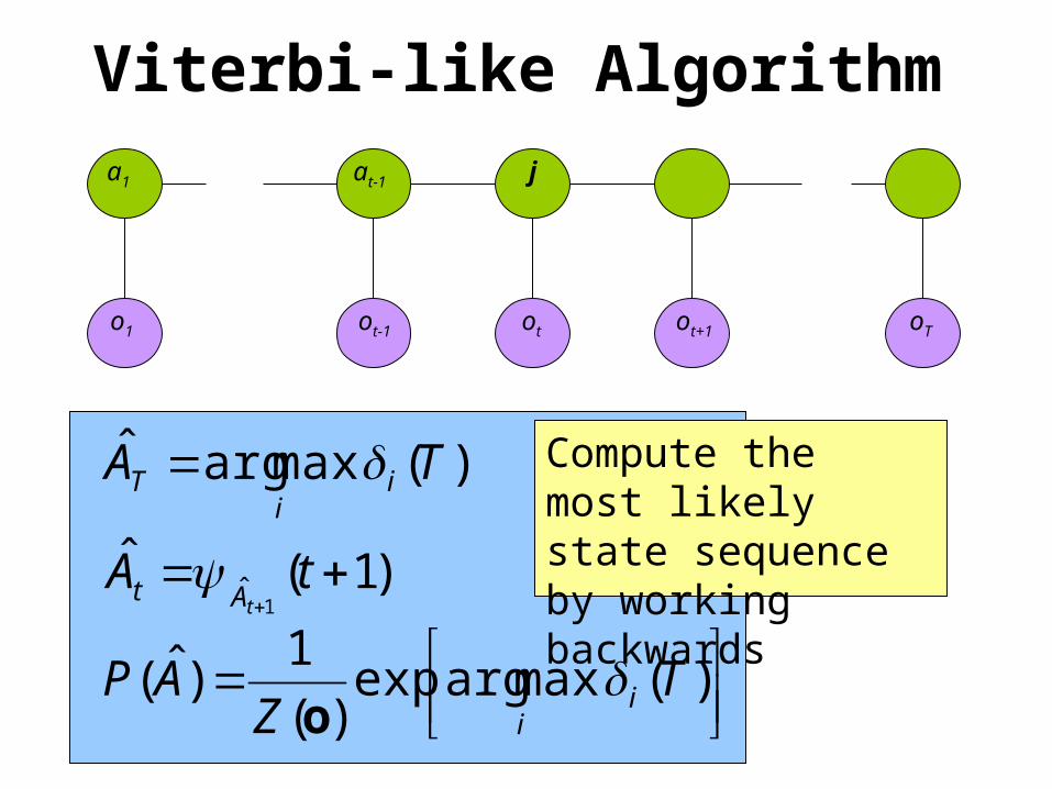
Viterbi-like Algorithma1 at-1 j
)(maxargˆ TA ii
T
)1(ˆ1
ˆ tA
tAt
)(maxargexp
)(
1)ˆ( TZ
AP ii
o
Compute the most likely state sequence by working backwards
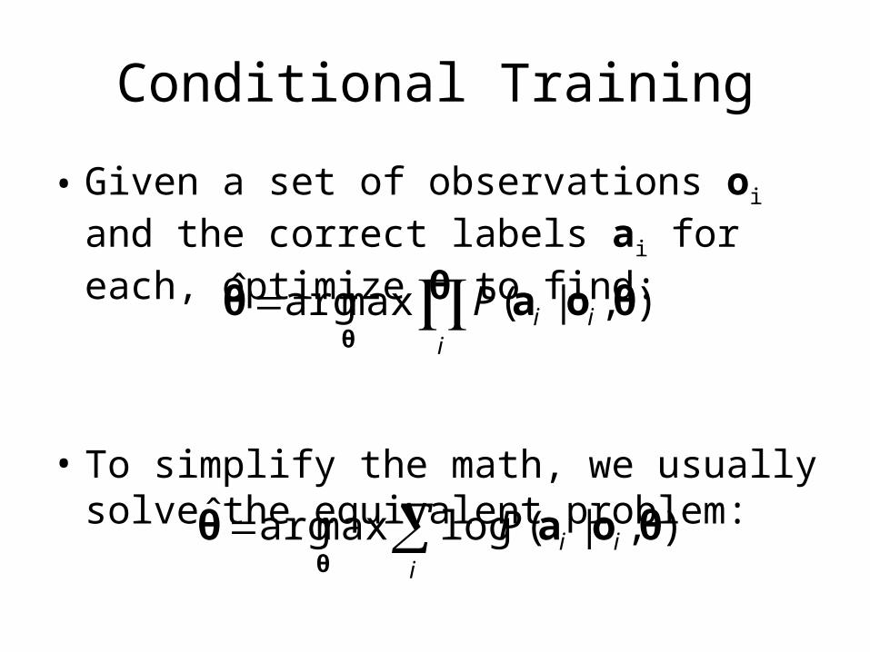
Conditional Training
• Given a set of observations oi and the correct labels ai for each, optimize θ to find:
• To simplify the math, we usually solve the equivalent problem:
i
iiP ),|(maxargˆ θoaθθ
i
iiP ),|(logmaxargˆ θoaθθ

Convex Optimization
• Like any function optimization task, we can optimize by taking the derivative and finding the roots.
• However, the roots are hard to find
• Instead, common practice is to use a numerical optimization procedure called “quasi-Newton optimization”.• In particular, the “Limited-memory Broyden-Fletcher-Goldfarb-Shanno”
(LBFGS) method is most popular.
• I won’t explain LBFGS, but I will explain what you need in order to use it.
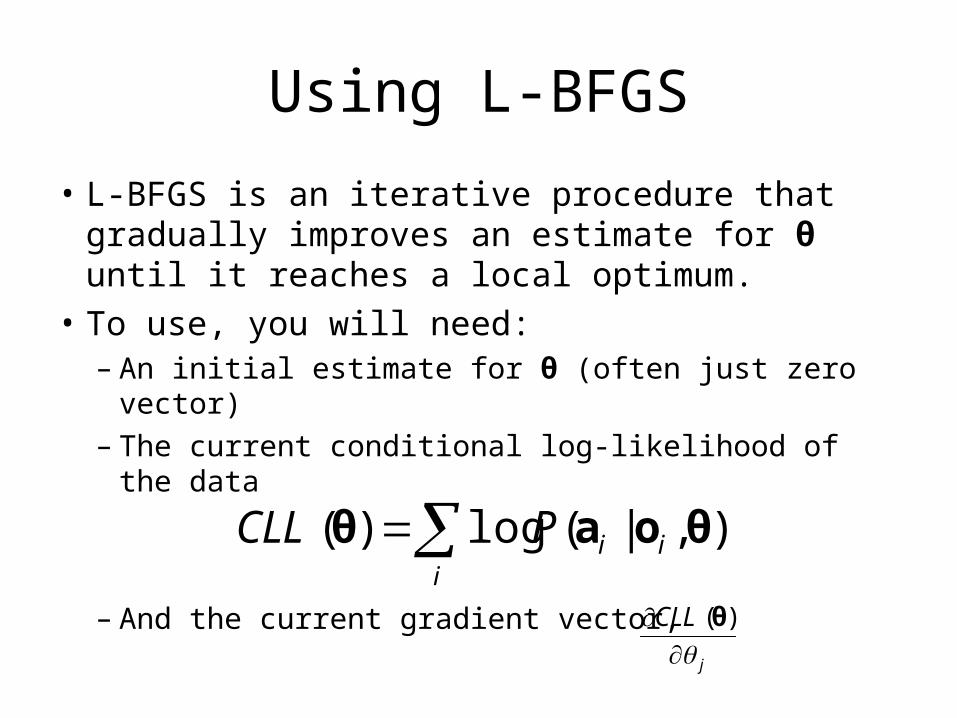
Using L-BFGS
• L-BFGS is an iterative procedure that gradually improves an estimate for θ until it reaches a local optimum.
• To use, you will need:– An initial estimate for θ (often just zero vector)– The current conditional log-likelihood of the data
– And the current gradient vector,
i
iiPCLL ),|(log)( θoaθ
j
CLL
)(θ
Using L-BFGS
Supply L-BFGS with these 3 things, and it will return an improved setting for θ.
Repeat as necessary, until the conditional log-likelihood doesn’t change much between iterations.
Since the negative log-likelihood is convex, this will converge to a global optimum (although it may take a while).
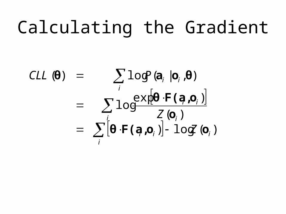
Calculating the Gradient
iiii
i i
ii
iii
ZZ
PCLL
)(log))(
)explog
),|(log)(
oo,F(aθo
o,F(aθ
θoaθ
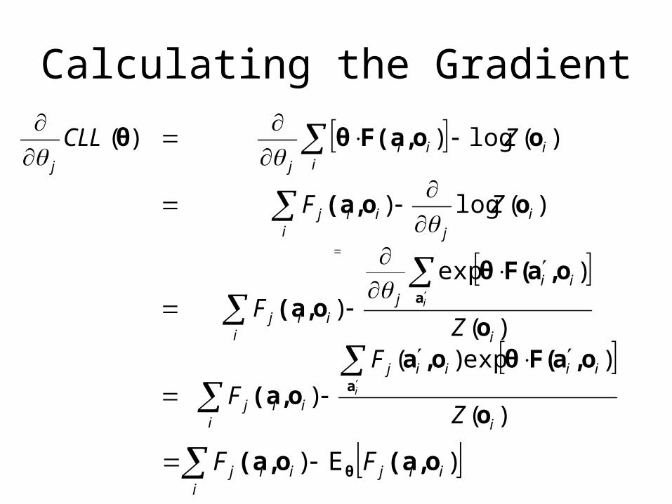
Calculating the Gradient
i i
iiiij
iij
i i
iij
iij
ii
jiij
iiii
jj
Z
F
F
ZF
ZF
ZCLL
i
i
)(
)exp)(
)
)(
)exp
)
)(log)
)(log))(
o
o,aF(θo,a
o,(a
o
o,aF(θ
o,(a
oo,(a
oo,F(aθθ
a
a
i
iijiij FF )E) o,(ao,(a θ


![CIS 895 – MSE PROJECTpeople.cs.ksu.edu/~sowji/100jiMSE/Phase3/Presentation3_20090413.pdfTERMS[3] Shallow Parsing/Chunking NLP technique that attempts to look for key phrases but](https://img.pdfslide.us/doc/110x75/5f5860b8da3e367ffa6582dd/cis-895-a-mse-sowji100jimsephase3presentation320090413pdf-terms3-shallow.jpg)