Embed Size (px)
Citation preview

Activity Detection in Videos
Riu BaringCIS 8590 Perception of Intelligent System
Temple University
Fall 2007

Outline
BackgroundRelated WorkThe ModelNormal CountEvent Count

Activity Detection Problems
A process like e.g., traffic flow, crowd formation, or financial electronic transactions is unfolding in time. We can monitor and observe the flow frequencies at many fixed time points. Typically, there are many causes influencing changes in these frequencies.

Causes for Change
Possible causes for change include: a) changes due to noise; i.e., those best
modeled by e.g., a Gaussian error distribution.
b) periodic changes; i.e., those expected to happen over periodic intervals.
c) changes not due to either of the above: these are usually the changes we would like to detect.
An Example: Building Data
•3 months of “people count”•30 minutes•Calit2 UC Irvine Campus

Another Example: Traffic Data•6 months of estimated vehicle count•Every 5 minutes •Glendale on-ramp to 101N, Los Angeles

More Examples
Detecting ‘Events’, which are not pre-planned, involving large numbers of people at a particular location.
Detecting ‘Fraudulent transactions’. We observe a variety of electronic transactions at many time intervals. We would like to detect when the number of transactions is significantly different from what is expected.

Related Work
Keogh et al. – KDD ‘02 Quantize real-valued time-series into finite set of symbols Then use a Markov model to detect surprising patterns in the
symbol sequence Guralnik and Srivastava – KDD ‘99
Iterative likelihood-based method for segmenting a time-series into homogeneous regions
Salmenkivi and Mannila (2005) Segmenting sets of low-level time-stamped events into time-
periods of relatively constant intensity using a combination of Poisson models and Bayesian estimation methods
Kleinberg – KDD ‘02 method based on an infinite automaton could be used to detect
bursty events in text streams

Related Work
All approaches share a common goal detection of novel and unusual data points or
segments in time-series.
None focuses on detection of bursty events embedded in time series of counts that reflect the normal diurnal and calendar patterns of human activity.
GOAL:
To automatically detect
the presence of unusual events
in the observation sequence.

Background
Markov-modulated Processes (Scott, 1998) Analysis of Web Surfing Behavior (Scott and Smyth, 2005) Telephone Network Fraud Detection (Scott, 2000)
Ihler et al (KDD 2006) developed a framework for building a probabilistic model of time-varying counting process in which a superposition of both time-varying but regular (periodic) and aperiodic processes were observed.

Method I
A Baseline Model
Where
ThresholdAdequate for:
Events interspersed in the data are sufficiently few
Events are sufficiently noticeable.

Chicken and Egg
Method I
Baseline Model
Ideal Model

Method I
False Positive, Persistence, and Duration
Baseline Model Baseline Model – Lower Threshold

Method II – Ideal Model
Observed Count
Normal Count (Unobserved)
Event Count (Unobserved )

Normal CountModeling Periodic
Count Data
d(t) = {1, …, 7}Sunday = 1, …
h(t) = intervali.e. half-hour

Periodic Components
Poisson Process Rate
Day Effect
Time of Day Effect

Event Count: The Process NE
Events signify times during which there are higher frequencies which are not due to periodic or noise causes. We can model this by introducing a binary latent process z(t) and assuming z(t)=1 for such events and z(t)=0 if not.
P(z(t)=1|z(t-1)=0)= 1-z00; P(z(t)=0|z(t-1)=0)= z00;
P(z(t)=1|z(t-1)=1)= z11; P(z(t)=0|z(t-1)=1)= 1-z11
i.e., if there is no event at time t-1, the chance of an event at time t is 1-z00
Modeling Rare Persistent
Events

Graphical Model

Priors for event probabilities
Beta distributions: priors for the z’s.
and z11 analogously.
This characterizes the behavior of the underlying latent process. The hyperparameters a,b are designed to model that behavior.
00 1100 0000 1 baz z z

Priors for event probabilities
Recall that N0(t) (the non-event process) characterizes periodic and noise changes. The event process NE(t) characterizes other changes.
NE(t) is 0 if z(t)=0 and Poisson with rate γ(t) if z(t)=1. So, if there is no event, N(t)=N0(t). If there is an event, the
frequency due to periodic or noise changes is N(t)=N0(t)+NE(t)
The rate γ(t) is itself gamma with parameters aE and bE. Hence (by conjugacy) it is marginally negative binomial (NB) with p=(bE/(1+bE) and n=N(t).

Gibbs Sampling
Gibbs sampling works by simulating each parameter/latent variable conditional on all the rest.
The λ’s are parameters and the z’s,N’s are the latent variables.
The resulting simulated values have an empirical distribution similar to the true posterior distribution. It works as a result of the fact that the joint distribution of parameters is determined by the set of all such conditional distributions.

Gibbs Sampling
Given z(t)=0 and the remaining parameters, Put N0(t)=N(t) and NE(t)=0.
If z(t)=1, simulate NE(t) as negative binomial with parameters, N(t) and bE/(1+bE). Put N0(t)=N(t)-NE(t).
To simulate z(t), define 0 0
0 0
-1 -100 0000
-1 -100 0000
0
1 (1- ) ( , ( ));
2 (1- ) (1- ) ( - , ( )) ;1
a b
Na b E
Ei
term z z z P N t
bterm z z z P N i t NB N i
b
=
=

More of Gibbs Sampling
Then, if the previous state was 0, we get:
0 0
0 00 0
-1 100 0000
00
-1 -1-1 -100 00 00 0000 00
0
(1- ) (1- ) ( - ; ( )) ; ;1
( ( ) 1) ;
(1- ) ( , ( )) (1- ) (1- ) ( - , ( )) ; ;1
Na b E
EiNa ab b E
Ei
bz z z P N i t NB N i
bP z t
bz z z P N t z z z P N i t NB N i
b
1 1
1 11 1
-1 -111 1111
01
-1 -1-1 -111 11 11 1111 11
0
( ) (1- ) ( - , ( )) ; ;1
( ( ) 1) ;
(1- ) (1- ) ( , ( )) ( ) (1- ) ( - , ( )) ; ;1
Na b E
EiNa ab b E
Ei
bz z z P N i t NB N i
bP z t
bz z z P N t z z z P N i t NB N i
b

Gibbs Sampling (Continued)
Having simulated z(t), we can simulate the parameters as follows:
Where ‘Nday’ denotes the number of ‘day’ units in the data, ‘Nhh’ denotes the number of ‘hh’ periods in the data.
; day day hh hhday hh
N N
bt
λ Γ N(t) + α,

Result: Building Data

Result: Freeway Traffic Data
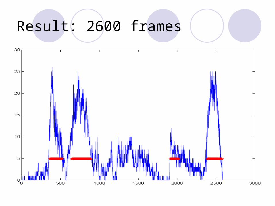
Result: 2600 frames


Discussion
Poisson process (nonhomogeneous).
Able to detect activity at the expected frame.

Future Work
Histogram of direction implementation

References
1. A. Ihler, J. Hutchins, and P. Smyth, “Adaptive event detection with time-varying Poissons process,” KDD 2006.
2. S. L. Scott and P. Smyth, “The Markov modulated Poisson process and Markov Poisson cascade with applications to web traffic data,” Bayesian Statistics, vol. 7, pp. 671-680, 2003.
3. S. L. Scott, “Detecting network intrusion using a Markov modulated nonhomogeneous Poisson process,” http://www-rcf.usc.edu/~sls/mmnhpp.ps.gz, 2004.
4. S. L. Scott, “Bayesian methods and extensions for the two state Markov modulated Poisson process,” Ph.D. dissertation, Harvard University, Dept. of Statistics, 1998.