Basic Principles of RF Superconductivity and ... · PDF fileBasic Principles of RF Superconductivity and Superconducting Cavities 1 ... The vanishing electrical resistance of ... machine

Basic Principles of RF Superconductivity and Superconducting Cavities 1

Peter SchmuserInstitut fur Experimentalphysik

Universitat Hamburg

Abstract

The basics of superconductivity are outlined with special emphasis on the features which are relevantfor the application of superconductors in radio frequency cavities for particle acceleration. For a cylindricalresonator (“pill box cavity”) the electromagnetic field in the cavity and important parameters such asresonance frequency, quality factor and shunt impedance are calculated analytically. The design andperformance of practical cavities is shortly addressed.

1 Introduction

1.1 Advantages and limitations of superconductor technology in accelerators

The vanishing electrical resistance of superconducting coils as well as their ability to provide magnetic fieldsfar beyond those of saturated iron is the main motivation for using superconducting (sc) magnets in allnew large proton, antiproton and heavy ion accelerators2. Superconductivity does not only open the way tomuch higher particle energies but at the same time leads to a substantial reduction of operating costs. Inthe normal-conducting Super Proton Synchrotron SPS at CERN a power of 52 MW is needed to operate themachine at an energy of 315 GeV while at HERA a cryogenic plant with 6 MW electrical power consumptionis sufficient to provide the cooling of the superconducting magnets with a stored proton beam of 920 GeV.Hadron energies in the TeV regime are practically inaccessible with standard magnet technology. Anotherimportant application of superconducting materials is in the large experiments at hadron or lepton colliderswhere superconducting detector magnets are far superior to normal magnets.

In the case of accelerating cavities the advantage of superconductors is not at all that obvious. In fact,three of the proposed linear electron positron colliders are based on copper acceleration structures: the‘Next Linear Collider’ NLC [3] at Stanford, the ‘Japanese Linear Collider’ JLC [4] at Tsukuba, and the‘Compact Linear Collider’ CLIC [5] at CERN, while only the international TESLA project [6, 7] uses scniobium cavities. The traditional arguments against superconductor technology in linear colliders have beenthe low accelerating fields achieved in sc cavities and the high cost of cryogenic equipment. Superconductingcavities face a strong physical limitation: the microwave magnetic field must stay below the critical fieldof the superconductor. For the best superconductor for cavities, niobium, this corresponds to a maximumaccelerating field of about 45 MV/m while normal-conducting cavities operating at high frequency (above5 GHz) should in principle be able to reach 100 MV/m or more. In practice, however, sc cavities were oftenfound to be limited at much lower fields of some 5 MV/m and hence were totally non-competitive for alinear collider. Great progress was achieved with the 340 five-cell cavities of the Continuous Electron BeamAccelerator Facility CEBAF [8] at Jefferson Laboratory in Virginia, USA. These 1.5 GHz niobium cavitieswere developed at Cornell University and produced by industry. They exceeded the design gradient of 5MV/m and achieved 8.4 MV/m after installation in the accelerator (in several specially prepared cavitieseven 15-20 MV/m were reached). Building upon the CEBAF experience the intensive R&D of the TESLAcollaboration has succeeded in raising the accelerating field in multicell cavities to more than 25 MV/m.There is a realistic chance to reach even 35 MV/m, and to reduce substantially the cost for the cryogenicinstallation.

While superconducting magnets operated with direct current are free of energy dissipation, this is not thecase in microwave cavities. The non-superconducting electrons (see sect. 2) experience forced oscillations inthe time-varying magnetic field and dissipate power in the material. Although the resulting heat depositionis many orders of magnitude smaller than in copper cavities it constitutes a significant heat load on the

1Adapted from a review article in Prog. Part. Nucl. Phys. [1].2The parameters of high energy lepton and hadron colliders are summarized in [2].

Proceedings of the 11th Workshop on RF Superconductivity, Lübeck/Travemünder, Germany

180 MOT01

refrigeration system. As a rule of thumb, 1 W of heat deposited at 2 K requires almost 1 kW of primaryac power in the refrigerator. Nevertheless, there is now a worldwide consensus that the overall efficiencyfor converting primary electric power into beam power is about a factor two higher for a superconductingthan for a normal-conducting linear collider with optimized parameters in either case [9]. Another definiteadvantage of a superconducting collider is the low resonance frequency of the cavities that can be chosen(1.3 GHz in TESLA). The longitudinal (transverse) wake fields generated by the ultrashort electron bunchesupon passing the cavities scale with the second (third) power of the frequency and are hence much smallerin TESLA than in NLC (f = 11 GHz). The wake fields may have a negative impact on the beam emittance(the area occupied in phase space) and on the luminosity of the collider.

1.2 Characteristic properties of superconducting cavities

The fundamental advantage of superconducting niobium cavities is the extremely low surface resistance of afew nano-ohms at 2 Kelvin as compared to several milli-ohms in copper cavities. The quality factor Q0 (2πtimes the ratio of stored energy to energy loss per cycle) is inversely proportional to the surface resistanceand may exceed 1010. Only a tiny fraction of the incident radio frequency (rf) power is dissipated in thecavity walls, the lion’s share is transferred to the beam. The physical limitation of a sc resonator is givenby the requirement that the rf magnetic field at the inner surface has to stay below the critical field of thesuperconductor (about 190 mT for niobium), corresponding to an accelerating field of Eacc = 45 MV/m.In principle the quality factor should stay constant when approaching this fundamental superconductorlimit but in practice the curve Q0 = Q0(Eacc) ends at considerably lower values, often accompanied witha strong decrease of Q0 towards the highest gradient reached in the cavity. The main reasons for theperformance degradation are excessive heating caused by impurities on the inner surface or by field emissionof electrons. The cavity becomes partially normal-conducting, associated with strongly enhanced powerdissipation. Because of the exponential increase of surface resistance with temperature this may result in arun-away effect and eventually a quench of the entire cavity.Field emission of electrons from sharp tips is the most severe limitation in high-gradient superconductingcavities. Small particles on the cavity surface act as field emitters. By applying the clean room techniquesdeveloped in semiconductor industry it has been possible to raise the threshold for field emission in multicellcavities from about 10 MV/m to more than 20 MV/m in the past few years. The preparation of a smoothand almost mirror-like surface by electrolytic polishing is another important improvement.A detailed description of sc cavities is found in [10].

2 Basics of Superconductivity

The unusual features of superconducting magnets and cavities are closely linked to the physical propertiesof the superconductor itself. For this reason a basic understanding of superconductivity is indispensablefor the design, construction and operation of superconducting accelerator components. Only the traditional‘low-temperature’ superconductors are treated since up to date the use of ‘high-temperature’ ceramic su-perconductors in these devices is rather limited [11, 12]. For more comprehensive presentations I refer tothe excellent text books by W. Buckel [13] and by D.R. Tilley and J. Tilley [14].

2.1 Overview

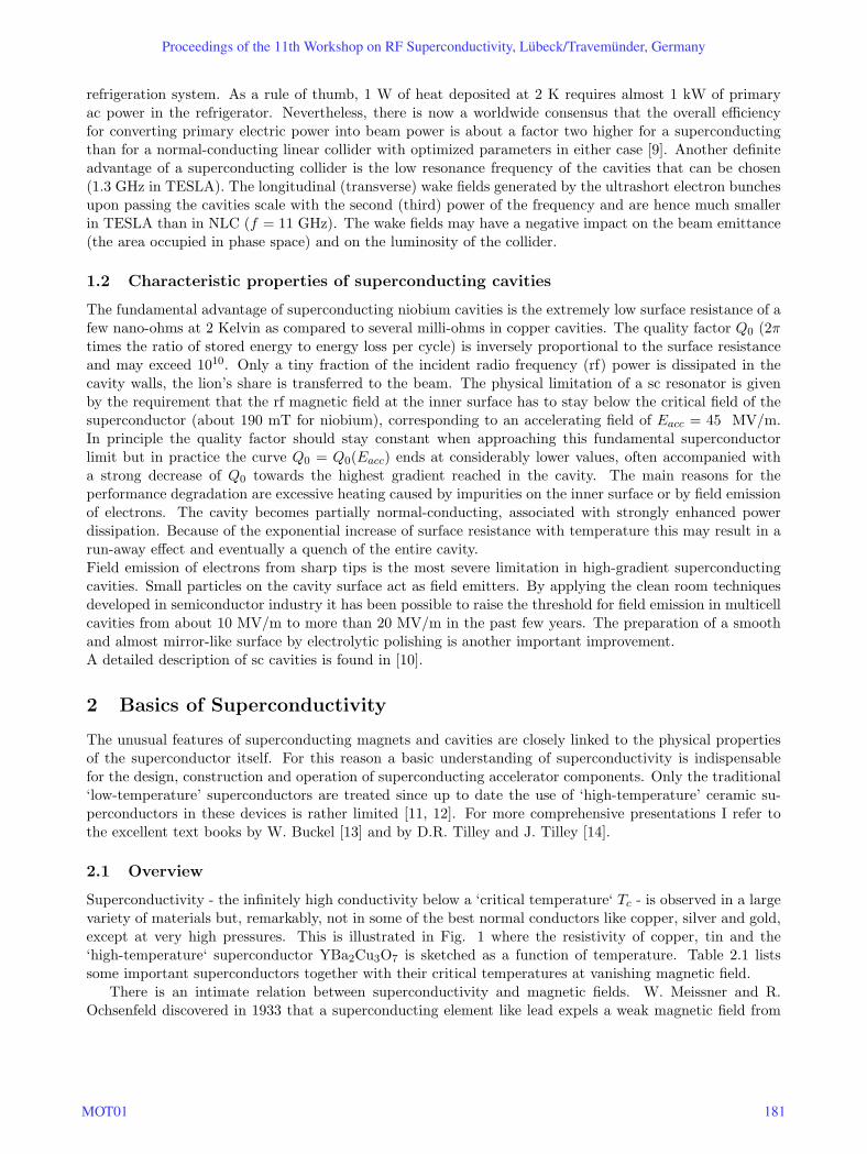
Superconductivity - the infinitely high conductivity below a ‘critical temperature‘ Tc - is observed in a largevariety of materials but, remarkably, not in some of the best normal conductors like copper, silver and gold,except at very high pressures. This is illustrated in Fig. 1 where the resistivity of copper, tin and the‘high-temperature‘ superconductor YBa2Cu3O7 is sketched as a function of temperature. Table 2.1 listssome important superconductors together with their critical temperatures at vanishing magnetic field.

There is an intimate relation between superconductivity and magnetic fields. W. Meissner and R.Ochsenfeld discovered in 1933 that a superconducting element like lead expels a weak magnetic field from


MOT01 181

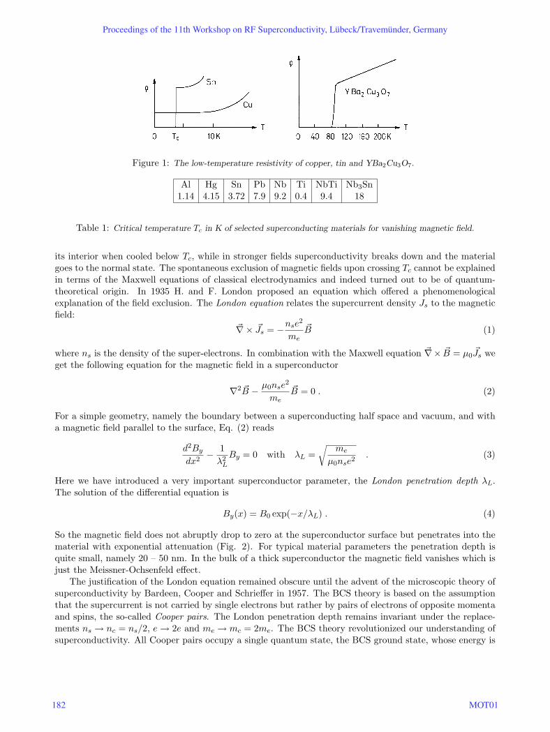
Figure 1: The low-temperature resistivity of copper, tin and YBa2Cu3O7.

Al Hg Sn Pb Nb Ti NbTi Nb3Sn1.14 4.15 3.72 7.9 9.2 0.4 9.4 18

Table 1: Critical temperature Tc in K of selected superconducting materials for vanishing magnetic field.

its interior when cooled below Tc, while in stronger fields superconductivity breaks down and the materialgoes to the normal state. The spontaneous exclusion of magnetic fields upon crossing Tc cannot be explainedin terms of the Maxwell equations of classical electrodynamics and indeed turned out to be of quantum-theoretical origin. In 1935 H. and F. London proposed an equation which offered a phenomenologicalexplanation of the field exclusion. The London equation relates the supercurrent density Js to the magneticfield:

~∇× ~Js = −nse2

me

~B (1)

where ns is the density of the super-electrons. In combination with the Maxwell equation ~∇× ~B = µ0~Js we

get the following equation for the magnetic field in a superconductor

∇2 ~B − µ0nse2

me

~B = 0 . (2)

For a simple geometry, namely the boundary between a superconducting half space and vacuum, and witha magnetic field parallel to the surface, Eq. (2) reads

d2By

dx2− 1

λ2L

By = 0 with λL =√

me

µ0nse2. (3)

Here we have introduced a very important superconductor parameter, the London penetration depth λL.The solution of the differential equation is

By(x) = B0 exp(−x/λL) . (4)

So the magnetic field does not abruptly drop to zero at the superconductor surface but penetrates into thematerial with exponential attenuation (Fig. 2). For typical material parameters the penetration depth isquite small, namely 20 – 50 nm. In the bulk of a thick superconductor the magnetic field vanishes which isjust the Meissner-Ochsenfeld effect.

The justification of the London equation remained obscure until the advent of the microscopic theory ofsuperconductivity by Bardeen, Cooper and Schrieffer in 1957. The BCS theory is based on the assumptionthat the supercurrent is not carried by single electrons but rather by pairs of electrons of opposite momentaand spins, the so-called Cooper pairs. The London penetration depth remains invariant under the replace-ments ns → nc = ns/2, e→ 2e and me → mc = 2me. The BCS theory revolutionized our understanding ofsuperconductivity. All Cooper pairs occupy a single quantum state, the BCS ground state, whose energy is


182 MOT01

Figure 2: The exponential drop of the magnetic field and the rise of the Cooper-pair density at a boundary between

a normal and a superconductor.

separated from the single-electron states by a temperature dependent energy gap Eg = 2∆(T ). The criticaltemperature is related to the energy gap at T = 0 by

1.76 kBTc = ∆(0) . (5)

Here kB = 1.38 · 10−23 J/K is the Boltzmann constant. The magnetic flux through a superconducting ringis found to be quantized, the smallest unit being the elementary flux quantum

Φ0 =h

2e= 2.07 · 10−15 Vs . (6)

These and many other predictions of the BCS theory, like the temperature dependence of the energy gapand the existence of quantum interference phenomena, have been confirmed by experiment and often foundpractical application.

A discovery of enormous practical consequences was the finding that there exist two types of supercon-ductors with rather different response to magnetic fields. The elements lead, mercury, tin, aluminium andothers are called ’type I‘ superconductors. They do not admit a magnetic field in the bulk material andare in the superconducting state provided the applied field stays below a critical field Hc (Bc = µ0Hc isusually less than 0.1 Tesla). All superconducting alloys like lead-indium, niobium-titanium, niobium-tin andalso the element niobium belong to the large class of ’type II‘ superconductors. They are characterized bytwo critical fields, Hc1 and Hc2. Below Hc1 these substances are in the Meissner phase with complete fieldexpulsion while in the range Hc1 < H < Hc2 they enter the mixed phase in which the magnetic field piercesthe bulk material in the form of flux tubes. Many of these materials remain superconductive up to muchhigher fields (10 Tesla or more).

2.2 Energy balance in a magnetic field

A material like lead makes a phase transition from the normal to the superconducting state when it iscooled below Tc and when the magnetic field is less than Hc(T ). This is a phase transition comparable tothe transition from water to ice below 0C. Phase transitions take place when the new state is energeticallyfavoured. The relevant thermodynamic energy is here the so-called Gibbs free energy G. Free energieshave been measured for a variety of materials. For temperatures T < Tc they are found to be lower inthe superconducting than in the normal state while Gsup approaches Gnorm in the limit T → Tc, see Fig.3a. What is now the impact of a magnetic field on the energy balance? A magnetic field has an energydensity µ0/2 · H2, and according to the Meissner-Ochsenfeld effect the magnetic energy must be pushedout of the material when it enters the superconducting state. Hence the free energy per unit volume in thesuperconducting state increases quadratically with the applied field:

Gsup(H) = Gsup(0) +µ0

2H2 . (7)


MOT01 183

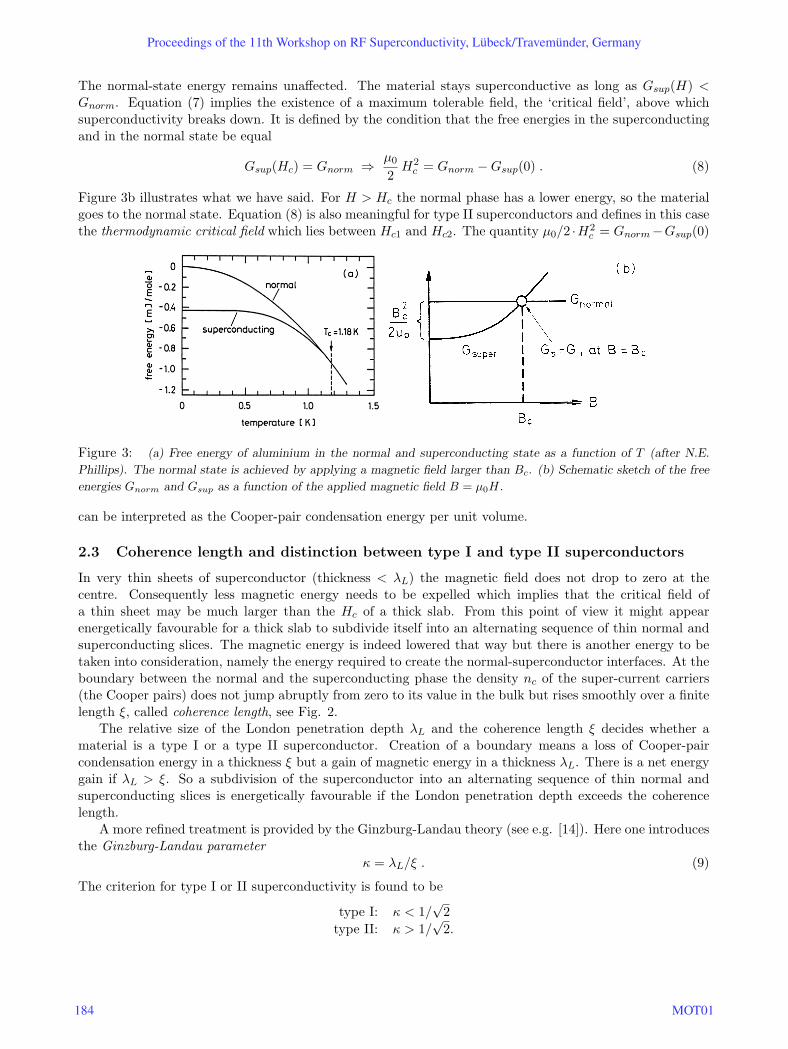
The normal-state energy remains unaffected. The material stays superconductive as long as Gsup(H) <Gnorm. Equation (7) implies the existence of a maximum tolerable field, the ‘critical field’, above whichsuperconductivity breaks down. It is defined by the condition that the free energies in the superconductingand in the normal state be equal

Gsup(Hc) = Gnorm ⇒ µ0

2H2

c = Gnorm −Gsup(0) . (8)

Figure 3b illustrates what we have said. For H > Hc the normal phase has a lower energy, so the materialgoes to the normal state. Equation (8) is also meaningful for type II superconductors and defines in this casethe thermodynamic critical field which lies between Hc1 and Hc2. The quantity µ0/2 ·H2

c = Gnorm−Gsup(0)

Figure 3: (a) Free energy of aluminium in the normal and superconducting state as a function of T (after N.E.

Phillips). The normal state is achieved by applying a magnetic field larger than Bc. (b) Schematic sketch of the free

energies Gnorm and Gsup as a function of the applied magnetic field B = µ0H.

can be interpreted as the Cooper-pair condensation energy per unit volume.

2.3 Coherence length and distinction between type I and type II superconductors

In very thin sheets of superconductor (thickness < λL) the magnetic field does not drop to zero at thecentre. Consequently less magnetic energy needs to be expelled which implies that the critical field ofa thin sheet may be much larger than the Hc of a thick slab. From this point of view it might appearenergetically favourable for a thick slab to subdivide itself into an alternating sequence of thin normal andsuperconducting slices. The magnetic energy is indeed lowered that way but there is another energy to betaken into consideration, namely the energy required to create the normal-superconductor interfaces. At theboundary between the normal and the superconducting phase the density nc of the super-current carriers(the Cooper pairs) does not jump abruptly from zero to its value in the bulk but rises smoothly over a finitelength ξ, called coherence length, see Fig. 2.

The relative size of the London penetration depth λL and the coherence length ξ decides whether amaterial is a type I or a type II superconductor. Creation of a boundary means a loss of Cooper-paircondensation energy in a thickness ξ but a gain of magnetic energy in a thickness λL. There is a net energygain if λL > ξ. So a subdivision of the superconductor into an alternating sequence of thin normal andsuperconducting slices is energetically favourable if the London penetration depth exceeds the coherencelength.

A more refined treatment is provided by the Ginzburg-Landau theory (see e.g. [14]). Here one introducesthe Ginzburg-Landau parameter

κ = λL/ξ . (9)

The criterion for type I or II superconductivity is found to be

type I: κ < 1/√

2type II: κ > 1/

√2.


184 MOT01

The following table lists the penetration depths and coherence lengths of some important superconductingelements. Niobium is a type II conductor but close to the border to type I, while indium, lead and tin areclearly in the type I class.

material In Pb Sn NbλL [nm] 24 32 ≈ 30 32ξ [nm] 360 510 ≈ 170 39

The coherence length ξ is proportional to the mean free path of the conduction electrons in the metal. Inalloys the mean free path is generally much shorter than in pure metals hence alloys are always type IIconductors.

In reality a type II superconductor is not subdivided into thin slices but the field penetrates the samplein the form of flux tubes which arrange themselves in a triangular pattern which can be made visible byevaporating iron atoms onto a superconductor surface sticking out of the liquid helium. The fluxoid patternshown in Fig. 4a proves beyond any doubt that niobium is indeed a type II superconductor. Each flux tubeor fluxoid contains one elementary flux quantum Φ0 which is surrounded by a Cooper-pair vortex current.The centre of a fluxoid is normal-conducting and covers an area of roughly πξ2. When we apply an externalfield H, fluxoids keep moving into the specimen until their average magnetic flux density is identical toB = µ0H. The fluxoid spacing in the triangular lattice d =

√2Φ0/(

√3B) amounts to 20 nm at 6 Tesla.

The upper critical field is reached when the current vortices of the fluxoids start touching each other atwhich point superconductivity breaks down. In the Ginzburg-Landau theory the upper critical field is givenby

Bc2 =√

2 κ Bc =Φ0

2πξ2. (10)

For niobium-titanium with an upper critical field Bc2 = 14 T this formula yields ξ = 5nm. The coherencelength is larger than the typical width of a grain boundary in NbTi which means that the supercurrent canfreely move from grain to grain. In high-Tc superconductors the coherence length is often shorter than thegrain boundary width, and then current flow from one grain to the next is strongly impeded.

2.4 Flux flow resistance and flux pinning

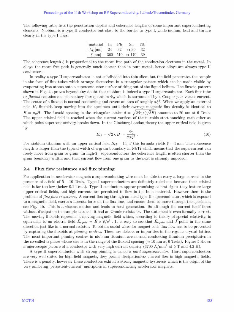
For application in accelerator magnets a superconducting wire must be able to carry a large current in thepresence of a field of 5 – 10 Tesla. Type I superconductors are definitely ruled out because their criticalfield is far too low (below 0.1 Tesla). Type II conductors appear promising at first sight: they feature largeupper critical fields, and high currents are permitted to flow in the bulk material. However there is theproblem of flux flow resistance. A current flowing through an ideal type II superconductor, which is exposedto a magnetic field, exerts a Lorentz force on the flux lines and causes them to move through the specimen,see Fig. 4b. This is a viscous motion and leads to heat generation. So although the current itself flowswithout dissipation the sample acts as if it had an Ohmic resistance. The statement is even formally correct.The moving fluxoids represent a moving magnetic field which, according to theory of special relativity, isequivalent to an electric field ~Eequiv = ~B × ~v/c2 . It is easy to see that ~Eequiv and ~J point in the samedirection just like in a normal resistor. To obtain useful wires for magnet coils flux flow has to be preventedby capturing the fluxoids at pinning centres. These are defects or impurities in the regular crystal lattice.The most important pinning centres in niobium-titanium are normal-conducting titanium precipitates inthe so-called α phase whose size is in the range of the fluxoid spacing (≈ 10 nm at 6 Tesla). Figure 5 showsa microscopic picture of a conductor with very high current density (3700 A/mm2 at 5 T and 4.2 K).

A type II superconductor with strong pinning is called a hard superconductor. Hard superconductorsare very well suited for high-field magnets, they permit dissipationless current flow in high magnetic fields.There is a penalty, however: these conductors exhibit a strong magnetic hysteresis which is the origin of thevery annoying ’persistent-current‘ multipoles in superconducting accelerator magnets.


MOT01 185

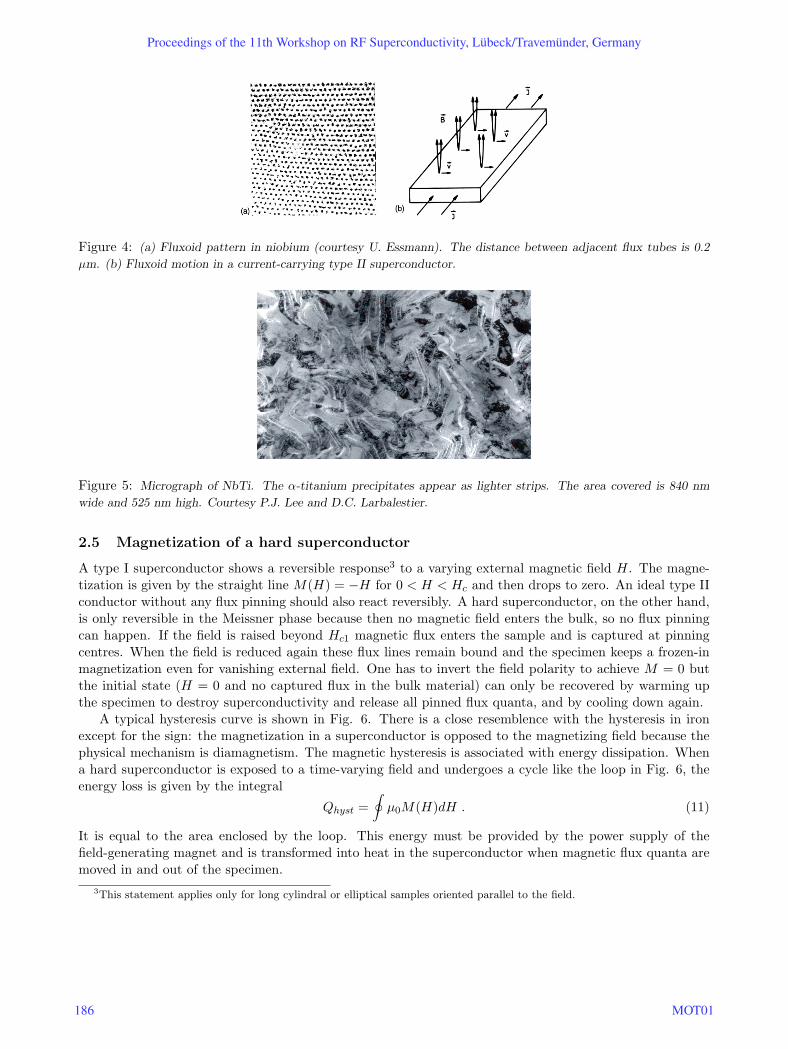
Figure 4: (a) Fluxoid pattern in niobium (courtesy U. Essmann). The distance between adjacent flux tubes is 0.2

µm. (b) Fluxoid motion in a current-carrying type II superconductor.

Figure 5: Micrograph of NbTi. The α-titanium precipitates appear as lighter strips. The area covered is 840 nm

wide and 525 nm high. Courtesy P.J. Lee and D.C. Larbalestier.

2.5 Magnetization of a hard superconductor

A type I superconductor shows a reversible response3 to a varying external magnetic field H. The magne-tization is given by the straight line M(H) = −H for 0 < H < Hc and then drops to zero. An ideal type IIconductor without any flux pinning should also react reversibly. A hard superconductor, on the other hand,is only reversible in the Meissner phase because then no magnetic field enters the bulk, so no flux pinningcan happen. If the field is raised beyond Hc1 magnetic flux enters the sample and is captured at pinningcentres. When the field is reduced again these flux lines remain bound and the specimen keeps a frozen-inmagnetization even for vanishing external field. One has to invert the field polarity to achieve M = 0 butthe initial state (H = 0 and no captured flux in the bulk material) can only be recovered by warming upthe specimen to destroy superconductivity and release all pinned flux quanta, and by cooling down again.

A typical hysteresis curve is shown in Fig. 6. There is a close resemblence with the hysteresis in ironexcept for the sign: the magnetization in a superconductor is opposed to the magnetizing field because thephysical mechanism is diamagnetism. The magnetic hysteresis is associated with energy dissipation. Whena hard superconductor is exposed to a time-varying field and undergoes a cycle like the loop in Fig. 6, theenergy loss is given by the integral

Qhyst =∮

µ0M(H)dH . (11)

It is equal to the area enclosed by the loop. This energy must be provided by the power supply of thefield-generating magnet and is transformed into heat in the superconductor when magnetic flux quanta aremoved in and out of the specimen.

3This statement applies only for long cylindral or elliptical samples oriented parallel to the field.


186 MOT01

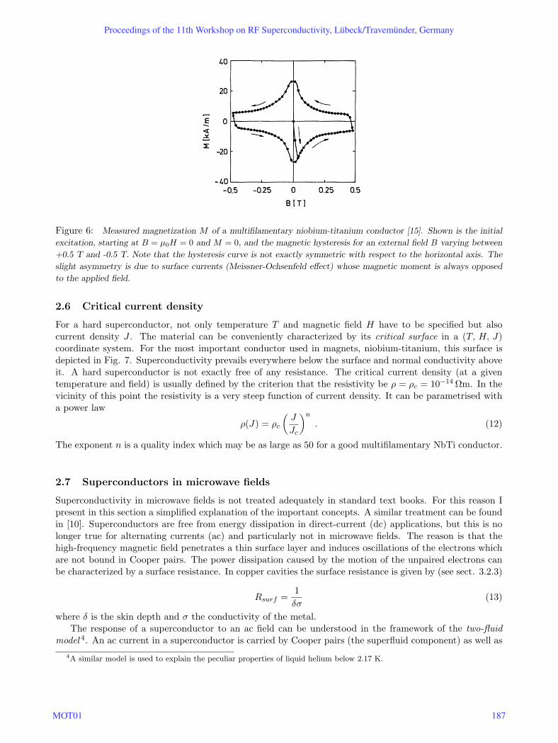
Figure 6: Measured magnetization M of a multifilamentary niobium-titanium conductor [15]. Shown is the initial

excitation, starting at B = µ0H = 0 and M = 0, and the magnetic hysteresis for an external field B varying between

+0.5 T and -0.5 T. Note that the hysteresis curve is not exactly symmetric with respect to the horizontal axis. The

slight asymmetry is due to surface currents (Meissner-Ochsenfeld effect) whose magnetic moment is always opposed

to the applied field.

2.6 Critical current density

For a hard superconductor, not only temperature T and magnetic field H have to be specified but alsocurrent density J . The material can be conveniently characterized by its critical surface in a (T, H, J)coordinate system. For the most important conductor used in magnets, niobium-titanium, this surface isdepicted in Fig. 7. Superconductivity prevails everywhere below the surface and normal conductivity aboveit. A hard superconductor is not exactly free of any resistance. The critical current density (at a giventemperature and field) is usually defined by the criterion that the resistivity be ρ = ρc = 10−14 Ωm. In thevicinity of this point the resistivity is a very steep function of current density. It can be parametrised witha power law

ρ(J) = ρc

(J

Jc

)n

. (12)

The exponent n is a quality index which may be as large as 50 for a good multifilamentary NbTi conductor.

2.7 Superconductors in microwave fields

Superconductivity in microwave fields is not treated adequately in standard text books. For this reason Ipresent in this section a simplified explanation of the important concepts. A similar treatment can be foundin [10]. Superconductors are free from energy dissipation in direct-current (dc) applications, but this is nolonger true for alternating currents (ac) and particularly not in microwave fields. The reason is that thehigh-frequency magnetic field penetrates a thin surface layer and induces oscillations of the electrons whichare not bound in Cooper pairs. The power dissipation caused by the motion of the unpaired electrons canbe characterized by a surface resistance. In copper cavities the surface resistance is given by (see sect. 3.2.3)

Rsurf =1δσ

(13)

where δ is the skin depth and σ the conductivity of the metal.The response of a superconductor to an ac field can be understood in the framework of the two-fluid

model 4. An ac current in a superconductor is carried by Cooper pairs (the superfluid component) as well as4A similar model is used to explain the peculiar properties of liquid helium below 2.17 K.


MOT01 187

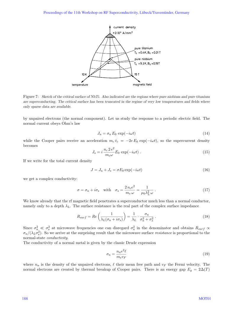
Figure 7: Sketch of the critical surface of NbTi. Also indicated are the regions where pure niobium and pure titanium

are superconducting. The critical surface has been truncated in the regime of very low temperatures and fields where

only sparse data are available.

by unpaired electrons (the normal component). Let us study the response to a periodic electric field. Thenormal current obeys Ohm’s law

Jn = σn E0 exp(−iωt) (14)

while the Cooper pairs receive an acceleration mc vc = −2eE0 exp(−iωt), so the supercurrent densitybecomes

Js = inc 2 e2

meωE0 exp(−iωt) . (15)

If we write for the total current density

J = Jn + Js = σE0 exp(−iωt) (16)

we get a complex conductivity:

σ = σn + iσs with σs =2 nce

2

me ω=

1µ0λ2

L ω. (17)

We know already that the rf magnetic field penetrates a superconductor much less than a normal conductor,namely only to a depth λL. The surface resistance is the real part of the complex surface impedance

Rsurf = Re

(1

λL(σn + iσs)

)=

1λL· σn

σ2n + σ2

s

. (18)

Since σ2n σ2

s at microwave frequencies one can disregard σ2n in the denominator and obtains Rsurf ∝

σn/(λLσ2s). So we arrive at the surprising result that the microwave surface resistance is proportional to the

normal-state conductivity.The conductivity of a normal metal is given by the classic Drude expression

σn =nne2`

mevF(19)

where nn is the density of the unpaired electrons, ` their mean free path and vF the Fermi velocity. Thenormal electrons are created by thermal breakup of Cooper pairs. There is an energy gap Eg = 2∆(T )


188 MOT01

between the BCS ground state and the free electron states. By analogy with the conductivity of an intrinsic(undoped) semiconductor we get nn ∝ exp(−Eg/(2kBT )) and hence

σn ∝ ` exp(−∆(T )/(kBT )) . (20)

Using 1/σs = µ0λ2Lω and ∆(T ) ≈ ∆(0) = 1.76kBTc we finally obtain for the BCS surface resistance

RBCS ∝ λ3L ω2 ` exp(−1.76 Tc/T ) . (21)

This formula displays two important aspects of microwave superconductivity: the surface resistance dependsexponentially on temperature, and it is proportional to the square of the rf frequency.

3 Design Principles and Properties of Superconducting Cavities

3.1 Choice of superconductor

In principle the critical temperature of the superconductor should be as high as possible. However, coppercavities coated with a high-Tc superconductor layer have shown unsatisfactory performance [11], therefore thehelium-cooled low-Tc superconductors are applied. In contrast to magnets were hard superconductors withlarge upper critical field (10–20 T) are needed, the superconductor in microwave applications is not limitedby the upper critical field but rather by the thermodynamic critical field (or possibly the ‘superheating field’)which is well below 0.5 T for all known superconducting elements and alloys. Moreover, strong flux pinningappears undesirable as it is coupled with hysteretic losses. Hence a ‘soft’ superconductor must be used, andpure niobium is the best candidate although its critical temperature is only 9.2 K and the thermodynamiccritical field about 190 mT. Niobium-tin (Nb3Sn) may appear more favorable since it has a higher criticaltemperature of 18 K and a superheating field of 400 mT; however, the gradients achieved in Nb3Sn coatedcopper cavities were below 15 MV/m, probably due to grain boundary effects in the Nb3Sn layer [16]. Forthese reasons pure niobium has been chosen in all large scale installations of sc cavities. There remain twochoices for the cavity layout: the cavity is made from copper and the inner surface is coated with a thin layerof Nb or, alternatively, the cavity is made from solid Nb. The former approach has been taken with greatsuccess with the 350 MHz cavities of the Large Electron Positron ring LEP at CERN. In the TESLA linearcollider, however, gradients of more than 25 MV/m are needed, and these are presently only accessible withcavities made from solid niobium. A high thermal conductivity is needed to guide the heat generated at theinner cavity surface through the wall to the liquid helium coolant. For this reason, the material must be ofextreme purity with contaminations in the ppm range.

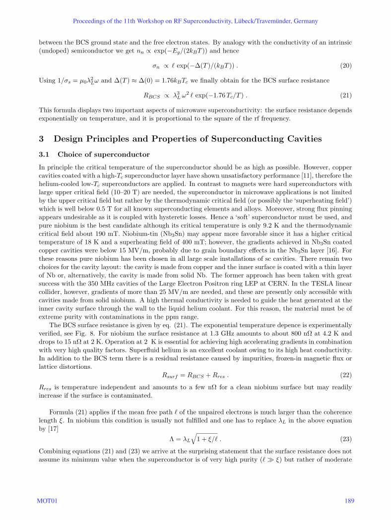
The BCS surface resistance is given by eq. (21). The exponential temperature depence is experimentallyverified, see Fig. 8. For niobium the surface resistance at 1.3 GHz amounts to about 800 nΩ at 4.2 K anddrops to 15 nΩ at 2 K. Operation at 2 K is essential for achieving high accelerating gradients in combinationwith very high quality factors. Superfluid helium is an excellent coolant owing to its high heat conductivity.In addition to the BCS term there is a residual resistance caused by impurities, frozen-in magnetic flux orlattice distortions.

Rsurf = RBCS + Rres . (22)

Rres is temperature independent and amounts to a few nΩ for a clean niobium surface but may readilyincrease if the surface is contaminated.

Formula (21) applies if the mean free path ` of the unpaired electrons is much larger than the coherencelength ξ. In niobium this condition is usually not fulfilled and one has to replace λL in the above equationby [17]

Λ = λL

√1 + ξ/` . (23)

Combining equations (21) and (23) we arrive at the surprising statement that the surface resistance does notassume its minimum value when the superconductor is of very high purity (` ξ) but rather of moderate


MOT01 189

2 3 4 5 6 7

RS [nΩ]

Tc/T

Rres

= 3 nΩ

1000

100

10

1

RBCS

1,00E-07

1,00E-06

1,00E-05

1,00E-04

1,00E+00 1,00E+01 1,00E+02 1,00E+03 1,00E+04 1,00E+05

Figure 8: Left: The surface resistance of a 9-cell TESLA cavity plotted as a function of Tc/T . The residual resistance

of 3 nΩ corresponds to a quality factor Q0 = 1011. Right: The microwave surface resistance of niobium as a function

of the mean free path ` of the unpaired electrons for a temperature of 4.25 K. Solid curve: two-fluid model; dashed

curves: model calculations by Halbritter [18] based on the BCS theory.

purity with a mean free path ` ≈ ξ, see Fig. 8. The measured BCS resistance in the sputter-coated LEPcavities is in fact a factor of two lower than in bulk niobium cavities [19]. The sputtered niobium layer hasa low RRR (see sect. 3.6) and an electron mean free path ` ≈ ξ.

3.2 Pill box cavity

The simplest model of an accelerating cavity is a hollow cylinder which is often called pill box. When thebeam pipes are neglected the field pattern inside the resonator and all relevant cavity parameters can becalculated analytically.

3.2.1 Field pattern

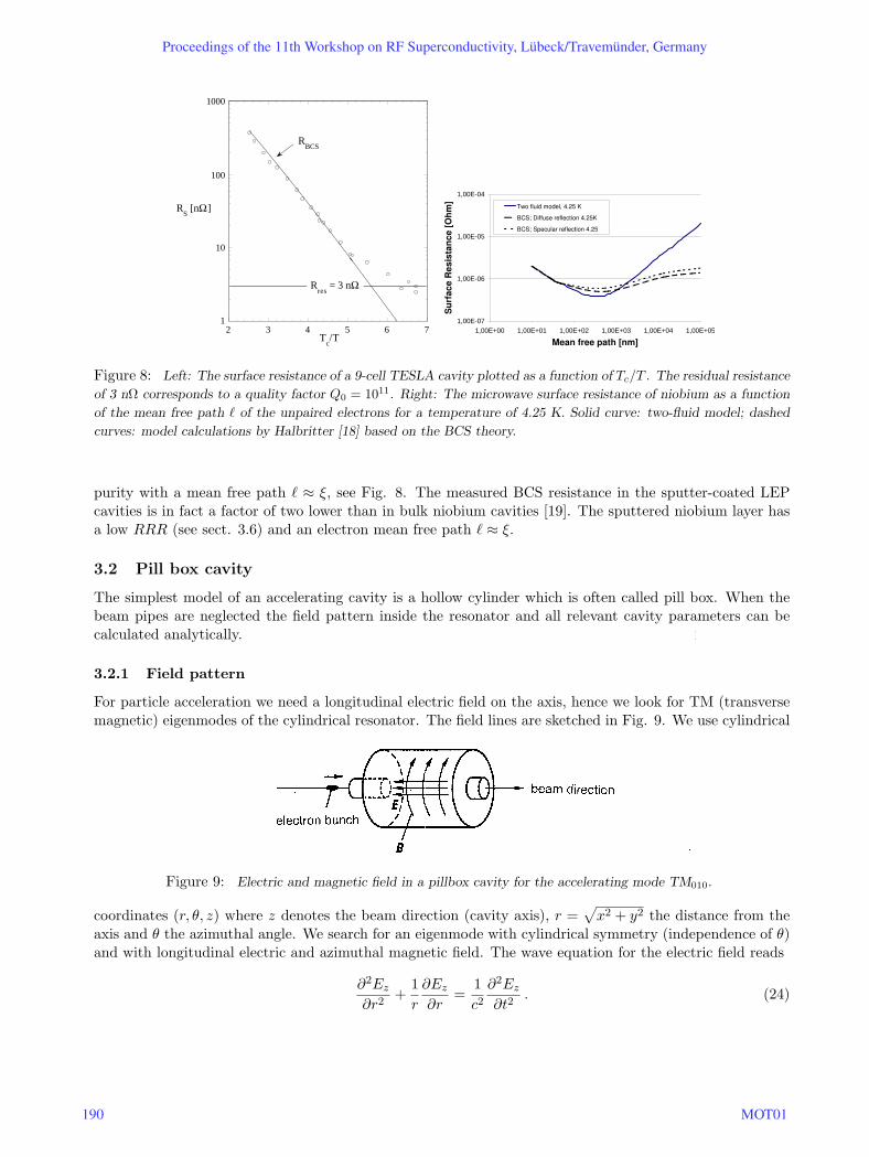
For particle acceleration we need a longitudinal electric field on the axis, hence we look for TM (transversemagnetic) eigenmodes of the cylindrical resonator. The field lines are sketched in Fig. 9. We use cylindrical

Figure 9: Electric and magnetic field in a pillbox cavity for the accelerating mode TM010.

coordinates (r, θ, z) where z denotes the beam direction (cavity axis), r =√

x2 + y2 the distance from theaxis and θ the azimuthal angle. We search for an eigenmode with cylindrical symmetry (independence of θ)and with longitudinal electric and azimuthal magnetic field. The wave equation for the electric field reads

∂2Ez

∂r2+

1r

∂Ez

∂r=

1c2

∂2Ez

∂t2. (24)


190 MOT01

For a harmonic time dependence Ez(r) cos(ωt) and with the new variable u = rω/c one obtains

∂2Ez

∂u2+

1u

∂Ez

∂u+ Ez(u) = 0 . (25)

This is the Bessel equation of zero order with the solution J0(u). Hence the radial dependence of the electricfield is

Ez(r) = E0J0(ωr

c) . (26)

For a perfectly conducting cylinder of radius Rc the longitudinal electric field must vanish at r = Rc, soJ0(ωRc/c) = 0. The first zero of J0(u) is at u = 2.405. This defines the frequency of the lowest eigenmode(we call it the fundamental mode in the following):

f0 =2.405c

2πRc, ω0 =

2.405c

Rc. (27)

In a cylindrical cavity the frequency does not depend on the length Lc. The magnetic field can be computedfrom the equation

∂Ez

∂r= µ0

∂Hθ

∂t. (28)

Hence we obtain for the fundamental TM mode

Ez(r, t) = E0J0(ω0r

c) cos(ω0t) ,

Hθ(r, t) = − E0

µ0cJ1(

ω0r

c) sin(ω0t) . (29)

Electric and magnetic field are 90 out of phase. The azimuthal magnetic field vanishes on the axis andassumes its maximum close to the cavity wall.

3.2.2 Stored energy

The electromagnetic field energy is computed by integrating the energy density (ε0/2)E2 (at time t = 0)over the volume of the cavity. This yields

U =ε0

22πLcE

20

∫ Rc

0J2

0 (ω0r

c)rdr

=ε0

22πLcE

20

(c

ω0

)2 ∫ a

0J2

0 (u)udu (30)

where a = 2.405 is the first zero of J0. Using the relation∫ a0 J2

0 (u)udu = 0.5(aJ1(a))2 we get for the energystored in the cavity

U =ε0

2E2

0(J1(2.405))2 πR2cLc . (31)

3.2.3 Power dissipation in the cavity

We consider first a cavity made from copper. The rf electric field causes basically no losses since itstangential component vanishes at the cavity wall while the azimuthal magnetic field penetrates into the wallwith exponential attenuation and induces currents within the skin depth5. These alternating currents giverise to Ohmic heat generation. The skin depth is given by

δ =

√2

µ0ωσ(32)

5For a thorough discussion of the skin effect see J.D. Jackson, Classical Electrodynamics, chapt. 8.


MOT01 191

where σ is the conductivity of the metal. For copper at room temperature and a frequency of 1 GHz theskin depth is δ = 2µm. Consider now a small surface element. From Ampere’s law

∮~H · ~ds = I follows

that the current density in the skin depth is related to the azimuthal magnetic field by j = Hθ/δ. Then thedissipated power per unit area is6

dPdiss

dA=

12σδ

H2θ =

12RsurfH2

θ . (33)

Here we have introduced a very important quantity for rf cavities, the surface resistance:

Rsurf =1σδ

. (34)

In a superconducting cavity Rsurf is given by equations (21) to (22). The power density has to be integratedover the whole inner surface of the cavity. This is straightforward for the cylindrical mantle where Hθ =E0µ0cJ1(ω0R/c) is constant. To compute the power dissipation in the circular end plates one has to evaluatethe integral

∫ a0 (J1(u))2udu = a2(J1(a))2/2 . Again a = 2.405 is the first zero of J0. The total dissipated

power in the cavity walls is then

Pdiss = Rsurf ·E2

0

2 µ20 c2

(J1(2.405))2 2πRc Lc (1 + Rc/Lc) . (35)

3.2.4 Quality factor

The quality factor is an important parameter of a resonating cavity. It is defined as 2π times the number ofcycles needed to dissipate the stored energy, or, alternatively, as the ratio of resonance frequency f0 to thefull width at half height ∆f of the resonance curve

Q0 = 2π · U f0

Pdiss=

f0

∆f. (36)

Using the formulas (31) and (35) we get the important equation

Q0 =G

Rsurfwith G =

2.405 µ0 c

2(1 + Rc/Lc)(37)

which states that the quality factor of a cavity is obtained by dividing the so-called ‘geometry constant’ Gby the surface resistance. G depends only on the shape of the cavity and not on the material. A typicalvalue is 300 Ω. We want to point out that the quality factor Q0 defined here is the intrinsic or ‘unloaded’quality factor of a cavity. If the cavity is connected to an external load resistor by means of a coupleranother quality factor (Qext) has to be introduced to account for the energy extraction through the coupler.

3.2.5 Accelerating field, peak electric and magnetic fields

A relativistic particle needs a time Lc/c to travel through the cavity. During this time the longitudinalelectric field changes. The accelerating field is defined as the average field seen by the particle

Eacc =1Lc

∫ Lc/2

−Lc/2E0 cos(ω0z/c)dz , Vacc = Eacc Lc . (38)

Choosing a cell length of one half the rf wavelength, Lc = c/(2f0), we get Eacc = 0.64 E0 for a pill boxcavity.The peak electric field at the cavity wall is E0. The peak magnetic follows from eq. (29). We get

Epeak/Eacc = 1.57 , Bpeak/Eacc = 2.7 mT/(MV/m) . (39)

If one adds beam pipes to the cavity these number increase by 20 - 30%.6In equation (33) the quantity Hθ denotes the amplitude of the magnetic field without the periodic time factor sin(ω0t).


192 MOT01

3.3 Shunt Impedance

To understand how the rf power coming from the klystron is transferred through the cavity to the particlebeam it is convenient to represent the cavity by an equivalent parallel LCR circuit. The parallel Ohmicresistor is called the shunt impedance Rshunt although this quantity has only a real part. The relationbetween the peak voltage in the equivalent circuit and the accelerating field in the cavity is

V0 = Vacc = EaccLc .

The power dissipated in the LCR circuit is

Pdiss =V 2

0

2Rshunt

Identifying this with the dissipated power in the cavity, eq. (35), we get the following expression for theshunt impedance of a pillbox cavity7

Rshunt =2L2

cµ20c

2

π3(J1(2.405))2Rc(Rc + Lc)· 1Rsurf

. (40)

The surface resistance of a superconducting cavity is extremely small, about 15 nΩ at 2 K; consequently, theshunt impedance is extremely large, in the order of 5 ·1012 Ω. Note that “on resonance” (ω = ω0 = 1/

√LC)

the parallel LCR circuit behaves like a purely Ohmic resistor whose value is equal to the shunt impedance.The ratio of shunt impedance to quality factor is an important cavity parameter

(R/Q) ≡ Rshunt

Q0=

4Lcµ0c

π3(J1(2.405))22.405Rc(41)

The (R/Q) parameter is independent of the material, it depends only on the shape of the cavity. A typicalvalue for a 1-cell cavity is (R/Q) = 100 Ω.

3.4 Shape of practical cavities

The first sc cavities were built in the late 1960’s with the conventional pill-box shape. They showed unex-pected performance limitations: at field levels of a few MV/m a phenomen called multiple impacting (ormultipacting for short) was observed. The effect is as follows: stray electrons which are released from thewall (for instance by cosmic rays) gain energy in one half-period of the electromagnetic field and return totheir origin in the next half period were they impinge with a few 100 eV onto the wall and release secondaryelectrons which repeat the same procedure. This way an avalanche of electrons is created which absorbsenergy from the rf field, heats the superconductor and eventually leads to a breakdown of superconductivity.It was found out many years later that this problem is avoided in cavities having the shape of a rotationalellipsoid. When electrons are emitted near the iris of an elliptical cavity and accelerated by the rf field,they return to a point away from their origin in the next half period, and the same applies for the possiblenext generations of electrons. Thereby the daughter electrons move more and more into the equator regionwhere the rf electric field is small and the multiplication process dies out. For a thorough discussion I referto [10].

In electron-positron storage rings quite often single-cell cavities are used. These are particularly wellsuited for the large beam currents of up to 1 A in the high luminosity ’B meson factories’. At larger energieslike in LEP (104 GeV per beam) multicell cavities are more efficient to compensate for the huge synchrotronradiation losses (3 GeV per revolution in LEP). In a linear collider almost the full length of the machine mustbe filled with accelerating structures and then long multicell cavities are mandatory. There are, however,several effects which limit the number of cells Nc per resonator. With increasing Nc it becomes more andmore difficult to tune the resonator for equal field amplitude in every cell. Secondly, in a very long multicell

7Rshunt is often defined by Pdiss = V 20 /Rshunt, then the (R/Q) parameter is a factor of 2 larger.


MOT01 193

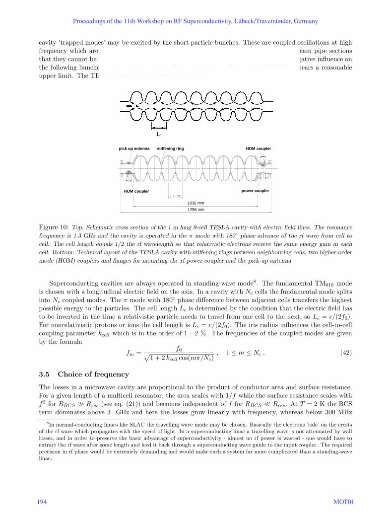
cavity ’trapped modes’ may be excited by the short particle bunches. These are coupled oscillations at highfrequency which are confined to the inner cells and have such a low amplitude in the beam pipe sectionsthat they cannot be extracted by a higher-order mode coupler. Trapped modes have a negative influence onthe following bunches and must be avoided. The number Nc = 9 chosen for TESLA appears a reasonableupper limit. The TESLA cavity [22] is shown in Fig. 10.

stiffening ring HOM couplerpick up antenna

HOM coupler power coupler

1036 mm

1256 mm

Figure 10: Top: Schematic cross section of the 1 m long 9-cell TESLA cavity with electric field lines. The resonance

frequency is 1.3 GHz and the cavity is operated in the π mode with 180 phase advance of the rf wave from cell to

cell. The cell length equals 1/2 the rf wavelength so that relativistic electrons recieve the same energy gain in each

cell. Bottom: Technical layout of the TESLA cavity with stiffening rings between neighbouring cells, two higher-order

mode (HOM) couplers and flanges for mounting the rf power coupler and the pick-up antenna.

Superconducting cavities are always operated in standing-wave mode8. The fundamental TM010 modeis chosen with a longitudinal electric field on the axis. In a cavity with Nc cells the fundamental mode splitsinto Nc coupled modes. The π mode with 180 phase difference between adjacent cells transfers the highestpossible energy to the particles. The cell length Lc is determined by the condition that the electric field hasto be inverted in the time a relativistic particle needs to travel from one cell to the next, so Lc = c/(2f0).For nonrelativistic protons or ions the cell length is Lc = v/(2f0). The iris radius influences the cell-to-cellcoupling parameter kcell which is in the order of 1 - 2 %. The frequencies of the coupled modes are givenby the formula

fm =f0√

1 + 2 kcell cos(mπ/Nc), 1 ≤ m ≤ Nc . (42)

3.5 Choice of frequency

The losses in a microwave cavity are proportional to the product of conductor area and surface resistance.For a given length of a multicell resonator, the area scales with 1/f while the surface resistance scales withf2 for RBCS Rres (see eq. (21)) and becomes independent of f for RBCS Rres. At T = 2 K the BCSterm dominates above 3 GHz and here the losses grow linearly with frequency, whereas below 300 MHz

8In normal-conducting linacs like SLAC the travelling wave mode may be chosen. Basically the electrons ’ride’ on the crestsof the rf wave which propagates with the speed of light. In a superconducting linac a travelling wave is not attenuated by walllosses, and in order to preserve the basic advantage of superconductivity - almost no rf power is wasted - one would have toextract the rf wave after some length and feed it back through a superconducting wave guide to the input coupler. The requiredprecision in rf phase would be extremely demanding and would make such a system far more complicated than a standing-wavelinac.


194 MOT01

the residual resistance dominates and the losses are proportional to 1/f . To minimize power dissipationin the cavity wall one should therefore select f in the range 300 MHz to 3 GHz. Cavities in the 350 to500 MHz regime are commonly used in electron-positron storage rings. Their large size is advantageous tosuppress wake field effects and losses from higher order modes. However, for a linac of several 10 km lengththe niobium and cryostat costs would be prohibitive for these bulky cavities, hence a higher frequency hasto be chosen. Considering material costs f = 3GHz might appear the optimum but there are compellingarguments for choosing about half this frequency.

• The wake fields generated by the short electron bunches depend on radius as 1/r2 for longitudinaland as 1/r3 for transverse wakes. Since the iris radius of a cavity is inversely proportional to itseigenfrequency, the wake field losses scale with the second resp. third power of the frequency. Beamemittance growth and beam-induced cryogenic losses are therefore much higher at 3 GHz.

• The f2 dependence of the BCS resistance makes a 3 GHz cavity thermally unstable at gradients above30 MV/m, hence choosing this frequency would preclude a possible upgrade of the TESLA collider to35 MV/m [10].

3.6 Heat conduction in niobium and heat transfer to the liquid helium

1 101

10

100

1000

8642 20

RRR = 500 RRR = 270

λ[W

/mK

]

T [K]

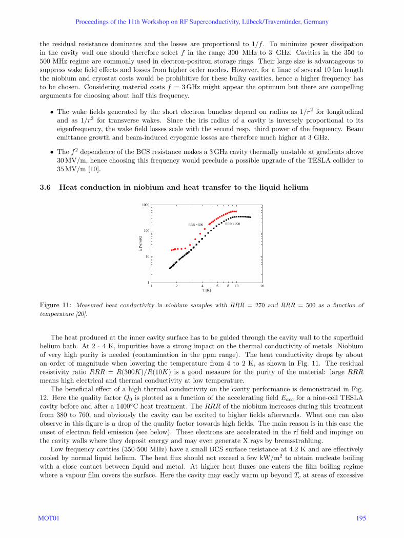
Figure 11: Measured heat conductivity in niobium samples with RRR = 270 and RRR = 500 as a function of

temperature [20].

The heat produced at the inner cavity surface has to be guided through the cavity wall to the superfluidhelium bath. At 2 - 4 K, impurities have a strong impact on the thermal conductivity of metals. Niobiumof very high purity is needed (contamination in the ppm range). The heat conductivity drops by aboutan order of magnitude when lowering the temperature from 4 to 2 K, as shown in Fig. 11. The residualresistivity ratio RRR = R(300K)/R(10K) is a good measure for the purity of the material: large RRRmeans high electrical and thermal conductivity at low temperature.

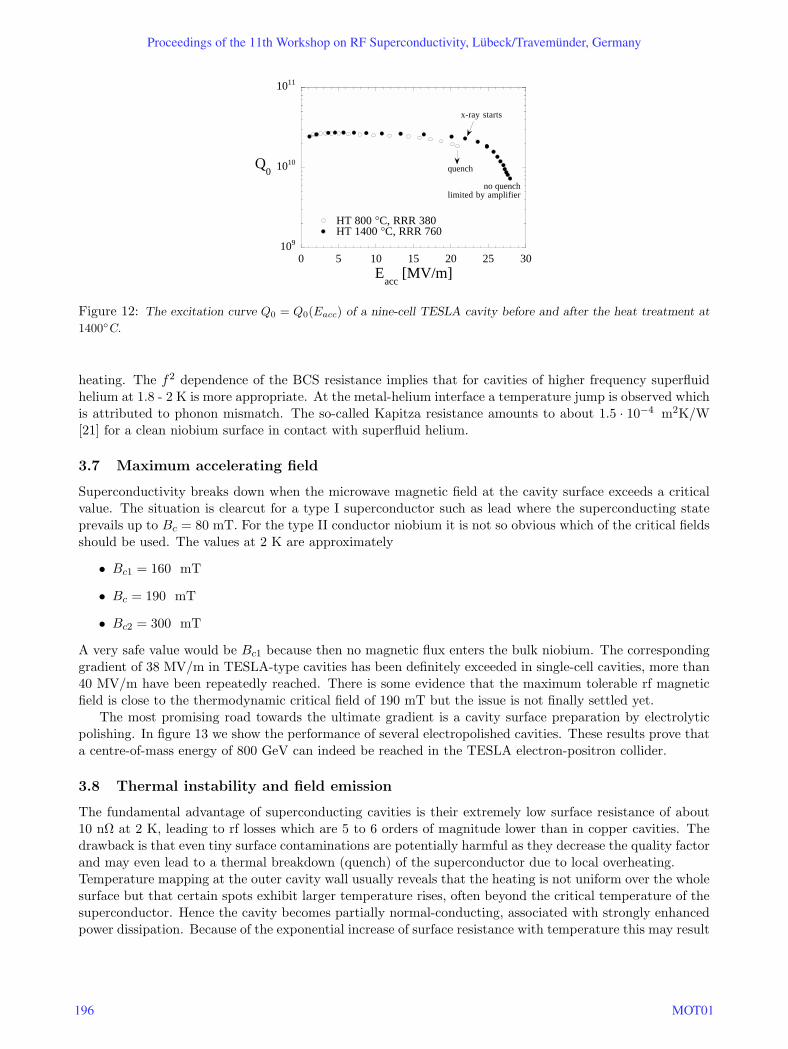
The beneficial effect of a high thermal conductivity on the cavity performance is demonstrated in Fig.12. Here the quality factor Q0 is plotted as a function of the accelerating field Eacc for a nine-cell TESLAcavity before and after a 1400C heat treatment. The RRR of the niobium increases during this treatmentfrom 380 to 760, and obviously the cavity can be excited to higher fields afterwards. What one can alsoobserve in this figure is a drop of the quality factor towards high fields. The main reason is in this case theonset of electron field emission (see below). These electrons are accelerated in the rf field and impinge onthe cavity walls where they deposit energy and may even generate X rays by bremsstrahlung.

Low frequency cavities (350-500 MHz) have a small BCS surface resistance at 4.2 K and are effectivelycooled by normal liquid helium. The heat flux should not exceed a few kW/m2 to obtain nucleate boilingwith a close contact between liquid and metal. At higher heat fluxes one enters the film boiling regimewhere a vapour film covers the surface. Here the cavity may easily warm up beyond Tc at areas of excessive


MOT01 195

109

1010

1011

0 5 10 15 20 25 30

HT 800 °C, RRR 380HT 1400 °C, RRR 760

Q0

Eacc

[MV/m]

quench

no quenchlimited by amplifier

x-ray starts

Figure 12: The excitation curve Q0 = Q0(Eacc) of a nine-cell TESLA cavity before and after the heat treatment at

1400C.

heating. The f2 dependence of the BCS resistance implies that for cavities of higher frequency superfluidhelium at 1.8 - 2 K is more appropriate. At the metal-helium interface a temperature jump is observed whichis attributed to phonon mismatch. The so-called Kapitza resistance amounts to about 1.5 · 10−4 m2K/W[21] for a clean niobium surface in contact with superfluid helium.

3.7 Maximum accelerating field

Superconductivity breaks down when the microwave magnetic field at the cavity surface exceeds a criticalvalue. The situation is clearcut for a type I superconductor such as lead where the superconducting stateprevails up to Bc = 80 mT. For the type II conductor niobium it is not so obvious which of the critical fieldsshould be used. The values at 2 K are approximately

• Bc1 = 160 mT

• Bc = 190 mT

• Bc2 = 300 mT

A very safe value would be Bc1 because then no magnetic flux enters the bulk niobium. The correspondinggradient of 38 MV/m in TESLA-type cavities has been definitely exceeded in single-cell cavities, more than40 MV/m have been repeatedly reached. There is some evidence that the maximum tolerable rf magneticfield is close to the thermodynamic critical field of 190 mT but the issue is not finally settled yet.

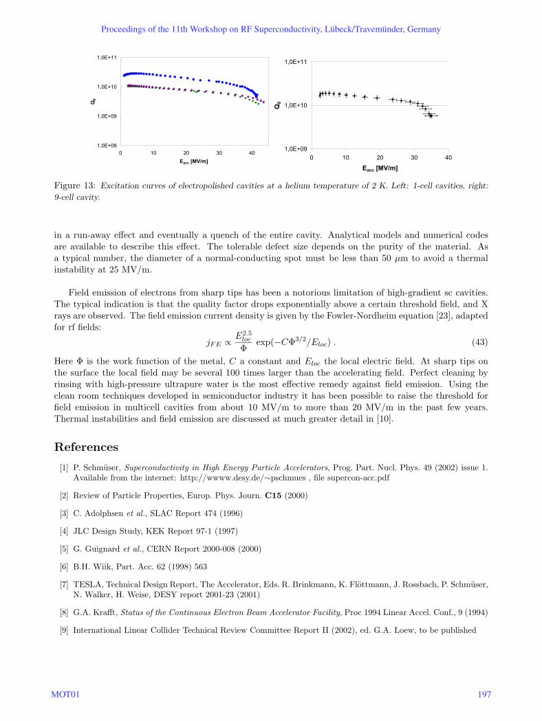
The most promising road towards the ultimate gradient is a cavity surface preparation by electrolyticpolishing. In figure 13 we show the performance of several electropolished cavities. These results prove thata centre-of-mass energy of 800 GeV can indeed be reached in the TESLA electron-positron collider.

3.8 Thermal instability and field emission

The fundamental advantage of superconducting cavities is their extremely low surface resistance of about10 nΩ at 2 K, leading to rf losses which are 5 to 6 orders of magnitude lower than in copper cavities. Thedrawback is that even tiny surface contaminations are potentially harmful as they decrease the quality factorand may even lead to a thermal breakdown (quench) of the superconductor due to local overheating.Temperature mapping at the outer cavity wall usually reveals that the heating is not uniform over the wholesurface but that certain spots exhibit larger temperature rises, often beyond the critical temperature of thesuperconductor. Hence the cavity becomes partially normal-conducting, associated with strongly enhancedpower dissipation. Because of the exponential increase of surface resistance with temperature this may result


196 MOT01

1,0E+08

1,0E+09

1,0E+10

1,0E+11

0 10 20 30 40Eacc [MV/m]

Q0

1,0E+09

1,0E+10

1,0E+11

0 10 20 30 40

Eacc [MV/m]

Q0

Figure 13: Excitation curves of electropolished cavities at a helium temperature of 2 K. Left: 1-cell cavities, right:

9-cell cavity.

in a run-away effect and eventually a quench of the entire cavity. Analytical models and numerical codesare available to describe this effect. The tolerable defect size depends on the purity of the material. Asa typical number, the diameter of a normal-conducting spot must be less than 50 µm to avoid a thermalinstability at 25 MV/m.

Field emission of electrons from sharp tips has been a notorious limitation of high-gradient sc cavities.The typical indication is that the quality factor drops exponentially above a certain threshold field, and Xrays are observed. The field emission current density is given by the Fowler-Nordheim equation [23], adaptedfor rf fields:

jFE ∝E2.5

loc

Φexp(−CΦ3/2/Eloc) . (43)

Here Φ is the work function of the metal, C a constant and Eloc the local electric field. At sharp tips onthe surface the local field may be several 100 times larger than the accelerating field. Perfect cleaning byrinsing with high-pressure ultrapure water is the most effective remedy against field emission. Using theclean room techniques developed in semiconductor industry it has been possible to raise the threshold forfield emission in multicell cavities from about 10 MV/m to more than 20 MV/m in the past few years.Thermal instabilities and field emission are discussed at much greater detail in [10].

References

[1] P. Schmuser, Superconductivity in High Energy Particle Accelerators, Prog. Part. Nucl. Phys. 49 (2002) issue 1.Available from the internet: http://wwww.desy.de/∼pschmues , file supercon-acc.pdf

[2] Review of Particle Properties, Europ. Phys. Journ. C15 (2000)

[3] C. Adolphsen et al., SLAC Report 474 (1996)

[4] JLC Design Study, KEK Report 97-1 (1997)

[5] G. Guignard et al., CERN Report 2000-008 (2000)

[6] B.H. Wiik, Part. Acc. 62 (1998) 563

[7] TESLA, Technical Design Report, The Accelerator, Eds. R. Brinkmann, K. Flottmann, J. Rossbach, P. Schmuser,N. Walker, H. Weise, DESY report 2001-23 (2001)

[8] G.A. Krafft, Status of the Continuous Electron Beam Accelerator Facility, Proc 1994 Linear Accel. Conf., 9 (1994)

[9] International Linear Collider Technical Review Committee Report II (2002), ed. G.A. Loew, to be published


MOT01 197

[10] H. Padamsee, J. Knobloch and T. Hays, RF Superconductivity for Accelerators, John Wiley, New York 1998.

[11] H. Piel in: Proc. of the 1988 CERN Accelerator School Superconductivity in Particle Accelerators, CERN report89-04 (1989)

[12] D.C. Larbalestier and P.J. Lee, Proc. PAC99, New York (1999) 177

[13] W. Buckel, Supraleitung, VCH Verlagsgesellschaft, Weinheim 1990

[14] D.R. Tilley and J. Tilley, Superfluidity and Superconductivity, Institute of Physics Publishing Ltd, Bristol 1990

[15] E.W. Collings et al., Adv. Cryog. Eng. 36 (1990) 169

[16] G. Muller, Proc. 3rd Workshop on RF Superconductivity, ed. K.W. Shepard, Argonne, USA (1988), p. 331

[17] B. Bonin, CERN Accelerator School Superconductivity in Particle Accelerators, CERN 96-03, ed. S. Turner,Hamburg (1995)

[18] J. Halbritter, Z. Physik 238 (1970) 466

[19] C. Benvenuti et al., Proc. PAC91, San Francisco (1991), p. 1023.

[20] T. Schilcher, TESLA-Report, TESLA 95-12, DESY (1995)

[21] A. Boucheffa et al., Proc. 7th Workshop on RF Superconductivity, ed. B. Bonin, Gif-sur-Yvette, France (1995),p. 659

[22] B. Aune et al., Phys. Rev. Spec. Top. Acc. Beams PRSTAB 3 (2000) 092001

[23] R.H. Fowler and L. Nordheim, Proc. of the Roy. Soc. A 119, 173 and Math. Phys. Sci. 119 (1928) 173.


198 MOT01

Documents

Basic Principles of RF Superconductivity and ... · PDF fileBasic Principles of RF Superconductivity and Superconducting Cavities 1 ... The vanishing electrical resistance of ... machine