Basic principles of RF superconductivity and ... · PDF file1.1 Advantages and limitations of superconductor technology in accelerators The vanishing electrical resistance ... needed

Basic principles of RF superconductivity and superconducting cavities∗

P. SchmuserInstitut fur Experimentalphysik, Universitat Hamburg, Germany

AbstractThe basics of superconductivity are outlined with special emphasis on the fea-tures which are relevant for the application of superconductors in radio fre-quency cavities for particle acceleration. For a cylindrical resonator (“pill boxcavity”) the electromagnetic field in the cavity and important parameters suchas resonance frequency, quality factor and shunt impedance are calculated ana-lytically. The design and performance of practical cavities is shortly addressed.

1 Introduction1.1 Advantages and limitations of superconductor technology in acceleratorsThe vanishing electrical resistance of superconducting coils as well as their ability to provide magneticfields far beyond those of saturated iron is the main motivation for using superconducting (sc) magnetsin all new large proton, antiproton and heavy ion accelerators1. Superconductivity does not only openthe way to much higher particle energies but at the same time leads to a substantial reduction of oper-ating costs. In the normal-conducting Super Proton Synchrotron SPS at CERN a power of 52 MW isneeded to operate the machine at an energy of 315 GeV while at HERA a cryogenic plant with 6 MWelectrical power consumption is sufficient to provide the cooling of the superconducting magnets witha stored proton beam of 920 GeV. Hadron energies in the TeV regime are practically inaccessible withstandard magnet technology. Another important application of superconducting materials is in the largeexperiments at hadron or lepton colliders where superconducting detector magnets are far superior tonormal magnets.

In the case of accelerating cavities the advantage of superconductors is not at all that obvious. Infact, three of the proposed linear electron positron colliders are based on copper acceleration structures:the ‘Next Linear Collider’ NLC [3] at Stanford, the ‘Japanese Linear Collider’ JLC [4] at Tsukuba,and the ‘Compact Linear Collider’ CLIC [5] at CERN, while only the international TESLA project[6, 7] uses sc niobium cavities. The traditional arguments against superconductor technology in linearcolliders have been the low accelerating fields achieved in sc cavities and the high cost of cryogenicequipment. Superconducting cavities face a strong physical limitation: the microwave magnetic fieldmust stay below the critical field of the superconductor. For the best superconductor for cavities, niobium,this corresponds to a maximum accelerating field of about 45 MV/m while normal-conducting cavitiesoperating at high frequency (above 5 GHz) should in principle be able to reach 100 MV/m or more. Inpractice, however, sc cavities were often found to be limited at much lower fields of some 5 MV/m andhence were totally non-competitive for a linear collider. Great progress was achieved with the 340 five-cell cavities of the Continuous Electron Beam Accelerator Facility CEBAF [8] at Jefferson Laboratoryin Virginia, USA. These 1.5 GHz niobium cavities were developed at Cornell University and producedby industry. They exceeded the design gradient of 5 MV/m and achieved 8.4 MV/m after installation inthe accelerator (in several specially prepared cavities even 15-20 MV/m were reached). Building uponthe CEBAF experience the intensive R&D of the TESLA collaboration has succeeded in raising theaccelerating field in multicell cavities to more than 25 MV/m. There is a realistic chance to reach even35 MV/m, and to reduce substantially the cost for the cryogenic installation.

∗Adapted from a review article [1].1The parameters of high energy lepton and hadron colliders are summarized in [2].

183

While superconducting magnets operated with direct current are free of energy dissipation, this isnot the case in microwave cavities. The non-superconducting electrons (see sect. 2) experience forcedoscillations in the time-varying magnetic field and dissipate power in the material. Although the resultingheat deposition is many orders of magnitude smaller than in copper cavities it constitutes a significantheat load on the refrigeration system. As a rule of thumb, 1 W of heat deposited at 2 K requires almost1 kW of primary ac power in the refrigerator. Nevertheless, there is now a worldwide consensus thatthe overall efficiency for converting primary electric power into beam power is about a factor two higherfor a superconducting than for a normal-conducting linear collider with optimized parameters in eithercase [9]. Another definite advantage of a superconducting collider is the low resonance frequency of thecavities that can be chosen (1.3 GHz in TESLA). The longitudinal (transverse) wake fields generatedby the ultrashort electron bunches upon passing the cavities scale with the second (third) power of thefrequency and are hence much smaller in TESLA than in NLC (f = 11 GHz). The wake fields may havea negative impact on the beam emittance (the area occupied in phase space) and on the luminosity of thecollider.

1.2 Characteristic properties of superconducting cavitiesThe fundamental advantage of superconducting niobium cavities is the extremely low surface resistanceof a few nano-ohms at 2 Kelvin as compared to several milli-ohms in copper cavities. The qualityfactor Q0 (2π times the ratio of stored energy to energy loss per cycle) is inversely proportional to thesurface resistance and may exceed 1010. Only a tiny fraction of the incident radio frequency (rf) poweris dissipated in the cavity walls, the lion’s share is transferred to the beam. The physical limitation of asc resonator is given by the requirement that the rf magnetic field at the inner surface has to stay belowthe critical field of the superconductor (about 190 mT for niobium), corresponding to an acceleratingfield of Eacc = 45 MV/m. In principle the quality factor should stay constant when approaching thisfundamental superconductor limit but in practice the curve Q0 = Q0(Eacc) ends at considerably lowervalues, often accompanied with a strong decrease of Q0 towards the highest gradient reached in thecavity. The main reasons for the performance degradation are excessive heating caused by impuritieson the inner surface or by field emission of electrons. The cavity becomes partially normal-conducting,associated with strongly enhanced power dissipation. Because of the exponential increase of surfaceresistance with temperature this may result in a run-away effect and eventually a quench of the entirecavity.

Field emission of electrons from sharp tips is the most severe limitation in high-gradient superconductingcavities. Small particles on the cavity surface act as field emitters. By applying the clean room techniquesdeveloped in semiconductor industry it has been possible to raise the threshold for field emission inmulticell cavities from about 10 MV/m to more than 20 MV/m in the past few years. The preparation ofa smooth and almost mirror-like surface by electrolytic polishing is another important improvement.

A detailed description of sc cavities is found in [10].

2 Basics of superconductivityThe unusual features of superconducting magnets and cavities are closely linked to the physical proper-ties of the superconductor itself. For this reason a basic understanding of superconductivity is indispens-able for the design, construction and operation of superconducting accelerator components. Only thetraditional ‘low-temperature’ superconductors are treated since up to date the use of ‘high-temperature’ceramic superconductors in these devices is rather limited [11, 12]. For more comprehensive presenta-tions I refer to the excellent text books by W. Buckel [13] and by D.R. Tilley and J. Tilley [14].

2

P. SCHMUSER

184

2.1 OverviewSuperconductivity — the infinitely high conductivity below a ‘critical temperature‘ Tc — is observed ina large variety of materials but, remarkably, not in some of the best normal conductors like copper, silverand gold, except at very high pressures. This is illustrated in Fig. 1 where the resistivity of copper, tin andthe ‘high-temperature‘ superconductor YBa2Cu3O7 is sketched as a function of temperature. Table 1 listssome important superconductors together with their critical temperatures at vanishing magnetic field.

Fig. 1: The low-temperature resistivity of copper, tin and YBa2Cu3O7.

Table 1: Critical temperature Tc in K of selected superconducting materials for vanishing magnetic field.

Al Hg Sn Pb Nb Ti NbTi Nb3Sn

1.14 4.15 3.72 7.9 9.2 0.4 9.4 18

There is an intimate relation between superconductivity and magnetic fields. W. Meissner and R.Ochsenfeld discovered in 1933 that a superconducting element like lead expels a weak magnetic fieldfrom its interior when cooled below Tc, while in stronger fields superconductivity breaks down andthe material goes to the normal state. The spontaneous exclusion of magnetic fields upon crossing Tc

cannot be explained in terms of the Maxwell equations of classical electrodynamics and indeed turnedout to be of quantum-theoretical origin. In 1935 H. and F. London proposed an equation which offereda phenomenological explanation of the field exclusion. The London equation relates the supercurrentdensity Js to the magnetic field:

~∇× ~Js = −nse2

me

~B (1)

where ns is the density of the super-electrons. In combination with the Maxwell equation ~∇× ~B = µ0~Js

we get the following equation for the magnetic field in a superconductor

∇2 ~B − µ0nse2

me

~B = 0 . (2)

For a simple geometry, namely the boundary between a superconducting half space and vacuum, andwith a magnetic field parallel to the surface, Eq. (2) reads

d2By

dx2− 1

λ2L

By = 0 with λL =√

me

µ0nse2. (3)

Here we have introduced a very important superconductor parameter, the London penetration depth λL.The solution of the differential equation is

By(x) = B0 exp(−x/λL) . (4)

3

BASIC PRINCIPLES OF RF SUPERCONDUCTIVITY AND SUPERCONDUCTING CAVITIES

185

So the magnetic field does not abruptly drop to zero at the superconductor surface but penetrates into thematerial with exponential attenuation (Fig. 2). For typical material parameters the penetration depth isquite small, namely 20–50 nm. In the bulk of a thick superconductor the magnetic field vanishes whichis just the Meissner-Ochsenfeld effect.

The justification of the London equation remained obscure until the advent of the microscopictheory of superconductivity by Bardeen, Cooper and Schrieffer in 1957. The BCS theory is based on theassumption that the supercurrent is not carried by single electrons but rather by pairs of electrons of op-posite momenta and spins, the so-called Cooper pairs. The London penetration depth remains invariantunder the replacements ns → nc = ns/2, e → 2e and me → mc = 2me. The BCS theory revolu-

Fig. 2: The exponential drop of the magnetic field and the rise of the Cooper-pair density at a boundary between anormal and a superconductor.

tionized our understanding of superconductivity. All Cooper pairs occupy a single quantum state, theBCS ground state, whose energy is separated from the single-electron states by a temperature dependentenergy gap Eg = 2∆(T ). The critical temperature is related to the energy gap at T = 0 by

1.76 kBTc = ∆(0) . (5)

Here kB = 1.38 · 10−23 J/K is the Boltzmann constant. The magnetic flux through a superconductingring is found to be quantized, the smallest unit being the elementary flux quantum

Φ0 =h

2e= 2.07 · 10−15 Vs . (6)

These and many other predictions of the BCS theory, like the temperature dependence of the energy gapand the existence of quantum interference phenomena, have been confirmed by experiment and oftenfound practical application.

A discovery of enormous practical consequences was the finding that there exist two types ofsuperconductors with rather different response to magnetic fields. The elements lead, mercury, tin,aluminium and others are called ’type I‘ superconductors. They do not admit a magnetic field in thebulk material and are in the superconducting state provided the applied field stays below a critical fieldHc (Bc = µ0Hc is usually less than 0.1 Tesla). All superconducting alloys like lead-indium, niobium-titanium, niobium-tin and also the element niobium belong to the large class of ’type II‘ superconductors.They are characterized by two critical fields, Hc1 and Hc2. Below Hc1 these substances are in the Meiss-ner phase with complete field expulsion while in the range Hc1 < H < Hc2 they enter the mixed phasein which the magnetic field pierces the bulk material in the form of flux tubes. Many of these materialsremain superconductive up to much higher fields (10 Tesla or more).

2.2 Energy balance in a magnetic fieldA material like lead makes a phase transition from the normal to the superconducting state when it iscooled below Tc and when the magnetic field is less than Hc(T ). This is a phase transition comparable to

4

P. SCHMUSER

186

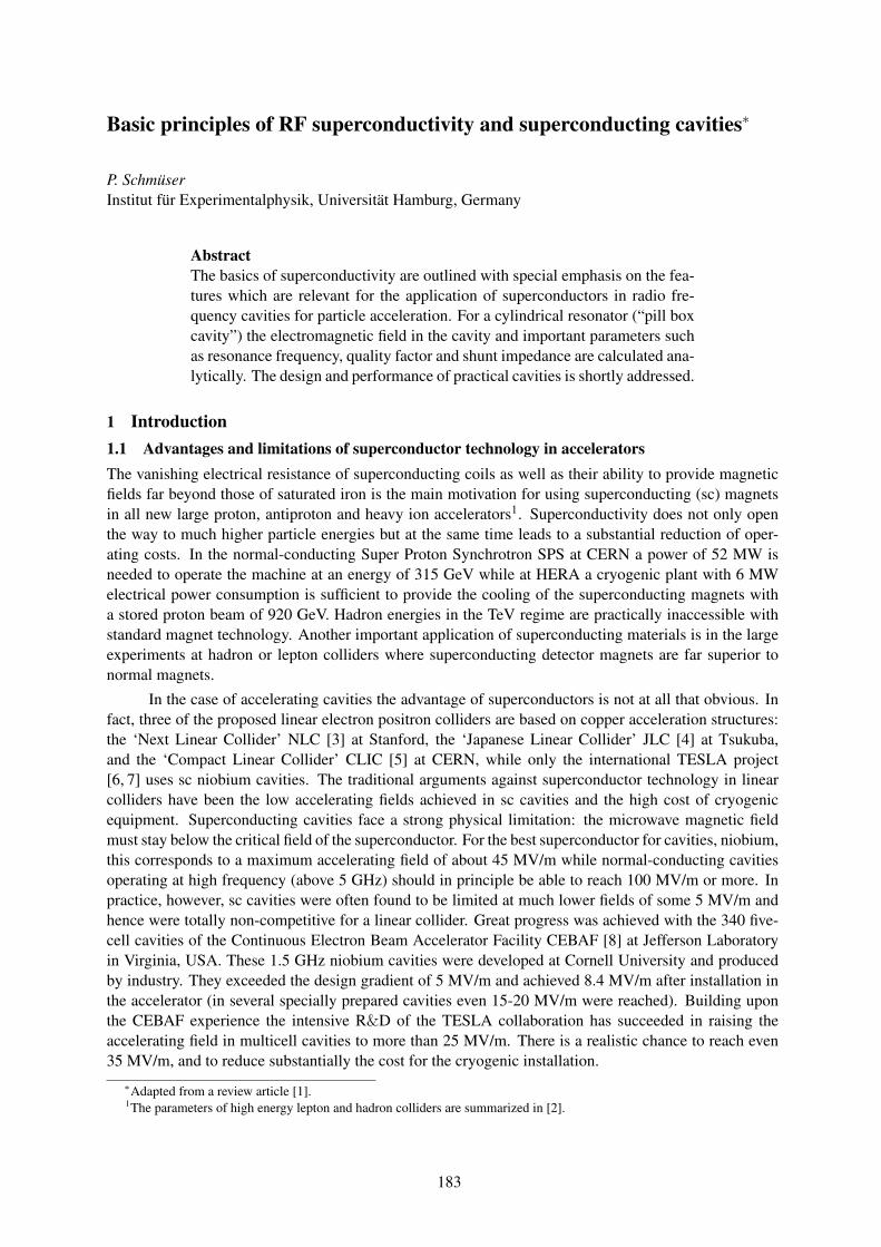
the transition from water to ice below 0C. Phase transitions take place when the new state is energeticallyfavoured. The relevant thermodynamic energy is here the so-called Gibbs free energy G. Free energieshave been measured for a variety of materials. For temperatures T < Tc they are found to be lower inthe superconducting than in the normal state while Gsup approaches Gnorm in the limit T → Tc, see Fig.3a. What is now the impact of a magnetic field on the energy balance? A magnetic field has an energydensity µ0/2 ·H2, and according to the Meissner-Ochsenfeld effect the magnetic energy must be pushedout of the material when it enters the superconducting state. Hence the free energy per unit volume inthe superconducting state increases quadratically with the applied field:

Gsup(H) = Gsup(0) +µ0

2H2 . (7)

The normal-state energy remains unaffected. The material stays superconductive as long as Gsup(H) <Gnorm. Equation (7) implies the existence of a maximum tolerable field, the ‘critical field’, above whichsuperconductivity breaks down. It is defined by the condition that the free energies in the superconductingand in the normal state be equal

Gsup(Hc) = Gnorm ⇒ µ0

2H2

c = Gnorm −Gsup(0) . (8)

Figure 3b illustrates what we have said. For H > Hc the normal phase has a lower energy, so the materialgoes to the normal state. Equation (8) is also meaningful for type II superconductors and defines in thiscase the thermodynamic critical field which lies between Hc1 and Hc2. The quantity µ0/2 · H2

c =

Fig. 3: (a) Free energy of aluminium in the normal and superconducting state as a function of T (after N.E.Phillips). The normal state is achieved by applying a magnetic field larger than Bc. (b) Schematic sketch of thefree energies Gnorm and Gsup as a function of the applied magnetic field B = µ0H .

Gnorm −Gsup(0) can be interpreted as the Cooper-pair condensation energy per unit volume.

2.3 Coherence length and distinction between type I and type II superconductorsIn very thin sheets of superconductor (thickness < λL) the magnetic field does not drop to zero at thecentre. Consequently less magnetic energy needs to be expelled which implies that the critical fieldof a thin sheet may be much larger than the Hc of a thick slab. From this point of view it might appearenergetically favourable for a thick slab to subdivide itself into an alternating sequence of thin normal andsuperconducting slices. The magnetic energy is indeed lowered that way but there is another energy tobe taken into consideration, namely the energy required to create the normal-superconductor interfaces.At the boundary between the normal and the superconducting phase the density nc of the super-currentcarriers (the Cooper pairs) does not jump abruptly from zero to its value in the bulk but rises smoothlyover a finite length ξ, called coherence length, see Fig. 2.

5


187

The relative size of the London penetration depth λL and the coherence length ξ decides whethera material is a type I or a type II superconductor. Creation of a boundary means a loss of Cooper-paircondensation energy in a thickness ξ but a gain of magnetic energy in a thickness λL. There is a netenergy gain if λL > ξ. So a subdivision of the superconductor into an alternating sequence of thinnormal and superconducting slices is energetically favourable if the London penetration depth exceedsthe coherence length.

A more refined treatment is provided by the Ginzburg-Landau theory (see e.g. [14]). Here oneintroduces the Ginzburg-Landau parameter

κ = λL/ξ . (9)

The criterion for type I or II superconductivity is found to be

type I: κ < 1/√

2type II: κ > 1/

√2.

Table 2 lists the penetration depths and coherence lengths of some important superconducting elements.Niobium is a type II conductor but close to the border to type I, while indium, lead and tin are clearly inthe type I class. The coherence length ξ is proportional to the mean free path of the conduction electrons

Table 2: Penetration depths and coherence lengths of important superconducting elements.

material In Pb Sn Nb

λL [nm] 24 32 ≈ 30 32

ξ [nm] 360 510 ≈ 170 39

in the metal. In alloys the mean free path is generally much shorter than in pure metals hence alloys arealways type II conductors.

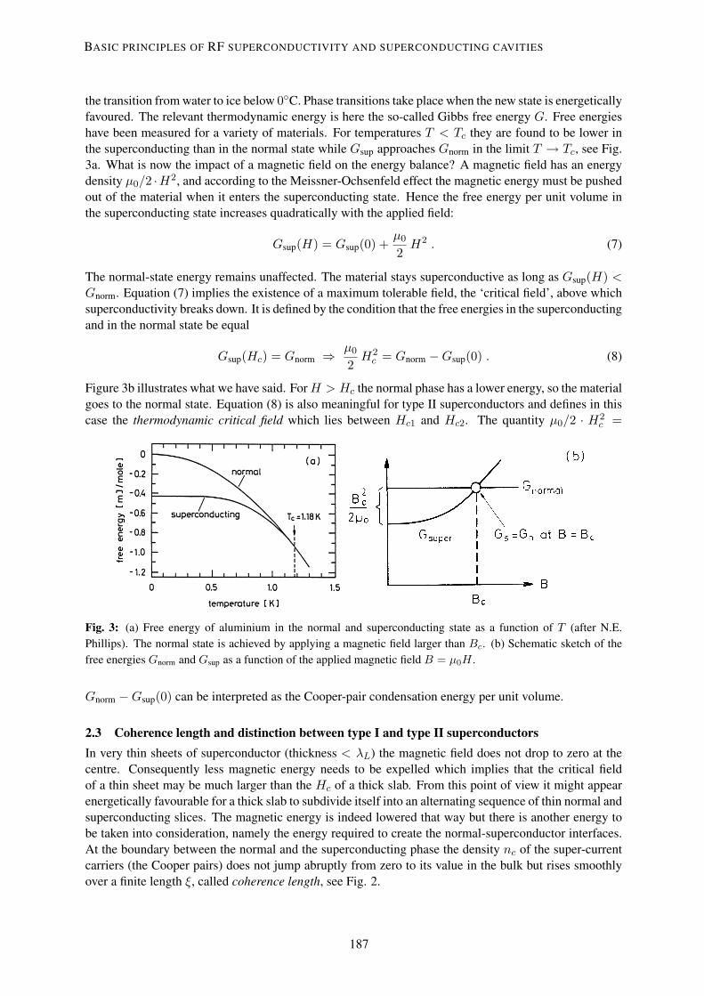
In reality a type II superconductor is not subdivided into thin slices but the field penetrates thesample in the form of flux tubes which arrange themselves in a triangular pattern which can be madevisible by evaporating iron atoms onto a superconductor surface sticking out of the liquid helium. Thefluxoid pattern shown in Fig. 4a proves beyond any doubt that niobium is indeed a type II superconductor.Each flux tube or fluxoid contains one elementary flux quantum Φ0 which is surrounded by a Cooper-pair vortex current. The centre of a fluxoid is normal-conducting and covers an area of roughly πξ2.When we apply an external field H , fluxoids keep moving into the specimen until their average magnetic

flux density is identical to B = µ0H . The fluxoid spacing in the triangular lattice d =√

2Φ0/(√

3B)amounts to 20 nm at 6 Tesla. The upper critical field is reached when the current vortices of the fluxoidsstart touching each other at which point superconductivity breaks down. In the Ginzburg-Landau theorythe upper critical field is given by

Bc2 =√

2 κ Bc =Φ0

2πξ2. (10)

For niobium-titanium with an upper critical field Bc2 = 14 T this formula yields ξ = 5 nm. Thecoherence length is larger than the typical width of a grain boundary in NbTi which means that thesupercurrent can freely move from grain to grain. In high-Tc superconductors the coherence length isoften shorter than the grain boundary width, and then current flow from one grain to the next is stronglyimpeded.

6

P. SCHMUSER

188

2.4 Flux flow resistance and flux pinningFor application in accelerator magnets a superconducting wire must be able to carry a large current in thepresence of a field of 5 – 10 Tesla. Type I superconductors are definitely ruled out because their criticalfield is far too low (below 0.1 Tesla). Type II conductors appear promising at first sight: they featurelarge upper critical fields, and high currents are permitted to flow in the bulk material. However there isthe problem of flux flow resistance. A current flowing through an ideal type II superconductor, which isexposed to a magnetic field, exerts a Lorentz force on the flux lines and causes them to move through thespecimen, see Fig. 4b. This is a viscous motion and leads to heat generation. So although the currentitself flows without dissipation the sample acts as if it had an Ohmic resistance. The statement is evenformally correct. The moving fluxoids represent a moving magnetic field which, according to theory ofspecial relativity, is equivalent to an electric field ~Eequiv = ~B × ~v/c2 . It is easy to see that ~Eequiv and ~Jpoint in the same direction just like in a normal resistor. To obtain useful wires for magnet coils flux flow

Fig. 4: (a) Fluxoid pattern in niobium (courtesy U. Essmann). The distance between adjacent flux tubes is 0.2 µm.(b) Fluxoid motion in a current-carrying type II superconductor.

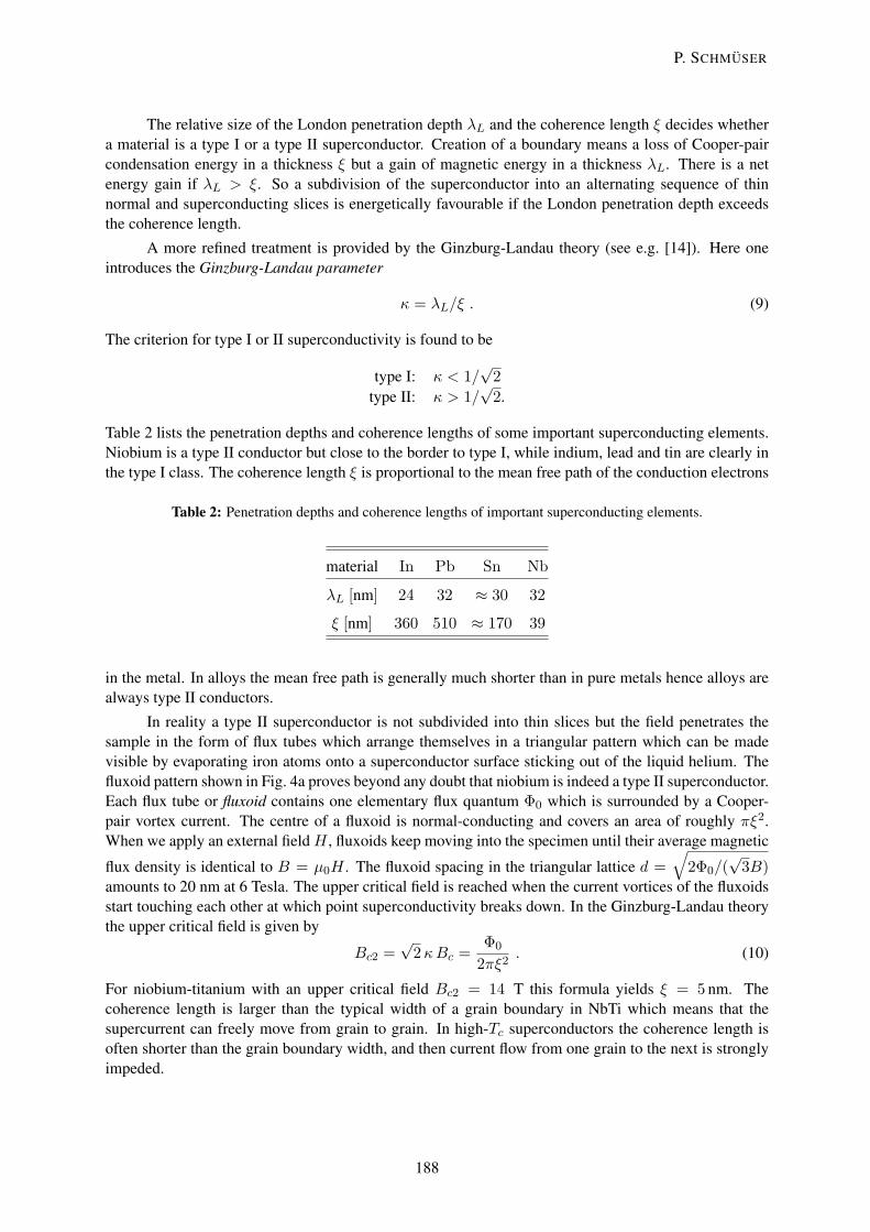
has to be prevented by capturing the fluxoids at pinning centres. These are defects or impurities in theregular crystal lattice. The most important pinning centres in niobium-titanium are normal-conductingtitanium precipitates in the so-called α phase whose size is in the range of the fluxoid spacing (≈ 10 nmat 6 Tesla). Figure 5 shows a microscopic picture of a conductor with very high current density (3700A/mm2 at 5 T and 4.2 K).

Fig. 5: Micrograph of NbTi. The α-titanium precipitates appear as lighter strips. The area covered is 840 nm wideand 525 nm high. Courtesy P.J. Lee and D.C. Larbalestier.

A type II superconductor with strong pinning is called a hard superconductor. Hard superconduc-tors are very well suited for high-field magnets, they permit dissipationless current flow in high magneticfields. There is a penalty, however: these conductors exhibit a strong magnetic hysteresis which is theorigin of the very annoying ’persistent-current‘ multipoles in superconducting accelerator magnets.

7


189

2.5 Magnetization of a hard superconductorA type I superconductor shows a reversible response2 to a varying external magnetic field H . Themagnetization is given by the straight line M(H) = −H for 0 < H < Hc and then drops to zero. Anideal type II conductor without any flux pinning should also react reversibly. A hard superconductor, onthe other hand, is only reversible in the Meissner phase because then no magnetic field enters the bulk,so no flux pinning can happen. If the field is raised beyond Hc1 magnetic flux enters the sample andis captured at pinning centres. When the field is reduced again these flux lines remain bound and thespecimen keeps a frozen-in magnetization even for vanishing external field. One has to invert the fieldpolarity to achieve M = 0 but the initial state (H = 0 and no captured flux in the bulk material) canonly be recovered by warming up the specimen to destroy superconductivity and release all pinned fluxquanta, and by cooling down again.

A typical hysteresis curve is shown in Fig. 6. There is a close resemblence with the hysteresisin iron except for the sign: the magnetization in a superconductor is opposed to the magnetizing fieldbecause the physical mechanism is diamagnetism. The magnetic hysteresis is associated with energy

Fig. 6: Measured magnetization M of a multifilamentary niobium-titanium conductor [15]. Shown is the initialexcitation, starting at B = µ0H = 0 and M = 0, and the magnetic hysteresis for an external field B varyingbetween +0.5 T and -0.5 T. Note that the hysteresis curve is not exactly symmetric with respect to the horizontalaxis. The slight asymmetry is due to surface currents (Meissner-Ochsenfeld effect) whose magnetic moment isalways opposed to the applied field.

dissipation. When a hard superconductor is exposed to a time-varying field and undergoes a cycle likethe loop in Fig. 6, the energy loss is given by the integral

Qhyst =∮

µ0M(H)dH . (11)

It is equal to the area enclosed by the loop. This energy must be provided by the power supply of thefield-generating magnet and is transformed into heat in the superconductor when magnetic flux quantaare moved in and out of the specimen.

2.6 Critical current densityFor a hard superconductor, not only temperature T and magnetic field H have to be specified but alsocurrent density J . The material can be conveniently characterized by its critical surface in a (T, H, J)coordinate system. For the most important conductor used in magnets, niobium-titanium, this surface is

2This statement applies only for long cylindral or elliptical samples oriented parallel to the field.

8

P. SCHMUSER

190

depicted in Fig. 7. Superconductivity prevails everywhere below the surface and normal conductivityabove it. A hard superconductor is not exactly free of any resistance. The critical current density (at agiven temperature and field) is usually defined by the criterion that the resistivity be ρ = ρc = 10−14 Ωm.In the vicinity of this point the resistivity is a very steep function of current density. It can be parametrisedwith a power law

ρ(J) = ρc

(J

Jc

)n

. (12)

The exponent n is a quality index which may be as large as 50 for a good multifilamentary NbTi conduc-tor.

Fig. 7: Sketch of the critical surface of NbTi. Also indicated are the regions where pure niobium and pure titaniumare superconducting. The critical surface has been truncated in the regime of very low temperatures and fieldswhere only sparse data are available.

2.7 Superconductors in microwave fieldsSuperconductivity in microwave fields is not treated adequately in standard text books. For this reasonI present in this section a simplified explanation of the important concepts. A similar treatment can befound in [10]. Superconductors are free from energy dissipation in direct-current (dc) applications, butthis is no longer true for alternating currents (ac) and particularly not in microwave fields. The reasonis that the high-frequency magnetic field penetrates a thin surface layer and induces oscillations of theelectrons which are not bound in Cooper pairs. The power dissipation caused by the motion of theunpaired electrons can be characterized by a surface resistance. In copper cavities the surface resistanceis given by (see sect. 3.2.3)

Rsurf =1δσ

(13)

where δ is the skin depth and σ the conductivity of the metal.

The response of a superconductor to an ac field can be understood in the framework of the two-fluid model 3. An ac current in a superconductor is carried by Cooper pairs (the superfluid component)as well as by unpaired electrons (the normal component). Let us study the response to a periodic electricfield. The normal current obeys Ohm’s law

Jn = σn E0 exp(−iωt) (14)3A similar model is used to explain the peculiar properties of liquid helium below 2.17 K.

9


191

while the Cooper pairs receive an acceleration mc vc = −2eE0 exp(−iωt), so the supercurrent densitybecomes

Js = inc 2 e2

meωE0 exp(−iωt) . (15)

If we write for the total current density

J = Jn + Js = σE0 exp(−iωt) (16)

we get a complex conductivity:

σ = σn + iσs with σs =2 nce

2

me ω=

1µ0λ2

L ω. (17)

We know already that the rf magnetic field penetrates a superconductor much less than a normal conduc-tor, namely only to a depth λL. The surface resistance is the real part of the complex surface impedance

Rsurf = Re

(1

λL(σn + iσs)

)=

1λL· σn

σ2n + σ2

s

. (18)

Since σ2n σ2

s at microwave frequencies one can disregard σ2n in the denominator and obtains Rsurf ∝

σn/(λLσ2s). So we arrive at the surprising result that the microwave surface resistance is proportional to

the normal-state conductivity.

The conductivity of a normal metal is given by the classic Drude expression

σn =nne2`

mevF(19)

where nn is the density of the unpaired electrons, ` their mean free path and vF the Fermi velocity. Thenormal electrons are created by thermal breakup of Cooper pairs. There is an energy gap Eg = 2∆(T )between the BCS ground state and the free electron states. By analogy with the conductivity of anintrinsic (undoped) semiconductor we get nn ∝ exp(−Eg/(2kBT )) and hence

σn ∝ ` exp(−∆(T )/(kBT )) . (20)

Using 1/σs = µ0λ2Lω and ∆(T ) ≈ ∆(0) = 1.76kBTc we finally obtain for the BCS surface resistance

RBCS ∝ λ3L ω2 ` exp(−1.76 Tc/T ) . (21)

This formula displays two important aspects of microwave superconductivity: the surface resistancedepends exponentially on temperature, and it is proportional to the square of the rf frequency.

3 Design principles and properties of superconducting cavities3.1 Choice of superconductorIn principle the critical temperature of the superconductor should be as high as possible. However, cop-per cavities coated with a high-Tc superconductor layer have shown unsatisfactory performance [11],therefore the helium-cooled low-Tc superconductors are applied. In contrast to magnets were hard su-perconductors with large upper critical field (10–20 T) are needed, the superconductor in microwaveapplications is not limited by the upper critical field but rather by the thermodynamic critical field (orpossibly the ‘superheating field’) which is well below 0.5 T for all known superconducting elementsand alloys. Moreover, strong flux pinning appears undesirable as it is coupled with hysteretic losses.Hence a ‘soft’ superconductor must be used, and pure niobium is the best candidate although its criticaltemperature is only 9.2 K and the thermodynamic critical field about 190 mT. Niobium-tin (Nb3Sn) may

10

P. SCHMUSER

192

appear more favorable since it has a higher critical temperature of 18 K and a superheating field of 400mT; however, the gradients achieved in Nb3Sn coated copper cavities were below 15 MV/m, probablydue to grain boundary effects in the Nb3Sn layer [16]. For these reasons pure niobium has been chosenin all large scale installations of sc cavities. There remain two choices for the cavity layout: the cavity ismade from copper and the inner surface is coated with a thin layer of Nb or, alternatively, the cavity ismade from solid Nb. The former approach has been taken with great success with the 350 MHz cavitiesof the Large Electron Positron ring LEP at CERN. In the TESLA linear collider, however, gradients ofmore than 25 MV/m are needed, and these are presently only accessible with cavities made from solidniobium. A high thermal conductivity is needed to guide the heat generated at the inner cavity surfacethrough the wall to the liquid helium coolant. For this reason, the material must be of extreme puritywith contaminations in the ppm range.

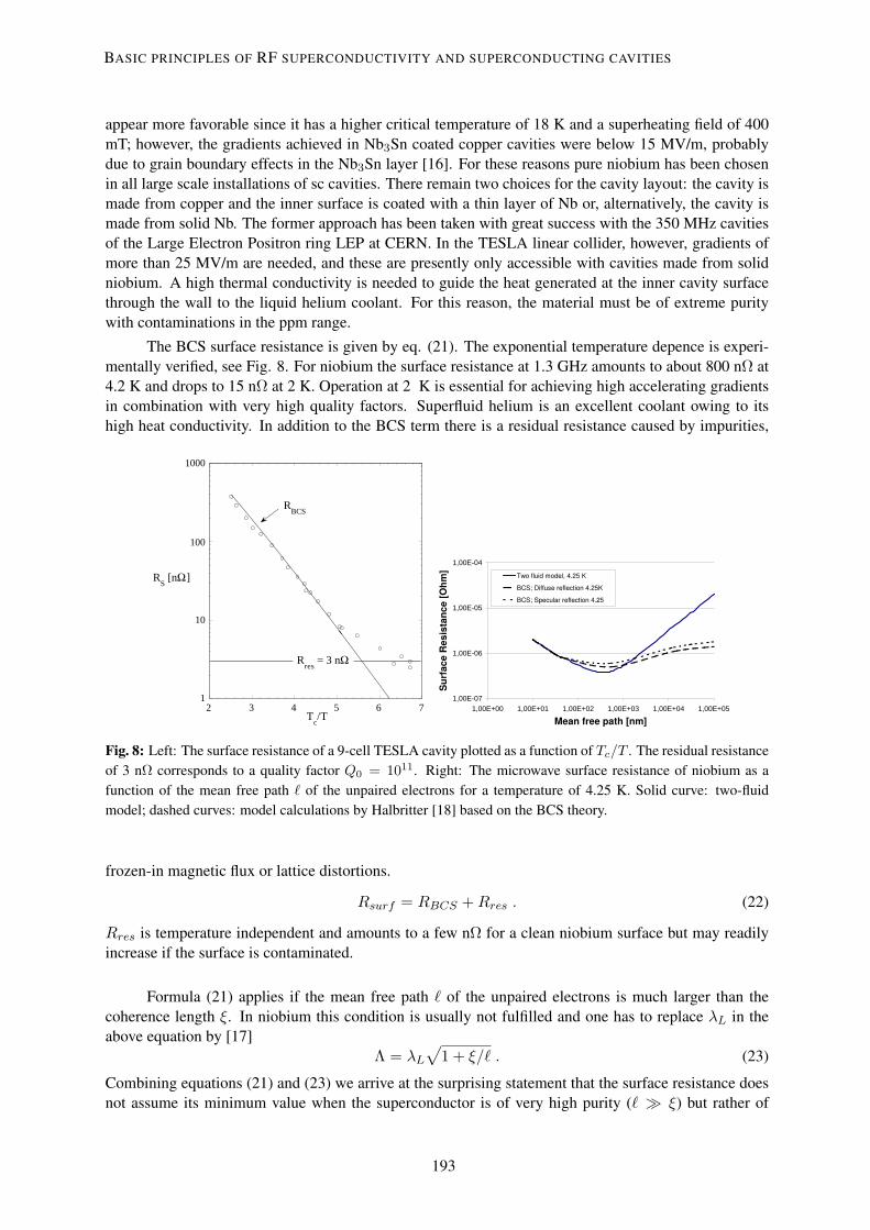
The BCS surface resistance is given by eq. (21). The exponential temperature depence is experi-mentally verified, see Fig. 8. For niobium the surface resistance at 1.3 GHz amounts to about 800 nΩ at4.2 K and drops to 15 nΩ at 2 K. Operation at 2 K is essential for achieving high accelerating gradientsin combination with very high quality factors. Superfluid helium is an excellent coolant owing to itshigh heat conductivity. In addition to the BCS term there is a residual resistance caused by impurities,

2 3 4 5 6 7

RS [nΩ]

Tc/T

Rres

= 3 nΩ

1000

100

10

1

RBCS

1,00E-07

1,00E-06

1,00E-05

1,00E-04

1,00E+00 1,00E+01 1,00E+02 1,00E+03 1,00E+04 1,00E+05

Fig. 8: Left: The surface resistance of a 9-cell TESLA cavity plotted as a function of Tc/T . The residual resistanceof 3 nΩ corresponds to a quality factor Q0 = 1011. Right: The microwave surface resistance of niobium as afunction of the mean free path ` of the unpaired electrons for a temperature of 4.25 K. Solid curve: two-fluidmodel; dashed curves: model calculations by Halbritter [18] based on the BCS theory.

frozen-in magnetic flux or lattice distortions.

Rsurf = RBCS + Rres . (22)

Rres is temperature independent and amounts to a few nΩ for a clean niobium surface but may readilyincrease if the surface is contaminated.

Formula (21) applies if the mean free path ` of the unpaired electrons is much larger than thecoherence length ξ. In niobium this condition is usually not fulfilled and one has to replace λL in theabove equation by [17]

Λ = λL

√1 + ξ/` . (23)

Combining equations (21) and (23) we arrive at the surprising statement that the surface resistance doesnot assume its minimum value when the superconductor is of very high purity (` ξ) but rather of

11


193

moderate purity with a mean free path ` ≈ ξ, see Fig. 8. The measured BCS resistance in the sputter-coated LEP cavities is in fact a factor of two lower than in bulk niobium cavities [19]. The sputteredniobium layer has a low RRR (see sect. 3.6) and an electron mean free path ` ≈ ξ.

3.2 Pill box cavityThe simplest model of an accelerating cavity is a hollow cylinder which is often called pill box. Whenthe beam pipes are neglected the field pattern inside the resonator and all relevant cavity parameters canbe calculated analytically.

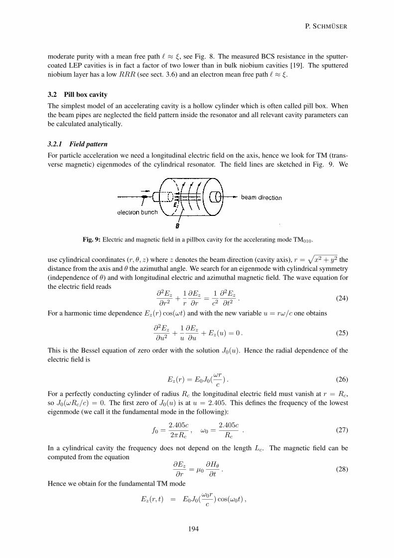
3.2.1 Field patternFor particle acceleration we need a longitudinal electric field on the axis, hence we look for TM (trans-verse magnetic) eigenmodes of the cylindrical resonator. The field lines are sketched in Fig. 9. We

Fig. 9: Electric and magnetic field in a pillbox cavity for the accelerating mode TM010.

use cylindrical coordinates (r, θ, z) where z denotes the beam direction (cavity axis), r =√

x2 + y2 thedistance from the axis and θ the azimuthal angle. We search for an eigenmode with cylindrical symmetry(independence of θ) and with longitudinal electric and azimuthal magnetic field. The wave equation forthe electric field reads

∂2Ez

∂r2+

1r

∂Ez

∂r=

1c2

∂2Ez

∂t2. (24)

For a harmonic time dependence Ez(r) cos(ωt) and with the new variable u = rω/c one obtains

∂2Ez

∂u2+

1u

∂Ez

∂u+ Ez(u) = 0 . (25)

This is the Bessel equation of zero order with the solution J0(u). Hence the radial dependence of theelectric field is

Ez(r) = E0J0(ωr

c) . (26)

For a perfectly conducting cylinder of radius Rc the longitudinal electric field must vanish at r = Rc,so J0(ωRc/c) = 0. The first zero of J0(u) is at u = 2.405. This defines the frequency of the lowesteigenmode (we call it the fundamental mode in the following):

f0 =2.405c

2πRc, ω0 =

2.405c

Rc. (27)

In a cylindrical cavity the frequency does not depend on the length Lc. The magnetic field can becomputed from the equation

∂Ez

∂r= µ0

∂Hθ

∂t. (28)

Hence we obtain for the fundamental TM mode

Ez(r, t) = E0J0(ω0r

c) cos(ω0t) ,

12

P. SCHMUSER

194

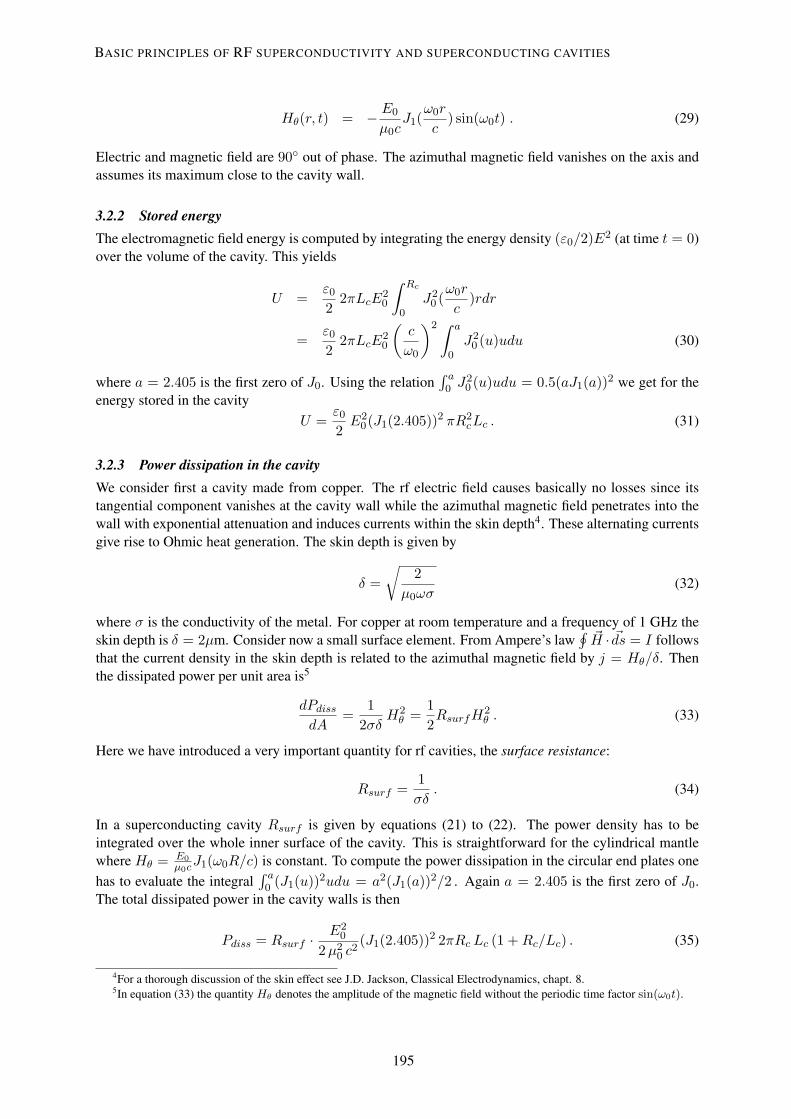
Hθ(r, t) = − E0

µ0cJ1(

ω0r

c) sin(ω0t) . (29)

Electric and magnetic field are 90 out of phase. The azimuthal magnetic field vanishes on the axis andassumes its maximum close to the cavity wall.

3.2.2 Stored energyThe electromagnetic field energy is computed by integrating the energy density (ε0/2)E2 (at time t = 0)over the volume of the cavity. This yields

U =ε0

22πLcE

20

∫ Rc

0J2

0 (ω0r

c)rdr

=ε0

22πLcE

20

(c

ω0

)2 ∫ a

0J2

0 (u)udu (30)

where a = 2.405 is the first zero of J0. Using the relation∫ a0 J2

0 (u)udu = 0.5(aJ1(a))2 we get for theenergy stored in the cavity

U =ε0

2E2

0(J1(2.405))2 πR2cLc . (31)

3.2.3 Power dissipation in the cavityWe consider first a cavity made from copper. The rf electric field causes basically no losses since itstangential component vanishes at the cavity wall while the azimuthal magnetic field penetrates into thewall with exponential attenuation and induces currents within the skin depth4. These alternating currentsgive rise to Ohmic heat generation. The skin depth is given by

δ =√

2µ0ωσ

(32)

where σ is the conductivity of the metal. For copper at room temperature and a frequency of 1 GHz theskin depth is δ = 2µm. Consider now a small surface element. From Ampere’s law

∮~H · ~ds = I follows

that the current density in the skin depth is related to the azimuthal magnetic field by j = Hθ/δ. Thenthe dissipated power per unit area is5

dPdiss

dA=

12σδ

H2θ =

12RsurfH2

θ . (33)

Here we have introduced a very important quantity for rf cavities, the surface resistance:

Rsurf =1σδ

. (34)

In a superconducting cavity Rsurf is given by equations (21) to (22). The power density has to beintegrated over the whole inner surface of the cavity. This is straightforward for the cylindrical mantlewhere Hθ = E0

µ0cJ1(ω0R/c) is constant. To compute the power dissipation in the circular end plates onehas to evaluate the integral

∫ a0 (J1(u))2udu = a2(J1(a))2/2 . Again a = 2.405 is the first zero of J0.

The total dissipated power in the cavity walls is then

Pdiss = Rsurf ·E2

0

2 µ20 c2

(J1(2.405))2 2πRc Lc (1 + Rc/Lc) . (35)

4For a thorough discussion of the skin effect see J.D. Jackson, Classical Electrodynamics, chapt. 8.5In equation (33) the quantity Hθ denotes the amplitude of the magnetic field without the periodic time factor sin(ω0t).

13


195

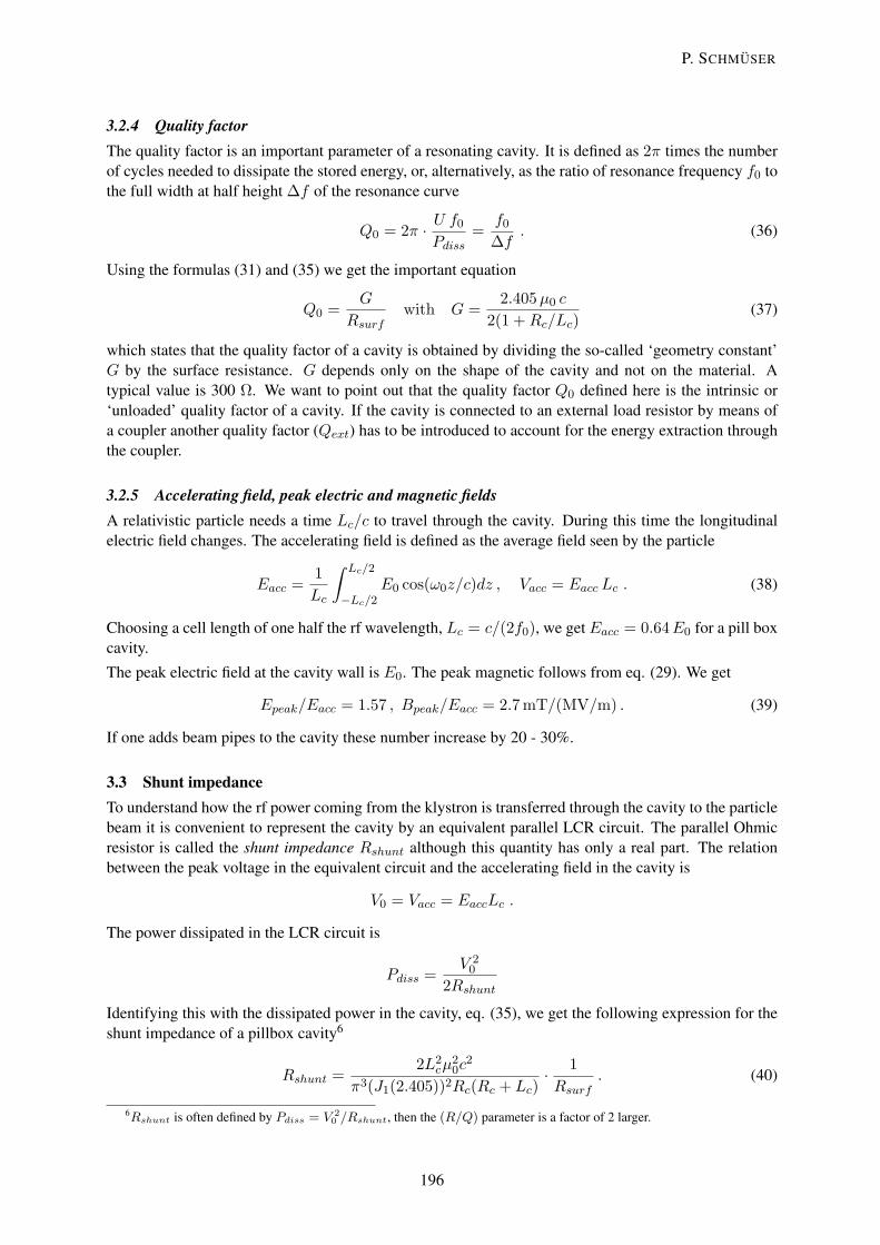
3.2.4 Quality factorThe quality factor is an important parameter of a resonating cavity. It is defined as 2π times the numberof cycles needed to dissipate the stored energy, or, alternatively, as the ratio of resonance frequency f0 tothe full width at half height ∆f of the resonance curve

Q0 = 2π · U f0

Pdiss=

f0

∆f. (36)

Using the formulas (31) and (35) we get the important equation

Q0 =G

Rsurfwith G =

2.405 µ0 c

2(1 + Rc/Lc)(37)

which states that the quality factor of a cavity is obtained by dividing the so-called ‘geometry constant’G by the surface resistance. G depends only on the shape of the cavity and not on the material. Atypical value is 300 Ω. We want to point out that the quality factor Q0 defined here is the intrinsic or‘unloaded’ quality factor of a cavity. If the cavity is connected to an external load resistor by means ofa coupler another quality factor (Qext) has to be introduced to account for the energy extraction throughthe coupler.

3.2.5 Accelerating field, peak electric and magnetic fieldsA relativistic particle needs a time Lc/c to travel through the cavity. During this time the longitudinalelectric field changes. The accelerating field is defined as the average field seen by the particle

Eacc =1Lc

∫ Lc/2

−Lc/2E0 cos(ω0z/c)dz , Vacc = Eacc Lc . (38)

Choosing a cell length of one half the rf wavelength, Lc = c/(2f0), we get Eacc = 0.64 E0 for a pill boxcavity.

The peak electric field at the cavity wall is E0. The peak magnetic follows from eq. (29). We get

Epeak/Eacc = 1.57 , Bpeak/Eacc = 2.7 mT/(MV/m) . (39)

If one adds beam pipes to the cavity these number increase by 20 - 30%.

3.3 Shunt impedanceTo understand how the rf power coming from the klystron is transferred through the cavity to the particlebeam it is convenient to represent the cavity by an equivalent parallel LCR circuit. The parallel Ohmicresistor is called the shunt impedance Rshunt although this quantity has only a real part. The relationbetween the peak voltage in the equivalent circuit and the accelerating field in the cavity is

V0 = Vacc = EaccLc .

The power dissipated in the LCR circuit is

Pdiss =V 2

0

2Rshunt

Identifying this with the dissipated power in the cavity, eq. (35), we get the following expression for theshunt impedance of a pillbox cavity6

Rshunt =2L2

cµ20c

2

π3(J1(2.405))2Rc(Rc + Lc)· 1Rsurf

. (40)

6Rshunt is often defined by Pdiss = V 20 /Rshunt, then the (R/Q) parameter is a factor of 2 larger.

14

P. SCHMUSER

196

The surface resistance of a superconducting cavity is extremely small, about 15 nΩ at 2 K; consequently,the shunt impedance is extremely large, in the order of 5 · 1012 Ω. Note that “on resonance” (ω = ω0 =1/√

LC) the parallel LCR circuit behaves like a purely Ohmic resistor whose value is equal to the shuntimpedance.

The ratio of shunt impedance to quality factor is an important cavity parameter

(R/Q) ≡ Rshunt

Q0=

4Lcµ0c

π3(J1(2.405))22.405Rc(41)

The (R/Q) parameter is independent of the material, it depends only on the shape of the cavity. A typicalvalue for a 1-cell cavity is (R/Q) = 100 Ω.

3.4 Shape of practical cavitiesThe first sc cavities were built in the late 1960’s with the conventional pill-box shape. They showedunexpected performance limitations: at field levels of a few MV/m a phenomen called multiple impacting(or multipacting for short) was observed. The effect is as follows: stray electrons which are releasedfrom the wall (for instance by cosmic rays) gain energy in one half-period of the electromagnetic fieldand return to their origin in the next half period were they impinge with a few 100 eV onto the walland release secondary electrons which repeat the same procedure. This way an avalanche of electronsis created which absorbs energy from the rf field, heats the superconductor and eventually leads to abreakdown of superconductivity. It was found out many years later that this problem is avoided in cavitieshaving the shape of a rotational ellipsoid. When electrons are emitted near the iris of an elliptical cavityand accelerated by the rf field, they return to a point away from their origin in the next half period, andthe same applies for the possible next generations of electrons. Thereby the daughter electrons movemore and more into the equator region where the rf electric field is small and the multiplication processdies out. For a thorough discussion I refer to [10].

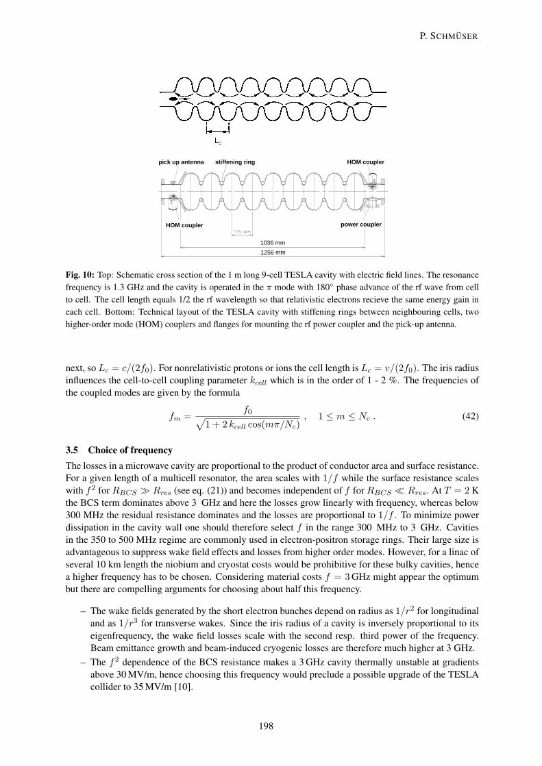
In electron-positron storage rings quite often single-cell cavities are used. These are particularlywell suited for the large beam currents of up to 1 A in the high luminosity ’B meson factories’. At largerenergies like in LEP (104 GeV per beam) multicell cavities are more efficient to compensate for the hugesynchrotron radiation losses (3 GeV per revolution in LEP). In a linear collider almost the full length ofthe machine must be filled with accelerating structures and then long multicell cavities are mandatory.There are, however, several effects which limit the number of cells Nc per resonator. With increasingNc it becomes more and more difficult to tune the resonator for equal field amplitude in every cell.Secondly, in a very long multicell cavity ’trapped modes’ may be excited by the short particle bunches.These are coupled oscillations at high frequency which are confined to the inner cells and have such alow amplitude in the beam pipe sections that they cannot be extracted by a higher-order mode coupler.Trapped modes have a negative influence on the following bunches and must be avoided. The numberNc = 9 chosen for TESLA appears a reasonable upper limit. The TESLA cavity [22] is shown in Fig.10.

Superconducting cavities are always operated in standing-wave mode7. The fundamental TM010

mode is chosen with a longitudinal electric field on the axis. In a cavity with Nc cells the fundamentalmode splits into Nc coupled modes. The π mode with 180 phase difference between adjacent cellstransfers the highest possible energy to the particles. The cell length Lc is determined by the conditionthat the electric field has to be inverted in the time a relativistic particle needs to travel from one cell to the

7In normal-conducting linacs like SLAC the travelling wave mode may be chosen. Basically the electrons ’ride’ on thecrests of the rf wave which propagates with the speed of light. In a superconducting linac a travelling wave is not attenuated bywall losses, and in order to preserve the basic advantage of superconductivity - almost no rf power is wasted - one would have toextract the rf wave after some length and feed it back through a superconducting wave guide to the input coupler. The requiredprecision in rf phase would be extremely demanding and would make such a system far more complicated than a standing-wavelinac.

15


197

stiffening ring HOM couplerpick up antenna

HOM coupler power coupler

1036 mm

1256 mm

Fig. 10: Top: Schematic cross section of the 1 m long 9-cell TESLA cavity with electric field lines. The resonancefrequency is 1.3 GHz and the cavity is operated in the π mode with 180 phase advance of the rf wave from cellto cell. The cell length equals 1/2 the rf wavelength so that relativistic electrons recieve the same energy gain ineach cell. Bottom: Technical layout of the TESLA cavity with stiffening rings between neighbouring cells, twohigher-order mode (HOM) couplers and flanges for mounting the rf power coupler and the pick-up antenna.

next, so Lc = c/(2f0). For nonrelativistic protons or ions the cell length is Lc = v/(2f0). The iris radiusinfluences the cell-to-cell coupling parameter kcell which is in the order of 1 - 2 %. The frequencies ofthe coupled modes are given by the formula

fm =f0√

1 + 2 kcell cos(mπ/Nc), 1 ≤ m ≤ Nc . (42)

3.5 Choice of frequencyThe losses in a microwave cavity are proportional to the product of conductor area and surface resistance.For a given length of a multicell resonator, the area scales with 1/f while the surface resistance scaleswith f2 for RBCS Rres (see eq. (21)) and becomes independent of f for RBCS Rres. At T = 2 Kthe BCS term dominates above 3 GHz and here the losses grow linearly with frequency, whereas below300 MHz the residual resistance dominates and the losses are proportional to 1/f . To minimize powerdissipation in the cavity wall one should therefore select f in the range 300 MHz to 3 GHz. Cavitiesin the 350 to 500 MHz regime are commonly used in electron-positron storage rings. Their large size isadvantageous to suppress wake field effects and losses from higher order modes. However, for a linac ofseveral 10 km length the niobium and cryostat costs would be prohibitive for these bulky cavities, hencea higher frequency has to be chosen. Considering material costs f = 3 GHz might appear the optimumbut there are compelling arguments for choosing about half this frequency.

– The wake fields generated by the short electron bunches depend on radius as 1/r2 for longitudinaland as 1/r3 for transverse wakes. Since the iris radius of a cavity is inversely proportional to itseigenfrequency, the wake field losses scale with the second resp. third power of the frequency.Beam emittance growth and beam-induced cryogenic losses are therefore much higher at 3 GHz.

– The f2 dependence of the BCS resistance makes a 3 GHz cavity thermally unstable at gradientsabove 30 MV/m, hence choosing this frequency would preclude a possible upgrade of the TESLAcollider to 35 MV/m [10].

16

P. SCHMUSER

198

3.6 Heat conduction in niobium and heat transfer to the liquid helium

1 101

10

100

1000

8642 20

RRR = 500 RRR = 270

λ[W

/mK

]

T [K]

Fig. 11: Measured heat conductivity in niobium samples with RRR = 270 and RRR = 500 as a function oftemperature [20].

The heat produced at the inner cavity surface has to be guided through the cavity wall to thesuperfluid helium bath. At 2 - 4 K, impurities have a strong impact on the thermal conductivity of metals.Niobium of very high purity is needed (contamination in the ppm range). The heat conductivity dropsby about an order of magnitude when lowering the temperature from 4 to 2 K, as shown in Fig. 11. Theresidual resistivity ratio RRR = R(300K)/R(10K) is a good measure for the purity of the material:large RRR means high electrical and thermal conductivity at low temperature.

The beneficial effect of a high thermal conductivity on the cavity performance is demonstrated inFig. 12. Here the quality factor Q0 is plotted as a function of the accelerating field Eacc for a nine-cellTESLA cavity before and after a 1400C heat treatment. The RRR of the niobium increases during thistreatment from 380 to 760, and obviously the cavity can be excited to higher fields afterwards. What onecan also observe in this figure is a drop of the quality factor towards high fields. The main reason is in thiscase the onset of electron field emission (see below). These electrons are accelerated in the rf field andimpinge on the cavity walls where they deposit energy and may even generate X rays by bremsstrahlung.

109

1010

1011

0 5 10 15 20 25 30

HT 800 °C, RRR 380HT 1400 °C, RRR 760

Q0

Eacc

[MV/m]

quench

no quenchlimited by amplifier

x-ray starts

Fig. 12: The excitation curve Q0 = Q0(Eacc) of a nine-cell TESLA cavity before and after the heat treatment at1400C.

17


199

1,0E+08

1,0E+09

1,0E+10

1,0E+11

0 10 20 30 40Eacc [MV/m]

Q0

1,0E+09

1,0E+10

1,0E+11

0 10 20 30 40

Eacc [MV/m]

Q0

Fig. 13: Excitation curves of electropolished cavities at a helium temperature of 2 K. Left: 1-cell cavities, right:9-cell cavity.

Low frequency cavities (350-500 MHz) have a small BCS surface resistance at 4.2 K and areeffectively cooled by normal liquid helium. The heat flux should not exceed a few kW/m2 to obtainnucleate boiling with a close contact between liquid and metal. At higher heat fluxes one enters the filmboiling regime where a vapour film covers the surface. Here the cavity may easily warm up beyond Tc atareas of excessive heating. The f2 dependence of the BCS resistance implies that for cavities of higherfrequency superfluid helium at 1.8 - 2 K is more appropriate. At the metal-helium interface a temperaturejump is observed which is attributed to phonon mismatch. The so-called Kapitza resistance amounts toabout 1.5 · 10−4 m2K/W [21] for a clean niobium surface in contact with superfluid helium.

3.7 Maximum accelerating fieldSuperconductivity breaks down when the microwave magnetic field at the cavity surface exceeds a crit-ical value. The situation is clearcut for a type I superconductor such as lead where the superconductingstate prevails up to Bc = 80 mT. For the type II conductor niobium it is not so obvious which of thecritical fields should be used. The values at 2 K are approximately

– Bc1 = 160 mT– Bc = 190 mT– Bc2 = 300 mT

A very safe value would be Bc1 because then no magnetic flux enters the bulk niobium. The correspond-ing gradient of 38 MV/m in TESLA-type cavities has been definitely exceeded in single-cell cavities,more than 40 MV/m have been repeatedly reached. There is some evidence that the maximum tolerablerf magnetic field is close to the thermodynamic critical field of 190 mT but the issue is not finally settledyet.

The most promising road towards the ultimate gradient is a cavity surface preparation by elec-trolytic polishing. In figure 13 we show the performance of several electropolished cavities. Theseresults prove that a centre-of-mass energy of 800 GeV can indeed be reached in the TESLA electron-positron collider.

3.8 Thermal instability and field emissionThe fundamental advantage of superconducting cavities is their extremely low surface resistance of about10 nΩ at 2 K, leading to rf losses which are 5 to 6 orders of magnitude lower than in copper cavities. Thedrawback is that even tiny surface contaminations are potentially harmful as they decrease the quality

18

P. SCHMUSER

200

factor and may even lead to a thermal breakdown (quench) of the superconductor due to local overheat-ing.

Temperature mapping at the outer cavity wall usually reveals that the heating is not uniform overthe whole surface but that certain spots exhibit larger temperature rises, often beyond the critical tem-perature of the superconductor. Hence the cavity becomes partially normal-conducting, associated withstrongly enhanced power dissipation. Because of the exponential increase of surface resistance withtemperature this may result in a run-away effect and eventually a quench of the entire cavity. Analyticalmodels and numerical codes are available to describe this effect. The tolerable defect size depends onthe purity of the material. As a typical number, the diameter of a normal-conducting spot must be lessthan 50 µm to avoid a thermal instability at 25 MV/m.

Field emission of electrons from sharp tips has been a notorious limitation of high-gradient sccavities. The typical indication is that the quality factor drops exponentially above a certain thresholdfield, and X rays are observed. The field emission current density is given by the Fowler-Nordheimequation [23], adapted for rf fields:

jFE ∝E2.5

loc

Φexp(−CΦ3/2/Eloc) . (43)

Here Φ is the work function of the metal, C a constant and Eloc the local electric field. At sharp tips onthe surface the local field may be several 100 times larger than the accelerating field. Perfect cleaning byrinsing with high-pressure ultrapure water is the most effective remedy against field emission. Using theclean room techniques developed in semiconductor industry it has been possible to raise the thresholdfor field emission in multicell cavities from about 10 MV/m to more than 20 MV/m in the past few years.Thermal instabilities and field emission are discussed at much greater detail in [10].

References[1] P. Schmuser, Superconductivity in High Energy Particle Accelerators, Prog. Part. Nucl. Phys.

49 (2002) issue 1. Available from the internet: http://wwww.desy.de/~pschmues, filesupercon-acc.pdf

[2] Review of Particle Properties, Europ. Phys. Journ. C15 (2000)[3] C. Adolphsen et al., SLAC Report 474 (1996)[4] JLC Design Study, KEK Report 97-1 (1997)[5] G. Guignard et al., CERN Report 2000-008 (2000)[6] B.H. Wiik, Part. Acc. 62 (1998) 563[7] TESLA, Technical Design Report, The Accelerator, Eds. R. Brinkmann, K. Flottmann, J. Rossbach,

P. Schmuser, N. Walker, H. Weise, DESY report 2001-23 (2001)[8] G.A. Krafft, Status of the Continuous Electron Beam Accelerator Facility, Proc 1994 Linear Accel.

Conf., 9 (1994)[9] International Linear Collider Technical Review Committee Report II (2002), ed. G.A. Loew, to be

published[10] H. Padamsee, J. Knobloch and T. Hays, RF Superconductivity for Accelerators, John Wiley, New

York 1998.[11] H. Piel in: Proc. of the 1988 CERN Accelerator School Superconductivity in Particle Accelerators,

CERN report 89-04 (1989)[12] D.C. Larbalestier and P.J. Lee, Proc. PAC99, New York (1999) 177[13] W. Buckel, Supraleitung, VCH Verlagsgesellschaft, Weinheim 1990[14] D.R. Tilley and J. Tilley, Superfluidity and Superconductivity, Institute of Physics Publishing Ltd,

Bristol 1990

19


201

[15] E.W. Collings et al., Adv. Cryog. Eng. 36 (1990) 169[16] G. Muller, Proc. 3rd Workshop on RF Superconductivity, ed. K.W. Shepard, Argonne, USA (1988),

p. 331[17] B. Bonin, CERN Accelerator School Superconductivity in Particle Accelerators, CERN 96-03, ed.

S. Turner, Hamburg (1995)[18] J. Halbritter, Z. Physik 238 (1970) 466[19] C. Benvenuti et al., Proc. PAC91, San Francisco (1991), p. 1023.[20] T. Schilcher, TESLA-Report, TESLA 95-12, DESY (1995)[21] A. Boucheffa et al., Proc. 7th Workshop on RF Superconductivity, ed. B. Bonin, Gif-sur-Yvette,

France (1995), p. 659[22] B. Aune et al., Phys. Rev. Spec. Top. Acc. Beams PRSTAB 3 (2000) 092001[23] R.H. Fowler and L. Nordheim, Proc. of the Roy. Soc. A 119, 173 and Math. Phys. Sci. 119 (1928)

173.

20

P. SCHMUSER

202

Documents

Basic principles of RF superconductivity and ... · PDF file1.1 Advantages and limitations of superconductor technology in accelerators The vanishing electrical resistance ... needed