Embed Size (px)
Citation preview

Basic Principles of Probability and Statistics
Lecture notes for PET 472
Spring 2010
Prepared by: Thomas W. Engler, Ph.D., P.E

Definitions
• Risk Analysis
– Assessing probabilities of occurrence for each possible outcome
Risk AnalysisProbabilities and prob. distributionsRepresenting judgments about chanceevents
ModelingGeologic, reservoir, drillingOperations, Economics
Decision criteriaEV, profit, IRR…
Present to management for decision

Definitions
• Sample Space– Complete set of outcomes
(52 cards)
• Outcome– Subset of the sample space
(drawing a “5” of any suit)
• Probability– Likelihood of drawing a “5”
P(A) = 4/52
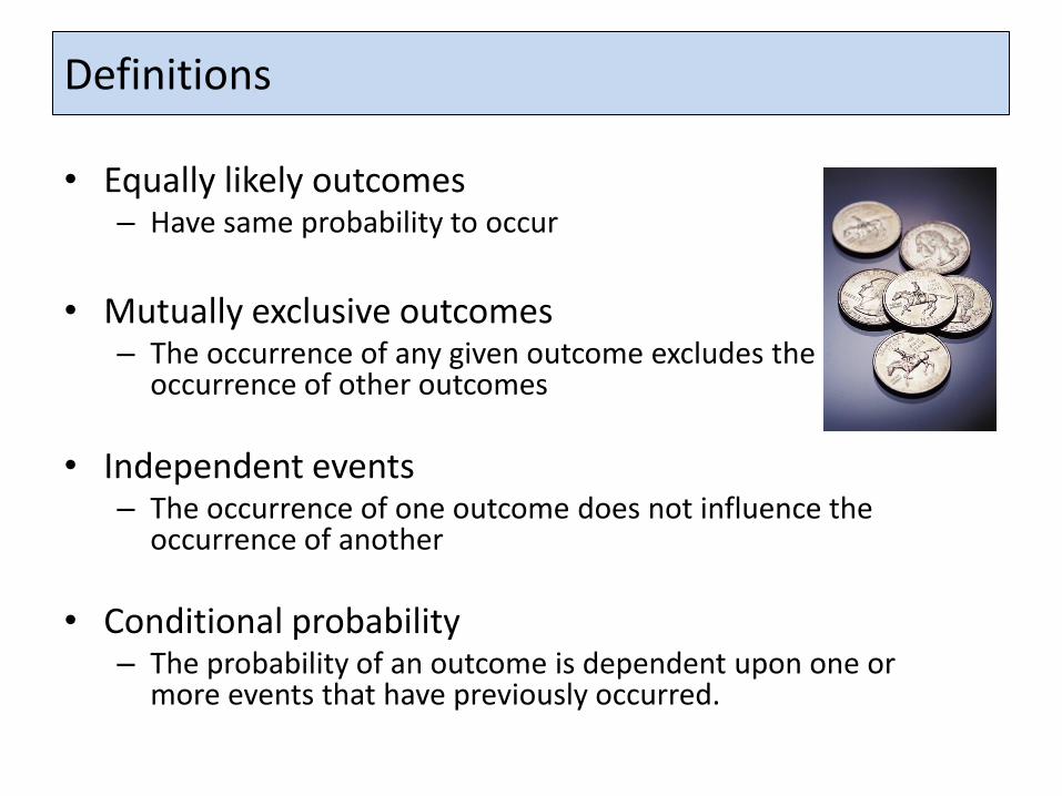
Definitions
• Equally likely outcomes– Have same probability to occur
• Mutually exclusive outcomes– The occurrence of any given outcome excludes the
occurrence of other outcomes
• Independent events– The occurrence of one outcome does not influence the
occurrence of another
• Conditional probability– The probability of an outcome is dependent upon one or
more events that have previously occurred.

Rules of Operation
Symbol Definition Expression
P(A) Probability of outcome A occurring
P(A+B) Probability of outcome A and/or B occurring
P(A+B)=P(A)+P(B)-P(AB)
P(AB) Probability of A and B occurring P(AB) = P(A) P(B|A)
P(A|B) Probability of A given B has occurred.

Rules of Operation
P(A+B)=P(A)+P(B)-P(AB)
Addition Theorem
Exampleoutcome A – drawing 4, 5, 6 of any suit
outcome B – J or Q of any suit
52
12)A(P
52
8)B(P
0)AB(P52
20)BA(P
A
B
Venn Diagram
MutuallyExclusiveevents

Rules of Operation
P(A+B)=P(A)+P(B)-P(AB)
Addition Theorem
Exampleoutcome A – drawing 4, 5, 6 of any suit
outcome B – drawing a diamond
52
12)A(P
52
13)B(P
52
3)AB(P52
22)BA(P
AB
Venn Diagram

Rules of Operation
P(AB)=P(A)P(A|B)
Multiplication Theorem
Exampleoutcome A – drawing any jack
outcome B – drawing a four of heartson the second draw
52
4)A(P
51
1)A|B(P
663
1
51
1
52
4)AB(P
Sampling without replacement- observed outcome is not returned- series of dependent events
conditional
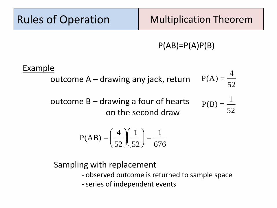
Rules of Operation
P(AB)=P(A)P(B)
Multiplication Theorem
Exampleoutcome A – drawing any jack, return
outcome B – drawing a four of heartson the second draw
52
4)A(P
52
1)B(P
676
1
52
1
52
4)AB(P
Sampling with replacement- observed outcome is returned to sample space- series of independent events
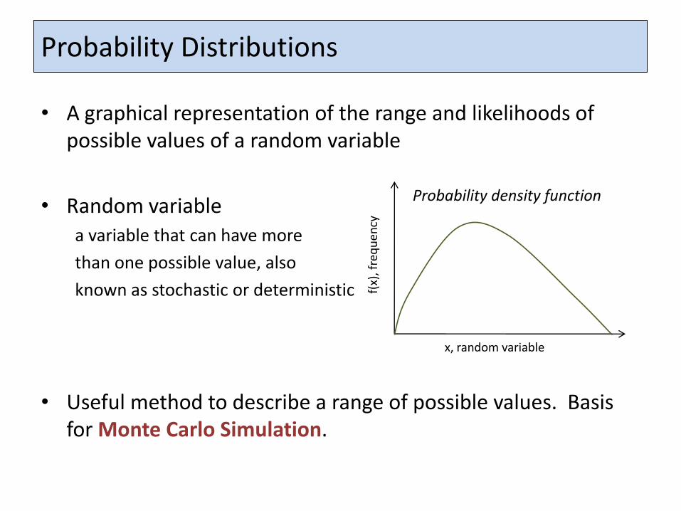
Probability Distributions
• A graphical representation of the range and likelihoods of possible values of a random variable
• Random variable a variable that can have more
than one possible value, also
known as stochastic or deterministic
• Useful method to describe a range of possible values. Basis for Monte Carlo Simulation.
x, random variable
f(x)
, fre
qu
ency
Probability density function

Probability Distributions
Histogram representation Of statistical data
Data
Well No Net pay, ft
1 111
2 81
3 142
4 59
5 109
6 96
7 124
8 139
9 89
10 129
11 104
12 186
13 65
14 95
15 54
16 72
17 167
18 135
19 84
20 154
Divide into intervals Or bins
Range frequency Percent
50 - 80 4 20%
81 - 110 7 35%
111 - 140 5 25%
141 - 170 3 15%
171 - 200 1 5%
20 100%
0%
5%
10%
15%
20%
25%
30%
35%
40%
0
1
2
3
4
5
6
7
8
50 - 80 81 - 110 111 - 140 141 - 170 171 - 200
Pe
rce
nt
fre
qu
en
cy
Net Pay, feet
Frequency distributions

Probability Distributions
Benefits1. Can easily read probabilities2. Necessary for Monte Carlo
Simulation
minimum
Cumulative frequency distributions
Cumulative
Range Percent ≤
50 0%
80 20%
110 55%
140 80%
170 95%
200 100%
0%
20%
40%
60%
80%
100%
0 50 100 150 200
Cu
mu
lati
ve p
erc
en
t ≤
Net Pay, feet
Range frequency Percent
50 - 80 4 20%
81 - 110 7 35%
111 - 140 5 25%
141 - 170 3 15%
171 - 200 1 5%
20 100%
maximum
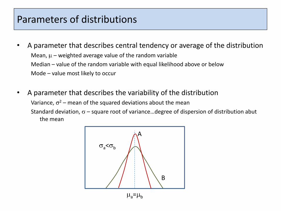
Parameters of distributions
• A parameter that describes central tendency or average of the distributionMean, – weighted average value of the random variable
Median – value of the random variable with equal likelihood above or below
Mode – value most likely to occur
• A parameter that describes the variability of the distributionVariance, 2 – mean of the squared deviations about the mean
Standard deviation, – square root of variance…degree of dispersion of distribution abut the mean
A
B
a= b
a< b

Parameters of distributions Computing mean and standard deviation
1. Arithmetic average of discrete sample data setDepth k,md , %
4807.5 2.5 17.0
4808.5 59 20.7
4809.5 221 19.1
4810.5 211 20.4
4811.5 275 23.3
4812.5 384 24.0
4813.5 108 23.3
4814.5 147 16.1
4815.5 290 17.2
4816.5 170 15.3
4817.5 278 15.9
4818.5 238 18.6
4819.5 167 16.2
4820.5 304 20.0
4821.5 98 16.9
4822.5 191 18.1
4823.5 266 20.3
4824.5 40 15.3
4825.5 260 15.1
4826.5 179 14.0
4827.5 312 15.6
4828.5 272 15.5
4829.5 395 19.4
4830.5 405 17.5
4831.5 275 16.4
4832.5 852 17.2
4833.5 610 15.5
4834.5 406 20.2
4835.5 535 18.3
4836.5 663 19.6
4837.5 597 17.7
4838.5 434 20.0
4839.5 339 16.8
4840.5 216 13.3
4841.5 332 18.0
4842.5 295 16.1
4843.5 882 15.1
4844.5 600 18.0
4845.5 407 15.7
4847.5 479 17.8
4847.5 139 20.5
4847.5 135 8.4
17.6
2.87
17.6
2.87
Core porosity and permeability
N
N
1i
2)
ix(
N – number of equally-probable valuesN
N
1ii
x
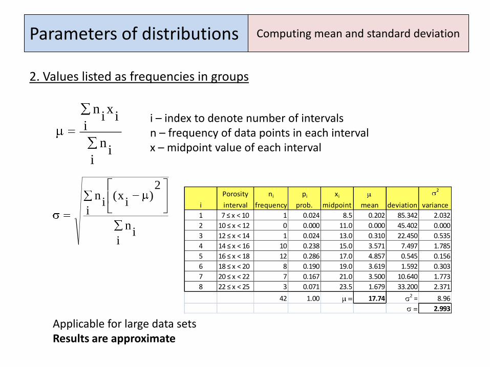
Parameters of distributions Computing mean and standard deviation
2. Values listed as frequencies in groups
ii
n
ii
xi
ni – index to denote number of intervalsn – frequency of data points in each intervalx – midpoint value of each interval
ii
n
i
2)
ix(
in Porosity ni pi xi
2
i interval frequency prob. midpoint mean deviation variance
1 7 ≤ x < 10 1 0.024 8.5 0.202 85.342 2.032
2 10 ≤ x < 12 0 0.000 11.0 0.000 45.402 0.000
3 12 ≤ x < 14 1 0.024 13.0 0.310 22.450 0.535
4 14 ≤ x < 16 10 0.238 15.0 3.571 7.497 1.785
5 16 ≤ x < 18 12 0.286 17.0 4.857 0.545 0.156
6 18 ≤ x < 20 8 0.190 19.0 3.619 1.592 0.303
7 20 ≤ x < 22 7 0.167 21.0 3.500 10.640 1.773
8 22 ≤ x < 25 3 0.071 23.5 1.679 33.200 2.371
42 1.00 17.74 2 = 8.96
2.993
Applicable for large data setsResults are approximate

Parameters of distributions Computing mean and standard deviation
3. Discrete probability distributions
x midpoint
drilling costs probability of range EV xi*pi (xi- )2 p(xi)(xi- )
$M $M $M $M ($M)2 ($M)2
100.0 0
105.2 0.007 102.6 0.7 0.7 1641.3 10.7
111.5 0.040 108.4 4.3 4.5 1208.5 48.3
130.6 0.229 121.1 27.7 29.9 486.8 111.5
136.3 0.093 133.5 12.4 12.7 93.4 8.7
148.2 0.225 142.3 32.0 33.3 0.7 0.2
165.2 0.278 156.7 43.6 45.9 184.6 51.3
168.7 0.035 167.0 5.8 5.9 568.2 19.9
178.5 0.066 173.6 11.5 11.8 929.5 61.3
183.7 0.021 181.1 3.8 3.9 1443.0 30.3
190.0 0.007 186.9 1.3 1.3 1912.9 13.4
143.1 149.9 355.6
15.8 18.9
ii
xi
p
i
2)
ix(
ip
pi is the probability of occurrence of the xith value of the random variable
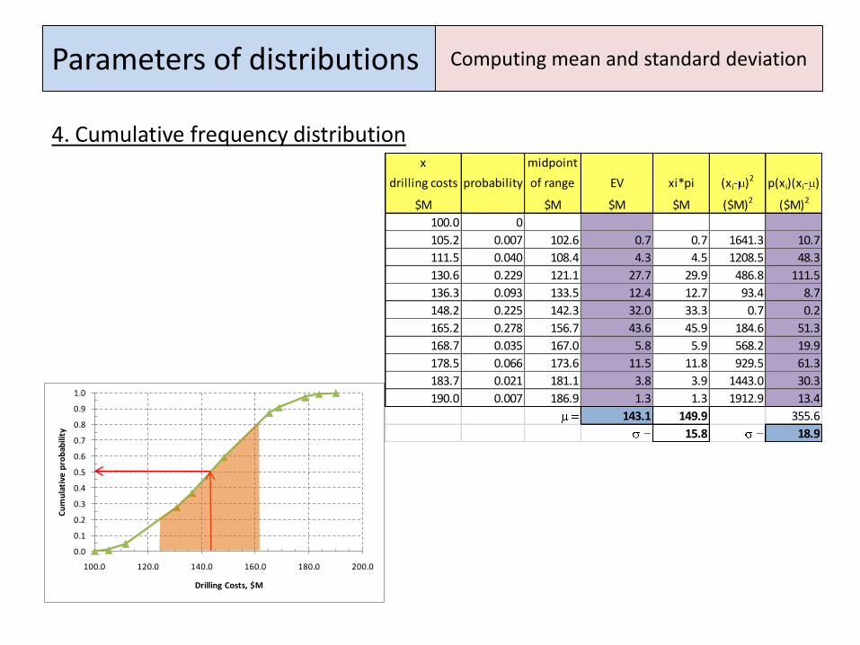
Parameters of distributions Computing mean and standard deviation
4. Cumulative frequency distributionx midpoint
drilling costs probability of range EV xi*pi (xi- )2 p(xi)(xi- )
$M $M $M $M ($M)2 ($M)2
100.0 0
105.2 0.007 102.6 0.7 0.7 1641.3 10.7
111.5 0.040 108.4 4.3 4.5 1208.5 48.3
130.6 0.229 121.1 27.7 29.9 486.8 111.5
136.3 0.093 133.5 12.4 12.7 93.4 8.7
148.2 0.225 142.3 32.0 33.3 0.7 0.2
165.2 0.278 156.7 43.6 45.9 184.6 51.3
168.7 0.035 167.0 5.8 5.9 568.2 19.9
178.5 0.066 173.6 11.5 11.8 929.5 61.3
183.7 0.021 181.1 3.8 3.9 1443.0 30.3
190.0 0.007 186.9 1.3 1.3 1912.9 13.4
143.1 149.9 355.6
15.8 18.9
0.0
0.1
0.2
0.3
0.4
0.5
0.6
0.7
0.8
0.9
1.0
100.0 120.0 140.0 160.0 180.0 200.0
Cu
mu
lati
ve p
rob
abili
ty
Drilling Costs, $M

Types of distributions
• Normal
• Lognormal
• Uniform
• Triangle
• Binomial
• Multinomial
• hypergeometric

Types of distributions
Characteristics
– Define by and
– Mode=mean=median
– Curve is symmetric
– Cumulative frequency graph is “s” shaped
– Can normalize and obtain area (probability) under the curve.
Normal
x
f(x)
xt
x
Cu
mu
lati
ve f
req
uen
cy

Types of distributions
Given a set of data how do you know whether it is normally distributed?
– Shape of curves
– median = mean
Examples: porosity, fractional flow
Normal
x
f(x)
x
Cu
mu
lati
ve f
req
uen
cy
Types of distributions
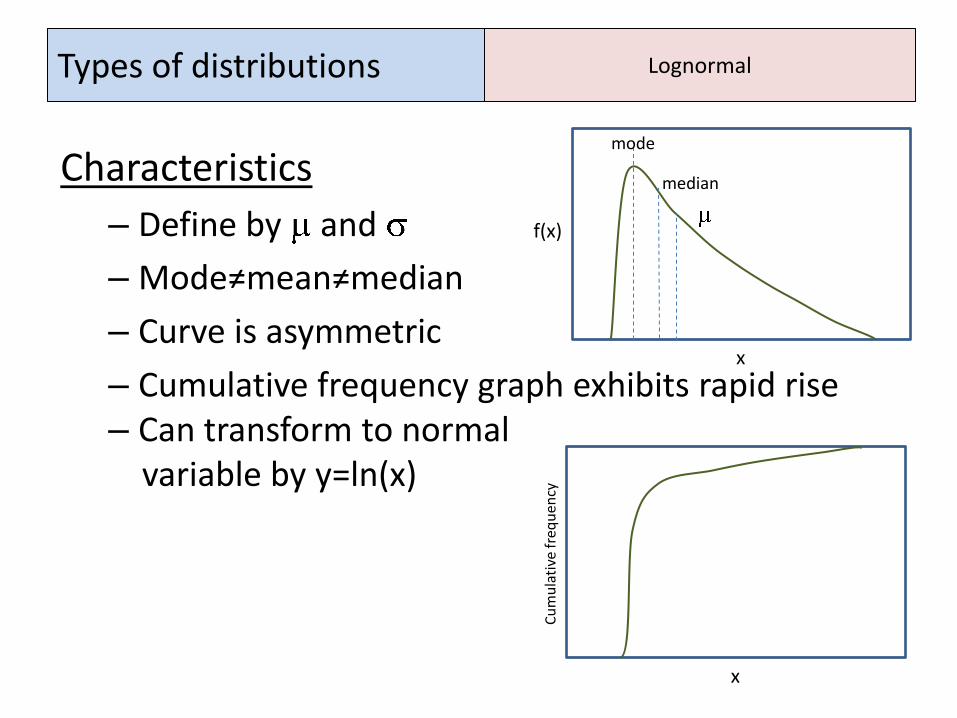
Characteristics
– Define by and
– Mode≠mean≠median
– Curve is asymmetric
– Cumulative frequency graph exhibits rapid rise– Can transform to normal
variable by y=ln(x)
Lognormal
x
Cu
mu
lati
ve f
req
uen
cy
x
f(x)
mode
median
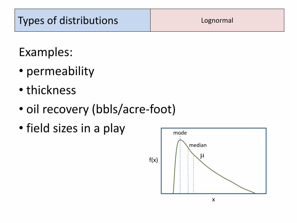
Types of distributions
Examples:
• permeability
• thickness
• oil recovery (bbls/acre-foot)
• field sizes in a play
Lognormal
x
f(x)
mode
median
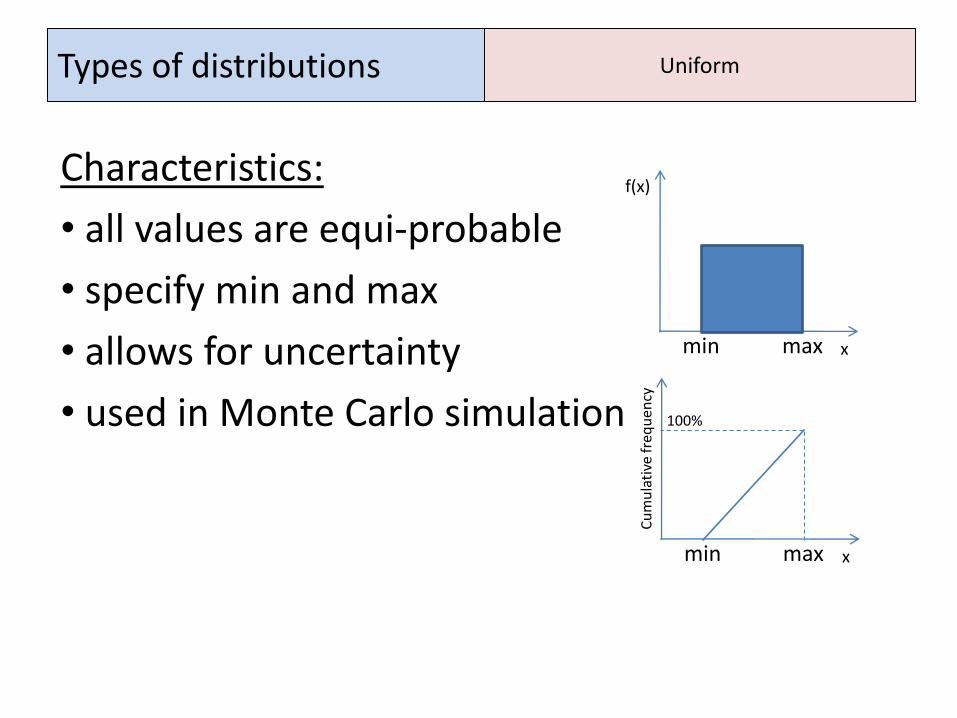
Types of distributions
Characteristics:
• all values are equi-probable
• specify min and max
• allows for uncertainty
• used in Monte Carlo simulation
Uniform
x
f(x)
min max
xmin max
Cu
mu
lati
ve f
req
uen
cy
100%

Types of distributions
Characteristics:
• all values are equi-probable
• specify min and max
• allows for uncertainty
• used in Monte Carlo simulation
Triangle
xmin max
Cu
mu
lati
ve f
req
uen
cy
100%
x
f(x)
L, low H, high
M, most likely

Types of distributions
Convert to cumulative frequency plot: • normalize to a 0 to 1 scale:
• Define m as:
• For x’ ≤ m, cumulative probability is given by:
• For x’ > m,
Triangle
LH
Lx'x
LH
LMm
x
f(x)
L, low H, high
M, most likely
m
2)x(
)x(P
m1
2)x1(
1)x(P
Types of distributions
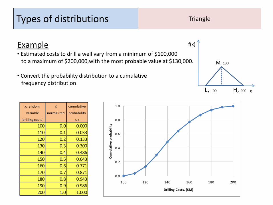
Example• Estimated costs to drill a well vary from a minimum of $100,000
to a maximum of $200,000,with the most probable value at $130,000.
• Convert the probability distribution to a cumulative frequency distribution
Triangle
x
f(x)
L, 100 H, 200
M, 130
x, random x' cumulative
variable normalized probability
(drilling costs) ≤ x
100 0.0 0.000
110 0.1 0.033
120 0.2 0.133
130 0.3 0.300
140 0.4 0.486
150 0.5 0.643
160 0.6 0.771
170 0.7 0.871
180 0.8 0.943
190 0.9 0.986
200 1.0 1.000
0.0
0.2
0.4
0.6
0.8
1.0
100 120 140 160 180 200
Cu
mu
lati
ve p
rob
abili
ty
Drilling Costs, ($M)

Types of distributions
Describes a stochastic process characterized by: 1. Only two outcomes can occur
2. Each trial is an independent event
3. The probability of each outcomes remains constant over repeated trials
4. Binomial probability equation is given by:
where
x = number of successes (0 ≤ x ≤ n)
n = total number of trials
p = probability of success on any given trial
and “the combination of n things taken x at a time”
Binomial
xn)p1(
xp
n
xC)x(P
)!xn(!x
!nn
xC
Types of distributions
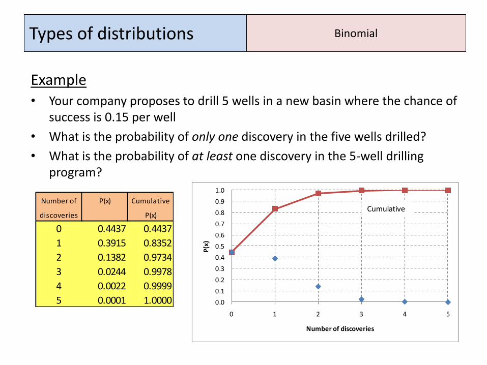
Example• Your company proposes to drill 5 wells in a new basin where the chance of
success is 0.15 per well
• What is the probability of only one discovery in the five wells drilled?
• What is the probability of at least one discovery in the 5-well drilling program?
Binomial
Number of P(x) Cumulative
discoveries P(x)
0 0.4437 0.4437
1 0.3915 0.8352
2 0.1382 0.9734
3 0.0244 0.9978
4 0.0022 0.9999
5 0.0001 1.0000 0.0
0.1
0.2
0.3
0.4
0.5
0.6
0.7
0.8
0.9
1.0
0 1 2 3 4 5
P(x
)
Number of discoveries
Cumulative
Types of distributions
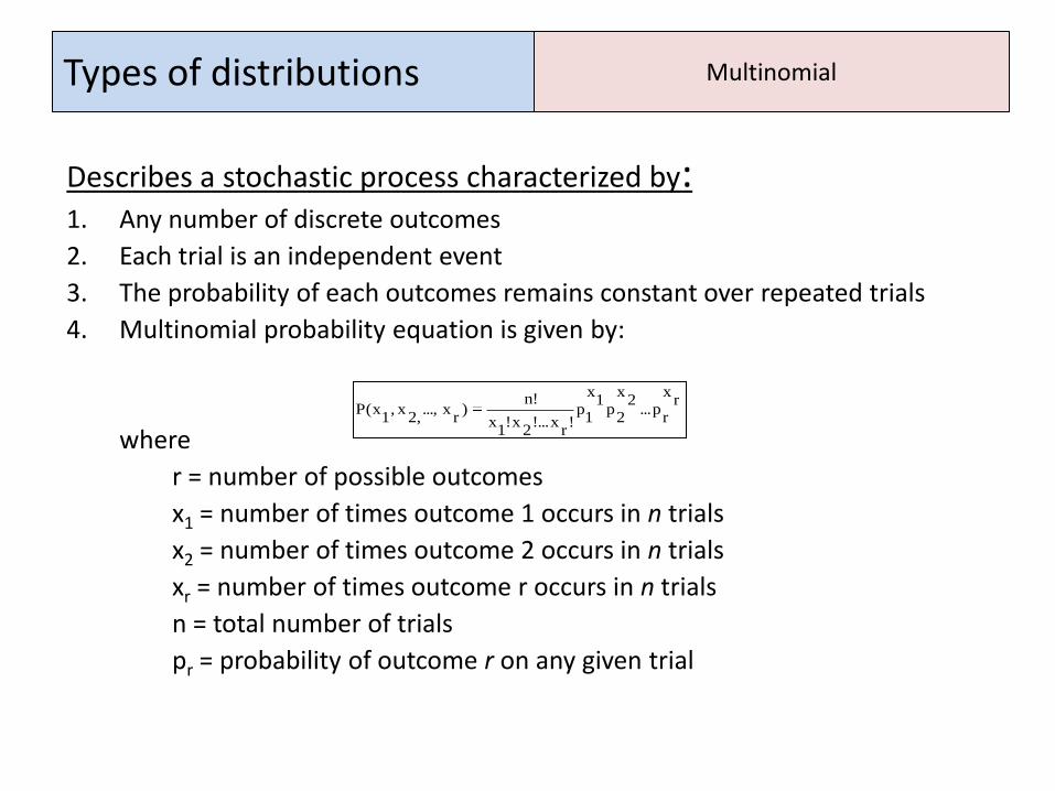
Describes a stochastic process characterized by: 1. Any number of discrete outcomes
2. Each trial is an independent event
3. The probability of each outcomes remains constant over repeated trials
4. Multinomial probability equation is given by:
where
r = number of possible outcomes
x1 = number of times outcome 1 occurs in n trials
x2 = number of times outcome 2 occurs in n trials
xr = number of times outcome r occurs in n trials
n = total number of trials
pr = probability of outcome r on any given trial
Multinomial
rx
rp...
2x
2p
1x
1p
!r
x!...2
x!1
x
!n)
rx...,
,2x,
1x(P
Types of distributions
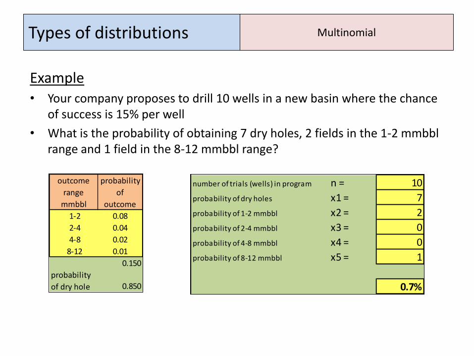
Example• Your company proposes to drill 10 wells in a new basin where the chance
of success is 15% per well
• What is the probability of obtaining 7 dry holes, 2 fields in the 1-2 mmbblrange and 1 field in the 8-12 mmbbl range?
Multinomial
outcome probability
range of
mmbbl outcome
1-2 0.08
2-4 0.04
4-8 0.02
8-12 0.01
0.150
probability
of dry hole 0.850
number of trials (wells) in program n = 10
probability of dry holes x1 = 7
probability of 1-2 mmbbl x2 = 2
probability of 2-4 mmbbl x3 = 0
probability of 4-8 mmbbl x4 = 0
probability of 8-12 mmbbl x5 = 1
0.7%

Types of distributions
Describes a stochastic process characterized by: 1. Any number of discrete outcomes2. Each trial is dependent on the previous event (sampling without
replacement)3. The probability of each outcomes remains constant over repeated trials4. Hypergeometric probability equation for two possible outcomes:
where n=number of trials di = number of successes in the sample space before the n trials xi = number of successes in n trials N = total number of elements in the sample space before the n trials Ca
b = the number of combinations of a things taken b at a time.
Hypergeometric
N
nC
1dN
xnC
1d
xC
)x(P

Types of distributions
Example• Our company has identified ten seismic anomalies of about equal size in a
new offshore area. In an adjacent area, 30% of the drilled structures were oil productive.
• If we drill 5 wells (test 5 anomalies) what is the probability of two discoveries?
Hypergeometric
number_sample n = 5
number_pop N = 10
population_s d1 = 3
sample_s x1 = 2
42%