Embed Size (px)
Citation preview

Basic Econometrics
Riccardo (Jack) Lucchetti
May 23, 2020

Foreword
This is a very basic course in econometrics, in that it only covers basic tech-niques, although I tried to avoid the scourge of over-simplification, so some mayfind it not so basic in style. What makes it perhaps a little different from othersyou find on the Net is that I made a few not-so-common choices.
1. Separating clearly the properties OLS has by construction from those ithas when interpreted as an estimator.
2. Using matrix algebra whenever possible.
3. Using asymptotic inference only.
Point number one is modelled after the ideas in the two great masterpieces,Davidson and MacKinnon (1993) and Davidson and MacKinnon (2004). I haveseveral reasons for this choice, but it is mainly a pedagogical one. The students Iam writing for are people who often don’t feel at ease with the tools of statisticalinference: they have learned the properties of estimators by heart, they are notsure they can read a test, find the concept of the distribution of a statistic a littleunclear (never mind asymptotic distributions), get confused between the vari-ance of an estimator and an estimator of the variance. In the best cases. Nevermind; no big deal.
There’s an awful lot you can say on the base tool in econometrics (OLS) evenwithout all this, and that’s good to know. Once a student has learned how tohandle OLS properly as a mere computational tool, the issues of its usage andinterpretation as an estimator and of how to read the associated test statisticscan be grasped more correctly. If you mix the two aspects too early, a beginneris prone to mistake properties of least squares that are true by construction forproperties that depend on some probabilistic assumptions.
Point number two is motivated by laziness. In my teaching career, I havefound that once students get comfortable with matrices, my workload halves. Ofcourse, it takes some initial sunk cost to convey properly ideas such as projec-tions and properties of quadratic forms, but the payoff is very handsome. Thisbook contains no systematic account of matrix algebra; we’re using just the ba-sics, so anything you find on the Net by googling “matrix algebra lecture notes”is probably good enough. However, let me recommend appendix A in Hansen(2019).
As for probability and statistics, I will only assume some familiarity with thevery basics: simple descriptive statistics and basic properties of probability, ran-dom variables and expectations. Chapter 2 contains a cursory treatment of theconcepts I will use later, but I wouldn’t recommend it as a general reference onthe subject. Its purpose is mainly to make the notation explicit and clarify a fewpoints. For example, I will avoid any kind of reference to maximum likelihoodmethods. For a more substantial read, it’s hard not to recommend, again, the
i

online material by Bruce Hansen: his “Probability and Statistics”, is availableonline at https://www.ssc.wisc.edu/~bhansen/probability/.
I don’t think I have to justify point number three. I am writing this in 2020,when typical data sets have hundreds, if not thousands observations and no-body would ever dream of running any kind of inferential procedure with lessthan 50 data points. Apart from OLS, there is no econometric technique in actualuse that does not depend vitally on asymptotics, so I guess that readers shouldget familiar with the associated concepts if there is a remote chance that thiswill not be put them off econometrics completely. The t test, the F tests and,in general, all kinds of degrees-of-freedom corrections are ad-hockeries of thepast; unbiasedness is overrated. Get over it.
I promise I’ll try to be respectful of the readers and don’t treat them like id-iots. I assume that if you’re reading this, you want to know more than you doabout econometrics, but this doesn’t give me the right to assume that you needto be taken by the hand and treated like an 11-year-old.
Finally, a word of gratitude. A book like this is akin to a software project, andthere’s always one more bug to fix. So, I’d like to thank first all my students whohelped me eradicate quite a few. Then, my colleagues Stefano Fachin, FrancescaMariani, Giulio Palomba, Luca Pedini, Matteo Picchio and Claudia Pigini formaking many valuable suggestions. Needless to say, the remaining shortcom-ings are all mine. Claudia also allowed me to grab a few things from her slideson IV estimation, so thanks for that too. If you want to join the list, please sendme bug reports and feature requests. Also, I’m not an English native speaker (Isuppose it shows). So, Anglophones of the world, please correct me wheneverneeded.
The structure of this book is as follows: chapter 1 explores the propertiesof OLS as a descriptive statistic. Inference comes into play at chapter 2 withsome general concepts, while their application to OLS is the object of chapter3. Chapters 4 and 5 contain extensions of the basic model for cross-sectionaland time-series datasets, respectively. Finally, chapter 6 deals with instrumentalvariable estimation. Each chapter has an appendix, named “Assorted results”,where I discuss some of the material I use during the chapter in a little moredetail.
In some cases, I will use a special format forshort pieces of texts, like this. They contain ex-tra stuff that I consider interesting, but not in-
dispensable for the overall comprehension ofthe main topic.
This work is licensed under a Creative Commons“Attribution-ShareAlike 3.0 Unported” license.
ii

Contents
Foreword . . . . . . . . . . . . . . . . . . . . . . . . . . . . . . . . . . . . . . i
1 OLS: algebraic and geometric properties 11.1 Models . . . . . . . . . . . . . . . . . . . . . . . . . . . . . . . . . . . . 11.2 The average . . . . . . . . . . . . . . . . . . . . . . . . . . . . . . . . . 31.3 OLS as a descriptive statistic . . . . . . . . . . . . . . . . . . . . . . . 6
1.3.1 OLS on a dummy variable . . . . . . . . . . . . . . . . . . . . . 61.3.2 The general case . . . . . . . . . . . . . . . . . . . . . . . . . . 101.3.3 Collinearity and the dummy trap . . . . . . . . . . . . . . . . . 131.3.4 Nonlinearity . . . . . . . . . . . . . . . . . . . . . . . . . . . . . 15
1.4 The geometry of OLS . . . . . . . . . . . . . . . . . . . . . . . . . . . . 161.4.1 Projection matrices . . . . . . . . . . . . . . . . . . . . . . . . . 181.4.2 Measures of fit . . . . . . . . . . . . . . . . . . . . . . . . . . . . 20
1.5 The Frisch-Waugh theorem . . . . . . . . . . . . . . . . . . . . . . . . 231.6 An example . . . . . . . . . . . . . . . . . . . . . . . . . . . . . . . . . 251.A Assorted results . . . . . . . . . . . . . . . . . . . . . . . . . . . . . . . 27
1.A.1 Matrix differentiation rules . . . . . . . . . . . . . . . . . . . . 281.A.2 Vector spaces . . . . . . . . . . . . . . . . . . . . . . . . . . . . 291.A.3 Rank of a matrix . . . . . . . . . . . . . . . . . . . . . . . . . . . 301.A.4 Rank and inversion . . . . . . . . . . . . . . . . . . . . . . . . . 311.A.5 Step-by-step derivation of the sum of squares function . . . . 321.A.6 Numerical collinearity . . . . . . . . . . . . . . . . . . . . . . . 331.A.7 Definiteness of square matrices . . . . . . . . . . . . . . . . . 341.A.8 A few more results on projection matrices . . . . . . . . . . . 341.A.9 Proof of equation (1.21) . . . . . . . . . . . . . . . . . . . . . . 36
2 Some statistical inference 392.1 Why do we need statistical inference? . . . . . . . . . . . . . . . . . . 392.2 A crash course in probability . . . . . . . . . . . . . . . . . . . . . . . 40
2.2.1 Probability and random variables . . . . . . . . . . . . . . . . 412.2.2 Independence and conditioning . . . . . . . . . . . . . . . . . 432.2.3 Expectation . . . . . . . . . . . . . . . . . . . . . . . . . . . . . 442.2.4 Conditional expectation . . . . . . . . . . . . . . . . . . . . . . 46
2.3 Estimation . . . . . . . . . . . . . . . . . . . . . . . . . . . . . . . . . . 47
iii
2.3.1 Consistency . . . . . . . . . . . . . . . . . . . . . . . . . . . . . 482.3.2 Asymptotic normality . . . . . . . . . . . . . . . . . . . . . . . 50
2.4 Hypothesis Testing . . . . . . . . . . . . . . . . . . . . . . . . . . . . . 552.4.1 The p-value . . . . . . . . . . . . . . . . . . . . . . . . . . . . . 59
2.5 Identification . . . . . . . . . . . . . . . . . . . . . . . . . . . . . . . . 612.A Assorted results . . . . . . . . . . . . . . . . . . . . . . . . . . . . . . . 63
2.A.1 Jensen’s lemma . . . . . . . . . . . . . . . . . . . . . . . . . . . 632.A.2 The normal and χ2 distributions . . . . . . . . . . . . . . . . . 642.A.3 Gretl script to reproduce example 2.5 . . . . . . . . . . . . . . 68
3 Using OLS as an inferential tool 693.1 The regression function . . . . . . . . . . . . . . . . . . . . . . . . . . 693.2 Main statistical properties of OLS . . . . . . . . . . . . . . . . . . . . 72
3.2.1 Consistency . . . . . . . . . . . . . . . . . . . . . . . . . . . . . 723.2.2 Asymptotic normality . . . . . . . . . . . . . . . . . . . . . . . 73
3.3 Specification testing . . . . . . . . . . . . . . . . . . . . . . . . . . . . 753.3.1 Tests on a single coefficients . . . . . . . . . . . . . . . . . . . 753.3.2 More general tests . . . . . . . . . . . . . . . . . . . . . . . . . 77
3.4 Example: reading the output of a software package . . . . . . . . . . 793.4.1 The top table: the coefficients . . . . . . . . . . . . . . . . . . 803.4.2 The bottom table: other statistics . . . . . . . . . . . . . . . . 82
3.5 Exogeneity and causal effects . . . . . . . . . . . . . . . . . . . . . . . 833.6 Restricted Least Squares and hypothesis testing . . . . . . . . . . . . 84
3.6.1 Two alternative test statistics . . . . . . . . . . . . . . . . . . . 873.7 Prediction . . . . . . . . . . . . . . . . . . . . . . . . . . . . . . . . . . 903.8 The so-called “omitted-variable bias” . . . . . . . . . . . . . . . . . . 923.A Assorted results . . . . . . . . . . . . . . . . . . . . . . . . . . . . . . . 95
3.A.1 Consistency of σ2 . . . . . . . . . . . . . . . . . . . . . . . . . . 953.A.2 The Gauss-Markov theorem . . . . . . . . . . . . . . . . . . . . 953.A.3 Derivation of RLS . . . . . . . . . . . . . . . . . . . . . . . . . . 973.A.4 Asymptotic properties of the RLS estimator . . . . . . . . . . 99
4 Diagnostic testing in cross-sections 1014.1 Diagnostics for the conditional mean . . . . . . . . . . . . . . . . . . 102
4.1.1 The RESET test . . . . . . . . . . . . . . . . . . . . . . . . . . . 1024.1.2 Interactions and the Chow test . . . . . . . . . . . . . . . . . . 104
4.2 Heteroskedasticity and its consequences . . . . . . . . . . . . . . . . 1094.2.1 If Σwere known . . . . . . . . . . . . . . . . . . . . . . . . . . . 1104.2.2 Robust estimation . . . . . . . . . . . . . . . . . . . . . . . . . 1124.2.3 White’s test . . . . . . . . . . . . . . . . . . . . . . . . . . . . . . 1144.2.4 So, in practice. . . . . . . . . . . . . . . . . . . . . . . . . . . . . 117
4.A Assorted results . . . . . . . . . . . . . . . . . . . . . . . . . . . . . . . 1194.A.1 Proof of equation (4.2) . . . . . . . . . . . . . . . . . . . . . . . 119
iv
4.A.2 Proof that full interactions are equivalent to split-sampleestimation . . . . . . . . . . . . . . . . . . . . . . . . . . . . . . 120
4.A.3 Proof that GLS is more efficient than OLS . . . . . . . . . . . . 1224.A.4 The bootstrap . . . . . . . . . . . . . . . . . . . . . . . . . . . . 122
5 Dynamic Models 1255.1 Dynamic regression . . . . . . . . . . . . . . . . . . . . . . . . . . . . 1255.2 Manipulating difference equations . . . . . . . . . . . . . . . . . . . . 129
5.2.1 The lag operator . . . . . . . . . . . . . . . . . . . . . . . . . . . 1305.2.2 Dynamic multipliers . . . . . . . . . . . . . . . . . . . . . . . . 1325.2.3 Interim and long-run multipliers . . . . . . . . . . . . . . . . . 135
5.3 Inference on OLS with time-series data . . . . . . . . . . . . . . . . . 1365.3.1 Martingale differences . . . . . . . . . . . . . . . . . . . . . . . 1365.3.2 Testing for autocorrelation and the general-to-specific ap-
proach . . . . . . . . . . . . . . . . . . . . . . . . . . . . . . . . 1385.4 An example, perhaps? . . . . . . . . . . . . . . . . . . . . . . . . . . . 1405.5 The ECM representation . . . . . . . . . . . . . . . . . . . . . . . . . . 1425.6 Hypothesis tests on the long-run multiplier . . . . . . . . . . . . . . 1455.7 Forecasting and Granger causality . . . . . . . . . . . . . . . . . . . . 1475.A Assorted results . . . . . . . . . . . . . . . . . . . . . . . . . . . . . . . 152
5.A.1 Inverting polynomials . . . . . . . . . . . . . . . . . . . . . . . 1525.A.2 Basic concepts on stochastic processes . . . . . . . . . . . . . 1535.A.3 Why martingale difference sequences are serially uncorre-
lated . . . . . . . . . . . . . . . . . . . . . . . . . . . . . . . . . 1555.A.4 From ADL to ECM . . . . . . . . . . . . . . . . . . . . . . . . . 156
6 Instrumental Variables 1596.1 Examples . . . . . . . . . . . . . . . . . . . . . . . . . . . . . . . . . . . 159
6.1.1 Measurement error . . . . . . . . . . . . . . . . . . . . . . . . . 1596.1.2 Simultaneous equation systems . . . . . . . . . . . . . . . . . 161
6.2 The IV estimator . . . . . . . . . . . . . . . . . . . . . . . . . . . . . . . 1636.2.1 The generalised IV estimator . . . . . . . . . . . . . . . . . . . 1646.2.2 The instruments . . . . . . . . . . . . . . . . . . . . . . . . . . 166
6.3 An example with real data . . . . . . . . . . . . . . . . . . . . . . . . . 1686.4 The Hausman test . . . . . . . . . . . . . . . . . . . . . . . . . . . . . . 1696.5 Two-stage estimation . . . . . . . . . . . . . . . . . . . . . . . . . . . . 172
6.5.1 The control function approach . . . . . . . . . . . . . . . . . . 1756.6 The examples, revisited . . . . . . . . . . . . . . . . . . . . . . . . . . 177
6.6.1 Measurement error . . . . . . . . . . . . . . . . . . . . . . . . . 1776.6.2 Simultaneous equation systems . . . . . . . . . . . . . . . . . 178
6.7 Are my instruments OK? . . . . . . . . . . . . . . . . . . . . . . . . . . 1796.7.1 The Sargan test . . . . . . . . . . . . . . . . . . . . . . . . . . . 1806.7.2 Weak instruments . . . . . . . . . . . . . . . . . . . . . . . . . 182
6.A Assorted results . . . . . . . . . . . . . . . . . . . . . . . . . . . . . . . 186
v

6.A.1 Asymptotic properties of the IV estimator . . . . . . . . . . . 1866.A.2 Proof that OLS is more efficient than IV . . . . . . . . . . . . . 1886.A.3 Covariance matrix for the Hausman test (scalar case) . . . . . 1886.A.4 Hansl script for the weak instrument simulation study . . . . 189
Bibliography 191
vi
Chapter 1
OLS: algebraic and geometricproperties
1.1 Models
I won’t even attempt to give the reader an account of the theory of econometricmodelling. For our present purposes, suffice it to say that we econometricianslike to call a model a mathematical description of something, that doesn’t aimat being 100% accurate, but still, hopefully, useful.1
We have a quantity of interest, also called the dependent variable, whichwe observe more than once: a collection of numbers y1, y2, . . . , yn , where n is thesize of our data set. These numbers can be anything that can be given a coherentnumerical representation; in this course, however, we will confine ourselves tothe case where the i -th observation yi is a real number. So for example, we couldrecord the income for n individuals, the export share for n firms, the inflationrate for a given country at n points in time.
Now suppose that, for the same data points, we also have a vector of k el-ements containing auxiliary data possibly helpful in better understanding thedifferences between the yi s; we call these explanatory variables,2 or xi in sym-bols.3 To continue the previous examples, xi may include a numerical descrip-tion of the individuals we recorded the income of (such as age, gender, educa-tional attainment and so on), or characteristics of the firms we want to study theexport propensity for (size, turnover, R&D expenditure and so on), or the con-ditions of the economy at the time the inflation rate was recorded (interest rate,level of output, and so forth).
What we call a model is a formula like the following:
yi ' m(xi )
1“All models are wrong, but some are useful” (G. E. P. Box).2Terminology is very much field-specific here; statisticians traditionally tend to use the term
covariates, while people from the machine learning community like the word features.3I will almost always use boldface symbols to indicate vectors.
1
2 CHAPTER 1. OLS: ALGEBRAIC AND GEOMETRIC PROPERTIES
where we implicitly assume that if xi is not too different from x j , then we shouldexpect yi to be broadly close to y j : if we pick two people of the same age, withthe same educational level and many other characteristics in common we wouldexpect that their income should be roughly the same. Of course this won’t betrue in all cases (in fact, chances are that this will never be true exactly), buthopefully our model won’t lead us to catastrophic mistakes.
The reason why we want to build models is that, once the function m(·) isknown, it becomes possible to ask ourselves interesting questions by inspect-ing the characteristics of that function. So for example, if it turned out that theexport share of a firm is increasing in the expenditure in R&D, we may make con-jectures about the reasons why it should be so, look for some economic theorythat could explain the result, and wonder if one could improve export competi-tiveness by giving the firms incentives to do research.
Moreover, the door is open to forecasting: given the characteristics of a hy-pothetical firm or individual, the model makes it possible to guess what theirexport share or income (respectively) should be. I don’t think I have to convincethe reader of how useful this could be in practice.
Of course, we will want to build our model in the best possible way. In otherwords, our aim will be choosing the function m(·) according to some kind ofoptimality criterion. This is what the present course is about.
But there’s more: as we will see, building an optimal model is impossible ingeneral. At most, we may hope to build the best possible model for the datathat we have available. Of course, there is no way of knowing if the model webuilt, that perhaps works rather well with our data, will keep working equallywell with new data. Imagine you built a model for the inflation rate in a countrywith monthly data from January 2000 to December 2017. It may well be that yourmodel performs (or, as we say, “fits the data”) very well for that period, but whatguarantee do you have that it will keep doing so in 2018, or in the more distantfuture? The answer is: you have none. But still, this is something that we’d like todo; our mind has a natural tendency to generalise, to infer, to extrapolate. Andyet, there is no logical compelling basis for proving that it’s a good idea to doso.4 The way out is framing the problem in a probabilistic setting, and this is thereason why econometrics is so intimately related with probability and statistics.
For the moment, we’ll start with the problem of choosing m(·) in a very sim-ple case, that is when we have no extra information xi . In this case, the functionbecomes a constant:
yi ' m(xi ) = m
and the problem is very much simplified, because it means we have to pick anumber m in some optimal way, given the data y1, y2, . . . , yn . In other words, wehave to find a function of the data which returns the number m. Of course, afunction of the data is what we call a statistic. In the next section, I will prove
4‘The philosophically inclined reader may at this point google for “Bertrand Russel’s turkey”.
1.2. THE AVERAGE 3
that the statistic we’re looking for is, in this case, the average of the yi s, that isY = 1
n
∑ni=1 yi .
1.2 The average
What is a descriptive statistic? It is a function of the data which synthesises aparticular feature of interest of the data; of course, the more informative, thebetter. The idea behind descriptive statistics is more or less: we have some dataon some real-world phenomenon; our data set, unfortunately, is too “large”, andwe don’t have time/can’t/don’t feel like going through the whole thing. Hence,we are looking for a function of these data to tell us what we want, without beingbothered with unnecessary details.
The most obvious example of a descriptive statistic is, of course, the sampleaverage. Let’s stick our observations y1, y2, . . . , yn into a column vector y; thesample average is nothing but
Y = 1
n
n∑i=1
yi = 1
nι′y, (1.1)
where ι is a column vector full of ones. The “sum” notation is probably morefamiliar to most readers; I prefer the matrix-based one not only because I findit more elegant, but also because it’s far easier to generalise. The nice featureof the vector ι is that its inner product with any conformable vector x yields thesum of the elements of x.5
We use averages all the time. Why is the average so popular? As I said, we’relooking for a descriptive statistic m, as a synthesis of the information containedin our data set.
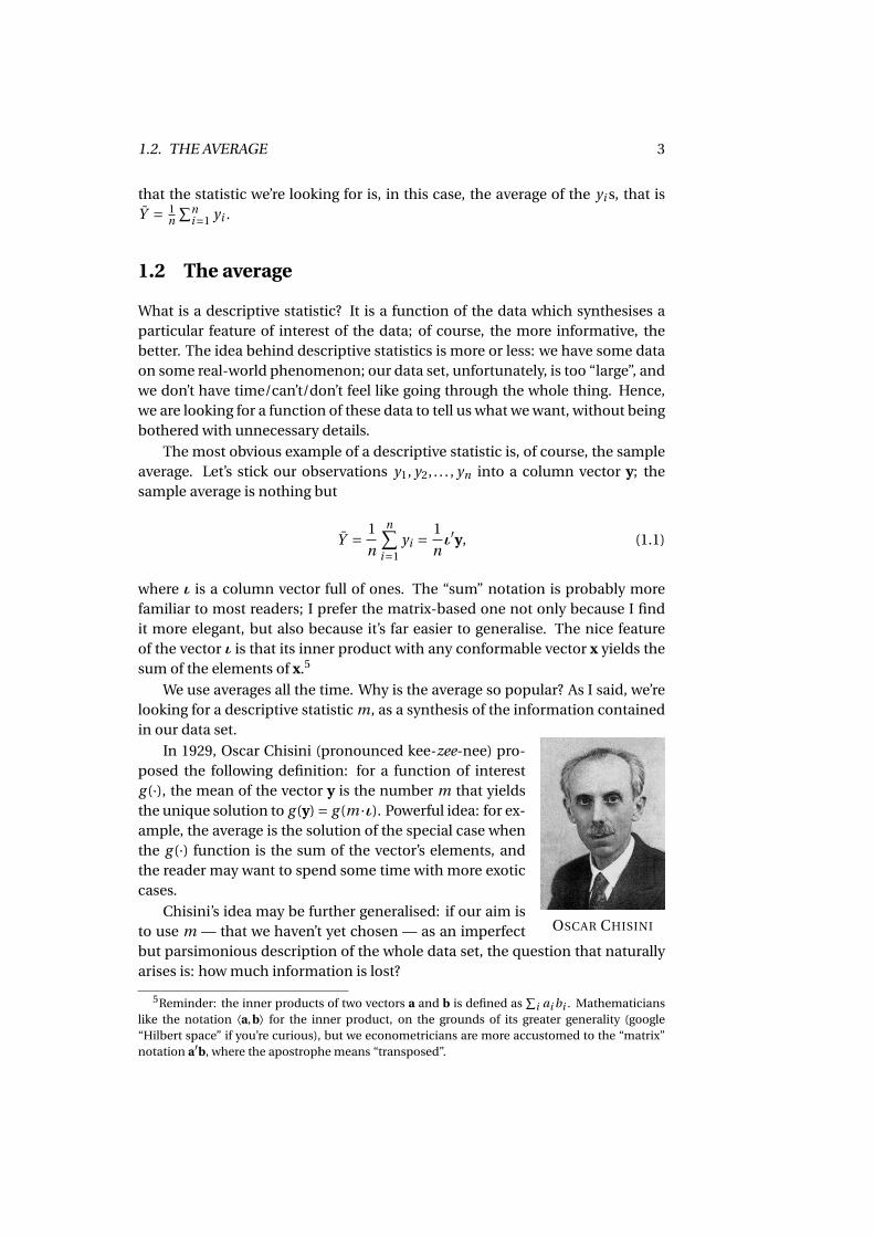
OSCAR CHISINI
In 1929, Oscar Chisini (pronounced kee-zee-nee) pro-posed the following definition: for a function of interestg (·), the mean of the vector y is the number m that yieldsthe unique solution to g (y) = g (m ·ι). Powerful idea: for ex-ample, the average is the solution of the special case whenthe g (·) function is the sum of the vector’s elements, andthe reader may want to spend some time with more exoticcases.
Chisini’s idea may be further generalised: if our aim isto use m — that we haven’t yet chosen — as an imperfectbut parsimonious description of the whole data set, the question that naturallyarises is: how much information is lost?
5Reminder: the inner products of two vectors a and b is defined as∑
i ai bi . Mathematicianslike the notation ⟨a,b⟩ for the inner product, on the grounds of its greater generality (google“Hilbert space” if you’re curious), but we econometricians are more accustomed to the “matrix”notation a′b, where the apostrophe means “transposed”.
4 CHAPTER 1. OLS: ALGEBRAIC AND GEOMETRIC PROPERTIES
If all we knew, for a given data set, was m, what could we say about eachsingle observation? If we lack any more information, the most sensible thing tosay is that, for a generic i , yi should more or less be m. Consider the case ofA. S. Tudent, who belongs to a class for which the “typical” grade in economet-rics is 23;6 the most sensible answer we could give to the question “What was thegrade that A. S. Tudent got in econometrics?” would be “Around 23, I guess”. Ifthe actual grade that A. S. got were in fact 23, OK. Otherwise, we could measureby how much we were wrong by taking the difference between the actual gradeand our guess, ei = yi −m. We call these quantities the residuals; the vector ofresiduals is, of course, e = y−ι ·m.
In the ideal case, using m to summarise the data should entail no informa-tion loss at all, and the difference between yi and m should be 0 for all i (all stu-dents got 23). If it weren’t so, we may measure how well m does its job throughthe size of the residuals. Let’s define a function, called loss function, which mea-sures the cost we incur because of the information loss.
L(m) =C [e(m)]
In principle, there are not many properties such a function should be assumedto have. It seems reasonable that C (0) = 0:7 if all the residuals are 0, no approxi-mation errors occur and the cost is nil. Another reasonable idea is C (e) ≥ 0: youcan’t gain from a mistake.8 Apart from this, there is not very much you can say:the L(·) function cannot be assumed to be convex, or symmetric, or anythingelse. It depends on the context.
Whatever the shape of this function, however, we’ll want to choose m so thatis L(m) as small as possible. In math-speak: for a given problem, we can writedown the loss function and choose the statistic which minimises it. In formulae:
m = Argminm∈R
L(m) = Argminm∈R
C (y−ι ·m) (1.2)
The hat ( ˆ ) on m indicates that, among all possible real numbers, we are choos-ing the one that minimises our loss function.
In practice, by finding the minimum of the L(·) function for a given prob-lem, we can be confident that we are using our data in the best possible way.At this point, the first thing that crosses a reasonable person’s mind is “How doI choose L(·)? I mean, what does it look like? I can’t just google ‘loss function’,can I?”. True. Apart from extraordinary cases when the loss function is a natu-ral consequence of the problem itself, writing down its exact mathematical formmay be complicated. What does the L(m) function look like for the grades ineconometrics of our hypothetical class? Hard to say.
6Note for international readers: in the Italian academic systems, which is what I’m used to,grades go from 18 (barely pass) to 30 (full marks).
7I use a boldface 0 to indicate a vector full of zeros, as in 0 ·ι= 0.8Warning: the converse is not necessarily true. It’s possible that the cost is nil even with non-
zero errors. For example, in some contexts “small” error may be irrelevant.
1.2. THE AVERAGE 5
Moreover, we often must come up with a summary statistic without know-ing in advance what it will be used for. Obviously, in these cases finding a one-size-fits-all optimal solution is downright impossible. We have to make do withsomething that is not too misleading. A possible choice is
L(m) =n∑
i=1(yi −m)2 = (y−ι ·m)′(y−ι ·m) = e′e (1.3)
The above criterion is a function of m based on the sum of squared residuals,that enjoys several desirable properties. Not only it’s simple to manipulate al-gebraically: it’s symmetric and convex, so that positive and negative residualsare penalised equally, and large errors are more costly than small ones. It’s notunreasonable to take this loss function as an acceptable approximation. More-over, this choice makes it extremely easy to solve the associated minimisationproblem.
Minimising L(m) with respect to m leads to the so-called least squares prob-lem. All is needed to find the minimum in (1.3) is taking the derivative of L(m)with respect to m;
dL(m)
dm=
n∑i=1
d(yi −m
)2
dm=−2
n∑t=1
(yi −m
)The derivative must be 0 for a minimum, so that
n∑i=1
(yi −m
)= 0
which in turn implies
n ·m =n∑
t=1yi
and therefore m = n−1 ∑ni=1 yi = Y . The reader is invited to verify that m is
indeed a minimum, by checking that the second derivative d2L(m)dm2 is positive.
Things are even smoother in matrix notation:
L(m) = (y−ιm)′(y−ιm) = y′y−2m ·ι′y+m2ι′ι,
so the derivative is
dL(m)
dm=−2ι′y+2m ·ι′ι=−2ι′(y−ιm) = 0
whenceι′y = (ι′ι) ·m =⇒ m = (ι′ι)−1ι′y = Y
because of course ι′ι = n. The value of L(m) at the minimum, that is L(m) =e′e = ∑n
i=1(yi − Y )2 is a quantity that in this case we call deviance, but that wewill more often call SSR, as in Sum of Squared Residuals.
6 CHAPTER 1. OLS: ALGEBRAIC AND GEOMETRIC PROPERTIES
The mathematically sophisticated way to say the same is
m = Argminm∈R
L(m);
you read the above as: m with a hat on is that number that you find if you choose,among all real numbers, the one that makes the function L(m) as small as pos-sible.
The argument above, which leads to choosing the average as an optimalsummary is, in fact, much more general than it may seem: many of the descrip-tive statistics we routinely use are special cases of the average, where the data yare subject to some preliminary transformation.
In practice: the average of z, where zi = h(yi ) can be very informative, if wechoose the function h(·) wisely. The variance is the most obvious example: thesample variance9 is just the average of zi = (yi − Y )2, which measures how far yi
is from Y .Things get even more interesting when we express a frequency as an average:
define the event E = yi ∈ A, where A is some subset of the possible values foryi ; now define the variable zi = I(yi ∈ A), where I(·) is the so-called “indicatorfunction”, that gives 1 when its argument is true and 0 when false. Evidently, theaverage of the zi , Z , is the relative frequency of E . I’m sure you can come upwith more examples.
1.3 OLS as a descriptive statistic
1.3.1 OLS on a dummy variable
Now let’s bring the explanatory variables xi back in. For the moment, let’s con-sider the special case where xi is a one-element vector, that is a scalar.
A possible way to check if yi and xi are related to each other is to see if yi is“large” or “small” when xi is “large” or “small”. Define
zi = (yi − Y )(xi − X )
which is, in practice, a sort of indicator of “matching magnitudes”: zi is positivewhen yi > Y and xi > X (both are “large”) or when yi < Y and xi < X (bothare “small”); on the contrary, zi is negative when magnitudes don’t match. Asis well known, the average of zi is known as covariance; but this is just boringelementary statistics.
The reason why I brought this up is to highlight the main problem with co-variance (and correlation, that is just covariance rescaled so that it’s guaranteedto be between -1 and 1): it’s a symmetric concept. The variables yi and xi aretreated equally: the covariance between yi and xi is by construction the same as
9I’m not applying the “degrees of freedom correction”; I don’t see why I should, as long I’musing the variance as a descriptive statistic.
1.3. OLS AS A DESCRIPTIVE STATISTIC 7
between xi and yi . On the contrary, we often like to think in terms of yi = m(xi ),because what we have in mind is an interpretation where yi “depends” on xi ,and not the other way around.10 This is why we call yi the dependent variableand xi the explanatory variable. In this context, it’s rather natural to see whathappens if you split y into several sub-vectors, according to the values that xi
takes. In a probabilistic context, we’d call this conditioning (see section 2.2.2).Simple example: suppose our vector y includes observations on n people,
with nm males and n f = n−nm females. The information on gender is in a vari-able xi , that equals 1 for males and 0 for females. As is well known, a 0/1 variablemay be called “binary”, “Boolean”, “dichotomic”, but we econometricians tradi-tionally call it a dummy variable.
Common sense suggests that, if we take into account the information wehave on gender, the average by gender will give us a data description whichshould be slightly less concise than overall average (since we’re using two num-bers instead of one), but certainly not less accurate. Evidently, we can define
Ym =∑
xi=1 yi
nm= Sm
nmY f =
∑xi=0 yi
n f= S f
n f
where Sm and S f are the sums of yi for males and females, respectively.Now, everything becomes more elegant and exciting if we formalise the prob-
lem in a similar way to what we did with the average. We would like to use in thebest possible way the information (that we assume we have) on the gender of thei -th individual. So, instead of summarising the data by a number, we are goingto use a function, that is something like
m(xi ) = mm · xi +m f · (1−xi )
which evidently equals mm for men (since xi = 1) and m f for women (since xi =0). Our summary will be a rule giving us ‘representative’ values of yi accordingto xi .
Let’s go back to our definition of residuals as approximation errors: in thiscase, you clearly have that ei ≡ yi −m(xi ), and therefore
yi = mm xi +m f (1−xi )+ei (1.4)
Equation (1.4) is a simple example of an econometric model. The numberyi is split into two additive components: a systematic part, that depends on thevariable xi (a linear function of xi , to be precise), plus a remainder term, that wejust call the residual for now. In this example, m(xi ) = mm xi +m f (1−xi ).
10I’m being deliberately vague here: in everyday speech, saying that A depends on B may meanmany things, not necessarily consistent. For example, “dependence” may not imply a cause-effectlink. This problem is much less trivial than it seems at first sight, and we’ll leave it to professionalepistemologists.
8 CHAPTER 1. OLS: ALGEBRAIC AND GEOMETRIC PROPERTIES
It is convenient to rewrite (1.4) as
yi = m f + (mm −m f )xi +ei =[
1 xi][
m f
mm −m f
]+ei
so we can use matrix notation, which is much more compact and elegant
y = Xβ+e, (1.5)
where
β =[
m f
mm −m f
]=
[β1
β2
]and X is a matrix with n rows and 2 columns; the first column is ι and the secondone is x. The i -th row of X is [1,1] if the corresponding individual is male and[1,0] otherwise. To be explicit:
y1
y2...
yn−1
yn
=
1 x1
1 x2...
...1 xn−1
1 xn
[β1
β2
]+
e1
e2...
en−1
en
Therefore, the problem of choosing mm and m f optimally is transformed
into the problem of finding the vector β that minimises the loss function e′e.The solution is not difficult: find the solutions to11
d
dβe′e = d
dβ(y−Xβ)′(y−Xβ) = d
dβ(y′y−2β′X′y+β′X′Xβ) = 0
By using the well-known12 rules for matrix differentiation, you have
X′y = X′X · β (1.6)
What we have to do now is solve equation (1.6) for β. The solution is uniqueif X′X is invertible (if you need a refresher on matrix inversion, and related mat-ters, subsection 1.A.3 is for you):
β = (X′X
)−1 X′y. (1.7)
Equation (1.7) is the single most important equation in this book, and this iswhy I framed it into a box. The vector β is defined as the vector that minimisesthe sum of squared residuals:
β = Argminβ∈Rk
e′e,
11Need I remind the reader of the rule for transposing a matrix product, that is (AB)′ = B ′A′?Obviously not.
12Not so well-known, maybe? Jump to subsection 1.A.1.
1.3. OLS AS A DESCRIPTIVE STATISTIC 9
and the expression in equation (1.7) turns the implicit definition into an explicitformula that you can use to calculate β.
The coefficients β obtained from (1.7) are known as OLS coefficients, or OLSstatistic, from Ordinary Least Squares.13 A very common idiom that economistsuse when referring to the calculation of OLS is “regressing y on X”. The usage ofthe word “regression” here might seem odd, but will be justified in chapter 3.
The “hat” symbol has exactly the same meaning as in eq. (1.2): of all thepossible choices for β, we pick the one that makes eq. (1.6) true, and thereforeminimises the associated loss function e′e. The vector
y = Xβ
is our approximation to y. The term we normally use for the elements of y arethe fitted values: the closer they are to y, the better we say that the model fitsthe data.
In this example, a few simple calculations suffice to show that
X′X =[
n nm
nm nm
]X′y =
[ ∑ni=1 yi∑
xi=1 yi
]=
[Sm +S f
Sm
]where Sm = ∑
xi=1 yi and S f = ∑xi=0 yi : the sums of yi for males and females,
respectively. By using the standard rule for inverting (2× 2) matrices, which Iwill also assume known,14
(X′X)−1 = 1
nmn f
[nm −nm
−nm n
]so that
β = 1
nmn f
[nm −nm
−nm n
][Sm +S f
Sm
]= 1
nmn f
[nmS f
n f Sm −nmS f
]and finally
β = S f
n f
Smnm
− S f
n f
=[
Y f
Ym − Y f
]so that our model is:
yi = Y f +[Ym − Y f
]xi
and it’s easy to see that the fitted value for males (xi = 1) is Ym , while the one forthe females (xi = 0) is Y f .
Once again, opting for a quadratic loss function (e′e) delivers a solution con-sistent with common sense. In this case, however, our approximate descriptionof the vector y uses a function whose parameters are the statistics we are inter-ested in.
13Why “ordinary”? Well, because there are more sophisticated variants, so we call these “ordi-nary” as in “not extraordinary”. We’ll see one of those variants in section 4.2.1.
14If you’re in trouble, go to subsection 1.A.3
10 CHAPTER 1. OLS: ALGEBRAIC AND GEOMETRIC PROPERTIES
1.3.2 The general case
In reading the previous subsection, the discerning reader will have noticed that,in fact, the assumption that x is a dummy variable plays a very marginal rôle.There is no reason why the equation m(xi ) = β1 +β2xi should not hold whenxi contains generic numeric data. The solution to the problem remains un-changed; clearly, the vector β will not contain the averages by sub-samples, butthe fact that the loss function is minimised by β = (X′X)−1X′y keeps being true.
Example 1.1Suppose that
y =
132301
x =
432511
The reader is invited to check that15
X′X =[
6 1616 56
]⇒ (X′X)−1 =
[0.7 −0.2
−0.2 3/40
]X′y =
[1033
]and therefore
β =[
0.40.475
]y =
2.31.8251.3452.7750.8750.875
e =
−1.31.175
0.650.225
−0.8750.125
Hence, the function m(xi ) minimising the sum of squared residuals is m(xi ) =
0.4+0.475xi and e′e equals 4.325.
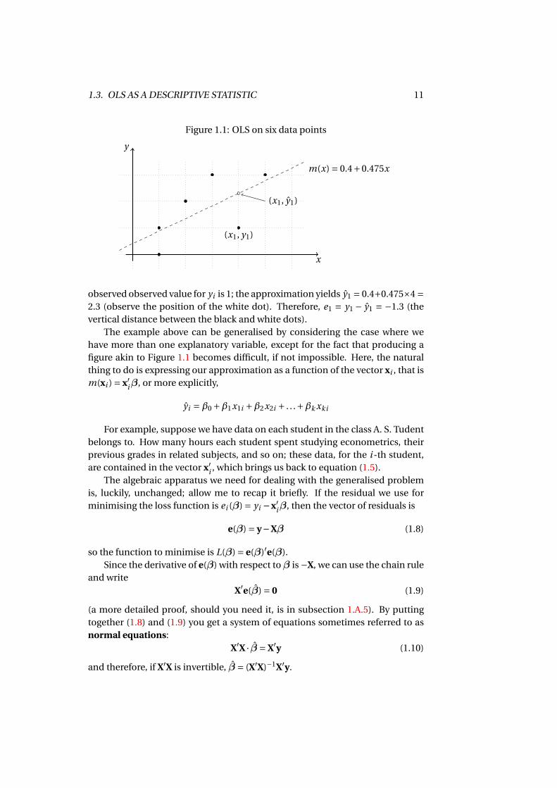
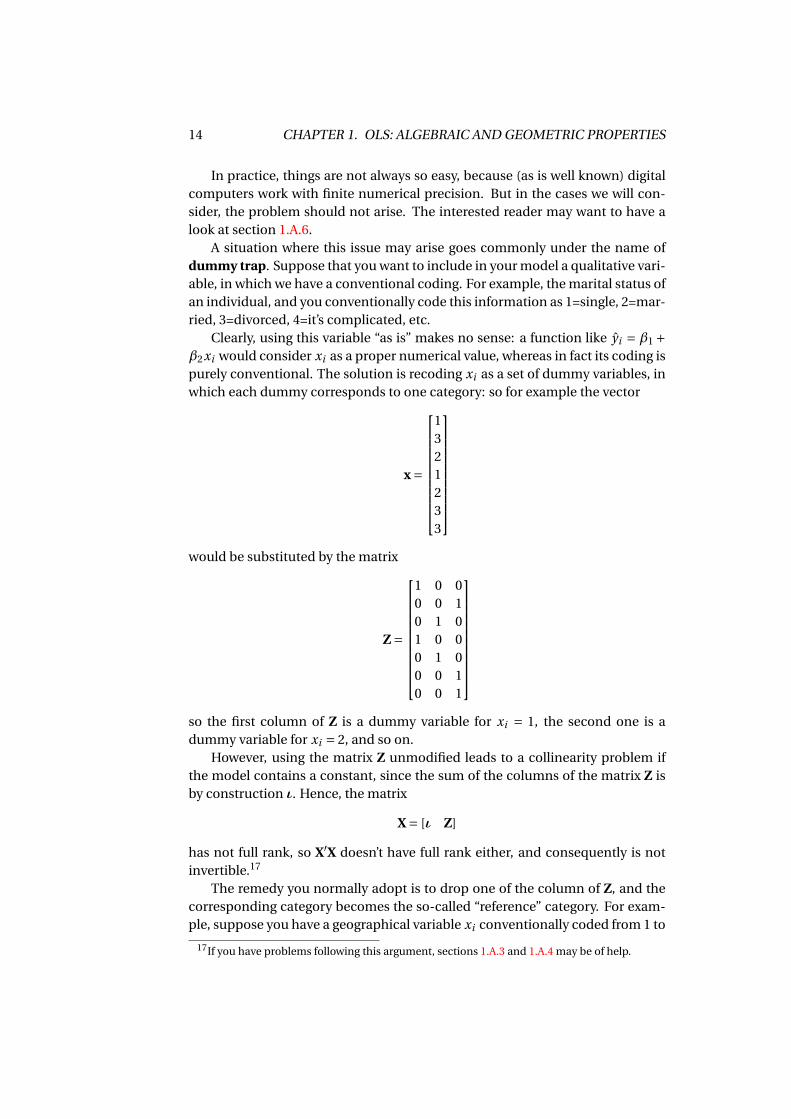
In traditional textbooks, at this point you always get a picture similar to theone in Figure 1.1, which is supposed to aid intuition; I don’t like it very much, andwill explain why shortly. Nevertheless, let me show it to you: in this example, weuse the same data as in the present example.
In Figure 1.1, each black dot corresponds to a (xi , yi ) pair; the dashed lineplots the m(x) function and the residuals are the vertical differences between thedots and the dashed line; the least squares criterion makes the line go throughthe dots in such a way that the sum of these differences (squared) is minimal.So, for example, for observation number 1 the observed value of xi is 4 and the
15Before you triumphantly shout “It’s wrong!”, remember to stick ι and x together.
1.3. OLS AS A DESCRIPTIVE STATISTIC 11
Figure 1.1: OLS on six data points
x
y
(x1, y1)
(x1, y1)
m(x) = 0.4+0.475x
observed observed value for yi is 1; the approximation yields y1 = 0.4+0.475×4 =2.3 (observe the position of the white dot). Therefore, e1 = y1 − y1 = −1.3 (thevertical distance between the black and white dots).
The example above can be generalised by considering the case where wehave more than one explanatory variable, except for the fact that producing afigure akin to Figure 1.1 becomes difficult, if not impossible. Here, the naturalthing to do is expressing our approximation as a function of the vector xi , that ism(xi ) = x′iβ, or more explicitly,
yi =β0 +β1x1i +β2x2i + . . .+βk xki
For example, suppose we have data on each student in the class A. S. Tudentbelongs to. How many hours each student spent studying econometrics, theirprevious grades in related subjects, and so on; these data, for the i -th student,are contained in the vector x′i , which brings us back to equation (1.5).
The algebraic apparatus we need for dealing with the generalised problemis, luckily, unchanged; allow me to recap it briefly. If the residual we use forminimising the loss function is ei (β) = yi −x′iβ, then the vector of residuals is
e(β) = y−Xβ (1.8)
so the function to minimise is L(β) = e(β)′e(β).Since the derivative of e(β) with respect toβ is −X, we can use the chain rule
and writeX′e(β) = 0 (1.9)
(a more detailed proof, should you need it, is in subsection 1.A.5). By puttingtogether (1.8) and (1.9) you get a system of equations sometimes referred to asnormal equations:
X′X · β = X′y (1.10)
and therefore, if X′X is invertible, β = (X′X)−1X′y.
12 CHAPTER 1. OLS: ALGEBRAIC AND GEOMETRIC PROPERTIES
CARL FRIEDRICH
GAUSS
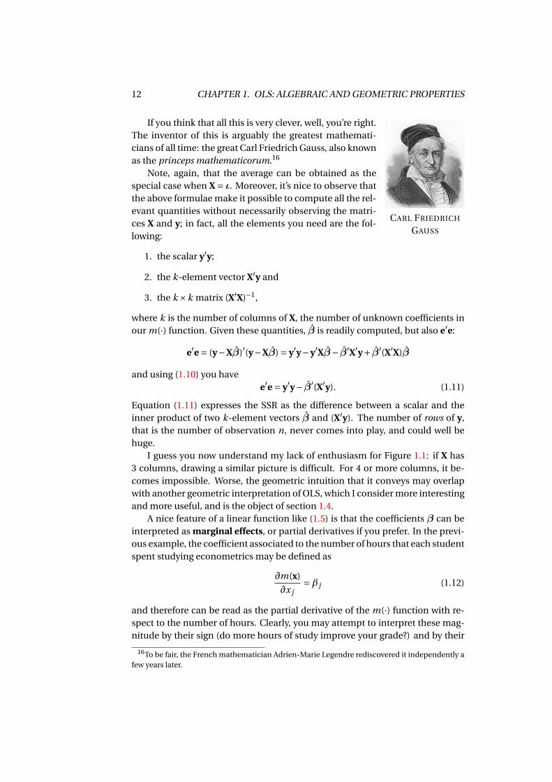
If you think that all this is very clever, well, you’re right.The inventor of this is arguably the greatest mathemati-cians of all time: the great Carl Friedrich Gauss, also knownas the princeps mathematicorum.16
Note, again, that the average can be obtained as thespecial case when X = ι. Moreover, it’s nice to observe thatthe above formulae make it possible to compute all the rel-evant quantities without necessarily observing the matri-ces X and y; in fact, all the elements you need are the fol-lowing:
1. the scalar y′y;
2. the k-element vector X′y and
3. the k ×k matrix (X′X)−1,
where k is the number of columns of X, the number of unknown coefficients inour m(·) function. Given these quantities, β is readily computed, but also e′e:
e′e = (y−Xβ)′(y−Xβ) = y′y−y′Xβ− β′X′y+ β′(X′X)β
and using (1.10) you havee′e = y′y− β′(X′y). (1.11)
Equation (1.11) expresses the SSR as the difference between a scalar and theinner product of two k-element vectors β and (X′y). The number of rows of y,that is the number of observation n, never comes into play, and could well behuge.
I guess you now understand my lack of enthusiasm for Figure 1.1: if X has3 columns, drawing a similar picture is difficult. For 4 or more columns, it be-comes impossible. Worse, the geometric intuition that it conveys may overlapwith another geometric interpretation of OLS, which I consider more interestingand more useful, and is the object of section 1.4.
A nice feature of a linear function like (1.5) is that the coefficients β can beinterpreted as marginal effects, or partial derivatives if you prefer. In the previ-ous example, the coefficient associated to the number of hours that each studentspent studying econometrics may be defined as
∂m(x)
∂x j=β j (1.12)
and therefore can be read as the partial derivative of the m(·) function with re-spect to the number of hours. Clearly, you may attempt to interpret these mag-nitude by their sign (do more hours of study improve your grade?) and by their
16To be fair, the French mathematician Adrien-Marie Legendre rediscovered it independently afew years later.
1.3. OLS AS A DESCRIPTIVE STATISTIC 13
magnitude (if so, by how much?). However, you should resist the temptation togive the coefficients a counterfactual interpretation (If A. S. Tudent had studied2 more hours, instead of watching that football game, by how much would theirmark have improved?); this is possible, in some circumstances, but not always(more on this in Section 3.5).
Focusing on marginal effects is what we domost often in econometrics, because the ques-tion of interest is not really approximating ygiven x, but rather understanding what the ef-fect of x on y is (and, possibly, how general androbust this effect is). In other words, the ob-ject of interest in econometrics is much moreoften β, rather than m(x). The opposite hap-pens in a broad class of statistical methods thatgo, collectively, by the name of machine learn-ing methods and focus much more on predic-tion than interpretation. In order to predict cor-rectly, these models use much more sophisti-cated ways of handling the data than a simplelinear function, and even writing the rule thatlinks x to y is impossible.Machine learning tools have been getting quite
popular at the beginning of the XXI century,and are the tools that companies like Googleand Amazon use to predict what video you’dlike to see on Youtube or what book you’d liketo buy when you open their website. As we allknow, these models perform surprisingly wellin practice, but nobody would be able to re-construct how their predictions come about.The phrase some people use is that machinelearning procedures are “black boxes”: theywork very well, but they don’t provide you withan explanation of why you like that particularvideo. The pros and cons of econometric mod-els versus machine learning tools are still un-der scrutiny by the scientific community, and,if you’re curious, I’ll just give you a pointer toMullainathan and Spiess (2017).
1.3.3 Collinearity and the dummy trap
Of course, for solving equation (1.10), X′X must be invertible. Now, you may ask:what if it’s singular? This is an interesting case. The solution y can still be found,but there is more than one vector β associated with it. In fact, there are infinitelymany. Let me give you an example. Suppose that X contain only one non-zerocolumn, x1. The solution is easy to find:
β1 =x′1y
x′1x1,
so that y = β1x1. Now, add to X a second column, x2, which happens to be amultiple of x1, so x2 = αx1. Evidently, x2 adds no information to our model,because it contains exactly the same information as x1 so y remains the same.Now, however, we can write it in infinitely may ways:
y =β1x1 = 0.5β1x1 +0.5β1
αx2 = 0.01β1x1 +0.99
β1
αx2 = . . .
because obviously β1
α x2 =β1x1. In other words, there are infinitely many ways tocombine x1 and x2 to obtain y, even though the latter is unique and the objectivefunction has a well-defined minimum.
We call this problem collinearity, or multicollinearity, and it can be solvedquite easily: all you have to do is drop the collinear columns until X has full rank.
14 CHAPTER 1. OLS: ALGEBRAIC AND GEOMETRIC PROPERTIES
In practice, things are not always so easy, because (as is well known) digitalcomputers work with finite numerical precision. But in the cases we will con-sider, the problem should not arise. The interested reader may want to have alook at section 1.A.6.
A situation where this issue may arise goes commonly under the name ofdummy trap. Suppose that you want to include in your model a qualitative vari-able, in which we have a conventional coding. For example, the marital status ofan individual, and you conventionally code this information as 1=single, 2=mar-ried, 3=divorced, 4=it’s complicated, etc.
Clearly, using this variable “as is” makes no sense: a function like yi = β1 +β2xi would consider xi as a proper numerical value, whereas in fact its coding ispurely conventional. The solution is recoding xi as a set of dummy variables, inwhich each dummy corresponds to one category: so for example the vector
x =
1321233
would be substituted by the matrix
Z =
1 0 00 0 10 1 01 0 00 1 00 0 10 0 1
so the first column of Z is a dummy variable for xi = 1, the second one is adummy variable for xi = 2, and so on.
However, using the matrix Z unmodified leads to a collinearity problem ifthe model contains a constant, since the sum of the columns of the matrix Z isby construction ι. Hence, the matrix
X = [ι Z]
has not full rank, so X′X doesn’t have full rank either, and consequently is notinvertible.17
The remedy you normally adopt is to drop one of the column of Z, and thecorresponding category becomes the so-called “reference” category. For exam-ple, suppose you have a geographical variable xi conventionally coded from 1 to
17If you have problems following this argument, sections 1.A.3 and 1.A.4 may be of help.
1.3. OLS AS A DESCRIPTIVE STATISTIC 15
3 (1=North, 2=Centre, 3=South). The model m(xi ) = β1 +β2xi is clearly mean-ingless, but one could think to set up an alternative model like
yi =β1 +β2Ni +β3Ci +β4Si ,
where Ni = 1 if the i -th observation pertains to the North, and so on. This wouldmake more sense, as all the variables in the model have a proper numerical in-terpretation. However, in this case we would have a collinearity problem.
The solution is dropping one of the geographical dummies from the model:for example, let’s say we drop the “South” dummy Si : the model would become
yi =β1 +β2Ni +β3Ci ;
observe that with the above formulation the fitted value for a southern observa-tion would be
yi =β1 +β2 ×0+β3 ×0 =β1
whereas for a northern one you would have
yi =β1 +β2 ×1+β3 ×0 =β1 +β2,
so β2 indicates the difference between a northern observation and a southernone, in the same way as β3 indicates the difference between Centre and South.More in general, after dropping one of the dummies, the coefficient for each ofthe remaining ones indicates the difference between that category and the oneyou chose as a reference.
1.3.4 Nonlinearity
A further step in enhancing this setup would be allowing for the possibility thatthe function m(xi ) is non-linear. In a traditional econometric setting this ideawould take us to consider the so-called NLS (Nonlinear Least Squares) tech-nique. I won’t go into this either, for two reasons.
First, because minimising a loss function like L(β) = ∑ni=1
[yi −m(xi ,β)
]2,where m(·) is some kind of crazy arbitrary function may be a difficult problem:it could have more than one solution, or none, or maybe one that cannot bewritten in closed form.
Second, the linear model is in fact more general than it seems, since in orderto use OLS it is sufficient that the model be linear in the parameters, not nec-essarily in the variables. For example, suppose that we have one explanatoryvariable; it is perfectly possible to use a model formulation like
m(xi ) =β1 +β2xi +β3x2i . (1.13)
The equation above contains a non-linear transformation of xi (the square), butthe function itself is just a linear combination of observable data: in this case,
16 CHAPTER 1. OLS: ALGEBRAIC AND GEOMETRIC PROPERTIES
we use a formulation that implies that the effect of xi on m(xi ) is nonlinear, butthis is still achieved by employing a linear combination of observable variables.To be more explicit, the X matrix would be, in this case,
X =
1 x1 x2
11 x2 x2
2...
1 xn x2n
and the algebra would proceed as usual.
This device is very common in applied econometrics, where powers of ob-servable variables are used to accommodate nonlinear effects in the model with-out having to give up the computational simplicity of OLS. The parameter β3 isalso quite easy to read: if it’s positive (negative), the m(xi ) function is convex(concave).
The only caveat we have to be aware of is that, of course, you cannot inter-pret the β vector as marginal effects, as the right-hand side of equation (1.12)is no longer a fixed scalar. In fact, the marginal effects for each variable in themodel become functions of the whole parameter vector β and of xi ; in otherterms, marginal effects may be different for each observation in our sample. Forexample, for the model in equation (1.13) the marginal effect of xi would be
∂m(xi )
∂xi=β2 +2β3xi ;
and its sign would depend on the condition xi > − β2
2β3, so it’s entirely possible
that the marginal effect of xi on yi is positive for some units in our sample andnegative for others.
More generally, what we can treat via OLS is the class of models where
m(xi ) =k∑
j=1β j g j (xi ),
where xi are our “base” explanatory variables and g j (·) is a sequence of arbitrarytransformations, no matter how crazy. Each element of this sequence becomesa column of the X matrix. Clearly, once you have computed the β vector, themarginal effects are easy to calculate:
∂m(xi )
∂xi=
k∑j=1
β j∂g j (xi )
∂xi.
1.4 The geometry of OLS
The OLS statistic and associated concepts can be given an interpretation thathas very little to do with statistics; instead, it’s a geometrical interpretation. Giventhe typical audience of this book, a few preliminaries may be in order here.
1.4. THE GEOMETRY OF OLS 17
The first concept we’ll want to define is the concept of distance (also knownas metric). Given two objects a and b, their distance is a function that shouldenjoy four properties:
1. d(a,b) = d(b, a)
2. d(a,b) ≥ 0
3. d(a,b) = 0 ⇔ a = b
4. d(a,b)+d(b,c) ≥ d(a,c)
The first three are obvious; as for the last one, called triangle inequality, it justmeans that the shortest way is the straight one. The objects in question may beof various sorts, but we will only consider the case when they are vectors. Thedistance of a vector from zero is its norm, written as ‖x‖ = d(x,0).
Many functions d(·) enjoy the four properties above, but the concept of dis-tance we use in everyday life is the so-called Euclidean distance, defined as
d(x,y) =√
(x−y)′(x−y)
and the reader may verify that the four properties are satisfied by this definition.Obviously, the formula for the Euclidean norm is ‖x‖ =p
x′x.The second concept I will use is the idea of a vector space. If you’re not
familiar with vector spaces, linear combinations and the rank of a matrix, thensections 1.A.2 and 1.A.3 are for you.
Consider the space Rn , where you have a vector y and a few vectors x j , withj = 1. . .k and k < n, all packed in a matrix X. What we want to find is the elementof Sp(X) which is closest to y. In formulae:
y = Argminx∈Sp(X)
‖y−x‖;
since the optimal point must belong to Sp(X), the problem can be rephrased as:find the vector β such that Xβ (that belongs to Sp(X) by construction) is closestto y:
β = Argminβ∈Rk
‖y−Xβ‖. (1.14)
If we decide to adopt the Euclidean definition of distance, then the solutionis exactly the same as the one to the statistical problem of Section 1.3.2: sincethe “square root” function is monotone, the minimum of ‖y−Xβ‖ is the same asthe minimum of (y−Xβ)′(y−Xβ), and therefore
Argminβ∈Rk
‖y−Xβ‖ = β = (X′X)−1X′y
from whichy = Xβ = X(X′X)−1X′y.
Note that y is a linear transform of y: you obtain y by premultiplying y by thematrix X(X′X)−1X′; this kind of transformation is called a “projection”.
18 CHAPTER 1. OLS: ALGEBRAIC AND GEOMETRIC PROPERTIES
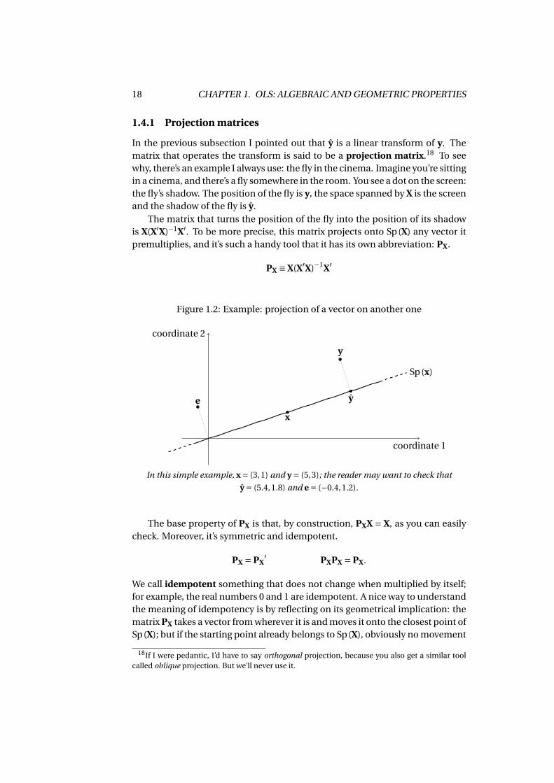
1.4.1 Projection matrices
In the previous subsection I pointed out that y is a linear transform of y. Thematrix that operates the transform is said to be a projection matrix.18 To seewhy, there’s an example I always use: the fly in the cinema. Imagine you’re sittingin a cinema, and there’s a fly somewhere in the room. You see a dot on the screen:the fly’s shadow. The position of the fly is y, the space spanned by X is the screenand the shadow of the fly is y.
The matrix that turns the position of the fly into the position of its shadowis X(X′X)−1X′. To be more precise, this matrix projects onto Sp(X) any vector itpremultiplies, and it’s such a handy tool that it has its own abbreviation: PX.
PX ≡ X(X′X)−1X′
Figure 1.2: Example: projection of a vector on another one
coordinate 1
coordinate 2
x
y
ye
Sp(x)
In this simple example, x = (3,1) and y = (5,3); the reader may want to check that
y = (5.4,1.8) and e = (−0.4,1.2).
The base property of PX is that, by construction, PXX = X, as you can easilycheck. Moreover, it’s symmetric and idempotent.
PX = PX′ PXPX = PX.
We call idempotent something that does not change when multiplied by itself;for example, the real numbers 0 and 1 are idempotent. A nice way to understandthe meaning of idempotency is by reflecting on its geometrical implication: thematrix PX takes a vector from wherever it is and moves it onto the closest point ofSp(X); but if the starting point already belongs to Sp(X), obviously no movement
18If I were pedantic, I’d have to say orthogonal projection, because you also get a similar toolcalled oblique projection. But we’ll never use it.
1.4. THE GEOMETRY OF OLS 19
takes place at all, so applying PX to a vector more than once produces no extraeffects (PXy = PXPXy = PXPX · · ·PXy).
It can also be proven that PX is singular;19 again, this algebraic property canbe given a nice intuitive geometric interpretation: a projection entails a lossof information, because some of the original coordinates get “squashed” ontoSp(X): in the fly example, it’s impossible to know the exact position of the flyfrom its shadow, because one of the coordinates (the distance from the screen)is lost. In formulae, the implication of PX being singular is that no matrix A existssuch that A·PX = I, and therefore no matrix exists such that Ay = y, which meansthat y is impossible to reconstruct from its projection.
In practice, when you regress y on X, you are performing exactly the samecalculations that are necessary to find the projection of y onto Sp(X), and thevector β contains the coordinates for locating y in that space.
There is another interesting matrix we’ll be using often:
MX = I−PX.
By definition, therefore, MXy = y− y = e. The MX matrix performs a complemen-tary task to that of PX: when you apply MX to a vector, it returns the differencebetween the original point and its projection. We may say that e = MXy containsthe information that is lost in the projection. It is easily checked that MXX = [0]and as a consequence,
MXPX = PXMX = [0],
where I’m using the notation [0] for “a matrix full of zeros”.Some more noteworthy properties: MX is symmetric, idempotent and sin-
gular, just like PX.20 As for is rank, it can be proven that its rank equals n − k,where n is the number of rows of X and r = rk(X).
A fundamental property this matrix enjoys is that every vector of the typeMXy is orthogonal to Sp(X), so it forms a 90° angle with any vector that can bewritten as Xλ.21 These properties are very convenient in many cases; a notableone is the possibility of rewriting the SSR as a quadratic form:22.
e′e = (MXy)′(MXy) = y′MXMXy = y′MXy
where the second equality comes from symmetry and the third one from idem-potency. By the way, the above expression could be further manipulated to re-
19To be specific: it can be proven that rk(PX) = rk(X), so PX is a n ×n matrix with rank k; evi-dently, in the situation we’re considering here, n > k. Actually, it can be proven that no idempotentmatrix is invertible, the identity matrix being the only exception.
20In fact, MX is itself a projection matrix, but let’s not get into this, ok?21Let me remind the reader that two vectors are said to be orthogonal if their inner product is
0. In formulae: x ⊥ y ⇔ x′y = 0. A vector is orthogonal to a space if it’s orthogonal to all the pointsthat belong to that space: y ⊥ Sp(X) ⇔ y′X = 0, so y ⊥ Xλ for any λ.
22A quadratic form is an expression like x′Ax, where x is a vector and A is a square matrix,usually symmetric. I sometimes use the metaphor of a sandwich and call x the “bread” and A the“cheese”.
20 CHAPTER 1. OLS: ALGEBRAIC AND GEOMETRIC PROPERTIES
obtain equation (1.11):
y′MXy = y′(I−PX)y = y′y−y′PXy = y′y−y′X(X′X)−1X′y = y′y− β′(X′y).
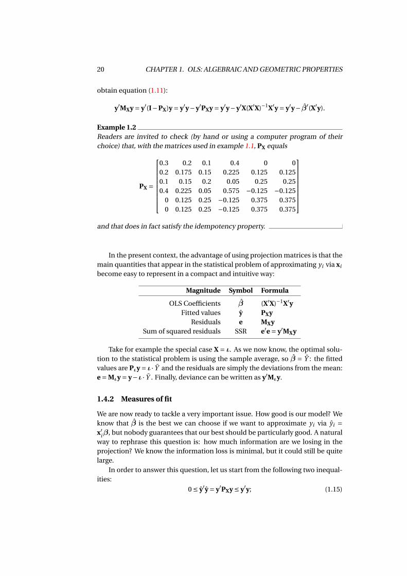
Example 1.2Readers are invited to check (by hand or using a computer program of theirchoice) that, with the matrices used in example 1.1, PX equals
PX =
0.3 0.2 0.1 0.4 0 00.2 0.175 0.15 0.225 0.125 0.1250.1 0.15 0.2 0.05 0.25 0.250.4 0.225 0.05 0.575 −0.125 −0.125
0 0.125 0.25 −0.125 0.375 0.3750 0.125 0.25 −0.125 0.375 0.375
and that does in fact satisfy the idempotency property.
In the present context, the advantage of using projection matrices is that themain quantities that appear in the statistical problem of approximating yi via xi
become easy to represent in a compact and intuitive way:
Magnitude Symbol Formula
OLS Coefficients β (X′X)−1X′yFitted values y PXy
Residuals e MXySum of squared residuals SSR e′e = y′MXy
Take for example the special case X = ι. As we now know, the optimal solu-tion to the statistical problem is using the sample average, so β = Y : the fittedvalues are Pιy = ι · Y and the residuals are simply the deviations from the mean:e = Mιy = y−ι · Y . Finally, deviance can be written as y′Mιy.
1.4.2 Measures of fit
We are now ready to tackle a very important issue. How good is our model? Weknow that β is the best we can choose if we want to approximate yi via yi =x′iβ, but nobody guarantees that our best should be particularly good. A naturalway to rephrase this question is: how much information are we losing in theprojection? We know the information loss is minimal, but it could still be quitelarge.
In order to answer this question, let us start from the following two inequal-ities:
0 ≤ y′y = y′PXy ≤ y′y; (1.15)
1.4. THE GEOMETRY OF OLS 21
the first one is rather obvious, considering that y′y is a sum of squares, andtherefore non-negative. The other one, instead, can be motivated via y′PXy =y′y−y′MXy = y′y−e′e; since e′e is also a sum of squares, y′PXy ≤ y′y. If we divideeverything by y′y, we get
0 ≤ y′yy′y
= 1− e′ey′y
= R2u ≤ 1. (1.16)
This index bears the name R2u (“uncentred R-squared”), and, as the above
expression shows, it’s bounded by construction between 0 and 1. It can be givena very intuitive geometric interpretation: evidently, in Rn the points 0, y and yform a right triangle (see also Figure 1.2), in which you get a “good” leg, that is y,and a “bad” one, the segment linking y and y, which is congruent to e: we’d likethe bad leg to be as short as possible. After Pythagoras’ theorem, the R2
u indexgives us (the square of) the ratio between the good leg and the hypotenuse. Ofcourse, we’d like this ratio to be as close to 1 as possible.
Example 1.3With the matrices used in example 1.1, you get that y′y = 29 and e′e = 1.5; there-fore,
R2u = 1− 1.5
29' 0.9483
The R2u index makes perfect sense geometrically, but hardly any from a sta-
tistical point of view: the quantity y′y has a natural geometrical interpretation,but statistically it doesn’t mean much, unless we give it the meaning
y′y = (y−0)′(y−0),
that is, the SSR for a model in which y = 0. Such a model would be absolutelyminimal, but rather silly as a model. Instead, we might want to use as a bench-mark our initial proposal described in section 1.2, where X = ι. In this case,the SSR is just the deviance of y, that is the sum of squared deviations from themean, which can be written as y′Mιy. If ι ∈ Sp(X) (typically, when the modelcontains a constant term), then a decomposition similar to (1.15) is possible:since y = y+e, then obviously
y′Mιy = y′Mιy+e′Mιe = y′Mιy+e′e (1.17)
because if ι ∈ Sp(X), then Mιe = e.23 Therefore,
0 ≤ e′e ≤ y′Mιy,
23Subsection 1.A.8 should help the readers who want this result proven.
22 CHAPTER 1. OLS: ALGEBRAIC AND GEOMETRIC PROPERTIES
where the second inequality comes from the fact that y′Mιy is a sum of squaresand therefore non-negative. The modified version of R2 is known as centredR-square:
R2 = 1− e′ey′Mιy
. (1.18)
The concept of R2 that we normally use in econometrics is the centred one, andthis is why the index defined at equation (1.16) has the “u” as a footer (from theword uncentred).
In a way, the definition of R2 is implicitly based on a comparison betweendifferent models: one which uses all the information contained in X and another(smaller) one, which only uses ι, because y′Mιy is just the SSR of a model inwhich we regress y on ι. Therefore, equation (1.18) can be read as a way to com-pare the loss function for those two models.
In fact, this same idea can be pushed a little bit further: imagine that wewanted to compare model A and model B, in which B contains the same ex-planatory variables as A, plus some more. In practice:
Model A y ' Xβ
Model B y ' Xβ+Zγ = Wθ
where W = [X Z] and θ =[βγ
].
The matrix Z contains additional regressors to model A. It is important torealise that the information contained in Z could be perfectly relevant and le-gitimate, but also ridiculously useless. For example, a model for the academicperformance of A. S. Tudent could well contain, as an explanatory variable, thenumber of pets A. S. Tudent’s neighbours have, or the distance between A. S. Tu-dent’s bed and St. Peter’s basilica in Rome.
It’s easy to prove that the SSR for model B is always smaller than that for A:
SSRA = e′aea SSRB = e′beb
where ea = MXy and eb = MWy. Since X ∈ Sp(W), clearly PWX = X and therefore
MWMX = MW,
which implies MWea = eb ; as a consequence,
SSRB = e′beb = e′aMWea = e′aea −e′aPWea ≤ e′aea = SSRA .
More generally, if Sp(W) ⊃ Sp(X), then y′MWy ≤ y′MXy for any vector y.The implication is: if we had to choose between A and B by using the SSR
as a criterion, model B would always be the winner, no matter how absurd thechoice of the variables Z is. The R2 index isn’t any better: proving that
SSRB ≤ SSRA ⇒ R2B ≥ R2
A .
1.5. THE FRISCH-WAUGH THEOREM 23
is a trivial exercise, so if you add any explanatory variable to an existing model,the R2 index cannot become smaller.
A possible solution could be using a slight variation of the index, which goesby the name of adjusted R2:
R2 = 1− e′e
y′Mιy
n −1
n −k, (1.19)
where n is the size of our dataset and k is the number of explanatory variables. Itis easy to prove that if you add silly variables to a model, so that the SSR changesonly slightly, the n − k in the denominator should offset that effect. However,as we will see in section 3.3.2, the best way of choosing between models is byframing the decision in a proper inferential context.
1.5 The Frisch-Waugh theorem
Projection matrices are also useful to illustrate a remarkable result, known as theFrisch-Waugh theorem:24 given a model of the kind y = Xβ+e, split X verticallyinto two sub-matrices Z and W, and β accordingly
y = [Z W
][β1
β2
]Applying equation (1.7) we get the following:[
β1
β2
]=
[Z′Z Z′WW′Z W′W
]−1 [Z′yW′y
]It would seem that finding an analytical closed form for β1 and β2 as func-
tions of Z, W and y is quite difficult; fortunately, it isn’t so: start from
y = y+e = Zβ1 +Wβ2 +e
and premultiply the equation above by MW:
MWy = MWZβ1 +e,
since MWW = 0 (by construction) and MWe = e (because e = MXy, but Sp(W) ⊂Sp(X), so MWMX = MX).25 Now premultiply by Z′:
Z′MWy = Z′MWZβ1
since Z′e = 0. As a consequence,
24In fact, many call this theorem the Frisch-Waugh-Lovell theorem, as it was Micheal Lovellwho, in a paper appeared in 1963, generalised the original result that Frisch and Waugh had ob-tained 30 years earlier to its present form.
25If you’re getting a bit confused, you may want to take a look at section 1.A.8.
24 CHAPTER 1. OLS: ALGEBRAIC AND GEOMETRIC PROPERTIES
β1 =(Z′MWZ
)−1 Z′MWy (1.20)
Since MW is idempotent, an alternative way to write (1.20) could be
β1 =[(Z′MW)(MWZ)
]−1 (Z′MW)(MWy);
therefore β1 is the vector of the coefficients for a model in which the dependentvariable is the vector of the residuals of y with respect to W and the regressormatrix is the matrix of residuals of Z with respect to W. For symmetry reasons,you also obviously get a corresponding expression for β2:
β2 =(W′MZW
)−1 W′MZy
In practice, a perfectly valid algorithm for computing β1 could be:
1. regress y on W; take the residuals and call them y;
2. regress each column of Z on W; form a matrix with the residuals and call itZ;
3. regress y on Z: the result is β1.
This result is not just a mathematical curiosity, nor a computational gim-mick: it comes in handy in a variety of situations for proving theoretical results.For example, consider the case when X can be written as
X = [Z u],
where u is a column vector containing all zeros except for the m-th element,which is 1.26
In scalar form, our model would read
yi = z′iβ+uiγ+ei
where is a dummy variable such that ui = 1 if i = m and 0 otherwise. Thanks tothe Frisch-Waugh theorem, it’s easy to prove that the OLS coefficient for Z canbe written as
β =[ ∑
i 6=mzi z′i
]−1 ∑i 6=m
zi yi ; (1.21)
that is, the coefficient you would get if you regressed y on Z alone on a sam-ple that contains all observations except for the m-th one. The proof, if you’reinterested, is in section 1.A.9.
26Some call a vector like u a basis vector. Others simply say “the m-th column of the identitymatrix”. We’ll re-use this concept in section 3.3.1 and call u an “extraction vector”.
1.6. AN EXAMPLE 25
An interpretation that this theorem can be given is the following: the coef-ficients for a group of regressors measure the response of y having taken intoaccount the other ones or, as we say, “everything else being equal”. The phrasenormally used in the profession is “controlling for”. For example: suppose that ycontains data on the wages for n employees, that Z is their education level andW is a geographical dummy variable (North vs South). The vector y = MWy willcontain the differences between the individual wages and the average wage ofthe region where they live, in the same way as Z = MWZ contains the data oneducation as deviation from the regional mean. Therefore, regressing y on Z isa way to implicitly take into account that differences in wages between regionsmay depend on different educational levels. Consequently, by regressing y onboth the “education” variable and the regional dummy variable, the coefficientfor education will measure its effect on wages controlling for geographical ef-fects.
1.6 An example
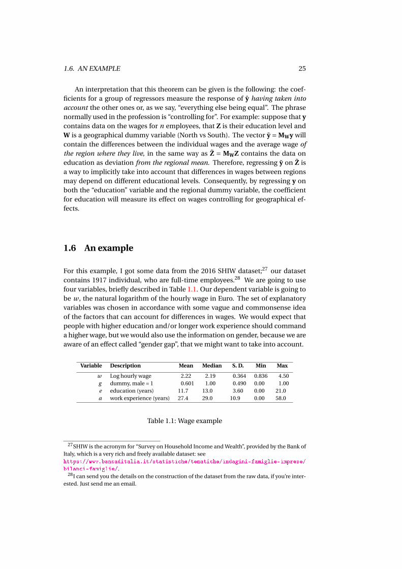
For this example, I got some data from the 2016 SHIW dataset;27 our datasetcontains 1917 individual, who are full-time employees.28 We are going to usefour variables, briefly described in Table 1.1. Our dependent variable is going tobe w , the natural logarithm of the hourly wage in Euro. The set of explanatoryvariables was chosen in accordance with some vague and commonsense ideaof the factors that can account for differences in wages. We would expect thatpeople with higher education and/or longer work experience should commanda higher wage, but we would also use the information on gender, because we areaware of an effect called “gender gap”, that we might want to take into account.
Variable Description Mean Median S. D. Min Max
w Log hourly wage 2.22 2.19 0.364 0.836 4.50g dummy, male = 1 0.601 1.00 0.490 0.00 1.00e education (years) 11.7 13.0 3.60 0.00 21.0a work experience (years) 27.4 29.0 10.9 0.00 58.0
Table 1.1: Wage example
27SHIW is the acronym for “Survey on Household Income and Wealth”, provided by the Bank ofItaly, which is a very rich and freely available dataset: seehttps://www.bancaditalia.it/statistiche/tematiche/indagini-famiglie-imprese/
bilanci-famiglie/.28I can send you the details on the construction of the dataset from the raw data, if you’re inter-
ested. Just send me an email.
26 CHAPTER 1. OLS: ALGEBRAIC AND GEOMETRIC PROPERTIES
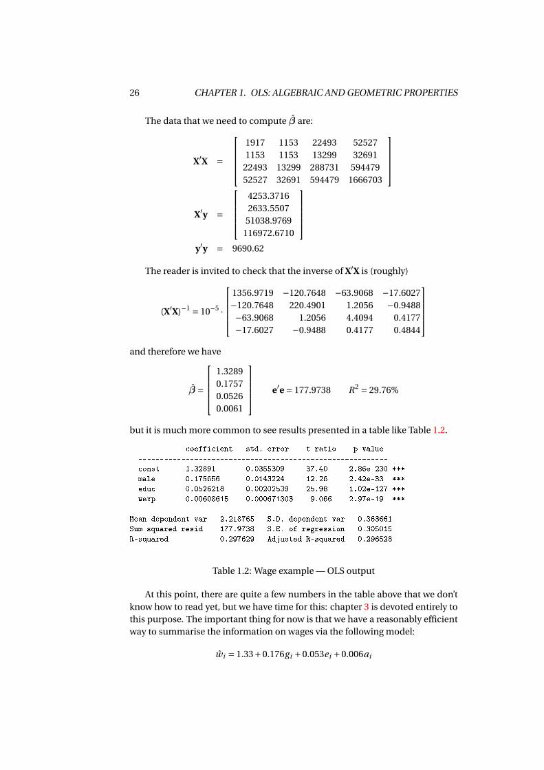
The data that we need to compute β are:
X′X =
1917 1153 22493 525271153 1153 13299 32691
22493 13299 288731 59447952527 32691 594479 1666703
X′y =
4253.37162633.5507
51038.9769116972.6710
y′y = 9690.62
The reader is invited to check that the inverse of X′X is (roughly)
(X′X)−1 = 10−5 ·
1356.9719 −120.7648 −63.9068 −17.6027−120.7648 220.4901 1.2056 −0.9488−63.9068 1.2056 4.4094 0.4177−17.6027 −0.9488 0.4177 0.4844
and therefore we have
β =
1.32890.17570.05260.0061
e′e = 177.9738 R2 = 29.76%
but it is much more common to see results presented in a table like Table 1.2.
coefficient std. error t-ratio p-value
----------------------------------------------------------
const 1.32891 0.0355309 37.40 2.86e-230 ***
male 0.175656 0.0143224 12.26 2.42e-33 ***
educ 0.0526218 0.00202539 25.98 1.02e-127 ***
wexp 0.00608615 0.000671303 9.066 2.97e-19 ***
Mean dependent var 2.218765 S.D. dependent var 0.363661
Sum squared resid 177.9738 S.E. of regression 0.305015
R-squared 0.297629 Adjusted R-squared 0.296528
Table 1.2: Wage example — OLS output
At this point, there are quite a few numbers in the table above that we don’tknow how to read yet, but we have time for this: chapter 3 is devoted entirely tothis purpose. The important thing for now is that we have a reasonably efficientway to summarise the information on wages via the following model:
wi = 1.33+0.176gi +0.053ei +0.006ai
1.A. ASSORTED RESULTS 27
where wi is the log wage for individual i , gi is their gender, and the rest follows.The approximation is not bad: the R2 index is roughly 30%, which means that ifwe compare the loss functions for our model and the one we get if we has justused the average wage, we get
0.298 = 1− e′ey′Mιy
=⇒ e′e = 0.702 ·y′Mιy;
not bad at all.
In practice, if we had a guy who studied for 13 years and has worked for 20years, we would guess that the log of his hourly wage would be
1.33+0.176 ·1+0.052 ·13+0.006 ·20 ' 2.31
which is roughly €10 an hour (which sounds reasonable).
Of course, nothing is stopping us from interpreting the sign and magnitudeof our OLS coefficients: for example, the coefficient for education is about 5%,and therefore the best way to use the educational attainment variable for sum-marising the data we have on wages is by saying that each year of extra edu-cation gives you a guess which is about 5% higher.29 Does this imply that youget positive returns to education in the Italian labour market? Strictly speaking,it doesn’t. This number yields a fairly decent approximation to our dataset of1917 people. To assume that the same regularity should hold for others is totallyunwarranted. And the same goes for the gender gap: it would seem that beingmale shifts your fitted wage by 17.5%. But again, at the risk of being pedantic,all we can say is that among our 1917 data points, males get (on average) moremoney than females with the same level of experience and education. Coinci-dence? We should be wary of generalisations, however tempting they may be toour sociologist self.
And yet, these thoughts are perfectly natural. The key ingredient to give sci-entific legitimacy to this sort of mental process is to frame it in the context ofstatistical inference, which is the object of the next chapter.
1.A Assorted results
This section contains several results on matrix algebra, in the simplest form pos-sible. If you want an authoritative reference, my advice is to get a copy of Hornand Johnson (2012) or Lütkepohl (1996).
29One of the reasons why we economists love logarithms is that they auto-magically turn abso-
lute changes into relative ones: β2 = dwde = dln(W )
de = 1W
dWde ' ∆W /W
∆e . In other words, the coeffi-cient associated with the educational variable gives you a measure of the relative change in wagein response to a unit increase in education.
28 CHAPTER 1. OLS: ALGEBRAIC AND GEOMETRIC PROPERTIES
1.A.1 Matrix differentiation rules
The familiar concept of a derivative of a function of a scalar can be generalisedto functions of a vector
y = f (x),
where you have a real number y for every possible vector x. For example, ify = x + w z , you can define the vector x = [x, w, z]′. The generalisation of theconcept of derivative is what we call the gradient, that is a vector collecting thepartial derivatives with respect to the corresponding elements of x. We adopt theconvention by which the gradient is a row vector; hence, for the example above,the gradient is
∂y
∂x=
[∂y∂x
∂y∂w
∂y∂z
]= [
1 zw z−1 log(w) ·w z]
The cases we’ll need are very simple, because they generalise the simple uni-variate functions y = ax and y = ax2. Let’s begin by
f (x) = a′x =n∑
i=1ai xi ;
evidently, the partial derivative of f (x) with respect to xi is just ai ; by stacking allthe partial derivatives into a vector, the result is just the vector a, and therefore
d
dxa′x = a′
note that the familiar rule ddx ax = a is just a special case when a and x are
scalars.As for the quadratic form
f (x) = x′Ax =n∑
i=1
n∑j=1
ai j xi x j ;
it can be proven easily (but it’s rather boring) that
d
dxx′Ax = x′(A+ A′)
and of course if A is symmetric (as in most cases), then ddx x′Ax = 2 ·x′A. Again,
note that the scalar case ddx ax2 = 2ax is easy to spot as a special case.
One last thing: the convention by which differentiation expands “by row”turns out to be very useful because it makes the chain rule for the derivatives“just work” automatically. For example, suppose you have y = Ax and z = By;of course, if you need the derivative of z with respect to x you may proceed bydefining C = B · A and observing that
z = B (Ax) =C x =⇒ ∂z
∂x=C
but you may also get the same result via the chain rule, as
∂z
∂x= ∂z
∂y
∂y
∂x= B · A =C .
1.A. ASSORTED RESULTS 29
1.A.2 Vector spaces
Here we will draw heavily on the fact that a vector with n elements can be thoughtof as a point in an n-dimensional space: a scalar is a point on the real line, a vec-tor with two elements is a point on a plane, and so on. Actually, the notationx ∈Rn is a concise way of saying that x has n elements.
There are two basic operations we can perform on vectors: (i) multiplying avector by a scalar and (ii) summing two vectors. In both cases, the result you getis another vector. Therefore, if you consider k vectors with n elements each, itmakes sense to define an operation called a linear combination of them:
z =λ1x1 +λ2x2 +·· ·+λk xk =k∑
j=1λ j x j ;
note that the above could have been written more compactly in matrix notationas z = Xλ, where X is a matrix whose columns are the vectors x j and λ is a k-element vector.
The result is, of course, an n-element vector, that is a point in Rn . But thek vectors x1, . . . ,xk are also a cloud of k points in Rn ; so we may ask ourselves ifthere is any kind of geometrical relationship between z and x1,x2, . . . ,xk .
Begin by considering the special case k = 1. Here z is just a multiple of x1;longer, if |λ1| > 1, shorter otherwise; mirrored across the origin if λ1 < 0, in thesame quadrant otherwise. Easy, boring. Note that, if you consider the set of allthe vectors z you can obtain by all possible choices for λ1, you get a straight linegoing through the origin, and of course x1; this set of points is called the spacespanned, or generated by x1; or, in symbols, Sp(x1). It’s important to note thatthis won’t work if x1 = 0: in this case, Sp(x1) is not a straight line, but rather apoint (the origin).
If you have two vectors, instead, the standard case occurs when they are notaligned with respect to the origin. In this case, Sp(x1,x2) is a plane and z =λ1x1+λ2x2 is a point somewhere on that plane. Its exact location depends on λ1 andλ2, but note that
• by a suitable choice of λ1 and λ2, no point on the plane is unreachable;
• no matter how you choose λ1 and λ2, you can’t end up outside the plane.
However, if x2 is a multiple of x1, then x2 ∈ Sp(x1) and Sp(x1,x2) = Sp(x1), that isa line, and not a plane. In this case, considering x2 won’t make Sp(x1) “grow” indimension, since x2 is already contained in it, so to speak.
In order to fully generalise the point, we use the concept of linear indepen-dence: a set of k vectors x1, . . . ,xk is said to be linearly independent if none ofthem can be expressed as a linear combination of the remaining ones.30 The
30The usual definition is that x1, . . . ,xk are linearly independent if no linear combination∑kj=1λ j x j is zero unless all the λ j are zero. The reader is invited to check that the two defini-
tions are equivalent.
30 CHAPTER 1. OLS: ALGEBRAIC AND GEOMETRIC PROPERTIES
case I called “standard” a few lines above happens when x1 and x2 are linearlyindependent.
1.A.3 Rank of a matrix
If we take k vectors with n elements each and we arrange them side by side so asto form an (n ×k) matrix (call it X), the maximum number of linearly indepen-dent columns of X is the rank of X (rk(X) in formulae). The rank function enjoysseveral nice properties:
1. 0 ≤ rk(X) ≤ k (by definition)
2. rk(X) = rk(X′) (I’m not proving this for the sake of brevity)
3. 0 ≤ rk(X) ≤ min(k,n) (by putting together the previous two); but if rk(X) =min(k,n), and the rank hits its maximal value, the matrix is said to have“full rank”
4. rk(A ·B) ≤ min(rk(A) , rk(B)); but in the special case when A′ = B , thenequality holds, and rk
(B ′B
)= rk(BB ′)= rk(B)
We can use the rank function to measure the dimension of the space spannedby X. For example, if rk(X) = 1, then Sp(X) is a line, if rk(X) = 2, then Sp(X) is aplane, and so on. This number may be smaller than the number of columns ofX.
A result we will not use very much (only in chapter 6), but is quite useful toknow in more advanced settings is that, if you have a matrix A with n rows, kcolumns and rank r , it is always possible to write it as
A =UV ′
where U is (n × r ), V is (k × r ), and both have rank r . For any non-zero A, thereare infinitely many pairs of matrices that satisfy the decomposition above. Forexample, the matrix
A =1 0
0 00 0
can be written as
A =1
00
[1 0
]as well as
A =−10
00
[−0.1 0]
1.A. ASSORTED RESULTS 31
1.A.4 Rank and inversion
A square matrix A is said to be “invertible” if there is another matrix B such thatAB = B A = I , where I is the identity matrix. if B exists, it’s also notated as A−1
and called the inverse of A; otherwise, A is said to be singular.
The mathematically accepted way to say “A is non-singular” is by writing|A| 6= 0, where the symbol |A| is used for the determinant of the matrix A, whichis a scalar function such that |A| = 0 if and only if A is singular.31
The concept of matrix inversion becomes quite intuitive if you look at it ge-ometrically. Take a vector x with n elements. If you pre-multiply it by a squarematrix A you get another vector with n elements:
y = A x;
in practice, A defines a displacement that takes you from a point in Rn to a pointin the same space. Is it possible to “undo” this movement? If A takes you fromx to y, is there a matrix B that performs the return trip? If such a matrix exists,then
x = B y.
The only way to guarantee that this happens for every pair of vectors x and y isto have
AB = B A = I .
Now, note that y is a linear combination of the columns of A; intuition sug-gests that all the n separate pieces of information originally contained in x canget preserved during the trip only if the rank of A is n. In fact, it can be provenformally that if A is an (n ×n) matrix, then rk(A) = n is a necessary and suffi-cient condition for A−1 to exist: for square matrices, full rank is the same thingas invertibility.
The world of matrix algebra is populated withresults that appear unintuitive when you’reused to the algebra of scalars. A notable oneis: any matrix A (even singular ones; evennon-square ones) admits a matrix B such thatAB A = A and B AB = B ; B is called the “Moore-
Penrose” pseudo-inverse. For example, the ma-
trix A =[
1 00 0
]is singular, and therefore has
no inverse. However, it’s got a pseudo-inverse,which is A itself. In fact, all projection matricesare their own pseudo-inverses.
Computing an inverse in practice is very boring: this is one of those tasksthat computers are very good at, while humans are not. The only interestingcases for which I’m giving you instructions on how to invert a matrix by handare:
31You almost never need to compute a determinant by hand, so I’ll spare you its definition. Ifyou’re curious, there’s always Wikipedia.
32 CHAPTER 1. OLS: ALGEBRAIC AND GEOMETRIC PROPERTIES
1. when A is 2×2. In this case, it’s easy to memorise the explicit formula forthe inverse: (
a bc d
)−1
= 1
ad −bc
(d −b
−c a
);
2. when A is block-diagonal, that is it can be written as
A =
A1 0 · · · 00 A2 · · · 0...
.... . .
...0 0 . . . Am
;
if the inverse exists, it has the same structure:
A−1 =
A−1
1 0 · · · 00 A−1
2 · · · 0...
.... . .
...0 0 . . . A−1
m
.
There are many nice properties that invertible matrices enjoy. For example:
• the inverse, if it exists, is unique; that is, if AB = I = AC , then B =C ;
• the inverse of a symmetric matrix is also symmetric;
• the transpose of the inverse is the inverse of the transpose ((A′)−1 = (A−1)′);
• if a matrix is positive definite (see next section), then its inverse is positivedefinite too;
• if A is invertible, then the only solution to Ax = 0 is x = 0; conversely, if Ais singular, then there exists at least one non-zero vector such that Ax = 0.
• if A and B are invertible, then (AB)−1 = B−1 A−1.
1.A.5 Step-by-step derivation of the sum of squares function
The function we have to differentiate with respect to β is
L(β) = e(β)′e(β);
the elegant way to do this is by using the chain rule:
∂L(β)
∂β= ∂e(β)
∂β
′e(β)+
[e(β)′
∂e(β)
∂β
]′= 2 · ∂e(β)
∂β
′e(β);
the reason why we have to transpose the second element of the sum in the equa-tion above is conformability: you can’t sum a row vector and a column vector.
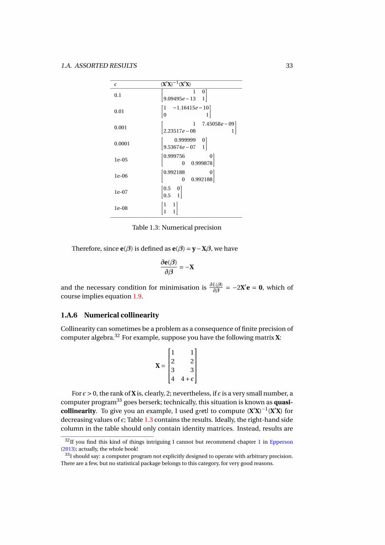
1.A. ASSORTED RESULTS 33
ε (X′X)−1(X′X)
0.1
[1 0
9.09495e −13 1
]0.01
[1 −1.16415e −100 1
]0.001
[1 7.45058e −09
2.23517e −08 1
]0.0001
[0.999999 0
9.53674e −07 1
]1e-05
[0.999756 0
0 0.999878
]1e-06
[0.992188 0
0 0.992188
]1e-07
[0.5 00.5 1
]1e-08
[1 11 1
]
Table 1.3: Numerical precision
Therefore, since e(β) is defined as e(β) = y−Xβ, we have
∂e(β)
∂β=−X
and the necessary condition for minimisation is ∂L(β)∂β = −2X′e = 0, which of
course implies equation 1.9.
1.A.6 Numerical collinearity
Collinearity can sometimes be a problem as a consequence of finite precision ofcomputer algebra.32 For example, suppose you have the following matrix X:
X =
1 12 23 34 4+ε
For ε> 0, the rank of X is, clearly, 2; nevertheless, if ε is a very small number, a
computer program33 goes berserk; technically, this situation is known as quasi-collinearity. To give you an example, I used gretl to compute (X′X)−1(X′X) fordecreasing values of ε; Table 1.3 contains the results. Ideally, the right-hand sidecolumn in the table should only contain identity matrices. Instead, results are
32If you find this kind of things intriguing I cannot but recommend chapter 1 in Epperson(2013); actually, the whole book!
33I should say: a computer program not explicitly designed to operate with arbitrary precision.There are a few, but no statistical package belongs to this category, for very good reasons.
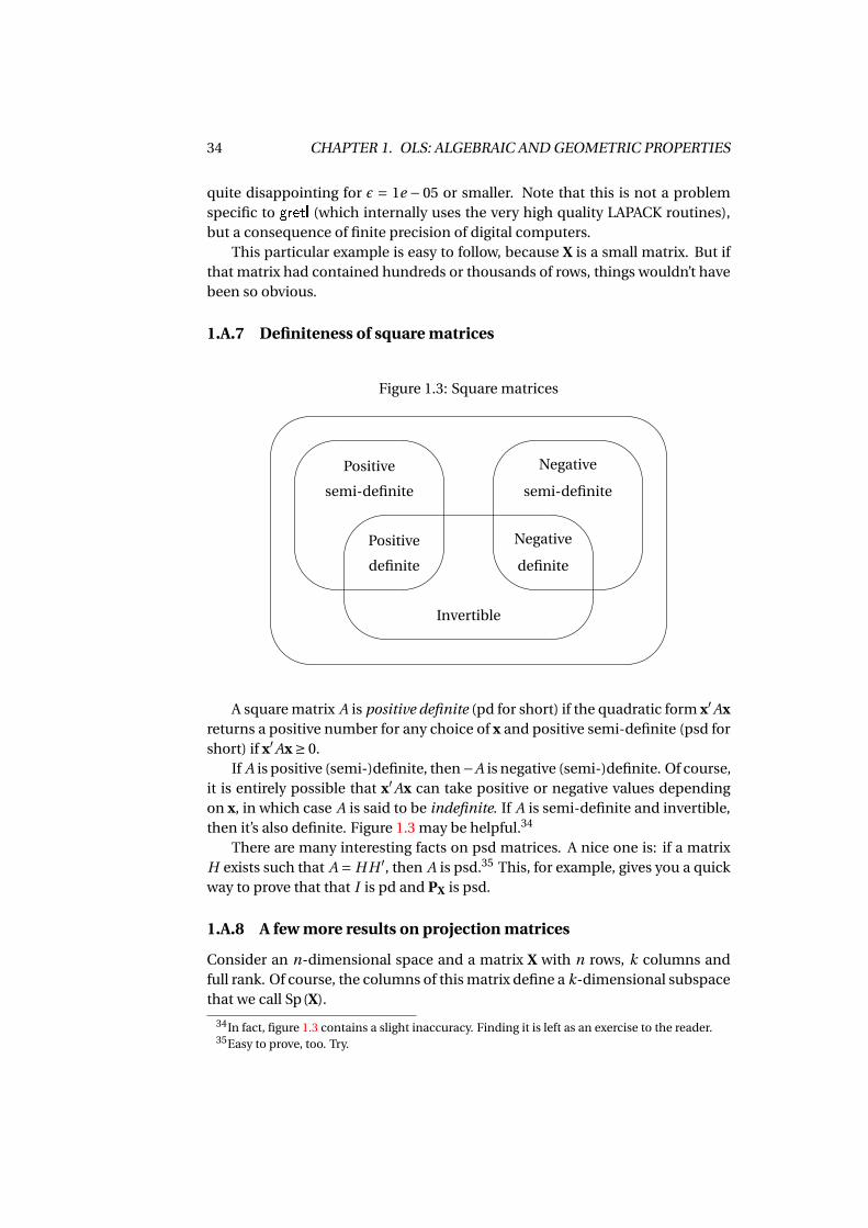
34 CHAPTER 1. OLS: ALGEBRAIC AND GEOMETRIC PROPERTIES
quite disappointing for ε = 1e − 05 or smaller. Note that this is not a problemspecific to gretl (which internally uses the very high quality LAPACK routines),but a consequence of finite precision of digital computers.
This particular example is easy to follow, because X is a small matrix. But ifthat matrix had contained hundreds or thousands of rows, things wouldn’t havebeen so obvious.
1.A.7 Definiteness of square matrices
Figure 1.3: Square matrices
Invertible
Positive
semi-definite
Negative
semi-definite
Positive
definite
Negative
definite
A square matrix A is positive definite (pd for short) if the quadratic form x′Axreturns a positive number for any choice of x and positive semi-definite (psd forshort) if x′Ax ≥ 0.
If A is positive (semi-)definite, then−A is negative (semi-)definite. Of course,it is entirely possible that x′Ax can take positive or negative values dependingon x, in which case A is said to be indefinite. If A is semi-definite and invertible,then it’s also definite. Figure 1.3 may be helpful.34
There are many interesting facts on psd matrices. A nice one is: if a matrixH exists such that A = H H ′, then A is psd.35 This, for example, gives you a quickway to prove that that I is pd and PX is psd.
1.A.8 A few more results on projection matrices
Consider an n-dimensional space and a matrix X with n rows, k columns andfull rank. Of course, the columns of this matrix define a k-dimensional subspacethat we call Sp(X).
34In fact, figure 1.3 contains a slight inaccuracy. Finding it is left as an exercise to the reader.35Easy to prove, too. Try.
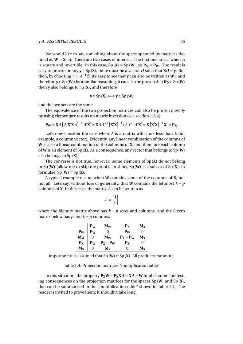
1.A. ASSORTED RESULTS 35
We would like to say something about the space spanned by matrices de-fined as W = X · A. There are two cases of interest. The first one arises when Ais square and invertible: in this case, Sp(X) = Sp(W), so PX = PW. The result iseasy to prove: for any y ∈ Sp(X), there must be a vector β such that Xβ = y. Butthen, by choosing γ = A−1β, it’s easy to see that y can also be written as Wγ andtherefore y ∈ Sp(W); by a similar reasoning, it can also be proven that if y ∈ Sp(W)then y also belongs to Sp(X), and therefore
y ∈ Sp(X) ⇐⇒ y ∈ Sp(W)
and the two sets are the same.The equivalence of the two projection matrices can also be proven directly
by using elementary results on matrix inversion (see section 1.A.4):
PW = XA[
A′X′XA]−1 A′X′ = XA A−1 [
X′X]−1 (A′)−1 A′X′ = X
[X′X
]−1 X′ = PX.
Let’s now consider the case when A is a matrix with rank less than k (forexample, a column vector). Evidently, any linear combination of the columns ofW is also a linear combination of the columns of X, and therefore each columnof W is an element of Sp(X). As a consequence, any vector that belongs to Sp(W)also belongs to Sp(X).
The converse is not true, however: some elements of Sp(X) do not belongto Sp(W) (allow me to skip the proof). In short, Sp(W) is a subset of Sp(X); informulae, Sp(W) ⊂ Sp(X).
A typical example occurs when W contains some of the columns of X, butnot all. Let’s say, without loss of generality, that W contains the leftmost k − pcolumns of X. In this case, the matrix A can be written as
A =[
I0
]where the identity matrix above has k − p rows and columns, and the 0 zeromatrix below has p and k −p columns.
PW MW PX MX
PW PW 0 PW 0MW 0 MW PX −PW MX
PX PW PX −PW PX 0MX 0 MX 0 MX
Important: it is assumed that Sp(W) ⊂ Sp(X). All products commute.
Table 1.4: Projection matrices “multiplication table”
In this situation, the property PXW = PXXA = XA = W implies some interest-ing consequences on the projection matrices for the spaces Sp(W) and Sp(X),that can be summarised in the “multiplication table” shown in Table 1.4. Thereader is invited to prove them; it shouldn’t take long.
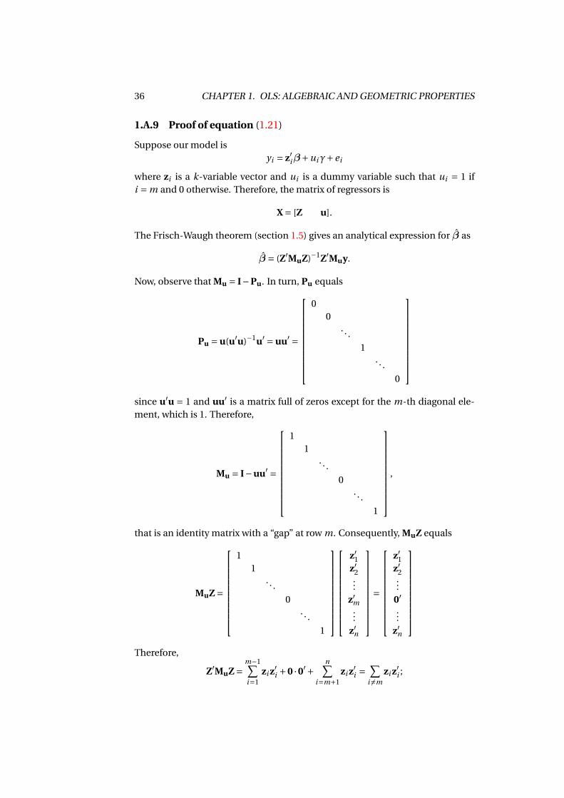
36 CHAPTER 1. OLS: ALGEBRAIC AND GEOMETRIC PROPERTIES
1.A.9 Proof of equation (1.21)
Suppose our model isyi = z′iβ+uiγ+ei
where zi is a k-variable vector and ui is a dummy variable such that ui = 1 ifi = m and 0 otherwise. Therefore, the matrix of regressors is
X = [Z u].
The Frisch-Waugh theorem (section 1.5) gives an analytical expression for β as
β = (Z′MuZ)−1Z′Muy.
Now, observe that Mu = I−Pu. In turn, Pu equals
Pu = u(u′u)−1u′ = uu′ =
00
. . .
1. . .
0
since u′u = 1 and uu′ is a matrix full of zeros except for the m-th diagonal ele-ment, which is 1. Therefore,
Mu = I−uu′ =
11
. . .
0. . .
1
,
that is an identity matrix with a “gap” at row m. Consequently, MuZ equals
MuZ =
11
. . .
0. . .
1
z′1z′2...
z′m...
z′n
=
z′1z′2...
0′...
z′n
Therefore,
Z′MuZ =m−1∑i=1
zi z′i +0 ·0′+n∑
i=m+1zi z′i =
∑i 6=m
zi z′i ;
1.A. ASSORTED RESULTS 37
the expression Z′Muy =∑i 6=m zi yi follows by a totally analogous argument. There-
fore,
β =[ ∑
i 6=mzi zi
]−1 ∑i 6=m
zi yi .
I’ll leave it to the reader, as an exercise, to prove that
γ= em
1−z′m(Z′Z)−1zm,
where em is the m-th element of the vector of residuals that you get from theregression of y on Z on the full sample.

38 CHAPTER 1. OLS: ALGEBRAIC AND GEOMETRIC PROPERTIES
Chapter 2
Some statistical inference
2.1 Why do we need statistical inference?
So far, we have followed a purely descriptive approach, trying to find the smartestpossible method for compressing as much information as we can from the orig-inal data into a small, manageable container.
However, we are often tempted to read the evidence we have in a broadercontext. Strictly speaking, any statistic we compute on a body of data tells ussomething about those data, and nothing else. Thus, the OLS coefficients wecompute are nothing but a clever way to squeeze the relevant information outof our dataset; however, we would often like to interpret the size and the mag-nitudes of the coefficients that we get out of our OLS calculations as somethingthat tells us a more general story. In other words, we would like to perform whatin philosophical language is known as induction.
DAVID HUME
In the 18th century, the Scottish philosopher DavidHume famously argued against induction.
That the sun will not rise tomorrow is no lessintelligible a proposition, and implies no morecontradiction, than the affirmation, that it willrise. We should in vain, therefore, attempt todemonstrate its falsehood. Were it demonstra-tively false, it would imply a contradiction, andcould never be distinctly conceived by the mind.1
Inductive reasoning can be broadly formalised as follows:
1. Event X has always happened in the past.
2. The future will be like the past.
3. Therefore, event X will happen in the future.
1D. Hume, An Enquiry Concerning Human Understanding (1772).
39
40 CHAPTER 2. SOME STATISTICAL INFERENCE
Even if you could establish statement 1 beyond any doubt, statement 2 is ba-sically an act of faith. You may believe in it, but there is no rational argument onecould convincingly use to support it. And yet, we routinely act on the premise ofstatement 2. Hume considered our natural tendency to rely on it as a biologicalfeature of the human mind. And it’s a good thing: if we didn’t have this fun-damental psychological trait, we’d be unable to learn anything at all;2 the onlyproblem is, it’s logically unfounded.
Statistical inference is a way to make an inductive argument more rigorousby replacing statement number 2 with some assumptions that translate into for-mal statements our tendency to generalise, by introducing uncertainty into thepicture. Uncertainty is the concept we use to handle situations in which ourknowledge is partial. So for example we cannot predict which number will showup when we roll a die, although in principle it would be perfectly predictablegiven initial conditions the laws of physics. We simply don’t have the resourcesto perform such a monster computation, so we represent our imperfect knowl-edge through the language of probability, or, more correctly, via a probabilisticmodel; then, we assume that the same model will keep being valid in the future.Therefore, if we rolled a die 10 times and obtained something like
x = [1,5,4,6,3,3,2,6,3,4]
we would act on the assumption that if we keep rolling the same die we willobserve something that, in our eyes, looks “just as random” as x. To put it differ-ently, our aim will not be to predict exactly which side the die will land on, butrather to make statements on how surprising or unsurprising certain outcomeswill be.
Therefore, we use the idea of a Data Generating Process, or DGP. We assumethat the DGP is the mechanism that Nature (or any divinity of your choice) hasused to produce the data we observe, and will continue doing so for the datawe have not observed yet. By describing the DGP via a mathematical structure(usually, but not necessarily, via a probability distribution), we try to come upwith statistics T (x) whose aim is not as much to describe the available data x,but rather to describe the DGP that generated x, and therefore, to provide uswith some insight that goes beyond merely descriptive statistics.
Of course, in order to accomplish such an ambitious task, we need a set oftools to represent imperfect knowledge in a mathematical way. This is why weneed probability theory.
2.2 A crash course in probability
Disclaimer: in this section, I’ll just go quickly though a few concepts that thereader should already be familiar with; as a consequence, it is embarrassingly
2To be fair, this only applies to what Immanuel Kant called “synthetic” propositions. But maybeI’m boring you?

2.2. A CRASH COURSE IN PROBABILITY 41
simplistic and probably quite misleading in many ways. The reader who wantsto go for the real thing might want to read (in increasing order of difficulty): Gal-lant (1997); Bierens (2011); Davidson (1994); Billingsley (1986). Having said this,let’s go ahead.
2.2.1 Probability and random variables
ANDREJ
NIKOLAEVIC
KOLMOGOROV
The concept of probability has been the object of philo-sophical debate for centuries. The meaning of probabilityis still open for discussion,3 but fortunately the syntax ofprobability is clear and undisputed since the great Sovietmathematician Andrej Nikolaevic Kolmogorov made prob-ability a proper branch of measure theory.
The meaning I give to the word probability here islargely operational: probability is a number between 0 and1 that we attach to something called an event. Looselyspeaking, an event is a statement that in our eyes could beconceivably true or false. Formally, an event is defined as asubset of an imaginary set, called the state space, and usu-ally denoted by the letter Ω, whose elements ω are all thestates of the world that our mind can conceive as possible.Probability is a function of subsets ofΩ, which obeys a few properties the readershould already know, such as
P (Ω) = 1, P (;) = 0, P (A∪B) = P (A)+P (B)−P (A∩B)
and so forth. Event A can be defined as the subset of Ω including all the statesω in which a statement A is true, and only those. P (A) is the measure of A,where the technical word “measure” is a generalisation of our intuitive notion of“extension” (length, area, volume).4 The familiar laws of probability are simpleconsequences of the way usual set operations (complement, union, intersec-tion) work; let’s waste no time on those.5
Random variables are a convenient way to map events to segments on thereal line. That is, a random variable X is defined as a measurable function fromΩ to R; or, to put it differently, for any ω inΩ you get a corresponding real num-ber X (ω). The requisite of measurability is necessary to avoid paradoxical cases,and simply amounts to requiring that, if we define A as the the subset ofΩ suchthat
a < X (ω) ≤ b ⇐⇒ω ∈ A,
3The interested reader might want to have a look at Freedman and Stark (2016), section 2. Youcan download it from https://www.stat.berkeley.edu/~stark/Preprints/611.pdf.
4Warning: not all subsets can be associated with a corresponding probability: some are “non-measurable”. Providing a simple example is difficult, this is deep measure theory: google “Vitaliset” if you’re curious.
5In most cases, intuition will suffice. For tricky cases, I should explain what a σ-algebra is, butI don’t think that this is the right place for this, really.
42 CHAPTER 2. SOME STATISTICAL INFERENCE
then A is a proper event. In practice, it must be possible to define P (a < X ≤ b)for any a and b. I will sometimes adopt the convention of using the acronym“rv” for random variables.
There are two objects that a random variable comes equipped with: the firstis its support, which is the subset of R with all the values that X can take; informulae, X : Ω 7→ S ⊆ R, and the set S is sometimes indicated as S(X ). For asix-sided die, S(X ) = 1,2,3,4,5,6; if X is the time before our car breaks down,then S(X ) = [0,∞), and so on.
The other one is its distribution function, or cumulative distribution func-tion (often abbreviated as cdf), defined as
FX (a) = P (X ≤ a),
which of course makes it easy to compute the probability of X being inside aninterval as
P (a < X ≤ b) = FX (b)−FX (a).
By their definition, cdfs enjoy three basic properties:
• lima→−∞ FX (a) = 0;
• lima→∞ FX (a) = 1;
• FX (a) is non-decreasing.
Apart from this, there’s very little that can be said in general. However, in manycases it is assumed that FX (a) has a known functional form, which depends ona vector of parameters θ.
Two special cases are of interest:
1. The cdf is a function that goes up in steps; the support is a countable set,and the corresponding rv is said to be discrete; for every member of thesupport x it is possible to define p(x) = P (X = x) > 0; the function p(x) isthe so-called probability function.
2. The cdf is everywhere differentiable; the support is an interval on R, (pos-sibly, the whole real line), and the corresponding rv is said to be continu-ous; the derivative of Fx (a) is known as the density function of X , or fX (a)and therefore, by definition,
P (a < X ≤ b) =∫ b
afX (z)dz;
in most cases, when the meaning is clear from the context, we just writethe density function for X as f (x).6
6I imagine the reader doesn’t need reminding that the density at x is not the probability thatX = x; for continuous random variables, the probability is only defined for intervals by the for-mula in the text, from which it follows that P (X = x) is 0.
2.2. A CRASH COURSE IN PROBABILITY 43
In the rest of the book, I will mostly use continuous random variables for exam-ples; hopefully, generalisations to discrete rvs should be straightforward.
Of course, you can collect a bunch of random variables into a vector, so youhave a multivariate random variable, or random vector. The multivariate ex-tension of the concepts I sketched above is a little tricky from a technical view-point, but for our present needs intuition will again suffice. I will only mentionthat for a multivariate random variable x with k elements you have that
Fx(a) = P [(x1 ≤ a1)∩ (x2 ≤ a2)∩ . . .∩ (xk ≤ ak )]
If all the k elements of x are continuous random variables, then you can definethe joint density as
fx(z) = ∂k Fx(z)
∂z1∂z2 · · ·∂zk.
The marginal density of the i -th element of x is just the density of xi taken in iso-lation. For example, suppose you have a trivariate random vector w = [X ,Y , Z ]:the marginal density for Y is
fY (a) =∫
S(X )
∫S(Z )
fw(x, a, z)dz dx
2.2.2 Independence and conditioning
If P (A) is the probabilistic evaluation we give of A, we may ask ourselves if wewould change our mind when additional information becomes available. If weare given the news that event B had occurred, then we can safely exclude theevent B from Ω.7 In fact, after receiving the message “B is true”, the state spaceΩ shrinks to B , because states in which B is false are no longer conceivable aspossible.
The consequence for A is that the subset A ∩ B is no longer possible, sowe must update our probability measure so that P (B) becomes 1, and conse-quently8 P (A) must be revised as
P (A|B) ≡ P (A∩B)
P (B)
You read the left-hand side of this definition as “the probability of A given B”,which is of course what we call conditional probability. It should be clear that
P (A) = P (A|B) ⇐⇒ P (A∩B) = P (A) ·P (B)
Which means: “if you don’t need to revise your evaluation of A after havingreceived some message about B , then A and B have nothing to do with each
7When speaking about sets, I use the bar to indicate the complement.8Technically, it’s more complicated that this, because P (B) may be 0, in which case the defini-
tion has to be adapted and becomes more technical. If you’re interested, chapter 10 in Davidson(1994) is absolutely splendid.
44 CHAPTER 2. SOME STATISTICAL INFERENCE
other”; in this situation, A and B are said to be independent, and we write A ⊥⊥ B ,so independence can be thought of as lack of mutual information.
The same concept can be applied to random variables. If
FY (z) = FY (z|a < X ≤ b)
for any a and b, then evidently X carries no information about Y , and we saythat the two random variables are independent: Y ⊥⊥ X .
If this is not the case, it makes sense to consider the conditional distributionof Y on X , which describes our uncertainty about Y once we have informationabout X . So for example, if Y is the yearly expenditure on food by a householdand X is the number of its components, it seems safe to say that F (Y |X > 6)should be different from F (Y |X < 3), because more people eat more food.
The case a = b is important9, because it gives us a tool for evaluating proba-bilities about Y in a situation when X is not uncertain at all, because in fact weobserve its realisation X = x. In this case, we can define the conditional densityas
fY |X=x (z) = fY ,X (z, x)
fX (x)(2.1)
and when what we mean is clear from the context, we simply write f (y |x).Therefore, in many cases we will use the intuitive notion of X , the set of
random variables we are conditioning Y on, as being “the relevant informationabout Y that we have”; in certain contexts, this idea is expressed by the notionof an information set. However, a formalised description of this idea is, again,far beyond the scope of this book and I am contented to leave this to the reader’sintuition.
2.2.3 Expectation
The expectation of a random variable is a tremendously important concept.A rigorous definition, valid in all cases, would require a technical tool calledLebesgue integral, that I’d rather avoid introducing. Luckily, in the two elemen-tary special cases listed in section 2.2.1, its definition is quite simple:
E[X ] =∑
x∈S(X )x ·p(x) for discrete rvs (2.2)
E[X ] =∫
S(X )z · fX (z)dz for continuous rvs. (2.3)
The expectation of a function of X , E[h(X )], is defined simply as
E[h(X )] =∫
S(X )h(z) · fX (z)dz
9Albeit special: a moment’s reflection is enough to convince the reader that if X is continuous,the event X = x has probability 0, and our naïve definition of conditioning breaks down. Butagain, treating the subject rigorously implies using measure theory, σ-algebras and other toolsthat I’m not willing to use in this book.
2.2. A CRASH COURSE IN PROBABILITY 45
for continuous random variables and the parallel definition for the discrete caseis obvious. The extension to multivariate rvs should also be straightforward: theexpectation of a vector is the vector of expectations.
Some care must be taken, since E[X ] may not exist, even in apparently harm-less cases.
Example 2.1If X is a uniform continuous random variable between 0 and 1, its density func-tion is f (x) = 1 for 0 < x ≤ 1. Its expectation is easy to find as
E[X ] =∫ 1
0x ·1dx =
[x2
2
]1
0= 1/2;
however, it’s not difficult to prove that E[1/X ] does not exist (the correspondingintegral diverges):
E[1/X ] =∫ 1
0
1
x·1dx = [
log x]1
0 =∞.
However, it can be proven that if the support of X is finite, then E[X ] is al-ways bounded, and therefore exists. To be more specific: if S(X ) = [a,b], wherea and b are finite, then a < E[X ] < b. The proof is easy and left to the reader asan exercise.
The expectation operator E[·] is linear, and therefore we have the followingsimple rule for affine transforms (A and b must be non-stochastic):
E[Ax+b] = A ·E[x]+b (2.4)
For nonlinear transformation, things are not so easy. As a rule, E[g (X )
] 6= g [E[X ]],and there’s very little you can say in general.10
The expectation of the k-th power of X is called its k-th moment, so the firstmoment is E[X ], the second moment is E
[X 2
]and so on. Of course, E[X n] (with
n ≥ 1) may not exist, but if it does then E[
X n−1]
is guaranteed to exist too.The most egregious example of usefulness of moments is the definition of
variance:11 V[X ] = E[
X 2]−E[X ]2. The variance is always non-negative, and is
the most widely used indicator of dispersion. Of course, in order to exist, the sec-ond moment of X must exist. Its multivariate generalisation is the covariancematrix, defined as
Cov[x] = E[xx′
]−E[x]E[x]′ ; (2.5)
10In fact, there is something more general we can say, when the transformation g (X ) is concaveon the whole support of X : it’s called Jensen’s lemma. We will not use this result in this book, butthe result is widely used in economics and econometrics; if you’re interested, the idea is brieflyexplained in section 2.A.1.
11An alternative equivalent definition, perhaps more common, is V[X ] = E[(X −E[X ])2]
.
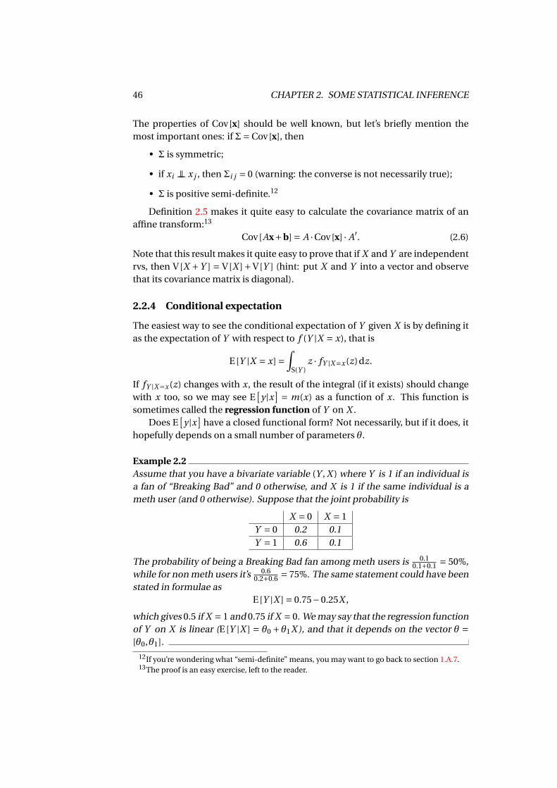
46 CHAPTER 2. SOME STATISTICAL INFERENCE
The properties of Cov[x] should be well known, but let’s briefly mention themost important ones: if Σ= Cov[x], then
• Σ is symmetric;
• if xi ⊥⊥ x j , then Σi j = 0 (warning: the converse is not necessarily true);
• Σ is positive semi-definite.12
Definition 2.5 makes it quite easy to calculate the covariance matrix of anaffine transform:13
Cov[Ax+b] = A ·Cov[x] · A′. (2.6)
Note that this result makes it quite easy to prove that if X and Y are independentrvs, then V[X +Y ] = V[X ]+V[Y ] (hint: put X and Y into a vector and observethat its covariance matrix is diagonal).
2.2.4 Conditional expectation
The easiest way to see the conditional expectation of Y given X is by defining itas the expectation of Y with respect to f (Y |X = x), that is
E[Y |X = x] =∫
S(Y )z · fY |X=x (z)dz.
If fY |X=x (z) changes with x, the result of the integral (if it exists) should changewith x too, so we may see E
[y |x] = m(x) as a function of x. This function is
sometimes called the regression function of Y on X .Does E
[y |x]
have a closed functional form? Not necessarily, but if it does, ithopefully depends on a small number of parameters θ.
Example 2.2Assume that you have a bivariate variable (Y , X ) where Y is 1 if an individual isa fan of “Breaking Bad” and 0 otherwise, and X is 1 if the same individual is ameth user (and 0 otherwise). Suppose that the joint probability is
X = 0 X = 1Y = 0 0.2 0.1Y = 1 0.6 0.1
The probability of being a Breaking Bad fan among meth users is 0.10.1+0.1 = 50%,
while for non meth users it’s 0.60.2+0.6 = 75%. The same statement could have been
stated in formulae asE[Y |X ] = 0.75−0.25X ,
which gives 0.5 if X = 1 and 0.75 if X = 0. We may say that the regression functionof Y on X is linear (E[Y |X ] = θ0 +θ1X ), and that it depends on the vector θ =[θ0,θ1].
12If you’re wondering what “semi-definite” means, you may want to go back to section 1.A.7.13The proof is an easy exercise, left to the reader.
2.3. ESTIMATION 47
Of course, if x is a random variable, m(x) is too. Does it have an expectation?If so,
E[E
[y |x]]= E
[y]
. (2.7)
This is called law of iterated expectations, and is in fact more general thanit appears at first sight. For example, it applies to density functions too:
f (y) = E[
f (y |x)]
To continue with example 2.2, note that E[Y ] = E[0.75−0.25 ·X ] = 0.75−0.25 ·E[X ] = 0.7.
It must be stressed that expressing the relationship between two randomvariables by means of the conditional expectation has no meaning on causalrelationship. Example 2.2 above should not be taken to imply that if you startdoing meth you grow a dislike for that certain TV series. However, this does notmean that it’s not worth examining. More on this in Section 3.1.
2.3 Estimation
The best way to define the concept of an estimator is to assume that we observesome data x, and that the DGP which generated x can be described by meansof a vector of parameters θ. An estimator is a statistic θ = T (x) that should be“likely” to yield a value “close to” the parameters of interest θ.
To state the same idea more formally: θ is a function of x, so it is a randomvariable too, and therefore has a support and a distribution function. Clearly,both will depend on those of x, but ideally, we’d like to choose the function T (·)so that the support S(θ) contains at least a neighbourhood of θ, and we’d likeP (θ−ε< θ < θ+ε) = P (|θ−θ| < ε) to be as close to 1 as possible.
In very simple cases,14 we may be able to compute E[θ]
and perhaps evenV
[θ], which leads us to the well known concepts of unbiasedness and efficiency:
• the bias of θ is the difference E[θ]−θ; therefore θ is said to be unbiased if
E[θ]= θ;
• θ is more efficient than θ if V[θ]−V
[θ]> 0 (if both are unbiased).
The problem that makes these concepts not very useful is that, in many cases ofinterest, it’s very hard, if not impossible, to compute the moments of θ (in somecases, θ may even possess no moments at all). So we need to use something else.Fortunately, asymptotic theory comes to the rescue.
14Notably, when θ is an affine function of x.
48 CHAPTER 2. SOME STATISTICAL INFERENCE
2.3.1 Consistency
The estimator θ is consistent if its probability limit is the parameter we want toestimate. To explain what this means, let us first define convergence in proba-bility:
Xnp−→ X ⇐⇒ lim
n→∞P [|Xn −X | < ε] = 1 (2.8)
Also notated as plim(Xn) = X .A description in words of the definition above is: given a sequence of random
variables X1, X2, . . . , Xn , we define a parallel sequence of events of the kind
|X1 −X | < ε, |X2 −X | < ε, . . . , |Xn −X | < ε;
the sequence above can be read as a sequence of events, where |Xi − X | < ε
means “Xi is more or less X ”.15 Convergence in probability means that the se-quence of probabilities for those events tends to 1; that is, the probability of Xn
and X being “substantially different” becomes negligible if n is large.16
In general, the limit X could be a random variable, but we’ll be mostly in-
terested in the case when the limit is a constant: if Xnp−→ a, the chances of
Xn being far from a become zero, and therefore the cdf of Xn tends to a stepfunction which is 0 before a and 1 after it. Or, if Xn is continuous, the densityfunction f (Xn) collapses to a point.
This is exactly what happens, in many circumstances, when we compute thesample average in a data set. Imagine you have n observations: you can com-pute the average of the observations you have as they become available; thatis,
X1 = X1, X2 = X1 +X2
2, X3 = X1 +X2 +X3
3, · · · ;
does the sequence Xn have a limit in probability? The conditions for this arestudied by the so-called Laws of Large Numbers, or LLNs for short.17
There are many LLNs, and they cover different cases. Basically, there arethree dimensions to the problem that must be considered:
1. How heterogeneous are the Xi variables?
2. Are the Xi variables independent?
3. Can we assume the existence of at least some of the moments?
The simplest version of the LLN is Khinchin’s, which sets very strong boundson the first two conditions and relaxes the third one as much as possible: ifx1, x2, . . . , xn are independent and identically distributed (iid for short) and E[xi ] =
15Where ε> 0 is the mathematically respectable way of saying “more or less”.16The curious reader might be interested in knowing that there are several other ways to define
a similar concept. A particularly intriguing one is the so-called “almost sure” convergence.17Technically, these are the weak LLNs. The strong version uses a different concept of limit.
2.3. ESTIMATION 49
m, then Xp−→ m. Other versions exist: for example, a different version of the
LLN can be used if observations are not independent, but in that case morestringent assumptions are needed; allow me to skip these complications.
Example 2.3Let’s toss a coin n times. The random variable representing the i -th toss is xi ,which is assumed to obey the following probability distribution:
xi =
1 with probability π0 with probability 1−π
Not that the probabilityπ is assumed to be the same for all xi ; that is, the coin wetoss does not change its physical properties during the experiment. Moreover, itis safe to assume that what happens at the i -th toss has no consequences on allthe other ones. In short, the xi random variables are iid.
Does xi have a mean? Yes: E[xi ] = 1 ·π+0 · (1−π) = π. Together with the iid
property, this is enough for invoking the LLN and establishing that X = pp−→ π.
Therefore, we can take the empirical frequency p as a consistent estimator ofthe true probability π.
Another common case when it’s easy to prove convergence in probabilityoccurs when each member of the sequence xi possesses finite second momentsand
limn→∞E[xi ] = m
limn→∞V[xn] = 0;
if m is finite, there is a result called Chebyshev’s inequality, using which you
can easily prove that Xp−→ m. This case is nearly useless in practice because
being able to compute the moments of our quantities of interest is extremelyrare, but still gives you a nice idea of the kind of conditions you can use to proveconsistency.
The LLN becomes enormously powerful when coupled with another won-
derful result, known as the Slutsky’s Theorem: if Xnp−→ a and g (·) is continuous
at a, then g (Xn)p−→ g (a) (note how much easier this property makes it to work
with probability limits rather than expectations).We will want our estimators to be consistent:
θp−→ θ⇐⇒ lim
n→∞P[|θ−θ| < ε]= 1; (2.9)
that is, we will want to use as estimators statistics that become increasingly un-likely to be grossly wrong.
Fortunately, the combination of the LLN and Slutsky’s Theorem provides avery nice way to construct estimators that are consistent by construction. If the
50 CHAPTER 2. SOME STATISTICAL INFERENCE
average has a probability limit that is a continuous, invertible function of theparameter we want, we just apply a suitable transformation the the average andwe’re done: so for example if E[xi ] = 1/θ, then θ = 1/X ; if E[xi ] = eθ, then θ =log(X ); if E[xi ] = θ2, then θ =
√X ; and so on. The extension to the case when θ
is a vector is technically messier, but conceptually identical.
Example 2.4Suppose you have a sample of iid random variables for which you know that
E[X ] = p
α
E[
X 2] = p(p +1)
α2 ;
and define the two statistics m1 = X = n−1 ∑i xi and m2 = n−1 ∑
i x2i . Clearly
m1p−→ p
α
m2p−→ p(p +1)
α2 .
Now consider the statistic p = m21
m2−m21
. Clearly p is a continuous function of
both m1 and m2; therefore,
p = m21
m2 −m21
p−→ p2/α2
p(p +1)/α2 −p2/α2 = p2
p2 +p −p2 = p,
So p is a consistent estimator of p.But then, by the same token, by dividing p by m1 you get that
p
m1= m1
m2 −m21
p−→ p
p/α=α,
so you get a second statistic, α= m1
m2−m21
which estimates α consistently.
2.3.2 Asymptotic normality
Consistency is important because we want our estimators to be reasonably pre-cise for large samples, but this is almost never enough, as we may need to makemore precise statements on the distribution of our estimators. For example:imagine that we have 2 consistent estimators from the same quantity: that is,two different statistics θ and θ that have the same probability limit θ.
How do we choose which one to use? Consistency can’t be a criterion, sincethey both are: if we define
Pn = P[|θ−θ| < ε]
Pn = P[|θ−θ| < ε]
2.3. ESTIMATION 51
clearly limn→∞ Pn = limn→∞ Pn = 1, so a decision can’t be made on these grounds.Nevertheless, if we could establish that, for n large enough, Pn > Pn , so that ourprobability of being grossly wrong is lower if we use θ instead of θ, our preferredcourse of action would be obvious. Unfortunately, this is not an easy check: Pn
is defined as
Pn =∫ θ+ε
θ−εf (x)dx,
where f (x) is the density function for θ (clearly, a parallel definition holds forPn). In most cases, the analytical form of f (x) is very hard to establish, if not atall impossible. However, it may be possible to find approximations to the actualdensities that are good enough to perform the required check. This is almostinvariably achieved by resorting to a property called asymptotic normality, bywhich the unknown density f (x) can be approximated via a suitably chosenGaussian density.18
At first sight, this sounds like a very ambitious task: how can we hope tomake general statements on the distribution of an arbitrary function of arbi-trarily distributed random variables? And yet, there is a result that applies in asurprisingly large number of cases, and goes under the name of Central LimitTheorem, or CLT for short.
Basically, the CLT says that, under appropriate conditions, when you observea random variable X that can be conceivably thought of as the accumulation ofa large number of random causes that are reasonably independent of each otherand with none of them dominating the others in magnitude, there are very goodchances that the distribution of X should be approximately normal.
HENRI POINCARÉ
The practical effect of this theorem is ubiquitous innature; most natural phenomena follow (at least approx-imately) a Gaussian distribution; the width of leaves, thelength of fish, the height of humans. The French mathe-matician Henri Poincaré is credited with the following re-mark:
Everyone is sure of this, Mr. Lippman toldme one day, since the experimentalists be-lieve that it is a mathematical theorem, andthe mathematicians that it is an experimen-tally determined fact.19
In order to illustrate the concept, we have to begin by defining convergencein distribution:
Xnd−→ X ⇐⇒ FXn (z) → FX (z) (2.10)
18I assume that the reader is reasonably comfortable with the Gaussian distribution, but section2.A.2 is there, just in case.
19French original: Tout le monde y croit cependant, me disait un jour M. Lippmann, car les ex-périmentateurs s’imaginent que c’est un théorème de mathématiques, et les mathématiciens quec’est un fait expérimental.
52 CHAPTER 2. SOME STATISTICAL INFERENCE
When Xn converges in distribution to X , the difference between P (a < Xn ≤b) and P (a < X ≤ b) becomes negligible for large n. So, for large n, we can ap-proximate quite accurately the probability of events defined for Xn via the corre-
sponding event defined for X . It can be proven that Xnp−→ X implies Xn
d−→ X ,but not vice versa.
Note the fundamental difference between convergence in probability and in
distribution: if Xnp−→ X , then for large n each time we observe a realisation of
Xn and X we can be fairly confident that the two numbers will be very close.
If Xnd−→ X instead, there is no guarantee that the two numbers will be close:
the only thing we know is that they come from (nearly) the same probabilitydistribution.
Now imagine that the LLN holds and Xp−→ m. Clearly, X −m
p−→ 0. In manycases, it can be proven that multiplying that quantity by
pn gives you something
that doesn’t collapse to 0 but does not diverge to infinity either. The CentralLimit Theorems analyses the conditions under which
pn(X −m)
d−→ N (0, v), (2.11)
where N (0, v) is a Gaussian random variable. A multivariate version also exists,which is slightly more intricate from a technical point of view, but the intuitioncarries over straightforwardly.
The approximation provided by the CLT can also be stated by using the sym-bol a∼ , which means “approximately distributed as” (where the approximationgets better and better as n grows):
pn (x−m)
d−→ N (0,Σ) =⇒ x a∼ N
(m,
1
nΣ
)In the same way as the LLN, there are many versions of the CLT, designed
to cover different cases. A simple version, close in spirit to Khinchin’s LLN,was provided by Lindeberg and Lévy: if x1, x2, . . . , xn are iid, E[xi ] = m, andV[xi ] = v , then equation (2.11) holds. In practice, the conditions are the same asin Khinchin’s LLN, with the additional requirement that the variance of xi mustexist.
Example 2.5Let’s go back to example 2.3 (the coin-tossing experiment). Here not only themean exists, but also the variance:
V[xi ] = E[x2
i
]−E[xi ]2 =π−π2 =π(1−π)
Therefore, the Lindeberg-Lévy version of the CLT is readily applicable, and wehave p
n(p −π)d−→ N (0,π(1−π)),
2.3. ESTIMATION 53
so the corresponding asymptotic approximation is
p a∼ N
(π,π(1−π)
n
).
In practice, if you toss a fair coin (π = 0.5) n = 100 times, the distributionof the relative frequency you get is very well approximated by a Gaussian ran-dom variable with mean 0.5 and variance 0.0025. Just so you appreciate howwell the approximation works, consider that the event 0.35 < p ≤ 0.45 has a trueprobability of 18.234%, while the approximation the CLT gives you is 18.219%. Ifyou’re interested in reproducing these numbers, Section 2.A.3 contains a smallgretl script with all the necessary steps. Of course, you’re strongly encouraged totranslate it to any other software you like better.
The CLT, by itself, describes the convergence in distribution of averages. How-ever, we need to see what happens to our estimators, that are usually functionsof those averages. There are two tools that come in especially handy. The first
one is sometimes called Cramér’s theorem: if Xnp−→ a and Yn
d−→ Y , then
Xn ·Ynd−→ a ·Y . (2.12)
The second result we will often use is the delta method: if your estimator θ isdefined as a differentiable transformation of a quantity which obeys a LLN anda CLT, there is a relatively simple rule to obtain the limit in distribution of θ;
Xp−→ m
pn
(X −m
) d−→ N (0,Σ)
=⇒
θ = g (X )
p−→ θ = g (m)p
n(θ−θ) d−→ N (0, JΣJ ′)
(2.13)
where n is the sample size and J is the Jacobian ∂g (x)∂x
∣∣∣x=m
.
Example 2.6Given a sample of iid random variables xi for which E[xi ] = 1/a and V[xi ] =1/a2, it is straightforward to construct a consistent estimator of the parameter aas
a = 1
X
p−→ 1
1/a= a.
Its asymptotic distribution is easy to find: start from the CLT:
pn
(X −1/a
) d−→ N (0,1/a2).
All we need is the Jacobian term, which is
J = plimda
dX=−plim
1
X 2=− 1
1/a2 =−a2;
54 CHAPTER 2. SOME STATISTICAL INFERENCE
therefore, the variance of the asymptotic distribution of a is given by20
AV[a] = (−a2)1
a2 (−a2) = a2,
and therefore pn (a −a)
d−→ N (0, a2)
so we can use the approximation a a∼ N(a, a2
n
).
By using these tools, we construct estimators satisfying not only the consis-tency property, but also asymptotic normality. These estimators are sometimestermed CAN estimators (Consistent and Asymptotically Normal). Asymptoticnormality is important for two reasons:
1. it can be used to compare two consistent estimators in terms of their rel-ative asymptotic efficiency. Given two consistent estimators a and b forthe same parameter m, we’ll say that a is asymptotically more efficientthan b if AV[b]−AV[a] is positive semi-definite (see page 34). This cri-terion is easy to understand when a and b are scalars: AV[b] ≥ AV[a].The vector case is more subtle: if our object of interest is estimating somescalar function of m (say, g (m)), then the two natural competing estima-tors would be g (a) and g (b), respectively, that are both consistent by Slut-sky’s theorem. However, by applying the delta method, it can be proventhat AV
[g (b)
]≥ AV[g (a)
]in all cases.
2. It provides a fairly general way to construct statistics for testing hypothe-ses, which is probably the most useful thing an applied scientist mightwant to do with data. The next section is just about this.
In addition, asymptotic normality makes it quite easy to construct confi-dence intervals: in order to illustrate the concept, suppose we have a scalar es-timator θ, whose asymptotic distribution is
pn
(θ−θ) d−→ N (0,ω);
this means that, for a decently large value of n, we can approximate the distri-bution of θ as θ a∼ N
(θ, ωn
). This, in turn, implies that
P
[|θ−θ|pω/n
> 1.96
]' 5%;
therefore, the chances that the interval
θ±1.96×pω/n
20It is common to call AV[θ]
the “asymptotic variance” of θ; this is technically incorrect, since θmay not have a variance for any n, although its limit distribution does. But let’s not be pedantic.

2.4. HYPOTHESIS TESTING 55
contains the true value of θ are roughly 95%. This is what is called a 95% confi-dence interval. Of course, a 99% confidence interval would be somewhat larger.Generalising this to a vector of parameters would lead us to speaking of con-fidence sets; for example, when θ is a 2-parameter vector, the confidence setwould be an ellipse.
2.4 Hypothesis Testing
The starting point is a tentative conjecture (called the null hypothesis, or H0)that we make about the parameters of a DGP;21 we would like to check whetherour belief is consistent with the observed data. If what we see is at odds with ourhypothesis, then reason dictates we should drop it in favour of something else.
The coin toss is a classic example. We presume that the coin is fair, but it’dbe nice if we could check. What we can do is flip it a number of times, andthen decide, on the basis of the results, if our original conjecture is still tenable.The probability of the coin showing the “heads” side when we flip it (say, π) is anumber between 0 and 1. Our conjecture is H0 : π = 0.5. After flipping the coinn times, we obtain a vector x of zeros and ones. What we want is a function T (x)(called a test statistic) such that we can decide whether to reject H0 or not.
Figure 2.1: Types of Error
Note: in this case, H0 is that the person is not pregnant.
21Disclaimer: this section is horribly simplistic. Any decent statistics textbook is far better thanthis. My aim here is just to lay down a few concepts that I will use in subsequent chapters, with noclaim to rigour or completeness. My advice to the interested reader is to get hold of Casella andBerger (2002) or Gourieroux and Monfort (1995, volume 2). Personally, I adore Spanos’ historicalapproach to the matter.
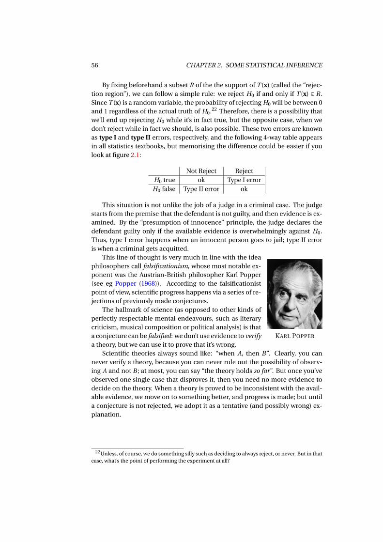
56 CHAPTER 2. SOME STATISTICAL INFERENCE
By fixing beforehand a subset R of the the support of T (x) (called the “rejec-tion region”), we can follow a simple rule: we reject H0 if and only if T (x) ∈ R.Since T (x) is a random variable, the probability of rejecting H0 will be between 0and 1 regardless of the actual truth of H0.22 Therefore, there is a possibility thatwe’ll end up rejecting H0 while it’s in fact true, but the opposite case, when wedon’t reject while in fact we should, is also possible. These two errors are knownas type I and type II errors, respectively, and the following 4-way table appearsin all statistics textbooks, but memorising the difference could be easier if youlook at figure 2.1:
Not Reject RejectH0 true ok Type I errorH0 false Type II error ok
This situation is not unlike the job of a judge in a criminal case. The judgestarts from the premise that the defendant is not guilty, and then evidence is ex-amined. By the “presumption of innocence” principle, the judge declares thedefendant guilty only if the available evidence is overwhelmingly against H0.Thus, type I error happens when an innocent person goes to jail; type II erroris when a criminal gets acquitted.
KARL POPPER
This line of thought is very much in line with the ideaphilosophers call falsificationism, whose most notable ex-ponent was the Austrian-British philosopher Karl Popper(see eg Popper (1968)). According to the falsificationistpoint of view, scientific progress happens via a series of re-jections of previously made conjectures.
The hallmark of science (as opposed to other kinds ofperfectly respectable mental endeavours, such as literarycriticism, musical composition or political analysis) is thata conjecture can be falsified: we don’t use evidence to verifya theory, but we can use it to prove that it’s wrong.
Scientific theories always sound like: “when A, then B”. Clearly, you cannever verify a theory, because you can never rule out the possibility of observ-ing A and not B ; at most, you can say “the theory holds so far”. But once you’veobserved one single case that disproves it, then you need no more evidence todecide on the theory. When a theory is proved to be inconsistent with the avail-able evidence, we move on to something better, and progress is made; but untila conjecture is not rejected, we adopt it as a tentative (and possibly wrong) ex-planation.
22Unless, of course, we do something silly such as deciding to always reject, or never. But in thatcase, what’s the point of performing the experiment at all?
2.4. HYPOTHESIS TESTING 57
I am fully aware that the debate on philoso-phy of science has long established that fal-sificationism is untenable, as a description ofscientific progress, on several accounts. WhatI’m saying is just that the statistical thoery of
hypothesis testing borrows quite a few ideasfrom the falsificationist approach. For a fulleraccount, check out Andersen and Hepburn(2016).
Therefore, strictly speaking, “not rejecting” doesn’t mean “accepting”. Rejec-tion is always final; failure to reject is always provisional. That said, it is quitecommon (although incorrect) to use the word “accept” instead of “not reject”,and I will do the same here. However, the reader should bear in mind is that“accepting” really means “accepting for now”.23
The recipe we are going to use for constructing test statistics is simple: first,we will formulate our hypothesis of interest as H0 : g (θ) = 0, where θ are the DGPparameters and g (·) is a differentiable function. Then, given a CAN estimator θ,we evaluate the function at that point. Given consistency, we would expect g (θ)
to be “small” if H0 is true, since under H0, g (θ)p−→ 0.
In order to build a rejection region, we need some criterion for decidingwhen g (θ) is large enough to force us to abandon H0; we do so by exploitingasymptotic normality. By using the delta method, we can find an asymptoticapproximation to the distribution of g (θ) as
g (θ) a∼ N (g (θ),Σ);
under consistency, Σ should tend to a zero matrix; as for g (θ), that should be0 if and only if H0 is true. These two statement imply that the quadratic formg (θ)′Σ−1g (θ) should behave very differently in the two cases: if H0 is false, itshould diverge to infinity, since plim
[g (θ)
] 6= 0; if H0 is true, instead, approxi-mate normality implies that24.
W = g (θ)′Σ−1g (θ) a∼ χ2p
where p = rk(Σ). Hence, under H0, the W statistic should take values typicalof a χ2 random variable.25 Therefore, we should expect to see “small” valuesof W when H0 is true and large values when it’s false. The natural course ofaction is, therefore, to set the rejection region as R = (c,∞), where c, the criticalvalue, is some number to be determined. Granted, there is always the possibilitythat W > c even if H0 is true. In that case, we would be committing a type Ierror. But since we can calculate the distribution function for W , we can set cto a prudentially large value. What is normally done is to set c such that the
23Some people use the word “retain” instead of “accept”, which is certainly more correct, butunfortunately not very common.
24To see why, see section 2.A.225The reason why I’m using the letter W to indicate the test is that, in a less cursory treatment
of the matter, the test statistic constructed in this way could be classified as a “Wald-type” test.
58 CHAPTER 2. SOME STATISTICAL INFERENCE
probability of a type I error (called the size of the test, and usually denoted bythe Greek letter α) is a small number, typically 5%.
What people do in most cases is deciding whichα they want to use and thenset c accordingly, so that in many cases you see c expressed as a function if α(and written cα), rather than the other way around.
But, I hear you say, what about type II error? Well, if W in fact diverges whenH0 is false, the the probability of rejection (also known as the power of the test)should approach 1, and we should be OK, at least when our dataset is reasonablylarge.26 There are many interesting things that could and should be said aboutthe power of tests, especially a truly marvelous result known as the Neyman-Pearson lemma, but I’m afraid this is not the place for this. See the literaturecited at footnote 21.
Example 2.7Let’s continue example 2.5 here. So we have that the relative frequency is a CANestimator for the probability of a coin showing “heads”.
pn(p −π)
d−→ N (0,π(1−π)).
Let’s use this result for building a test for the “fair coin” hypothesis, H0 : π= 0.5.We need a differentiable function g (x) such that g (x) = 0 if and only if x = 0.5.One possible choice is
g (π) = 2π−1
What we have to find is the asymptotic variance of g (p), which is AV[g (p)
]=J ·π(1−π) · J ′ =ω, where J = plim
(∂g (x)∂x
)= 2, so
pn(g (p)− g (π))
d−→ N (0,ω).
Under the null, g (π) = 0 and ω = 1; therefore, the approximate distribution forg (p) is
g (p) a∼ N (0,n−1)
and our test statistic is easy to build as
W = g (p)
[1
n
]−1
g (p) = n · (2p −1)2
A simple numerical example: suppose n = 100 and p = 46%. The value ofW equals W = 100 ·0.082 = 0.64. Is the number 0.64 incompatible with the pre-sumption that the coin is fair? Not at all: if the coin is in fact fair W should comefrom a random variable that in 95% of the cases takes values below 3.84. There-fore, there is no reason to change our mind about H0. The reader may want tocheck what happens if the sample size of our experiment is set to n = 1000.
26When the power of a test goes to 1 asymptotically, the test is said to be consistent. I know, it’sconfusing.
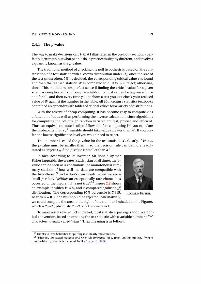
2.4. HYPOTHESIS TESTING 59
2.4.1 The p-value
The way to make decisions on H0 that I illustrated in the previous section is per-fectly legitimate, but what people do in practice is slightly different, and involvesa quantity known as the p-value.
The traditional method of checking the null hypothesis is based on the con-struction of a test statistic with a known distribution under H0; once the size ofthe test (most often, 5%) is decided, the corresponding critical value c is foundand then the realised statistic W is compared to c. If W > c, reject; otherwise,don’t. This method makes perfect sense if finding the critical value for a givensize α is complicated: you compile a table of critical values for a given α onceand for all, and then every time you perform a test you just check your realisedvalue of W against the number in the table. All 20th century statistics textbookscontained an appendix with tables of critical values for a variety of distributions.
With the advent of cheap computing, it has become easy to compute c asa function of α, as well as performing the inverse calculation, since algorithmsfor computing the cdf of a χ2 random variable are fast, precise and efficient.Thus, an equivalent route is often followed: after computing W , you calculatethe probability that a χ2 variable should take values greater than W . If you pre-fer, the lowest significance level you would need to reject.
That number is called the p-value for the test statistic W . Clearly, if W > c,the p-value must be smaller than α, so the decision rule can be more readilystated as “reject H0 if the p-value is smaller than α”.
RONALD FISHER
In fact, according to its inventor, Sir Ronald AylmerFisher (arguably, the greatest statistician of all time), the p-value can be seen as a continuous (or monotonous) sum-mary statistic of how well the data are compatible withthe hypothesis;27 in Fischer’s own words, when we see asmall p-value, “[e]ither an exceptionally rare chance hasoccurred or the theory [...] is not true”.28 Figure 2.2 showsan example in which W = 9, and is compared against a χ2
3distribution. The corresponding 95% percentile is 7.815,so with α = 0.05 the null should be rejected. Alternatively,we could compute the area to the right of the number 9 (shaded in the Figure),which is 2.92%; obviously, 2.92% < 5%, so we reject.
To make results even quicker to read, most statistical packages adopt a graph-ical convention, based on ornating the test statistic with a variable number of ’*’characters, usually called “stars”. Their meaning is as follows:
27Thanks to Sven Schreiber for putting it so clearly and concisely.28Fisher RA. Statistical Methods and Scientific Inference. Ed 2, 1959. On this subject, if you’re
into the history of statistics, you might like Biau et al. (2009).
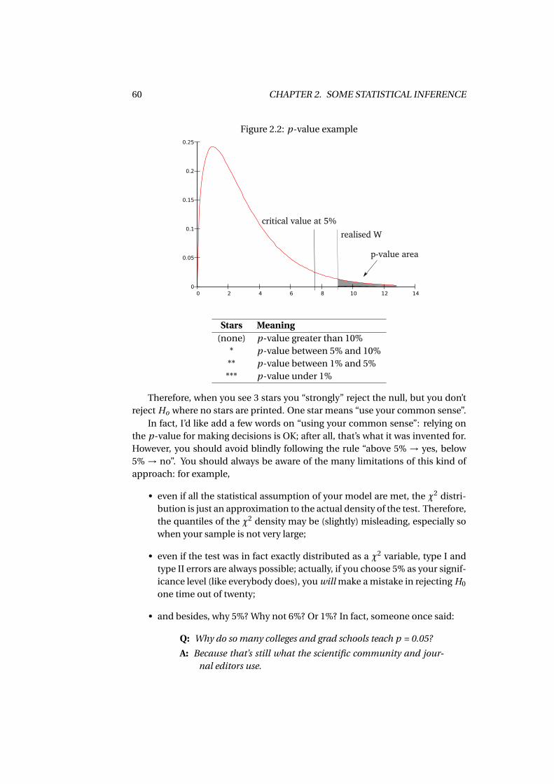
60 CHAPTER 2. SOME STATISTICAL INFERENCE
Figure 2.2: p-value example
critical value at 5%
realised W
p-value area
Stars Meaning(none) p-value greater than 10%
* p-value between 5% and 10%** p-value between 1% and 5%*** p-value under 1%
Therefore, when you see 3 stars you “strongly” reject the null, but you don’treject Ho where no stars are printed. One star means “use your common sense”.
In fact, I’d like add a few words on “using your common sense”: relying onthe p-value for making decisions is OK; after all, that’s what it was invented for.However, you should avoid blindly following the rule “above 5% → yes, below5% → no”. You should always be aware of the many limitations of this kind ofapproach: for example,
• even if all the statistical assumption of your model are met, the χ2 distri-bution is just an approximation to the actual density of the test. Therefore,the quantiles of the χ2 density may be (slightly) misleading, especially sowhen your sample is not very large;
• even if the test was in fact exactly distributed as a χ2 variable, type I andtype II errors are always possible; actually, if you choose 5% as your signif-icance level (like everybody does), you will make a mistake in rejecting H0
one time out of twenty;
• and besides, why 5%? Why not 6%? Or 1%? In fact, someone once said:
Q: Why do so many colleges and grad schools teach p = 0.05?
A: Because that’s still what the scientific community and jour-nal editors use.
2.5. IDENTIFICATION 61
Q: Why do so many people still use p = 0.05?
A: Because that’s what they were taught in college or grad school.
(for more details, see Wasserstein and Lazar (2016)).
That said, I don’t want you to think “ok, the p-value is rubbish”: it isn’t. Ac-tually, it’s the best tool we have for the purpose. But like any other tool (be it ascrewdriver, a microwave oven or a nuclear reactor), in order to use it effectively,you must be aware of its shortcomings.
2.5 Identification
A common problem in econometrics is identification of a model. The issue isquite complex, and I cannot do justice to it in an introductory book such as this,so I’ll just sketch the main ideas with no pretence to rigour or completeness.Basically, a model is said to be identified with reference to a question of interestif the model’s probabilistic structure is informative on that question.
A statistical model is, essentially, a probabilistic description of the data thatwe observe. When we perform inference on a dataset we assume that
• our available dataset is a realisation of some probabilistic mechanism (theDGP — see section 2.1);
• the salient features of the DGP can be described by a parameter vector θ;
• the data we observe are such that asymptotic theory is applicable (for ex-ample, n is large and the data are iid) and we can define statistics that wecan use as estimators or tests;
• our question of interest can be phrased as a statement on the vector θ.
The importance of the first three items in the list should be clear to the readerfrom the past sections of this chapter. In this section, we will discuss the fourthone.
The vector θ contains parameters that describe the probability distributionof our data, but in principle the empirical problem we are ultimately interestedin is expressed as a vector of parameters of interestψ. That is, the parameters θcharacterise the DGP, while ψ is a formalised description of the aspect of realitywe are trying to analyse. For example, in a typical econometric model, ψ maycontain quantities such as the elasticity of demand for a certain good to its ownprice, or to the price of a substitute good, and so on.
What is the relationship between ψ and θ? If we take ψ as being a styliseddescription of reality, and θ as a stylised description of what we observe, then θ
should be a known function of ψ, that we assume known:
θ = M(ψ).
62 CHAPTER 2. SOME STATISTICAL INFERENCE
In some cases, the relationship is trivial; often, M(·) is just the identity function,θ =ψ, but sometimes this is not the case.
Statistics gives us the tools to estimate θ; is this enough to estimate ψ? Itdepends on the function M(·); if the function is invertible, and we have a CANestimator θ, a possible estimator for ψ is
ψ= M−1(θ).
If M(·) is continuous and differentiable, then its inverse will share these prop-erties, so we can use Slutsky’s theorem and the delta method and ψ is a CANestimator too. In this case, we say that the model is identified.
In some cases, however, the function M(·) is not invertible, typically whendifferent values of ψ give rise to the same θ.29. In other terms, two alternativedescriptions of the world give rise to the same observable consequences: if
M(ψ1) = M(ψ2)
forψ1 6=ψ2, we would observe data from the same DGP (described by θ) in bothcases; this situation is known as observational equivalence, and ψ1 and ψ2 aresaid to be observationally equivalent. In these case, being able to estimate θ,even in an arbitrarily precise way, doesn’t tell us if the “true” description of theworld is ψ1 or ψ2. This unfortunate case is known in econometrics as under-identification.
Example 2.8Suppose you have an urn full of balls, some white and some red. Call w thenumber of white balls and r the number of red balls. We want to estimate bothw and r .
The only experiment we can perform works as follows: we can extract oneball from the urn as many times as we want, but we must put it back after ex-traction (statisticians call this “sampling with replacement”). Define the randomvariable xi as 1 if the ball is red. Clearly
xi =
1 with probability π= rw+r
0 with probability (1−πi ) = ww+r
In this case, the probability distribution of our data is completely characterisedby the parameter π; as we know, we have a perfectly good way to estimate π,since X is a consistent estimator and testing hypotheses on π is easy.
If, however, the parameters of interest are ψ = [r, w], there is no way to es-timate them separately, because the function θ = M(ψ) is not invertible, for thevery simple reason that
π= r
w + r
29The technical way to say this would be “the M(·) function is not injective”.
2.A. ASSORTED RESULTS 63
is one equation in two unknowns. Therefore, in the absence of extra informationwe are able to estimateπ (the proportion of red balls) as precisely as wanted, butthere is no way to estimate r (the number of red balls).
Even if we knew the true value ofπ, there sould still be an infinite array of ob-servationally equivalent descriptions of the urn. If, say, π = 0.3 the alternativesψ1 = [3,10], ψ2 = [15,50], ψ3 = [3000,10000], etc would all be observationallyequivalent.
Identification of a model can be a very serious concern in some settings:if a model is under-identified, we may be able to estimate consistently the pa-rameters that describe the data, but this wouldn’t be helpful for the economicquestion we are ultimately after. In this book, we will not encounter any of thesecases, except for the models I will describe in chapter 6, but you should be awareof the potential importance of the problem.
2.A Assorted results
2.A.1 Jensen’s lemma
As we argued in Section 2.2.3, if g (·) is not a linear function, generally E[g (X )
] 6=g [E[X ]]. However, when g (·) is concave, we have a usable result that comes asan inequality:
E[g (X )
]≤ g (E[X ])
For example, if E[X ] = 1, we can be sure that E[log(X )
]is negative, just because
the logarithm is a concave function (provided, of course, that E[log(X )
]exists),
since E[log(X )
]≤ log(1) = 0.This remarkable result is easy to prove if g (·) is also differentiable, since in
this case g (·) is said to be concave between a and b if
g (x) ≤ g (x∗)+ g ′(x∗)(x −x∗) (2.14)
for each x∗ ∈ (a,b). Now assume that the interval (a,b) is the support of the rvX , which possesses an expectation. Clearly, a < µ = E[X ] < b; this implies thatequation (2.14) holds when x∗ =µ, and therefore
E[g (X )
]≤ E[g (µ)+ g ′(µ)(X −µ)
]= g (µ)+ g ′(µ) ·E[(X −µ)
]Since obviously E
[X −µ]= 0, it follows that
E[g (X )
]≤ g (µ) = g [E[X ]],
as required. Note that
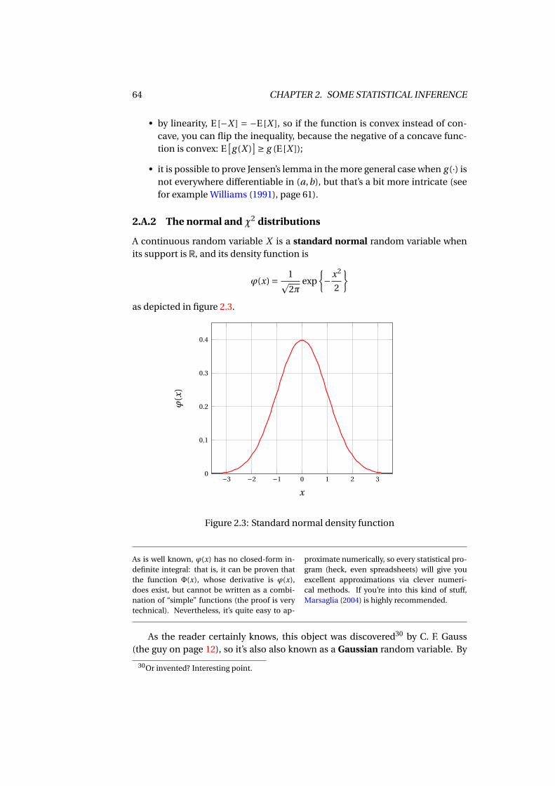
64 CHAPTER 2. SOME STATISTICAL INFERENCE
• by linearity, E[−X ] = −E[X ], so if the function is convex instead of con-cave, you can flip the inequality, because the negative of a concave func-tion is convex: E
[g (X )
]≥ g (E[X ]);
• it is possible to prove Jensen’s lemma in the more general case when g (·) isnot everywhere differentiable in (a,b), but that’s a bit more intricate (seefor example Williams (1991), page 61).
2.A.2 The normal and χ2 distributions
A continuous random variable X is a standard normal random variable whenits support is R, and its density function is
ϕ(x) = 1p2π
exp
−x2
2
as depicted in figure 2.3.
−3 −2 −1 0 1 2 30
0.1
0.2
0.3
0.4
x
ϕ(x
)
Figure 2.3: Standard normal density function
As is well known, ϕ(x) has no closed-form in-definite integral: that is, it can be proven thatthe function Φ(x), whose derivative is ϕ(x),does exist, but cannot be written as a combi-nation of “simple” functions (the proof is verytechnical). Nevertheless, it’s quite easy to ap-
proximate numerically, so every statistical pro-gram (heck, even spreadsheets) will give youexcellent approximations via clever numeri-cal methods. If you’re into this kind of stuff,Marsaglia (2004) is highly recommended.
As the reader certainly knows, this object was discovered30 by C. F. Gauss(the guy on page 12), so it’s also also known as a Gaussian random variable. By
30Or invented? Interesting point.
2.A. ASSORTED RESULTS 65
playing with integrals a little31, it can be proven that E[X ] = 0 and V[X ] = 1. Oneof the many nice properties of Gaussian rvs is that an affine transformation of anormal rv is also normal. Therefore, by the rules for expected values (see section2.2.3), if X is a standard normal rv, then Y = m + s · X is a normal rv with meanm and variance s2. Its density function is
f (y) = 1p2πs2
exp
− (y −m)2
2s2
A compact way to say this is Y ∼ N (m, s2).
In fact, one can define a multivariate normal random variable as a randomvector x with density
f (x) = (2π)−n/2|Σ|−1/2 exp(x−m)′Σ−1(x−m)
,
or, in short, x ∼ N (m,Σ), where n is the dimension of x, m is its expectation andΣ its covariance matrix. The multivariate version of this random variable alsoenjoys the linearity property, so if x ∼ N (m,Σ), then
y = Ax+b ∼ N (Am+b, AΣA′). (2.15)
It is easy to overlook how amazing this result is: the fact that E[Ax+b] =AE[x]+b is true for any distribution and does not depend on Gaussianity; andthe same holds for the parallel property of the variance. The special thing aboutthe Gaussian distribution is that a linear transformation of a Gaussian rv is itselfGaussian. And this is a very special property, that is only shared by a few distri-butions (for example: if you take a linear combination of two Bernoulli rvs, theresult is not Bernoulli-distributed).
The Gaussian distribution has a very convenient feature: contrary to whathappens in general, if X and Y have a joint normal distribution (that is, the vec-tor x = [Y , X ] is a bivariate normal rv), absence of correlation implies indepen-dence (again, this can be proven quite easily: nice exercise left to the reader).Together with the linearity property, this also implies another very importantresult: if y and x are jointly Gaussian, then the conditional density f (y|x) is Gaus-sian as well. In formulae:
f (y|x) = (2π)−n/2|Σ|−1/2 exp(y−m)′Σ−1(x−m)
,
where
m = E[y|x]= E
[y]+B ′ (x−E[x])
B = Σ−1x Σx,y
Σ = V[y|x]=Σy −Σ′
x,yΣ−1x Σx,y
where Σy is the covariance matrix of y, Σx is the covariance matrix of x and Σx,y
is the matrix of covariances between x and y.
31If you want to have some fun with the moments of the standard normal distribution, you’ll
find the resultdϕ(x)
dx =−xϕ(x) very useful, because it implies that∫
xϕ(x)dx =−ϕ(x).
66 CHAPTER 2. SOME STATISTICAL INFERENCE
Example 2.9For example, suppose that the joint distribution of y and x = [x1, x2] is normal,with
E
yx1
x2
= 1
23
V
yx1
x2
= 3 0 1
0 1 11 1 2
then you have
E[
y]= 1 E[x] = [2,3]′ Σy = 3 Σx =
[1 11 2
]Σx,y = [0,1]′
and therefore
B =[
1 11 2
]−1 [01
]=
[−11
]Σ = 3− [
0 1][
1 11 2
]−1 [01
]= 3−1 = 2,
since
[1 11 2
]−1
=[
2 −1−1 1
]. As a consequence, the conditional expectation of y
given x equals
E[y|x]= 1+ [−1,1]′
[x1 −2x3 −3
]=−x1 +x2
and in conclusiony |x ∼ N [x2 −x1,2] .
Note that:
• the conditional mean is a linear function of the x; this needn’t happen ingeneral: it’s a miraculous property of Gaussian random variables;
• the conditional variance is not a function of the x variables (it’s a con-stant); again, this doesn’t happen in general, but with Gaussian randomvariables, it does;
• if you apply the Law of Iterated Expectations (eq. (2.7)) you get
E[E
[y |x]]=−E[x1]+E[x2] =−2+3 = 1 = E
[y]
;
quelle surprise!
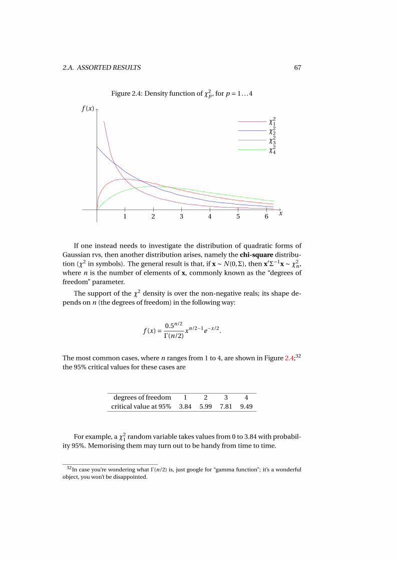
2.A. ASSORTED RESULTS 67
Figure 2.4: Density function of χ2p , for p = 1. . .4
x
f (x)
χ21χ2
2χ2
3χ2
4
1 2 3 4 5 6
If one instead needs to investigate the distribution of quadratic forms ofGaussian rvs, then another distribution arises, namely the chi-square distribu-tion (χ2 in symbols). The general result is that, if x ∼ N (0,Σ), then x′Σ−1x ∼ χ2
n ,where n is the number of elements of x, commonly known as the “degrees offreedom” parameter.
The support of the χ2 density is over the non-negative reals; its shape de-pends on n (the degrees of freedom) in the following way:
f (x) = 0.5n/2
Γ(n/2)xn/2−1e−x/2.
The most common cases, where n ranges from 1 to 4, are shown in Figure 2.4;32
the 95% critical values for these cases are
degrees of freedom 1 2 3 4critical value at 95% 3.84 5.99 7.81 9.49
For example, a χ21 random variable takes values from 0 to 3.84 with probabil-
ity 95%. Memorising them may turn out to be handy from time to time.
32In case you’re wondering what Γ(n/2) is, just google for “gamma function”; it’s a wonderfulobject, you won’t be disappointed.
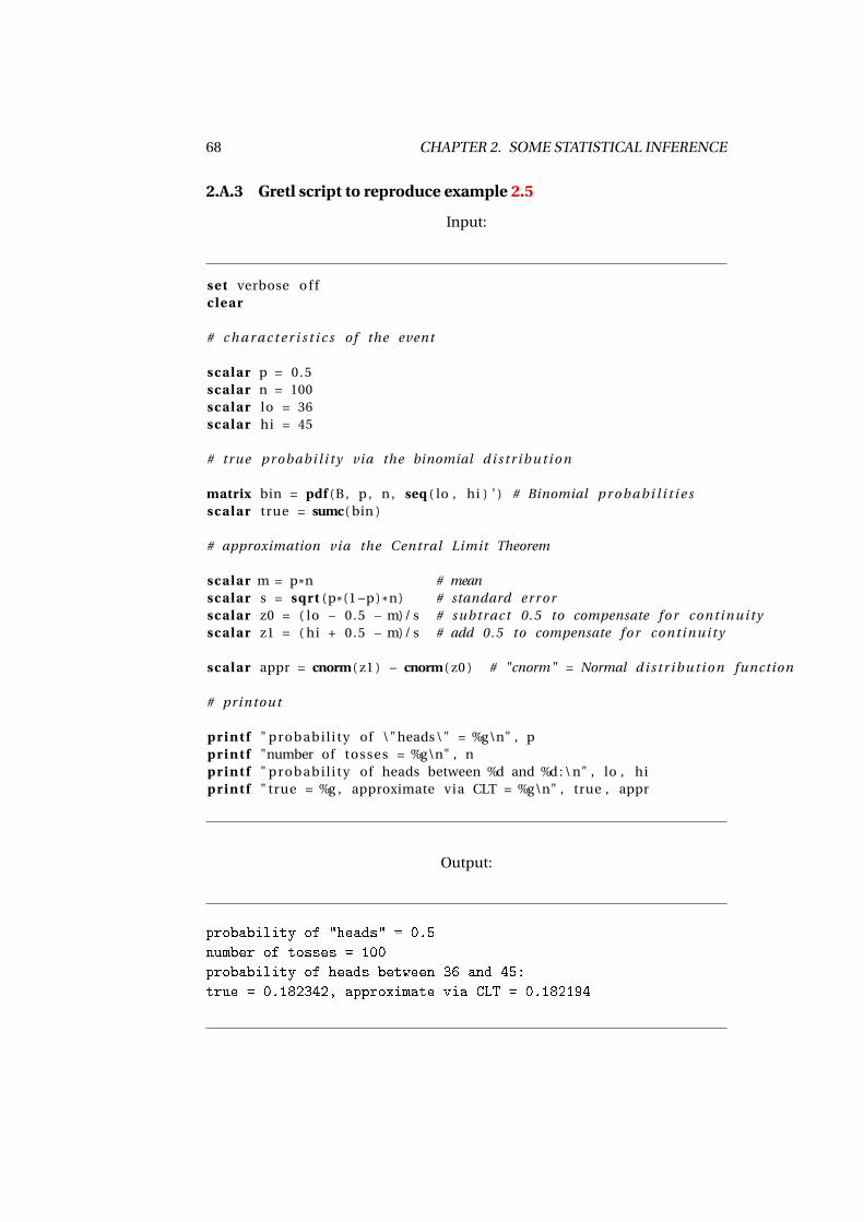
68 CHAPTER 2. SOME STATISTICAL INFERENCE
2.A.3 Gretl script to reproduce example 2.5
Input:
set verbose o f fclear
# c h a r a c t e r i s t i c s of the event
scalar p = 0.5scalar n = 100scalar lo = 36scalar hi = 45
# true p r ob a bi l i t y via the binomial d i s t r i b u t i o n
matrix bin = pdf (B, p , n , seq ( lo , hi ) ’ ) # Binomial p r o b a b i l i t i e sscalar true = sumc( bin )
# approximation via the Central Limit Theorem
scalar m = p*n # meanscalar s = sqrt (p*(1 −p) *n) # standard err orscalar z0 = ( lo − 0.5 − m)/ s # subtract 0.5 to compensate f o r continuityscalar z1 = ( hi + 0.5 − m)/ s # add 0.5 to compensate f o r continuity
scalar appr = cnorm( z1 ) − cnorm( z0 ) # "cnorm" = Normal d i s t r i b u t i o n function
# printout
printf " probabi l i ty of \"heads\" = %g\n" , pprintf "number of tosses = %g\n" , nprintf " probabi l i ty of heads between %d and %d : \ n" , lo , hiprintf " true = %g , approximate via CLT = %g\n" , true , appr
Output:
probability of "heads" = 0.5
number of tosses = 100
probability of heads between 36 and 45:
true = 0.182342, approximate via CLT = 0.182194
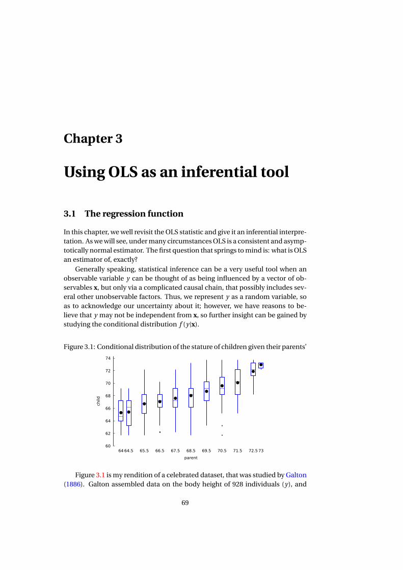
Chapter 3
Using OLS as an inferential tool
3.1 The regression function
In this chapter, we well revisit the OLS statistic and give it an inferential interpre-tation. As we will see, under many circumstances OLS is a consistent and asymp-totically normal estimator. The first question that springs to mind is: what is OLSan estimator of, exactly?
Generally speaking, statistical inference can be a very useful tool when anobservable variable y can be thought of as being influenced by a vector of ob-servables x, but only via a complicated causal chain, that possibly includes sev-eral other unobservable factors. Thus, we represent y as a random variable, soas to acknowledge our uncertainty about it; however, we have reasons to be-lieve that y may not be independent from x, so further insight can be gained bystudying the conditional distribution f (y |x).
Figure 3.1: Conditional distribution of the stature of children given their parents’
60
62
64
66
68
70
72
74
64 64.5 65.5 66.5 67.5 68.5 69.5 70.5 71.5 72.5 73
child
parent
Figure 3.1 is my rendition of a celebrated dataset, that was studied by Galton(1886). Galton assembled data on the body height of 928 individuals (y), and
69
70 CHAPTER 3. USING OLS AS AN INFERENTIAL TOOL
matched them against the average height of their parents (x). Data are in inches.
FRANCIS GALTON
It is natural to think that somebody’s stature is the re-sult of a multiplicity of causes, but surely the hereditarycomponent cannot be negligible. Therefore, the interestin f (y |x). For each observed value in of x in the sample,Figure 3.1 shows the corresponding boxplot.
Maybe not all readers are familiar with boxplots, so al-low me to explain how to read the “candlesticks” in the fig-ure: each vertical object consists of a central “box”, fromwhich two “whiskers” depart, upwards and downwards.The central box encloses the middle 50% of the data, i.e.it is bounded by the first and third quartiles. The “whiskers” extend from eachend of the box for a range equal at most to 1.5 times the interquartile range. Ob-servations outside that range are considered outliers1 and represented via dots.A line is drawn across the box at the median. Additionally, a black dot indicatesthe average.
The most notable feature of Figure 3.1 is that the boxes seem to go up to-gether with x; that is, the distribution of y shifts towards higher values as x grows.However, even considering the subset of observations defined as the childrenwhose parents were of a certain height, some dispersion remains. For example,if we focus on x = 65.5, you see from the third candlestick from the left that theminimum height is about 62 and the maximum is about 72, while the mean isbetween 66 and 68 (in fact, the precise figure is 67.059).
Historical curiosity: if you use OLS to gothrough those points such as to minimise theSSR, you will find that the fitted line is ci =23.9+0.646pi , where ci stands for “child” andpi for “parent”. The fact that the slope of thefitted line is less than 1 prompted Galton to ob-serve that the tendency for taller parents was to
have children who were taller than the average,but not as much as themselves (and of coursethe same, in reverse, happened to shorter par-ents). Galton described this state of things as“Regression towards Mediocrity”, and the termstuck.
This method of inquiry is certainly interesting, but also very demanding: ifx had been a vector of characteristics, rather than a simple scalar, the analysiswould have been too complex to undertake. However, we may focus on a morelimited problem, that is hopefully amenable to a neat and tidy solution.
Instead of studying f (y |x), we could focus on the conditional expectationE
[y |x]
: this object contains the information on how the centre of the distribu-tion of y varies across different values of x, and in most cases is just what wewant. If you join the dots in figure 3.1, you have an upward-sloping line, thatsuits very well our belief that taller parents should have, as a rule, taller children.
The next ingredient for making this intuition operational is to assume that
1An “outlier” is a data point that is far away from the rest.
3.1. THE REGRESSION FUNCTION 71
E[
y |x]is a simple function, whose shape is governed by a few parameters.2 The
choice that is nearly universally made is that of a linear3 function: E[
y |x]= x′β.Now define the random variable ε = y − x′β, so that y can be written (by def-inition) as x′β+ ε. If we observe multiple realisations of y and x, then we canwrite
yi = x′iβ+εi (3.1)
or, in matrix form,y = Xβ+ε (3.2)
For historical reasons, the random variable ε is called the disturbance; the ideahere is that if εi was 0, by observing yi we would observe E
[yi |xi
]in its “uncon-
taminated” form.
Like many other terms in use in economet-rics, the word comes from the statistical liter-ature that predated econometrics proper. Inother disciplines, mainly experimental ones, itis quite natural to think of the regression func-tion as a “Law of Nature” and of ε as some ran-dom fluctuation in our data, coming from ex-
perimental errors, bad measurement, and soon. These considerations make it quite natu-ral, in experimental science, to surmise that thedistribution of ε should be roughly normal, asa consequence of the CLT. Unfortunately, thisposition is untenable in economics.
A very important property of the random variable ε is that it’s orthogonal tox by construction:4
E[x ·ε] = 0 (3.3)
The proof is simple: since ε= y −x′β, clearly
E[ε|x] = E[
y |x]−E[x′β|x]= x′β−x′β = 0;
therefore, by the law of iterated expectations (see Section 2.2.4),
E[x ·ε] = E[x ·E[ε|x]] = E[x ·0] = 0.
Note the difference between equation (3.2) and the parallel OLS decompo-sition y = Xβ+e, where everything on the right-hand side of the equation is anobservable statistic. Instead, the only observable item in the right-hand side of(3.2) is X: β is an unobservable vector of parameters and ε is an unobservablevector of random variables. Still, the similarity is striking; it should be no sur-prise that, under appropriate conditions, β is a CAN estimator of β, which weprove in the next section.
2In fact, there are techniques for estimating the regression function directly, without resortingto assumptions on its functional form. These techniques are grouped under the term nonpara-metric regression. Their usage in econometrics is rather limited, however, chiefly because of theirgreater compuatational complexity and of the difficulty of computing marginal effects.
3As for what we mean exactly by “linear”, see 1.3.2.4Warning: as shown in the text, E[ε|x] = 0 =⇒ E[x ·ε] = 0, but the converse is not necessarily
true.
72 CHAPTER 3. USING OLS AS AN INFERENTIAL TOOL
3.2 Main statistical properties of OLS
A handy consequence of equation (3.2) is that the OLS statistic can be written as
β = (X′X)−1X′y =β+ (X′X)−1X′ε (3.4)
As any estimator, β has a distribution, and its finite-sample properties can bestudied, in some cases. For example, its unbiasedness is very easy to prove: ifE[ε|X] = 0, then
E[β|X]=β+E
[(X′X)−1X′ε|X]=β+ (X′X)−1X′E[ε|X] =β.
And therefore, by the law of iterated expectations,
E[β
]= E[E
[β|X]]= E
[β
]=β.
However, nobody cares about unbiasedness nowadays. Moreover, in orderto say something on the distribution of β we’d need assumptions on the distri-bution of ε, which is something we’d rather avoid doing. Therefore, we’ll useasymptotic results. Of course, we will assume that the data are such that limittheorems apply (iid being but an example).
3.2.1 Consistency
In order to prove consistency, start from equation (3.4) and rewrite matrix prod-ucts as sums:
β =β+[∑
ixi x′i
]−1 ∑i
xiεi =β+[
1
n
∑i
xi x′i
]−11
n
∑i
xiεi . (3.5)
Let’s analyse the two terms on the right-hand side separately: in order to do so,it will be convenient to define the vector
zi = xiεi ; (3.6)
given equation (3.3), E[z] = 0, so a straightforward application of the LLN gives
1
n
∑i
xiεip−→ 0. (3.7)
As for the limit of the first term, assume that n−1X′X has one, and call it Q:5
1
n
∑i
xi x′ip−→Q; (3.8)
5Ordinarily, Q will be equal to E(xi x′i ).
3.2. MAIN STATISTICAL PROPERTIES OF OLS 73
if Q is invertible, then we can exploit the fact that inversion is a continuous trans-formation as follows [
1
n
∑i
xi x′i
]−1p−→Q−1,
so, after putting the two pieces together,
βp−→β+Q−1 ·0 =β.
The OLS statistic, therefore, is a consistent estimator of the parameters ofthe conditional mean, or to be more technical, of the derivative of E
[y |x]
withrespect to x, which is constant by the linearity hypothesis.
One may think that the whole argument wouldbreak down if the assumption of linearity wereviolated. This is not completely true: even inmany cases when E
[y |x]
is non linear, it maybe proven that β is a consistent estimator of the
parameters of an object called Optimal LinearPredictor, which includes the linearity as a spe-cial case. But this is far too advanced for a booklike this.
It’s important here to ensure that 1n
∑i xi x′i converges to an invertible matrix;
this may not happen for two reasons:
1. it may not converge to any limit; this would be the case if, for example, thevector x possessed no second moments;6
2. it may converge to a singular matrix; this, for example, would happen incases such as xt =φt , where |φ| < 1.
However, in ordinary circumstances, such problems should not arise.
3.2.2 Asymptotic normality
From equation (3.5),
pn
(β−β)= [
1
n
∑i
xi x′i
]−11pn
∑i
xiεi
we already know from the previous subsection that[ 1
n
∑i xi x′i
]−1 p−→ Q−1, butwhat happens to the second term as n grows to infinity? Define zi as in equation(3.6). Therefore, by the CLT,
1pn
∑i
xiεi =p
n Zd−→ N [0,Ω],
6In fact, there are cases when this situation may be handled by using a scaling factor other thann−1; but let’s ignore such acrobatics.
74 CHAPTER 3. USING OLS AS AN INFERENTIAL TOOL
where Ω≡ V[zi ] = E[zi z′i
]. Therefore, we can use Cramér’s theorem (see (2.12))
as follows: since
pn
(β−β) =
[1
n
∑i
xi x′i
]−11pn
∑i
xiεi[1
n
∑i
xi x′i
]−1p−→ Q−1
1pn
∑i
xiεid−→ N [0,Ω]
the quantityp
n(β−β)
converges to a normal rv multiplied by the nonstochas-tic matrix Q−1; therefore, the linearity property for Gaussian rvs applies (see eq.(2.15)), and as a consequence
pn
(β−β) d−→ N
[0,Q−1ΩQ−1] . (3.9)
In order to say something on Ω, we can use the law of iterated expectations(see section 2.2.4) to re-write it as follows:
Ω= E[zi z′i
]= E[ε2
i ·xi x′i]= E
[E
[ε2
i |xi] ·xi x′i
].
The quantity E[ε2
i |xi]
is a bit of a problem here. We proved quite easily thatE[ε|x] = 0 as a natural consequence of the way ε is defined (see section 3.1,near the end). However, we know nothing about its second conditional moment(more succinctly definable as the conditional variance of y , if you like). For allwe know, it may even not exist; or if it does, it could be an arbitrary (and possiblyquite weird) function of x.
In the present chapter, we will assume that E[ε2|x]
is a positive constant,traditionally labelled σ2:
E[ε2|x]=σ2; (3.10)
the most important implication of this assumption is that the conditional vari-ance V
[yi |xi
]is constant for all observations i = 1. . .n; this idea is known as
homoskedasticity. Therefore, under the homoskedasticity assumption,
Ω= E[zi z′i
]= E[σ2 ·xi x′i
]=σ2 ·E[xi x′i
]=σ2Q
and equation (3.9) simplifies to
pn
(β−β) d−→ N
[0,σ2Q−1] . (3.11)
This result is also important because it provides the basis for justifying the usageof OLS as an estimator of β on the grounds of its efficiency. Traditionally, this isproven via the so-called Gauss-Markov theorem, which, however, relies quite
3.3. SPECIFICATION TESTING 75
heavily on small-sample results that I don’t like very much.7 In fact, there isa much more satisfactory proof that OLS is asymptotically semiparametricallyefficient, but it’s considerably technical, so it’s way out of scope here.8 Suffice itto say that, under homoskedasticity, OLS is hard to beat in terms of efficiency.
We can estimate consistently Q via n−1X′X and σ2 via9
σ2 = e′en
p−→σ2 (3.12)
so the approximate distribution for OLS that we use is
βa∼ N
[β,V
]where V = σ2(X′X)−1.
A word of warning: the expression above V is not the one used by the major-ity of econometrics textbooks, and by none of the major econometric softwarepackages. Instead, most people usually prefer a variant in which an alternativeestimator of σ2 is used:
s2 = e′en −k
,
where k is the number of elements of β; the number n −k is commonly knownas degrees of freedom. It’s easy to prove that s2 is also consistent, but (as can beproven via some neat algebra trick that I’m sparing you here) it’s also unbiased:E
[s2
]=σ2.The difference between the two variants is negligible for any reasonable sam-
ple size n, so you can use either; or to put it otherwise, if using s2 instead of σ2
makes a substantial difference, then n is probably so small that in my opinionyou shouldn’t be using statistical inference in the first place. And besides, I seeno convincing reason why unbiasedness should be considered a virtue in thiscontext. The usage of σ2, instead, makes many things easier and is consistentwith all the rest of procedures that econometricians use beyond OLS, in whichasymptotic results are uniformly used. Having said this, let’s move on.
3.3 Specification testing
3.3.1 Tests on a single coefficients
Sometimes, we would like to test hypotheses on elements of β, so that we candecide optimally on which explanatory variables we must include in our regres-sion function. This is often called “specification testing”.
7If you really really care, a proof is given in section 3.A.2, but I don’t care about it very muchmyself.
8See Hansen (2019), sections 7.20 and 7.21 if you’re interested.9Proof of this is unnecessary, but if you insist, go to subsection 3.A.1.
76 CHAPTER 3. USING OLS AS AN INFERENTIAL TOOL
Let’s begin by testing a very simple hypothesis: H0 : βi = 0. The practicalimplication of H0 in a model like
E[
y |x]= x1β1 +x2β2 +·· ·+xkβk =k∑
j=1x jβ j
is that the impact of xi on E[
y |x]is 0, and therefore that the i -th explanatory
variable is irrelevant, since it has no effect on the regression function.Note that under H0 there are two equally valid representations of the regres-
sion function; one that includes xi , the other one that doesn’t. For example, fori = 2 and k = 3,
Model A yi = x1iβ1 +x2iβ2 +x3iβ3 +εi (3.13)
Model B yi = x1iβ1 +x3iβ3 +εi (3.14)
Clearly, if H0 was true, model B would be preferable, chiefly on the grounds ofparsimony;10 however, if H0 was false, only model A would be a valid represen-tation of the regression function.
As I explained in section 2.4, in order to test H0 we need to find a differen-tiable function of β such that g (β) = 0 if and only if H0 is true. In this case, thisis very easy: define ui the i -th column of the identity matrix (aka “extractionvector”); equivalently, we may say that ui is a vector of zeros, except for the i -thelement, which is 1.11 The extraction vector takes its name by the fact that theinner product of u j by any vector a returns the j -element of a. For example, theproduct A ·u2 yields the second column of A, while u′
2 A yields its second row.12
Evidently, u′i Au j = Ai j .
By defining g (β) = u′iβ, the hypothesis H0 : βi = 0 can be written as H0 :
u′iβ = 0, and the Jacobian term is simply u′
i . Hence
pn
[u′
i β−u′iβ
] d−→ N[0,u′
i V ui]
so our test statistic is
β′ui(u′
i V ui)−1
u′i β = β2
i
vi i= t 2
i (3.15)
where ti = βi
sei, vi i is the i -th element on the diagonal of V and sei =p
vi i . The
quantity sei is usually referred to as the standard error of βi .In fact, it’s rather easy to prove that we could use a slight generalisation of
the above for constructing a test for H0 : βi = a, where a is any real number youwant, and that such a test takes the form
tβi=a = βi −a
sei(3.16)
10In fact, we will argue in section 3.6 that OLS on model B would produce a more efficient esti-mator.
11The reader may recall that I used the u vector in a different context, in section 1.5.12As always, the reader should verify the claim, instead of trusting me blindly.
3.3. SPECIFICATION TESTING 77
Clearly, we can use the t statistic to decide whether a certain explanatory vari-able is irrelevant or not, and therefore choose between model A and model B. Inthe next subsection, I will show how this idea can be nicely generalised so as toframe the decision on the best specification via hypothesis testing.
3.3.2 More general tests
The general idea I will pursue here can be stated as follows: we assume we havea true representation of the conditional mean, that I will call the unrestrictedmodel; in the previous subsection, that was called “model A”. Additionally, weconjecture that the parameters β may obey some restrictions (also known asconstraints); by incorporating those into our unrestricted model, we would ob-tain a more compact representation of the regression function. This, however,would be valid only if our conjecture was true. This model is known as the re-stricted model, and was labelled “model B” in the previous subsection. We makeour decision on the model to adopt by testing if our conjecture via a standard hy-pothesis test.
In order to exemplify this idea, I will use the following unrestricted model:
E[
yi |xi]= x1iβ1 +x2iβ2 +x3iβ3 (3.17)
in the previous subsection, we saw the the restricted model corresponding tothe constraint β2 = 0 is
E[
yi |xi]= x1iβ1 +x3iβ3.
Suppose now that instead of β2 = 0, our conjecture was β1 = 1; the restrictedversion of (3.17) would become
E[
yi −x1i |xi]= x2iβ2 +x3iβ3,
and we would be in fact studying the regression function of the observable vari-able yi = yi − x1i on x2i and x3i . Note that in this case we would redefine thedependent variable of our model.
One more example: suppose we combine (3.17) with the restrictionβ2+β3 =0 (or, equivalently, β2 =−β3): in this case, the constrained model turns out to be
E[
yi |xi]= x1iβ1 + (x2i −x3i )β2.
Of course you can combine more than one restriction into a system:β1 = 1β2 +β3 = 0,
and if you applied these to (3.17), the constrained model would turn into
E[
yi −x1i |xi]= (x2i −x3i )β2.
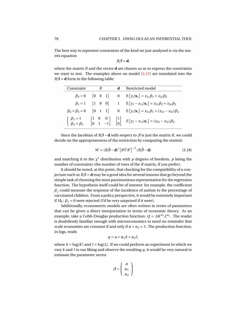
78 CHAPTER 3. USING OLS AS AN INFERENTIAL TOOL
The best way to represent constraints of the kind we just analysed is via the ma-trix equation
Rβ = d,
where the matrix R and the vector d are chosen so as to express the constraintswe want to test. The examples above on model (3.17) are translated into theRβ = d form in the following table:
Constraint R d Restricted model
β3 = 0[0 0 1
]0 E
[yi |xi
]= x1iβ1 +x2iβ2
β1 = 1[1 0 0
]1 E
[yi −x1i |xi
]= x2iβ2 +x3iβ3
β2 +β3 = 0[0 1 1
]0 E
[yi |xi
]= x1iβ1 + (x2i −x3i )β2β1 = 1β2 =β3
[1 0 00 1 −1
] [10
]E
[yi −x1i |xi
]= (x2i −x3i )β2
Since the Jacobian of Rβ−d with respect to β is just the matrix R, we coulddecide on the appropriateness of the restriction by computing the statistic
W = (Rβ−d)′[RV R ′]−1
(Rβ−d) (3.18)
and matching it to the χ2 distribution with p degrees of freedom, p being thenumber of constraints (the number of rows of the R matrix, if you prefer).
It should be noted, at this point, that checking for the compatibility of a con-jecture such as Rβ = d may be a good idea for several reasons that go beyond thesimple task of choosing the most parsimonious representation for the regressionfunction. The hypothesis itself could be of interest: for example, the coefficientβ j could measure the response of the incidence of autism to the percentage ofvaccinated children. From a policy perspective, it would be extremely importantif H0 :β j = 0 were rejected (I’d be very surprised if it were).
Additionally, econometric models are often written in terms of parametersthat can be given a direct interpretation in terms of economic theory. As anexample, take a Cobb-Douglas production function: Q = AKα1 Lα2 . The readeris doubtlessly familiar enough with microeconomics to need no reminder thatscale economies are constant if and only if α+α2 = 1. The production function,in logs, reads
q = a +α1k +α2l ,
where k = log(K ) and l = log(L). If we could perform an experiment in which wevary k and l to our liking and observe the resulting q , it would be very natural toestimate the parameter vector
β = aα1
α2
3.4. EXAMPLE: READING THE OUTPUT OF A SOFTWARE PACKAGE 79
by means of an OLS regression, and the hypothesis “constant returns to scale”would simply amount to Rβ = d, with
R = [0 1 1] d = 1.
Nevertheless, if we knew for certain (by some supernatural revelation) thatour production function displays in fact constant returns to scale, we would likeour estimate of β to incorporate the information α1 +α2 = 1, and there is noreason why β should.
In section 3.6, we will develop an alternative estimator, known as the Re-stricted Least Squares estimator (or RLS for short), which integrates sampledata with one or more a priori constraints on the parameter vector. As we willsee, this will have the additional advantage of providing us with to calculate theW test statistic, by comparing the SSRs for the two versions of the model.
3.4 Example: reading the output of a software package
Now it’s time for a hands-on example:13 Table 3.1 contains a regression on adataset containing data about 2610 home sales in Stockton, CA from Oct 1, 1996to Nov 30, 1998;14 the dependent variable is the natural logarithm of their saleprice. For this example, the software package I used is gretl, but the output ismore or less the same with every other program.
The model we’re going to estimate can be written as follows:
pi =β0 +β1si +β2bi +β3ai +β4xi +εi (3.19)
where pi is the log price of the i -th house and the explanatory variables are:
Legendlsize si log of living area, hundreds of square feetbaths bi number of bathsage ai age of home at time of sale, years
pool xi = 1 if home has pool, 0 otherwise
Models of this type, where the dependent variable is the price of a good andthe explanatory variables are its features, are commonly called hedonic models.In this case (like in most hedonic models), the dependent variable is in loga-rithm; therefore, the effect of all coefficients must be interpreted as the impacton that variable on the relative change in the house price (see footnote 29 inChapter 1).
13After reading this section, the reader might want to go back to section 1.6 and read it againfrom a different perspective.
14Data are taken from Hill et al. (2018); if you use gretl, you can find the data in gdt formatat http://www.learneconometrics.com/gretl/poe5/data/stockton5.gdt. This is part ofthe rich offering you find on Lee Adkins’ excellent website http://www.learneconometrics.
com/gretl/, which also contains Lee’s book. Highly recommended.
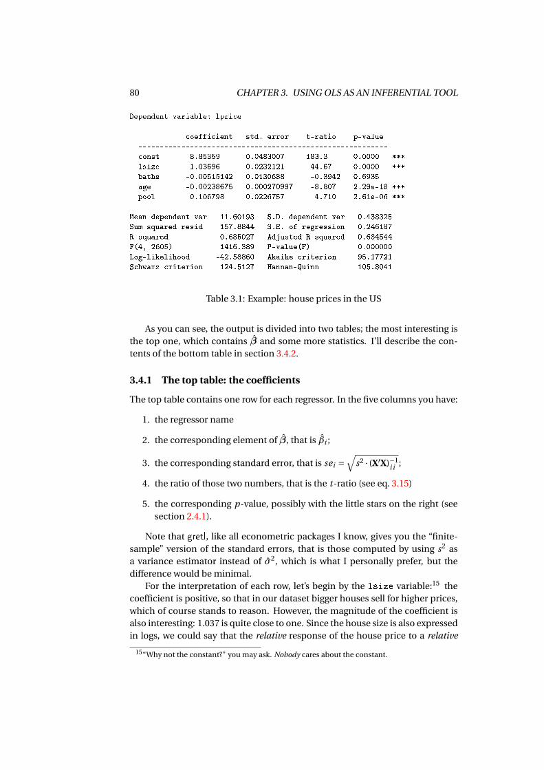
80 CHAPTER 3. USING OLS AS AN INFERENTIAL TOOL
Dependent variable: lprice
coefficient std. error t-ratio p-value
----------------------------------------------------------
const 8.85359 0.0483007 183.3 0.0000 ***
lsize 1.03696 0.0232121 44.67 0.0000 ***
baths -0.00515142 0.0130688 -0.3942 0.6935
age -0.00238675 0.000270997 -8.807 2.29e-18 ***
pool 0.106793 0.0226757 4.710 2.61e-06 ***
Mean dependent var 11.60193 S.D. dependent var 0.438325
Sum squared resid 157.8844 S.E. of regression 0.246187
R-squared 0.685027 Adjusted R-squared 0.684544
F(4, 2605) 1416.389 P-value(F) 0.000000
Log-likelihood -42.58860 Akaike criterion 95.17721
Schwarz criterion 124.5127 Hannan-Quinn 105.8041
Table 3.1: Example: house prices in the US
As you can see, the output is divided into two tables; the most interesting isthe top one, which contains β and some more statistics. I’ll describe the con-tents of the bottom table in section 3.4.2.
3.4.1 The top table: the coefficients
The top table contains one row for each regressor. In the five columns you have:
1. the regressor name
2. the corresponding element of β, that is βi ;
3. the corresponding standard error, that is sei =√
s2 · (X′X)−1i i ;
4. the ratio of those two numbers, that is the t-ratio (see eq. 3.15)
5. the corresponding p-value, possibly with the little stars on the right (seesection 2.4.1).
Note that gretl, like all econometric packages I know, gives you the “finite-sample” version of the standard errors, that is those computed by using s2 asa variance estimator instead of σ2, which is what I personally prefer, but thedifference would be minimal.
For the interpretation of each row, let’s begin by the lsize variable:15 thecoefficient is positive, so that in our dataset bigger houses sell for higher prices,which of course stands to reason. However, the magnitude of the coefficient isalso interesting: 1.037 is quite close to one. Since the house size is also expressedin logs, we could say that the relative response of the house price to a relative
15“Why not the constant?” you may ask. Nobody cares about the constant.
3.4. EXAMPLE: READING THE OUTPUT OF A SOFTWARE PACKAGE 81
variation in the house size is 1.037. For example, if we compared two houseswhere house A is bigger than house B by 10% (and all other characteristics werethe same), we would expect the value of house A to be 10.37% higher than thatof house B.
As the reader knows, this is what in economics we call an elasticity: for acontinuous function you have that
η= dy
dx· x
y= dlog y
dlog x
because dlog ydy = 1
y and therefore dlog y = dyy . So, every time you see something
like log(y) = a +b log(x), you can safely interpret b as the elasticity of y to x.From an economic point of view, therefore, we would say that the elasticity
of the house price to its size is about 1. What is more interesting, the standarderror for that coefficient is about 0.023, which gives a t-ratio of 44.67, and thecorresponding p-value is such an infinitesimal number that the software justgives you 0.16 If we conjectured that there was no effect of size on price, thathypothesis would be strongly rejected on the grounds of empirical evidence. Inthe jargon of applied economists, we would say that size is significant (in thiscase, very significant).
If, instead, we wanted to test the more meaningful hypotheses H0 :β1 = 1, itwould be quite easy to compute the appropriate t statistic as per equation (3.16):
t = β1 −1
se1= 1.03696−1
0.0232121= 1.592
and the corresponding p-value would be about 11.1%, so we wouldn’t reject H0.On the other hand, we get a slightly negative effect for the number of baths
(−0.00515142). At first sight, this does not make much sense, since you wouldexpect that the more baths you have in the house, the more valuable your prop-erty is. How come we observe a negative effect?
There are two answers to this question: first, the p-value associated to thecoefficient is 0.6935, which is way over the customary 0.05 level. In other words,an applied economist would say that the baths variable is not significant. Thisdoes not mean that we can conclusively deduce that there is no effect. It meansthat, if there is one, it’s too weak for us to detect (and, for all we know, it might aswell be positive instead, albeit quite limited). Moreover, this is the effect of thenumber of baths other things being equal, as we know from the Frisch-Waughtheorem (see section 1.5). In this light, the result is perhaps less surprising: whyshould the number of baths matter, given the size of the house? Actually, a smallhouse filled with baths wouldn’t seem such a great idea, at least to me.
On the contrary, the two variables age and pool are highly significant. Thecoefficient for age, for example, is about -0.002: each year of age decreases the
16In case you’re curious: I can’t compute the number exactly, but it’s smaller than 10−310.
82 CHAPTER 3. USING OLS AS AN INFERENTIAL TOOL
house value by about 0.2%, which makes sense; the coefficient for the dummyvariable pool is about 0.107; therefore, it would seem that having a pool in-creases the house value by a little over 10%, which makes sense, again.
3.4.2 The bottom table: other statistics
Let’s begin with the easy bits; the first line of the bottom table contains descrip-tive statistics for the dependent variable: mean (about 11.6) and standard de-viation (about 0.43). The next line contains the sum of squared residuals e′e(157.88) and the square root of s2 = e′e/(n−k), which is in this case about 0.246.Since our dependent variable is in logs, this means that the “typical” size of theapproximation errors for our model is roughly 25%. The line below contains theR2 index and its adjusted variant (see eq. 1.19). Both versions are around 68.5%,which means that our model, all in all, does a fair job at describing price dif-ferentials between houses, given how little information on each properties wehave. However, our estimate of σ2 is quite sizeable, so we shouldn’t expect ourmodel to give us a detailed description of individual house prices.
The line below contains a test17 commonly called “overall specification test”:it is a joint test for all coefficient being zero apart from the constant. The nullhypothesis is, basically, that none of your regressors make any sense and yourmodel is utter rubbish. Luckily, in our case the p-value is infinitesimal, so wereject.
On the next line, you get the log-likelihood for the model:
L =−n
2
[1+ ln(2π)+ ln(σ2)
].
This number is of very little use by itself;18 in this book, it’s only important be-cause it provides the essential ingredient for calculating the so-called Informa-tion Criteria (IC), that are widely used tools for comparing non-nested models.
We say that a model nests another one when the latter is a special case ofthe former. For example, the two models (3.13) and (3.14) are nested, becausemodel (3.14) is just model (3.13) in the special case β2 = 0. If model B is nestedin model A, choosing between A and B is rather easy: all you need is a propertest statistic; I will provide a detailed exposition in Section 3.6. However, we mayhave to choose between the two alternatives in which nesting is impossible:
yi ' x′iβyi ' z′iγ
17This test, technically, is of the F variety — see section 3.6.1 for its definition.18If the data are iid and f (y |x) is Gaussian, then β and σ2 are the maximum likelihood estima-
tors ofβ andσ2. I chose not to include this topic into this book, but the interested reader will finda nice and compact exposition in Verbeek (2017), chapter 6. Other excellent treatments abound,but the curious reader may want to check out chapters 14–15 of Ruud (2000). If you want to go forthe real thing, grab Gourieroux and Monfort (1995), volume 1, chapter 7.
3.5. EXOGENEITY AND CAUSAL EFFECTS 83
Information criteria start from the value of the log-likelihood (multiplied by -2)and add a penalty function, which is increasing in the number of parameters.The gretl package, that I’m using here, reports three criteria: the Akaike IC (AIC),the Schwartz IC (BIC, where B is for “Bayesian”) and the one by Hannan andQuinn (HQC), which differ by the choice of penalty function:
AIC = −2L+2k (3.20)
BIC = −2L+k logn (3.21)
HQC = −2L+2k loglogn (3.22)
The rule is to pick the model that minimises information criteria. At times, itmay happen that this algorithm gives conflicting results depending on which ICyou choose. There is a huge literature on this, but my advice in these cases is“don’t trust the AIC much”. 19
3.5 Exogeneity and causal effects
This section is short, but very important. It is not about the statistical propertiesof β, but rather on its interpretation as an estimator of β, so it fits in well at thispoint of the book, although the point we pursue here will be discussed in muchgreater detail in Chapter 6.
What does βmeasure? If E[
y |x]= x′β, then β is simply defined as
β = ∂E[
y |x]∂x
;
therefore, in a wage equation, the coefficient for education tells us simply byhow much, on average, wage varies across different education levels.
It would be tempting to say “by how much your wage would change if yougot one extra year of education”, but unfortunately this statement would be un-warranted.20 There are many reasons why the conditional mean may not be agood indicator of causality: for example, people may just stop attending school,or university, the moment they are able to earn a decent wage. If that were thecase, the regression function of wage with respect to education would be flat, ifnot negative (because the smartest people would spend a shorter time in edu-cation). But this wouldn’t mean that education has a negative effect on wages.In fact, quite the contrary: people who get more education would do so to com-pensate for their lesser ability. Of course, this example is a bit of a stretch, but
19If you want some more detail on this, have a look at section 15.4 in Davidson and MacKin-non (2004) or section 3.2.2 in Verbeek (2017). However, the literature on statistical methods forselecting the “best” model (whatever that may mean) is truly massive; see for example the “modelselection” entry in (Durlauf and Blume, 2008).
20The ongoing debate in contemporary econometrics on the issue of differentiating betweencorrelation and causation is truly massive. For a quick account, read chapter 3 in the latest best-seller in econometrics, that is Angrist and Pischke (2008), or simply google for “Exogeneity”.
84 CHAPTER 3. USING OLS AS AN INFERENTIAL TOOL
should give you a hint as to why inferring causality from a regression coefficientmay be a very bad idea.
More in general, there are situations when the causal relationship betweeny and x works in such a way that the conditional mean does not capture causal-ity, but only the outcome of the process, which can be quite different, as in theexample I just made.
In these cases, the traditional phrase that we use in the economics commu-nity is “x is endogenous” (as opposed to exogenous). If regressors are endoge-nous, then the regression parameters have nothing to do with causal effects;put another way, the parameters of interest β are not those that describe theconditional mean, and therefore, if you define εi as yi − x′iβ, the first conse-quence is that the property E[εi |xi ] = 0 doesn’t hold anymore, and so E[εi xi ] =Cov[εi ,xi ] 6= 0. This is why in many cursory treatment of the subject, endo-geneity is described as an “illness” that happens when the regressors are cor-related with the disturbance term. Of course, that is an oversimplification: amore rigourous statement would be that in some cases the causal effects canbe different from the conditional mean; if you define the disturbances as de-viations from the causal effects, non-zero correlation between regressors anddisturbances follows by construction.
Note that this problem is not a shortcoming of OLS per se: the job of OLS is
to estimate consistently the parameters of the conditional expectation∂E[y |x]∂x . If
the nature of the problem is such that our parameters of interestβ are a differentobject and we insist on equating them with what OLS returns (thereby givingOLS a misleading interpretation), it’s a hermeneutical problem, not a statisticalone.
The preferred tool in the econometric tradition for estimating causal effectsis an estimator called Instrumental Variable estimator (or IV for short), butyou’ll have to wait until chapter 6 for it.
3.6 Restricted Least Squares and hypothesis testing
The Restricted Least Squares statistic (or RLS for short) is an estimator of theparameter vector that, like OLS, uses the available data in the most effective waybut at the same time, unlike OLS, satisfies by construction a set of p restrictionsof the type Rβ = d. In other words, we are looking for a vector β that minimisesthe SSR under the condition that a certain set of linear constraints are satisfied:
β = ArgminRβ=d
‖y−Xβ‖; (3.23)
compare (3.23) with equation (1.14): OLS is defined as the unconstrained SSRminimiser (we can choose β among all k-element vectors); RLS, instead, canonly be chosen among those vectorsβ that satisfy Rβ = d. Figure 3.2 exemplifiesthe situation for k = 2.
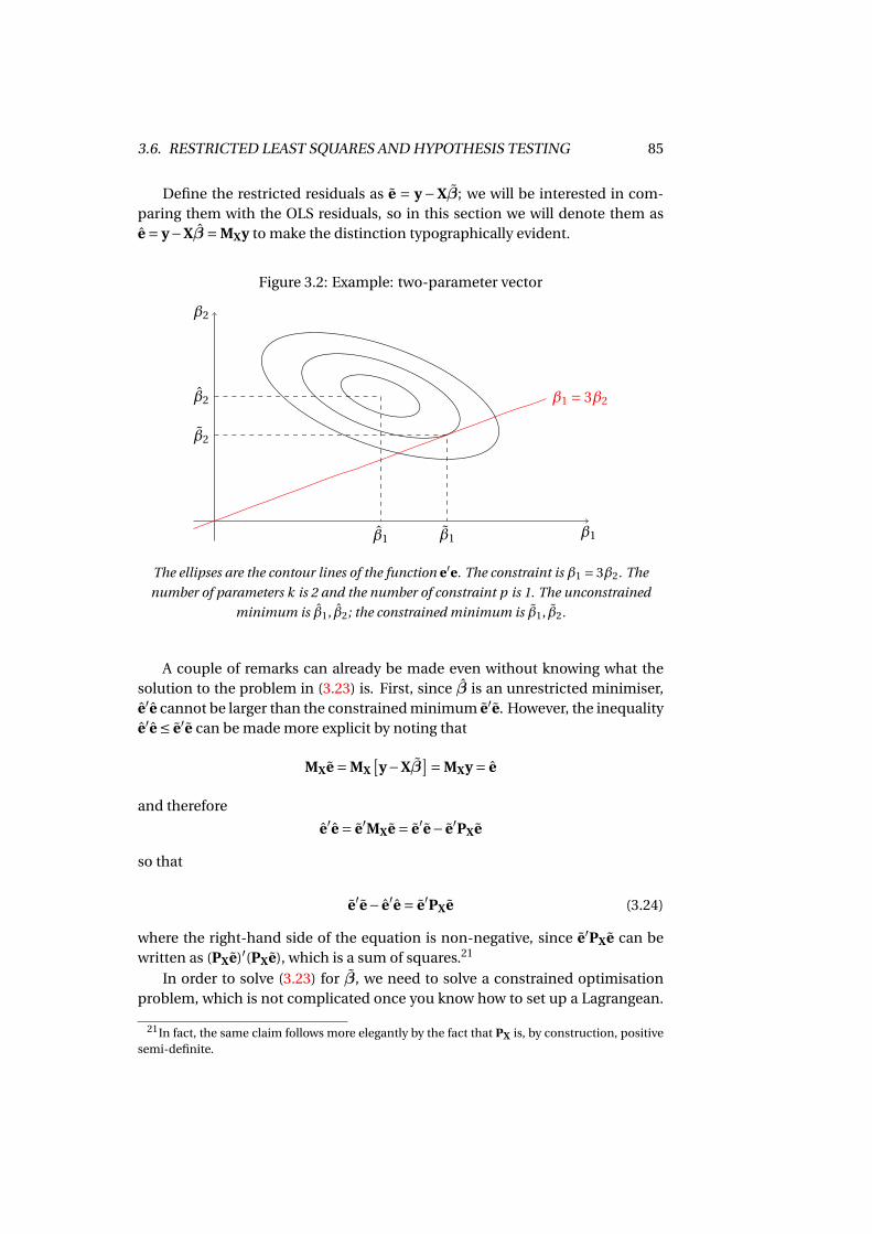
3.6. RESTRICTED LEAST SQUARES AND HYPOTHESIS TESTING 85
Define the restricted residuals as e = y−Xβ; we will be interested in com-paring them with the OLS residuals, so in this section we will denote them ase = y−Xβ = MXy to make the distinction typographically evident.
Figure 3.2: Example: two-parameter vector
β2
β1
β2
β1
β1 = 3β2
β2
β1
The ellipses are the contour lines of the function e′e. The constraint is β1 = 3β2. The
number of parameters k is 2 and the number of constraint p is 1. The unconstrained
minimum is β1, β2; the constrained minimum is β1, β2.
A couple of remarks can already be made even without knowing what thesolution to the problem in (3.23) is. First, since β is an unrestricted minimiser,e′e cannot be larger than the constrained minimum e′e. However, the inequalitye′e ≤ e′e can be made more explicit by noting that
MXe = MX[y−Xβ
]= MXy = e
and therefore
e′e = e′MXe = e′e− e′PXe
so that
e′e− e′e = e′PXe (3.24)
where the right-hand side of the equation is non-negative, since e′PXe can bewritten as (PXe)′(PXe), which is a sum of squares.21
In order to solve (3.23) for β, we need to solve a constrained optimisationproblem, which is not complicated once you know how to set up a Lagrangean.
21In fact, the same claim follows more elegantly by the fact that PX is, by construction, positivesemi-definite.
86 CHAPTER 3. USING OLS AS AN INFERENTIAL TOOL
The details, however, are not important here and I’ll give you the solution straightaway:
β = β− (X′X)−1R ′ [R(X′X)−1R ′]−1(Rβ−d); (3.25)
derivation of this result is provided in the separate subsection 3.A.3, so you canskip it if you want.
The statistical properties of β are proven in section 3.A.4, but the most im-portant point to make here are: if Rβ = d, then β is consistent just like the OLSestimator β, but has the additional advantage of being more efficient. If, on thecontrary, Rβ 6= d, then β is inconsistent. The practical consequence of this factis that, if we were certain that the equation Rβ = d holds, we would be muchbetter off by using an estimator that incorporates this information; but if ourconjecture is wrong, our inference would be invalid.
It’s also worth noting that nobody uses expression (3.25) as a computationaldevice. The simplest way to compute β is to run OLS on the restricted model andthen “undo” the restrictions: for example, if you take model (3.17), reproducedhere for your convenience
yi = x1iβ1 +x2iβ2 +x3iβ3 +εi
and want to impose the set of restrictions β1 = 1 and β2 = β3, what you woulddo is estimating the constrained version
yi −x1i = (x2i +x3i )β2 +εi , (3.26)
that can be “unravelled” as
yi = x1i ·1+x2iβ2 +x3iβ2 +εi
and then forming β as [1, β2, β2], where β2 is the OLS estimate of equation (3.26).Nevertheless, equation (3.25) is useful for proving an important result. Let’s
define the vector λ as
λ= [R(X′X)−1R ′]−1
(Rβ−d);
by premultiplying (3.25) by X we get:
Xβ = y = y−X(X′X)−1R ′λ
which in turn impliese = e+X(X′X)−1R ′λ
By using e = MXy =⇒ e′X = 0, we can use the above equation to get
e′e = e′e+λ′R(X′X)−1R ′λ
but by the definition of λ,
λ′R(X′X)−1R ′λ= (Rβ−d)′[R(X′X)−1R ′]−1
(Rβ−d)
3.6. RESTRICTED LEAST SQUARES AND HYPOTHESIS TESTING 87
so finally
e′e− e′e = (Rβ−d)′[R(X′X)−1R ′]−1
(Rβ−d). (3.27)
Note that the right-hand side of equation (3.27) is very similar to (3.18). Infact, if our estimator forσ2 is σ2 = e′e/n, we can combine equations (3.18), (3.24)and (3.27) to write the W statistic as:
W = (Rβ−d)′[R(X′X)−1R ′]−1
(Rβ−d)
σ2 = ne′e− e′e
e′e. (3.28)
Therefore, we can compute the same number in two different ways: one im-plies a rather boring sequence of matrix operations, using only ingredients thatare available after the estimation of the unrestricted model. The other one, in-stead, requires estimating both models, but at that point 3 scalars (the SSRs andthe number of observations) are sufficient for computing W .
3.6.1 Two alternative test statistics
There are two other statistics that can be used to perform a test on H0 instead ofthe W test. One is the so-called F test, which is the traditional statistic taught inall elementary econometric courses, treated with reverence in all introductoryeconometrics books and the one that all software packages report. It can bewritten as
F = e′e− e′es2
1
p= e′e− e′e
e′e· n −k
p; (3.29)
it can be easily seen that there are two differences between F and W : F usess2, the unbiased estimator of σ2 that I showed you at the end of section 3.2.2,instead of σ2; moreover, you also have the number of restrictions p in the de-nominator. Of course, it’s easy to compute them from one another:
W = p ·Fn
n −k⇐⇒ F = n −k
n(W /p)
so in the standard case, when n is much larger than k, you have that W ' p ·F .Since their p-values are always practically the same, there is no statistical groundfor preferring either. The reason why the econometricians of yore were attachedto the F test was because its distribution is known even for small samples if εi isnormal, so you don’t need asymptotics. In my opinion, however, small samplesare something you should steer clear of anyway, and postulating normality of εi
is, as a rule, just wishful thinking. So, my advice is: use W .The other statistic we can use is more interesting: if H0 is true, the restricted
model is just as correct as the unrestricted one. Therefore, one could conceiv-ably estimate σ2 by using e instead of e:
σ2 = e′en
(3.30)
88 CHAPTER 3. USING OLS AS AN INFERENTIAL TOOL
It can be proven that intuition is right, and if H0 is true σ2 is indeed consistentfor σ2. If we use σ2 instead of σ2 in equation (3.28), we obtain the so-called LMstatistic:22
LM = ne′e− e′e
e′e= n
e′PXe
e′e, (3.31)
where equality comes from (3.24). Since e′e cannot be less than e′e, in finitesamples LM will always be smaller than W . However, under H0 they tend to thesame probability limit, and therefore under the null LM will also by asymptoti-cally distributed as χ2
p .23
The nice feature of the LM statistic is that it can be computed via a neat trick,known as auxiliary regression:
1. run OLS on the constrained model and compute the residuals e;
2. run OLS on a model where the dependent variable is e and the regressorsare the same as in the unconstrained model;
3. take R2 from this regression and multiply it by n. What you get is the LMstatistic.
The last step is motivated by the fact that you can write R2 as y′PXyy′y , so in the
present case e′PXee′e is R2 from the auxiliary regression.
Example 3.1As an example, let’s go back to the house pricing model we used as an examplein Section 3.4. In Section 3.4.1 we already discussed two hypotheses of interest,namely:
• The price elasticity is 1, and
• the number of baths has no effect.
Testing for these two hypotheses separately is easy, via t-tests, which is just whatwe did a few pages back. As for the joint hypothesis, the easiest thing to do issetting up the resticted model as follows: combine equation (3.19) with β1 = 1and β2 = 0. The restricted model becomes
pi − si =β0 +β3ai +β4xi +εi . (3.32)
Note the redefinition of the dependent variable: if pi is the log of the houseprice and si is its size in square feet, then pi − si is the log of is price per square
22The reason for the name is that this test statistic can be shown to be a “Lagrange Multiplier”test if normality of εi was assumed. Its validity, however, does not depend on this assumption. Afuller discussion of this point would imply showing that OLS is a maximum likelihood estimatorunder normality, which is something I’m not willing to do. See also footnote 18 in Section 3.4.2.
23The reader may want to verify that alternative formulations of the W and LM statistics arepossible using σ2 and σ2, or the R2 indices from the two models.
3.6. RESTRICTED LEAST SQUARES AND HYPOTHESIS TESTING 89
foot, or unit price if you prefer. In fact, the hypothesis β1 = 1 implies that ifyou have two houses (A and B) that are identical on all counts, except that A istwice as big as B, then the price of A should be twice that for B. Therefore, thishypothesis says implicitly that you can take into account appropriately the sizeof the property simply by focusing on its price per square foot, which is what wedo in model (3.32). Estimating (3.32) via OLS gives
Dependent variable: lup
coefficient std. error t-ratio p-value
----------------------------------------------------------
const 8.94603 0.00833147 1074 0.0000 ***
age -0.00247396 0.000232353 -10.65 6.07e-26 ***
pool 0.115810 0.0221914 5.219 1.94e-07 ***
Mean dependent var 8.881042 S.D. dependent var 0.253030
Sum squared resid 158.1204 S.E. of regression 0.246277
R-squared 0.053395 Adjusted R-squared 0.052669
Superficially, one may think that our restricted model is much worse thanthe unrestricted one, as the R2 drops from 68.5% to 5.3%. However, this is not afair comparison, because in the restricted model the dependent variable is rede-fined and the denominator of the two R2 indices is not the same. The SSRs are,instead, perfectly comparable, and the change you have between the full modeland the unrestricted one is 157.88 → 158.12, which looks far less impressive, sowe are drawn to think that the restricted model is not much worse in terms offit. We could take this as an indication that our maintained hypothesis is notparticularly at odds with the data.
This argument can be made rigorous by computing the W statistic:
W = 2610 · 158.1204−157.8844
157.8844= 3.9014
you get a statistic that is smaller than the critical value at 5% of χ22 = 6.99, so we
accept both hypotheses again (the p-value is about 0.124). This time, however,the test was performed on the joint hypothesis. It may well happen (examplesare not hard to construct) that you may accept two hypotheses separately butreject them jointly (the converse should never happen, though).
The LM test, instead, can be computed via an auxiliary regression as follows:take the residuals form model (3.32) and regress them against the explanatoryvariables of the unrestricted model (3.19). In this case, you get
coefficient std. error t-ratio p-value
---------------------------------------------------------
const -0.0924377 0.0483007 -1.914 0.0558 *
lsize 0.0369564 0.0232121 1.592 0.1115
baths -0.00515142 0.0130688 -0.3942 0.6935
age 8.72115e-05 0.000270997 0.3218 0.7476
pool -0.00901706 0.0226757 -0.3977 0.6909
90 CHAPTER 3. USING OLS AS AN INFERENTIAL TOOL
SSR = 157.884, R-squared = 0.001493
The auxiliary regression per se is not particularly interesting: its parametersdon’t have any meaningful interpretation.24. For us, it’s just a computationaldevice we use to compute the LM test statistic: take R2 = 0.001493 and multiplyit by the number of observations (2610); you get
LM = 0.001493×2610 = 3.89558,
which is practically identical to W , hence the conclusion is the same.
3.7 Prediction
Once a model is estimated and we have CAN estimators of β and σ2, we maywant to answer to the following question: if we were a given a new datapoint forwhich the vector of covariates is known and equal to x, what could we say aboutthe value of the dependent variable y for that new observation?
In order to give a sensible answer, let’s begin by noting a few obvious facts:of course, y is a random variable, so we cannot predict it exactly. If we knew thetrue DGP parameters β and σ2 we could say, however, that
E[
y |x]= x′β V[
y |x]=σ2
If we were willing to entertain the claim that ε is normal, we could even build aconfidence interval25 and say
P (|y −m| < 1.96σ) ' 95% (3.33)
where m = x′β. The problem is that we don’t observe β; instead, we observe β,so, assuming that the best way to make a point prediction of a random variableis to take its expectation,26 the best we can do to predict y is computing
y = x′β.
Note, however, that β is a random variable, with its own variance, so the confi-dence interval around y has to take this into account. Formally, let us define theprediction error as
e∗ = y − y = (x′β+ ε)− x′β = ε+ x′(β− β);
24For curiosity: the SSR is the same as in the restricted model. Can you prove why analytically?It’s not difficult
25If you need to refresh the notion of confidence interval, go back to the end of section 2.3.2.26This may seem obvious, but actually is less simple than on may think: this choice is optimal if
the loss function we emply for evaluating prediction is quadratic (see section 1.2). If the loss func-tion was linear, for example, we’d have to use the median. But let’s just stick to what everybodydoes.
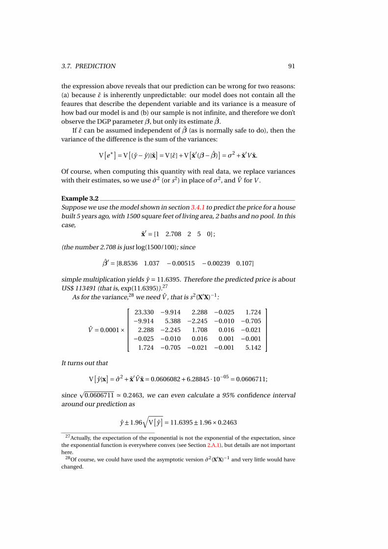
3.7. PREDICTION 91
the expression above reveals that our prediction can be wrong for two reasons:(a) because ε is inherently unpredictable: our model does not contain all thefeaures that describe the dependent variable and its variance is a measure ofhow bad our model is and (b) our sample is not infinite, and therefore we don’tobserve the DGP parameter β, but only its estimate β.
If ε can be assumed independent of β (as is normally safe to do), then thevariance of the difference is the sum of the variances:
V[e∗
]= V[(y − y)|x]= V[ε]+V
[x′(β− β)
]=σ2 + x′V x.
Of course, when computing this quantity with real data, we replace varianceswith their estimates, so we use σ2 (or s2) in place of σ2, and V for V .
Example 3.2Suppose we use the model shown in section 3.4.1 to predict the price for a housebuilt 5 years ago, with 1500 square feet of living area, 2 baths and no pool. In thiscase,
x′ = [1 2.708 2 5 0] ;
(the number 2.708 is just log(1500/100); since
β′ = [8.8536 1.037 −0.00515 −0.00239 0.107]
simple multiplication yields y = 11.6395. Therefore the predicted price is aboutUS$ 113491 (that is, exp(11.6395)).27
As for the variance,28 we need V , that is s2(X′X)−1:
V = 0.0001×
23.330 −9.914 2.288 −0.025 1.724−9.914 5.388 −2.245 −0.010 −0.705
2.288 −2.245 1.708 0.016 −0.021−0.025 −0.010 0.016 0.001 −0.001
1.724 −0.705 −0.021 −0.001 5.142
It turns out that
V[
y |x]= σ2 + x′V x = 0.0606082+6.28845 ·10−05 = 0.0606711;
sincep
0.0606711 ' 0.2463, we can even calculate a 95% confidence intervalaround our prediction as
y ±1.96√
V[
y]= 11.6395±1.96×0.2463
27Actually, the expectation of the exponential is not the exponential of the expectation, sincethe exponential function is everywhere convex (see Section 2.A.1), but details are not importanthere.
28Of course, we could have used the asymptotic version σ2(X′X)−1 and very little would havechanged.
92 CHAPTER 3. USING OLS AS AN INFERENTIAL TOOL
so we could expect that, with a probability of 0.95, the log price of our hypothet-ical house would be between 11.157 and 12.122, and therefore the price itselfbetween $ 70000 and $ 180000 (roughly). You may feel unimpressed by such awide range, and I wouldn’t disagree. But on the other hand, consider that thisis a very basic model, which only takes into account very few features of theproperty, so it would be foolish to expect it to be razor-sharp when it comes toprediction.
One last thing: you may have noticed, in the example above, that the vari-ance of the predictor depends almost entirely on the “model uncertainty” com-ponent σ2 and very little on the “parameter uncertainty” component x′V x. Thisis not surprising, in the light of the fact that, as n → ∞, the latter componentshould vanish, since β is consistent. Therefore, in many settings (notably, intime-series models, that we’ll deal with in Chapter 5), the uncertainty on theprediction is tacitly assumed to come only from σ2.
3.8 The so-called “omitted-variable bias”
In many econometrics textbooks, you can find an argument that goes more orless like this: assume that the true model is
yi = xiβ1 + ziβ2 +εi ; (3.34)
if you try to estimate β1 via a regression of yi on xi alone, you’re going to end upwith a bad estimate. The proof is rather easy:29
β1 =∑n
i=1 xi yi∑ni=1 x2
i
=∑n
i=1 xi(xiβ1 + ziβ2 +εi
)∑ni=1 x2
i
= (3.35)
= β1 +β2
∑ni=1 xi zi∑n
i=1 x2i
+∑n
i=1 xiεi∑ni=1 x2
i
If you take probability limits, you’ll find that, even if E[εi |xi ] = 0,
β1p−→β1 +β2
E[xi zi ]
E[x2
i
]and the estimator would be inconsistent unless β2 = 0 and/or E[xi zi ] = 0. Thesolemn maxim the student receives at this point is “if you omit a relevant regres-sor (zi in our case, that is relevant ifβ2 6= 0) then your estimates will be incorrect,unless the omitted variable miraculously happens to be uncorrelated with xi ”.The phenomenon is usually called omitted variable bias.
29I could extend this example to matrices, but it would be totally unnecessary to grasp my point.
3.8. THE SO-CALLED “OMITTED-VARIABLE BIAS” 93
I’ve always considered this remark quite useless, if not outright misleading,and seeing econometricians, who are far better than myself, repeating it overand over to generations of students is a constant source of wonder to me. I’ll tryto illustrate why, and convince you of my point.
The parameter β1 in (3.34) is defined as the partial effect of xi on the condi-tional mean of yi on both xi and zi ; that is, the effect of x on y given z. It wouldbe silly to think that this quantity could be estimated consistently without us-ing any information on zi .30 The statistic β1, as defined in (3.35) (which doesignore zi ), is nevertheless a consistent estimator of a different quantity, namelythe partial effect of xi on the conditional mean of yi on xi alone, that is
E[
yi |xi]=β1xi +β2E[zi |xi ] .
The objection that some put forward, at this point, is: “OK; but assume thatequation (3.34) is my object of interest, and zi is unobservable, or unavailable.Surely, you must be aware that the estimate you get by using xi only is bogus.”Granted. But then, I may reply, do you ever get a real-life case when you observeall the variables you would like to have in your conditioning set? I don’t thinkso; take for example the model presented in section 3.4: in order to set up a trulycomplete model, you would have to have data on the state of the building, onthe quality of life in the neighbourhood, on the pleasantness of the view, andso on. You should always keep in mind that the parameters of your model onlymake sense in the context of the observable explanatory variable that you usefor conditioning.31
This doesn’t mean that you should not worry about omitted variable bias atall. The message to remember is: the quantity we would like to measure (ideally)is “the effect of x on y all else being equal”; but what we measure by OLS is theeffect of x on y conditional on z. Clearly, in order to interpret our estimate theway we would like to, z should be as close to “all else” as possible, and if you omitrelevant factors from your analysis (by choice, or impossibility) you have to beextra careful in interpreting your results.
Example 3.3I downloaded some data from the World Development Indicators32 website. Thevariables I’m using for this example are
30I should add that if we had an observable variable wi , which we knew for certain to be uncor-related with zi , you could estimate β1 consistently via a technique called instrumental variableestimation, which is the object of Chapter 6.
31In fact, there is an interesting link the bias you get from variable omission and the one you getfrom endogeneity (see section 3.5). Maybe I’ll write it down at some point.
32The World Development Indicator (or WDI for short) is a wonderful database, maintainedby the World Bank, that collects a wide variety of variables for over 200 countries over a largetime span. It is one of the most widely used resources in development economics and is publiclyavailable at http://wdi.worldbank.org or through DBnomics https://db.nomics.world/.
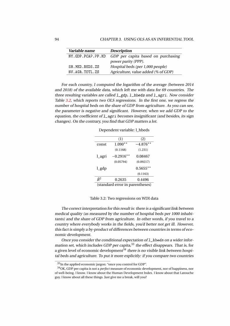
94 CHAPTER 3. USING OLS AS AN INFERENTIAL TOOL
Variable name DescriptionNY.GDP.PCAP.PP.KD GDP per capita based on purchasing
power parity (PPP).SH.MED.BEDS.ZS Hospital beds (per 1,000 people)NV.AGR.TOTL.ZS Agriculture, value added (% of GDP)
For each country, I computed the logarithm of the average (between 2014and 2018) of the available data, which left me with data for 69 countries. Thethree resulting variables are called l_gdp, l_hbeds and l_agri. Now considerTable 3.2, which reports two OLS regressions. In the first one, we regress thenumber of hospital beds on the share of GDP from agriculture. As you can see,the parameter is negative and significant. However, when we add GDP to theequation, the coefficient of l_agri becomes insignificant (and besides, its signchanges). On the contrary, you find that GDP matters a lot.
Dependent variable: l_hbeds
(1) (2)const 1.090∗∗ −4.876∗∗
(0.1168) (1.231)
l_agri −0.2916∗∗ 0.08467(0.05794) (0.09217)
l_gdp 0.5655∗∗
(0.1163)
R2 0.2635 0.4496(standard error in parentheses)
Table 3.2: Two regressions on WDI data
The correct interpretation for this result is: there is a significant link betweenmedical quality (as measured by the number of hospital beds per 1000 inhabi-tants) and the share of GDP from agriculture. In other words, if you travel to acountry where everybody works in the fields, you’d better not get ill. However,this fact is simply a by-product of differences between countries in terms of eco-nomic development.
Once you consider the conditional expectation of l_hbeds on a wider infor-mation set, which includes GDP per capita,33 the effect disappears. That is, fora given level of economic development34 there is no visible link between hospi-tal beds and agriculture. To put it more explicitly: if you compare two countries
33In the applied economic jargon: “once you control for GDP”.34OK, GDP per capita is not a perfect measure of economic development, nor of happiness, nor
of well-being. I know. I know about the Human Development Index. I know about that Latoucheguy. I know about all these things. Just give me a break, will you?
3.A. ASSORTED RESULTS 95
where the agricultural sectors have a different size (say, Singapore and Burundi),you’re likely to find differences in their health system quality. However, if youcompare two countries with the same per capita GDP (say, Croatia vs Greece, orVietnam vs Bolivia) you shouldn’t expect to find any association between agri-culture and hospital beds.
Does this mean that model (1) is “wrong”? No: it simply means that the twocoefficients in the two models measure two different things: a “gross” effect inequation (1) and a “net” effect in equation (2).35 Does this mean that model (2)is preferable? Yes: model (2) gives you a richer picture (see how much larger R2
is) because it’s based on a larger information set.
3.A Assorted results
3.A.1 Consistency of σ2
From (3.2), e = MXy = MXε. Therefore, the sum of squared residuals can be writ-ten as
e′e = ε′MXε= ε′ε−ε′X(X′X)−1X′ε;
now, given the definition of σ2,
σ2 = e′en
,
divide everything by n and take probability limits; the first bit is easy:
ε′εn
= 1
n
n∑i=1
ε2i
p−→ E[ε2
i
]=σ2.
On the other hand, equations (3.7) and (3.8) say that
ε′Xn
p−→ 0X′Xn
p−→Q
and therefore
σ2 = ε′MXε
n= ε
′εn
− ε′Xn
(X′Xn
)−1 X′εn
p−→ σ2 −0′Q−1 ·0 =σ2.
3.A.2 The Gauss-Markov theorem
The Gauss-Markov theorem states that, under homoskedasticity, OLS is the mostefficient estimator among all those that are (a) unbiased and (b) linear. Unbi-asedness means that E
[β
]=β; linearity means that β can be written as β = L′y.The OLS statistic enjoys both properties (L′ being equal to (X′X)−1X′ for OLS), but
35The discerning reader will doubtlessly spot the parallel with the discussion we had on theFrisch-Waugh theorem in section 1.5.
96 CHAPTER 3. USING OLS AS AN INFERENTIAL TOOL
other statistics may too. This property is often condensed in the phrase “OLS isBLUE”, where BLUE stands for “Best Linear Unbiased Estimator”.
The proof is simple if we concentrate on the case when X is a matrix of fixedconstants and does not contain random variables, because in this case we canshuffle X in and out of the expectation operator E[·] any way we want. Consider-ing the case when X contains random variables makes the proof more involved.
Here goes: take a linear estimator β defined as β = L′y. In order for it to beunbiased, the following must hold
E[β
]= E[L′ (Xβ+ε)]= L′Xβ+L′E[ε] =β;
it is safe to assume that E[ε] = 0, so the unbiasedness requirement amounts toL′X = I . Note that, in the standard case, there are infinitely many matrices thatsatisfy this requirement, since n > k and X is a “tall” matrix. In the OLS case,L′ = (X′X)−1X′, and the requirement is met. Therefore, under unbiasedness, βcan be written as β =β+L′ε.
Now consider the variance of β:
V[β
]= E[(β−β)(β−β)′
]= E[L′εε′L
]= L′E[εε′
]L = L V[ε] L′;
under homoskedasticity, V[ε] =σ2I , so
V[β
]=σ2L′L; (3.36)
again, OLS is just a special case, so the variance of β is easy to compute as V[β
]=σ2
[(X′X)−1X′][
X(X′X)−1]=σ2(X′X)−1.
The gist of the theorem lies in proving that the difference
V[β
]−V[β
]=σ2L′L−σ2(X′X)−1 =σ2 [L′L− (X′X)−1]
is positive semidefinite any time L 6= (X′X)−1X′, and therefore OLS is more effi-cient than β. This is relatively easy: define D ≡ L′− (X′X)−1X′, which has to benonzero unless β = β. Therefore, D′D must be positive semidefinite (see section1.A.7).
D′D = [L′− (X′X)−1X′][
L−X(X′X)−1]= L′L− (X′X)−1X′L−L′X(X′X)−1 + (X′X)−1;
under unbiasedness, L′X = X′L = I , so the expression above becomes
D′D = L′L− (X′X)−1 (3.37)
and the claim is proven.Having said this, let me add that the relevance of the Gauss-Markov theorem
in modern econometrics is quite limited: the assumption that X is a fixed matrixmakes sense in the context of a randomised experiment, but the data we havein economics are rarely compatible with this idea; the same goes, perhaps even
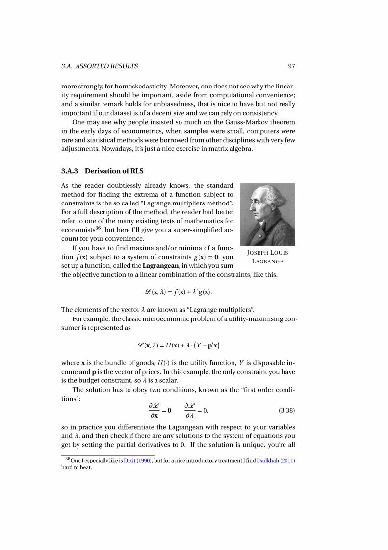
3.A. ASSORTED RESULTS 97
more strongly, for homoskedasticity. Moreover, one does not see why the linear-ity requirement should be important, aside from computational convenience;and a similar remark holds for unbiasedness, that is nice to have but not reallyimportant if our dataset is of a decent size and we can rely on consistency.
One may see why people insisted so much on the Gauss-Markov theoremin the early days of econometrics, when samples were small, computers wererare and statistical methods were borrowed from other disciplines with very fewadjustments. Nowadays, it’s just a nice exercise in matrix algebra.
3.A.3 Derivation of RLS
JOSEPH LOUIS
LAGRANGE
As the reader doubtlessly already knows, the standardmethod for finding the extrema of a function subject toconstraints is the so called “Lagrange multipliers method”.For a full description of the method, the reader had betterrefer to one of the many existing texts of mathematics foreconomists36, but here I’ll give you a super-simplified ac-count for your convenience.
If you have to find maxima and/or minima of a func-tion f (x) subject to a system of constraints g (x) = 0, youset up a function, called the Lagrangean, in which you sumthe objective function to a linear combination of the constraints, like this:
L (x,λ) = f (x)+λ′g (x).
The elements of the vector λ are known as “Lagrange multipliers”.For example, the classic microeconomic problem of a utility-maximising con-
sumer is represented as
L (x,λ) =U (x)+λ · (Y −p′x)
where x is the bundle of goods, U (·) is the utility function, Y is disposable in-come and p is the vector of prices. In this example, the only constraint you haveis the budget constraint, so λ is a scalar.
The solution has to obey two conditions, known as the “first order condi-tions”:
∂L
∂x= 0
∂L
∂λ= 0, (3.38)
so in practice you differentiate the Lagrangean with respect to your variablesand λ, and then check if there are any solutions to the system of equations youget by setting the partial derivatives to 0. If the solution is unique, you’re all
36One I especially like is Dixit (1990), but for a nice introductory treatment I find Dadkhah (2011)hard to beat.
98 CHAPTER 3. USING OLS AS AN INFERENTIAL TOOL
set. In the utility function example, applying equations (3.38) gives the standardmicroeconomic textbook solution to the problem:
∂U (x)
∂x=λp Y = p′x.
in words: at the maximum, (a) marginal utilities are proportional to prices (or∂U∂xi
/∂U∂x j
= pi
p jif you prefer) and (b) you should spend all your income.
In the case of RLS, the Lagrangean is37
L (β,λ) = 1
2e′e+λ′(Rβ−d).
where of course e = y − Xβ. The derivative of L with respect to λ is just theconstraint; as for the other one, since the derivative of e with respect to β is −X,we can use the chain rule like in section 1.A.5, arranging all the products in anappropriate way so as to obtain column vectors, which gives
∂L
∂β=−X′e+R ′λ
so the first order condition with respect to β can be written as
X′e = R ′λ, (3.39)
where e is the vector that satisfies equation (3.39), defined as y−Xβ. By premul-tiplying (3.39) by (X′X)−1 we get
(X′X)−1X′(y−Xβ) = β− β = (X′X)−1R ′λ,
which of course implies
β = β− (X′X)−1R ′λ (3.40)
So the constrained solution β can be expressed as the OLS vector β, plus a “cor-rection factor”, proportional to λ. If we premultiply (3.40) by R we get
λ= [R(X′X)−1R ′]−1
(Rβ−d) (3.41)
because Rβ = d by construction. Interestingly,λ itself is proportional to (Rβ−d),that is precisely the quantity we use for the construction of the W statistic in(3.18). Finally, equation (3.25) is obtained by combining (3.40) and (3.41):
β = β− (X′X)−1R ′ [R(X′X)−1R ′]−1(Rβ−d).
37Note that I divided the objective function by 2. Clearly, the solution is the same, but the alge-bra is somewhat simplified.
3.A. ASSORTED RESULTS 99
3.A.4 Asymptotic properties of the RLS estimator
Begin by (3.25)
β = β− (X′X)−1R ′ [R(X′X)−1R ′]−1(Rβ−d);
from this equation, it is quite easy to see that β is an affine function of β; thiswill be quite useful. Now define H as
H = plim((X′X)−1R ′ [R(X′X)−1R ′]−1
)=Q−1R ′ [RQ−1R ′]−1
(3.42)
normally, this is a (k ×p) matrix with rank p; also note that HR is idempotent.If β is consistent, then
βp−→β−H · (Rβ−d)
so if Rβ = d, consistency is guaranteed; otherwise, it isn’t.As for efficiency, let me briefly remind you what we mean by “efficiency”:38
an estimator a is more efficient than a competing estimator b if the differenceV (b)−V (a) is positive. If the two estimators are vectors, then the criterion gener-alises to the requirement that V (b)−V (a) is a positive semi-definite matrix (psdfor short — see section 1.A.7, especially figure 1.3).
There are a few matrix algebra results that we are going to need here:39
1. if A is pd, then A−1 is pd too;
2. if A is psd, then B ′AB is also psd for any matrix B .
Using these, we will prove that the asymptotic variance of β is smaller (in a ma-trix sense) that that for β:
AV[β
]= (I −HR) ·AV[β
] · (I −R ′H ′)
if AV[β
]=σ2Q−1, then note that
HRQ−1 =Q−1R ′ [RQ−1R ′]−1RQ−1, (3.43)
which is evidently symmetric, so HRQ−1 = Q−1R ′H ′; furthermore, by using thefact that HR is idempotent, you get
HRQ−1 = HRHRQ−1 = HRQ−1R ′H ′.
As a consequence, the asymptotic variance of β van be written as
AV[β
] = σ2 Q−1 −HRQ−1 −Q−1R ′H ′+HRQ−1R ′H ′=
= σ2 [Q−1 −HRQ−1]=
= AV[β
]−σ2HRQ−1
38A slightly fuller discussion is at the end of section 2.3.2.39They’re both easy to prove; try!
100 CHAPTER 3. USING OLS AS AN INFERENTIAL TOOL
the last thing we need do prove is that HRQ−1 is also positive semi-definite: forthis, we’ll use the right-hand side of (3.43).
Since Q is pd, then Q−1 is pd as well (property 1); therefore, RQ−1R ′ is alsopd (property 2), and so is
[RQ−1R ′]−1
(property 1). Finally, by using property
1 again, we find that Q−1R ′ [RQ−1R ′]−1RQ−1 is positive semi-definite and the
result follows.

Chapter 4
Diagnostic testing incross-sections
In order to justify the usage of OLS as an estimator, we made some assumptionsin section 3.2. Roughly:
1. the data we observe are realisations of random variables such that it makessense to assume that we are observing the same DGP in all the n casesin our dataset; or, more succinctly, there are no structural breaks in ourdataset.
2. We can trust asymptotic results as a reliable guide to the distribution ofour estimators, as the n observations we have are sufficiently homoge-neous and sufficiently independent, so that the LLN and the CLT can betaken as valid;
3. the conditional expectation E[
y |x]exists and is linear: E
[y |x]= x′β;
4. the conditional variance V[
y |x]exists and does not depend on x at all, so
it’s a positive constant: V[
y |x]=σ2.
Assumption number 2 may be inappropriate for two reasons: one is that oursample size is too small to justify asymptotic results as a reasonable approxima-tion to the actual properties of our statistics; the other one is that our observa-tion may not be identical, nor independent. The first case cannot really be testedformally; in most cases, the data we have are given and economists almost neverenjoy the privileges of experimenters, who can have as many data points as theywant (of course, given sufficient resources). Therefore, we just assume that ourdataset is good enough for our purposes, and hope for the best. Certainly, intel-lectual honesty dictates that we should be quite wary of drawing conclusions onthe basis of few data points, but there is not much more we can do. As for thesecond problem, we will defer the possible lack of independence to chapter 5,since the issue is most likely to arise with time-series data.
101
102 CHAPTER 4. DIAGNOSTIC TESTING IN CROSS-SECTIONS
In the next section, we will consider a way of testing assumptions 1 (to someextent) and 3. If they fail, consistency of β may be at risk. Conversely, assump-tion number 4 is crucial for our hypothesis testing apparatus, and will needsome extra tools; this will be the object of section 4.2.
4.1 Diagnostics for the conditional mean
Our main tool in proving that βp−→ β was that E
[y |x] = x′β (see section 3.2.1).
But this statement may be false. We will not explore the problem in its full gen-erality: we’ll just focus on two possible issues that often arise in practice.
1. the regression function is nonlinear, but can be approximated via a lin-ear function (see the discussion in section 1.3.2). In the case of a scalarregressor,
E[
yi |xi]= m(xi ) 'β0 +β1xi +β2x2
i +·· ·βq xqi =
q∑j=0
β j x ji .
2. Our data comprises observation for which the DGP is partly different. Thatis, we have j = 1. . .m separate sub-populations, for which
E[
yi |xi]= x′iβ j
where j is the class that observation i belongs to. For example, we havedata on European and American firms, and the vectorβ is different on thetwo sides of the Atlantic (in this case, m = 2).
4.1.1 The RESET test
As I repeated several times over, the hypothesis of linearity simply means thatE
[yi |xi
]can be written as a linear combination of observable variables. The
short phrase we use is: the model has to be linear in the parameters (see Section1.3.4 for a fuller discussion).
For example, suppose xi is a scalar; it is perfectly possible to accommodatesomething like
E[
yi |xi]=β1xi +β2x2
i ;
(to ease exposition, I am assuming here that the conditional mean has no con-stant term). Suppose that the expression above holds, but in the model we esti-mate the quadratic term x2
i is dropped. That is, we estimate a model like
yi = γxi +ui ;
by OLS, so that we would obtain a statistic γ defined as
γ= (x′x)−1x′y =∑n
i=1 xi yi∑ni=1 x2
i
.
4.1. DIAGNOSTICS FOR THE CONDITIONAL MEAN 103
Clearly, there is no value of γ that can make ui the difference between yi andE
[yi |xi
], so we can’t expect γ to have all the nice asymptotic properties that OLS
has. In fact, it can be proven that (in standard cases) the statistic γ does have alimit in probability, but the number it tends to is neitherβ1 nor a simple functionof it, so technically there is no way we can use γ to estimate β1 consistently.
The limit in probability of γ is technicallyknown as a pseudo-true value, which is far toocomplex a concept for me to attempt an expo-sition here. The inquisitive reader may want
to have a look at Cameron and Trivedi (2005),section 4.7 or (more technical) Gourieroux andMonfort (1995). The ultimate bible on this isWhite (1994).
In the present case, the remedy is elementary: add x2i to the list of your re-
gressors and, voilà, you get perfectly good CAN estimates of β1 and β2.1 How-ever, in a real-life case, where you have a vector of explanatory variables xi ,things are not so simple. In order to have quadratic effects, you should includeall possible cross-products between regressors. For example, a model like
yi =β0 +β1xi +β2zi +εi
would become
yi =β0 +β1xi +β2zi︸ ︷︷ ︸linear part
+β3x2i +β4xi · zi +β5z2
i︸ ︷︷ ︸quadratic part
+εi
and it’s very easy to show that the number of quadratic terms becomes rapidlyunmanageable for a realistic model: if the original model has k regressors thequadratic one can have up to k(k+1)
2 additional terms.2. I don’t think I have towarn the reader on how much of a headache it would be to incorporate cubic orquartic terms.
The RESET test (stands for REgression Specification Error Test) is a wayto check whether a given specification is likely to be rich enough to need noadditional nonlinear effects. The intuition is simple and powerful: instead ofaugmenting our model with all the possible order 2 terms (squares and cross-products), we just use the square of the fitted values, that is instead of x2
i , xi · zi
and z2i in the example above, we would use
y2i = (
β1xi + β2zi)2
.
Clearly, a similar strategy could be extended to cubic terms; in the exampleabove, we would replace the linear combination of x3
i , x2i · zi , xi · z2
i and z3i with
the simple scalar term y3i . Then, we just check if the added terms are significant;
since this is a test for addition of variables to a pre-existing model, the most con-venient way to perform the test is by using the LM statistic (see section 3.6.1).
1Of course, you’d have to be careful in computing your marginal effects, but if you have readsection 1.3.4, you know that, don’t you?
2The reader is invited to work out what happens for various values of k.
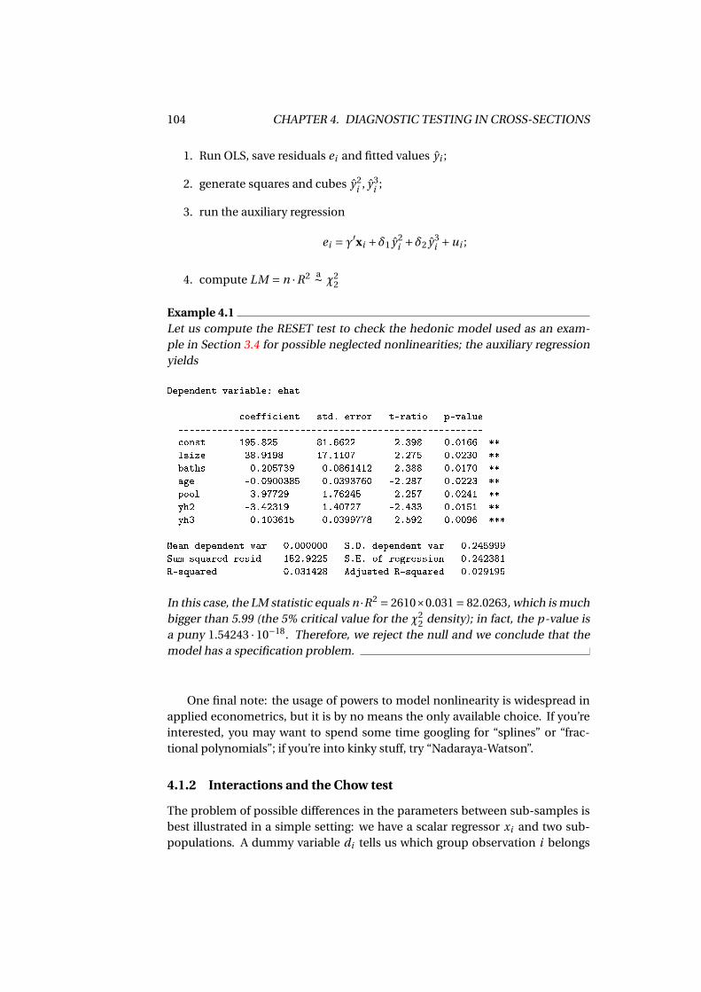
104 CHAPTER 4. DIAGNOSTIC TESTING IN CROSS-SECTIONS
1. Run OLS, save residuals ei and fitted values yi ;
2. generate squares and cubes y2i , y3
i ;
3. run the auxiliary regression
ei = γ′xi +δ1 y2i +δ2 y3
i +ui ;
4. compute LM = n ·R2 a∼ χ22
Example 4.1Let us compute the RESET test to check the hedonic model used as an exam-ple in Section 3.4 for possible neglected nonlinearities; the auxiliary regressionyields
Dependent variable: ehat
coefficient std. error t-ratio p-value
-------------------------------------------------------
const 195.825 81.6622 2.398 0.0166 **
lsize 38.9198 17.1107 2.275 0.0230 **
baths -0.205739 0.0861412 -2.388 0.0170 **
age -0.0900385 0.0393760 -2.287 0.0223 **
pool 3.97729 1.76245 2.257 0.0241 **
yh2 -3.42319 1.40727 -2.433 0.0151 **
yh3 0.103615 0.0399778 2.592 0.0096 ***
Mean dependent var 0.000000 S.D. dependent var 0.245999
Sum squared resid 152.9225 S.E. of regression 0.242381
R-squared 0.031428 Adjusted R-squared 0.029195
In this case, the LM statistic equals n ·R2 = 2610×0.031 = 82.0263, which is muchbigger than 5.99 (the 5% critical value for the χ2
2 density); in fact, the p-value isa puny 1.54243 · 10−18. Therefore, we reject the null and we conclude that themodel has a specification problem.
One final note: the usage of powers to model nonlinearity is widespread inapplied econometrics, but it is by no means the only available choice. If you’reinterested, you may want to spend some time googling for “splines” or “frac-tional polynomials”; if you’re into kinky stuff, try “Nadaraya-Watson”.
4.1.2 Interactions and the Chow test
The problem of possible differences in the parameters between sub-samples isbest illustrated in a simple setting: we have a scalar regressor xi and two sub-populations. A dummy variable di tells us which group observation i belongs
4.1. DIAGNOSTICS FOR THE CONDITIONAL MEAN 105
to. Suppose that the DGP could be described as follows:
Subsample 1 yi =β0 +β1xi +εi
Subsample 2 yi =β0 +β2xi +εi
with di = 0 in subsample 1 and di = 1 in subsample 2. Note that the model couldbe rewritten as
yi =β0 +[β1 + (β2 −β1)di
]xi +εi =β0 +β1xi +γdi · xi +εi (4.1)
where γ=β2 −β1. If the effect of xi on yi is in fact homogeneous across the twocategories, then γ= 0; therefore, testing for the equality of β1 and β2 is easy: allyou need to do is check whether the regressor di · xi is significant. Explanatoryvariables of this kind, that you obtain by multiplying a regressor by a dummyvariable, are often called interactions in the applied economics jargon. If theinteraction term turns out to be significant, then the effect of x on y is differentacross the two subcategories, since the interaction term in your model measureshow different the effect is across the two subgroups.
Clearly, you can interact as many regressors as you want: in the exampleabove, you could also imagine that the intercept could be different across thetwo subpopulations as well, so the model would become something like
yi =β0 +β1xi +γ0di +γ1di · xi +εi ,
because interacting the constant by di just gives you di .It should be noted that interactions can be viewed as including a peculiar
form of nonlinearity, so that you need to remeber this when computing marginaleffects. The marginal effect for xi in equation (4.1), for example, would be
∂E[
yi |xi]
∂xi=β+γdi ,
that is, β if di = 0 and β+γ if di = 1.Generalising this idea is not difficult: if you have m categories and you split
the vector xi into xi (constant effect across sub-populations) and xi (possiblydifferent effect across sub-populations) you can write the model as
yi = x′iγ+m∑
j=1(d j i xi )′γ j +εi
where d j i = 1 if observation i belongs to sub-population j , and 0 otherwise. Anequivalent (and much more often used) formulation is
yi = x′iβ+ ∑j 6=q
(d j i xi )′γ j +εi ; (4.2)
the proof of the equation above, if you’re interested, is in section 4.A.1. In prac-tice, you choose one subpopulation as the “reference” category (q in the equa-tion above), and the γ j coefficients measure the difference between the j -thcategory and the benchmark.
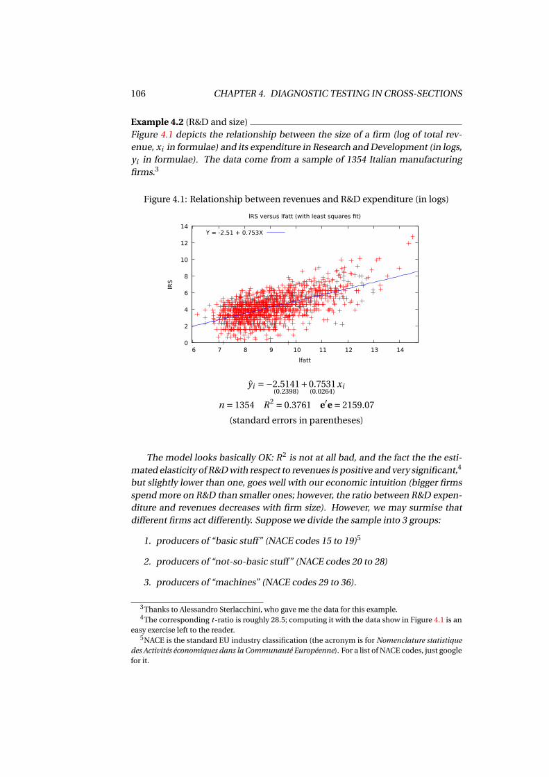
106 CHAPTER 4. DIAGNOSTIC TESTING IN CROSS-SECTIONS
Example 4.2 (R&D and size)Figure 4.1 depicts the relationship between the size of a firm (log of total rev-enue, xi in formulae) and its expenditure in Research and Development (in logs,yi in formulae). The data come from a sample of 1354 Italian manufacturingfirms.3
Figure 4.1: Relationship between revenues and R&D expenditure (in logs)
0
2
4
6
8
10
12
14
6 7 8 9 10 11 12 13 14
lRS
lfatt
lRS versus lfatt (with least squares fit)
Y = -2.51 + 0.753X
yi =−2.5141(0.2398)
+0.7531(0.0264)
xi
n = 1354 R2 = 0.3761 e′e = 2159.07
(standard errors in parentheses)
The model looks basically OK: R2 is not at all bad, and the fact the the esti-mated elasticity of R&D with respect to revenues is positive and very significant,4
but slightly lower than one, goes well with our economic intuition (bigger firmsspend more on R&D than smaller ones; however, the ratio between R&D expen-diture and revenues decreases with firm size). However, we may surmise thatdifferent firms act differently. Suppose we divide the sample into 3 groups:
1. producers of “basic stuff” (NACE codes 15 to 19)5
2. producers of “not-so-basic stuff” (NACE codes 20 to 28)
3. producers of “machines” (NACE codes 29 to 36).
3Thanks to Alessandro Sterlacchini, who gave me the data for this example.4The corresponding t-ratio is roughly 28.5; computing it with the data show in Figure 4.1 is an
easy exercise left to the reader.5NACE is the standard EU industry classification (the acronym is for Nomenclature statistique
des Activités économiques dans la Communauté Européenne). For a list of NACE codes, just googlefor it.
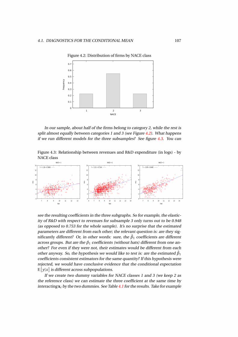
4.1. DIAGNOSTICS FOR THE CONDITIONAL MEAN 107
Figure 4.2: Distribution of firms by NACE class
0
0.1
0.2
0.3
0.4
0.5
0.6
0.7
1 2 3
frequency
NACE
In our sample, about half of the firms belong to category 2, while the rest issplit almost equally between categories 1 and 3 (see Figure 4.2). What happensif we run different models for the three subsamples? See figure 4.3. You can
Figure 4.3: Relationship between revenues and R&D expenditure (in logs) - byNACE class
0
2
4
6
8
10
12
14
7 8 9 10 11 12 13
lRS
lfatt
NACE = 1
Y = -1.38 + 0.588X
0
2
4
6
8
10
12
14
6 7 8 9 10 11 12 13 14
lRS
lfatt
NACE = 2
Y = -2.22 + 0.724X
0
2
4
6
8
10
12
14
7 8 9 10 11 12 13 14
lRS
lfatt
NACE = 3
Y = -3.99 + 0.948X
see the resulting coefficients in the three subgraphs. So for example, the elastic-ity of R&D with respect to revenues for subsample 3 only turns out to be 0.948(as opposed to 0.753 for the whole sample). It’s no surprise that the estimatedparameters are different from each other; the relevant question is: are they sig-nificantly different? Or, in other words: sure, the β1 coefficients are differentacross groups. But are the β1 coefficients (without hats) different from one an-other? For even if they were not, their estimates would be different from eachother anyway. So, the hypothesis we would like to test is: are the estimated β1
coefficients consistent estimators for the same quantity? If this hypothesis wererejected, we would have conclusive evidence that the conditional expectationE
[y |x]
is different across subpopulations.
If we create two dummy variables for NACE classes 1 and 3 (we keep 2 asthe reference class) we can estimate the three coefficient at the same time byinteracting xi by the two dummies. See Table 4.1 for the results. Take for example
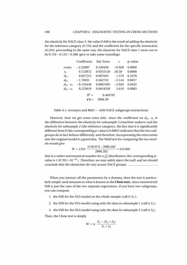
108 CHAPTER 4. DIAGNOSTIC TESTING IN CROSS-SECTIONS
the elasticity for NACE class 3: the value 0.948 is the result of adding the elasticityfor the reference category (0.724) and the coefficient for the specific interaction(0.224); proceeding in the same way, the elasticity for NACE class 1 turns out tobe 0.724−0.135 = 0.588 (give or take some rounding).
Coefficient Std. Error z p-value
const −2.22007 0.320450 −6.928 0.0000xi 0.723872 0.0353120 20.50 0.0000d1i 0.837215 0.607043 1.379 0.1678d3i −1.76931 0.562752 −3.144 0.0017d1i · xi −0.135458 0.0667693 −2.029 0.0425d3i · xi 0.223810 0.0618350 3.619 0.0003
R2 = 0.404707e′e = 2060.20
Table 4.1: revenues and R&D — with NACE subgroups interactions
However, here we get some extra info: since the coefficient on d3i · xi isthe difference between the elasticity for subsample 3 (machine makers) and theelasticity for subsample 2 (the reference category), the fact that it is significantlydifferent from 0 (the corresponding p-value is 0.0003) indicates that the two sub-groups do in fact behave differently, and therefore, incorporating the extra termsinto the original model is a good idea. The Wald test for comparing the two mod-els would give
W = 1354 · 2159.074−2060.202
2060.202= 224.602
that is a rather astronomical number for a χ24 distribution (the corresponding p-
value is 1.91703×10−47). Therefore, we may safely reject the null, and we shouldconclude that the elasticities do vary across NACE groups.
When you interact all the parameters by a dummy, then the test is particu-larly simple (and amounts to what is known as the Chow test), since unrestrictedSSR is just the sum of the two separate regressions: if you have two subgroups,you can compute
1. the SSR for the OLS model on the whole sample (call it ST );
2. the SSR for the OLS model using only the data in subsample 1 (call it S1);
3. the SSR for the OLS model using only the data in subsample 2 (call it S2).
Then, the Chow test is simply
W = n · ST − (S1 +S2)
S1 +S2
4.2. HETEROSKEDASTICITY AND ITS CONSEQUENCES 109
because the SSR for the model with all the interactions is equal to the sum ofthe SSRs for the separate submodels. In fact, this result holds for any number ofsubcategories; the proof is in subsection 4.A.2.
4.2 Heteroskedasticity and its consequences
As the reader might recall, the homoskedasticity assumption was a fundamen-tal ingredient in the derivation of the asymptotic covariance matrix of the OLSestimator (see 3.2). While the linearity assumption E
[y |x] = x′β makes consis-
tency almost automatic (E[ε ·x] = 0 implies βp−→ β if some kind of LLN can be
invoked), it’s impossible to derive the parallel result for asymptotic normality
pn
(β−β) p−→ N
[0,σ2Q−1]
without assuming homoskedasticity, that is E[ε2|x]=σ2.
Like all assumptions, homoskedasticity is easier to justify in certain circum-stances than others. If data come from controlled experiments, εi can often beinterpreted as the disturbance term that contaminated the i -th experiment; itis normally safe to think that εi should be independent from xi , the conditionsunder which the experiment was performed. Therefore, if εi ⊥⊥ xi , no momentsof εi can depend on xi , and homoskedasticity follows.
This is almost never the case in economics, where virtually all data comefrom non-experimental settings. This is particularly true for cross-sectional data,where we collect data about individuals who did not take part in an experimentat all. When we estimate a wage equation, our dependent variable yi (typically,the log wage for individual i ) will be matched against a vector of explanatoryvariables xi that contain a description of that individual (education, age, workexperience and so on), and εi is simply defined as the deviation of yi from itsconditional expectation, so in principle there is no reason to think that it shouldenjoy any special properties except E[εi |xi ] = 0, which holds by constructionunder the linearity hypothesis.
Therefore, assuming that εi has a finite second moment, in general all wecan say is that E
[ε2
i |xi]
is some function of xi :
E[ε2
i |xi]= h(xi ) =σ2
i , (4.3)
where the function h(·) is of unknown form (but certainly non-linear, since σ2i
can never be negative). Since the variances σ2i may be different across observa-
tions, we use the term heteroskedasticity.To simplify notation, in this section all expectation operators will be implic-
itly understood as conditional on X. In other words, we will treat X as if it were amatrix of constants. Therefore,
y = Xβ+ε V[ε] = E[εε′
]=Σ
110 CHAPTER 4. DIAGNOSTIC TESTING IN CROSS-SECTIONS
If our model is heteroskedastic, then Σ is a diagonal matrix, where elementsalong the main diagonal need not be equal to each other, and it would look likethis:6
σ21
σ22
. . .
σ2n
The variance of β can be simply computed as
V[β
]= V[β+ (X′X)−1X′ε
]= (X′X)−1 X′ΣX (X′X)−1 (4.4)
and clearly if Σ = σ2I we go back to σ2(X′X)−1. But under heteroskedasticitythe V = σ2(X′X)−1 matrix may be very far from the actual asymptotic covariancematrix of β (shown in equation (4.4)), even asymptotically; therefore, our teststatistics are very unlikely to be χ2-distributed under H0, which makes our p-values all wrong and inference impossible.
In order to see how the situation can be remedied, it’s instructive to considera case of limited practical relevance, but that provides a few insights that mayhelp later: the case when Σ is known.
4.2.1 If Σwere known
If the matrix Σwere observable, then theσ2i variances would be known (they are
just the diagonal elements of Σ), and getting rid of heteroskedasticity would beeasy: define
yi = yi
σixi = 1
σixi ui = εi
σi
and the model becomesyi = x′iβ+ui
but clearly V[ui ] = 1 by construction,7 so you can happily run OLS on the trans-formed variables, since yi and xi would both be observable. The resulting esti-mator
β =[
n∑i=1
xi x′i
]−1 n∑i=1
xi yi = (X′X)−1X′y
could also be written as
β =[
n∑i=1
1
σ2i
xi x′i
]−1 n∑i=1
1
σ2i
xi yi = (X′Σ−1X)−1X′Σ−1y (4.5)
6In fact, some of our considerations carry over to more general cases, in which Σ is a genericsymmetric, positive semi-definite matrix, but let’s not complicate matters.
7Readers would hopefully not feel offended if I reminded them that a straightforward applica-tion of equation (2.6) yields V[X /b] = V[X ]/b2.
4.2. HETEROSKEDASTICITY AND ITS CONSEQUENCES 111
and is called GLS. It can be proven that GLS is more efficient than OLS (the proofis in subsection 4.A.3), and that its covariance matrix equals
V[β
]= (X′Σ−1X)−1
Since GLS is just OLS on suitably transformed variables, all standard propertiesof OLS in the homoskedastic case remain valid, so for example you could testhypotheses by the usual techniques.8
Of course, in ordinary circumstances Σ is unknown, but we could use thisidea to explore alternative avenues:
1. In some cases, you may have reason to believe that σ2i should be roughly
proportional to some observable variable. For example, if yi is an averagefrom some sampled values and ni is the size of the i -th sample, it wouldbe rather natural to conjecture that σ2
i ' K n−1i , where K is some constant.
Therefore, by dividing all the observables byp
ni you get an equivalentrepresentation of the model, in which heteroskedasticity is less likely to bea problem, since in the transformed model all variances should be roughlyequal to K . The resulting estimator is sometimes called WLS (for WeightedLeast Squares), because you “weight” each observation by an observablequantity wi . In our example, wi =
p1/ni .
2. The idea above can be generalised: one could try to reformulate the modelin such a way that the heteroskedasticity problem might be attenuated.For example, it is often the case that, rather than a model like
Yi =α0 +α1Xi +ui ,
a formulation in natural logs, like
lnYi =β0 +β1 ln Xi +εi
not only leads to a more natural interpretation of the parameters (since β1
can be read as an elasticity), but also alleviates heteroskedasticity prob-lems.
3. Even more generally, it can be proven that, if we have Σp−→ Σ, we can use
it in the so-called “feasible” version of GLS, or FGLS for short:
β = (X′Σ−1X)−1X′Σ−1y
but this is normally accomplished by setting an explicit functional formfor the conditional variance (the function h(·) in 4.3). It can be done, but
8In fact, we wouldn’t even have to observe Σ, as long as we had a matrix which is proportionalto Σ by a (possibly unknown) scalar factor. If we had Ω = c ·Σ, where c is an unknown positivescalar, we could useΩ instead of Σ in equation (4.5), since the scalar c would cancel out.
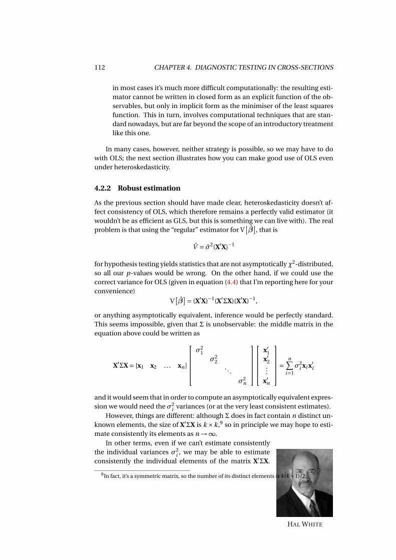
112 CHAPTER 4. DIAGNOSTIC TESTING IN CROSS-SECTIONS
in most cases it’s much more difficult computationally: the resulting esti-mator cannot be written in closed form as an explicit function of the ob-servables, but only in implicit form as the minimiser of the least squaresfunction. This in turn, involves computational techniques that are stan-dard nowadays, but are far beyond the scope of an introductory treatmentlike this one.
In many cases, however, neither strategy is possible, so we may have to dowith OLS; the next section illustrates how you can make good use of OLS evenunder heteroskedasticity.
4.2.2 Robust estimation
As the previous section should have made clear, heteroskedasticity doesn’t af-fect consistency of OLS, which therefore remains a perfectly valid estimator (itwouldn’t be as efficient as GLS, but this is something we can live with). The realproblem is that using the “regular” estimator for V
[β
], that is
V = σ2(X′X)−1
for hypothesis testing yields statistics that are not asymptotically χ2-distributed,so all our p-values would be wrong. On the other hand, if we could use thecorrect variance for OLS (given in equation (4.4) that I’m reporting here for yourconvenience)
V[β
]= (X′X)−1(X′ΣX)(X′X)−1,
or anything asymptotically equivalent, inference would be perfectly standard.This seems impossible, given that Σ is unobservable: the middle matrix in theequation above could be written as
X′ΣX = [x1 x2 . . . xn]
σ2
1σ2
2. . .
σ2n
x′1x′2...
x′n
=n∑
i=1σ2
i xi x′i
and it would seem that in order to compute an asymptotically equivalent expres-sion we would need the σ2
i variances (or at the very least consistent estimates).However, things are different: although Σ does in fact contain n distinct un-
known elements, the size of X′ΣX is k ×k,9 so in principle we may hope to esti-mate consistently its elements as n →∞.
HAL WHITE
In other terms, even if we can’t estimate consistentlythe individual variances σ2
i , we may be able to estimateconsistently the individual elements of the matrix X′ΣX.
9In fact, it’s a symmetric matrix, so the number of its distinct elements is k(k +1)/2.
4.2. HETEROSKEDASTICITY AND ITS CONSEQUENCES 113
This is the basic idea that was put forward in White (1980):under heteroskedasticity, OLS is still consistent, so
βp−→β =⇒ ei = yi −x′i β
p−→ εi = yi −x′iβ =⇒ e2i
p−→ ε2i :
the difference between the OLS residuals ei and the dis-turbances εi should be “small” in large samples. Sinceσ2
i = E(ε2i ), we’d expect that the average of e2
i −σ2i should
also be a small quantity. Therefore,
1
n
n∑i=1
(e2i −σ2
i )xi x′ip−→ [0],
where I’m using the [0] notation for “a matrix full of zeros”. Now rewrite (4.4) as
V[β
]= (X′X)−1
(n∑
i=1σ2
i xi x′i
)(X′X)−1
Therefore, asymptotically you can estimate V[β
]via
V = (X′X)−1
(n∑
i=1e2
i xi x′i
)(X′X)−1 (4.6)
In fact, many variants have been proposed since White’s 1980 paper, thatseem to have better performance in finite samples, and most packages use oneof the later solutions. The principle they are based, on however, is still the origi-nal one.10
An even more radical solution for dealing with heteroskedasticity has be-come quite popular over the recent past because of the enormous advancementof our computing capabilities: it’s called the bootstrap. In many respects, thebootstrap is a very ingenious solution for performing inference with estimatorswhose covariance matrix could be unreliable, for various reasons. In a book likethis, giving a full account of the bootstrap is far too ambitious a task, and I’ll justgive you a cursory description in section 4.A.4. Nevertheless, the reader oughtto be aware that “bootstrapped standard errors” are becoming more and morewidely used in the applied literature.
Example 4.3The hedonic model presented in section 3.4 was re-estimated with robust stan-dard errors, and the results are shown in Table 4.2.
As the reader can check, all the figures in Table 4.2 are exactly the same asthose in Table 3.1, except for those that depend on the covariance matrix of
10A clever variation on the same principle that goes under the name of cluster-robust varianceestimation has become inexplicably popular in recent years. I’m not going to describe it in thisbook, but you should be aware that in some circles you will be treated like the village idiot if youdon’t “cluster your standard errors”. For more details, read Cameron and Miller (2015).
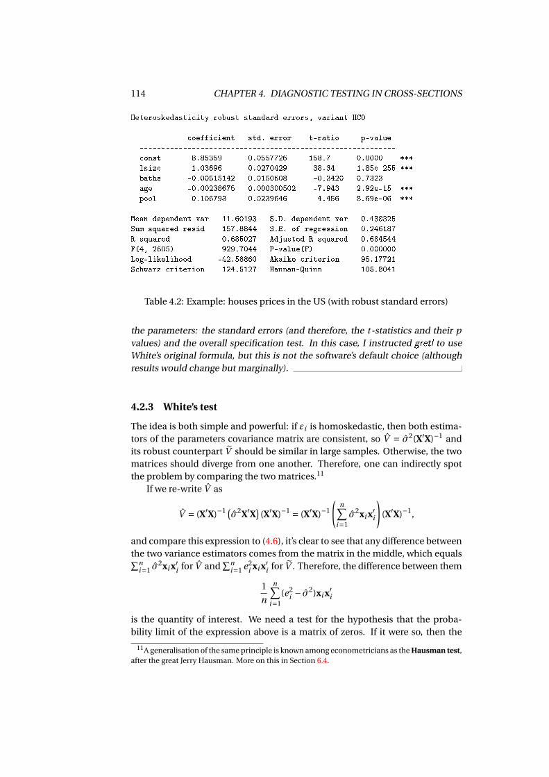
114 CHAPTER 4. DIAGNOSTIC TESTING IN CROSS-SECTIONS
Heteroskedasticity-robust standard errors, variant HC0
coefficient std. error t-ratio p-value
-----------------------------------------------------------
const 8.85359 0.0557726 158.7 0.0000 ***
lsize 1.03696 0.0270429 38.34 1.85e-255 ***
baths -0.00515142 0.0150608 -0.3420 0.7323
age -0.00238675 0.000300502 -7.943 2.92e-15 ***
pool 0.106793 0.0239646 4.456 8.69e-06 ***
Mean dependent var 11.60193 S.D. dependent var 0.438325
Sum squared resid 157.8844 S.E. of regression 0.246187
R-squared 0.685027 Adjusted R-squared 0.684544
F(4, 2605) 929.7044 P-value(F) 0.000000
Log-likelihood -42.58860 Akaike criterion 95.17721
Schwarz criterion 124.5127 Hannan-Quinn 105.8041
Table 4.2: Example: houses prices in the US (with robust standard errors)
the parameters: the standard errors (and therefore, the t-statistics and their pvalues) and the overall specification test. In this case, I instructed gretl to useWhite’s original formula, but this is not the software’s default choice (althoughresults would change but marginally).
4.2.3 White’s test
The idea is both simple and powerful: if εi is homoskedastic, then both estima-tors of the parameters covariance matrix are consistent, so V = σ2(X′X)−1 andits robust counterpart V should be similar in large samples. Otherwise, the twomatrices should diverge from one another. Therefore, one can indirectly spotthe problem by comparing the two matrices.11
If we re-write V as
V = (X′X)−1 (σ2X′X
)(X′X)−1 = (X′X)−1
(n∑
i=1σ2xi x′i
)(X′X)−1,
and compare this expression to (4.6), it’s clear to see that any difference betweenthe two variance estimators comes from the matrix in the middle, which equals∑n
i=1 σ2xi x′i for V and
∑ni=1 e2
i xi x′i for V . Therefore, the difference between them
1
n
n∑i=1
(e2i − σ2)xi x′i
is the quantity of interest. We need a test for the hypothesis that the proba-bility limit of the expression above is a matrix of zeros. If it were so, then the
11A generalisation of the same principle is known among econometricians as the Hausman test,after the great Jerry Hausman. More on this in Section 6.4.
4.2. HETEROSKEDASTICITY AND ITS CONSEQUENCES 115
two estimators would converge to the same limit, and therefore the two esti-mators would coincide asymptotically; this, of course, wouldn’t happen underheteroskedasticity. Therefore, the null hypothesis of White’s test is homoskedas-ticity.
It would seem that performing such a test is difficult; fortunately, an asymp-totically equivalent test is easy to compute by means of an auxiliary regression:
e2i = γ0 +z′iγ+ui ;
the vector zi contains the cross-products of xi , that is all combinations of thekind xl i · xmi (with l ,m = 1. . .k) that wouldn’t yield collinearity (an example isgiven below). Of course, if xi contains a constant term, then zi would contain allthe elements of xi , as the products 1 · xmi .
Like in all auxiliary regression, we don’t really care about its results; runningit is just a computationally convenient way to calculate the test statistic we need,namely
LM = n ·R2.
Under the null of homoskedasticity, this statistic will be asymptotically distributedas χ2
p , where p is the size of the vector zi .For example: suppose that xi contains:
1. the constant;
2. two continuous variables xi and wi ;
3. a dummy variable di
The cross products could be written as per the following “multiplication ta-ble”
1 xi wi di
1 1 xi wi di
xi xi x2i xi ·wi xi ·di
wi wi xi ·wi w2i wi ·di
di di xi ·di wi ·di di
where I indicated the elements to keep by shading the corresponding cell in grey.Of course the lower triangle is redundant, because it reproduces the upper one,but the element in the South-East corner must be dropped too: since di is adummy variable, it only contains zeros and ones, so its square d 2
i contains thesame entries as di itself; clearly, inserting both di and d 2
i into zi would make theauxiliary regression collinear.
Therefore, the vector zi would contain
z′i = [xi , wi , di , x2i , xi ·wi , xi ·di , w2
i , wi ·di ]
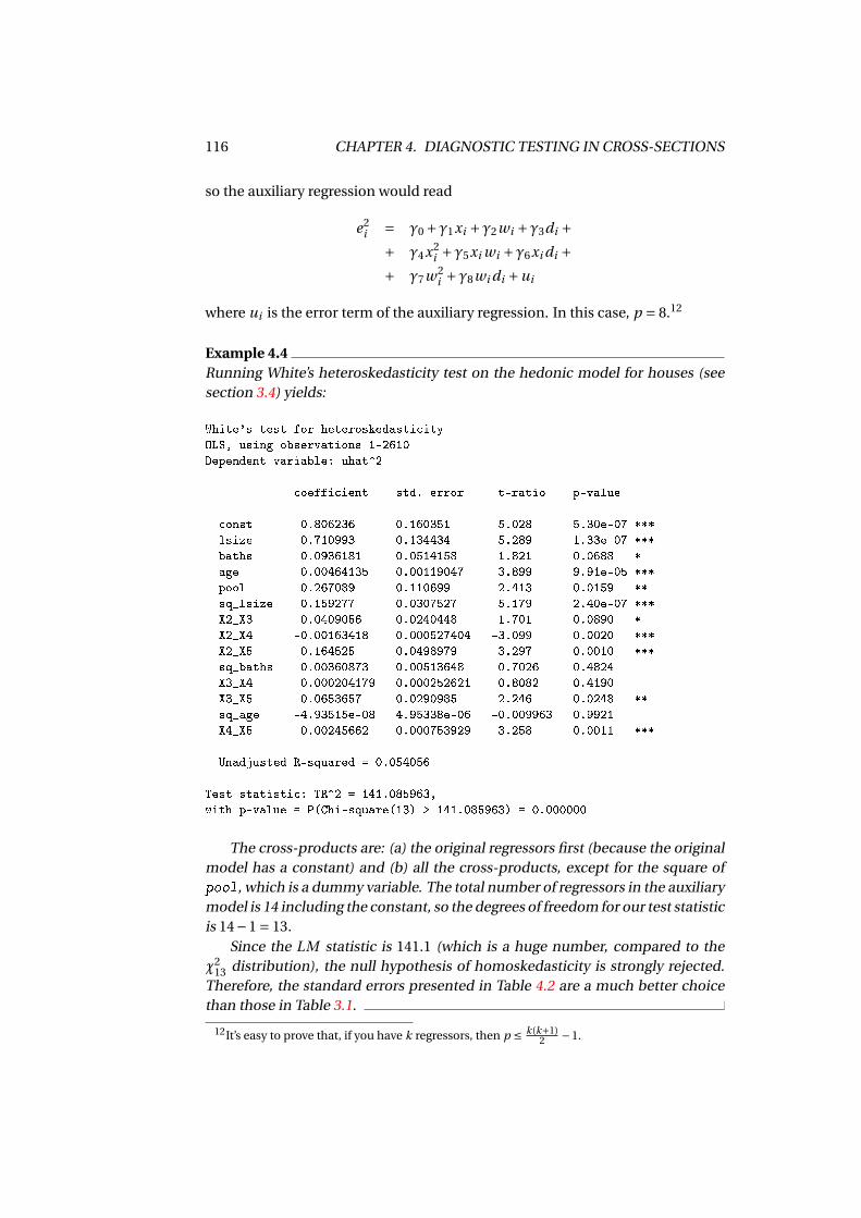
116 CHAPTER 4. DIAGNOSTIC TESTING IN CROSS-SECTIONS
so the auxiliary regression would read
e2i = γ0 +γ1xi +γ2wi +γ3di +
+ γ4x2i +γ5xi wi +γ6xi di +
+ γ7w2i +γ8wi di +ui
where ui is the error term of the auxiliary regression. In this case, p = 8.12
Example 4.4Running White’s heteroskedasticity test on the hedonic model for houses (seesection 3.4) yields:
White's test for heteroskedasticity
OLS, using observations 1-2610
Dependent variable: uhat^2
coefficient std. error t-ratio p-value
------------------------------------------------------------
const 0.806236 0.160351 5.028 5.30e-07 ***
lsize -0.710993 0.134434 -5.289 1.33e-07 ***
baths 0.0936181 0.0514158 1.821 0.0688 *
age 0.00464135 0.00119047 3.899 9.91e-05 ***
pool 0.267089 0.110699 2.413 0.0159 **
sq_lsize 0.159277 0.0307527 5.179 2.40e-07 ***
X2_X3 -0.0409056 0.0240448 -1.701 0.0890 *
X2_X4 -0.00163418 0.000527404 -3.099 0.0020 ***
X2_X5 -0.164525 0.0498979 -3.297 0.0010 ***
sq_baths 0.00360873 0.00513648 0.7026 0.4824
X3_X4 0.000204179 0.000252621 0.8082 0.4190
X3_X5 0.0653657 0.0290985 2.246 0.0248 **
sq_age -4.93515e-08 4.95338e-06 -0.009963 0.9921
X4_X5 0.00245662 0.000753929 3.258 0.0011 ***
Unadjusted R-squared = 0.054056
Test statistic: TR^2 = 141.085963,
with p-value = P(Chi-square(13) > 141.085963) = 0.000000
The cross-products are: (a) the original regressors first (because the originalmodel has a constant) and (b) all the cross-products, except for the square ofpool, which is a dummy variable. The total number of regressors in the auxiliarymodel is 14 including the constant, so the degrees of freedom for our test statisticis 14−1 = 13.
Since the LM statistic is 141.1 (which is a huge number, compared to theχ2
13 distribution), the null hypothesis of homoskedasticity is strongly rejected.Therefore, the standard errors presented in Table 4.2 are a much better choicethan those in Table 3.1.
12It’s easy to prove that, if you have k regressors, then p ≤ k(k+1)2 −1.
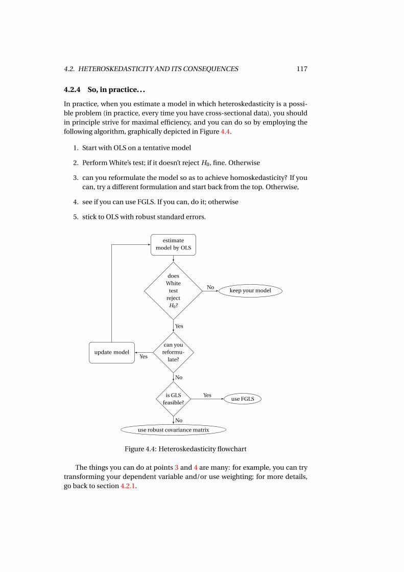
4.2. HETEROSKEDASTICITY AND ITS CONSEQUENCES 117
4.2.4 So, in practice. . .
In practice, when you estimate a model in which heteroskedasticity is a possi-ble problem (in practice, every time you have cross-sectional data), you shouldin principle strive for maximal efficiency, and you can do so by employing thefollowing algorithm, graphically depicted in Figure 4.4.
1. Start with OLS on a tentative model
2. Perform White’s test; if it doesn’t reject H0, fine. Otherwise
3. can you reformulate the model so as to achieve homoskedasticity? If youcan, try a different formulation and start back from the top. Otherwise,
4. see if you can use FGLS. If you can, do it; otherwise
5. stick to OLS with robust standard errors.
estimatemodel by OLS
doesWhite
testreject
H0?
keep your model
can youreformu-
late?update model
is GLSfeasible?
use FGLS
use robust covariance matrix
No
Yes
Yes
No
Yes
No
Figure 4.4: Heteroskedasticity flowchart
The things you can do at points 3 and 4 are many: for example, you can trytransforming your dependent variable and/or use weighting; for more details,go back to section 4.2.1.
118 CHAPTER 4. DIAGNOSTIC TESTING IN CROSS-SECTIONS
Note, however, that this algorithm often ends at point 5; this is so com-mon that many people, in the applied economics community, don’t even botherchecking for heteroskedasticity and start directly from there.13 This is especiallytrue in some cases, where you know from the outset what the situation is. Theso-called linear probability model (often abbreviated as LPM) is a notable ex-ample.
The LPM is what you get when your dependent variable is a dummy. So forexample you may want to set up a model where yi is the employment status of anindividual, so yi = 1 if the i -th person has a job and yi = 0 otherwise. Contraryto what happens in most cases, we know exactly what the distribution of thedependent variable is: it’s a Bernoulli random variable:
yi =
1 with probability πi
0 with probability 1−πi(4.7)
The linearity hypothesis implies that E[
yi |xi]=πi = x′iβ, since for a Bernoulli
rv the expected value is, by construction, the probability of success. This is quiteweird already, because π is a probability, and therefore has to be between 0 and1, whereas if it really was a linear function of the x variables, you could alwaysimagine to find an observation for which the predicted probability is outsidethe [0,1] interval. Many applied econometricians are OK with that: they con-cede that the linearity assumption is inappropriate after all, but assume that itshouldn’t be a problem in practice, and use it as a convenient approximation.14
But then, you also have that for a Bernoulli rv V[
yi]=πi · (1−πi ), and there-
fore
V[
yi |xi]=πi = x′iβ · (1−x′iβi )
so the conditional variance cannot be constant unless the conditional mean isconstant too. The vector of parameters β enjoys a special nature, being the vec-tor of parameters that determine both the conditional mean and the conditionalvariance. In theory, it is be possible to estimate β by an elaborate FGLS strategy,but in these cases practitioners always just use OLS with robust standard errors.
13In fact, some researchers show sometimes an inclination to disregard specification issues inhope that robust inference will magically take care of everything, which is of course not the case.For an insightful analysis, see King and Roberts (2015).
14Models that overcome this questionable approach have existed for a long time: you’ll find athorough description of logit and probit models in any decent econometrics textbook, but forsome bizarre reason they are going out of fashion.
4.A. ASSORTED RESULTS 119
4.A Assorted results
4.A.1 Proof of equation (4.2)
We would like to prove that the two models
yi = x′iγ+m∑
j=1(d j i xi )′γ j +εi
andyi = x′iβ+ ∑
j 6=q(d j i xi )′γ j +εi
are equivalent. In order to do so, we will prove that the space spanned by theregressors of the two equations is the same. Without loss of generality, supposethat the observations are sorted so that all the cases for which d1i = 1 are on top,and then come those for which d2i = 1, and so on, so that the bottom rows of thedataset are the observations for which dmi = 1.
The regressors matrix for the first equation can then be written as
Z =
X1 X1 0 . . . 0X2 0 X2 . . . 0...
......
. . ....
Xm 0 0 . . . Xm
Suppose, again without loss of generality, that the reference category is the firstone; now substitute the second block of columns by the sum of the blocks for 2to the last. Call the resulting matrix W, where
W =
X1 X1 0 . . . 0X2 X2 X2 . . . 0...
......
. . ....
Xm Xm 0 . . . Xm
=
X1 0 . . . 0X2 X2 . . . 0...
.... . .
...Xm 0 . . . Xm
where the second equality trivially come from X j = [X j X j ]. It is clear that
• W is the regressors matrix for the second equation, and
• you can compute W from Z, but also Z from W; therefore, W can be writtenas W = Z · A, where A is invertible.
Therefore, Sp(Z) = Sp(W) (see section 1.A.8), so PZ = PW and the fitted valuesand the residuals from the two regressions are the same (see section 1.A.8).
For example, take the model
Subsample 1 yi =β0 +β1xi +εi
Subsample 2 yi =β0 +β2xi +εi ,
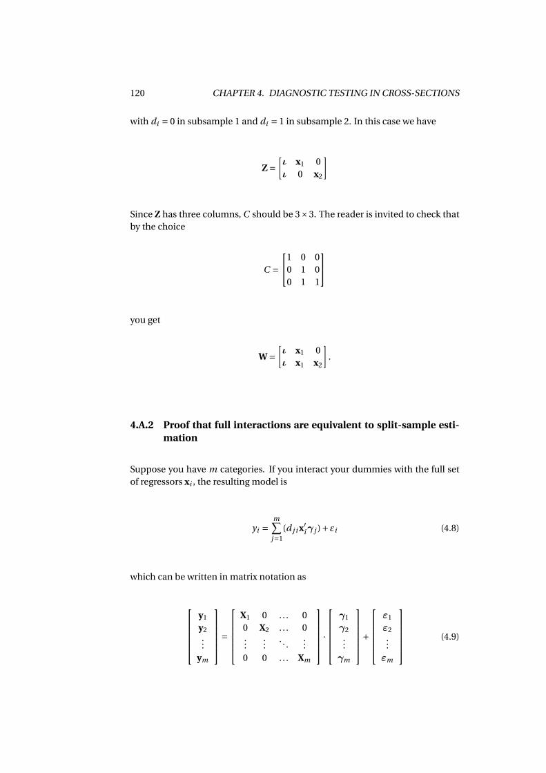
120 CHAPTER 4. DIAGNOSTIC TESTING IN CROSS-SECTIONS
with di = 0 in subsample 1 and di = 1 in subsample 2. In this case we have
Z =[ι x1 0ι 0 x2
]
Since Z has three columns, C should be 3×3. The reader is invited to check thatby the choice
C =1 0 0
0 1 00 1 1
you get
W =[ι x1 0ι x1 x2
].
4.A.2 Proof that full interactions are equivalent to split-sample esti-mation
Suppose you have m categories. If you interact your dummies with the full setof regressors xi , the resulting model is
yi =m∑
j=1(d j i x′iγ j )+εi (4.8)
which can be written in matrix notation as
y1
y2...
ym
=
X1 0 . . . 00 X2 . . . 0...
.... . .
...0 0 . . . Xm
·
γ1
γ2...γm
+
ε1
ε2...εm
(4.9)
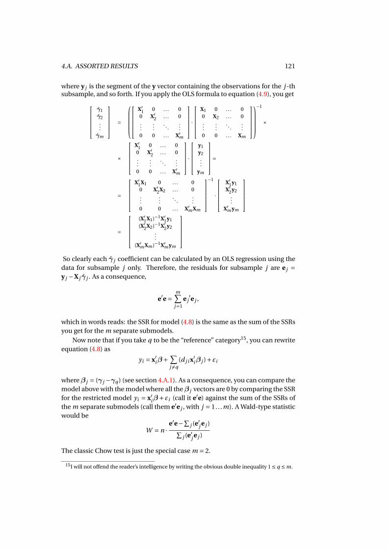
4.A. ASSORTED RESULTS 121
where y j is the segment of the y vector containing the observations for the j -thsubsample, and so forth. If you apply the OLS formula to equation (4.9), you get
γ1γ2
...γm
=
X′1 0 . . . 0
0 X′2 . . . 0
......
. . ....
0 0 . . . X′m
·
X1 0 . . . 00 X2 . . . 0...
.... . .
...0 0 . . . Xm
−1
×
×
X′
1 0 . . . 00 X′
2 . . . 0...
.... . .
...0 0 . . . X′
m
·
y1y2...
ym
=
=
X′
1X1 0 . . . 00 X′
2X2 . . . 0...
.... . .
...0 0 . . . X′
m Xm
−1
·
X′
1y1X′
2y2...
X′m ym
=
(X′
1X1)−1X′1y1
(X′2X2)−1X′
2y2...
(X′m Xm )−1X′
m ym
So clearly each γ j coefficient can be calculated by an OLS regression using the
data for subsample j only. Therefore, the residuals for subsample j are e j =y j −X j γ j . As a consequence,
e′e =m∑
j=1e j
′e j ,
which in words reads: the SSR for model (4.8) is the same as the sum of the SSRsyou get for the m separate submodels.
Now note that if you take q to be the “reference” category15, you can rewriteequation (4.8) as
yi = x′iβ+ ∑j 6=q
(d j i x′iβ j )+εi
whereβ j = (γ j −γq ) (see section 4.A.1). As a consequence, you can compare themodel above with the model where all theβ j vectors are 0 by comparing the SSRfor the restricted model yi = x′iβ+εi (call it e′e) against the sum of the SSRs ofthe m separate submodels (call them e′e j , with j = 1. . .m). A Wald-type statisticwould be
W = n ·e′e−∑
j (e′j e j )∑j (e′j e j )
The classic Chow test is just the special case m = 2.
15I will not offend the reader’s intelligence by writing the obvious double inequality 1 ≤ q ≤ m.
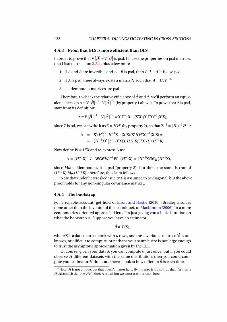
122 CHAPTER 4. DIAGNOSTIC TESTING IN CROSS-SECTIONS
4.A.3 Proof that GLS is more efficient than OLS
In order to prove that V[β
]−V[β
]is psd, I’ll use the properties on psd matrices
that I listed in section 3.A.4, plus a few more
1. if A and B are invertible and A−B is psd, then B−1 − A−1 is also psd;
2. if A is psd, there always exists a matrix H such that A = H H ′;16
3. all idempotent matrices are psd.
Therefore, to check the relative efficiency of β and β, we’ll perform an equiv-
alent check on∆≡ V[β
]−1−V[β
]−1(by property 1 above). To prove that∆ is psd,
start from its definition:
∆≡ V[β
]−1 −V[β
]−1 = X′Σ−1X− (X′X)(X′ΣX)−1(X′X);
sinceΣ is pd, we can write it asΣ= H H ′ (by property 2), so thatΣ−1 = (H ′)−1H−1:
∆ = X′(H ′)−1H−1X− (X′X)(X′H H ′X)−1(X′X) == (H−1X)′
[I −H ′X(X′H H ′X)−1X′H
](H−1X).
Now define W = H ′X and re-express ∆ as:
∆ = (H−1X)′[I −W(W′W)−1W′] (H−1X) = (H−1X)′MW(H−1X),
since MW is idempotent, it is psd (property 3); but then, the same is true of(H−1X)′MW(H−1X); therefore, the claim follows.
Note that under heteroskedasticityΣ is assumed to be diagonal, but the aboveproof holds for any non-singular covariance matrix Σ.
4.A.4 The bootstrap
For a reliable account, get hold of Efron and Hastie (2016) (Bradley Efron isnone other than the inventor of the technique), or MacKinnon (2006) for a moreeconometrics-oriented approach. Here, I’m just giving you a basic intuition onwhat the bootstrap is. Suppose you have an estimator
θ = T (X),
where X is a data matrix matrix with n rows, and the covariance matrix of θ is un-known, or difficult to compute, or perhaps your sample size is not large enoughto trust the asymptotic approximation given by the CLT.
Of course, given your data X you can compute θ just once, but if you couldobserve H different datasets with the same distribution, then you could com-pute your estimator H times and have a look at how different θ is each time.
16Note: H is not unique, but that doesn’t matter here. By the way, it is also true that if a matrixH exists such that A = H H ′, then A is psd, but we won’t use this result here.
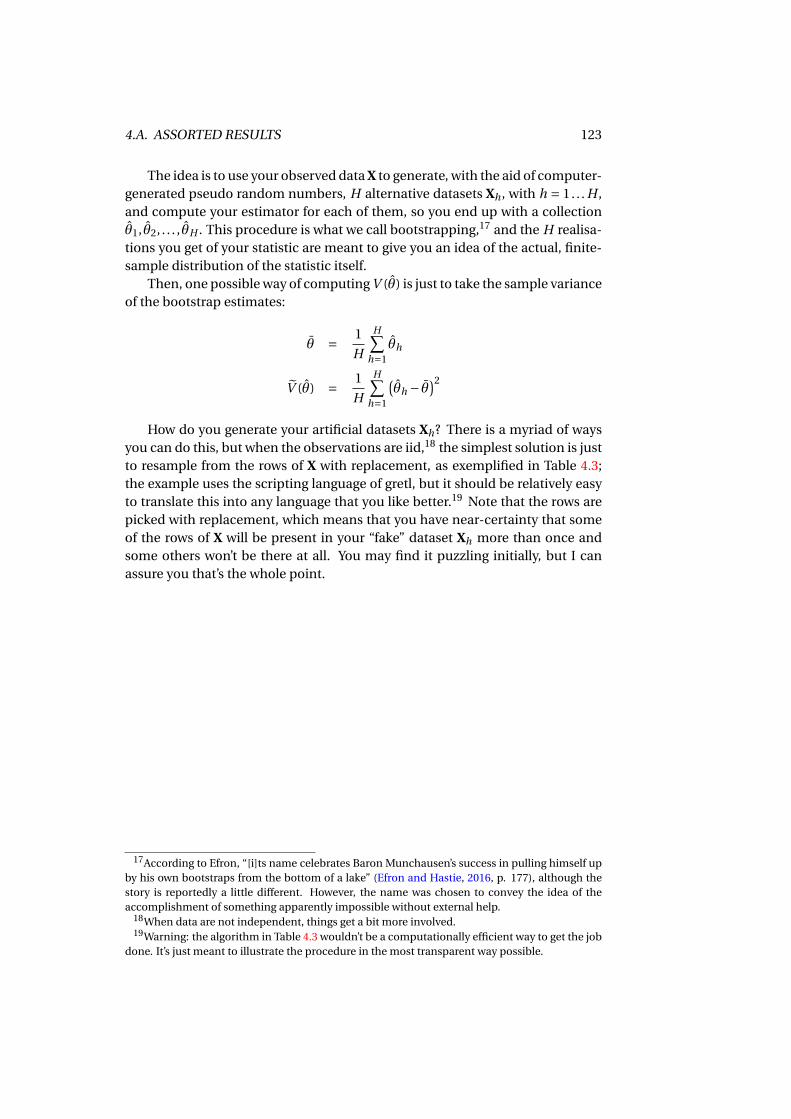
4.A. ASSORTED RESULTS 123
The idea is to use your observed data X to generate, with the aid of computer-generated pseudo random numbers, H alternative datasets Xh , with h = 1. . . H ,and compute your estimator for each of them, so you end up with a collectionθ1, θ2, . . . , θH . This procedure is what we call bootstrapping,17 and the H realisa-tions you get of your statistic are meant to give you an idea of the actual, finite-sample distribution of the statistic itself.
Then, one possible way of computing V (θ) is just to take the sample varianceof the bootstrap estimates:
θ = 1
H
H∑h=1
θh
V (θ) = 1
H
H∑h=1
(θh − θ)2
How do you generate your artificial datasets Xh? There is a myriad of waysyou can do this, but when the observations are iid,18 the simplest solution is justto resample from the rows of X with replacement, as exemplified in Table 4.3;the example uses the scripting language of gretl, but it should be relatively easyto translate this into any language that you like better.19 Note that the rows arepicked with replacement, which means that you have near-certainty that someof the rows of X will be present in your “fake” dataset Xh more than once andsome others won’t be there at all. You may find it puzzling initially, but I canassure you that’s the whole point.
17According to Efron, “[i]ts name celebrates Baron Munchausen’s success in pulling himself upby his own bootstraps from the bottom of a lake” (Efron and Hastie, 2016, p. 177), although thestory is reportedly a little different. However, the name was chosen to convey the idea of theaccomplishment of something apparently impossible without external help.
18When data are not independent, things get a bit more involved.19Warning: the algorithm in Table 4.3 wouldn’t be a computationally efficient way to get the job
done. It’s just meant to illustrate the procedure in the most transparent way possible.
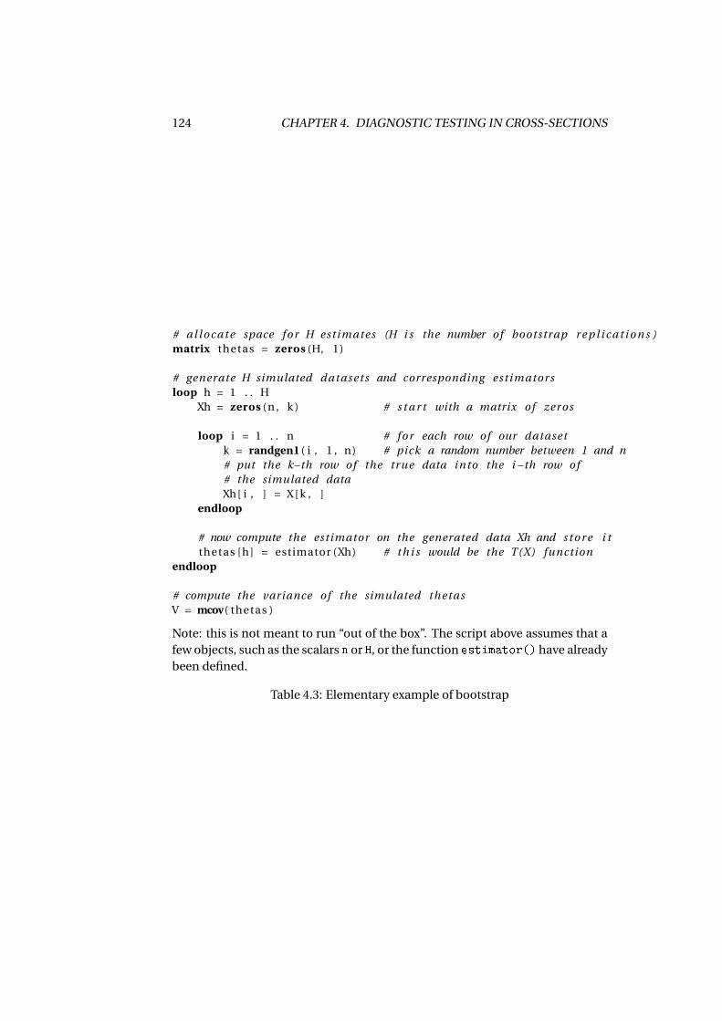
124 CHAPTER 4. DIAGNOSTIC TESTING IN CROSS-SECTIONS
# a l l o c a t e space f o r H estimates (H i s the number of bootstrap r e p l i c a t i o n s )matrix thetas = zeros (H, 1)
# generate H simulated datasets and corresponding estimatorsloop h = 1 . . H
Xh = zeros (n , k ) # s t a r t with a matrix of zeros
loop i = 1 . . n # f o r each row of our datasetk = randgen1 ( i , 1 , n) # pick a random number between 1 and n# put the k−th row of the true data into the i −th row of# the simulated dataXh[ i , ] = X[ k , ]
endloop
# now compute the estimator on the generated data Xh and s t o r e i tthetas [h] = estimator (Xh) # t h i s would be the T(X) function
endloop
# compute the variance of the simulated thetasV = mcov( thetas )
Note: this is not meant to run “out of the box”. The script above assumes that afew objects, such as the scalars n or H, or the function estimator() have alreadybeen defined.
Table 4.3: Elementary example of bootstrap
Chapter 5
Dynamic Models
5.1 Dynamic regression
In cross sectional datasets, it is quite natural to assume that the most useful in-formation set on which to condition the distribution of yi is xi . Why should weconsider, for the conditional distribution of yi , the information available for in-dividual j as relevant (with i 6= j )? In some cases, there could be something tothis; perhaps individuals i and j have some unobservable feature in common,but in most cross-sectional datasets this shouldn’t be something to worry about.
This argument does not apply to time-series datasets. Here, we have twofundamental differences from cross-sectional datasets:
1. Data have a natural ordering.
2. At any given point in time, we can take as known what happened in thepast (and, possibly, at present time), but the future remains unknown.
This means that, if we want to condition yt to something1, we may proceedas in chapter 3 and consider E
[yt |xt
], but this is unlikely to be a good idea, es-
pecially in the light of a feature that most economics time series display, that is,they are very persistent.
Persistence is a loose term we use for describing the quality, that time se-ries often possess, whereby contiguous observations look more like each otherthan distant ones. In other words, persistence is the observable consequence ofthe fact that most phenomena evolve gradually through time.2 In fact, you maythink of time series as something with “memory” of the past. The informationembodied in a time series dataset is not only in the numbers it contains, but
1Attention: for this chapter, I’m going to switch to a slightly different notation convention thanwhat I used in the previous chapters. Since we’re dealing with time series, I will use the symbols tand T instead of i and n, so for example the dependent variable has values y1, . . . , yt , . . . , yT .
2In fact, the econometric treatment of time series data has become, since the 1980s, such avast and complex subject that we may legitimately treat time-series econometrics as a relativelyautonomous scientific field (with financial econometrics as a notable sub-field).
125
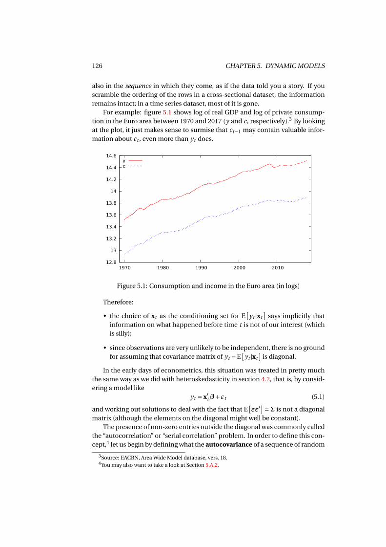
126 CHAPTER 5. DYNAMIC MODELS
also in the sequence in which they come, as if the data told you a story. If youscramble the ordering of the rows in a cross-sectional dataset, the informationremains intact; in a time series dataset, most of it is gone.
For example: figure 5.1 shows log of real GDP and log of private consump-tion in the Euro area between 1970 and 2017 (y and c, respectively).3 By lookingat the plot, it just makes sense to surmise that ct−1 may contain valuable infor-mation about ct , even more than yt does.
12.8
13
13.2
13.4
13.6
13.8
14
14.2
14.4
14.6
1970 1980 1990 2000 2010
yc
Figure 5.1: Consumption and income in the Euro area (in logs)
Therefore:
• the choice of xt as the conditioning set for E[
yt |xt]
says implicitly thatinformation on what happened before time t is not of our interest (whichis silly);
• since observations are very unlikely to be independent, there is no groundfor assuming that covariance matrix of yt −E
[yt |xt
]is diagonal.
In the early days of econometrics, this situation was treated in pretty muchthe same way as we did with heteroskedasticity in section 4.2, that is, by consid-ering a model like
yt = x′tβ+εt (5.1)
and working out solutions to deal with the fact that E[εε′
]=Σ is not a diagonalmatrix (although the elements on the diagonal might well be constant).
The presence of non-zero entries outside the diagonal was commonly calledthe “autocorrelation” or “serial correlation” problem. In order to define this con-cept,4 let us begin by defining what the autocovariance of a sequence of random
3Source: EACBN, Area Wide Model database, vers. 18.4You may also want to take a look at Section 5.A.2.
5.1. DYNAMIC REGRESSION 127
variables is: suppose you have T random variables observed through time
z1, z2, . . . , zt , . . . , zT .
The covariance between zt and zs is an autocovariance, since it’s the covarianceof a random variable “with itself at a different time”, so to speak. Clearly, if thisquantity is different from 0, the two random variables zt and zs cannot be inde-pendent. If we standardise this covariance as
ρt ,s = Cov[zs , zt ]pV[zt ]V[zs]
we have something called autocorrelation. In most cases, it makes sense to as-sume that the correlation between zs and zt is only a function of how far theyare from each other; that is, assume that ρt ,s is just a function of |t − s|; if this isthe case, the quantity Corr[zt−1, zt ] = Corr[zt , zt+1] = . . . is called first-order au-tocorrelation or autocorrelation of order 1. Generalisation is straightforward.
Clearly, if the autocorrelation between εt and εs is nonzero for some t and s,Σ cannot be diagonal, so GLS solutions have been devised5, and a clever gener-alisation of White’s robust estimator (due to Whitney Newey and Kenneth West)is also available, but instead of “fixing” OLS, a much better strategy is to rethinkour conditioning strategy. That is, instead of devising clever ways to perform ac-ceptable inference on equation (5.1), we’d be much better off if we redefined ourobject of interest.
What we want to do is using all the possibly relevant available informationas our conditioning set; to this end, define the information set at time t as6
ℑt =
x1,x2, . . .xt , y1, y2, . . . , yt−1
;
for example, in order to build a model where consumption is the dependentvariable and the only explanatory variable is income (a dynamic consumptionfunction, if you will), it may make sense to condition consumption on the wholeinformation set ℑt .
Therefore, the conditioning operation will be done by using all the variablesrelevant for the distribution of yt that can be assumed to be known at that time.Clearly, that includes the current value of xt , but also the past of both yt and xt .Possibly, even future variables that are known with certainty at time t ; variablessuch as these are normally said to be deterministic. Apart from the constantterm (xt = 1), popular examples include time trends (eg xt = t ), seasonal dummy
5For the readers who are into the history of econometrics: the so-called Cochrane-Orcutt es-timator and its refinements are totally forgotten today, but they were a big thing back in the 1960sand 1970s.
6To be rigorous, we should define the information set by using a technical tool called a σ-field. This ensures that ℑt contains all possible functions of the elements listed above (∆yt−1, forexample). But in an introductory treatment such as this, I’ll just use the reader’s intuition and useℑt as “all the things we knows at time t”.
128 CHAPTER 5. DYNAMIC MODELS
variables (eg xt = 1 if t is the month of May), or more exotic choices, such as thenumber of days in a given month, that is known in advance. Note that (this willbe very important) ℑt is an element of a sequence where ℑt−1 ⊆ ℑt ⊆ ℑt+1; inother words, the sequence of informations sets is increasing.7
Now consider the conditional expectation E[
yt |ℑt]; even under the linearity
assumption, this object may have two potentially troublesome characteristics:
1. since the sequence ℑt is increasing, E[
yt |ℑt]
may contain informationthat goes indefinitely back into the past, and
2. E[
yt |ℑt]
could be different for each t .
If none of the above is true, things are much simplified; under the additionalassumption of linearity of the conditional mean,
E[
yt |ℑt]= p∑
i=1αi yt−i +
q∑i=0β′
i xt−i ,
where p and q are finite numbers. Although in principle ℑt contains all the past,no matter how remote, only the most recent elements of ℑt actually enter theconditional expectation. A slightly more technical way of expressing the sameconcept is: we are assuming that there is a subset of ℑt (call it Ft ), that containsonly recent information, such that conditioning on ℑt or Ft makes no differ-ence:
E[
yt |ℑt]= E
[yt |Ft
], (5.2)
where ℑt ⊃Ft . In practice, Ft is the relevant information at time t .The linearity assumption makes the regression function of yt on ℑt a differ-
ence equation, that is, a relationship in which an element of a sequence yt isdetermined by a linear combination of its own past and the present and past ofanother sequence xt ;8 if we proceed in a similar way as in chapter 3, and defineεt ≡ yt −E
[yt |ℑt
], we can write the so-called ADL model:
yt =p∑
i=1αi yt−i +
q∑i=0β′
i xt−i +εt . (5.3)
The ADL acronym is for Autoregressive Distributed Lags (some people prefer theARDL acronym): in many cases, we call the above an ADL(p, q) model, to makeit explicit that the conditional mean contains p lags of the dependent variableand q lags of the explanatory variables.
Of course, it would be very nice if we could estimate the above parametersvia OLS. Clearly, the first few observations would have to be discarded, but once
7Or, if you will, we are assuming that we always learn and never forget.8Note: this definition works for our present purposes, but in some cases you may want to con-
sider non-linear relationships, or cases which involve future values.
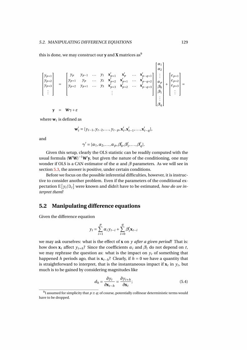
5.2. MANIPULATING DIFFERENCE EQUATIONS 129
this is done, we may construct our y and X matrices as9
yp+1
yp+2
yp+3...
=
yp yp−1 . . . y1 x′p+1 x′p . . . x′p−q+1
yp+1 yp . . . y2 x′p+2 x′p+1 . . . x′p−q+2
yp+2 yp+1 . . . y3 x′p+3 x′p+2 . . . x′p−q+3...
α1
α2...αp
β0
β1...βq
+
εp+1
εp+2
εp+3...
=
y = Wγ+ε
where wt is defined as
w′t = [yt−1, yt−2, . . . , yt−p ,x′t ,x′t−1, . . . ,x′t−q ],
andγ ′ = [α1,α2, . . . ,αp ,β′
0,β′1, . . . ,β′
q ].
Given this setup, clearly the OLS statistic can be readily computed with theusual formula (W′W)−1W′y, but given the nature of the conditioning, one maywonder if OLS is a CAN estimator of the α and β parameters. As we will see insection 5.3, the answer is positive, under certain conditions.
Before we focus on the possible inferential difficulties, however, it is instruc-tive to consider another problem. Even if the parameters of the conditional ex-pectation E
[yt |ℑt
]were known and didn’t have to be estimated, how do we in-
terpret them?
5.2 Manipulating difference equations
Given the difference equation
yt =p∑
i=1αi yt−i +
q∑i=0β′
i xt−i
we may ask ourselves: what is the effect of x on y after a given period? That is:how does xt affect yt+h? Since the coefficients αi and βi do not depend on t ,we may rephrase the question as: what is the impact on yt of something thathappened h periods ago, that is xt−h? Clearly, if h = 0 we have a quantity thatis straightforward to interpret, that is the instantaneous impact if xt in yt , butmuch is to be gained by considering magnitudes like
dh = ∂yt
∂xt−h= ∂yt+h
∂xt; (5.4)
9I assumed for simplicity that p ≥ q ; of course, potentially collinear deterministic terms wouldhave to be dropped.
130 CHAPTER 5. DYNAMIC MODELS
the dh parameters take the name of dynamic multipliers, or just multipliers forshort. In order to find a practical and general way to compute them, we will needa few extra tools. Read on.
5.2.1 The lag operator
Time series are nothing but sequences of numbers, with a natural ordering givenby time. In many cases, we may want to manipulate sequences by means ofappropriate operators. The lag operator is generally denoted by the letter L byeconometricians (statisticians prefer B — savages!); it’s an operator that turnsa sequence xt into another sequence, that contains the same objects as xt , butshifted back by one period.10 If you apply L to a constant, the result is the sameconstant. In formulae,
Lxt = xt−1
Repeated application of the L operator n times is indicated by Ln , and thereforeLn xt = xt−n . By convention, L0 = 1. The L operator is linear, which means that,if a and b are constant, then L(axt + b) = aLxt + b = axt−1 + b. These simpleproperties have the nice consequence that, in many cases, we can manipulatethe L operator algebraically as if it was a number. This trick is especially usefulwhen dealing with polynomials in L. Allow me to exemplify:
Example 5.1Call bt the money you have at time t , and st the difference between the moneyyou earn and the money you spend between t − 1 and t (in other words, yoursavings). Of course,
bt = bt−1 + st .
Now the same thing with the lag operator::
bt = Lbt + st → bt −Lbt = (1−L)bt =∆bt = st
The∆ operator, which I suppose not unknown to the reader, is defined as (1−L),that is a polynomial in L of degree 1. The above expression simply says that thevariation in the money you have is your net saving.
Example 5.2Call qt the GDP for the Kingdom of Verduria in quarter t . Obviously, yearly GDPis given by
yt = qt +qt−1 +qt−2 +qt−3 = (1+L+L2 +L3)qt
10In certain cases, you might want to use the lead operator, usually notated as F , which is de-fined as the inverse to the lag operator (F xt = xt+1, or F = L−1). I’m not using it in this book, butits usage is very common in economic models with rational expectations.
5.2. MANIPULATING DIFFERENCE EQUATIONS 131
Since (1+x +x2 +x3)(1−x) = (1−x4), if you “multiply” the equation above11 by(1−L) you get
∆yt = (1−L4)qt = qt −qt−4;
The variation in yearly GDP between quarters is just the difference between thequarterly figures a year apart from each other.
A polynomial P (x) may be evaluated at any value, but two cases are of specialinterest. Obviously, if you evaluate P (x) for x = 0 you get the “constant” coeffi-cient of the polynomial, since P (0) = p0 +p1 ·0+p2 ·0+·· · = p0; instead, if youevaluate P (1) you get the sum of the polynomial coefficients:
P (1) =n∑
j=0p j 1 j =
n∑j=0
p j .
This turns out to be quite handy when you apply a lag polynomial to a constant,since
P (L)µ=n∑
j=0p jµ=µ
n∑j=0
p j = P (1)µ.
There are two more routine results that come in very handy: the first one hasto do with inverting polynomials of order 1. It can be proven that, if |α| < 1,
(1−αL)−1 = (1+αL+α2L2 +·· · ) =∞∑
i=0αi Li ; (5.5)
the other one is that a polynomial P (x) is invertible if and only if all its roots aregreater than one in absolute value:
1
P (x)exists iff P (x) = 0 ⇒|x| > 1. (5.6)
The proofs are in subsection 5.A.1.
Example 5.3 (The Keynesian multiplier)Let me illustrate a possible use of polynomial manipulation by a very old-schoolmacro example: the simplest possible version of the Keynesian multiplier idea.Suppose that
Yt = Ct + It ; (5.7)
Ct = αYt−1; (5.8)
where Yt id GDP, Ct is aggregate consumption and It is investment; 0 <α< 1 isthe marginal propensity to consume.
11To be precise, we should say: ‘if you apply the (1−L) operator to the expression above’.
132 CHAPTER 5. DYNAMIC MODELS
By combining the two equations,
Yt =αYt−1 + It → (1−αL)Yt = It .
therefore, by applying the first degree polynomial A(L) = (1−αL) to the Yt se-quence (national income), you get the time series for investments, simply be-cause It = Yt −Ct = Yt −αYt−1.
If you now invert the A(L) = (1−αL) operator,
Yt = (1+αL+α2L2 +·· · )It =∞∑
i=0αi It−i :
aggregate demand at time t can be seen as a weighted sum of past and presentinvestment. Suppose that investment goes from 0 to 1 at time 0. This bringsabout a unit increase in GDP via equation (5.7); but then, at time 1 consumptiongoes up by α, by force of equation (5.8), so at time 2 it increases byα2 and so on.Since 0 <α< 1, the effect dies out eventually.
If investments were constant through time, then It = I and the expressionabove becomes the familiar “Keynesian multiplier” formula:
Yt = I∞∑
i=0αi = I
1−α .
A word of caution: in many cases, it’s OK to manipulate L algebraically as ifit was a number, but sometimes it’s not: the reader should always keep in mindthat the expression Lxt does not mean ‘L times xt ’, but ‘L applied to xt ’. Thefollowing example should, hopefully, convince you.
Example 5.4Given two sequence xt and yt , define the sequence zt as zt = xt · yt . Obviously,zt−1 = xt−1 yt−1; however, one may be tempted to argue that
zt−1 = xt−1 yt−1 = Lxt Lyt = L2xt yt = L2zt = zt−2
which is obviously absurd.
5.2.2 Dynamic multipliers
Manipulating polynomials in L is the technical tool we need in order to handlethe problem that we are ultimately after. Let’s start from a difference equationlike the following:
A(L)yt = B(L)xt
5.2. MANIPULATING DIFFERENCE EQUATIONS 133
where the degrees of the A(L) and B(L) polynomials are p and q , respectively. Ifthe polynomial A(L) is invertible, the difference equation is said to be stable. Inthis case, we may define D(L) = A(L)−1B(L) = B(L)/A(L); in general, D(L) maynot be of finite order, so
yt = D(L)xt =∞∑
i=0di xt−i
This is all we need for dealing with the issue we started from, that is: howdo we interpret the parameters of a dynamic model? The answer is easy if youconsider that the dynamic multipliers as defined in equation (5.4),
di = ∂yt
∂xt−i= ∂yt+i
∂xt,
are simply the coefficients of the D(L) polynomial.12 It is possible to calculatethem analytically by inverting the A(L) polynomial, but doing so is neither in-structive nor enjoyable. On the contrary, the same effect can be achieved byusing a nice recursive algorithm.
The impact multiplier d0 is easy to find, since d0 = D(0) = B(0)/A(0), whichsimply equals β0 (since A(0) = 1). All other multipliers can be found by means of(5.4), which can be used to express di in terms of di−1,di−2 etc. Once you haved0, the rest of the sequence follows. Let me show you a practical example. Foran ADL(1,1) model,
yt =αyt−1 +β0xt +β1xt−1, (5.9)
use the definition of a multiplier as a derivative and write
d0 = ∂yt
∂xt= ∂
∂xt
(αyt−1 +β0xt +β1xt−1
)=β0
d1 = ∂yt
∂xt−1= ∂
∂xt−1
(αyt−1 +β0xt +β1xt−1
)=α∂yt−1
∂xt−1+β1 =αd0 +β1,
where we used the property
∂yt−1
∂xt−1= ∂yt
∂xt= d0
in such a way that d1 is expressed as a function of d0; similarly,
d2 = ∂yt
∂xt−2= ∂
∂xt−2
(αyt−1 +β0xt +β1xt−1
)=α∂yt−1
∂xt−2=αd1
and so on, and on, and on, . . .
12As we will see in section 5.3, invertibility of A(L) is not only required for the calculation of themultipliers, but also for the CAN property of OLS.
134 CHAPTER 5. DYNAMIC MODELS
A nice and cool way to express the above is by saying that the multipliers canbe calculated through a difference equation with the same polynomials as theoriginal one; the sequence of multipliers obeys the relationship
A(L)di = B(L)ui , (5.10)
where ui is a sequence that contains 1 for u0, and 0 everywhere else. This makesit easy to calculate the multipliers numerically, given the polynomial coefficients,via appropriate software.
Example 5.5 (Inversion of polynomials)Take for example the following difference equation:
yt = 0.2yt−1 +0.4xt +0.3xt−2.
In this case, A(L) = 1−0.2L and B(L) = 0.4+0.3L2. The inverse of A(L) is
A(L)−1 = 1+0.2L+0.04L2 +0.008L3 +·· · =∞∑
i=00.2i Li ;
therefore,
B(L)
A(L)= (0.4+0.3L2)× (1+0.2L+0.04L2 +0.008L3 +·· · ).
The two polynomials can be multiplied directly, as in
B(L)
A(L)= 0.4× (1+0.2L+0.04L2 +0.008L3 +·· · )+
+0.3L2 × (1+0.2L+0.04L2 +0.008L3 +·· · ) == 0.4+0.08L+0.016L2 +0.0032L3 +·· ·+
+0.3L2 +0.06L3 +0.012L4 +0.0024L5 · · · == 0.4+0.08L+0.316L2 +0.0632L3 +·· ·
but it’s really boring. The recursive way of calculating the coefficient is muchquicker:
d0 = B(0)/A(0) = 0.4/1 = 0.4
d1 = 0.2 ·d0 = 0.08
d2 = 0.2 ·d1 +0.03 = 0.016+0.3 = 0.316
d3 = 0.2 ·d2 = 0.0632
and so on.
5.2. MANIPULATING DIFFERENCE EQUATIONS 135
5.2.3 Interim and long-run multipliers
If you go back to the definition of the multipliers, (5.4), that is di = ∂yt
∂xt−i= ∂yt+i
∂xt,
it is quite natural to interpret the magnitude dh as the effect of something thathappened h periods ago on what we see today. The implicit idea in this defini-tion is that the source of the dynamic behaviour in our system is a one-off event.
In many cases, instead, we could be interested in computing the effect onyt of a permanent change in xt . Clearly, at time 0 the effect will be equal to theimpact multiplier d0, but after one period the instantaneous effect will overlapwith the lagged one, so the effect will be equal to d0 +d1. By induction, we maydefine a new sequence of multipliers as
c j = d0 +d1 +·· ·+d j =j∑
i=0di . (5.11)
These are called interim multipliers and measure the effect on yt of a perma-nent change in xt that took place j periods ago. In order to see what happens inthe long run after a permanent change, we may also want to consider the long-run multiplier c = lim j→∞ c j . Calculating c is much easier than what may seem,since
c j =∞∑
i=0di = D(1);
that is: c is the number you get by evaluating the polynomial D(z) in z = 1; sinceD(z) = B(z)/A(z), c can be easily computed as c = D(1) = B(1)
A(1) .
Example 5.6 (interim multipliers)Let’s go back to the difference equation we used in example 5.5:
yt = 0.2yt−1 +0.4xt +0.3xt−2.
Interim multipliers are easily computed:
c0 = d0 = 0.4
c1 = d0 +d1 = c0 +d1 = 0.48
c2 = d0 +d1 +d2 = c1 +d2 = 0.796
and so on. The limit of this sequence (the long-run multiplier) is also easy tocompute:
c = D(1) = B(1)
A(1)= 0.7/0.8 = 0.875
Et voilà.
The long-run multiplier c is very important, because tells us what the pro-portion is between yt and xt in steady state: imagine we fix xt at a certain value
136 CHAPTER 5. DYNAMIC MODELS
that stays the same forever. Is there a limit value for yt ? It can be shown that thelimit exists as long as the difference equation is stable; if this condition is met,then the system admits a steady state. The steady state is a long-run equilib-rium: in steady state, neither yt nor xt change until external shocks come fromoutside the system to perturb it.
Imagine that the system is in steady state: both variables are time-invariant,so yt = Y and xt = X ; as a consequence,
A(L)yt = B(L)xt ⇒ A(L)Y = B(L)X ⇒ A(1)Y = B(1)X ⇒ Y = B(1)
A(1)X = c X
so the system is not in equilibrium any time yt 6= cxt . As we will see, this trivialobservation will become important later.
5.3 Inference on OLS with time-series data
At this point, we know how to interpret the coefficients of a difference equation.An ADL model (equation (5.3), reproduced here for the reader’s convenience)
A(L)yt = B(L)xt +εt
is basically a difference equation plus an error term; therefore, the coefficientsof the two polynomials A(L) and B(L) are unobservable, but perhaps we couldfind a CAN estimator.
We showed in section 5.1 how OLS can be applied to a dynamic model bydefining the X matrix and the y vector appropriately. The question now is: isOLS a CAN estimator of the ADL parameters? The answer is positive, if certainconditions are satisfied.
5.3.1 Martingale differences
Define wt like at the end of section 5.1, as
w′t = [yt−1, yt−2, . . . , yt−p ,x′t ,x′t−1, . . . ,x′t−q ],
so that we can write our dynamic model as
yt = w′tγ+εt
where of course γ ′ = [α1,α2, . . . ,αp ,β′0,β′
1, . . . ,β′q ].
The first important requirement is that the second moments of wt exist andthat
T −1T∑
t=1wt w′
tp−→Q
where Q is invertible. The conditions under which we can expect this to happenare quite tricky to lay down formally. Here, I’ll just say that in order for every-thing to work as expected, it is sufficient that our observed data are realisations
5.3. INFERENCE ON OLS WITH TIME-SERIES DATA 137
of covariance-stationary and ergodic stochastic processes.13 For a summary de-scription of what this means, I have written subsection 5.A.2 at the end of thischapter. If you can’t be bothered, just take this to mean that all moments up tothe fourth order of all the observables exist and are stable through time.
On top of this, a fundamental ingredient for OLS being a CAN estimator ofthe parameters in equation (5.3) is that εt be a martingale difference sequence(or MDS for short).14
Roughly speaking, a MDS is a sequence of random variables whose expectedvalue (conditional to a certain information set) meets certain requirements:
• a martingale with respect to ℑt−1 is a sequence of random variables X t
such that E[X t |ℑt−1] = X t−1;
• If X t is a martingale, then ∆X t is a MDS: E[∆X t |ℑt−1] = 0
Of course, if we could condition yt on ℑt then εt would be a MDS by con-struction:
E[εt |ℑt ] = E[
yt −E[
yt |ℑt] |ℑt
]= E[
yt |ℑt]−E
[yt |ℑt
]= 0
(this is essentially the same argument we used in section 3.1). But of course wecan’t use ℑt in practice; however, we’re assuming (see equation 5.2) that thereexists a subset Ft ⊂ ℑt such that E
[yt |ℑt
] = E[
yt |Ft], so Ft (which is usable,
because it’s finite) is just as good. So if you condition yt on Ft , the quantityεt = yt −E
[yt |Ft
]is a MDS and all is well.
However, what happens if you use a conditioning set Gt that is “too small”?That is, that doesn’t contain Ft ? In that case, the difference ut = yt −E
[yt |Gt
]is
not a MDS with respect to ℑt : if E[
yt |Gt] 6= E
[yt |Ft
], then
E[ut |ℑt ] = E[
yt −E[
yt |Gt] |ℑt
]= E[
yt |Ft]−E
[yt |Gt
] 6= 0.
On the contrary, it is easy to prove that in the opposite case, when you conditionon a subset of ℑt that is larger than Ft , no problems arise.
This remark is extremely important in practice because the order of the poly-nomials A(L) and B(L) (p and q , respectively) are not known: what happens ifwe get them wrong? Well, if they are larger than the “true” ones, then our con-ditioning set contains Ft , and all is well. But if they’re smaller, the disturbanceterm of our model is not a MDS, and all inference collapses. For example, ifp = 2 and q = 3, then Ft contains yt−1, yt−2, xt , xt−1, xt−2 and xt−3. Any set ofregressors that doesn’t include at least these renders inference invalid.
13I’m being very vague and unspecific here: if you want an authoritative source on the asymp-totics for dynamic models, you’ll want to check chapters 6 and 7 in Davidson (2000).
14MDSs arise quite naturally in inter-temporal optimisation problems, so their usage in eco-nomic and finance models with uncertainty is very common. In this contexts, an MDS is, so tospeak, something that cannot be predicted in any way from the past. For a thorough discussion,see Hansen and Sargent (2013), chapter 2.
138 CHAPTER 5. DYNAMIC MODELS
Therefore, εt is a MDS, if we pick p and q large enough. The obvious impli-cation is that E[εt |wt ] = 0 (since wt is contained in ℑt−1). If we also add a ho-moskedasticity assumption E
[ε2
t |wt]=σ2, then we have a set of results that par-
allel completely those in section 3.2. To put it simply, everything works exactlythe same way as in cross-sectional models: the martingale property ensures that
E[wt ·εt |ℑt ] = 0, and therefore γp−→γ; additionally,
pT (γ−γ)
d−→ N(0,σ2Q−1)
In practice, the whole testing apparatus we set up for cross sectional datasetsremains valid; the t statistic, the W statistic, everything. Nice, isn’t it? In addi-tion, since the dynamic multipliers are continuous and differentiable functionsof the ADL parameters γ, we can simply compute the multipliers from the esti-mated parameters γ and get automatically CAN estimators of the multipliers.15
The homoskedasticity assumption is not nor-mally a problem, except for financial data athigh frequencies (eg daily); for those cases, youget a separate class of models, the most no-table example of which is the so-called GARCH
model, which I will not consider here, but areextremely important in the field of financialeconometrics. In case we want to stick withOLS, robust estimation is perfectly viable.
5.3.2 Testing for autocorrelation and the general-to-specific approach
Basically, we need a test for deciding, on the basis of the OLS residuals, whetherεt is a MDS or not. Because if it were not, the OLS estimator would not be con-sistent for the ADL parameters, let alone have the asymptotic distribution werequire for carrying out tests. As I argued in the previous section, εt cannot be aMDS if we estimate a model in which the orders p and q that we use for the twopolynomials A(L) and B(L) are too small.
Most tests hinge on the fact that a MDS cannot be autocorrelated:16 for thesake of brevity, I don’t prove this here, but the issue is discussed in section 5.A.3if you’re interested. Therefore, in practice, the most important diagnostic checkon a dynamic regression model is checking for autocorrelation: if we reject thenull of no autocorrelation, then εt cannot be a MDS.
All econometric software pays tribute to tradition by reporting a statistic in-vented by James Durbin and Geoffrey Watson in 1950, called DW statistic in theirhonour. Its support is, by construction, the interval between 0 and 4, and ide-ally it should be close to 2. It is practically useless, because it only checks forautocorrelation of order 1, and there are several cases in which it doesn’t work
15Unfortunately, the function linking multipliers and parameters is nonlinear, so you need thedelta method to compute their asymptotic variance. See section 2.3.2.
16If I were insufferably pedantic, I would say “a MDS with finite second moments”.
5.3. INFERENCE ON OLS WITH TIME-SERIES DATA 139
(notably, when lags of the dependent variable are among the regressors); there-fore, nobody uses it anymore, although all software packages routinely print itout as a homage to tradition.
The Godfrey test (also known as the Breusch-Godfrey test, or the LM test forautocorrelation) is much better:
A(L)yt = B(L)xt +γ1et−1 +γ2et−2 +·· ·+γhet−h +εt
where et is the t-th OLS residual and h is known as the order of the test. Thereis no precise rule for choosing h; the most important aspect to consider is “howlong is the period we can reasonably expect to consider long enough for dynamiceffects to show up?”. When dealing with macro time series, a common choice is2 years. That is, it is tacitly assumed that nothing can happen now, provoke noeffects for two years, and then suddenly do something.17 Therefore, you woulduse h = 2 for yearly data, h = 8 for quarterly data, and so on. But clearly, this is avery subjective criterion, so take it with a pinch of salt and be ready to adjust itto your particular dataset.
This test, being a variable addition test, is typically implemented as an LMtest (see section 3.6.1) and is asymptotically distributed (under H0) as χ2
h . Inpractice, you carry out an auxiliary regression of the OLS residuals et against wt
and h lags of et ; you multiply R2 by T and you’re done.The Godfrey test is the cornerstone of the so-called general-to-specific esti-
mation strategy: since the polynomial orders p and q are not known in practice,one has to make a guess. There are three possible situations:
1. your guess is exactly right; you’re a lucky bastard.
2. Your guess is wrong because you overestimated p and/or q : in this case,your model contains the “true” one and the disturbance term will still be aMDS; hence, the probability of the Godfrey test rejecting the null hypoth-esis is 5%. The only slight inconvenience is that you’re using too many pa-rameters. This is not a problem, however, because asymptotic inference isvalid and you can trim your model down by using ordinary specificationtests (see section 3.3).
3. Your guess is wrong because you underestimated one of p and q : yourmodel does not contain the “true” one and the disturbance term will notbe a MDS. In this case, the Godfrey test should reject the null.
So the idea of the general-to-specific approach is: start from a large model,possibly ridiculously oversized. Then you can start refining it by ordinary hy-pothesis tests, running diagnostics18 at each step to make sure your reductionwas not too aggressive.
17“Mi ha detto mio cuggino che sa un colpo segreto. . . ”, EELST.18The most important test to run at this stage is of course the Godfrey test, but other diagnostics,
such as the RESET test for example, won’t hurt.
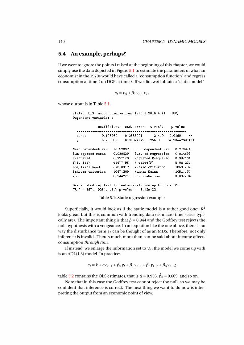
140 CHAPTER 5. DYNAMIC MODELS
5.4 An example, perhaps?
If we were to ignore the points I raised at the beginning of this chapter, we couldsimply use the data depicted in Figure 5.1 to estimate the parameters of what aneconomist in the 1970s would have called a “consumption function” and regressconsumption at time t on DGP at time t . If we did, we’d obtain a “static model”
ct =β0 +β1 yt +εt ,
whose output is in Table 5.1.
static: OLS, using observations 1970:1-2016:4 (T = 188)
Dependent variable: c
coefficient std. error t-ratio p-value
---------------------------------------------------------
const -0.128464 0.0533021 -2.410 0.0169 **
y 0.968085 0.00377749 256.3 4.98e-239 ***
Mean dependent var 13.52892 S.D. dependent var 0.273974
Sum squared resid 0.039639 S.E. of regression 0.014598
R-squared 0.997176 Adjusted R-squared 0.997161
F(1, 186) 65677.98 P-value(F) 5.0e-239
Log-likelihood 528.8912 Akaike criterion -1053.782
Schwarz criterion -1047.309 Hannan-Quinn -1051.160
rho 0.944271 Durbin-Watson 0.097794
Breusch-Godfrey test for autocorrelation up to order 8:
TR^2 = 167.119254, with p-value = 5.18e-32
Table 5.1: Static regression example
Superficially, it would look as if the static model is a rather good one: R2
looks great, but this is common with trending data (as macro time series typi-cally are). The important thing is that ρ = 0.944 and the Godfrey test rejects thenull hypothesis with a vengeance. In an equation like the one above, there is noway the disturbance term εt can be thought of as an MDS. Therefore, not onlyinference is invalid. There’s much more than can be said about income affectsconsumption through time.
If instead, we enlarge the information set to ℑt , the model we come up withis an ADL(1,3) model. In practice:
ct ' k +αct−1 +β0 yt +β1 yt−1 +β2 yt−2 +β3 yt−3;
table 5.2 contains the OLS estimates, that is α= 0.956, β0 = 0.609, and so on.
Note that in this case the Godfrey test cannot reject the null, so we may beconfident that inference is correct. The next thing we want to do now is inter-preting the output from an economic point of view.
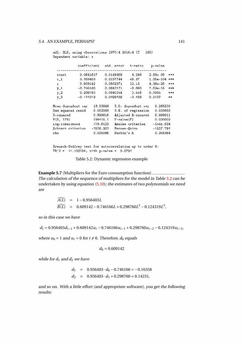
5.4. AN EXAMPLE, PERHAPS? 141
adl: OLS, using observations 1970:4-2016:4 (T = 185)
Dependent variable: c
coefficient std. error t-ratio p-value
---------------------------------------------------------
const 0.0641617 0.0149459 4.293 2.88e-05 ***
c_1 0.956403 0.0197744 48.37 1.05e-104 ***
y 0.609142 0.0502371 12.13 4.36e-25 ***
y_1 -0.746166 0.0842171 -8.860 7.82e-16 ***
y_2 0.298760 0.0840154 3.556 0.0005 ***
y_3 -0.124319 0.0499439 -2.489 0.0137 **
Mean dependent var 13.53849 S.D. dependent var 0.265530
Sum squared resid 0.002388 S.E. of regression 0.003653
R-squared 0.999816 Adjusted R-squared 0.999811
F(5, 179) 194416.1 P-value(F) 0.000000
Log-likelihood 778.8122 Akaike criterion -1545.624
Schwarz criterion -1526.302 Hannan-Quinn -1537.794
rho 0.026086 Durbin's h 0.368384
Breusch-Godfrey test for autocorrelation up to order 8:
TR^2 = 14.103154, with p-value = 0.0791
Table 5.2: Dynamic regression example
Example 5.7 (Multipliers for the Euro consumption function)The calculation of the sequence of multipliers for the model in Table 5.2 can beundertaken by using equation (5.10); the estimates of two polynomials we needare
A(L) = 1−0.956403LB(L) = 0.609142−0.746166L+0.298760L2 −0.124319L3,
so in this case we have
di = 0.956403di−1 +0.609142ui −0.746166ui−1 +0.298760ui−2 −0.124319ui−3,
where u0 = 1 and ui = 0 for i 6= 0. Therefore, d0 equals
d0 = 0.609142
while for d1 and d2 we have
d1 = 0.956403 ·d0 −0.746166 =−0.16358
d2 = 0.956403 ·d1 +0.298760 = 0.14231,
and so on. With a little effort (and appropriate software), you get the followingresults:

142 CHAPTER 5. DYNAMIC MODELS
i di ci
0 0.60914 0.609141 -0.16358 0.445562 0.14231 0.587873 0.011787 0.599664 0.011273 0.610935 0.010782 0.621716 0.010312 0.632027 0.0098620 0.641898 0.0094320 0.65132...
......
Where I also added a column for the interim (cumulated) multipliers. Moreover,you have that A(1) = 1−0.956403 = 0.043597, B(1) = 0.037416, and therefore thelong-run multiplier equals c = 0.037416/0.043597 = 0.85823.
5.5 The ECM representation
As I argued in section 5.2.2, the best way to interpret the parameters of an ADLmodel is by computing the dynamic multipliers (and possibly cumulating them).The multipliers that are presumably of most interest from an economic view-point are (a) the impact multiplier d0 (because it measures what happens in-stantaneously) and (b) the long run-multiplier (because it measures what hap-pens when all adjustment has taken place).
DAVID HENDRY
Both are easy to compute, since d0 = B(0)/A(0) andc = B(1)/A(1). Nevertheless, there is a way to rewrite anADL model in such a way that these quantities are evenmore evident: the so-called ECM representation. This de-vice amounts, essentially, to express a difference equationin a slightly modified form, so that certain quantities ap-pear more clearly. In fact, one can also use the word “repa-rametrisation” for the ECM, since the difference equationthat underlies the statistical model is exactly the same, justwritten in a different way.
As for what the acronym means. . . it’s a long story. David Hendry, who isconsidered the father of ECM (or at least, one of the fathers) is adamant on Equi-librium Correction Mechanism. Unfortunately, this is not the original choice.Back in the day, when the phrase was introduced in the deservedly famous arti-cle by Davidson et al. (1978), the original expansion was Error Correction Model,and most people I know (including myself) keep using that.
To illustrate how the ECM representation works, let’s start from the simple
5.5. THE ECM REPRESENTATION 143
case of an ADL(1,1) (here xt is a vector):
yt =αyt−1 +β′0xt +β′
1xt−1;
from the definition of the ∆ operator, evidently yt = yt−1 +∆yt and xt = xt−1 +∆xt . After substitution,
∆yt = (α−1)yt−1 +β′0∆xt + (β0 +β1)′xt−1
which, after rearranging terms, yields
∆yt =β′0∆xt + (α−1)
[yt−1 − (β0 +β1)′
1−α xt−1
](5.12)
Which means: the time variation in yt (on the left-hand side) may comefrom variation in xt , with response β0 (the impact multiplier); however, even if∆xt = 0 there may be some variation in yt if the term in square brackets is non-zero. This term can also be written as
yt−1 −c′xt−1
where c = β0+β11−α , that is the long-run multiplier vector. In practice, the above
expression, commonly referred to as ECM term, gives you the difference (at t −1) between the actual value yt−1 and the value that (given xt−1) the dependentvariable should have taken if the system had been in equilibrium.
If |α| < 1, then (α− 1) is negative: if the ECM term is positive (so yt−1 waslarger than its equilibrium value), then ∆yt will be negative, so yt would tendto get closer to equilibrium. Evidently, this situation is reversed when the ECMterm is negative, so if (α−1) < 0, the dynamic system has an inherent tendencyto go back to a steady state. To be more precise, the number 1−α can be seenas the fraction of disequilibrium that get re-absorbed in one period, so that thecloser α is to 0, the faster adjustment occurs.
You can always go from the ADL representation to the ECM representation(and back), for polynomials A(L) e B(L) of any order: for the algebra-lovingreader, the formal proof is in section 5.A.4. In general, however, if
A(L)yt = mt +B(L)xt +εt
where the order of A(L) is p and the order of B(L) is q , then the ECM represen-tation is
P (L)∆yt = mt +Q(L)∆xt − A(1)yt−1 +B(1)xt−1 +εt ,
where the orders of P (L) and Q(L) are q −1 and p −1, respectively.For example:
Example 5.8 (ECM Representation)Let’s take another look at the difference equation I used in example 5.6:
yt = 0.2yt−1 +0.4xt +0.3xt−2
144 CHAPTER 5. DYNAMIC MODELS
and compute the ECM representation. The quickest way to do this is to re-express all the terms relative to time t −1:
yt = yt−1 +∆yt
xt = xt−1 +∆xt
xt−2 = xt−1 −∆xt−1;
now substitute
yt−1 +∆yt = 0.2yt−1 +0.4(xt−1 +∆xt )+0.3(xt−1 −∆xt−1)
and collect∆yt =−0.8yt−1 +0.7xt−1 +0.4∆xt −0.3∆xt−1
so finally∆yt = 0.4∆xt −0.3∆xt−1 −0.8
[yt−1 −0.875xt−1
];
the impact multiplier is 0.4, the long-run multiplier is 0.875; the fraction of dis-equilibrium that re-adjusts each period is 0.8. It isn’t hard, is it?
Note that the ADL model and the ECM are not two different models, but aresimply two ways of expressing the same difference equation. As a consequence,you can use OLS on either and get the same residuals. The only difference be-tween them is that the ECM forms makes it more immediate for the human eyeto calculate the parameters that are most likely to be important for the dynamicproperties of the model: that is the long-run multipliers and the convergencespeed. On the other hand, the ADL form allows for simple (and, most impor-tantly, mechanical) calculation of the whole sequence of dynamic multipliers.
Example 5.9 (ECM on real data)The ECM representation of the model shown in table 5.2 is easily computed afterperforming the following substitutions:
ct = ct−1 +∆ct
yt = yt−1 +∆yt
yt−2 = yt−1 −∆yt−1
yt−3 = yt−1 −∆yt−1 −∆yt−2.
Hence,
∆ct = k + (α−1)ct−1 +β0∆yt +(
3∑i=0
βi
)yt−1 − (β2 +β3)∆yt−1 −β3∆yt−2 +εt ,
that is
∆ct = k +β0∆yt − A(1)[ct−1 −cyt−1
]− (β2 +β3)∆yt−1 −β3∆yt−2 +εt ;
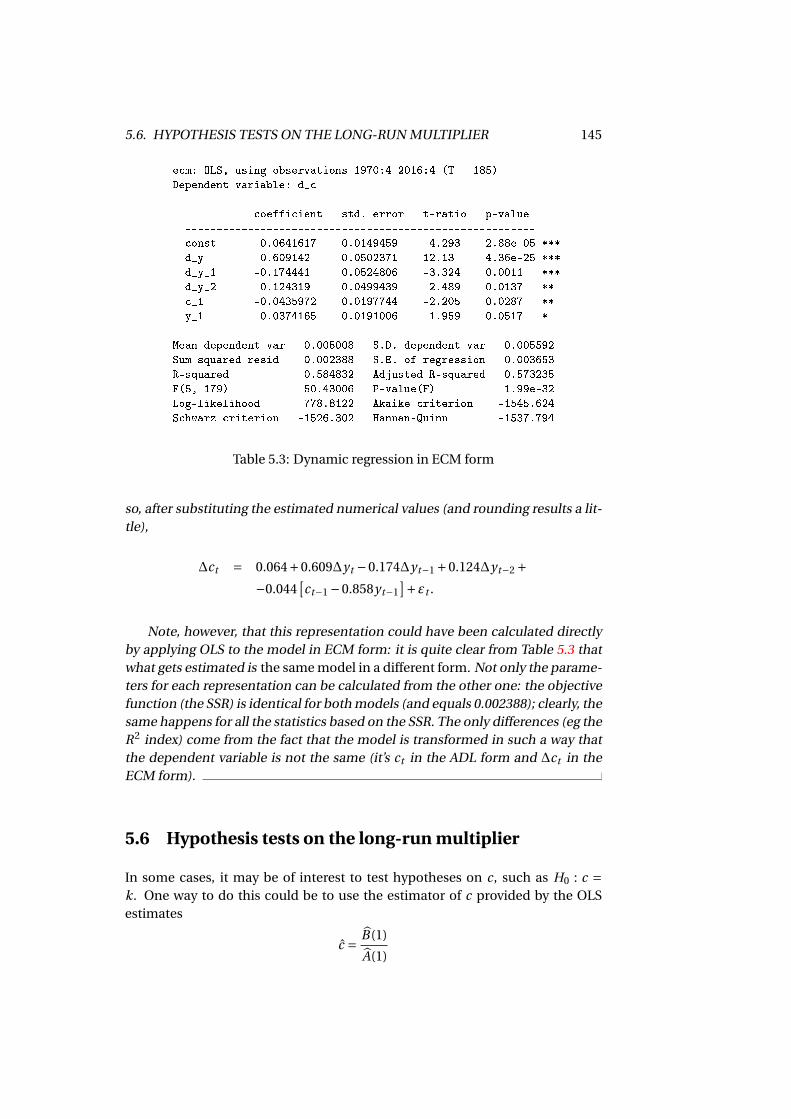
5.6. HYPOTHESIS TESTS ON THE LONG-RUN MULTIPLIER 145
ecm: OLS, using observations 1970:4-2016:4 (T = 185)
Dependent variable: d_c
coefficient std. error t-ratio p-value
--------------------------------------------------------
const 0.0641617 0.0149459 4.293 2.88e-05 ***
d_y 0.609142 0.0502371 12.13 4.36e-25 ***
d_y_1 -0.174441 0.0524806 -3.324 0.0011 ***
d_y_2 0.124319 0.0499439 2.489 0.0137 **
c_1 -0.0435972 0.0197744 -2.205 0.0287 **
y_1 0.0374165 0.0191006 1.959 0.0517 *
Mean dependent var 0.005008 S.D. dependent var 0.005592
Sum squared resid 0.002388 S.E. of regression 0.003653
R-squared 0.584832 Adjusted R-squared 0.573235
F(5, 179) 50.43006 P-value(F) 1.99e-32
Log-likelihood 778.8122 Akaike criterion -1545.624
Schwarz criterion -1526.302 Hannan-Quinn -1537.794
Table 5.3: Dynamic regression in ECM form
so, after substituting the estimated numerical values (and rounding results a lit-tle),
∆ct = 0.064+0.609∆yt −0.174∆yt−1 +0.124∆yt−2 +−0.044
[ct−1 −0.858yt−1
]+εt .
Note, however, that this representation could have been calculated directlyby applying OLS to the model in ECM form: it is quite clear from Table 5.3 thatwhat gets estimated is the same model in a different form. Not only the parame-ters for each representation can be calculated from the other one: the objectivefunction (the SSR) is identical for both models (and equals 0.002388); clearly, thesame happens for all the statistics based on the SSR. The only differences (eg theR2 index) come from the fact that the model is transformed in such a way thatthe dependent variable is not the same (it’s ct in the ADL form and ∆ct in theECM form).
5.6 Hypothesis tests on the long-run multiplier
In some cases, it may be of interest to test hypotheses on c, such as H0 : c =k. One way to do this could be to use the estimator of c provided by the OLSestimates
c = B(1)
A(1)
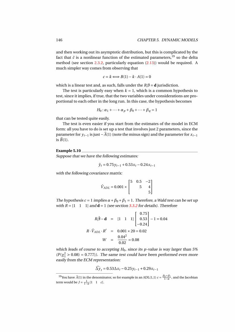
146 CHAPTER 5. DYNAMIC MODELS
and then working out its asymptotic distribution, but this is complicated by thefact that c is a nonlinear function of the estimated parameters,19 so the deltamethod (see section 2.3.2, particularly equation (2.13)) would be required. Amuch simpler way comes from observing that
c = k ⇐⇒ B(1)−k · A(1) = 0
which is a linear test and, as such, falls under the Rβ = d jurisdiction.The test is particularly easy when k = 1, which is a common hypothesis to
test, since it implies, if true, that the two variables under considerations are pro-portional to each other in the long run. In this case, the hypothesis becomes
H0 :α1 +·· ·+αp +β0 +·· ·+βq = 1
that can be tested quite easily.The test is even easier if you start from the estimates of the model in ECM
form: all you have to do is set up a test that involves just 2 parameters, since theparameter for yt−1 is just −A(1) (note the minus sign) and the parameter for xt−1
is B(1).
Example 5.10Suppose that we have the following estimates:
yt = 0.75yt−1 +0.53xt −0.24xt−1
with the following covariance matrix:
VADL = 0.001×5 0.5 −2
5 45
The hypothesis c = 1 implies α+β0+β1 = 1. Therefore, a Wald test can be set upwith R = [1 1 1] and d = 1 (see section 3.3.2 for details). Therefore
Rβ−d = [1 1 1]
0.750.53
−0.24
−1 = 0.04
R · VADL ·R ′ = 0.001×20 = 0.02
W = 0.042
0.02= 0.08
which leads of course to accepting H0, since its p-value is way larger than 5%(P (χ2
1 > 0.08) = 0.777)). The same test could have been performed even moreeasily from the ECM representation:
∆y t = 0.53∆xt −0.25yt−1 +0.29xt−1
19You have A(1) in the denominator, so for example in an ADL(1,1) c = β0+β11−α , and the Jacobian
term would be J = 11−α [1 1 c].
5.7. FORECASTING AND GRANGER CAUSALITY 147
with the associated covariance matrix
VEC M = 0.001×5 0.5 9
5 −1.518
In this case the hypothesis can be written as H0 : B(1)− A(1) = 0, so for the ECMform
Rβ−d = [0 1 1]
0.53−0.25
0.29
= 0.04
R · VEC M ·R ′ = 0.001×20 = 0.02
and of course the W statistic is the same as above.
5.7 Forecasting and Granger causality
One of the cool things you can do with an ADL model is forecasting. Here’s howit works: suppose we have data that goes from t = 1 to t = T , and that our modelof choice is an ADL(1,1). What we can say, on these premises, about yT+1, thatwe haven’t yet observed? The random variable yT+1 can be represented as
yT+1 =αyT +β0xT+1 +β1xT +εT+1; (5.13)
of all the objects that appear on the right-hand side of the equation, the onlyones that are known with certainty at time T are yT and xT . Suppose we alsoknow for certain what the future value xT+1 will be, and call it xT+1 = xT+1.Therefore, since εt is a martingale difference sequence, its conditional expec-tation with respect to ℑT+1 is 0,20 so
E[
yT+1|ℑT] = αyT +β0xT+1 +β1xT
V[
yT+1|ℑT] = σ2
Following the same logic as in Section 3.7, we can use the conditional expecta-tion as predictor and the estimated values for the parameters instead of the trueones. Therefore, our prediction will be
yT+1 = αyT + β0xT+1 + β1xT
and a 95% confidence interval can be constructed as
yT+1 ±1.96× σ20We’re sticking to the definition of ℑT+1 I introduced in Section 5, so ℑT+1 includes xT+1 but
not yT+1; later in this section, we’ll use a different convention.
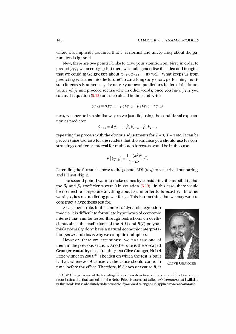
148 CHAPTER 5. DYNAMIC MODELS
where it is implicitly assumed that εt is normal and uncertainty about the pa-rameters is ignored.
Now, there are two points I’d like to draw your attention on. First: in order topredict yT+1 we need xT+1; but then, we could generalise this idea and imaginethat we could make guesses about xT+2, xT+3, . . . as well. What keeps us frompredicting yt farther into the future? To cut a long story short, performing multi-step forecasts is rather easy if you use your own predictions in lieu of the futurevalues of yt and proceed recursively. In other words, once you have yT+1 youcan push equation (5.13) one step ahead in time and write
yT+2 =αyT+1 +β0xT+2 +β1xT+1 +εT+2;
next, we operate in a similar way as we just did, using the conditional expecta-tion as predictor
yT+2 = αyT+1 + β0xT+2 + β1xT+1,
repeating the process with the obvious adjustments for T +3, T +4 etc. It can beproven (nice exercise for the reader) that the variance you should use for con-structing confidence interval for multi-step forecasts would be in this case
V[
yT+k]= 1− (α2)k
1−α2 σ2.
Extending the formulae above to the general ADL(p, q) case is trivial but boring,and I’ll just skip it.
The second point I want to make comes by considering the possibility thatthe β0 and β1 coefficients were 0 in equation (5.13). In this case, there wouldbe no need to conjecture anything about xt , in order to forecast yt . In otherwords, xt has no predicting power for yt . This is something that we may want toconstruct a hypothesis test for.
CLIVE GRANGER
As a general rule, in the context of dynamic regressionmodels, it is difficult to formulate hypotheses of economicinterest that can be tested through restrictions on coeffi-cients, since the coefficients of the A(L) and B(L) polyno-mials normally don’t have a natural economic interpreta-tion per se, and this is why we compute multipliers.
However, there are exceptions: we just saw one ofthem in the previous section. Another one is the so-calledGranger-causality test, after the great Clive Granger, NobelPrize winner in 2003.21 The idea on which the test is builtis that, whenever A causes B , the cause should come, intime, before the effect. Therefore, if A does not cause B , it
21C. W. Granger is one of the founding fathers of modern time series econometrics; his most fa-mous brainchild, that earned him the Nobel Prize, is a concept called cointegration, that I will skipin this book, but is absolutely indispensable if you want to engage in applied macroeconomics.
5.7. FORECASTING AND GRANGER CAUSALITY 149
should have no effect on the quantity we normally use for prediction, i. e. theconditional expectation.
The only difference with the ADL models we’ve considered so far is that,since we’re dealing with predictions about the future, we will want to base ourinference on an information set that collects everything that is known at timet −1, namely
ℑ∗t−1 =
yt−1, yt−2, . . . ,xt−1,xt−2, . . .
;
note that, contrary to the concept of information set ℑt we used so far (definedin section 5.1), ℑ∗
t does not include xt+1; in practice, it collects all informationon yt and xt that is available up to time t . Forecasting, therefore, amounts tofinding
yT+1|T = E[
yT+1|ℑ∗T
].
The subscript “T +1|T ” is customarily read as “at time T +1, based on the infor-mation available at time T ”.
As a consequence, our ADL model
A(L)yt = B(L)xt +εt
will not include xt , but only its lags:
yt =α1 yt−1 +α2 yt−2 +·· ·+β′1xt−1 +β′
2xt−2 +·· ·+ε∗twhere ε∗t is defined as yt −E
[yT+1|ℑ∗
T
]. Clearly, this can also be written as an
ordinary ADL model in which B(0) = 0. The idea that xt does not cause yt isequivalent to the idea B(L) = 0; since a polynomial is 0 if and only if all its coef-ficients are, it is easy to formulate the hypothesis of no-Granger-causality as
H0 :β1 =β2 = . . . =βq = 0
which is of course a system of linear restrictions, that we can handle just fine viathe Rβ = d machine we described in Section 3.3.2.
In the late 1960s, when this idea was introduced, it was hailed as a break-through in economic theory, because for a while this seemed to provide a data-based way to ascertain causal links. For example, a hotly debated point amongmacroeconomists in the 1970 and 80s was: is there a causality direction betweenthe quantity of money and GDP in an economy? If there is, the repercussions oneconomic policy (notably, on the effectiveness of monetary policy) are huge. Inthose days, the concept of Granger-causality seemed to provide a convincinganswer.22
Example 5.11In a humorous article, Thurman and Fisher (1988) collected data on the produc-tion of chickens and eggs from 1930 to 2004, that are depicted in Figure 5.2.
22Readers who are into the history of economics and econometrics might want to take a look atSims (1972).
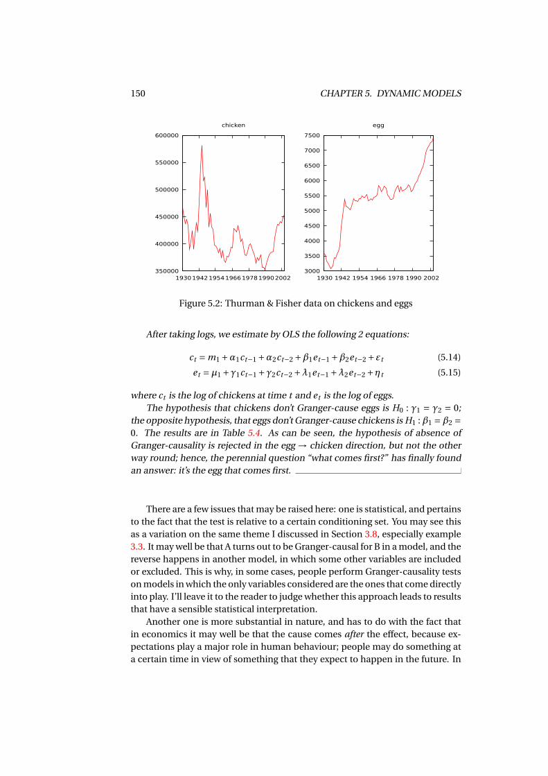
150 CHAPTER 5. DYNAMIC MODELS
350000
400000
450000
500000
550000
600000
1930 1942 1954 1966 1978 1990 2002
chicken
3000
3500
4000
4500
5000
5500
6000
6500
7000
7500
1930 1942 1954 1966 1978 1990 2002
egg
Figure 5.2: Thurman & Fisher data on chickens and eggs
After taking logs, we estimate by OLS the following 2 equations:
ct = m1 +α1ct−1 +α2ct−2 +β1et−1 +β2et−2 +εt (5.14)
et =µ1 +γ1ct−1 +γ2ct−2 +λ1et−1 +λ2et−2 +ηt (5.15)
where ct is the log of chickens at time t and et is the log of eggs.The hypothesis that chickens don’t Granger-cause eggs is H0 : γ1 = γ2 = 0;
the opposite hypothesis, that eggs don’t Granger-cause chickens is H1 :β1 =β2 =0. The results are in Table 5.4. As can be seen, the hypothesis of absence ofGranger-causality is rejected in the egg → chicken direction, but not the otherway round; hence, the perennial question “what comes first?” has finally foundan answer: it’s the egg that comes first.
There are a few issues that may be raised here: one is statistical, and pertainsto the fact that the test is relative to a certain conditioning set. You may see thisas a variation on the same theme I discussed in Section 3.8, especially example3.3. It may well be that A turns out to be Granger-causal for B in a model, and thereverse happens in another model, in which some other variables are includedor excluded. This is why, in some cases, people perform Granger-causality testson models in which the only variables considered are the ones that come directlyinto play. I’ll leave it to the reader to judge whether this approach leads to resultsthat have a sensible statistical interpretation.
Another one is more substantial in nature, and has to do with the fact thatin economics it may well be that the cause comes after the effect, because ex-pectations play a major role in human behaviour; people may do something ata certain time in view of something that they expect to happen in the future. In
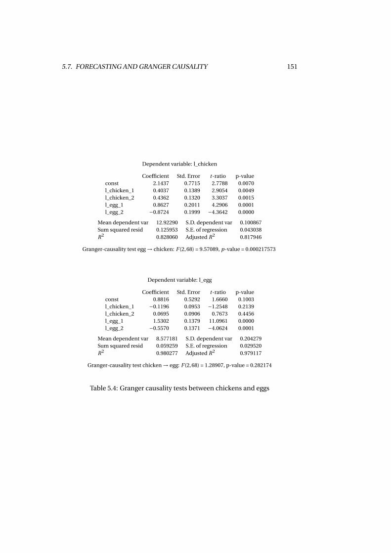
5.7. FORECASTING AND GRANGER CAUSALITY 151
Dependent variable: l_chicken
Coefficient Std. Error t-ratio p-valueconst 2.1437 0.7715 2.7788 0.0070l_chicken_1 0.4037 0.1389 2.9054 0.0049l_chicken_2 0.4362 0.1320 3.3037 0.0015l_egg_1 0.8627 0.2011 4.2906 0.0001l_egg_2 −0.8724 0.1999 −4.3642 0.0000
Mean dependent var 12.92290 S.D. dependent var 0.100867Sum squared resid 0.125953 S.E. of regression 0.043038R2 0.828060 Adjusted R2 0.817946
Granger-causality test egg → chicken: F (2,68) = 9.57089, p-value = 0.000217573
Dependent variable: l_egg
Coefficient Std. Error t-ratio p-valueconst 0.8816 0.5292 1.6660 0.1003l_chicken_1 −0.1196 0.0953 −1.2548 0.2139l_chicken_2 0.0695 0.0906 0.7673 0.4456l_egg_1 1.5302 0.1379 11.0961 0.0000l_egg_2 −0.5570 0.1371 −4.0624 0.0001
Mean dependent var 8.577181 S.D. dependent var 0.204279Sum squared resid 0.059259 S.E. of regression 0.029520R2 0.980277 Adjusted R2 0.979117
Granger-causality test chicken → egg: F (2,68) = 1.28907, p-value = 0.282174
Table 5.4: Granger causality tests between chickens and eggs
152 CHAPTER 5. DYNAMIC MODELS
fact, standard economic theory assumes that agents are rational and forward-looking: they base all their choices on the expectations they have about the fu-ture.
There are many examples I could give you, but I’ll simply hint at a widelyused one: people normally do their Christmas shopping before Christmas, soit would be legitimate to say that gift purchases Granger-cause Christmas. Theproblem here is that in this case the statistical concept of Granger causality doesnot agree very much with the notion of causality we use in everyday life (and isarguably what we care about in economics).
5.A Assorted results
5.A.1 Inverting polynomials
Let us begin by noting that, for any a 6= 1,
n∑i=0
ai = 1−an+1
1−a, (5.16)
which is easy to prove: call
S =n∑
i=0ai = 1+a +a2 +·· ·+an ; (5.17)
of coursea ·S = a +a2 +·· ·+an+1 (5.18)
and therefore, by subtracting (5.18) from (5.17), S(1− a) = 1− an+1, and henceequation (5.16).
If a is a small number (|a| < 1), then an → 0, and therefore∑∞
i=0 ai = 11−a . By
setting a = αL, you may say that, for |α| < 1, the inverse of (1−αL) is (1+αL +α2L2 +·· · ), that is
(1−αL)(1+αL+α2L2 +·· · ) = 1,
or, alternatively,1
1−αL=
∞∑i=0
αi Li
provided that |α| < 1. Now consider a n-th degree polynomial P (x):
P (x) =n∑
j=0p j x j
If P (0) = p0 = 1, then P (x) can be written as the product of n first-degree poly-nomials as follows:23
P (x) =n∏
j=1
(1− 1
λ jx
)(5.19)
23If you don’t believe me, google for “Fundamental theorem of algebra”.
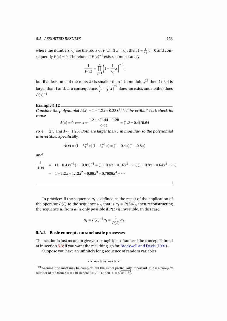
5.A. ASSORTED RESULTS 153
where the numbers λ j are the roots of P (x): if x = λ j , then 1− 1λ j
x = 0 and con-
sequently P (x) = 0. Therefore, if P (x)−1 exists, it must satisfy
1
P (x)=
n∏j=1
(1− 1
λ jx
)−1
;
but if at least one of the roots λ j is smaller than 1 in modulus,24 then 1/|λ j | is
larger than 1 and, as a consequence,(1− 1
λ jx)−1
does not exist, and neither does
P (x)−1.
Example 5.12Consider the polynomial A(x) = 1−1.2x +0.32x2; is it invertible? Let’s check itsroots:
A(x) = 0 ⇐⇒ x = 1.2±p1.44−1.28
0.64= (1.2±0.4)/0.64
so λ1 = 2.5 and λ2 = 1.25. Both are larger than 1 in modulus, so the polynomialis invertible. Specifically,
A(x) = (1−λ−11 x)(1−λ−1
2 x) = (1−0.4x)(1−0.8x)
and
1
A(x)= (1−0.4x)−1(1−0.8x)−1 = (1+0.4x +0.16x2 +·· · )(1+0.8x +0.64x2 +·· · )= 1+1.2x +1.12x2 +0.96x3 +0.7936x4 +·· ·
In practice: if the sequence at is defined as the result of the application ofthe operator P (L) to the sequence ut , that is at = P (L)ut , then reconstructingthe sequence ut from at is only possible if P (L) is invertible. In this case,
ut = P (L)−1at = 1
P (L)at .
5.A.2 Basic concepts on stochastic processes
This section is just meant to give you a rough idea of some of the concept I hintedat in section 5.3; if you want the real thing, go for Brockwell and Davis (1991).
Suppose you have an infinitely long sequence of random variables
. . . , xt−1, xt , xt+1, . . .
24Warning: the roots may be complex, but this is not particularly important. If z is a complex
number of the form z = a +bi (where i =p−1), then |z| =√
a2 +b2.
154 CHAPTER 5. DYNAMIC MODELS
where the index t is normally taken to mean “time” (although in fact it needn’tbe). This sequence is a stochastic process.25 When we observe a time series, weobserve a part of the realisation of a stochastic process (also called a trajectoryof the process).
If we take two different elements of the sequence, say xs and xt (with s 6= t ),we could wonder what their joint distribution is. The two fundamental proper-ties of the joint distribution that we are interested in are:
1. is the joint distribution stable through time? That is, is the joint distribu-tion of (xs , xt ) the same as (xs+1, xt+1) ?
2. Is it likely that xs and xt become independent (or nearly so) if |t − s| islarge?
Property number 1 refers to the idea that the point in time when we ob-serve the process should be irrelevant: the probability distribution of the datawe see today (xs , xt ) should be the same as the one for an observer in the past(xs−100, xt−100) or in the future (xs+100, xt+100). This gives rise to the concept ofstationarity. A stochastic process is said to be weakly stationary, or covariancestationary, or second-order stationary if the covariance between xs and xt (alsoknown as autocovariance) exists and is independent of time. In formulae:
γh = Cov[xt , xt+h]
note that γh , the autocovariance of order h, is a function of h only, not of t ; ofcourse, γ0 is just V[xt ]. If this is the case, the internal structure of correlationbetween points in time is often described via the autocorrelation sequence (orautocorrelation function, often abbreviated as ACF), defined as
ρh = γh
γ0.
Property number 2, instead, is what we realistically imagine should happenwhen we observe many phenomena through time: if s and t are very far apart,what happened at time s one should contain little or no information on whathappened at time t . For example: the number of children born in the Kingdomof Verduria 400 years ago should contain no useful information on the numberof children born in the Kingdom of Verduria today. This intuition can be trans-lated into maths in a number of different ways. A common one is ergodicity.While a formal definition of ergodicity would require a hefty investment in mea-sure theory, if a process is covariance stationary, ergodicity amounts to absolutesummability of its autocovariances. The property
∞∑i=0
|γi | = M <∞
25It’s not inappropriate to think of stochastic processes as infinite-dimensional randomvariables. Using the same terminology as in section 2.2.1, we may think of the sequence. . . , xt−1(ω), xt (ω), xt+1(ω), . . . as the infinite-dimensional outcome of one point in the state spaceω ∈Ω.
5.A. ASSORTED RESULTS 155
ensures that limh→∞ |γh | = 0 (so correlation between distant events should benegligible), but most importantly, that the sample mean of an observed stochas-tic process is a consistent estimator of the true mean of the process:
1
T
T∑t=1
xtp−→ E[xt ] .
Note that the above expression can be considered as one of the many versionsof the Law of Large Numbers.
A large part of the statistical analysis of time series is based on the idea thatthe time series we observe are realisations of stationary and ergodic processes(or can be transformed to this effect).
5.A.3 Why martingale difference sequences are serially uncorrelated
Here’s a rapid proof: if εt is a MDS with respect to ℑt , then
E[εt |ℑt ] = E[εt |xt ,xt−1, . . . , yt−1, yt−2, . . .
]= 0.
Now, observe that εt−1 is defined as εt−1 = yt−1 −E[
yt−1|ℑt−1]; since both ele-
ments of the right-hand side of the equation are contained in ℑt , then εt−1 ∈ℑt ;moreover, ℑt ⊇ℑt−1 ⊇ℑt−2 . . ., so clearly all lags of εt are all contained in ℑt (seefootnote 6 in this chapter). As a consequence, we can use the law of iteratedexpectations (2.7) as follows:
Cov[εt ,εt−k ] = E[εt ·εt−k ] = E[E[εt ·εt−k ] |ℑt ] == E[E[εt |ℑt ] ·εt−k ] = E[0 ·εt−k ] == 0
A second argument, perhaps more intuitive, rests directly on the definitionof a MDS: if εt is a MDS with respect to ℑt , then its expectation conditional onℑt−k (for k > 0) must also be 0, because ℑt−k is a subset of ℑt . But that meansthat the expectation of any future element εt+k conditional on the present infor-mation set ℑt is 0. In formulae:
E[εt |ℑt ] = 0ℑt−k ⊆ℑt for k > 0
=⇒ E[εt |ℑt−k ] = E[εt+k |ℑt ] = 0
This is tantamount to saying that εt is effectively unpredictable. But then, ifCov[εt ,εt−k ] 6= 0, εt wouldn’t be totally unpredictable, because there would besome information in the past about the future. Therefore, the autocorrelationsof a MDS must be 0 for any k.
156 CHAPTER 5. DYNAMIC MODELS
5.A.4 From ADL to ECM
Let’s begin with a preliminary result (which I’m not going to prove):
If P (x) is a polynomial whose degree is n > 0 and a is a scalar, you can always finda polynomial Q(x), whose degree is (n −1), such that
P (x) = P (a)+Q(x)(a −x);
if n = 0, obviously Q(x) = 0.
For example, the reader is invited to check that, if we choose a = 1, the poly-nomial P (x) = 1−1.8x +0.4x2 can be written as
P (x) =−0.4+ (1−0.8x)(1−x)
where P (1) =−0.4 and Q(x) = 1−0.8x.Now consider P (L), a polynomial in the lag operator of degree n ≥ 1, and
apply the result above twice in a row, once with a = 0 and then with a = 1:
P (L) = P (0)−Q(L) ·L (5.20)
Q(L) = Q(1)+P∗(L)(1−L) (5.21)
If n = 1, evidently P∗(L) = 0. Otherwise, the order of Q(L) is (n − 1) and theorder of P∗(L) is (n−2). If you evaluate equation (5.20) in L = 1, you have P (1) =P (0)−Q(1), so that equation (5.21) becomes
Q(L) = P (0)−P (1)+P∗(L)(1−L)
and therefore, using equation (5.20) again,
P (L) = P (0)− [P (0)−P (1)+P∗(L)(1−L)
] ·L = P (0)∆+P (1)L−P∗(L)∆ ·L.
The actual form of the P∗(L) polynomial is not important: all we need is know-ing that it exists, so that the decomposition of P (L) we just performed is alwayspossible. As a consequence, every sequence P (L)zt can be written as:
P (L)zt = P (0)∆zt +P (1)zt−1 −P∗(L)∆zt−1.
Now apply this result to both sides of the ADL model A(L)yt = B(L)xt +εt :
∆yt + A(1)yt−1 − A∗(L)∆yt−1 = B(0)∆xt +B∗(L)∆xt−1 +B(1)xt−1 +εt ;
(note that A(0) = 1 by construction). After rearranging terms, you obtain theECM representation proper:
∆yt = B(0)∆xt + A∗(L)∆yt−1 +B∗(L)∆xt−1 − A(1)[
yt−1 −c′xt−1]+εt
where c′ = B(1)A(1) contains the long-run multipliers. In other words, the variation
of yt over time is expressed as the sum of three components:

5.A. ASSORTED RESULTS 157
1. the external unpredictable shock εt ;
2. a short-run transitory component: B(0)∆xt+A∗(L)∆yt−1+B∗(L)∆xt−1; thefirst coefficient, B(0), gives you the instantaneous effect of xt on yt ;
3. a long-run component whose base ingredient is the long-run multiplier c.

158 CHAPTER 5. DYNAMIC MODELS
Chapter 6
Instrumental Variables
The arguments I presented in chapter 3 should have convinced the reader thatOLS is an excellent solution to the problem of estimating linear models of thekind
y = Xβ+ε,
where ε is defined as y−E[y|X]
, with the appropriate adjustments for dynamicmodels; the derived property E[ε|X] = 0 is the key ingredient for guaranteeingconsistency of OLS as an estimator of β. With some extra effort, we can alsoderive asymptotic normality and have all the hypothesis testing apparatus atour disposal.
In some cases, however, this is not what we need. What we have implicitlyassumed so far is that the parameters of economic interest are the same as thestatistical parameters that describe the conditional expectation (or functionsthereof, like for example marginal effects or multipliers in dynamic models).
Sometimes, this might not be the case. As anticipated in section 3.5, thishappens when the model we have in mind contains explanatory variables that,in common economics parlance, are said to be endogenous. In the next section,I will give you a few examples where the quantities of interpretative interest arenot computable from the regression parameters. Hence, it should come as nosurprise that OLS is not a usable tool for this purpose: this is why we’ll want touse a different estimator, known as instrumental variables estimator, or IV forshort.
6.1 Examples
6.1.1 Measurement error
Measurement error is what you get when one or more of your explanatory vari-able are measured imperfectly. Suppose you have the simplest version of a linearmodel, where everything is a scalar:
yi = x∗i β+εi (6.1)
159
160 CHAPTER 6. INSTRUMENTAL VARIABLES
where E[
yi |x∗i
]= x∗i β and β is our parameter of interest. The problem is that we
do not observe x∗i directly; instead, all we have is a version of x∗
i that is contam-inated by some measurement error:
xi = x∗i +ηi (6.2)
where ηi is a zero-mean random variable, independent of x∗i and εi , with vari-
ance σ2η > 0; clearly, the larger σ2
η > 0 is, the worse is the quality of our measure-ment for the variable of interest x∗
i . One may think that, since ηi is, so to speak,“neutral”, setting up a model using xi instead of x∗
i would do no harm. Instead,this is not the case: unfortunately, OLS regression yi on xi won’t give you a con-sistent estimator of β. This is quite easy to prove: combine the two equationsabove to get
yi = xiβ+ (εi −βηi
)= xiβ+ui (6.3)
so
β=∑n
i=1 xi yi∑ni=1 x2
i
=∑n
i=1 xi (xiβ+ui )∑ni=1 x2
i
=β+∑n
i=1 xi ui∑ni=1 x2
i
From the assumptions above, you get
E[xi ui ] = E[(x∗
i +ηi )(εi −βηi )]= E
[x∗
i εi]−βE
[x∗
i ηi]+E
[ηiεi
]−βE[η2
i
]== −βσ2
η
If we define Q = E[x2
i
], clearly
βp−→β−
βσ2η
Q=β
(1−
σ2η
Q
)6=β
It can be proven that 0 < σ2η < Q,1 so two main conclusions can be drawn from
the equation above: first, the degree of inconsistency of OLS is proportional tothe size of measurement error σ2
η relative to Q; second, the asymptotic bias is
such that 0 < |plim(β) | < |β|; that is, the estimated effect is smaller than the true
one. This is often called attenuation.
As the rest of this chapter should hopefully make clear, the reason why OLSdoesn’t work as we’d like it to work lies in the fact that equation (6.3) does notsplit yi into a conditional expectation and a disturbance term. It can be shownthat the regression function E
[yi |xi
]is not equal to xiβ: if it were, E[xi ui ] would
be zero, but we just showed it isn’t. Since OLS is programmed to estimated theparameters of a conditional expectation, you can’t expect it to come up withanything else.
1Come on, it’s easy, do it by yourself.
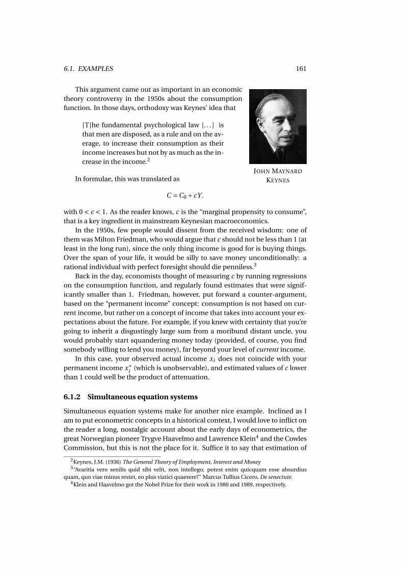
6.1. EXAMPLES 161
JOHN MAYNARD
KEYNES
This argument came out as important in an economictheory controversy in the 1950s about the consumptionfunction. In those days, orthodoxy was Keynes’ idea that
[T]he fundamental psychological law [. . . ] isthat men are disposed, as a rule and on the av-erage, to increase their consumption as theirincome increases but not by as much as the in-crease in the income.2
In formulae, this was translated as
C =C0 + cY .
with 0 < c < 1. As the reader knows, c is the “marginal propensity to consume”,that is a key ingredient in mainstream Keynesian macroeconomics.
In the 1950s, few people would dissent from the received wisdom: one ofthem was Milton Friedman, who would argue that c should not be less than 1 (atleast in the long run), since the only thing income is good for is buying things.Over the span of your life, it would be silly to save money unconditionally: arational individual with perfect foresight should die penniless.3
Back in the day, economists thought of measuring c by running regressionson the consumption function, and regularly found estimates that were signif-icantly smaller than 1. Friedman, however, put forward a counter-argument,based on the “permanent income” concept: consumption is not based on cur-rent income, but rather on a concept of income that takes into account your ex-pectations about the future. For example, if you knew with certainty that you’regoing to inherit a disgustingly large sum from a moribund distant uncle, youwould probably start squandering money today (provided, of course, you findsomebody willing to lend you money), far beyond your level of current income.
In this case, your observed actual income xi does not coincide with yourpermanent income x∗
i (which is unobservable), and estimated values of c lowerthan 1 could well be the product of attenuation.
6.1.2 Simultaneous equation systems
Simultaneous equation systems make for another nice example. Inclined as Iam to put econometric concepts in a historical context, I would love to inflict onthe reader a long, nostalgic account about the early days of econometrics, thegreat Norwegian pioneer Trygve Haavelmo and Lawrence Klein4 and the CowlesCommission, but this is not the place for it. Suffice it to say that estimation of
2Keynes, J.M. (1936) The General Theory of Employment, Interest and Money3“Avaritia vero senilis quid sibi velit, non intellego; potest enim quicquam esse absurdius
quam, quo viae minus restet, eo plus viatici quaerere?” Marcus Tullius Cicero, De senectute.4Klein and Haavelmo got the Nobel Prize for their work in 1980 and 1989, respectively.
162 CHAPTER 6. INSTRUMENTAL VARIABLES
systems of equation is the first autonomous contribution of econometrics to thegeneral arsenal of statistical tools.
TRYGVE
HAAVELMO
The reason why the estimation of parameters in simul-taneous systems may be tricky is relatively easy to see byfocusing on the distinction between parameters of interestand parameters of the conditional mean.
Consider one of the simplest examples of simultane-ous equation system in economics: a two-equation linearmodel of supply and demand for a good.
qt = α0 −α1pt +ut (6.4)
pt = β0 +β1qt + vt , (6.5)
equation (6.4) is the demand equation (quantity at time tas a function of price at time t ), (6.5) is supply (price as a function of quan-tity); the two disturbance terms ut and vt represent random shocks to the twocurves. For example, ut could incorporate random fluctuations in demanddue to shifting customer preferences, fluctuations in disposable income and soforth; vt , instead could be non-zero because of productivity shifts due to ran-dom events (think for example weather for agricultural produce). Assume thatE[ut ] = E[vt ] = 0.
If you considered the two equations separately, one may think of estimat-ing their parameters by using OLS, but this would be a big mistake, since the“systematic part” of each of the two equations is not a conditional expectation.
One simple way to convince yourself is simply to consider that if E[qt |pt
]is
upward (downward) sloping, the correlation between qt and pt must be posi-tive (negative), and therefore there’s no way the reverse conditional expectationE
[pt |qi
]can be downward (upward) sloping. Since the demand function goes
down and the supply function goes up, at least one of them cannot be a condi-tional expectation.
However, a more rigorous proof can be given: take the demand curve (6.4):if the expression (α0 −α1pt ) were in fact the conditional expectation of qt to pt ,then E
[ut |pt
]should be 0. Now substitute (6.4) into equation (6.5):
pt = β0 +β1(α0 −α1pt +ut )+ vt
= (β0 +β1α0)− (β1α1)pt + (vt +β1ut ) ⇒(1+β1α1)pt = (β0 +β1α0)+ (vt +β1ut ) ⇒ (6.6)
pt = π1 +ηt , (6.7)
where the constant π1 is β0+β1α0
1+β1α1and ηt = vt+β1ut
1+β1α1is a zero-mean random vari-
able. The covariance between pt and ut is easy to compute:
Cov[pt ,ut
] = E[pt ·ut
]= E[utπ1 +utηt
]= 0+E[ut · (vt +β1ut )
]== Cov[vt ,ut ]+β1V (ut )
6.2. THE IV ESTIMATOR 163
Now, unless the covariance between vt and ut happens to be exactly equal to−β1V (ut ) (and there is no reason why it should), Cov
[pt ,ut
] 6= 0. Borrowing onthe definition I gave in Section 3.5, the variable pt is clearly endogenous.
But if Cov[pt ,ut
] 6= 0, then E[ut |pt
]can’t be 0 either; therefore, (α0 −α1pt )
can’t be E[qt |pt
], and as a consequence there’s no way that OLS applied to equa-
tion (6.4) (that is, regressing quantity on a constant and price) could be a con-sistent estimator of α0 and α1.
To be more specific: even assuming that E[qt |pt
]is a linear function like
E[qt |pt
]= γ0 +γ1pt ,
OLS gives you an excellent estimate of the coefficients γ0 and γ1; unfortunately,they are not the same thing as α0 and α1.
Of course, the same argument in reverse could be applied to the supplyequation so regressing pt on qt won’t give you good estimates of β0 and β1, ei-ther. This example will be generalised in section 6.6.2.
6.2 The IV estimator
In a standard linear model yi = x′iβ+εi . As we argued in chapter 3, the assump-tion x′β = E
[y |x]
is crucial for the consistency of the OLS statistic as an estimatorof β; in fact, you could see this assumption as a definition of β, in that β is theonly vector for which the following equation is true:
E[X′(y−X′β)
]= 0. (6.8)
The OLS statistic β, instead, is implicitly defined by the relationship
X′(y−Xβ) = 0. (6.9)
which corresponds to the first-order conditions for the minimisation of the sumof squared residuals (see section 1.3.2, especially equation (1.10)); note that equa-tion (6.9) can be seen as the sample equivalent of equations (6.8). The fact thatthe OLS statistic β works quite nicely as an estimator of its counterpart β justagrees with common sense.
If, on the contrary, the parameter of interest β satisfies an equation otherthan (6.8), then we may proceed by analogy and use, as an estimator, a statisticβ that satisfies the corresponding sample property. In this chapter, we assumewe have a certain number of observable variables W for which
E[W′(y−Xβ)
]= 0. (6.10)
The corresponding statistic will then be implicitly defined by
W′(y−Xβ) = 0. (6.11)
164 CHAPTER 6. INSTRUMENTAL VARIABLES
The variables W are known as instrumental variables, or, more concisely, in-struments. The so-called “simple” IV estimator can then be defined as follows:if we had a matrix W, of the same size as X, satisfying (6.10), then then we maydefine a statistic β such that (6.11) holds:
W′(y−Xβ) = 0 =⇒ W′X · β = W′y.
In a parallel fashion, the difference ε = y−Xβ is not defined as the differencebetween y and it conditional mean, but rather as a zero-mean random variablewhich describes how much y deviates from its “standard” value, as described bythe “structural” relationship Xβ. A term that we use in this context is structuraldisturbance, or just “disturbance” when no confusion arises. Given this defini-tion, there is no guarantee that the structural disturbance should be orthogonalto the regressors.
Since W has as many columns as X, then the matrix W′X is square; if it’s alsoinvertible, then β is
β = (W′X)−1W′y; (6.12)
this is sometimes called the “simple” IV estimator.The actual availability of the variables W may be a problem, sometimes. In
fact, collecting observable data that can be used as instrument is a bit of an art,although in many cases the choice of instruments is dictated by economic in-tuition. In Section 6.6, we will look at the examples provided in Section 6.1 andsuggest possible solutions. However, before doing so, it is convenient to con-sider a generalisation.
6.2.1 The generalised IV estimator
What if the number of columns of W (call it m) was different from number ofcolumns from X (call it k)? Of course, the matrix W′X wouldn’t be square andtherefore not invertible. While there’s no remedy for the case m < k, one mayargue that in the opposite case we could just drop m −k columns from W andproceed as above. While this makes sense, the reader will probably feel uneasyat the thought of dumping information deliberately. And besides, how do wechoose which columns to drop from W?
Fortunately, there is a solution: assume, for simplicity, that the covariancematrix of the structural disturbances is a multiple of the identity matrix:5
E[εε′|W]=σ2I.
By hypothesis, E[ε|W] = 0; therefore,
E[W′εε′W|W]=σ2W′W =σ2Ω.
5In fact, this assumption is not strictly necessary, but makes for a cleaner exposition.
6.2. THE IV ESTIMATOR 165
Now define v , C and e as
vm×1
= W′y Cm×k
= W′X em×k
= W′ε;
so the following equality holds:
v =Cβ+e, (6.13)
Equation (6.13) may be seen as a linear model where the disturbance term haszero mean and covariance matrix σ2Ω. The number of explanatory variables isk (the column size of X) but the peculiar feature of this model is that the numberof “observations” is m (the column size of W).
Since Ω is observable (up to a constant), we may apply the GLS estimator(see 4.2.1) to (6.13) and write
β = [C ′Ω−1C
]−1C ′Ω−1v = [
X′W(W′W)−1W′X]−1
X′W(W′W)−1W′y == (X′PWX)−1X′PWy. (6.14)
DENIS SARGAN
This clever idea is due to the English econometricianDenis Sargan,6 whose name will also crop up later, in sec-tion 6.7.1.
The estimator β in the equation above is technicallycalled the Generalised IV Estimator, or GIVE for short.However, proving that (6.12) is just a special case of (6.14)when m = k is a simple exercise in matrix algebra, left tothe reader as an exercise, so when I speak of the IV estima-tor, what I mean is (6.14).
When m = k, the model is said to be exactly identified,as the estimator is based on solving (6.11), which is a sys-tem of m equations in m unknowns; if W′X is invertible, it has one solution.
On the contrary, if m > k, (6.11) becomes a system with more equations thanunknowns, so a solution does not ordinarily exist. The statistic we use is not asolution of (6.11), but is rather defined by re-casting the problem as a sui generisOLS model as in (6.13).
In this case, we say the model is over-identified and the difference (m −k)is referred to as over-identification rank. The opposite case, when m < k, is atextbook case of under-identification, which I described in section 2.5. In short,one may say that a necessary condition for the existence of the IV estimator isthat m ≥ k; this is known as the order condition.
6For historical accuracy, it must be said that the idea of IV estimation was first put forwardas early as 1953 by the Dutch genius Henri Theil. But it was Sargan who created the modernapproach, in an article appeared in 1958.
166 CHAPTER 6. INSTRUMENTAL VARIABLES
As a by-product from estimating β, you also get a residual vector ε= y−Xβ,so that an estimator of σ2 is readily available:
σ2 = ε′εn
.
As shown in section 6.A.1, it can be proven that, under the set of assumptions Ijust made, the statistics β and σ2 are CAN estimators. Therefore, the whole test-ing apparatus we developed in Chapter 3 can be applied without modificationssince p
n(β−β)d−→ N (0,V ) .
The precise form of the asymptotic covariance matrix V is not important here;see 6.A.1. What is important in practice is that, under homoskedasticity, we havean asymptotically valid matrix we can use for hypothesis testing, which is
V = σ2(X′PWX)−1.
In more general cases, robust alternatives (see section 4.2.2) are available.
Just like OLS, the IV estimator may be definedas the solution of an optimisation problem:
β =Argminβ∈Rk
ε(β)′PWε(β)
(compare the above expression with equation(1.14)).In this book, we will not make much use ofthis property. However, defining β in this way
would be the first step towards seeing it as amember of a very general category of estima-tors known as GMM (Generalised Method ofMoments) estimators, which includes practi-cally all estimators used in modern economet-rics. The theory of GMM is beautiful: as astarting point, I heartily recommend Hayashi(2000).
6.2.2 The instruments
I will not distract the reader here with technicalities on the asymptotics of the IVestimator; you’ll find those in Section 6.A.1. Here, I’m going to focus on two nec-essary conditions for consistency of β and explore what requisites they implyfor the variables we choose as instruments. The two conditions are:
1. 1n
∑wiεi
p−→ 0
2. 1n
∑xi w′
ip−→ A, where A is a k ×m matrix with rank k.
Condition 1 is more or less guaranteed by (6.10), that is by wi being exoge-nous, which basically means “uncorrelated with the structural disturbance” εi ;if this requirement isn’t met, the limit in probability of β is not β. End of story.
The implications of condition 2 are more subtle. The first one is: since therank of A cannot be k if m < k, you need to have at least as many instrumentsas regressors. The good news is, this condition is not as stringent as it may seemat first sight: the fact that E[xi ·εi ] is not a vector of zeros does not necessarily
6.2. THE IV ESTIMATOR 167
mean that all its elements are nonzero. Some of the explanatory variables maybe exogenous; in fact, in empirical models the subset of explanatory variablesthat may be suspected of endogeneity is typically rather small. Therefore, theexogenous subset of xi is perfectly adequate to serve as an instrument, obviousexamples being deterministic variables such as the constant. What the ordercondition really means is that, for each endogenous explanatory variable, weneed at least one instrument not also used as a regressor.
Clearly, m ≥ k is not a sufficient condition for A to have rank k. For exam-ple, A may be square but have a column full of zeros. This would happen, forexample, if the corresponding instrument was independent of all regressors x.The generalisation of this idea leads to the concept of relevance.7 The instru-ments must not only be exogenous, but must also be related to the explanatoryvariables.8
Note a fundamental difference between the order condition and the rele-vance condition: the order condition can be checked quite easily (all you haveto do is count the variables); and even if you can’t be bothered with checking, ifthe order condition fails the IV estimator β is not computable, since (X′PWX) issingular and your software will complain about this.
The relevance condition, instead, is much trickier to spot, since (with prob-ability 1) 1
n
∑xi w′
i will have rank k even if A doesn’t. Hence, if rk(A) < k, you willbe able to compute β, but unfortunately it will be completely useless as an esti-mator. It can be proven that, in such an unfortunate case, the limit in probabilityof β is not a constant, but rather a random variable, so there’s no way it can be aconsistent estimator for any parameter.
In order to make this point clearer, let me give you an example. Supposethat the three random variables yi , xi and wi were continuous and scalar andimagine that that wi is not relevant. The IV estimator would simply be
β = n−1 ∑ni=1 xi yi
n−1 ∑ni=1 wi xi
;
now focus on the denominator of the expression above: clearly, the probabilitythat n−1 ∑n
i=1 wi xi = 0 is 0, so the probability that β exists is 1 for any finite n.However, if you compute its probability limit, you see the problem very quickly:
if wi is not relevant, then n−1 ∑ni=1 wi xi
p−→ A = 0 (which has, of course, rank 0instead of 1, as we would require). Therefore the denominator will be a nonzeronumber which becomes smaller and smaller as n →∞. The reader should easilysee that in this case we can’t expect the asymptotic distribution of β to collapseto a point. In this case the estimator is not inconsistent because it converges tothe wrong value, but rather because it doesn’t converge at all.
7In other contexts, what I call the relevance condition is known as the rank condition.8It should be noted that these properties are, to some extent, contradictory: if X and ε are
correlated, any variable perfectly correlated to X could not be orthogonal to ε. The trick here isthat W is not perfectly correlated to X.
168 CHAPTER 6. INSTRUMENTAL VARIABLES
Finally, instruments should be as “strong” as possible. The precise mean-ing of this phrase is the object of Section 6.7.2: here, I’ll just mention the factthat inference with IV models could be quite problematic in finite samples, sincethe asymptotic approximations that we ordinarily use may work quite poorly. Acommon source of problems is the case of weak instruments: variables that arerelevant, but whose connection with the regressors is so feeble that you need aninordinately large data set to use them for your purposes. This point will (hope-fully) become clearer later, in the context of “two-stage” estimation (Section 6.5).
6.3 An example with real data
For this example, we are going to use a great classic from applied labour eco-nomics: the “Mincer wage equation”; the idea is roughly to have a model likethe following:
yi = z′iβ0 +eiβ1 +εi (6.15)
where yi is the log wage for an individual, ei is their education level and thevector zi contains other characteristics we want to control for (gender, work ex-perience, etc). The parameter of interest is β1, which measures the returns toeducation and that we would expect to be positive.
The reader, at this point, may dimly recall that we already estimated an equa-tion like this, in section 1.6. Back then, we did not have the tools yet for interpret-ing the results from an inferential perspective, but the results were in agreementwith commons sense. Why would we want to go back to a wage equation here?
The literature has long recognised that education may be endogenous, be-cause the amount of education individuals receive is (ordinarily) decided by theindividuals themselves. In practice, if the only reason to get an education is tohave access to more lucrative jobs, individuals solve an optimisation problemwhere they decide, among other things, their own education level. This givesrise to a an endogeneity problem.9
For the reader’s convenience, I’ll reproduce here OLS estimates in Table 6.1.If education is endogenous, as economic theory suggests may be, then the “re-turns to education” parameter we find in the OLS output (about 5.3%) is a validestimate of the marginal effect of education on the conditional expectation ofwage, but is not a valid measure of the causal effect of education on wages, thatis the increment in wage that an individual would have had if they had receivedan extra year of education.
I will now estimate the same equation via IV: the instruments I chose forthis purpose are (apart from the three regressors other than education, whichI take as exogenous) two variables that I will assume, for the moment, as validinstruments:
9The literature on this topic is truly massive. A good starting point is Card (1999).
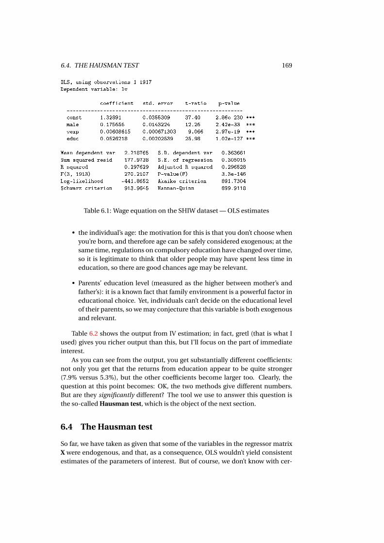
6.4. THE HAUSMAN TEST 169
OLS, using observations 1-1917
Dependent variable: lw
coefficient std. error t-ratio p-value
----------------------------------------------------------
const 1.32891 0.0355309 37.40 2.86e-230 ***
male 0.175656 0.0143224 12.26 2.42e-33 ***
wexp 0.00608615 0.000671303 9.066 2.97e-19 ***
educ 0.0526218 0.00202539 25.98 1.02e-127 ***
Mean dependent var 2.218765 S.D. dependent var 0.363661
Sum squared resid 177.9738 S.E. of regression 0.305015
R-squared 0.297629 Adjusted R-squared 0.296528
F(3, 1913) 270.2107 P-value(F) 3.3e-146
Log-likelihood -441.8652 Akaike criterion 891.7304
Schwarz criterion 913.9645 Hannan-Quinn 899.9118
Table 6.1: Wage equation on the SHIW dataset — OLS estimates
• the individual’s age: the motivation for this is that you don’t choose whenyou’re born, and therefore age can be safely considered exogenous; at thesame time, regulations on compulsory education have changed over time,so it is legitimate to think that older people may have spent less time ineducation, so there are good chances age may be relevant.
• Parents’ education level (measured as the higher between mother’s andfather’s): it is a known fact that family environment is a powerful factor ineducational choice. Yet, individuals can’t decide on the educational levelof their parents, so we may conjecture that this variable is both exogenousand relevant.
Table 6.2 shows the output from IV estimation; in fact, gretl (that is what Iused) gives you richer output than this, but I’ll focus on the part of immediateinterest.
As you can see from the output, you get substantially different coefficients:not only you get that the returns from education appear to be quite stronger(7.9% versus 5.3%), but the other coefficients become larger too. Clearly, thequestion at this point becomes: OK, the two methods give different numbers.But are they significantly different? The tool we use to answer this question isthe so-called Hausman test, which is the object of the next section.
6.4 The Hausman test
So far, we have taken as given that some of the variables in the regressor matrixX were endogenous, and that, as a consequence, OLS wouldn’t yield consistentestimates of the parameters of interest. But of course, we don’t know with cer-
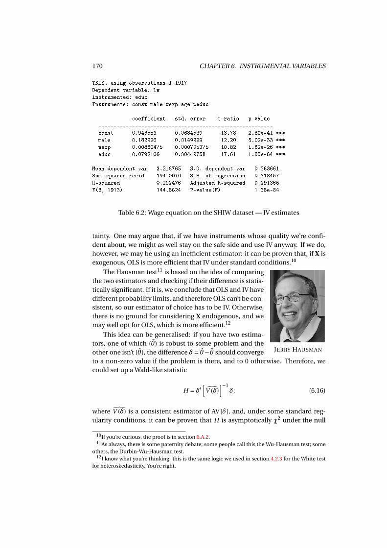
170 CHAPTER 6. INSTRUMENTAL VARIABLES
TSLS, using observations 1-1917
Dependent variable: lw
Instrumented: educ
Instruments: const male wexp age peduc
coefficient std. error t-ratio p-value
---------------------------------------------------------
const 0.943553 0.0684539 13.78 2.80e-41 ***
male 0.182926 0.0149929 12.20 5.02e-33 ***
wexp 0.00860475 0.000795375 10.82 1.62e-26 ***
educ 0.0792106 0.00449758 17.61 1.85e-64 ***
Mean dependent var 2.218765 S.D. dependent var 0.363661
Sum squared resid 194.0070 S.E. of regression 0.318457
R-squared 0.292476 Adjusted R-squared 0.291366
F(3, 1913) 144.8624 P-value(F) 1.38e-84
Table 6.2: Wage equation on the SHIW dataset — IV estimates
tainty. One may argue that, if we have instruments whose quality we’re confi-dent about, we might as well stay on the safe side and use IV anyway. If we do,however, we may be using an inefficient estimator: it can be proven that, if X isexogenous, OLS is more efficient that IV under standard conditions.10
JERRY HAUSMAN
The Hausman test11 is based on the idea of comparingthe two estimators and checking if their difference is statis-tically significant. If it is, we conclude that OLS and IV havedifferent probability limits, and therefore OLS can’t be con-sistent, so our estimator of choice has to be IV. Otherwise,there is no ground for considering X endogenous, and wemay well opt for OLS, which is more efficient.12
This idea can be generalised: if you have two estima-tors, one of which (θ) is robust to some problem and theother one isn’t (θ), the difference δ= θ− θ should convergeto a non-zero value if the problem is there, and to 0 otherwise. Therefore, wecould set up a Wald-like statistic
H = δ′[V (δ)
]−1δ; (6.16)
where V (δ) is a consistent estimator of AV[δ], and, under some standard reg-ularity conditions, it can be proven that H is asymptotically χ2 under the null
10If you’re curious, the proof is in section 6.A.2.11As always, there is some paternity debate; some people call this the Wu-Hausman test; some
others, the Durbin-Wu-Hausman test.12I know what you’re thinking: this is the same logic we used in section 4.2.3 for the White test
for heteroskedasticity. You’re right.
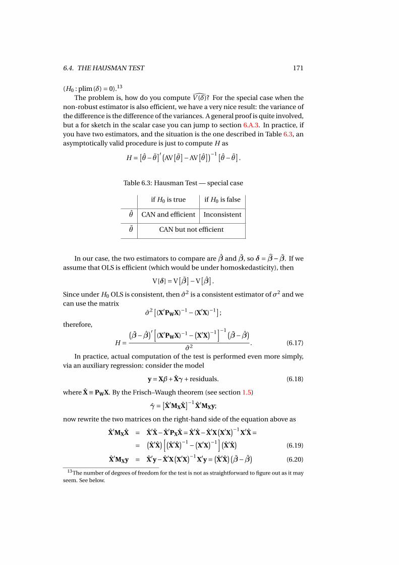
6.4. THE HAUSMAN TEST 171
(H0 : plim(δ) = 0).13
The problem is, how do you compute V (δ)? For the special case when thenon-robust estimator is also efficient, we have a very nice result: the variance ofthe difference is the difference of the variances. A general proof is quite involved,but a for sketch in the scalar case you can jump to section 6.A.3. In practice, ifyou have two estimators, and the situation is the one described in Table 6.3, anasymptotically valid procedure is just to compute H as
H = [θ− θ]′ (
AV[θ]−AV
[θ])−1 [
θ− θ].
Table 6.3: Hausman Test — special case
if H0 is true if H0 is false
θ CAN and efficient Inconsistent
θ CAN but not efficient
In our case, the two estimators to compare are β and β, so δ = β− β. If weassume that OLS is efficient (which would be under homoskedasticity), then
V[δ] = V[β
]−V[β
].
Since under H0 OLS is consistent, then σ2 is a consistent estimator of σ2 and wecan use the matrix
σ2 [(X′PWX)−1 − (X′X)−1] ;
therefore,
H =(β− β)′ [
(X′PWX)−1 − (X′X
)−1]−1 (
β− β)σ2 . (6.17)
In practice, actual computation of the test is performed even more simply,via an auxiliary regression: consider the model
y = Xβ+ Xγ+ residuals. (6.18)
where X ≡ PWX. By the Frisch–Waugh theorem (see section 1.5)
γ = [X′MXX
]−1X′MXy;
now rewrite the two matrices on the right-hand side of the equation above as
X′MXX = X′X− X′PXX = X′X− X′X(X′X
)−1 X′X == (
X′X)[(
X′X)−1 − (
X′X)−1
](X′X
)(6.19)
X′MXy = X′y− X′X(X′X
)−1 X′y = (X′X
)(β− β)
(6.20)
13The number of degrees of freedom for the test is not as straightforward to figure out as it mayseem. See below.
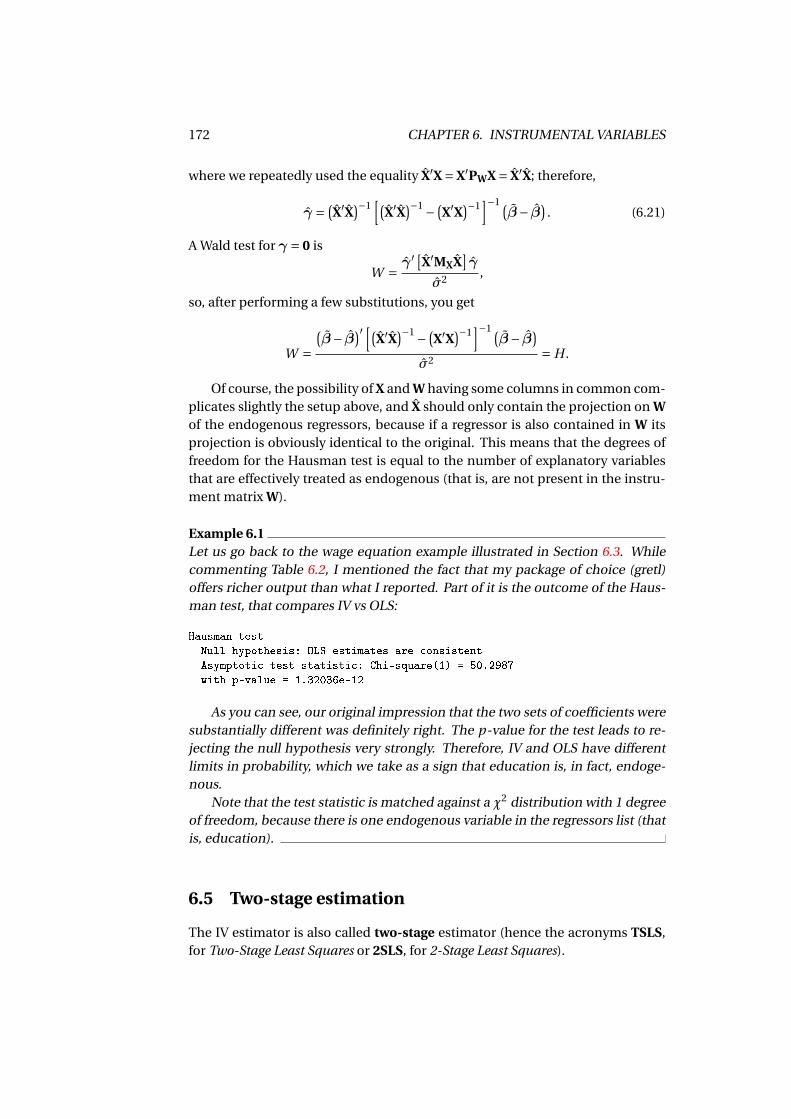
172 CHAPTER 6. INSTRUMENTAL VARIABLES
where we repeatedly used the equality X′X = X′PWX = X′X; therefore,
γ = (X′X
)−1[(
X′X)−1 − (
X′X)−1
]−1 (β− β)
. (6.21)
A Wald test for γ = 0 is
W = γ′ [X′MXX
]γ
σ2 ,
so, after performing a few substitutions, you get
W =(β− β)′ [(
X′X)−1 − (
X′X)−1
]−1 (β− β)
σ2 = H .
Of course, the possibility of X and W having some columns in common com-plicates slightly the setup above, and X should only contain the projection on Wof the endogenous regressors, because if a regressor is also contained in W itsprojection is obviously identical to the original. This means that the degrees offreedom for the Hausman test is equal to the number of explanatory variablesthat are effectively treated as endogenous (that is, are not present in the instru-ment matrix W).
Example 6.1Let us go back to the wage equation example illustrated in Section 6.3. Whilecommenting Table 6.2, I mentioned the fact that my package of choice (gretl)offers richer output than what I reported. Part of it is the outcome of the Haus-man test, that compares IV vs OLS:
Hausman test -
Null hypothesis: OLS estimates are consistent
Asymptotic test statistic: Chi-square(1) = 50.2987
with p-value = 1.32036e-12
As you can see, our original impression that the two sets of coefficients weresubstantially different was definitely right. The p-value for the test leads to re-jecting the null hypothesis very strongly. Therefore, IV and OLS have differentlimits in probability, which we take as a sign that education is, in fact, endoge-nous.
Note that the test statistic is matched against a χ2 distribution with 1 degreeof freedom, because there is one endogenous variable in the regressors list (thatis, education).
6.5 Two-stage estimation
The IV estimator is also called two-stage estimator (hence the acronyms TSLS,for Two-Stage Least Squares or 2SLS, for 2-Stage Least Squares).
6.5. TWO-STAGE ESTIMATION 173
The reason is that the β statistic may be computed by two successive ap-plications of OLS, called the two “stages”.14 In the era when computation wasexpensive, this was a nice trick to calculate β without the need for other soft-ware than OLS, but seeing IV as the product of a two-stage procedure has otheradvantages too.
In order to see what the two stages are, define X = PWX and rewrite (6.14) asfollows:
β = (X′X)−1X′y, (6.22)
The matrix X contains, in the j -th column, the fitted value of a regression of thej -th column of X on W; the regression
xi =Πwi +ui (6.23)
is what we call the first stage regression. In the second stage, you just regress yon X: the OLS coefficient equals β. Note: this is a numerically valid procedurefor computing β, but the standard errors you get are not valid for inference. Thisis because second stage residuals are e = y− Xβ, which is a different vector fromthe IV residuals ε= y−Xβ. Consequently, the statistic e′e
n does not provide a validestimator of σ2, which in turn makes the estimated covariance matrix invalid.
So, if the only computing facility you have is OLS (which was often the casein the 1950s and 1960s), you can compute the IV estimator via a repeated appli-cation of OLS. Moreover, you don’t really have to run as many first-stage regres-sions as the number of regressors. You just have to run one first-stage regressionfor each endogenous element of X (recall the discussion in subsection 6.4 on thedegrees of freedom for the Hausman test).
Example 6.2Let’s estimate the same model we used in section 6.3 via the two-stage method:the output from the first stage regression is in Table 6.4: as you can see, the de-pendent variable here is education, while the explanatory variables are the fullinstrument matrix W. There is not much to say about the first stage regression,except noting that the two “real” instruments (age and parents’ education) areboth highly significant. This will be important in the context of weak instru-ments (see section 6.7.2).
Once the first stage regression is computed, we save the fitted values intoa new variable called hat_educ. Then, we replace the original education educ
variable with hat_educ in the list of regressors and perform the second stage.Results are in Table 6.5; a comparison of these results with those reported inTable 6.2 reveals that:
1. the coefficients are identical;
14In fact, the word Henri Theil used when he invented this method was “rounds”, but subse-quent literature has settled on “stages”.
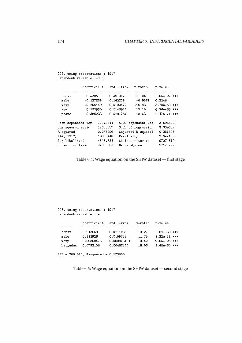
174 CHAPTER 6. INSTRUMENTAL VARIABLES
OLS, using observations 1-1917
Dependent variable: educ
coefficient std. error t-ratio p-value
---------------------------------------------------------
const 5.43051 0.491957 11.04 1.65e-27 ***
male -0.137838 0.142828 -0.9651 0.3346
wexp -0.205149 0.0129572 -15.83 3.78e-53 ***
age 0.192950 0.0146614 13.16 6.26e-38 ***
peduc 0.386233 0.0207287 18.63 2.47e-71 ***
Mean dependent var 11.73344 S.D. dependent var 3.598508
Sum squared resid 17665.37 S.E. of regression 3.039607
R-squared 0.287996 Adjusted R-squared 0.286507
F(4, 1912) 193.3448 P-value(F) 2.6e-139
Log-likelihood -4848.785 Akaike criterion 9707.570
Schwarz criterion 9735.363 Hannan-Quinn 9717.797
Table 6.4: Wage equation on the SHIW dataset — first stage
OLS, using observations 1-1917
Dependent variable: lw
coefficient std. error t-ratio p-value
---------------------------------------------------------
const 0.943553 0.0711035 13.27 1.64e-38 ***
male 0.182926 0.0155733 11.75 8.22e-31 ***
wexp 0.00860475 0.000826161 10.42 9.55e-25 ***
hat_educ 0.0792106 0.00467166 16.96 3.48e-60 ***
SSR = 209.316, R-squared = 0.173936
Table 6.5: Wage equation on the SHIW dataset — second stage
6.5. TWO-STAGE ESTIMATION 175
2. the standard error are not, because the statistic you obtain by dividing theSSR from the second-stage regression (209.316) by the number of obser-vations (1917) is not a consistent estimator for σ2; therefore, the standarderrors reported in table 6.5 differ from the correct ones by a constant scalefactor (1.0387 in this case).
6.5.1 The control function approach
The method I described in the previous subsection to compute the IV estimatorvia two successive stages is the traditional one. A slight variation on that proce-dure gives rise to what is sometimes called the control function approach.
The main idea can be grasped by considering a minimal model such as
yi = xi ·β+εi (6.24)
xi = wi ·π+ui , (6.25)
where equation (6.25) is a “proper” linear model, and Cov[ui ,εi ] is some realnumber, not necessarily 0. If wi is exogenous, the only way xi can be correlatedwith εi is if Cov[ui ,εi ] 6= 0. It is easy to show that OLS will overestimate β ifCov[ui ,εi ] > 0 and underestimate it if Cov[ui ,εi ] < 0. If, however, we defined
νi = εi −E[εi |ui ]
and assumed linearity of E[εi |ui ], we could write εi = ui ·θ+νi and recast (6.24)as
yi = xi ·β+ui ·θ+νi (6.26)
If we could observe ui , we wouldn’t need the IV estimator at all, because νi ,isorthogonal to both xi and ui ,15 so OLS would be our tool of choice.
Unfortunately, we don’t observe ui directly, but once we’ve run the first stageregression (6.25), we have the first-stage residuals ui , which hopefully shouldn’tbe too different; the possibility of using those in place of the “true” ui is tempt-ing.
From a computational point of view, hence, the control function approachdiffers from the traditional two-stage method only in the second stage. Once youhave performed the first stage, you use, in the second stage, the residuals fromthe first stage and add them as extra explanatory variables to the main equation.Call E the first-stage residuals and perform an OLS regression of y on X and Etogether:
y = Xβ+Eθ+ν; (6.27)
the estimates we get have a very nice interpretation.
15Lazy writers like myself love the sentence: “the proof is left to the reader as an exercise”.
176 CHAPTER 6. INSTRUMENTAL VARIABLES
Let’s begin with β: by the Frisch-Waugh theorem, the coefficient vector as-sociated with X is
(X′MEX)−1X′MEy;
now focus on the matrix X′ME:
X′ME = X′−X′PE = X′−X′E(E′E)−1E′.
Since, by definition, E = MWX, by substitution we have
X′ME = X′−X′MWX(X′MWX)−1X′MW = X′−X′MW = X′PW;
therefore, the coefficient vector becomes
(X′MEX)−1X′MEy = (X′PWX)−1X′PWy = β
So the OLS estimate of the coefficients associated with X in equation (6.27)is exactly equal to the IV estimator β. Warning: the reader should be aware that,just like the two-stage procedure, the control function approach does not yieldcorrect standard errors for β; explaining precisely why is far beyond the scope ofthis book, and readers will have to content themselves with knowing that this isa consequence of using the first-stage residuals ui in place of the true ui series.16
Moreover, the control function regression gives you, as a nice by-product,the Hausman test, as an exclusion test for the first-stage residuals: by applyingthe Frisch-Waugh theorem again, the OLS estimate of θ in (6.27) is
θ = [E′MXE
]−1 E′MXy;
of course e = MXy are the OLS residuals. Now use the definition of E as E = MWXagain:
E′MXy = E′e = X′MWe = X′e−X′PWe =−X′PWe;
where the last equality comes from the OLS residuals e being orthogonal to X;therefore
E′MXy =−X′PWy+X′PWX · β = [X′PWX
](β− β),
and as a consequence θ is just
θ = [E′MXE
]−1 [X′PWX
](β− β);
since the matrix[E′MXE
]−1 [X′PWX
]is invertible, θ it can be zero if and only if
β = β. Therefore, the hypothesis h0 : θ = 0 is logically equivalent to the nullhypothesis of the Hausman test, and the test can be performed a a simple zero
16If you really want to know, this is a case of generated regressors; section 6.1 of Wooldridge(2010) is where you want to start from. Besides, Section 6.2 of the same book contains a muchmore accurate and thorough treatment of the control function approach than what I’m givingyou here.
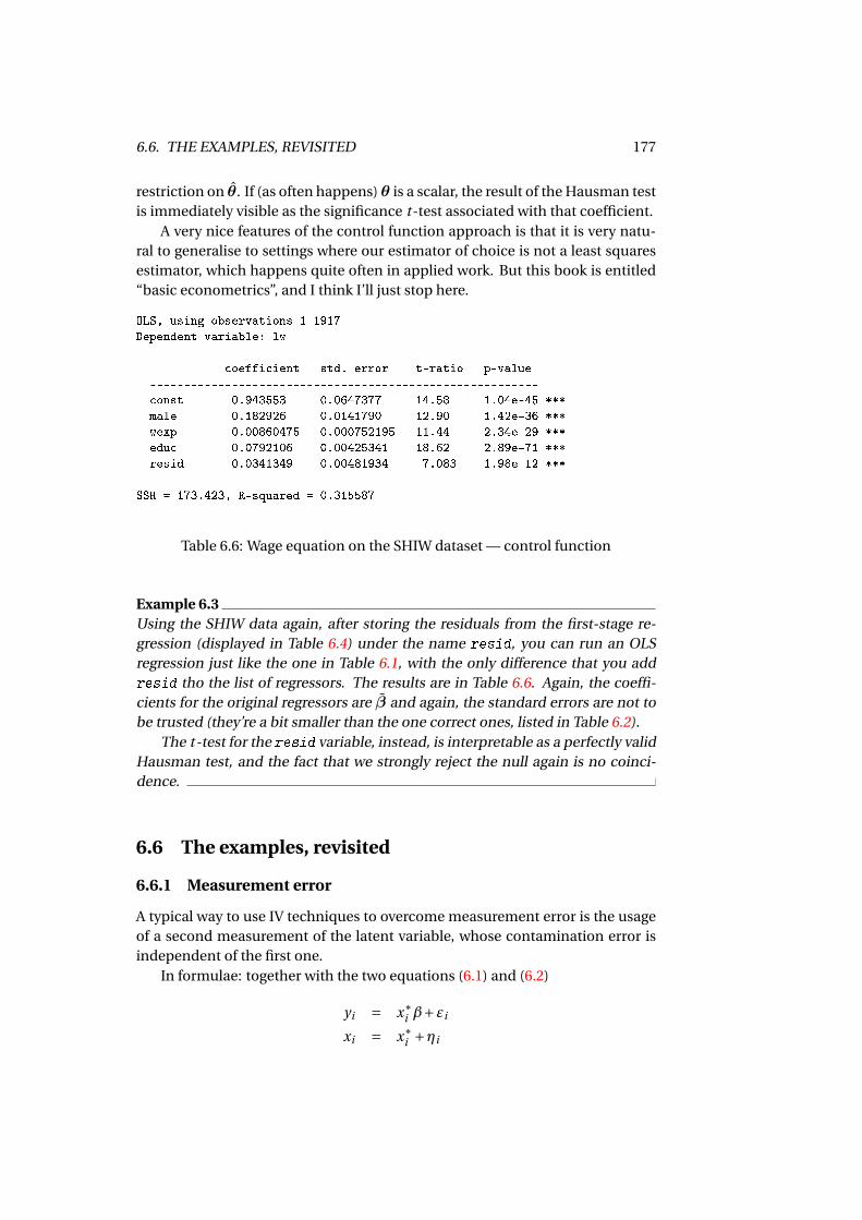
6.6. THE EXAMPLES, REVISITED 177
restriction on θ. If (as often happens) θ is a scalar, the result of the Hausman testis immediately visible as the significance t-test associated with that coefficient.
A very nice features of the control function approach is that it is very natu-ral to generalise to settings where our estimator of choice is not a least squaresestimator, which happens quite often in applied work. But this book is entitled“basic econometrics”, and I think I’ll just stop here.
OLS, using observations 1-1917
Dependent variable: lw
coefficient std. error t-ratio p-value
---------------------------------------------------------
const 0.943553 0.0647377 14.58 1.04e-45 ***
male 0.182926 0.0141790 12.90 1.42e-36 ***
wexp 0.00860475 0.000752195 11.44 2.34e-29 ***
educ 0.0792106 0.00425341 18.62 2.89e-71 ***
resid -0.0341349 0.00481934 -7.083 1.98e-12 ***
SSR = 173.423, R-squared = 0.315587
Table 6.6: Wage equation on the SHIW dataset — control function
Example 6.3Using the SHIW data again, after storing the residuals from the first-stage re-gression (displayed in Table 6.4) under the name resid, you can run an OLSregression just like the one in Table 6.1, with the only difference that you addresid tho the list of regressors. The results are in Table 6.6. Again, the coeffi-cients for the original regressors are β and again, the standard errors are not tobe trusted (they’re a bit smaller than the one correct ones, listed in Table 6.2).
The t-test for the resid variable, instead, is interpretable as a perfectly validHausman test, and the fact that we strongly reject the null again is no coinci-dence.
6.6 The examples, revisited
6.6.1 Measurement error
A typical way to use IV techniques to overcome measurement error is the usageof a second measurement of the latent variable, whose contamination error isindependent of the first one.
In formulae: together with the two equations (6.1) and (6.2)
yi = x∗i β+εi
xi = x∗i +ηi
178 CHAPTER 6. INSTRUMENTAL VARIABLES
suppose you have a third observable variable wi such that
wt = x∗t +νt
It can be proven that, if ηt and νt are uncorrelated, then wt is a valid instrumentand the statistic
β=∑
wt yt∑wt xt
is consistent for β.One famous application of this principle is provided in Griliches (1976), a
landmark article in labour economics, where the author has two measurementsof individual ability and uses one for instrumenting the other.
6.6.2 Simultaneous equation systems
Consider again equations (6.4)–(6.5):
qt = α0 −α1pt +ut
pt = β0 +β1qt + vt .
As we proved in section 6.1.2, the systematic part of these two equations are notconditional means, so there’s no way we can estimate their parameters consis-tently via OLS.
On the other hand, we can use (6.7) to deduce that E[pt
] = π1; clearly, theparameter π1 can be estimated consistently very simply by taking the average ofpt (or regressing pt on a constant, if you will). The same holds for E
[qt
]=π0.Can we use these two parameters to estimate the structural ones? The an-
swer is no: the relationship between the (π0,π1) pair and the structural parame-ters is
π0 = α0 −β0α1
1+β1α1π1 = β0 +β1α0
1+β1α1,
which is a system of 2 equations in 4 unknowns; as such, it has infinitely manysolutions. This is exactly the under-identification scenario we analysed in sec-tion 2.5.
Let us now consider this example in greater generality: a system of linearequations can be written as
Γyt = Bxt +εt ; (6.28)
the yt vector contains the q endogenous variables, while xt is an m-vector hold-ing the exogenous variables. The matrix Γ (assumed non-singular) is q ×q andB is a q ×m matrix. In the demand-supply example,
Γ=[
1 α1
−β1 1
]B =
[α0
β0
].
Equation (6.28) is known as the structural form of the system, because its pa-rameters have a behavioural interpretation and are our parameters of interest.
6.7. ARE MY INSTRUMENTS OK? 179
By pre-multiplying (6.28) by Γ−1, you get the so-called reduced form:
yt =Πxt +ut , (6.29)
whereΠ= Γ−1B and ut = Γ−1εt . In our example, the matrixΠ is a column vector,containing π0 and π1.
If xt is exogenous, then Cov[xt ,εt ], so the correlation between xt and ut iszero; hence, OLS is a consistent estimator for the parameters of the reducedform. However, by postmultiplying (6.29) by x′t you get:
yt x′t =Πxt x′t +ut x′t ,
which implies E[yt x′t
] = ΠE[xt x′t
]. Ordinarily, this matrix should not contain
zeros; if variables were centred in mean, it would be the covariance matrix be-tween the vector yt and the vector xt . Therefore, each element of xt is correlatedwith each yt despite being uncorrelated with εt . In other words, xt is both rele-vant and exogenous and, as such, is a perfect instrument.
In the example above, xt contains only the constant term, and the reducedform looks like: [
qt
pt
]=
[π0
π1
]·1+ut ;
it should be clear where under-identification comes from: in the demand equa-tion you have 2 regressors (the constant and pt ) but only one instrument (theconstant), and the same goes, mutatis mutandis, for the supply equation.
Consider now a different formulation, where:
qt = α0 −α1pt +α2 yt +ut (6.30)
pt = β0 +β1qt +β2mt + vt , (6.31)
and the two new variables (both assumed exogenous) are:
yt per capita income at time tmt price of raw materials at time t
In this case, both equations are estimable via IV, because we have three re-gressors and three instruments for each (the same for both: constant, yt andmt ). In the context of simultaneous systems, the order condition I stated in sec-tion 6.2.2 is often translated as: for each equation in the system the number ofincluded endogenous variables cannot be greater than the number of excludedexogenous variables. I’ll leave it to the reader to work out the equivalence.
6.7 Are my instruments OK?
A fundamental requirement for the whole IV strategy is that the variables that wechoose to use as instruments are (i) exogenous and (ii) relevant. It goes without
180 CHAPTER 6. INSTRUMENTAL VARIABLES
saying that we cannot just assume that they are just because we say so, and it’dbe nice to have some way of testing these assumptions.
It turns out that neither property can be verified directly, but we do havestatistics that we can interpret in a useful way.
6.7.1 The Sargan test
The Sargan test is often interpreted as a test for exogeneity of the instruments,but in fact things are a little bit more subtle.
Exogeneity, in our context, means uncorrelatedness between the instrumentswi and the structural disturbances εi . If the latter were observable, a test wouldbe straightforward to construct: under H0,
1pn
W′ε d−→ N(0, σ2W′W
)and it can be proven that, under H0,
ε′PWε
σ2d−→χ2
m , (6.32)
where m is the size of wi . Unfortunately, ε is unobservable, and therefore thequantity above is not a statistic and cannot be used as a test.
The idea of substituting disturbances with residuals like we did in section6.5.1 takes us to the Sargan test. Its most important feature is that this test hasa different asymptotic distribution than (6.32), since the degrees of freedom ofthe limit χ2 is not m (the number of instruments), but rather m −k, where k isthe number of elements in β: in other terms, the over-identification rank (seesection 6.2.1). In formulae,
S = ε′PWε
σ2d−→χ2
m−k . (6.33)
This result may appear surprising at first. Consider, however, that under ex-act identification the numerator of S is identically zero,17 so, in turn, the S statis-tic is identically 0, not a χ2
m variable. Can this result be generalised?Consider the conditional expectation E
[yi |wi
]; assuming linearity, if wi is
exogenous we could estimate its parameters via OLS in a model like
yi = w′iπ+ui ; (6.34)
in the simultaneous system jargon, equation (6.34) would be the reduced-formequation for yi . To see how the parameters π relate to β, write the first-stageequation (6.25) in matrix form as
X = WΠ+E17Blitz proof: if m = k, then β = (W′X)−1W′y. Therefore, PWε = PW(y−Xβ); however, observe
that PWXβ = W′(W′W)−1W′X(W′X)−1W′y = PWy. As a consequence, PWε= PWy−PWy = 0.
6.7. ARE MY INSTRUMENTS OK? 181
so that the i -th row of X can be written as x′i = w′iΠ+ e′i ; now substitute in the
structural equation:
yi = x′iβ+εi = w′iΠβ+ (εi +e′iβ); (6.35)
clearly, the two models (6.34) and (6.35) become equivalent only if π =Πβ; infact, the expressionΠβ can be seen as a restricted version of π, where the con-straint is that π must be a linear combination of the columns of Π (or, moreconcisely, that π ∈ Sp(Π)).
The Sargan test is precisely a test for those restrictions: this begs three ques-tions:
1. how do we compute the test statistic?
2. What is its limit distribution?
3. Which interpretation must be given to a rejection?
Number 1 is quite easy: the IV residuals ε are the residuals from the restrictedmodel. All we have to do is apply the LM principle (see Section 3.6.1) and regressthose on the explanatory variables from the unrestricted model. Compute nR2,and your job is done. If you do, you end up exactly with the statistic I called S inequation (6.33).
As for its limit distribution, I will now prove that the number of degrees offreedom of the χ2 limit distribution is m−k: if the restriction is true, then PΠπ =π, or, equivalently, MΠπ = 0. Since the rank of MΠ is m −k, we can write
MΠπ =UV ′π = 0
where V and U are matrices with k rows and m −k columns (see section 1.A.3).So, the null hypothesis implicit in the restriction is H0 : V ′π = 0, which is a sys-tem of m − r constraints.
Now we can tackle point 3: the null hypothesis in the Sargan test is that them relationships implicit in the equation π =Πβ are non-contradictory; if theywere, it would mean that at least one element of the vector E[wiεi ] is non-zero,and therefore at least one instrument in not exogenous. Unfortunately, the testcannot identify the culprit.
To clarify the matter, take for example a simple DGP where yi = xiβ+εi andwe have two potential instruments, w1,i and w2,i . We can choose among threepossible IV estimators for β:
• a simple IV estimator using w1,i only (call it β1);
• a simple IV estimator using w2,i only (call it β2);
• the GIVE estimator using both w1,i and w2,i (call it β12).
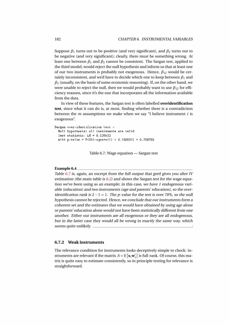
182 CHAPTER 6. INSTRUMENTAL VARIABLES
Suppose β1 turns out to be positive (and very significant), and β2 turns out tobe negative (and very significant); clearly, there must be something wrong. Atleast one between β1 and β2 cannot be consistent. The Sargan test, applied tothe third model, would reject the null hypothesis and inform us that at least oneof our two instruments is probably not exogenous. Hence, β12 would be cer-tainly inconsistent, and we’d have to decide which one to keep between β1 andβ2 (usually, on the basis of some economic reasoning). If, on the other hand, wewere unable to reject the null, then we would probably want to use β12 for effi-ciency reasons, since it’s the one that incorporates all the information availablefrom the data.
In view of these features, the Sargan test is often labelled overidentificationtest, since what it can do is, at most, finding whether there is a contradictionbetween the m assumptions we make when we say “I believe instrument i isexogenous”.
Sargan over-identification test -
Null hypothesis: all instruments are valid
Test statistic: LM = 0.138522
with p-value = P(Chi-square(1) > 0.138522) = 0.709755
Table 6.7: Wage equation — Sargan test
Example 6.4Table 6.7 is, again, an excerpt from the full output that gretl gives you after IVestimation (the main table is 6.2) and shows the Sargan test for the wage equa-tion we’ve been using as an example; in this case, we have 1 endogenous vari-able (education) and two instruments (age and parents’ education), so the over-identification rank is 2−1 = 1. The p-value for the test is over 70%, so the nullhypothesis cannot be rejected. Hence, we conclude that our instruments form acoherent set and the estimates that we would have obtained by using age aloneor parents’ education alone would not have been statistically different from oneanother. Either our instruments are all exogenous or they are all endogenous,but in the latter case they would all be wrong in exactly the same way, whichseems quite unlikely.
6.7.2 Weak instruments
The relevance condition for instruments looks deceptively simple to check: in-struments are relevant if the matrix A = E
[xi w′
i
]is full-rank. Of course, this ma-
trix is quite easy to estimate consistently, so in principle testing for relevance isstraightforward.
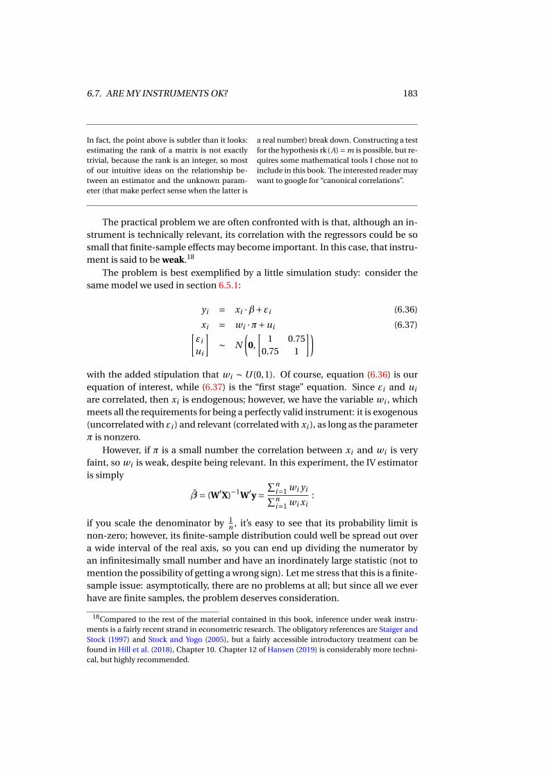
6.7. ARE MY INSTRUMENTS OK? 183
In fact, the point above is subtler than it looks:estimating the rank of a matrix is not exactlytrivial, because the rank is an integer, so mostof our intuitive ideas on the relationship be-tween an estimator and the unknown param-eter (that make perfect sense when the latter is
a real number) break down. Constructing a testfor the hypothesis rk(A) = m is possible, but re-quires some mathematical tools I chose not toinclude in this book. The interested reader maywant to google for “canonical correlations”.
The practical problem we are often confronted with is that, although an in-strument is technically relevant, its correlation with the regressors could be sosmall that finite-sample effects may become important. In this case, that instru-ment is said to be weak.18
The problem is best exemplified by a little simulation study: consider thesame model we used in section 6.5.1:
yi = xi ·β+εi (6.36)
xi = wi ·π+ui (6.37)[εi
ui
]∼ N
(0,
[1 0.75
0.75 1
])with the added stipulation that wi ∼ U (0,1). Of course, equation (6.36) is ourequation of interest, while (6.37) is the “first stage” equation. Since εi and ui
are correlated, then xi is endogenous; however, we have the variable wi , whichmeets all the requirements for being a perfectly valid instrument: it is exogenous(uncorrelated with εi ) and relevant (correlated with xi ), as long as the parameterπ is nonzero.
However, if π is a small number the correlation between xi and wi is veryfaint, so wi is weak, despite being relevant. In this experiment, the IV estimatoris simply
β = (W′X)−1W′y =∑n
i=1 wi yi∑ni=1 wi xi
:
if you scale the denominator by 1n , it’s easy to see that its probability limit is
non-zero; however, its finite-sample distribution could well be spread out overa wide interval of the real axis, so you can end up dividing the numerator byan infinitesimally small number and have an inordinately large statistic (not tomention the possibility of getting a wrong sign). Let me stress that this is a finite-sample issue: asymptotically, there are no problems at all; but since all we everhave are finite samples, the problem deserves consideration.
18Compared to the rest of the material contained in this book, inference under weak instru-ments is a fairly recent strand in econometric research. The obligatory references are Staiger andStock (1997) and Stock and Yogo (2005), but a fairly accessible introductory treatment can befound in Hill et al. (2018), Chapter 10. Chapter 12 of Hansen (2019) is considerably more techni-cal, but highly recommended.
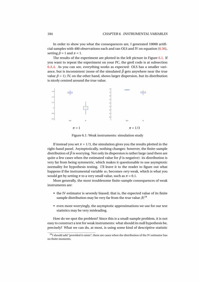
184 CHAPTER 6. INSTRUMENTAL VARIABLES
In order to show you what the consequences are, I generated 10000 artifi-cial samples with 400 observations each and ran OLS and IV on equation (6.36),setting β= 1 and π= 1.
The results of the experiment are plotted in the left picture in Figure 6.1. Ifyou want to repeat the experiment on your PC, the gretl code is at subsection6.A.4. As you can see, everything works as expected: OLS has a smaller vari-ance, but is inconsistent (none of the simulated β gets anywhere near the truevalue β = 1); IV, on the other hand, shows larger dispersion, but its distributionis nicely centred around the true value.
0.6
0.8
1
1.2
1.4
1.6
OLS IV
-6
-5
-4
-3
-2
-1
0
1
2
OLS IV
π= 1 π= 1/3
Figure 6.1: Weak instruments: simulation study
If instead you set π= 1/3, the simulation gives you the results plotted in theright-hand panel. Asymptotically, nothing changes: however, the finite-sampledistribution of β is worrying. Not only its dispersion is rather large (and there arequite a few cases when the estimated value for β is negative): its distribution isvery far from being symmetric, which makes it questionable to use asymptoticnormality for hypothesis testing. I’ll leave it to the reader to figure out whathappens if the instrumental variable wi becomes very weak, which is what youwould get by setting π to a very small value, such as π= 0.1.
More generally, the most troublesome finite-sample consequences of weakinstruments are:
• the IV estimator is severely biased; that is, the expected value of its finitesample distribution may be very far from the true value β;19
• even more worryingly, the asymptotic approximations we use for our teststatistics may be very misleading.
How do we spot the problem? Since this is a small-sample problem, it is noteasy to construct a test for weak instruments: what should its null hypothesis be,precisely? What we can do, at most, is using some kind of descriptive statistic
19I should add “provided it exists”; there are cases when the distribution of the IV estimator hasno finite moments.
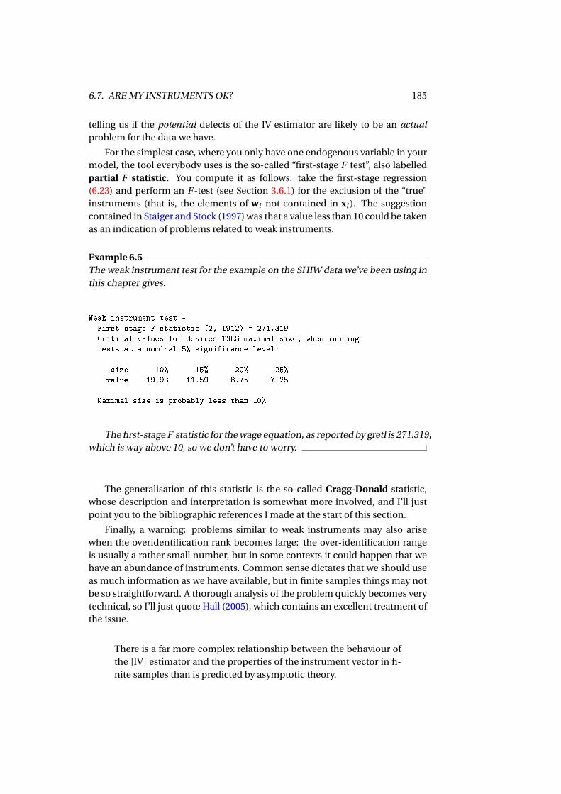
6.7. ARE MY INSTRUMENTS OK? 185
telling us if the potential defects of the IV estimator are likely to be an actualproblem for the data we have.
For the simplest case, where you only have one endogenous variable in yourmodel, the tool everybody uses is the so-called “first-stage F test”, also labelledpartial F statistic. You compute it as follows: take the first-stage regression(6.23) and perform an F -test (see Section 3.6.1) for the exclusion of the “true”instruments (that is, the elements of wi not contained in xi ). The suggestioncontained in Staiger and Stock (1997) was that a value less than 10 could be takenas an indication of problems related to weak instruments.
Example 6.5The weak instrument test for the example on the SHIW data we’ve been using inthis chapter gives:
Weak instrument test -
First-stage F-statistic (2, 1912) = 271.319
Critical values for desired TSLS maximal size, when running
tests at a nominal 5% significance level:
size 10% 15% 20% 25%
value 19.93 11.59 8.75 7.25
Maximal size is probably less than 10%
The first-stage F statistic for the wage equation, as reported by gretl is 271.319,which is way above 10, so we don’t have to worry.
The generalisation of this statistic is the so-called Cragg-Donald statistic,whose description and interpretation is somewhat more involved, and I’ll justpoint you to the bibliographic references I made at the start of this section.
Finally, a warning: problems similar to weak instruments may also arisewhen the overidentification rank becomes large: the over-identification rangeis usually a rather small number, but in some contexts it could happen that wehave an abundance of instruments. Common sense dictates that we should useas much information as we have available, but in finite samples things may notbe so straightforward. A thorough analysis of the problem quickly becomes verytechnical, so I’ll just quote Hall (2005), which contains an excellent treatment ofthe issue.
There is a far more complex relationship between the behaviour ofthe [IV] estimator and the properties of the instrument vector in fi-nite samples than is predicted by asymptotic theory.
186 CHAPTER 6. INSTRUMENTAL VARIABLES
6.A Assorted results
6.A.1 Asymptotic properties of the IV estimator
The limit in probability of the IV estimator (see 6.2.1 for its derivation)
β = (X′PWX)−1X′PWy,
can be calculated by rewriting the equation above as a function of statistics forwhich the probability limits can be computed easily. Clearly, some regularityconditions (such as the observations being iid, for example) are assumed to holdso that convergence occurs; we’ll take these as given and assume that samplemoments converge in probability to the relevant moments.
Given the linear model yi = x′iβ+εi , we assume that:
1. 1n
∑Tt=1 xt w′
t = X′Wn
p−→ A, where rk(A) = k;
2. 1n
∑Tt=1 wt w′
t = W′Wn
p−→ B , where B is invertible;
3. 1n
∑Tt=1 wt ut = W′ε
np−→ 0;
then β = (X′PWX)−1X′PWyp−→ β. The proof is a simple application of Slutsky’s
theorem:
β = β+ (X′PWX)−1X′PWε=
= β+[(
X′Wn
)(W′W
n
)−1 (W′X
n
)]−1 (X′W
n
)(W′W
n
)−1 (W′ε
n
)so that
βp−→β+ [
AB−1 A′]−1AB−1 ·0 =β. (6.38)
It is instructive to consider the role played by the ranks of A and B ; the matrixB must be invertible, because otherwise AB−1 A′ wouldn’t exist. Since B is theprobability limit of the second moments of the instruments, this requirement isequivalent to saying that all instruments must carry separate information, andcannot be collinear.
Note that the requisite is only that the instru-ments shouldn’t be collinear: the stronger req-uisite of independence is not needed. As aconsequence, it is perfectly OK to use nonlin-ear transformations of one instrument to createadditional ones.For example, if you have a variable wi thatyou assume independent of εi , you can useas instruments wi , w2
i , log(wi ), . . . (provided of
course that the transformed variables have fi-nite moments).This strategy is a special case of somethingcalled identification through nonlinearity; al-though it feels a bit like cheating (and isfrowned upon by some), it is perfectly legiti-mate, at least asymptotically, as long as eachtransformation carries some extra amount ofinformation.
6.A. ASSORTED RESULTS 187
The rank of A, instead, must be k for[
AB−1 A′] to be invertible. This meansthat instruments wi must be relevant (see Section 6.2.2) for all the regressorsxi . If
[AB−1 A′] is not invertible, then the probability limit in (6.38) does not
exist. If, instead, it’s invertible, but very close to being singular (as in the caseof weak instruments — see Section 6.7.2), then its inverse will be a matrix withinordinately large values. This is mainly a problem for the distribution of β: ifwe also assume
4. 1pn
∑Tt=1 wt ut = W′εp
n
d−→ N (0,Q);
thenp
n(β−β)d−→ N (0,Σ), where
Σ= [AB−1 A′]−1
AB−1QB−1 A′ [AB−1 A′]−1.
In the standard case Q =σ2B (from the homoskedasticity assumption E[εε′|W]=
σ2I), and therefore
pn(β−β)
d−→ N(0,σ2 [
AB−1 A′]−1)
. (6.39)
So the precision of the IV estimator is severely impaired any time the matrix[AB−1 A′] is close to being singular.
The last thing is proving that σ2 is consistent: from
ε= X(β− β)+ε,
you get
ε′ε= (β− β)′
X′X(β− β)+2
(β− β)′
X′ε+ε′ε
and therefore
1
nε′ε= (
β− β)′ (X′Xn
)(β− β)+2
(β− β)′ (X′ε
n
)+
(ε′εn
).
By taking probability limits,
σ2 = 1
nε′ε
p−→ 0′ (Q)0+2 ·0′λ+σ2 =σ2,
where Q = plim(
X′Xn
)and λ= plim
(X′εn
). Note that σ2 is consistent even though
λ 6= 0. Consistency of σ2 is important because it implies that we can use theempirical counterparts of the asymptotic covariance matrix in equation (6.39)and use σ2(X′PWX)−1 as a valid covariance matrix for Wald tests.
188 CHAPTER 6. INSTRUMENTAL VARIABLES
6.A.2 Proof that OLS is more efficient than IV
In the OLS vs IV case, the proof that OLS is more efficient than IV if X is exoge-nous can be given as follows: given the model yi = x′iβ+εi , define the followingquantities:
Q = plim
(X′Xn
)A = plim
(W′X
n
)B = plim
(W′W
n
);
under homoskedasticity, we have that AV[β
] = σ2Q−1 (see section 3.2.2) and
AV[β
] = σ2[
A′B−1 A]−1
(see 6.A.1), where σ2 = V[εi ]. In order to prove thatAV
[β
]−AV[β
]is positive semi-definite, we re-use two of the results on positive
definite matrices that we employed in section 4.A.3:
1. if Q and P are invertible and Q −P is psd, then P−1 −Q−1 is also psd;
2. if Q is psd, then P ′QP is also psd for any matrix P .
Begin by applying property 1 above and define
∆≡σ2 ·[
AV[β
]−1 −AV[β
]−1]=Q − A′B−1 A;
Since σ2 > 0, it is sufficient to prove that ∆ is psd. Now define the vector z′i =[x′i w′
i ] and consider the probability limit of its second moments:
C = plim
(Z′Zn
)=
[Q A′
A B
]where C is clearly psd; now define H as
H = [I −A′B−1
]so, by property 2, the product HC H ′ is also psd; but
HC H ′ = [I −A′B−1
][Q A′
A B
][I
−B−1 A
]=Q − A′B−1 A =∆,
and the proof is complete.
6.A.3 Covariance matrix for the Hausman test (scalar case)
Suppose we have two consistent estimators of a scalar parameter θ; call them θ
and θ; assume also that the joint asymptotic distribution of θ and θ is normal.Then,
AV
[θ
θ
]=
[a bb c
].
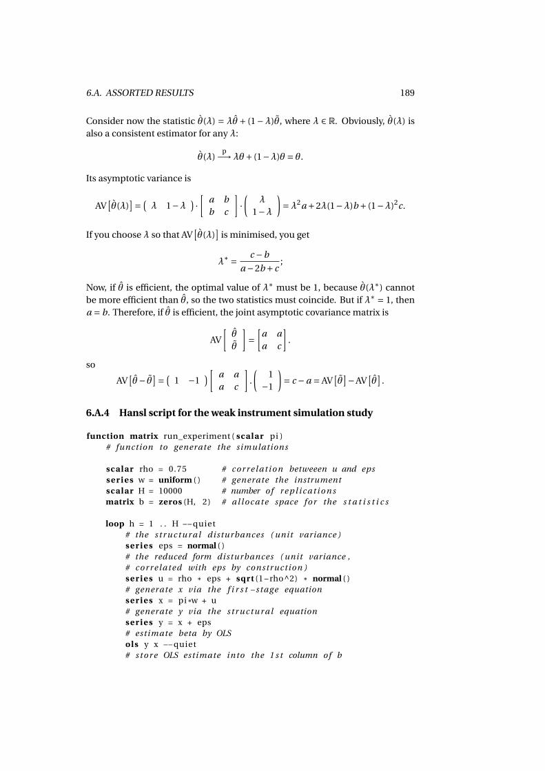
6.A. ASSORTED RESULTS 189
Consider now the statistic θ(λ) = λθ+ (1−λ)θ, where λ ∈ R. Obviously, θ(λ) isalso a consistent estimator for any λ:
θ(λ)p−→λθ+ (1−λ)θ = θ.
Its asymptotic variance is
AV[θ(λ)
]= (λ 1−λ ) ·[ a b
b c
]·(
λ
1−λ)=λ2a +2λ(1−λ)b + (1−λ)2c.
If you choose λ so that AV[θ(λ)
]is minimised, you get
λ∗ = c −b
a −2b + c;
Now, if θ is efficient, the optimal value of λ∗ must be 1, because θ(λ∗) cannotbe more efficient than θ, so the two statistics must coincide. But if λ∗ = 1, thena = b. Therefore, if θ is efficient, the joint asymptotic covariance matrix is
AV
[θ
θ
]=
[a aa c
].
so
AV[θ− θ]= (
1 −1)[ a a
a c
].
(1
−1
)= c −a = AV
[θ]−AV
[θ]
.
6.A.4 Hansl script for the weak instrument simulation study
function matrix run_experiment ( scalar pi )# function to generate the simulations
scalar rho = 0.75 # c o r r e l a t i o n betweeen u and epss e r i e s w = uniform ( ) # generate the instrumentscalar H = 10000 # number of r e p l i c a t i o n smatrix b = zeros (H, 2) # a l l o c a t e space f o r the s t a t i s t i c s
loop h = 1 . . H −−quiet# the s t r u c t u r a l disturbances ( unit variance )s e r i e s eps = normal ( )# the reduced form disturbances ( unit variance ,# c o r r e l a t e d with eps by construction )s e r i e s u = rho * eps + sqrt (1−rho^2) * normal ( )# generate x via the f i r s t −stage equations e r i e s x = pi *w + u# generate y via the s t r u c t u r a l equations e r i e s y = x + eps# estimate beta by OLSols y x −−quiet# s t o r e OLS estimate into the 1 s t column of b
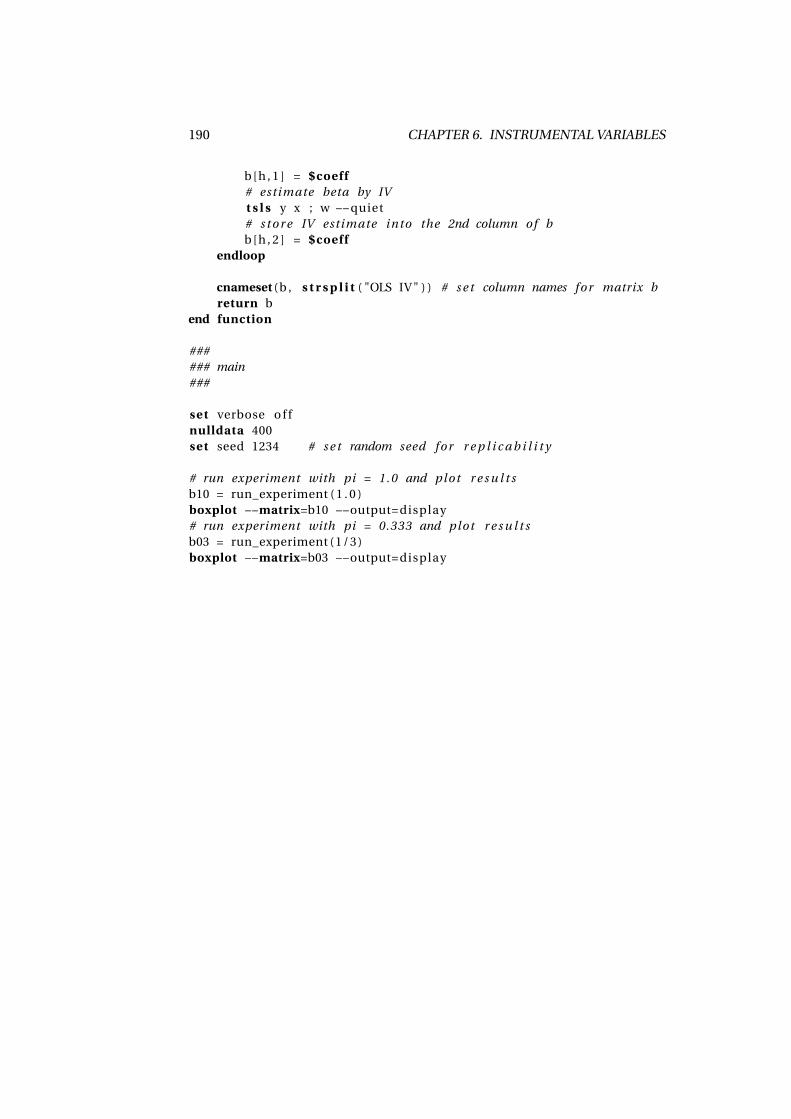
190 CHAPTER 6. INSTRUMENTAL VARIABLES
b[h , 1 ] = $coeff# estimate beta by IVt s l s y x ; w −−quiet# s t o r e IV estimate into the 2nd column of bb[h , 2 ] = $coeff
endloop
cnameset (b , s t r s p l i t ( "OLS IV " ) ) # s e t column names f o r matrix breturn b
end function
###### main###
set verbose o f fnulldata 400set seed 1234 # s e t random seed f o r r e p l i c a b i l i t y
# run experiment with pi = 1.0 and plot r e s u l t sb10 = run_experiment ( 1 . 0 )boxplot −−matrix=b10 −−output=display# run experiment with pi = 0.333 and plot r e s u l t sb03 = run_experiment (1/3)boxplot −−matrix=b03 −−output=display

Bibliography
ANDERSEN, H. AND B. HEPBURN (2016): “Scientific Method,” in The Stanford En-cyclopedia of Philosophy, ed. by E. N. Zalta, Metaphysics Research Lab, Stan-ford University, summer 2016 ed.
ANGRIST, J. D. AND J.-S. PISCHKE (2008): Mostly harmless econometrics: An em-piricist’s companion, Princeton University Press.
BIAU, D. J., B. M. JOLLES, AND R. PORCHER (2009): “P value and the theory ofhypothesis testing: an explanation for new researchers,” Clinical orthopaedicsand related research, 468, 885–892.
BIERENS, H. J. (2011): Introduction to the Mathematical and Statistical Founda-tions of Econometrics, Cambridge University Press.
BILLINGSLEY, P. (1986): Probability and Measure, Wiley series in probability andmathematical statistics, John Wiley and Sons, 2nd ed.
BROCKWELL, P. AND R. DAVIS (1991): Time Series: Theory and Methods, SpringerSeries in Statistics, Springer.
CAMERON, A. C. AND D. L. MILLER (2015): “A practitioner’s guide to cluster-robust inference,” Journal of Human Resources, 50, 317–372.
CAMERON, A. C. AND P. K. TRIVEDI (2005): Microeconometrics, Cambridge Uni-versity Press.
CARD, D. (1999): “The causal effect of education on earnings,” in Handbook ofLabor Economics, ed. by O. Ashenfelter and D. Card, Elsevier, vol. 3, Part A,chap. 30, 1801–1863, 1 ed.
CASELLA, G. AND R. L. BERGER (2002): Statistical inference, Duxbury PacificGrove, CA, 2nd ed.
DADKHAH, K. (2011): Foundations of mathematical and computational eco-nomics. 2nd ed., Berlin: Springer, 2nd ed. ed.
DAVIDSON, J. (1994): Stochastic limit theory: An introduction for econometri-cians, Oxford University Press.
191
192 BIBLIOGRAPHY
——— (2000): Econometric Theory, Wiley-Blackwell.
DAVIDSON, J., D. HENDRY, F. SRBA, AND S. YEO (1978): “Econometric Modellingof the Aggregate Time-Series Relationship between Consumers’ Expenditureand Income in the United Kingdom,” Economic Journal, 88, 661–92.
DAVIDSON, R. AND J. G. MACKINNON (1993): Estimation and inference in econo-metrics, Oxford University Press.
——— (2004): Econometric theory and methods, Oxford University Press NewYork.
DIXIT, A. K. (1990): Optimization in economic theory, Oxford University Press.
DURLAUF, S. AND L. BLUME (2008): The New Palgrave Dictionary of Economics,Palgrave Macmillan UK.
EFRON, B. AND T. HASTIE (2016): Computer Age Statistical Inference: Algorithms,Evidence, and Data Science, Cambridge University Press, 1st ed.
EPPERSON, J. F. (2013): An Introduction to Numerical Methods and Analysis, Wi-ley Publishing, 2nd ed.
FREEDMAN, D. AND P. STARK (2016): “What is the chance of an earthquake?”Tech. Rep. 611, Department of Statistics, University of California, Berkeley.
GALLANT, R. A. (1997): An Introduction to Econometric Theory, Princeton Uni-versity Press.
GALTON, F. (1886): “Regression Towards Mediocrity in Hereditary Stature,” Jour-nal of the Anthropological Institute of Great Britain and Ireland, 15, 246–263.
GOURIEROUX, C. AND A. MONFORT (1995): Statistics and Econometric Models,Cambridge University Press.
GRILICHES, Z. (1976): “Wages of Very Young Men,” Journal of Political Economy,84, 69–85.
HALL, A. (2005): Generalized Method of Moments, Advanced texts in economet-rics, Oxford University Press.
HANSEN, B. E. (2019): “Econometrics,” https://www.ssc.wisc.edu/
~bhansen/econometrics/.
HANSEN, L. P. AND T. J. SARGENT (2013): Recursive Models of Dynamic LinearEconomies, no. 10141 in Economics Books, Princeton University Press.
HAYASHI, F. (2000): Econometrics, Princeton: Princeton Univ. Press.
BIBLIOGRAPHY 193
HILL, R., W. CARTER, E. GRIFFITHS, AND G. LIM (2018): Principles of Economet-rics, John Wiley and Sons, 5th ed.
HORN, R. A. AND C. R. JOHNSON (2012): Matrix Analysis, Cambridge UniversityPress, 2nd ed.
KING, G. AND M. E. ROBERTS (2015): “How robust standard errors exposemethodological problems they do not fix, and what to do about it,” PoliticalAnalysis, 23, 159–179.
LÜTKEPOHL, H. (1996): Handbook of matrices, John Wiley and Sons.
MACKINNON, J. G. (2006): “Bootstrap Methods in Econometrics,” EconomicRecord, 82, S2–S18.
MARSAGLIA, G. (2004): “Evaluating the Normal Distribution,” Journal of Statisti-cal Software, 11, 1–11.
MULLAINATHAN, S. AND J. SPIESS (2017): “Machine Learning: An AppliedEconometric Approach,” Journal of Economic Perspectives, 31, 87–106.
POPPER, K. R. (1968): Conjectures and Refutations: The Growth of ScientificKnowledge., New York: Harper & Row.
RUUD, P. A. (2000): An introduction to classical econometric theory, Oxford Uni-versity Press.
SIMS, C. A. (1972): “Money, Income, and Causality,” American Economic Review,62, 540–552.
SPANOS, A. (1999): Probability theory and statistical inference: econometric mod-eling with observational data, Cambridge University Press.
STAIGER, D. AND J. STOCK (1997): “Instrumental Variables Regression with WeakInstruments,” Econometrica, 65, 557–586.
STOCK, J. AND M. YOGO (2005): “Testing for Weak Instruments in Linear IV Re-gression,” in Identification and Inference for Econometric Models, ed. by D. W.Andrews, New York: Cambridge University Press, 80–108.
THURMAN, W. N. AND M. E. FISHER (1988): “Chickens, Eggs, and Causality, orWhich Came First?” American Journal of Agricultural Economics, 70, 237–238.
VERBEEK, M. (2017): A Guide to Modern Econometrics, John Wiley and Sons, 5thed.
WASSERSTEIN, R. L. AND N. A. LAZAR (2016): “Editorial,” The American Statisti-cian, 70, 129–133.

194 BIBLIOGRAPHY
WHITE, H. (1980): “A heteroskedasticity-consistent covariance matrix estimatorand a direct test for heteroskedasticity,” Econometrica, 817–838.
——— (1994): Estimation, Inference and Specification Analysis, Cambridge Uni-versity Press.
WILLIAMS, D. (1991): Probability with Martingales, Cambridge University Press.
WOOLDRIDGE, J. M. (2010): Econometric Analysis of Cross Section and PanelData, The MIT Press, 2nd ed.