Baseband Digital Data Transmission

James P. Reilly c©Ch.6. 2nd ed. Haykin

March 22, 2009

1 Block Diagram of a Digital Transmission System

The block diagram of a digital transmission system is shown in Fig. 1.

Note that this system does not require modulation. That is, this system

is intended to be transmitted at baseband ; i.e., along a coaxial cable or a

twisted pair of wires, which is what a telephone channel consists of. In the

next section we discuss digital transmission where modulation is involved.

As we saw earlier, the power spectral density (PSD) Sa(f) of the signal

a(t) out of the encoder has the form of a sinc2 function, which has infinite

bandwidth. The zeros of the sinc2 function occur at integer multiples of

the value 1/T . Due to the infinite bandwidth, it is not possible to transmit

this signal over practical channels such as the airwaves, or a telephone or

satellite channel, since the bandwidth of these systems is limited.

In order to design a practical communications system, we must limit

the bandwidth of the transmitted signal. This may be done by inserting

a transmit (Tx) filter, with frequency response denoted by G(f) at the

1

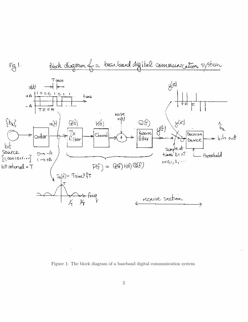
Figure 1: The block diagram of a baseband digital communication system

2

transmitter. In practice, we will see later that the cutoff frequency of the

Tx filter is placed approximately at the value 1/2T Hz., which corresponds

to half the main lobe width of the PSD Sa(f). We will discuss in detail later

the impact this filtering has on the shape of the pulse corresponding to a

single bit.

The block that follows the TX filter in Fig. 1 is the channel, whose

frequency response is denoted H(f). The channel is the medium over which

the digital signal is transmitted; e.g., the telephone wire, a fibre optic cable,

the airwaves, a coaxial cable, etc. In the case of a telephone wire for example,

the frequency response of the channel rolls off at a rate proportional to 1/f .

In most other cases, the frequency response of the channel is flat, except for

the case of the airwaves, when multipath is present. It can then be quite

distorted as we saw in the tutorial.

The effect of thermal and other noise sources is to add a noise process to

the receiver input, as shown in Fig. 1. Even though the noise has a very low

power level, it can nevertheless significantly impact the performance of the

digital transmission system. This is because the signal level is comparable to

that of the noise in a typical receiver system. Since the noise is a Gaussian

process, there is a finite probability that the noise in any bit interval is large

enough that it could cause a transmitted bit to appear on the wrong side

of the threshold in the decision device. The receiver will then detect the

wrong value for that bit, resulting in a bit error. We wish to minimize the

probability of occurrence of bit errors.

The next block in the transmission system of Fig. 1 is the receiver

(Rx) filter. This, like the Tx filter, also has a cutoff of approximately 1/2T

3

Hz. The purpose of this filter is to reduce the noise power present at the

decision device of the receiver, thereby reducing the probability of a bit error

and improving performance. Recall that the power (variance) of a random

process is the area under the PSD function. Further recall that the power

spectral density Sy(f) of the output of a filter with frequency response Q(f)

(as in Fig. 1) is given by

Sy(f) = |Q(f)|2Sin(f), (1)

where Sin(f) is the PSD of the input process. In this case, since the noise

is white, Sin(f) = No/2, as discussed in class. Since Q(f) is a low–pass

function, the area under Sy(f) is much less than that under Sin(f), with

the result that the output noise level is significantly lower than the input

noise level. This will have a major impact on reducing bit errors.

After the receiver filter, the signal is sampled at the rate of 1/T samples

per second. The samples are then fed to a decision device, which is essentially

a 1-bit analogue–to–digital convertor. If y(nT ) > K, where K is a threshold

value, then the corresponding output bit b̂(nT ) = 1; otherwise b̂(nT ) = 0.

The threshold value K is typically set to zero.

2 The Pulse Shape and Inter-symbol Interference

(ISI)

As we saw earlier, the rectangular pulse shape a(t) shown in Fig. 1 at the

transmitter corresponding to a single bit is rectangular. This corresponds

to a PSD of the form sinc2, which has an infinite bandwidth. The transmit

4

0 1 2 3 4 5 6 7 8 9−0.4

−0.2

0

0.2

0.4

0.6

0.8

1Pulse shape of a single bit; alpha=0.2

time in bit intervals

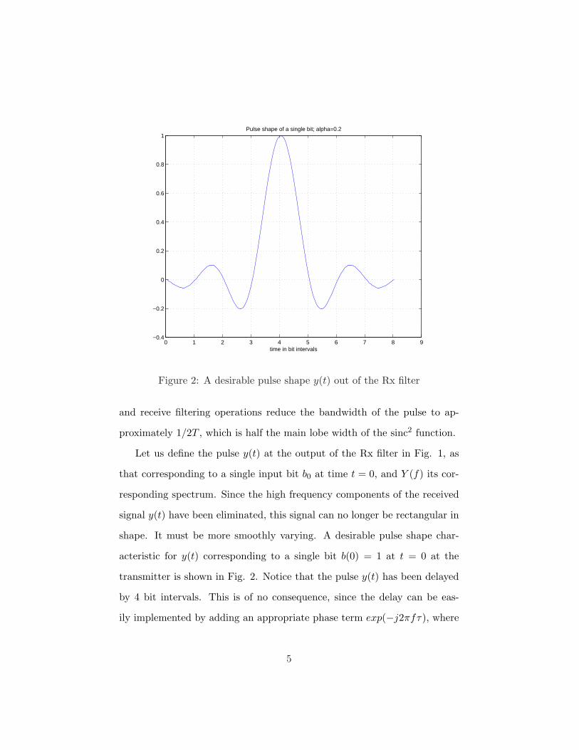
Figure 2: A desirable pulse shape y(t) out of the Rx filter

and receive filtering operations reduce the bandwidth of the pulse to ap-

proximately 1/2T , which is half the main lobe width of the sinc2 function.

Let us define the pulse y(t) at the output of the Rx filter in Fig. 1, as

that corresponding to a single input bit b0 at time t = 0, and Y (f) its cor-

responding spectrum. Since the high frequency components of the received

signal y(t) have been eliminated, this signal can no longer be rectangular in

shape. It must be more smoothly varying. A desirable pulse shape char-

acteristic for y(t) corresponding to a single bit b(0) = 1 at t = 0 at the

transmitter is shown in Fig. 2. Notice that the pulse y(t) has been delayed

by 4 bit intervals. This is of no consequence, since the delay can be eas-

ily implemented by adding an appropriate phase term exp(−j2πfτ), where

5

0 2 4 6 8 10 12 14 16 18−1

−0.8

−0.6

−0.4

−0.2

0

0.2

0.4

0.6

0.8

1ideal multiple pulses

time in bit intervals

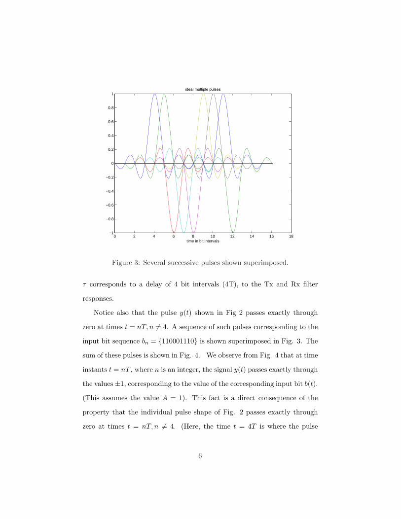
Figure 3: Several successive pulses shown superimposed.

τ corresponds to a delay of 4 bit intervals (4T), to the Tx and Rx filter

responses.

Notice also that the pulse y(t) shown in Fig 2 passes exactly through

zero at times t = nT, n 6= 4. A sequence of such pulses corresponding to the

input bit sequence bn = {110001110} is shown superimposed in Fig. 3. The

sum of these pulses is shown in Fig. 4. We observe from Fig. 4 that at time

instants t = nT , where n is an integer, the signal y(t) passes exactly through

the values ±1, corresponding to the value of the corresponding input bit b(t).

(This assumes the value A = 1). This fact is a direct consequence of the

property that the individual pulse shape of Fig. 2 passes exactly through

zero at times t = nT, n 6= 4. (Here, the time t = 4T is where the pulse

6

0 2 4 6 8 10 12 14 16 18−1.5

−1

−0.5

0

0.5

1

1.5sum of ideal pulses

Figure 4: The sum y(t) of the individual pulses of Fig. 3.

is maximum in absolute value, and is referred to as the sampling instant).

Our property can then be restated to say that the pulse passes through zero

at all multiples of the bit interval T , except for the sampling instant.

This property of the individual pulse is the key to successful digital

transmission. Suppose the pulse is distorted and this property does not hold.

Then the individual pulse does not pass through zero at the appropriate

instants, with the result that y(t) does not pass exactly through ±1 at

multiples of the bit interval. If the distortion is significant, and if the bit

values are such that the distortions all add up with the same polarity which

is opposite to that of the polarity of the pulse at the sampling instant,

then the distortions can add together so that y(t) is significantly reduced in

absolute value from the ideal levels of ±A. The result is that a lower level

7

noise can cause a bit error and the performance of the system degrades.

This form of distortion, i.e., when the pulse overlaps onto adjacent bit

intervals, is referred to as inter–symbol interference, or ISI. It is the cause

of significant degradation in digital transmission systems.

3 The Raised Cosine Pulse

We introduce this topic by first reviewing the theory on sampling of signals

in the time domain. Refer to Fig. 5. Recall that if a signal g(t) À G(f)

is sampled in the time domain at the rate of fs = 1/T samples per second,

then its spectrum becomes periodic with period fs Hz. The signal g(t) can

be recovered from its samples provided fo < fs/2, where fo is the highest

frequency component of G(f).

For zero ISI, the sampled signal y(nT ) out of the sampler must be a

finite value at a time t = noT where no corresponds to the sampling instant,

and zero for all other values of nT . This y(t) must be a discrete–time δ–

function; i.e., y(nT ) = δ(n− no). The corresponding periodically–repeating

spectrum must therefore be a constant in magnitude. It is sufficient for this

characteristic to be achieved if the spectrum Y (f) of y(t) before the sampler

is a rectangular function of width fs/2 = 1/2T , as shown in Fig. 6. The

edges of this rectangular function butt against each other after sampling and

the periodic version thus becomes a constant over all frequencies, as desired.

The corresponding y(t) before the sampler is therefore the Fourier trans-

form of a rectangle function, i.e., a sinc. Specifically, y(t) =√

Esinc(t/T +

8

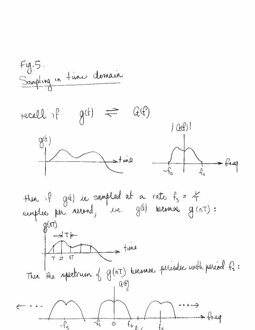
Figure 5: A review of samplingin the time domain.

9

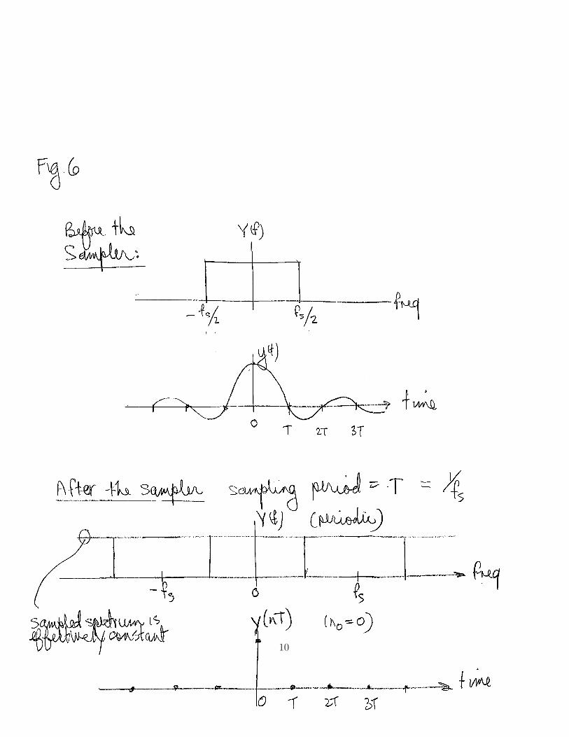
Figure 6: Sampling the sinc function.

10

to), where E is the energy of the pulse and to is the delay corresponding

to the sampling instant. This function has the desired property that it

goes through zero at multiples of the bit interval that are not equal to the

sampling instant.

If the system as we describe it is to work properly, then the spectrum

Y (f) must be a rectangular (ideal) low–pass function. As we know, this

function is impossible to implement exactly and can only be approximated.

However, a more serious difficulty associated with using the rectangular

frequency response Y (f) is that the corresponding sinc–function y(t) is very

sensitive to timing errors at the sampling instants. The sampling instants

are derived using a phase–locked loop and are never exactly error free. Let

the actual sampling instants te be defined as te = nT + ε, where ε represents

a timing error. It is clear that this timing error will introduce ISI because

y(t) is zero at the bit intervals only when ε = 0. The difficulty with the sinc

pulse is that of all the pulse shapes which result in zero ISI, it is the one

that is most sensitive to timing errors.

We can achieve a much lower sensitivity to timing errors by considering a

family of pulse shapes known as the raised cosine waveform. This reduction

in sensitivity is achieved at the expense of increased bandwidth. The trade-

off between low sensitivity on the one hand and increased bandwidth on

the other is controlled by a parameter α, where 0 ≤ α ≤ 1. Examples of

the raised cosine frequency response Y (f) corresponding to various values

of α are shown in Fig 7. Note that α = 0 is equivalent to the rectangular

frequency function. The corresponding pulse shapes y(t) are shown in Fig.

8. Note that these pulses all have the desired property of passing through

11

zero at t = nT , except for the sampling instant (which in the figure is at

zero).

The functions Y (f) in Fig. 7 for various values of α consist of a fitted

1/2-period of a cosine function between the normalized frequency values

|1/2−α/2| < |f | < |1/2+α/2|. When the raised cosine pulse is sampled with

a sampling period of T seconds, the raised cosine frequency response becomes

periodic and overlaps about the normalized frequency f = 1/2. Because of

the symmetry properties of the frequency response, the overlapped versions

of these responses add to give the normalized value of one, for all values

of α and all values of frequency, as shown in Fig. 9. Thus, the sampled

spectrum is still a constant, and the sampled pulse is still a discrete δ-

function, as desired. Note that as α increases towards one, the time domain

pulses decay more quickly, making the system less sensitive to ISI. However,

as α increases, the cost of the reduced ISI is that the required transmission

bandwidth also increases. Since bandwidth is very expensive, large values

of α have a cost. Formulas for the raised cosine spectrum Y (f) and the

corresponding inverse Fourier transform y(t) as a function of α are given in

the text, p. 238 2nd ed.

Note that the raised-cosine characteristic is achieved by designing the

combined frequency responses P (f) = G(f)H(f)Q(f) to be equal to the

raised cosine spectrum. This task is indeed possible if the frequency response

of the channel is known and fixed. However, in certain situations, e.g., with

wireless transmission in the presence of multipath, (as we discussed in the

tutorial), the frequency response of the channel can vary significantly with

time, thus destroying the desired raised-cosine characteristic. Maintaining

12

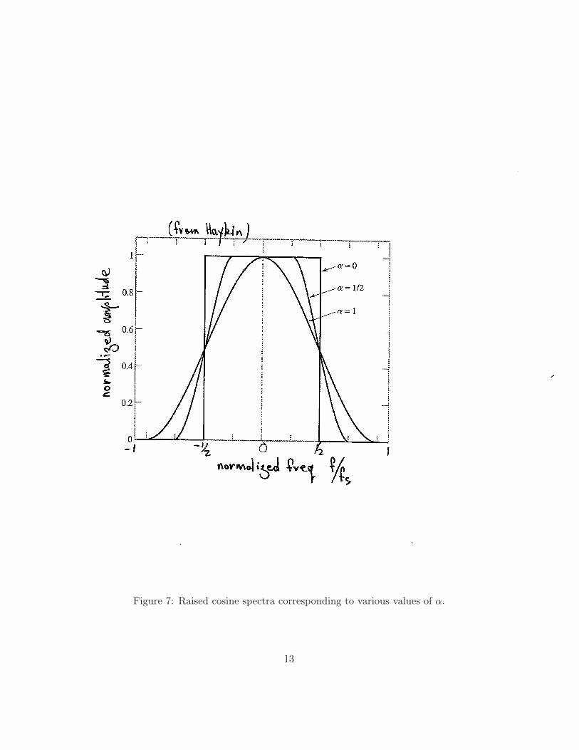
Figure 7: Raised cosine spectra corresponding to various values of α.

13

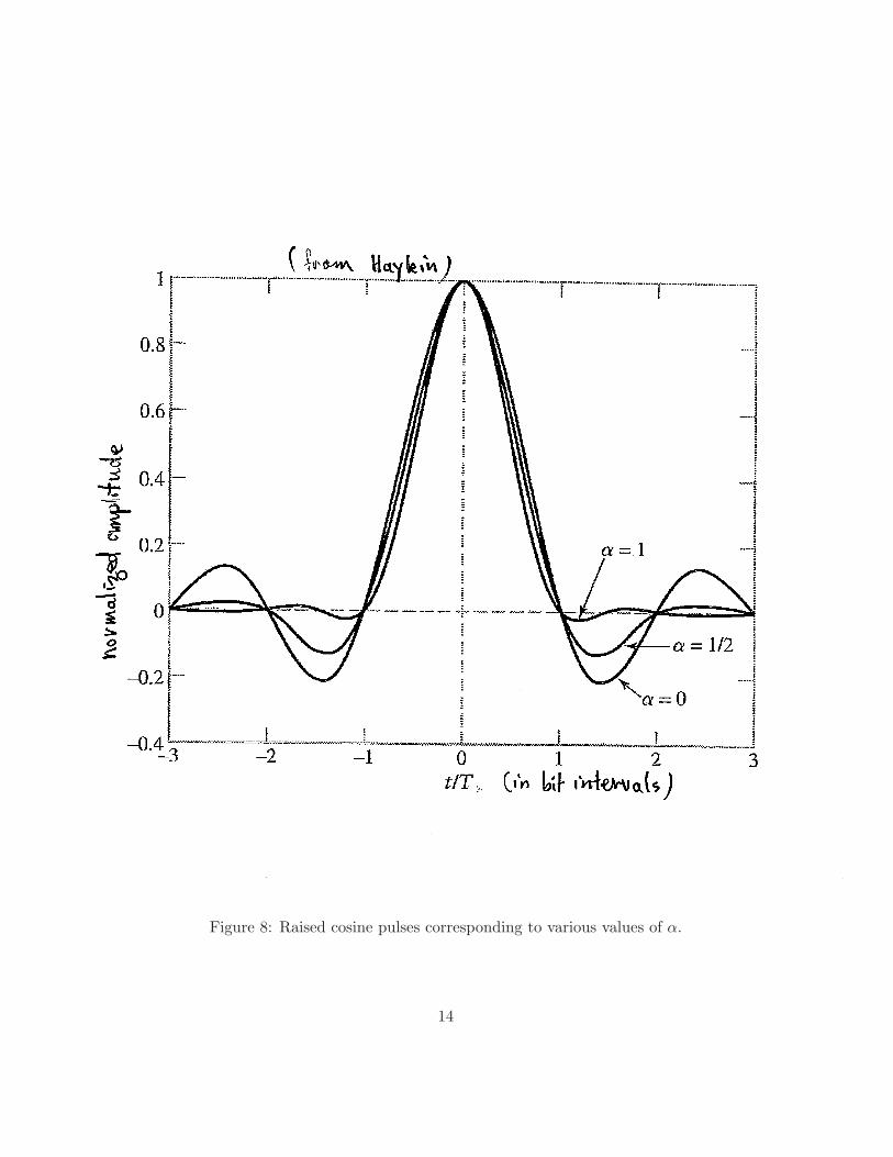
Figure 8: Raised cosine pulses corresponding to various values of α.

14

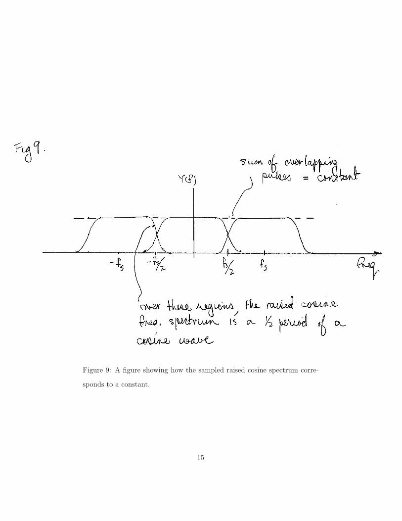
Figure 9: A figure showing how the sampled raised cosine spectrum corre-

sponds to a constant.

15

the desired spectrum of the overall communications system in the case where

the channel varies with time is referred to as equalization. This is a very

interesting and important topic and is discussed to a certain degree in the

4th year elective communications course, EE4TK4.

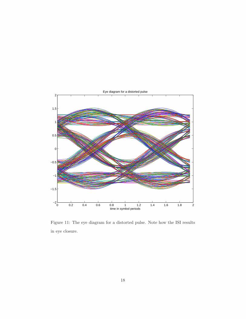
4 The eye diagram

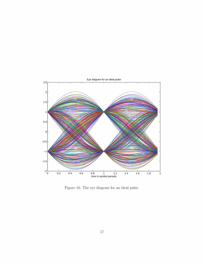
Consider the equivalent of the signal in Fig. 4 corresponding to a long

sequence of bits. Suppose that we were to extract segments of this signal of

length equal to two symbol periods (2T ), and superimpose them over top

of each other on a single graph. This graph is called the eye diagram, due

to its similarity with the human eye. If the number of segments is long

enough, this graph would show the trajectories of the pulse as it makes

its transitions over all possible bit values. If the pulse shape is ideal with

no ISI, then all such segments will pass exactly through the values ±A at

the sampling instant and the eye diagram consists of only two points at

the sampling instant. If the pulse shape does contain some ISI, then the

segments will be dispersed about the values ±A. The eye diagram then

partially “closes”, as shown in Figs. 10 and Fig. 11. The eye diagram is

an excellent way to assess the impact of ISI, and clearly shows how ISI can

reduce the immunity of the system to noise.

16

0 0.2 0.4 0.6 0.8 1 1.2 1.4 1.6 1.8 2−2

−1.5

−1

−0.5

0

0.5

1

1.5

2

2.5Eye diagram for an ideal pulse

time in symbol periods

Figure 10: The eye diagram for an ideal pulse.

17

0 0.2 0.4 0.6 0.8 1 1.2 1.4 1.6 1.8 2−2

−1.5

−1

−0.5

0

0.5

1

1.5

2Eye diagram for a distorted pulse

time in symbol periods

Figure 11: The eye diagram for a distorted pulse. Note how the ISI results

in eye closure.

18