Embed Size (px)
Citation preview
Diagnostic and Prognostic InferenceCutting Scores, Base Rates, and Decision Theory
Base Rates and Bayes’ TheoremSlides to accompany Grove’s handout
Scott Vrieze
March 8, 2016
Scott Vrieze Base Rates and Bayes’ Theorem
Diagnostic and Prognostic InferenceCutting Scores, Base Rates, and Decision Theory
Table of contents
1 Diagnostic and Prognostic Inference
2 Cutting Scores, Base Rates, and Decision Theory
Scott Vrieze Base Rates and Bayes’ Theorem
Diagnostic and Prognostic InferenceCutting Scores, Base Rates, and Decision Theory
Example inferences
Does this patient have Alzheimer’s disease, schizophrenia,depression, etc.?
What is the patient’s cognitive ability?
How amenable is this patient to talk therapy?
Was this individual abused as a child?
Scott Vrieze Base Rates and Bayes’ Theorem
Diagnostic and Prognostic InferenceCutting Scores, Base Rates, and Decision Theory
Pieces of information
Symptoms Self-report measures obtained via interview,whether structured or not
Behavioral observations and other signs Signs areobservable characteristics, in contrast to symptoms
Life history facts
Psychological test results such as scores or unscored data
Physiological measures
Others?
Scott Vrieze Base Rates and Bayes’ Theorem
Diagnostic and Prognostic InferenceCutting Scores, Base Rates, and Decision Theory
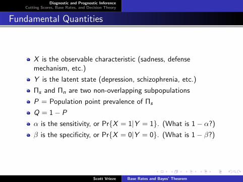
Fundamental Quantities
X is the observable characteristic (sadness, defensemechanism, etc.)
Y is the latent state (depression, schizophrenia, etc.)
Πs and Πn are two non-overlapping subpopulations
P = Population point prevalence of Πs
Q = 1− P
α is the sensitivity, or PrX = 1|Y = 1. (What is 1− α?)
β is the specificity, or PrX = 0|Y = 0. (What is 1− β?)
Scott Vrieze Base Rates and Bayes’ Theorem
Diagnostic and Prognostic InferenceCutting Scores, Base Rates, and Decision Theory
Bayes’ Theorem
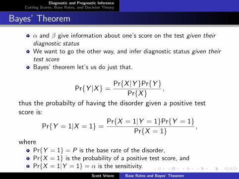
α and β give information about one’s score on the test given theirdiagnostic statusWe want to go the other way, and infer diagnostic status given theirtest scoreBayes’ theorem let’s us do just that.
PrY |X =PrX |Y PrY
PrX,
thus the probabilty of having the disorder given a positive testscore is:
PrY = 1|X = 1 =PrX = 1|Y = 1PrY = 1
PrX = 1,
wherePrY = 1 = P is the base rate of the disorder,PrX = 1 is the probability of a positive test score, andPrX = 1|Y = 1 = α is the sensitivity.
Scott Vrieze Base Rates and Bayes’ Theorem

Diagnostic and Prognostic InferenceCutting Scores, Base Rates, and Decision Theory
Derived Quantities: PPV & NPV
Positive predictive value: Probability one is called a case, givenone scores positive on the test.
PPV = PrY = 1|X = 1
=PrX = 1|Y = 1PrY = 1
PrX = 1(1)
=Pα
Pα + Q(1− β)
Negative predictive value: Probability one is called a noncasegiven one scores negative on the test.
NPV = PrY = 0|X = 0
=PrX = 0|Y = 0PrY = 0
PrX = 0(2)
=Qβ
P(1− α) + Qβ
Scott Vrieze Base Rates and Bayes’ Theorem
Diagnostic and Prognostic InferenceCutting Scores, Base Rates, and Decision Theory
Derived Quantities: Hit Rate (aka Efficiency)
Hit Rate: Proportion of individuals correctly classified.
HR = Pα + Qβ
Scott Vrieze Base Rates and Bayes’ Theorem

Diagnostic and Prognostic InferenceCutting Scores, Base Rates, and Decision Theory
Likelihood and Likelihood Ratio
Probability mass function:
g(x ; n, p) =
(n
x
)px(1− p)n−x
Probability density function:
g(x ;µ, σ2) =1
σ√
2πe−
(x−µ)2
2σ2
These are probability functions when we consider theparameters fixed and the observed scores x random.
They are likelihood functions when the observed scores x arefixed (e.g., we collected data) and the parameters are random.
Scott Vrieze Base Rates and Bayes’ Theorem
Diagnostic and Prognostic InferenceCutting Scores, Base Rates, and Decision Theory
Likelihood and Likelihood Ratio
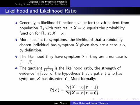
Generally, a likelihood function’s value for the ith patient frompopulation Πs with test result X = xi equals the probabilityfunction for Πs at X = xi .
More specific to symptoms, the likelihood that a randomlychosen individual has symptom X given they are a case is α,by definition.
The likelihood they have symptom X if they are a noncase is(1− β).
The quotient α(1−β) is the likelihood ratio, the strength of
evidence in favor of the hypothesis that a patient who hassymptom X has disorder Y . More formally:
Ω(xi ) =PrX = xi |Y = 1PrX = xi |Y = 0
Scott Vrieze Base Rates and Bayes’ Theorem

Diagnostic and Prognostic InferenceCutting Scores, Base Rates, and Decision Theory
Likelihood and Likelihood Ratio
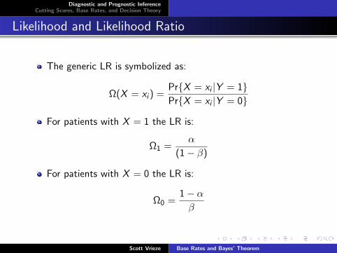
The generic LR is symbolized as:
Ω(X = xi ) =PrX = xi |Y = 1PrX = xi |Y = 0
For patients with X = 1 the LR is:
Ω1 =α
(1− β)
For patients with X = 0 the LR is:
Ω0 =1− αβ
Scott Vrieze Base Rates and Bayes’ Theorem
Diagnostic and Prognostic InferenceCutting Scores, Base Rates, and Decision Theory
Likelihood and Likelihood Ratio
The generic LR is symbolized as:
Ω(X = xi ) =PrX = xi |Y = 1PrX = xi |Y = 0
For patients with X = 1 the LR is:
Ω1 =α
(1− β)
For patients with X = 0 the LR is:
Ω0 =1− αβ
Scott Vrieze Base Rates and Bayes’ Theorem
Diagnostic and Prognostic InferenceCutting Scores, Base Rates, and Decision Theory
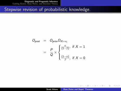
Stepwise revision of probabilistic knowledge.
Opost = OpriorΩX=xi
=P
Q×
α
(1−β) , if X = 1
(1−α)β , if X = 0
Scott Vrieze Base Rates and Bayes’ Theorem
Diagnostic and Prognostic InferenceCutting Scores, Base Rates, and Decision Theory
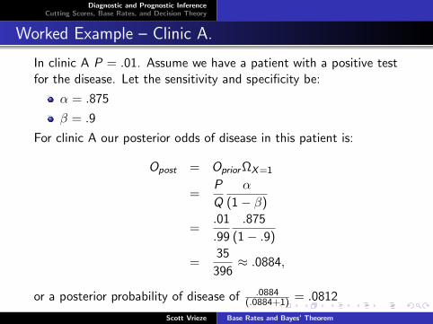
Worked Example – Clinic A.
In clinic A P = .01. Assume we have a patient with a positive testfor the disease. Let the sensitivity and specificity be:
α = .875
β = .9
For clinic A our posterior odds of disease in this patient is:
Opost = OpriorΩX=1
=P
Q
α
(1− β)
=.01
.99
.875
(1− .9)
=35
396≈ .0884,
or a posterior probability of disease of .0884(.0884+1) = .0812
Scott Vrieze Base Rates and Bayes’ Theorem
Diagnostic and Prognostic InferenceCutting Scores, Base Rates, and Decision Theory
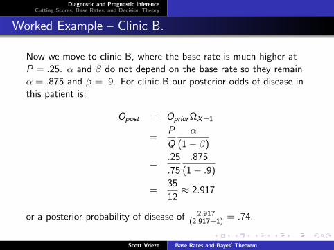
Worked Example – Clinic B.
Now we move to clinic B, where the base rate is much higher atP = .25. α and β do not depend on the base rate so they remainα = .875 and β = .9. For clinic B our posterior odds of disease inthis patient is:
Opost = OpriorΩX=1
=P
Q
α
(1− β)
=.25
.75
.875
(1− .9)
=35
12≈ 2.917
or a posterior probability of disease of 2.917(2.917+1) = .74.
Scott Vrieze Base Rates and Bayes’ Theorem
Diagnostic and Prognostic InferenceCutting Scores, Base Rates, and Decision Theory
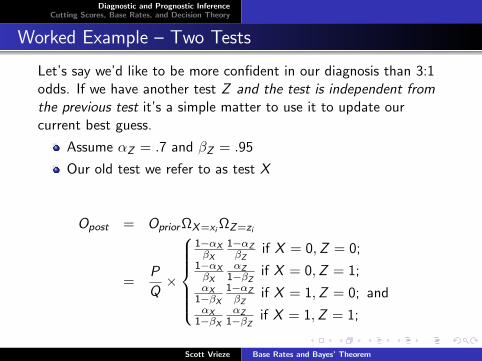
Worked Example – Two Tests
Let’s say we’d like to be more confident in our diagnosis than 3:1odds. If we have another test Z and the test is independent fromthe previous test it’s a simple matter to use it to update ourcurrent best guess.
Assume αZ = .7 and βZ = .95
Our old test we refer to as test X
Opost = OpriorΩX=xi ΩZ=zi
=P
Q×
1−αXβX
1−αZβZ
if X = 0,Z = 0;1−αXβX
αZ1−βZ if X = 0,Z = 1;
αX1−βX
1−αZβZ
if X = 1,Z = 0; andαX
1−βXαZ
1−βZ if X = 1,Z = 1;
Scott Vrieze Base Rates and Bayes’ Theorem

Diagnostic and Prognostic InferenceCutting Scores, Base Rates, and Decision Theory
Two independent Tests
Let’s say we’d like to be more confident in our diagnosis than 3:1odds. If we have another test Z and the test is independent fromthe previous test it’s a simple matter to use it to update ourcurrent best guess.
Assume αZ = .7 and βZ = .95
Our old test we refer to as test X
A positive test result on tests X and Z in clinic B results in:
Opost = OpriorΩX=xi ΩZ=zi
=.25
.75
.875
1− .9.7
1− .95= 40.833,
a posterior probability of 40.8331+40.833 = .98.
Scott Vrieze Base Rates and Bayes’ Theorem
Diagnostic and Prognostic InferenceCutting Scores, Base Rates, and Decision Theory
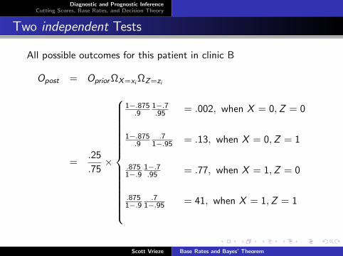
Two independent Tests
All possible outcomes for this patient in clinic B
Opost = OpriorΩX=xi ΩZ=zi
=.25
.75×
1−.875.9
1−.7.95 = .002, when X = 0,Z = 0
1−.875.9
.71−.95 = .13, when X = 0,Z = 1
.8751−.9
1−.7.95 = .77, when X = 1,Z = 0
.8751−.9
.71−.95 = 41, when X = 1,Z = 1
Scott Vrieze Base Rates and Bayes’ Theorem
Diagnostic and Prognostic InferenceCutting Scores, Base Rates, and Decision Theory
Total Relevant Evidence
More ‘information’ is not necessarily better, especially whenyou’re a human judge.
Independent and valid evidence (tests) is ideal. This is alsorare.
Combining information across multiple correlated tests istricky and depends on the strength of correlation, which couldbe different in the cases versus controls.
This issue will come up later when we discuss incrementalvalidity.
Scott Vrieze Base Rates and Bayes’ Theorem
Diagnostic and Prognostic InferenceCutting Scores, Base Rates, and Decision Theory
Cutting Scores and (Quasi-) Continuous Tests
Show program. Note that cutting score affects sensitivity &specificity and thereby hit rate. Optimal cutting score depends onthe test score distributions (separation, size, shape).
Scott Vrieze Base Rates and Bayes’ Theorem
Diagnostic and Prognostic InferenceCutting Scores, Base Rates, and Decision Theory
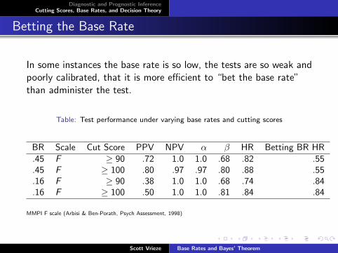
Betting the Base Rate
In some instances the base rate is so low, the tests are so weak andpoorly calibrated, that it is more efficient to “bet the base rate”than administer the test.
Table: Test performance under varying base rates and cutting scores
BR Scale Cut Score PPV NPV α β HR Betting BR HR.45 F ≥ 90 .72 1.0 1.0 .68 .82 .55.45 F ≥ 100 .80 .97 .97 .80 .88 .55.16 F ≥ 90 .38 1.0 1.0 .68 .74 .84.16 F ≥ 100 .50 1.0 1.0 .81 .84 .84
MMPI F scale (Arbisi & Ben-Porath, Psych Assessment, 1998)
Scott Vrieze Base Rates and Bayes’ Theorem
Diagnostic and Prognostic InferenceCutting Scores, Base Rates, and Decision Theory
Simple Decision-Theoretic Analysis
So far our goal has been to maximize correct classifications ofdisorder. If Opost > 1, diagnose disease. If Opost < 1 do not.
We have ignored the costs of making different decisions,which may affect how cautious or aggressive we are in makingdiagnoses.
Scott Vrieze Base Rates and Bayes’ Theorem
Diagnostic and Prognostic InferenceCutting Scores, Base Rates, and Decision Theory
Simple Decision-Theoretic Analysis: Classic Example
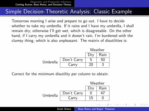
Tomorrow morning I arise and prepare to go out. I have to decidewhether to take my umbrella. If it rains and I have my umbrella, I shallremain dry; otherwise I’ll get wet, which is disagreeable. On the otherhand, if I carry my umbrella and it doesn’t rain, I’m burdened with theclumsy thing, which is also unpleasant. The matrix of disutilities is:
WeatherDry Rain
UmbrellaDon’t Carry 5 50
Carry 20 3
Correct for the minimum disutility per column to obtain:
WeatherDry Rain
UmbrellaDon’t Carry 0 47
Carry 15 0
Scott Vrieze Base Rates and Bayes’ Theorem
Diagnostic and Prognostic InferenceCutting Scores, Base Rates, and Decision Theory
Simple Decision-Theoretic Analysis: Incorporating BaseRates
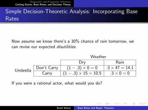
Now assume we know there’s a 30% chance of rain tomorrow, wecan revise our expected disutilities:
WeatherDry Rain
UmbrellaDon’t Carry (1− .3)× 0 = 0 .3× 47 = 14.1
Carry (1− .3)× 15 = 10.5 .3× 0 = 0
If you were a rational actor, what would you do?
Scott Vrieze Base Rates and Bayes’ Theorem
Diagnostic and Prognostic InferenceCutting Scores, Base Rates, and Decision Theory
Complicated Decision-Theoretic Analysis
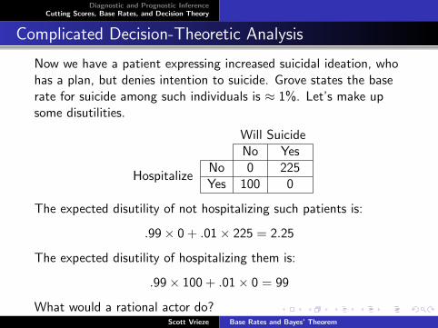
Now we have a patient expressing increased suicidal ideation, whohas a plan, but denies intention to suicide. Grove states the baserate for suicide among such individuals is ≈ 1%. Let’s make upsome disutilities.
Will SuicideNo Yes
HospitalizeNo 0 225Yes 100 0
The expected disutility of not hospitalizing such patients is:
.99× 0 + .01× 225 = 2.25
The expected disutility of hospitalizing them is:
.99× 100 + .01× 0 = 99
What would a rational actor do?Scott Vrieze Base Rates and Bayes’ Theorem
Diagnostic and Prognostic InferenceCutting Scores, Base Rates, and Decision Theory
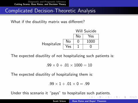
Complicated Decision-Theoretic Analysis
What if the disutility matrix was different?
Will SuicideNo Yes
HospitalizeNo 0 1000Yes 1 0
The expected disutility of not hospitalizing such patients is:
.99× 0 + .01× 1000 = 10
The expected disutility of hospitalizing them is:
.99× 1 + .01× 0 = .99
Under this scenario it “pays” to hospitalize such patients.
Scott Vrieze Base Rates and Bayes’ Theorem
Diagnostic and Prognostic InferenceCutting Scores, Base Rates, and Decision Theory
Does this seem appealing?
How difficult is it to do this?
Who are the stakeholders, how do you measuretheir disutilities, how do you weight them?
Is difficulty a reason to ignore these issues?
Scott Vrieze Base Rates and Bayes’ Theorem