Bargaining for the American Dream · Bargaining for the American Dream ... Bargaining for the American Dream Introduction and summary ... study on interest groups and political influence

WWW.AMERICANPROGRESS.ORG

AP/M

ARY A

LTAFFER

Bargaining for the American DreamWhat Unions do for Mobility

By Richard Freeman, Eunice Han, David Madland, and Brendan V. Duke September 2015

Bargaining for the American DreamWhat Unions do for Mobility

By Richard Freeman, Eunice Han, David Madland, and Brendan V. Duke September 2015

1 Introduction and summary

4 Unions and intergenerational mobility by area

10 Mobility in union and nonunion households

14 Unions and stagnant intergenerational mobility

16 Conclusion

17 Appendix A: Area-level data

20 Appendix B: Area-level analysis

24 Appendix C: Individual household data and analysis

31 Endnotes

Contents

1 Center for American Progress | Bargaining for the American Dream

Introduction and summary

One of the central challenges facing the United States on which both progressives and conservatives can agree is the need to increase economic mobility. Upward mobility and opportunity are the definition of the American dream. But today, the nation has less mobility and fewer opportunities when compared to other advanced economies. A U.S. child born in the bottom 20 percent of the income distribution, for example, has a 7.5 percent probability of reaching the top 20 percent as an adult, compared to 11.7 percent in Denmark and 13.4 percent in Canada.1 Increasing mobility, however, requires understanding why it is low.

Research by economists Raj Chetty of Stanford University, Nathaniel Hendren of Harvard University and Patrick Kline and Emmanuel Saez of the University of California, Berkeley, shows that some regions of the United States have levels of mobility—that is to say, the ability to improve upon the situation of one’s birth—similar to Denmark and Canada. However, that same research reveals that other U.S. areas have mobility levels that are lower than any other advanced economy for which data are available. The research of Chetty and his fellow authors also show that five factors have the strongest geographical relationship—positive or negative—with mobility: single motherhood rates, income inequality, high school dropout rates, social capital, and segregation.2

This report examines the relationship between mobility and another variable that Chetty and his co-authors did not consider: union membership. The analysis in this report begins on the area level using the same methodological approach as Chetty and his co-authors for their five factors. But the analysis then goes beyond this area-level analysis, using another dataset that matches parents with children that allows for the comparison of outcomes for children who grew up in otherwise similar union and nonunion households. This individual-level analysis is more appropriate than the area-level analysis for examining whether parents’ union membership actually influences mobility.


* All reference to “we,” “us,” and “our” refer to the authors of this report.

Based on the research for this report, it is clear that there is a strong relationship between union membership and intergenerational mobility. More specifically:

• Areas with higher union membership demonstrate more mobility for low-

income children. Using Chetty and others’ data, we* find that low-income children rise higher in the income rankings when they grow up in areas with high-union membership. A 10 percentage point increase in a geographic area’s union membership is associated with low-income children ranking 1.3 per-centile points higher in the national income distribution. This relationship between unions and the mobility of low-income children is at least as strong as the relationship between mobility and high school dropout rates—a factor that is generally recognized as one of the most important correlates of eco-nomic mobility. Indeed, union density is one of the strongest predictors of an area’s mobility. Furthermore, unions remain a significant predictor of economic mobility even after one controls for several variables including race, types of industries, inequality, and more.

• Areas with higher union membership have more mobility as measured by

all children’s incomes. We also measure the geographic relationship between union membership and another measure of mobility: the income of all children who grew up in an area after controlling for their parents’ incomes. According to our findings, a 10 percentage point increase in union density is associated with a 4.5 percent increase in the income of an area’s children. Here again, union density compares quite favorable with other common predictors of an area’s mobility. In addition, the relationship between unions and the mobility of all children remains strong after adopting several additional controls.

• Children who grow up in union households have better outcomes. Using a differ-ent dataset, we match parents and children to compare the outcomes of children who grew up in otherwise similar union and nonunion households. The findings show that children growing up in union households tend to have better outcomes than children who grew up in nonunion households, especially when the parents are low skilled. For example, children of non-college-educated fathers earn 28 percent more if their father was in a labor union. This analysis helps provide evi-dence suggesting a link between unions and economic mobility.

These findings are new and illustrate a previously ignored factor that could be essential for promoting economic mobility. However, they are not surprising, par-ticularly given the extensive research that has been done on unions and middle-


class incomes. Previous research by the CAP Action Fund has found a strong geographical relationship between union membership and intragenerational mobility—the relationship between someone’s earnings when they are 35 to 39 years old and when they are 45 to 49 years old.3 Our findings also coincide with the findings of several studies showing that falling union membership has been a key driver in the rise of income inequality.4 Most recently, Bruce Western and Jake Rosenfeld of Harvard and the Washington University at St. Louis, respectively, found that the decline of labor unions explains up to one-third of the increase in male wage inequality between 1973 and 2007.5

There are strong reasons to believe that unions may increase opportunity. First, there are the direct effects that a parent’s union membership may have on their children. Union workers make more money than comparable nonunion work-ers—what economists call the union premium—and when parents make more money, their children tend to make more money—which economists refer to as the intergenerational earnings elasticity. In theory, unionized parents should pass on a portion of the union premium to their children. There may be other chan-nels through which children whose parents were in a union have better outcomes than other children: union jobs may be more stable and predictable, which could produce a more stable living environment for children, and union jobs are more likely to provide family health insurance.

But there are also a series of other ways that unions could boost intergenerational mobility for nonunion workers. It has been shown that unions push up wages for nonunion workers, for example, and these wage gains for nonunion members could be passed on to their children.6 Children who grow up in nonunion house-holds may also display more mobility in highly unionized areas, for example, because they may be able to join a union when they enter the labor market. Finally, unions generally advocate for policies that benefit all working people—such as minimum wage increases and increased expenditures on schools and public ser-vices—that may especially benefit low-income parents and their children. A recent study on interest groups and political influence found that most of the national groups that supported middle-class priorities were unions.7 Another study found that states with higher union density also have higher minimum wages.8

In short, there are many theoretical reasons to expect unions to go hand in hand with economic mobility, and this paper provides empirical evidence that this is indeed the case.


Unions and intergenerational mobility by area

In 2013, Chetty, Hendren, Kline, and Saez made headlines with their paper “Where is the Land of Opportunity? The Geography of Intergenerational Mobility in the United States.” Using federal tax records, they were able to estimate the relationship between parent and child incomes—intergenerational mobility—with more precision than previous datasets. Measuring the variation in mobility in areas—what they call commuting zones, or CZs—across the country, they found that some areas such as Pittsburgh, Pennsylvania, and Minneapolis, Minnesota, had much higher mobility than other areas such as Charlotte, North Carolina, and Atlanta, Georgia.

The main limitation of using tax records, however, is the lack of detailed individual demographic and socioeconomic data that would allow scholars to examine par-ents’ and children’s characteristics that have the closest associations with intergen-erational mobility. Instead, Chetty and his co-authors combined the geographical mobility estimates with rich demographic and social statistics on commuting zones from public data sources to examine the geographical correlation. They found that five factors had the strongest relationship with mobility across com-muting zones: the percent of children with single mothers, social capital, income inequality, high school dropout rates, and a measure of residential segregation—the percentage of workers with less than 15 minute commutes to their jobs.

Chetty and his co-authors rightly emphasize that the geographical correlations they find are not necessarily causal, but rather serve as “a set of stylized facts to guide the search for causal determinants and the development of new models of intergenerational mobility.”9 What our geographical analysis does establish is the stylized fact that regions with higher union membership exhibit higher intergener-ational mobility. Our analysis in the next section investigates this relationship more closely, using survey data to examine the relationship between individual parents’ union status and their children’s mobility while controlling for more factors.


Using two geographic measures of mobility, we follow the same approach as Chetty and his co-authors to examine their relationship with unions: We calcu-late the percent of workers in a commuting zone who are members of a union—referred to as union density—and measure its correlation with mobility across commuting zones. To see how we constructed the union variable and the com-muting zones, see Appendix A.

Mobility for low-income children

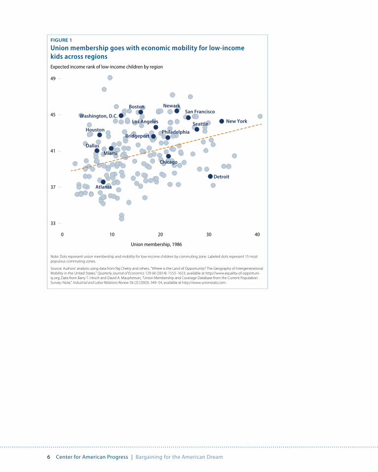
The main variable Chetty and his co-authors use to measure geographical mobil-ity is what they call absolute upward mobility—the expected rank in the national income distribution of a 29- to 32-year-old whose parents were in the 25th percentile of the national income distribution. We use the same variable in their analysis, but call it “mobility for low-income children” to avoid confusion with our other mobility measure.

In our sample’s average commuting zone, the average 29- to 32-year old whose parents were in the 25th percentile of the national income distribution ends up in the 40.7th percentile as an adult. We find a very strong correlation between unions and mobility across commuting zones: A 10 percentage point increase in the share of workers in a union is associated with a 1.3 percentile increase in children’s rank. As a point of comparison, the difference in mobility between San Francisco, California and Atlanta, Georgia—respectively, one of the most and one of the least mobile of the 25 largest CZs—is 7.1 percentile points.

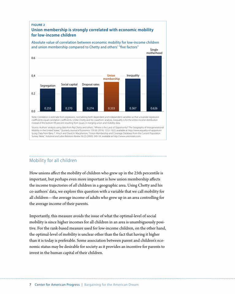
Figure 2 compares the size of the correlation between areas’ union membership rates with the five other factors Chetty and his co-authors identified as having the strongest correlation with mobility.10 The relationship between unionization and mobility is about the same as the relationship between residential segregation and high school dropout rates, two commonly cited drivers of mobility. Even when one controls for several variables—a commuting zone’s racial makeup, industry makeup, Chetty’s five factors, the number of children per family, the child pov-erty rate, the median house value, the progressivity of the tax code, and the share of families covered by a state’s Earned Income Tax Credit, or EITC—the share of workers in a union remains a significant correlate of mobility for low-income children. For details on the analysis, see Appendix B.


FIGURE 1

Union membership goes with economic mobility for low-income kids across regions

Note: Dots represent union membership and mobility for low-income children by commuting zone. Labeled dots represent 15 most populous commuting zones.

Source: Authors' analysis using data from Raj Chetty and others, "Where is the Land of Opportunity? The Geography of Intergenerational Mobility in the United States," Quarterly Journal of Economics 129 (4) (2014): 1553–1623, available at http://www.equality-of-opportuni-ty.org; Data from Barry T. Hirsch and David A. Macpherson, "Union Membership and Coverage Database from the Current Population Survey: Note," Industrial and Labor Relations Review 56 (2) (2003): 349–54, available at http://www.unionstats.com.

Expected income rank of low-income children by region

0 10 20 30 40

33

37

41

45

49

Union membership, 1986

Houston

Dallas

Atlanta

Miami

Boston

Washington, D.C.Los Angeles

Bridgeport

NewarkSan Francisco

Detroit

New YorkSeattle

Chicago

Philadelphia


Mobility for all children

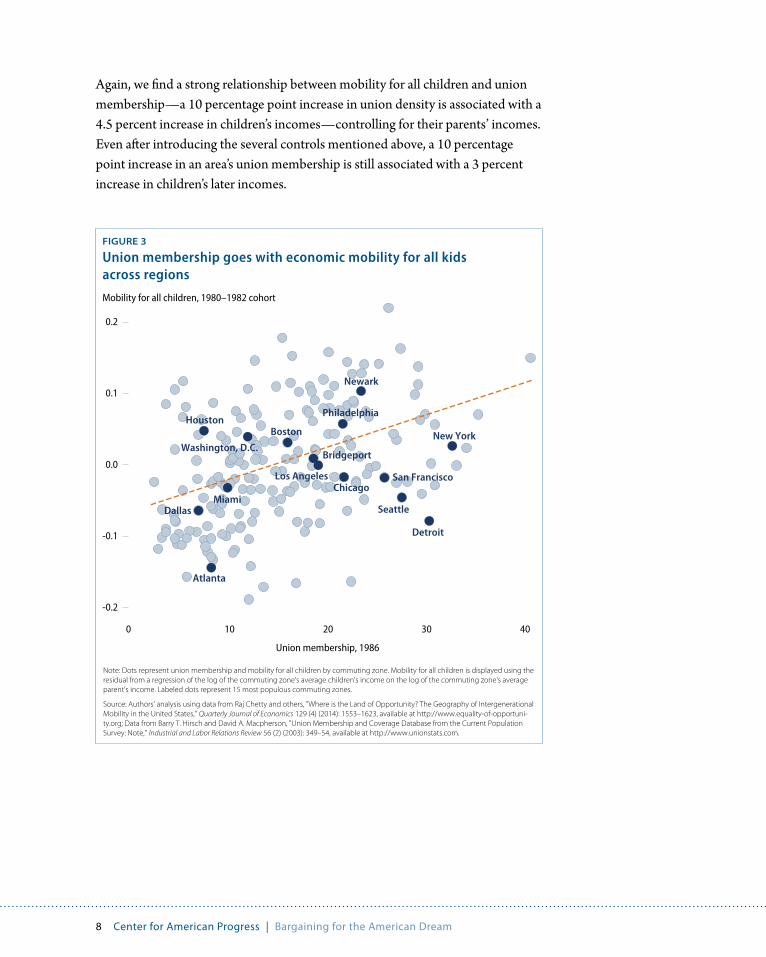
How unions affect the mobility of children who grew up in the 25th percentile is important, but perhaps even more important is how union membership affects the income trajectories of all children in a geographic area. Using Chetty and his co-authors’ data, we explore this question with a variable that we call mobility for all children—the average income of adults who grew up in an area controlling for the average income of their parents.

Importantly, this measure avoids the issue of what the optimal-level of social mobility is since higher incomes for all children in an area is unambiguously posi-tive. For the rank-based measure used for low-income children, on the other hand, the optimal-level of mobility is unclear other than the fact that having it higher than it is today is preferable. Some association between parent and children’s eco-nomic status may be desirable for society as it provides an incentive for parents to invest in the human capital of their children.

FIGURE 2

Union membership is strongly correlated with economic mobility for low-income children

Absolute value of correlation between economic mobility for low-income children and union membership compared to Chetty and others' "five factors"

Note: Correlation is estimate from regression, normalizing both dependent and independent variables so that univariate regression coe�cients equal correlation coe�cients. Unlike Chetty and his coauthors’ analysis, inequality is for the entire income distribution instead of the bottom 99 percent resulting from issues in merging union and mobility data.


0.0

0.2

0.4

0.6

Segregation Social capital Dropout rates

Single motherhood

Union membership

0.255 0.270 0.274 0.333 0.367 0.626

Inequality


Again, we find a strong relationship between mobility for all children and union membership—a 10 percentage point increase in union density is associated with a 4.5 percent increase in children’s incomes—controlling for their parents’ incomes. Even after introducing the several controls mentioned above, a 10 percentage point increase in an area’s union membership is still associated with a 3 percent increase in children’s later incomes.

FIGURE 3

Union membership goes with economic mobility for all kids across regions

Note: Dots represent union membership and mobility for all children by commuting zone. Mobility for all children is displayed using the residual from a regression of the log of the commuting zone's average children's income on the log of the commuting zone's average parent's income. Labeled dots represent 15 most populous commuting zones.


0 10 20 30 40

-0.2

-0.1

0.0

0.1

0.2

Union membership, 1986

Mobility for all children, 1980–1982 cohort

Houston

Dallas

Atlanta

Miami

Boston

Washington, D.C.

Los Angeles

Newark

San Francisco

Detroit

New York

Seattle

Chicago

Philadelphia

Bridgeport


Discussion

This analysis reveals that areas with higher union membership have higher mobil-ity not just for low- income children, but for all children. This relationship holds even after controlling for several other factors, some of which may serve as a chan-nel for how unions increase mobility. Our analysis, for example, controls for tax progressivity, which Chetty and his co-authors find has a positive correlation with mobility. Unions, of course, are possibly the most important advocates in states for progressive tax codes and that may be one of the key ways that unions increase mobility. By controlling for tax progressivity and other variables such as social capital that a region’s union membership likely influences, we have subjected the union-mobility relationship to a stringent test that it appears to have passed.

Nevertheless, Chetty and his co-authors caution that the correlations they find—such as the strongly negative relationship between single motherhood rates and mobility—should be interpreted as a set of correlations and stylized facts rather than a causal finding. The same caveat applies to our findings about the spatial relationship between unions and intergenerational mobility. What is clear, how-ever, is that mobility thrives in areas where unions thrive.

Note: Correlation is estimate from regression, normalizing both dependent and independent variables so that univariate regression coe�cients equal correlation coe�cients


FIGURE 4

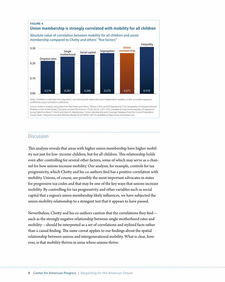
Union membership is strongly correlated with mobility for all children

Absolute value of correlation between mobility for all children and union membership compared to Chetty and others' "five factors"

0.00

0.10

0.20

0.30

Dropout rates

Single motherhood

Social capital SegregationUnion

membership

Inequality

0.219 0.247 0.260 0.270 0.271 0.310


Mobility in union and nonunion households

More confidence can be developed that there is a strong relationship between unions and upward mobility by using household-level data to compare the trajectories of children from union and similar nonunion households. Ideally, randomized controls could be performed or a natural experiment could be identi-fied where the assignment of union membership is random and mobility could be measured. Unfortunately, that is not plausible. Instead, we use survey data and control for several observable characteristics of the parents, including race, educa-tion, industry, occupation, age, work status, and urban status.

The Panel Study of Income Dynamics, or PSID, is the best dataset for this work because it not only tracks households, but when children from the original house-hold form their own household, it continues to collect information about them. Therefore, it is possible to combine the characteristics of 26- to 37-year olds in 2011 with the characteristics of their parents in 1985 and compare the trajectories of children whose parents were otherwise similar except for their union status. See Appendix C for more details.

Similar to the geographic analysis, we examine whether parents’ union status boosts earnings for children overall and whether it raises the earnings of the chil-dren of low-skilled parents relative to the children of high-skilled parents. Unlike the previous analysis, which focused on children whose parents’ incomes were the same—in the 25th percentile—we focus on measures of skill—education and blue- or white-collar status—since one of the ways that unions may boost relative mobility is by increasing the incomes of low-skilled adults via the union premium, which these workers can then pass on to their children.

Nevertheless, when one controls for income, there is still a statistically significant positive relationship between union membership and children’s mobility, suggest-ing channels for how parents’ union status influences mobility independent of one year of income. We also examine whether parents’ union status affects other measures of well-being outside of income, more specifically health and educa-tion—which can also lead to higher incomes later in life.


Effect of unions on children’s incomes

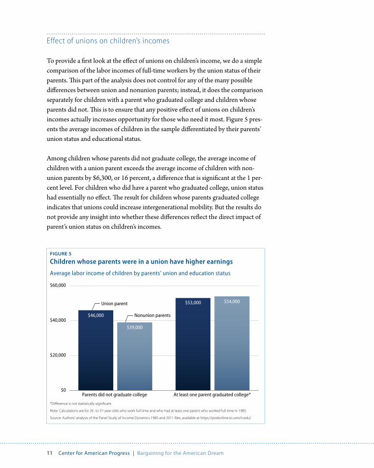
To provide a first look at the effect of unions on children’s income, we do a simple comparison of the labor incomes of full-time workers by the union status of their parents. This part of the analysis does not control for any of the many possible differences between union and nonunion parents; instead, it does the comparison separately for children with a parent who graduated college and children whose parents did not. This is to ensure that any positive effect of unions on children’s incomes actually increases opportunity for those who need it most. Figure 5 pres-ents the average incomes of children in the sample differentiated by their parents’ union status and educational status.

Among children whose parents did not graduate college, the average income of children with a union parent exceeds the average income of children with non-union parents by $6,300, or 16 percent, a difference that is significant at the 1 per-cent level. For children who did have a parent who graduated college, union status had essentially no effect. The result for children whose parents graduated college indicates that unions could increase intergenerational mobility. But the results do not provide any insight into whether these differences reflect the direct impact of parent’s union status on children’s incomes.

*Di�erence is not statistically signi�cant

Note: Calculations are for 26- to 37-year-olds who work full time and who had at least one parent who worked full time in 1985.

Source: Authors' analysis of the Panel Study of Income Dynamics 1985 and 2011 �les, available at https://psidonline.isr.umich.edu/.

FIGURE 5

Children whose parents were in a union have higher earnings

Average labor income of children by parents’ union and education status

Parents did not graduate college At least one parent graduated college*

Union parent

Nonunion parents

$0

$20,000

$40,000

$60,000

$46,000

$39,000

$53,000 $54,000


For this report, we perform a regression analysis that controls for several char-acteristics of the parents that affect their income to allow for an apples-to-apples comparison between union and nonunion parents: race, ethnicity, marital status, education, age, urbanization, occupation, full-time status, and industry. We find that the effect of having a father in a union is an 18.7 percent increase in a child’s earnings, an effect that is significant at the 1 percent level. Next, we control for the income of the parents to examine if there are other ways that parents’ union status affects mobility outside of higher parental incomes. Based on the findings, a union father still increases an offspring’s income by a statistically significant 16.4 percent. When the sample is divided into sons and daughters, one finds that union fathers have positive effects on both sons and daughters. Union mothers, on the other hand, have a positive effect on daughters’ earnings but have no effect on sons. We also find that union membership of the parents raises the incomes of children independent of the child’s own union status.

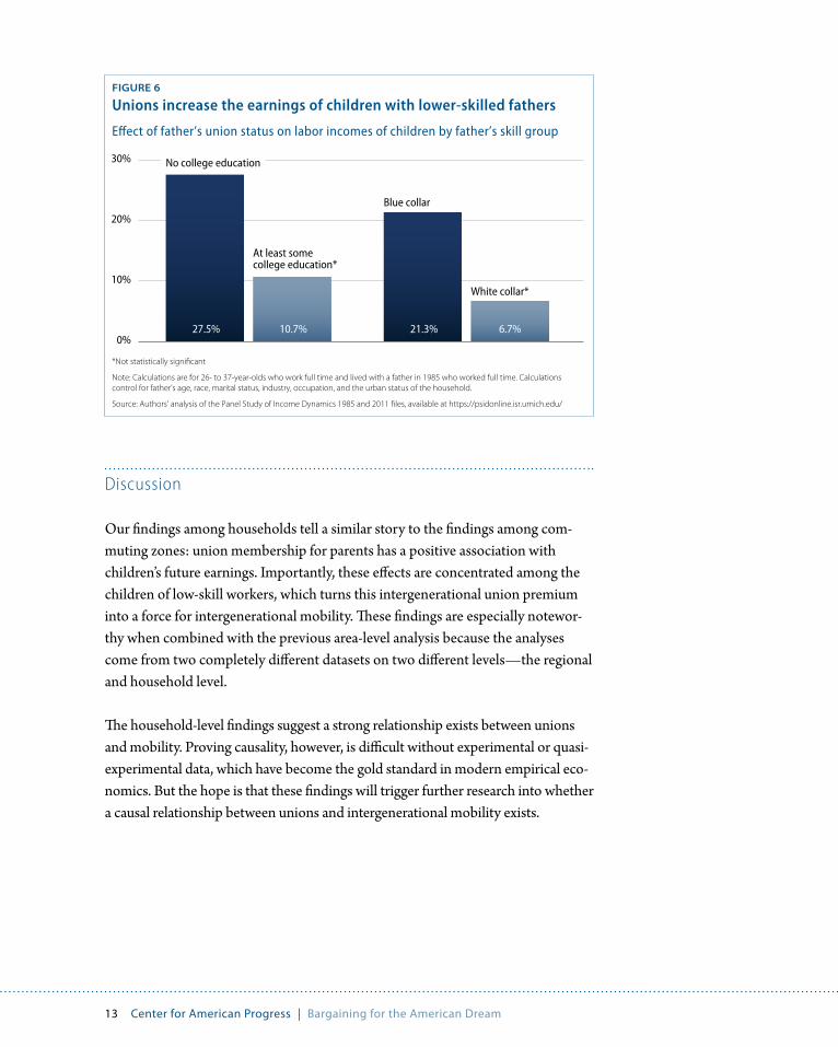
The fact that unions increase the earnings of children does not necessarily mean they boost intergenerational mobility in relative terms; the question is whether unions boost the earnings of the children of higher-skilled or lower-skilled parents. We do this by dividing our sample into approximately equally sized skill groups based on the skill status of the father. The first comparison is for fathers who attended college and fathers who did not. The second comparison is for fathers in blue-collar jobs and fathers in white-collar jobs.

We find that the effects of fathers’ union status are concentrated among the chil-dren of lower-skilled fathers. For sons with a father who did not attend college, unions boost earnings by 27.5 percent, and children of a father with a blue-collar job see a 21.3 percent earnings increase. On the other hand, unions do not have statistically significant effects on children with college-educated fathers or white-collar fathers. The benefits of parents’ union status are thus concentrated among the children of lower-skilled parents, implying that unions increase relative inter-generational mobility.

We also examine two other measures of mobility—the health and education of the children. We measure education by years of school completed and find that a father in a union is associated with completing an additional half year of educa-tion. We measure the effect of unions on health using a five-point scale for self-reported health, 1 being lowest and 5 being highest. We find both union fathers and mothers are associated with statistically significant increases of 0.14 and 0.16 points, respectively.11


Discussion

Our findings among households tell a similar story to the findings among com-muting zones: union membership for parents has a positive association with children’s future earnings. Importantly, these effects are concentrated among the children of low-skill workers, which turns this intergenerational union premium into a force for intergenerational mobility. These findings are especially notewor-thy when combined with the previous area-level analysis because the analyses come from two completely different datasets on two different levels—the regional and household level.

The household-level findings suggest a strong relationship exists between unions and mobility. Proving causality, however, is difficult without experimental or quasi-experimental data, which have become the gold standard in modern empirical eco-nomics. But the hope is that these findings will trigger further research into whether a causal relationship between unions and intergenerational mobility exists.

0%

10%

20%

30%

*Not statistically signi�cant

Note: Calculations are for 26- to 37-year-olds who work full time and lived with a father in 1985 who worked full time. Calculations control for father’s age, race, marital status, industry, occupation, and the urban status of the household.

Source: Authors' analysis of the Panel Study of Income Dynamics 1985 and 2011 �les, available at https://psidonline.isr.umich.edu/

FIGURE 6

Unions increase the earnings of children with lower-skilled fathers

Effect of father’s union status on labor incomes of children by father’s skill group

No college education

Blue collar

White collar*

At least some college education*

27.5% 10.7% 21.3% 6.7%


Unions and stagnant intergenerational mobility

If unions boost intergenerational mobility and they have declined so much over the past 40 years, should economic mobility have fallen? Chetty and his co-authors analyze the time trend of another measure of mobility—the probability that a child born in the bottom quintile would reach the top quintile—and they find that it did not decline between the 1973 and 1993 birth cohorts, a period over which income inequality grew and unionization fell.12 At first glance, this presents a puzzle for our finding that unionization is associated with intergenerational mobility, as well as for Chetty and others’ finding with respect to income equality.

But this puzzle only exists if one believes that declining union membership and growing income inequality were the only trends that affected mobility over the past 40 years. Chetty and his co-authors find that high school dropout rates and racial segregation have declined, offsetting the decline in mobility one would predict based on rising inequality and single motherhood rates:

We predict the trend in the rank-rank slope [relative mobility] implied by changes in the five key correlates over time … The predicted changes are quite small because the factors move in opposing directions. For example, the increase in inequality and single parenthood rates in recent decades predict a small decline in mobility in recent decades. In contrast, the decline in racial segregation and high school dropout rates predict an increase in mobility of similar mag-nitude. Overall, the cross-sectional correlations documented here are consistent with the lack of a substantial time trend in mobility in recent decades.13

Chetty has also noted elsewhere that mobility should have grown in a period of falling racial discrimination and the War on Poverty.14 Mobility did not rise between the early 1970s and early 1990s despite trends that Chetty and his co-authors’ data suggest should have increased mobility—increasing educational attainment, declining segregation, and federal programs targeted at reducing pov-erty. If these trends had not occurred, falling union membership along with rising inequality and single motherhood rates would likely have pushed down mobility.


It is also important to examine the trend in mobility over a longer time period since 20 years is a relatively short span. In a recent National Bureau of Economic Research, or NBER, working paper, Brown University economist Nathaniel Hilger examines educational mobility using U.S. Census Bureau data going all the way back to 1940.15 He also finds that mobility as measured by child educational attainment did not change among 22- to 25-year olds between 1980 and 2000, but this comes after 40 years of growing mobility between 1940 and 1980.16 In other words, the failure of intergenerational mobility to grow between 1980 and 2000 represents a change from rising mobility in the decades before. Moreover, as Harvard political scientist Robert Putnam has argued, it may take time for the full effects of growing inequality to be reflected in mobility statistics if a causal relationship exists.17 The same could be true for unions.

Our findings from both the area and household levels suggest that the decline of union density over the past 40 years along with the increase in inequality and rise of single mothers played a role in preventing mobility from rising. What this implies about the future trend for economic mobility is discouraging unless one expects a continued decline in high school dropout rates and further reduction in racial segregation to offset the effects of rising inequality and falling union membership.


Conclusion

In this report, we have shown that parents’ union membership has a significant and positive relationship with their children’s well-being. The adult offspring of unionized parents earn higher labor incomes compared to the offspring of nonunionized parents. They also attain higher levels of education, which can help them achieve better economic standings. This intergenerational union effect is stronger for less-educated and less-skilled parents, making it a positive force for intergenerational mobility. An association also appears on the area level: Localities with higher union membership are also areas where children of poor parents end up higher in the national income distribution and children throughout the income distribution earn more in these areas.

The research in this report is the first to examine the relationship between unions and intergenerational mobility, but hopefully it will not be the last study on this topic. Researchers have produced a plethora of studies on how falling union membership has increased income inequality, and this report will hopefully inspire others to examine the relationship between unions and mobility in greater detail.

This report also provides lessons for policymakers who have, at least rhetorically, embraced the concept of intergenerational mobility. A serious policy agenda aimed at boosting intergenerational mobility must include policies that will increase the bargaining power of workers. The results from this report show that unions are a powerful force for improving the economic lives not just of organized workers, but of their offspring as well. It is possible that a strong union movement is not simply sufficient for high levels of intergenerational mobility, but it may be necessary. If that is the case, it will be difficult to meaningfully increase intergen-erational mobility without also rebuilding unions or some comparable worker-based organizations.


Appendix A: Area-level data

To perform the analysis of unions and commuting zones, we linked two area-level datasets. The first comes from the “Intergenerational Mobility Statistics and Selected Covariates by County,” developed by Chetty and his co-authors from which mobility for low-income and all children data were obtained (available at www.Equality-of-Opportunity.org). The second dataset is Barry Hirsch and David McPherson’s Current Population Survey-based estimates of union density for metropolitan statistical areas (available at www.UnionStats.com).

Matching the two datasets involved some technical complications. The mobil-ity and income data relate to counties and commuting zones, or CZs, which are themselves collections of counties. The union data are available on the metropoli-tan statistical area, or MSA, level, which are also collections of counties—except in New England, as described below. The geographic analysis takes place on the CZ level. The primary advantage of CZs over MSAs is that the CZ file comes with state identification, which allows for the use of standard errors clustered at the state level to account for spatial and state-specific correlations. Both CZ and MSAs often cross state boundaries—for example, the Washington, D.C., MSA and CZ cover counties in the District of Columbia, Virginia, and Maryland. But the MSAs do not have state IDs, and thus we cannot use state clustered standard errors with them. We assign to each county the union density of the MSA to which it belongs and then combines the counties into CZs, dropping counties that are not part of MSAs since there are no union data for them. This removes rural counties from CZs and creates some slight differences in the covariates from the original data featured in Chetty’s paper. But we do not believe this is a serious problem: the correlation between mobility for low-income children estimates of our limited CZs and the whole CZs is 0.946. Additionally, we reconstruct the covariates on the CZ-level only for counties for which there are also union data. The correlation between the five factors in our limited CZs and the whole CZs ranges between 0.937 and 0.980.

http://www.Equality-of-Opportunity.org

http://www.UnionStats.com


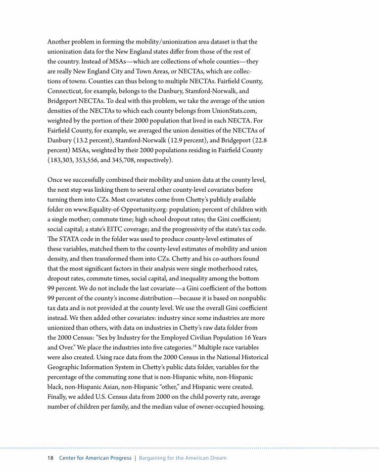
Another problem in forming the mobility/unionization area dataset is that the unionization data for the New England states differ from those of the rest of the country. Instead of MSAs—which are collections of whole counties—they are really New England City and Town Areas, or NECTAs, which are collec-tions of towns. Counties can thus belong to multiple NECTAs. Fairfield County, Connecticut, for example, belongs to the Danbury, Stamford-Norwalk, and Bridgeport NECTAs. To deal with this problem, we take the average of the union densities of the NECTAs to which each county belongs from UnionStats.com, weighted by the portion of their 2000 population that lived in each NECTA. For Fairfield County, for example, we averaged the union densities of the NECTAs of Danbury (13.2 percent), Stamford-Norwalk (12.9 percent), and Bridgeport (22.8 percent) MSAs, weighted by their 2000 populations residing in Fairfield County (183,303, 353,556, and 345,708, respectively).

Once we successfully combined their mobility and union data at the county level, the next step was linking them to several other county-level covariates before turning them into CZs. Most covariates come from Chetty’s publicly available folder on www.Equality-of-Opportunity.org: population; percent of children with a single mother; commute time; high school dropout rates; the Gini coefficient; social capital; a state’s EITC coverage; and the progressivity of the state’s tax code. The STATA code in the folder was used to produce county-level estimates of these variables, matched them to the county-level estimates of mobility and union density, and then transformed them into CZs. Chetty and his co-authors found that the most significant factors in their analysis were single motherhood rates, dropout rates, commute times, social capital, and inequality among the bottom 99 percent. We do not include the last covariate—a Gini coefficient of the bottom 99 percent of the county’s income distribution—because it is based on nonpublic tax data and is not provided at the county level. We use the overall Gini coefficient instead. We then added other covariates: industry since some industries are more unionized than others, with data on industries in Chetty’s raw data folder from the 2000 Census: ”Sex by Industry for the Employed Civilian Population 16 Years and Over.” We place the industries into five categories.18 Multiple race variables were also created. Using race data from the 2000 Census in the National Historical Geographic Information System in Chetty’s public data folder, variables for the percentage of the commuting zone that is non-Hispanic white, non-Hispanic black, non-Hispanic Asian, non-Hispanic “other,” and Hispanic were created. Finally, we added U.S. Census data from 2000 on the child poverty rate, average number of children per family, and the median value of owner-occupied housing.

http://www.Equality-of-Opportunity.org


Once we combined union, mobility, and other covariate data on the county level, we turned them into CZs. Lacking union data outside of MSAs, this analysis does not apply to rural areas. The total population of our CZs in 2000 was 207 million people compared to a U.S. population of 281 million in 2000.19 There is no way to obtain unionization rates for rural areas to see whether the results of this report do or do not hold for these areas.


Appendix B: Area-level analysis

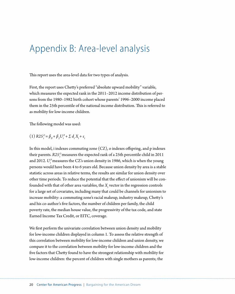
This report uses the area-level data for two types of analysis.

First, the report uses Chetty’s preferred “absolute upward mobility” variable, which measures the expected rank in the 2011–2012 income distribution of per-sons from the 1980–1982 birth cohort whose parents’ 1996–2000 income placed them in the 25th percentile of the national income distribution. This is referred to as mobility for low-income children.

The following model was used:

(1) R25iO = β0 + β1Ui

P + ∑ di Xi + εi

In this model, i indexes commuting zone (CZ), o indexes offspring, and p indexes their parents. R25i

O measures the expected rank of a 25th percentile child in 2011 and 2012. Ui

P measures the CZ’s union density in 1986, which is when the young persons would have been 4 to 6 years old. Because union density by area is a stable statistic across areas in relative terms, the results are similar for union density over other time periods. To reduce the potential that the effect of unionism will be con-founded with that of other area variables, the Xi vector in the regression controls for a large set of covariates, including many that could be channels for unionism to increase mobility: a commuting zone’s racial makeup, industry makeup, Chetty’s and his co-author’s five factors, the number of children per family, the child poverty rate, the median house value, the progressivity of the tax code, and state Earned Income Tax Credit, or EITC, coverage.

We first perform the univariate correlation between union density and mobility for low-income children displayed in column 1. To assess the relative strength of this correlation between mobility for low-income children and union density, we compare it to the correlation between mobility for low-income children and the five factors that Chetty found to have the strongest relationship with mobility for low-income children: the percent of children with single mothers as parents; the


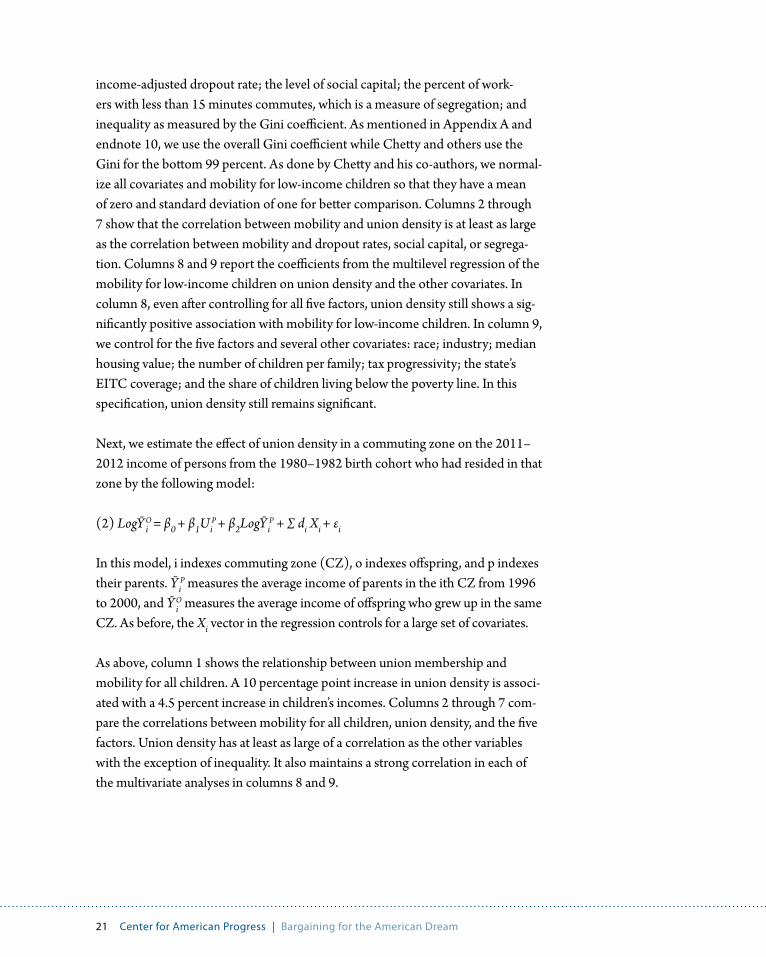
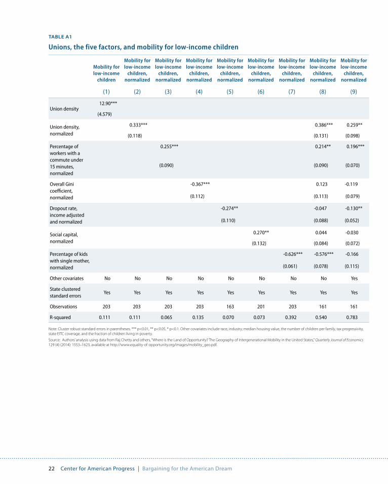
income-adjusted dropout rate; the level of social capital; the percent of work-ers with less than 15 minutes commutes, which is a measure of segregation; and inequality as measured by the Gini coefficient. As mentioned in Appendix A and endnote 10, we use the overall Gini coefficient while Chetty and others use the Gini for the bottom 99 percent. As done by Chetty and his co-authors, we normal-ize all covariates and mobility for low-income children so that they have a mean of zero and standard deviation of one for better comparison. Columns 2 through 7 show that the correlation between mobility and union density is at least as large as the correlation between mobility and dropout rates, social capital, or segrega-tion. Columns 8 and 9 report the coefficients from the multilevel regression of the mobility for low-income children on union density and the other covariates. In column 8, even after controlling for all five factors, union density still shows a sig-nificantly positive association with mobility for low-income children. In column 9, we control for the five factors and several other covariates: race; industry; median housing value; the number of children per family; tax progressivity; the state’s EITC coverage; and the share of children living below the poverty line. In this specification, union density still remains significant.

Next, we estimate the effect of union density in a commuting zone on the 2011–2012 income of persons from the 1980–1982 birth cohort who had resided in that zone by the following model:

(2) LogȲ iO = β0 + β1Ui

P + β2LogȲiP + ∑ di Xi + εi

In this model, i indexes commuting zone (CZ), o indexes offspring, and p indexes their parents. Ȳi

P measures the average income of parents in the ith CZ from 1996 to 2000, and Ȳ i

O measures the average income of offspring who grew up in the same CZ. As before, the Xi vector in the regression controls for a large set of covariates.

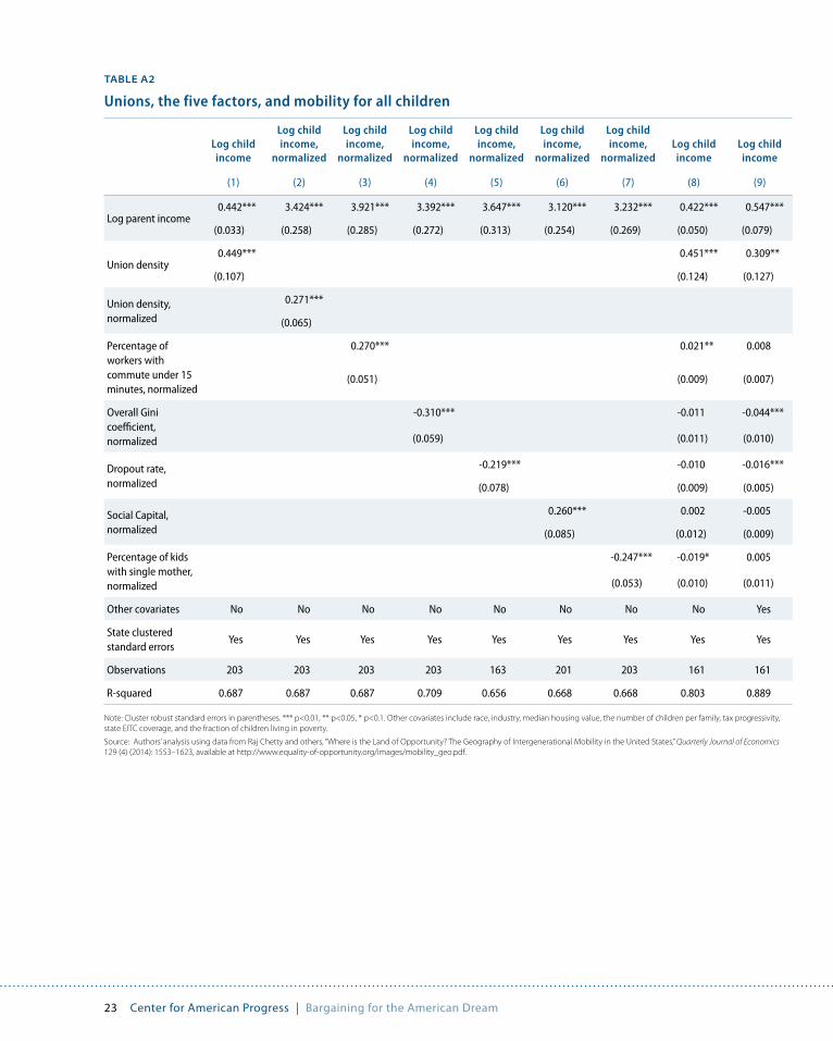
As above, column 1 shows the relationship between union membership and mobility for all children. A 10 percentage point increase in union density is associ-ated with a 4.5 percent increase in children’s incomes. Columns 2 through 7 com-pare the correlations between mobility for all children, union density, and the five factors. Union density has at least as large of a correlation as the other variables with the exception of inequality. It also maintains a strong correlation in each of the multivariate analyses in columns 8 and 9.


TABLE A1

Unions, the five factors, and mobility for low-income children

Mobility for low-income

children


children, normalized















(1) (2) (3) (4) (5) (6) (7) (8) (9)

Union density12.90***

(4.579)

Union density, normalized

0.333*** 0.386*** 0.259**

(0.118) (0.131) (0.098)

Percentage of workers with a commute under 15 minutes, normalized

0.255*** 0.214** 0.196***

(0.090) (0.090) (0.070)

Overall Gini coefficient, normalized

-0.367*** 0.123 -0.119

(0.112) (0.113) (0.079)

Dropout rate, income adjusted and normalized

-0.274** -0.047 -0.130**

(0.110) (0.088) (0.052)

Social capital, normalized

0.270** 0.044 -0.030

(0.132) (0.084) (0.072)

Percentage of kids with single mother, normalized

-0.626*** -0.576*** -0.166

(0.061) (0.078) (0.115)

Other covariates No No No No No No No No Yes

State clustered standard errors

Yes Yes Yes Yes Yes Yes Yes Yes Yes

Observations 203 203 203 203 163 201 203 161 161

R-squared 0.111 0.111 0.065 0.135 0.070 0.073 0.392 0.540 0.783

Note: Cluster robust standard errors in parentheses. *** p<0.01, ** p<0.05, * p<0.1. Other covariates include race, industry, median housing value, the number of children per family, tax progressivity, state EITC coverage, and the fraction of children living in poverty.

Source: Authors’ analysis using data from Raj Chetty and others, “Where is the Land of Opportunity? The Geography of Intergenerational Mobility in the United States,” Quarterly Journal of Economics 129 (4) (2014): 1553–1623, available at http://www.equality-of-opportunity.org/images/mobility_geo.pdf.


TABLE A2

Unions, the five factors, and mobility for all children

Log child income

Log child income,

normalized

Log child income,

normalized

Log child income,

normalized

Log child income,

normalized

Log child income,

normalized

Log child income,

normalizedLog child income

Log child income

(1) (2) (3) (4) (5) (6) (7) (8) (9)

Log parent income0.442*** 3.424*** 3.921*** 3.392*** 3.647*** 3.120*** 3.232*** 0.422*** 0.547***

(0.033) (0.258) (0.285) (0.272) (0.313) (0.254) (0.269) (0.050) (0.079)

Union density0.449*** 0.451*** 0.309**

(0.107) (0.124) (0.127)

Union density, normalized

0.271***

(0.065)

Percentage of workers with commute under 15 minutes, normalized

0.270*** 0.021** 0.008

(0.051) (0.009) (0.007)

Overall Gini coefficient, normalized

-0.310*** -0.011 -0.044***

(0.059) (0.011) (0.010)

Dropout rate, normalized

-0.219*** -0.010 -0.016***

(0.078) (0.009) (0.005)

Social Capital, normalized

0.260*** 0.002 -0.005

(0.085) (0.012) (0.009)

Percentage of kids with single mother, normalized

-0.247*** -0.019* 0.005

(0.053) (0.010) (0.011)

Other covariates No No No No No No No No Yes


Yes Yes Yes Yes Yes Yes Yes Yes Yes

Observations 203 203 203 203 163 201 203 161 161

R-squared 0.687 0.687 0.687 0.709 0.656 0.668 0.668 0.803 0.889

Note: Cluster robust standard errors in parentheses. *** p<0.01, ** p<0.05, * p<0.1. Other covariates include race, industry, median housing value, the number of children per family, tax progressivity, state EITC coverage, and the fraction of children living in poverty.

Source: Authors’ analysis using data from Raj Chetty and others, “Where is the Land of Opportunity? The Geography of Intergenerational Mobility in the United States,” Quarterly Journal of Economics 129 (4) (2014): 1553–1623, available at http://www.equality-of-opportunity.org/images/mobility_geo.pdf.


Appendix C: Individual household data and analysis

The Panel Study of Income Dynamics, or PSID, provides detail on the characteris-tics of families, including the labor income and union status of the head of house-hold and of the head’s spouse and the comparable characteristics of their adult offspring when they form their own households. To obtain a sample of parents and their adult offspring, we matched the 1985 and 2011 PSID files by individual and created a new file limited to individuals who were children or stepchildren of the head of a household in 1985 and were themselves heads of household or the spouses of household heads in 2011. We also restrict the sample to those younger than 38 years old in 2011—younger than 12 years old in 1985—so that they are young enough to be directly influenced by parents’ economic status. We created a new set of 2011 offspring variables to characterize this group: characteristics of the household heads if the individual was the head of household and characteristics of the wives if the individual was the married or unmarried partner of the household head. These offspring variables are designed to focus on the relationships between parents and their children rather than between parents and the spouses of their children. Because we limit their analysis to heads of household and spouses, the data exclude children who were not heads of household or spouses, which consist primarily of those living with their parents in 2011.

We regress the log of offspring income on the log of their parental income and other parental characteristics using the following form:

(3) LogYjk = β0 + β1UkP + β2 LogYk

P + ∑ dk XkP + εjk

In this model, j indexes offspring and k indexes their parents. Y is offspring’s labor income.20 UP is their parents’ union status, where 1 means the parents are union-ized and 0 that they are not in a union. YP is parents’ family income and XP rep-resents other parental attributes: parents’ age; race and ethnicity; their full-time status; education; marital status; industry and occupations; and the urban status of the household. If UP is significantly positive, then on average, the offspring of union parents earn higher incomes than the offspring of nonunion parents.


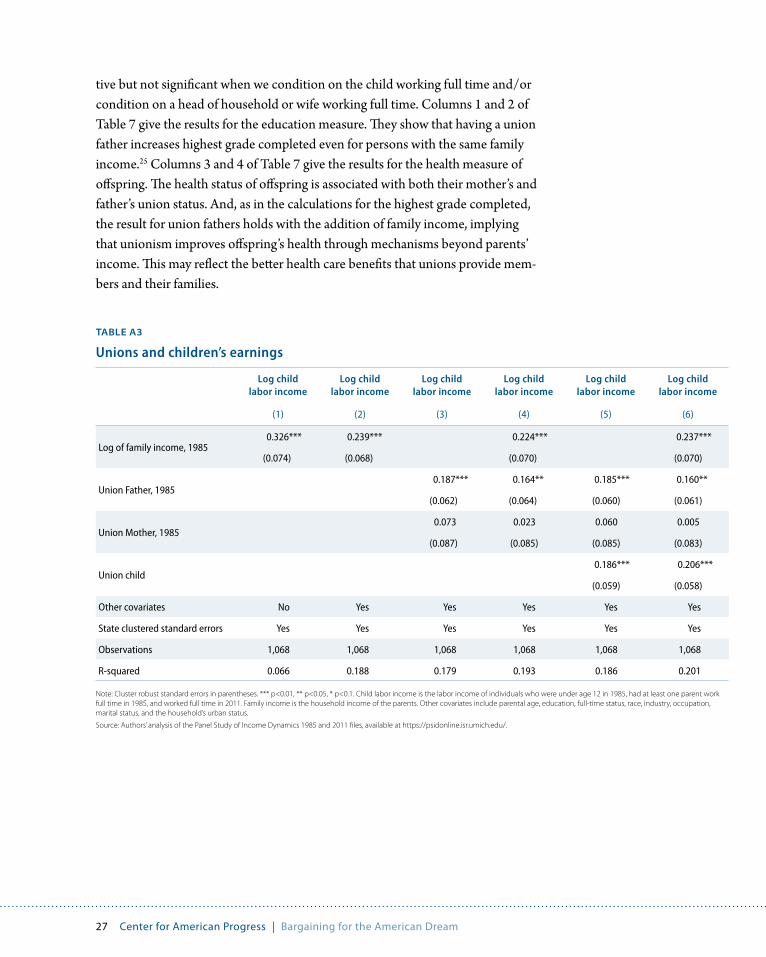
Table 3 gives the results of the regressions of the log of offspring income on par-ents’ attributes, including parents’ family income.21 The coefficient on the log of family income in column 1 is the intergenerational income elasticity, or IGE, that measures the association between parents’ income and their offspring’s income.22 The estimated coefficient of 0.326 indicates that if parents’ income increases by 10 percent, offspring’s labor income increases by 3.3 percent for all persons in the sample.23 The addition of the covariates for parental attributes reduces the coef-ficient to 0.239 in column 2.

Column 3 examines the effect of having union parents on offspring income absent family income but with inclusion of other parental covariates and deliv-ers our main finding from the individual-level data: the father’s union status has a significant effect on child income with a magnitude of 0.187, which implies that the adult offspring of unionized fathers earn 18.7 percent higher income than the adult offspring of nonunionized fathers. The addition of parental family income in column 4 reduces the coefficient on the union status of parental-household head to 0.164. This implies that the effect of parents’ unionism goes beyond their higher income due to the union premium.

Finally, in columns 5 and 6, we add a dummy variable indicating whether the offspring are unionized. The estimated coefficients on parental union status and parental income do not change much after we include offspring’s union status, which suggests that parents’ union status has an independently positive impact on their children’s income beyond whether their children join a union. The estimated coefficient on children’s union status shows that they earn a substantial union pre-mium. Compared to children whose parents and themselves have no connection to unionism, children whose parents are unionized and themselves are also union-ized earn about 37 percent (18.5 percent + 18.6 percent) higher labor incomes. We also analyzed the effect of parents’ unionism controlling for separate labor incomes of household heads and their spouses rather than controlling for parent’s family income, and we find an even higher efficient coefficient on union fathers.24

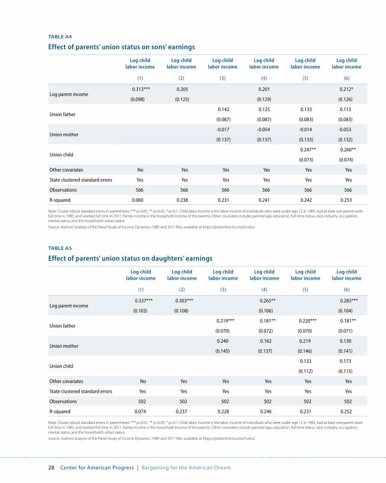
We also examine the effects of mothers’ and fathers’ union status on daughters and sons separately in Tables 4 and 5. The relationship is less precisely estimated than the above regressions since the sample size is about half. The point estimates for the effect of fathers’ union status on sons are slightly smaller than in the pooled samples while, mothers’ union status appears to have no effect on sons’ labor incomes. For daughters, we find the effects of fathers’ union status are larger than those for sons, and the effect of mothers’ union status is also positive but not quite significant.


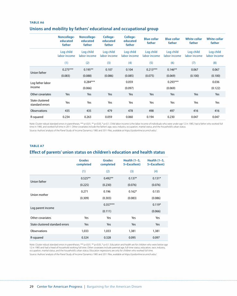
Given the many pathways that educated and skilled workers are likely to have to pass on their economic advantages to their children, it is important to determine whether the union parents’ effect on their offspring’s income is stronger among less-educated and less-skilled workers than among more-educated and more-skilled workers. In the former case, the union effect would reduce relative social mobility while in the latter case the union effect would increase relative mobility.

To examine this issue, we divided their sample by level of education—fathers with no college education and those with at least some college education—and by nature of work—fathers in blue-collar occupations compared to fathers in white-collar occupations—and estimated equation 3 and 4 for these groups. We only examine fathers in order to avoid the complications of marriages where one partner has a college education or a white-collar job while the other has no college education or a blue-collar job. We used at least some college as the cutoff because roughly half of fathers had some college education, and the cutoff thus maximizes sample size for both groups. The results, summarized in Table 6 show that the union effect in raising the income of offspring is concentrated among fathers with less education and among fathers in blue-collar jobs. While one potential explana-tion is the large union wage premium for low-skilled workers, the inclusion of the parental household income variable, which should reflect the wage premium, still leaves a sizable independent union effect.

Our final research question in the individual-level data is what extent does the effect of parents’ unionism show up in other measures of socioeconomic well-being? We examine this question by estimating variants of equations 3 and 4 that replace children’s labor income with measures of educational progress—highest grade completed—and health, as reported by individuals on a 1 to 5 scale with 5 as the best health and 1 as the worst health status.

For the health and education regressions, we condition on a head of household who works full time rather than a head of household or wife that works full time as in the other regressions. This is in order to capture unions’ potential role on mother’s well-being through better maternity leave since a mother on maternity leave would not be counted as working full time. Unlike all the other results—including the education results—the health results are sensitive to this adjustment and do not display significant effects if we condition on either the household head or wife working full time. We also drop the requirement for the health regressions that the children work full time since the beneficial effects of unions on children’s health should not depend on their labor market status. The health results are posi-


tive but not significant when we condition on the child working full time and/or condition on a head of household or wife working full time. Columns 1 and 2 of Table 7 give the results for the education measure. They show that having a union father increases highest grade completed even for persons with the same family income.25 Columns 3 and 4 of Table 7 give the results for the health measure of offspring. The health status of offspring is associated with both their mother’s and father’s union status. And, as in the calculations for the highest grade completed, the result for union fathers holds with the addition of family income, implying that unionism improves offspring’s health through mechanisms beyond parents’ income. This may reflect the better health care benefits that unions provide mem-bers and their families.

TABLE A3

Unions and children’s earnings

Log child labor income






(1) (2) (3) (4) (5) (6)

Log of family income, 19850.326*** 0.239*** 0.224*** 0.237***

(0.074) (0.068) (0.070) (0.070)

Union Father, 19850.187*** 0.164** 0.185*** 0.160**

(0.062) (0.064) (0.060) (0.061)

Union Mother, 19850.073 0.023 0.060 0.005

(0.087) (0.085) (0.085) (0.083)

Union child0.186*** 0.206***

(0.059) (0.058)

Other covariates No Yes Yes Yes Yes Yes

State clustered standard errors Yes Yes Yes Yes Yes Yes

Observations 1,068 1,068 1,068 1,068 1,068 1,068

R-squared 0.066 0.188 0.179 0.193 0.186 0.201

Note: Cluster robust standard errors in parentheses. *** p<0.01, ** p<0.05, * p<0.1. Child labor income is the labor income of individuals who were under age 12 in 1985, had at least one parent work full time in 1985, and worked full time in 2011. Family income is the household income of the parents. Other covariates include parental age, education, full-time status, race, industry, occupation, marital status, and the household’s urban status.

Source: Authors’ analysis of the Panel Study of Income Dynamics 1985 and 2011 files, available at https://psidonline.isr.umich.edu/.


TABLE A4

Effect of parents’ union status on sons’ earnings







(1) (2) (3) (4) (5) (6)

Log parent income0.313*** 0.205 0.201 0.212*

(0.098) (0.125) (0.129) (0.126)

Union father0.142 0.125 0.133 0.115

(0.087) (0.087) (0.083) (0.083)

Union mother-0.017 -0.054 -0.014 -0.053

(0.137) (0.137) (0.133) (0.132)

Union child0.247** 0.260**

(0.073) (0.074)



Observations 566 566 566 566 566 566

R-squared 0.060 0.238 0.231 0.241 0.242 0.253



TABLE A5

Effect of parents’ union status on daughters’ earnings







(1) (2) (3) (4) (5) (6)

Log parent income0.337*** 0.303*** 0.265** 0.283***

(0.103) (0.108) (0.106) (0.104)

Union father0.219*** 0.181** 0.220*** 0.181**

(0.070) (0.072) (0.070) (0.071)

Union mother0.240 0.162 0.219 0.130

(0.145) (0.137) (0.146) (0.141)

Union child0.133 0.173

(0.112) (0.115)



Observations 502 502 502 502 502 502

R-squared 0.074 0.237 0.228 0.246 0.231 0.252




TABLE A6

Unions and mobility by fathers’ educational and occupational group

Noncollege-educated

father

Noncollege-educated

father

College- educated

father

College- educated

father

Blue collar father

Blue collar father

White collar father

White collar father









(1) (2) (3) (4) (5) (6) (7) (8)

Union father0.275*** 0.195** 0.107 0.104 0.213*** 0.146** 0.067 0.067

(0.083) (0.088) (0.086) (0.085) (0.075) (0.069) (0.100) (0.100)

Log father labor income

0.284*** 0.059 0.293*** 0.036

(0.066) (0.097) (0.069) (0.122)

Other covariates Yes Yes Yes Yes Yes Yes Yes Yes


Yes Yes Yes Yes Yes Yes Yes Yes

Observations 435 435 479 478 498 497 416 416

R-squared 0.234 0.263 0.059 0.060 0.194 0.230 0.047 0.047

Note: Cluster robust standard errors in parentheses. *** p<0.01, ** p<0.05, * p<0.1. Child labor income is the labor income of individuals who were under age 12 in 1985, had a father who worked full time in 1985, and worked full time in 2011. Other covariates include the father’s age, race, industry, occupation, marital status, and the household’s urban status.


TABLE A7

Effect of parents’ union status on children’s education and health status

Grades completed

Grades completed

Health (1–5, 5=Excellent)

Health (1–5, 5=Excellent)

(1) (2) (3) (4)

Union father0.525** 0.492** 0.137* 0.131*

(0.225) (0.230) (0.076) (0.076)

Union mother0.271 0.196 0.162* 0.135

(0.309) (0.303) (0.083) (0.086)

Log parent income0.357*** 0.119*

(0.111) (0.066)

Other covariates Yes Yes Yes Yes

State clustered standard errors Yes Yes Yes Yes

Observations 1,033 1,033 1,381 1,381

R-squared 0.324 0.328 0.095 0.097

Note: Cluster robust standard errors in parentheses. *** p<0.01, ** p<0.05, * p<0.1. Education and health are for children who were below age 12 in 1985 and had a head of household working full time. Other covariates include parental age, full-time status, education, race, industry, occupation, marital status, and the household’s urban status. Education regressions are only for children who worked full time.



About the authors

Richard Freeman holds the Herbert Ascherman chair in economics at Harvard University and is a research associate at the National Bureau of Economic Research in Cambridge, Massachusetts.

Eunice Han is a professor of economics at Wellesley College and a research fellow at the National Bureau of Economic Research. Her research covers topics in labor economics and the economics of education with an emphasis on institutions and legal systems. She currently focuses on the impact of unionism on the local labor market, especially with regards to income inequality and economic mobility. She received her Ph.D. in economics from Harvard University in 2013.

David Madland is the Managing Director of the Economic Policy team and the Director of the American Worker Project at Center for American Progress. He has written extensively about the economy and American politics on a range of topics, including the middle class, economic inequality, retirement policy, labor unions, and workplace standards such as the minimum wage. His book, Hollowed Out: Why the Economy Doesn’t Work without a Strong Middle Class, was published by the University of California Press in June 2015. Madland has a doctorate in govern-ment from Georgetown University and received his bachelor’s degree from the University of California, Berkeley.

Brendan V. Duke is a Policy Analyst for the Center for American Progress’ Middle-Out Economics project. His research focuses on economic inequality and eco-nomic growth. He holds a master’s degree in economics and public policy from Princeton University’s Woodrow Wilson School of Public and International Affairs.


Endnotes

1 Raj Chetty, Nathaniel Hendren, Patrick Kline, and Em-manuel Saez, “Where is the Land of Opportunity? The Geography of Intergenerational Mobility in the United States,” Quarterly Journal of Economics 129 (4) (2014): 1553–1623.

2 Ibid.

3 David Madland and Nick Bunker, “Unions Boost Economic Mobility in U.S. States” (Washington: Center for American Progress Action Fund, 2012), available at https://www.americanprogressaction.org/issues/labor/report/2012/09/20/38624/unions-boost-economic-mobility-in-u-s-states/.

4 Bruce Western and Jake Rosenfeld, “How Much Has De-Unionisation Contributed to the Rise in Male Earn-ings Inequality,” The American Sociological Review 4 (76) (2011): 513–537; David Card, Thomas Lemieux, and W. Craig Riddell, “Unions and Wage Inequality,” Journal of Labor Research 25 (2004); John DiNardo, Nicole M. Fortin, and Thomas Lemieux, “Labor Market Institu-tions and the Distribution of Wages, 1973–1992: A Semiparametric Approach,” Econometrica 5 (64) (1996): 1001-1004; Richard B. Freeman, “How Much Has De-Unionisation Contributed to the Rise in Male Earnings Inequality?” In Sheldon Danziger and Peter Gottschalk (eds.), Uneven Tides (New York: Sage Press, 1992), pp. 133–163.

5 Western and Rosenfeld, “How Much Has De-Unionisa-tion Contributed to the Rise in Male Earnings Inequal-ity.”

6 Unions’ tendency to raise wages for nonunion workers because firms try to avoid unionization is called the threat effect. Unions could also reduce wages for nonunion workers if union wages and benefits reduced employment in the union sector, increasing the labor supply in nonunion work; this is called the crowding effect. Evidence suggests that the threat effect domi-nates the crowding effect and that unions raise wages for nonunion workers. See Henry S. Farber, “Nonunion Wage Rates and the Threat of Unionization,” ILR Review 28 (3) (2005): 335–352.

7 Martin Gilens, Affluence and Influence: Economic Inequality and Political Power in America (Princeton, NJ: Princeton University Press, 2013), pp. 154–160.

8 James Cox and Ronald L. Oaxaca, “The Political Econo-my of Minimum Wage Legislation,” Economic Inquiry 20 (4) (1982): 533–555.

9 Chetty, Hendren, Kline, and Saez, “Where is the Land of Opportunity?”

10 Chetty and others, “Where is the Land of Opportunity?” finds a Gini coefficient of just the bottom 99 percent of households has a stronger negative association with mobility than an overall Gini does and uses this bottom 99 percent Gini as one of its five factors. We use the overall Gini, however, because they do not provide a bottom 99 percent Gini by county (which we need to include it in our analysis because of the complications of combining with the union data), and it comes from their federal tax data, so public data could not be used. See Appendix A for more details.

11 As described in the appendix, the health results are sensitive to the population analyzed. We find positive and statistically significant results when we do not con-dition on the child working full time and only condition

on the head of household working full time (the latter to include union mothers on maternity leave). The health results are positive but not significant when we condition on the child working full time and/or condi-tion on a head of household or wife working full time.

12 Raj Chetty and others, “Is the United States Still a Land of Opportunity? Recent Trends in Intergenerational Mobility,” American Economic Review Papers and Pro-ceedings 104 (5) (2014): 141–147.

13 Chetty, Hendren, Kline, and Saez, “Where is the Land of Opportunity?”

14 Danny Vinik, “Is It Inequality or Mobility? Neither Econo-mists nor GOP Candidates Can Decide,” New Republic, April 7, 2015, available at http://www.newrepublic.com/article/121465/2016-presidential-candidates-face-challenge-talking-about-inequality.

15 Nathaniel G. Hilger, “The Great Escape: Intergenera-tional Mobility Since 1940.” Working Paper 21217 (Cam-bridge, MA: National Bureau of Economic Research, 2015).

16 Ibid.

17 Robert D. Putnam, Our Kids (New York: Simon & Schus-ter, 2015), p. 228.

18 Sectors are based on Zoltan Kenessey, “The Primary, Secondary, Tertiary And Quaternary Sectors Of The Economy,” Review of Income and Wealth 33 (4) (1987): 359–385. Analysis with major industry categories yields similar results.

19 Marc J. Perry and Paul J. Mackun, “Population Change and Distribution” (Washington: U.S. Bureau of the Census, 2001), available at https://www.census.gov/prod/2001pubs/c2kbr01-2.pdf.

20 To measure the direct effect of parents’ unionism on offspring income, the authors focus on offspring’s labor income rather than the combined family income of married couples. The use of labor income drops children who are self-employed status or out of labor force.

21 The full results for all of the authors’ regression analyses are available upon request.

22 It is commonly understood that the higher value of IGE, the lower the intergenerational mobility is. In one extreme case, the IGE would be equal to zero if there exists no relationship between family background and the adult offspring income. Children born into a poor family would have the same likelihood of earning a high income as children born into a rich family.

23 Although the authors used labor income rather than family income of offspring, this estimate is consistent with literature. See Chetty and others, “Where is the Land of Opportunity?”; Chul-In Lee and Gary Solon, “Trends in Intergenerational Income Mobility,” Review of Economics and Statistics 91 (4) (2009): 766-772; Bhashkar Mazumder, “Fortunate Sons: New Estimates of Intergenerational Mobility in the United States Using Social Security Earnings Data,” The Review of Economics and Statistics 87 (2) (2005): 235-255. This literature states that the estimated IGE could be subject to the attenuation bias if the data focus on short-term periods due to the long-lasting transitory shocks to income.

http://www.newrepublic.com/article/121465/2016-presidential-candidates-face-challenge-talking-about-inequality




24 If we control for separate labor incomes of both parents, the coefficients on union father in Model 4, for example, is 0.25 and is statistically significant at the 1 percent of significance level. The coefficient on union mothers remain insignificant.

25 In regressions with high school graduation as the measure of schooling, the father’s unionism raises sons’ high school graduation rate by a statistically significant 4.4 percentage points.

1333 H STREET, NW, 10TH FLOOR, WASHINGTON, DC 20005 • TEL: 202-682-1611 • FAX: 202-682-1867 • WWW.AMERICANPROGRESS.ORG

Our Mission

The Center for American Progress is an independent, nonpartisan policy institute that is dedicated to improving the lives of all Americans, through bold, progressive ideas, as well as strong leadership and concerted action. Our aim is not just to change the conversation, but to change the country.

Our Values

As progressives, we believe America should be a land of boundless opportunity, where people can climb the ladder of economic mobility. We believe we owe it to future generations to protect the planet and promote peace and shared global prosperity.

And we believe an effective government can earn the trust of the American people, champion the common good over narrow self-interest, and harness the strength of our diversity.

Our Approach

We develop new policy ideas, challenge the media to cover the issues that truly matter, and shape the national debate. With policy teams in major issue areas, American Progress can think creatively at the cross-section of traditional boundaries to develop ideas for policymakers that lead to real change. By employing an extensive communications and outreach effort that we adapt to a rapidly changing media landscape, we move our ideas aggressively in the national policy debate.

Documents

Bargaining for the American Dream · Bargaining for the American Dream ... Bargaining for the American Dream Introduction and summary ... study on interest groups and political influence