Banks, Liquidity Management

and Monetary Policy∗

Javier Bianchi

University of Wisconsin and NBER

Saki Bigio

Columbia University

July 2014

Abstract

We develop a new framework to study the implementation of monetary policy through the

banking system. Banks finance illiquid loans by issuing deposits. Deposit transfers across

banks must be settled using central bank reserves. Transfers are random and, therefore,

create liquidity risk. The degree of liquidity risk determines the supply of credit and the

money multiplier. We study how different shocks to the banking system and monetary policy

affect the economy by altering the tradeoff between profiting from lending against incurring

in greater liquidity risk. We calibrate our model to study, quantitatively, why banks have

recently increased their reserve holdings but not expanded loans despite policy efforts. We

find that credit demand shocks are the main driving force.

Keywords: Banks, monetary policy, liquidity, capital requirements

∗We would like to thank Harjoat Bhamra, John Cochrane, Dean Corbae, Itamar Dreschler, Xavier Freixas,Anil Kashyap, Nobu Kiyotaki, Arvind Krishnamurthy, Ricardo Lagos, Thomas Philippon, Chris Phelan, TomekPiskorski, Ricardo Reis, Chris Sims, Harald Uhlig, and Mike Woodford for helpful discussions. We also wish tothank seminar participants at Banque de France, Bank of Italy, Bank of Japan, Central Bank of Chile, Central Bankof Peru, Central Bank of Uruguay, Chicago Fed, Columbia University, the European Central Bank, PhiladelphiaFed the Riksbank, University of Maryland, University of Chicago, Goethe University, Minneapolis Fed, UniversidadCatolica de Chile, SAIF, Yale, and conference participants at the 2nd Rome Junior Conference on Macroeconomicsat the Einaudi Institute, the 2013 Barcelona GSE Summer Forum, the 2nd Macro Finance Society Workshop, theFourth Boston University/Boston Fed Conference on Macro-Finance Linkages, and the CEPR Conference on Banksand Governments in Globalised Financial Markets at Oesterreichische Nationalbank, Workshop on Safe Assets andthe Macroeconomy at London Business School, Society of Economic Dynamics. We are grateful for the financialsupport by the Fondation Banque de France. Emails: jibianchi@wisc.edu and sbigio@columbia.edu.

1

1 Introduction

The conduct of monetary policy around the world is changing. The past five years have witnessed

banking systems that bore unprecedented financial losses and subsequent freezes in interbank mar-

kets. Following these events, there was a major reduction in bank lending followed by a protracted

recession. In response, central banks in developed economies have reduced policy rates to almost

zero and expanded their balance sheets in an open attempt to preserve financial stability and rein-

vigorate lending. However, in reaction to these unprecedented policy interventions, banks seem

to have accumulated central bank reserves without renewing their lending activities as intended.1

Why? Can central banks do more about this? These remain open questions.

Not surprisingly, the role of banks in the transmission of monetary policy has been at the

center of policy debates. However, there are few modern macroeconomic models that take into

account that monetary policy is implemented through the banking system, as occurs in practice.

Instead, most macroeconomic models assume that central banks control interest rates or mone-

tary aggregates and abstract from how the transmission of monetary policy may depend on the

conditions of banks. This paper presents a model that contributes to fill in this gap.

The Mechanism. The building block of our model is a liquidity management problem.

Liquidity management is recognized as one of the fundamental problems in banking and can be

explained as follows. When a bank grants a loan, it simultaneously creates demand deposits —or

credit lines. These deposits can be used by the borrower to perform transactions at any time.

Granting a loan is profitable because a higher interest is charged on the loan than what is paid

on deposits. However, more lending relative to a given amount of central bank reserves increases

a bank’s liquidity risk. When deposits are transferred out of a bank, that bank must transfer

reserves to other banks in order to settle transactions. Central bank reserves are critical to clear

settlements because loans cannot be sold immediately. Thus, the lower the reserve holdings of a

bank, the more likely it is to be short of reserves in the future. This is a source of risk because the

bank must incur expensive borrowing from other banks —or the central bank’s discount window—

if it falls short of reserves. This friction —the liquidity mismatch— induces a tradeoff between

profiting from lending and incurring additional liquidity risks which we call liquidity management.

It is by affecting the liquidity management of banks that monetary policy has real effects in the

model.

Implementation of Monetary Policy. In the model, the central bank has access to various

tools. A first set of instruments are reserve requirements, discount rates, and interests on reserves

which influence the cost of being short of reserves. This set of instruments affects the demand

for reserves directly. A second set of instruments are open-market operations (OMO) and direct

lending to banks. This latter set of instruments alters the effective aggregate amount of reserves

in the system. Both types of instruments carry real effects by tilting the liquidity management

1As is well known, the Bank of Japan had been facing similar issues since the early nineties.

2

tradeoff. Macroeconomic effects result from their indirect effect on aggregate lending and interest

rates. However, as much as a Central Bank can influence bank decisions, shocks to the banking

system may limit the monetary policies ability to induce a certain aggregate lending and output.

Model Features. We introduce this liquidity management problem into a dynamic stochastic

general equilibrium model with rational profit-maximizing banks. Banks are subject to random

deposit transfers. Since loans are illiquid banks use central bank reserves to settle deposit transfers.

To accommodate their reserve surpluses or deficits, banks borrow or lend in an over-the-counter

(OTC) interbank market. A central bank conducts monetary policy by performing open-market

operations altering the quantity of reserves in the system and setting corridor rates. By this,

monetary policy directly affects the interbank market rate and the costs associated with the

liquidity risk.

Despite the richness in bank portfolio decisions, idiosyncratic withdrawal risk, and an OTC

interbank market, we are able to reduce the state space into a single aggregate endogenous state:

the aggregate value of bank equity. Moreover, the bank’s problem satisfy portfolio separation.

In turn, this allows us to analyze the liquidity management problem through a portfolio problem

with non-linear returns that depend only aggregate market conditions. These results make the

analysis of the model very transparent and amenable for various extensions and applications.

Testable Implications. The model delivers a rich set of testable implications. For individual

banks, it explains the behavior of their reserve ratio, leverage ratio and dividend policies. It also

provides predictions for aggregate lending, interbank borrowing, equity and excess reserves, as

well as for the return on loans and the return on equity. The model also generates endogenous

money multipliers and liquidity premia.

This testable implications allow us to address a number of theoretical issues. For example, we

study how the transmission of monetary policy depends on the portfolio decisions of banks. We

also study the effects of shocks to bank equity, to capital requirements, to the payments system,

to credit demand affect lending.

Quantitative Application. As an quantitative application of our model, we exploit the

lessons derived from the theoretical framework to investigate why banks are not lending despite

all the policy efforts. Thanks to its predictions, our model is able to contrast different hypotheses

that are informally discussed in policy and academic circles. Through the lens of the model, we

evaluate the plausibility of the following:

Hypothesis 1 - Bank Equity Losses: Lack of lending responds to an optimal behavior by banks

given the equity losses suffered in 2008.

Hypothesis 2 - Capital Requirements: The anticipation of higher capital requirements is leading

banks to hold more reserves and simultaneously lend less.

Hypothesis 3 - Increased Precautionary Holdings of Reserves: Banks hold more reserves because

they now face greater liqudity risk.

Hypothesis 4 - Interest on Excess Reserves: Interest payments on excess reserves has lead

3

banks to substitute reserves for loans.

Hypothesis 5 - Weak Demand: Banks face a weaker effective demand for loans. This hypothesis

encompasses a direct shock to the demand for credit or a decline in the effective demand for loans

that follows from an increase in credit risk.

We calibrate our model and fit it with shocks associated with each hypothesis that we obtain

from the data. We use the model’s predictions to uncover which shocks are more quantitatively

relevant to explain the decline a lending while reserves have increased by several multiples. Our

model suggests that a combination of shocks best fits the data: In particular, the model suggests

that an early disruption in the interbank market followed by a substantial contraction in loan

demand is the most quantitatively compelling story.

Organization. The paper is organized as follows. The following section sets the paper in the

contexts of the literature. Section 2 presents the model and Section 3 provides theoretical results.

Section 4 reports the calibration exercises. There, we study the steady state and policy functions

under that calibration. In Section 5, we analyze the transitional dynamics generated after shocks

associated with each hypothesis. Finally, in Section 6, we evaluate and discuss the plausibility of

each hypothesis.

1.1 Related Literature

A tradition in macroeconomics dating back to at least Bagehot (1873) stresses the importance of

analyzing monetary policy in conjunction with banks. A classic mechanical framework to study

policy with a full description of households, firms and banks is Gurley and Shaw (1964). With

few exceptions, modeling banks was abandoned from macroeconomics for many years. Until the

Great Recession, the macroeconomic effects of monetary policy and its implementation through

banks were analyzed independently.2

In the aftermath of the global financial crisis, there have been numerous calls for constructing

models with an explicit role for banks.3 Some early steps were taken by Gertler and Karadi (2009)

and Curdia and Woodford (2009), who show how shocks that disrupt financial intermediation can

have important effects on the real economy. Following these papers, a large literature has studied

how various policies affect bank equity and macroeconomic outcomes. Our model also belongs to

the banking channel view, but emphasize instead how monetary policy affects the tradeoffs banks

face in holding assets of different liquidity. In turn, this relates our model to classic models of

bank liquidity management and monetary policy.4 Our contribution to this literature is to bring

2This was a natural simplification by the literature. In the US, the behavior of banks did not seem to matterfor monetary policy. In fact, the banking industry was among the most stable industries in terms of returns andthe pass through from policy tools to aggregate conditions had little variability.

3See for example Woodford (2010) and Mishkin (2011).4Classic papers that study static liquidity management —also called reserve management— by individual banks

are Poole (1968) and Frost (1971). Bernanke and Blinder (1988) present a reduced form model that blends reservemanagement with an IS-LM model. There are many modern textbooks for practitioners that deal with liquidity

4

the classic insights from the liquidity management literature into a modern, general equilibrium

dynamic model that can be used for the policy analysis and to study banking crises.5

We share common elements with recent work by Brunnermeier and Sannikov (2012). Brunner-

meier and Sannikov (2012) also introduce inside and outside money into a dynamic macro model.

Their focus is on the real effects of monetary policy through the redistributive effects of inflation

when there are nominal contracts. The use of reserves for precautionary motives also places our

model close to Stein (2012) and Stein et al. (2013). Those papers study the effects of an increase

in the supply of reserves given an exogenous demand for short-term liquid assets.

Our paper also builds on the search theoretic literature of monetary exchange (see the survey

by Williamson and Wright, 2010). Williamson (2012) studies an environment where assets of

different maturity have different properties as mediums of exchange. Cavalcanti et al. (1999)

provide a theoretical foundation to our setup because reserves there emerge as a disciplining

device to sustain credit creation under moral hazard and guarantee the circulation of deposits. In

turn, we model an interbank market building on earlier work by Afonso and Lagos (2012). They

model the federal fed funds market as an over-the-counter (OTC) market where illiquidity costs

arise endogenously. Our market for reserves is a simplified version of that model.

2 The Model

The description of the model begins with a description of the dynamic decision of banks. The goal

is to derive the supply of loans and the demand for reserves given an exogenous demand for loans,

central bank policies and aggregate shocks. We derive a formal demand for loans and supply of

deposits that closes the model in Appendix D.

2.1 Environment

Time is discrete, is indexed by t and has an infinite horizon. Each period is divided into two

stages: a lending stage (l) and a balancing stage (b). The economy is populated by a continuum

of competitive banks whose identity is denoted by z ∈ [0, 1]. Banks face a demand for loans and

a vector of shocks that we describe later. There is an exogenous deterministic monetary policy

chosen by the monetary authority which we refer to as the Fed. There are three types of assets,

management. For example, Saunders and Cornett (2010) and Duttweiler (2009) provide managerial and operationsresearch perspectives. Many modern banking papers have focused on bank runs. See for example Diamond andDybvig (1983), Allen and Gale (1998), Ennis and Keister (2009), or Holmstrm and Tirole (1998). Gertler andKiyotaki (2013) is a recent paper that incorporates bank runs into a dynamic macroeconomic model.

5Kashyap and Stein (2000) exploit cross-sectional variation in liquidity holdings by banks and find empiricalevidence for the monetary policy transmission mechanism that we study here. Recently, Jimenez et al. (2012);Jimnez et al. (2014) exploit both, firm heterogeneity in loan demand and variation in bank liquidity ratios toidentify the presence of the bank lending-channel in Spain.

5

deposits, loans and central bank reserves. Deposits and loans are denominated in real terms.

Reserves are denominated in nominal terms. Deposits play the role of a numeraire.

Banks. A bank’s preferences over real dividend streams DIVtt≥0 are evaluated via an

expected utility criterion:

E0

∑t≥0

βtU (DIVt)

where U (DIV ) ≡ DIV 1−γ

1−γ and DIVt is the banker’s consumption at date t.6 Banks hold a portfolio

of loans, Bt, and central bank reserves, Ct, as part of their assets. Demand deposits, Dt, are their

only form of liabilities. These holdings are the individual state variables of a bank.

Loans. Banks make loans during the lending stage. The flow of new loan issuances is It.

These loans constitute a promise to repay the bank It (1− δ) δn in period t+ 1 + n for all n ≥ 0,

in units of numeraire. Thus, loans promise a geometrically decaying stream of payments as in the

Leland-Toft model—see Leland and Toft (1996). We denote by Bt the stock of loans held by a

bank at time t. Given the structure of payments, the stock of loans has a recursive representation:

Bt+1 = δBt + It.

When banks grant a loan, they provide the borrower a demand deposit account which amount to

qltIt, where qt is the price of the loan. Banks take qt as given. Consequently, the bank’s immediate

accounting profits are(1− qlt

)It.

A key feature of our model is that bank loans are illiquid —they cannot be traded— during the

balancing stage.7 The lack of a liquid market for loans in the balancing stage can be rationalized by

several market frictions. For example, loans may be illiquid assets if banks specialize in particular

customers or if they face agency frictions.8

Demand Deposits. Deposits earn a real gross interest rate RD =(1 + rd

). Behind

the scenes, banks enable transactions between third parties. When they obtain a loan, borrowers

receive deposits. This means that banks make loans —a liability for the borrower— by issuing their

own liabilities —an asset ultimately held by a third party. This swap of liabilities enables borrowers

to purchase goods because deposits are effective mediums of exchange. After the transaction, the

holder of those deposits may, in turn, transfer those funds again to the accounts of others, make

6Introducing curvature into the objective function is important. This assumption generates smooth dividendsand slow-moving bank equity, as observed empirically. Similar preferences are often found in the corporate financeliterature. One way to rationalize these preferences is through undiversified investors that hold bank equity.Alternatively, agency frictions may induce equity adjustment costs.

7Loans can be sold during the lending stage. This asymmetry between the lending and balancing stage allowsus to reduce the state space. In particular, it is not necessary to keep track of the composition but only the sizeof bank balance sheets thanks to this assumption. Dispensing this assumption would require keeping track of anon-degenerate, cross-sectional distribution for reserves, deposits and loans.

8Diamond (1984) and Williamson (1987) introduce specialized monitoring technologies. Holmstrom and Tirole(1997) build a model where bankers must hold a stake on the loans because of moral hazard. Finally, Bolton andFreixas (2009) introduce a differentiated role for different bank liabilities following from asymmetric information.

6

payments and so on.

A second key feature of the environment is that deposits are callable on demand. In the

balancing stage, banks are subject to random deposit withdrawals ωtDt, where ωt ∼ Ft (·) with

support in (−∞, 1]. Here, Ft is the time-varying cumulative distribution for withdrawals. The

operator Eω (·) is the expectation under Ft. For simplicity, we assume Ft is common to all banks.9

When ωt is positive (negative), the bank loses (receives) deposits. The shock ωt captures the idea

above that deposits are constantly circulating when payments are executed or in response to a loss

of confidence in a given bank. The complexity of these transfers is approximated by the random

process of ωt. For simplicity, we assume that deposits do not leave the banking system:

Assumption 1 (Deposit Conservation). Deposits remain within the banking system:∫ 1

−∞ ωtdFt (ω) =

0, ∀t.

This assumption implies that there are no withdrawals of reserves outside of the banking

system.10

When deposits are transferred across banks, the receptor bank absorbs a liability issued by

another bank. Therefore, this transaction needs to be settled with the transfer of an asset. Since

bank loans are illiquid, deposit transfers are settled with reserves. Thus, the illiquidity of loans

induces a demand for reserves.

Reserves. Reserves are special assets issued by the Fed and used by banks to settle transac-

tions. Banks can buy or sell reserves frictionlessly during the lending stage. However, during the

balancing stage, they can only borrow or lend reserves in the interbank market we detail below.

We denote by pt the price of reserves in terms of deposits. This term is also the inverse of the

price level because deposits are in real terms.

By law, banks must hold a minimum amount of reserves within the balancing stage. In

particular, the law states that ptCt ≥ ρDt(1 − ωt)/RD, where ρ ∈ [0, 1] is a reserve requirement

chosen by the Fed.11 The case ρ = 0 requires banks to finish with a positive balance of reserves

—banks cannot issue these liabilities. Given the reserve requirement, if ωt is large, reserves may

be insufficient to settle the outflow of deposits. In turn, banks that receive a large unexpected

inflow will hold reserves in excess of the requirement.

To meet reserve requirements or allocate reserves in excess, banks can lend and borrow from

each other or from the Fed. These trades constitute the interbank market. As part of its toolbox,

the Fed chooses two policy rates: a lending rate, rDWt , and a borrowing rate, rERt . The lending

rate —or discount window rate— is the rate at which the Fed lends reserves to banks in deficit.

9We could assume that F is a function of the bank’s liquidity or leverage ratio. This would add complexity tothe bank’s decisions but would not break any aggregation result. This tractability is lost if Ft is a function of thebank’s size.

10This assumption can be relaxed to allow for a demand for currency or system-wide bank runs. ? is a recentpaper that studies the endogenous decomposition of the monetary base in currency and reserves.

11Some operating frameworks compute reserve balances over a maintenance period. Bank choices in our modelwould correspond to averages over the maintenance period.

7

The borrowing rate —the interest on excess reserves —is the interest paid by the Fed to banks

who deposit excess reserves at the Fed. These rates satisfy rDWt ≥ rERt and are paid within the

period with deposits.12 Banks have the option to trade with the Fed or with other banks.

Interbank Market. We assume that the interbank market for reserves is a directed OTC

market.13 This interbank market works in the following way. After the realization of withdrawal

shocks, banks end with either positive or negative balances relative to their reserve requirements.

A bank that wishes to lend a dollar in excess can place a lending order. A bank that needs to

borrow a dollar to patch its deficit can place a borrowing order. Orders are placed on a per-unit

basis as in Atkeson et al. (2012) on the borrowing or lending sides of the market. After orders

are directed to either side, a dollar in excess is randomly matched with a dollar in deficit. Once a

match is realized, the lending bank can transfer the unit overnight.

Banks use Nash bargaining to split the surplus of the dollar transfer. In the bargaining problem

that emerges, the outside option for the lending bank is to deposit the dollar at the Fed earning

rER. For the bank in deficit, the outside option is the discount window rate rDW . Because the

principle of the loan —the dollar itself— is returned within the period, without loss of generality,

banks bargain only about the net rate. We call this net rate the fed funds rate, rFF .

The bargaining problem for a match is:

Problem 1 (Interbank Market Bargaining Problem)

maxrFF

(mbr

DWt −mbr

FF)ξ (

mlrFF −mlr

ERt

)1−ξ.

In the objective function, ml is the marginal utility of the bank lending reserves and mb id the

corresponding term for the bank borrowing reserves. The first-order condition of this problem is:(rFF − rERt

)((1 + rDWt )− (1 + rFF ))

=(1− ξ)ξ

.

This condition yields an implicit solution for rFF . Since (1− ξ) /(ξ) is positive, it is clear that

rFF will fall within the Fed’s corridor of interest rates,[rERt , rDWt

].14

The probability that a lending or borrowing order finds a match depends on the relative mass

on each side of the market. We denote by M+ the mass of lending orders and by M− the mass

of borrowing orders. The probability that a borrowing order finds a lending order is given by

12This determines what in practice is known as the corridor system. We do not model here the reasons why thecentral bank chooses to have a corridor system, and simply take as given that this is a standard policy instrumentto affect credit creation and aggregate demand in the presence of other frictions like nominal rigidities. What iscritical for our analysis is the presence of liquidity risk which arises in our model when rDW > 0. In practice, thereare other frictions in interbank markets that makes a shortfall of reserves costly like stigma from borrowing at thediscount window (see e.g., Armantier et al. (2011) and Ennis and Weinberg (2013)).

13The features of the interbank market are borrowed from work by Afonso and Lagos (2012).14In a Walrasian setting, the interbank rate would equal the disount rate or the excess reserve rates depending

on whether there are enough reserves in the system to satisfy the reserve requirements of all banks.

8

γ− = min (1,M+/M−). Conversely, the probability that a lending order finds a borrowing order

is γ+ = min (1,M−/M+). These probabilities will affect the average cost of being short or long

of reserves, which will in turn affects banks’ portfolio decisions and aggregate liquidity. In the

quantitative analysis, to capture disturbances in interbank markets, we will also consider shocks

that reduce the probability of matching for given M+,M−.

There are a few implicit conventions. First, if an order does not find a match, the bank does not

lose the opportunity to lend/borrow to/from the Fed. Second, a bank cannot place orders beyond

its reserve needs or excess –without this restriction, banks could place higher orders to increase

their probabilities of allocating (borrowing) funds. Finally, interests are paid with deposits —this

is just a convention since all assets are liquid during the lending stage.

2.2 Timing, Laws of Motion and Bank Problems

This section describes the model recursively: we drop time subscripts from now on. We adopt the

following notation: If Z is a variable at the beginning of the period, Z is its value by the end of the

lending stage and the beginning of the balancing stage. Similarly, Z ′ denotes its value by the end

of the balancing stage and the beginning of the following period. The aggregate state, summarized

in the vector X, includes all policy decisions by the Fed, the distribution of withdrawal shocks,

F , and a shock to the demand for loans —to be specified below.

Lending Stage. Banks enter the lending stage with reserves, C, loans, B, and deposits, D.

The bank chooses dividends, DIV , loan issuances, I, and purchases of reserves, ϕ.15 The evolution

of deposits follows:D

RD= D + qI +DIV + ϕp−B(1− δ).

Several actions affect this evolution. First, deposits increase when the bank credits qI deposits

in the accounts of borrowers —or whomever they trade with. Second, banks pay dividends to

shareholders with deposits. Third, the bank issues pϕ deposits to buy ϕ reserves. Finally, deposits

fall by B(1− δ) because loans are amortized with deposits.

At the end of the lending stage reserves are the sum of the previous stock plus purchases of

reserves, C = C + ϕ. Loans evolve according to B = δB + I. Banks choose I,DIV, ϕ subject

to these laws of motion and a capital requirement constraint. The capital requirement constraint

imposes an upper bound, κ, on the stock of deposits relative to equity —marked-to-market.16

Denoting by V l and V b the bank’s value function during the lending and balancing stages, we

15The purchase of reserves ϕ occurs during the lending stage. Thus, this is a different flow than the flow thatfollows from loans in the interbank market which occurs during the balancing stage.

16On the technical side, the capital requirement constraint bounds the bank’s problem and prevents a Ponzischeme. It is important to note that if the bank arrives to a node with negative equity, the problem is not welldefined. However, when choosing its policies, the bank will make decisions that guarantee that it does not run outof equity. Implicitly, it is assumed that if the bank violates any constraint, it goes bankrupt, which has a largenegative value.

9

have the following recursive problem in the lending stage:

Problem 2 In the lending stage, banks solve:

V l(C,B,D;X) = maxI,DIV,ϕ

U (DIV ) + E[V b(C, B, D; X)

]D

RD= D + qI +DIV + pϕ−B(1− δ)

C = C + ϕ

B = δB + I

D

RD≤ κ

(qB + pC − D

RD

); B, C, D ≥ 0.

Balancing Stage. During the balancing stage, withdrawal shocks shift deposits and reserves

across the banking system, leading to a distribution of reserve deficits and surpluses. Let x be

the reserve deficit for an individual bank. Given that withdrawals are settled with reserves, this

deficit is:

x = ρ

(D − ωDRD

)︸ ︷︷ ︸

End-of-StageDesposits

−

(Cp− ωD

RD

)︸ ︷︷ ︸

End-of-StageReserves

.

Given the structure of the OTC market described above, a bank with a reserve surplus obtains a

return of rFF if it lends a unit of reserves in the interbank market and rER if it lends to the Fed.

Notice that for any Nash bargaining parameter rFF > rER, banks always attempt to lend first in

the interbank market. Thus, they place lending orders for every dollar in excess. In equilibrium,

only a fraction γ+ of those orders are matched and earn a return of rFF . The rest earns the Fed’s

borrowing rate rER. Thus, the average return on excess reserves is:

χl = γ+rFF +(1− γ+

)rERt .

Analogously, a bank with a reserve deficit borrows from the interbank market before borrowing

from the Fed because rFF < rDWt . The cost of reserve deficits is:

χb = γ−rFF +(1− γ−

)rDWt .

The difference between χl and χb is an endogenous wedge between the marginal value of excess

reserves and the cost of reserve deficits. The simple rule that characterizes orders in the interbank

market problem yields a value function for the bank during the balancing stage:

10

Problem 3 The value of the bank’s problem during the balancing stage is:

V b(C, B, D; X) = βE[V l(C ′, B′, D′;X ′)|X

]D′ = D(1− ω) + χ(x)

B′ = B

x = ρ

(D − ωDRD

)−

(Cp− ωD

RD

)

C ′ = C − ωD

p.

Here χ represents the illiquidity cost, the return/cost of excess/deficit of reserves:

χ(x) =

χlx if x ≤ 0

χbx if x > 0

We can collapse the problem of a bank for the entire period through a single Bellman equation

by substituting V b into V l:

Problem 4 The bank’s problem during the lending stage is:

V l(C,B,D,X) = maxI,DIV,ϕ

U (DIV ) ... (1)

+βE

[V l

(C − ω′D

p, B, D(1− ω′) + χ

((ρ+ ω′ (1− ρ))D

RD− Cp

));X ′|X

]D

RD= D + qI +DIVt + pϕ−B(1− δ)

B = δB + I

C = ϕ+ C

D

RD≤ κ

(Bq + Cp− D

RD

).

The following section provides a characterization of this problem.

2.3 Characterization of the Bank Problem

The recursive problem of banks can be characterized through a single state variable, the banks’

equity value after loan amortizations, E ≡ pC + (δq + 1 − δ)B − D. Substituting the laws of

motion for reserves and loans C = ϕ+C and B = δB+ I, into the law of motion for deposits 2.2,

we have that the evolution of deposits takes the form of a budget constraint:

E = qB + Cp+DIV − D/RD.

11

In this budget constraint E is the value of the bank’s available resources, which is predetermined.

We use an updating rule for E that depends on the bank’s current decisions to express the bank’s

value function through a single-state variable:

Proposition 1 (Single-state Representation)

V (E) = maxC,B,D,DIV

U(DIV ) + βE [V (E ′)|X] (2)

E = qB + pC +DIV − D

RD

E ′ = (q′δ + 1− δ) B + p′C − D − χ

((ρ+ ω′ (1− ρ))D

RD− Cp

)D

RD≤ κ

(Bq + Cp− D

RD

).

This problem resembles a standard consumption-savings problem subject to a leverage con-

straint. Dividends play the role of consumption; the bank’s savings are allocated into loans, B,

and reserves, C, and it can lever its position issuing deposits D.17 Its choice is subject to a capital

requirement constraint —the leverage constraint. The budget constraint is linear in E and the

objective is homothetic. Thus, by the results in Alvarez and Stokey (1998), the solution to this

problem exists, is unique, and policy functions are linear in equity. Formally,

Proposition 2 (Homogeneity—γ) The value function V (E;X) satisfies

V (E;X) = v (X)E1−γ

where v (·) satisfies

v (X) = maxc,b,d,div

U(div) + βE [v (X ′) |X]Eω′ (e′)1−γ(3)

subject to

1 = qb+ pc+ div − d

RD

e′ = (q′δ + (1− δ))b+ p′c− d− χ

((ρ+ ω′ (1− ρ))

d

RD− pc

)d

RD≤ κ

(qb+ cp− d

RD

)

Moreover, the policy functions in (2) satisfy[C B D

]=[c b d

]· E.

17From here on, we use the terms cash and reserves interchangeably. This is not to be confused with cash holdingsby firms which may refer to deposits.

12

According to this proposition, the policy functions in (2) can be recovered from (3) by scaling

them by equity, i.e., if c∗ is the solution to (3), we have that C = Ec∗, and the same applies for

the rest of the policy functions. An important implication is that two banks with different equity

are scaled versions of a bank with one unit of equity.18 This also implies that the distribution of

equity is not a state variable, but rather only the aggregate value of equity. Moreover, although

there is no invariant distribution for bank equity —the variance of distribution grows over time—

the model yields predictions about the cross-sectional dispersion of equity growth.

An additional useful property of the bank’s problem is that it satisfies portfolio separation.

In particular, the choice of dividends can be analyzed independently —through a consumption

savings problem with a single asset— from the portfolio choices between deposits, reserves and

loans. We use the principle of optimality to break the Bellman equation (3) into two components.

Proposition 3 (Separation) The value function v (·) defined in (3) solves:

v (X) = maxdiv∈R+

U (div) + βE [v (X ′) |X] Ω (X)1−γ (1− div)1−γ . (4)

Here Ω (X) is the value of the certainty-equivalent portfolio value of the bank. Ω (X) is the outcome

of the following liquidity management portfolio problem:

Ω (X) ≡ maxwb,wc,wd∈R3

+

Eω′[RBXwb +RC

Xwc − wdRDX −R

χX(wd, wc)

]1−γ 11−γ

wb + wc − wd = 1

wd ≤ κ (wb + wc − wd) (5)

with RBX ≡

q′δ+(1−δ)q

, RCX ≡

p′

p, Rχ

X ≡ χ((ρ+ ω′ (1− ρ))wd − wc).

Once we solve the policy functions of this portfolio problem, we can reverse the solution

for c, b, d that solve (3) via the following formulas: b = (1− div)wb/q, c = (1− div)wc/p and

d = (1− div)wdRD.

The maximization problem that determines Ω (X) consists of choosing portfolio shares among

assets of different risk, liquidity and return. This problem is a liquidity management portfolio

problem with the objective of maximizing the certainty equivalent return on equity, where the

return on equity is given by:

RE (ω′;wb, wd, wc) ≡ RBwb +RCwc −RDwd −Rχ (wd, wc, ω′) .

This portfolio problem is not a standard portfolio problem because it features non-linear returns.

The return on loans is linear and equals the sum of the coupon payment plus the resale price

18Studying differences between big and small banks is beyond the scope of this paper. See Corbae and D’Erasmo(2013) and Corbae and D’Erasmo (2014) for recent contributions on this dimension. For our purpose, an importantfact is that reserves are widely distributed across the banking sector, as documented by Wolman and Ennis (2011).

13

of loans: RB ≡ (δq + (1− δ)) /q. The return on reserves and deposits can be separated into

independent —intrinsic— return components and a joint return component. The intrinsic return

on reserves is the deflation rate RC ≡ p′/p. The independent return of deposits is the interest on

deposits, RD. The joint return component, which depends on ω′, captures the cost —or benefit—

of running out of reserves. This illiquidity cost depends on the conditions of the interbank market

and is given by:

Rχ (wd, wc, ω′) ≡ χ ((ρ+ (1− ρ)ω′)wd − wc) . (6)

The risk and return of each asset varies with the aggregate state, making the solution to the

liquidity management portfolio problem time varying. In addition, the solution for the dividend

rate and marginal values of bank equity satisfy a system of equations described below.

Proposition 4 (Solution for dividends and bank value) Given the solution to the portfolio problem

(5) the dividend ratio and value of bank equity are given by:

div (X) =1

1 +[β(1− γ)E [v (X ′) |X] Ω∗ (X)1−γ]1/γ

and

υ (X) =1

1− γ

[1 +

(β(1− γ)Ω∗ (X)1−γ E [v (X ′) |X]

) 1γ

]γ.

The policy functions of banks determine the loan supply and demand for reserves. This con-

cludes the partial equilibrium analysis of the bank’s portfolio decisions. We now describe the

demand for loans and the actions of the Fed.

2.4 Loan Demand

We consider a downward sloping demand for loans with respect to the loan rate, i.e., increasing

on the price. In particular, we consider a constant elasticity demand function:

qt = Θt

(IDt)ε, ε > 0,Θt > 0. (7)

where ε is the inverse of the semi-elasticity of credit demand with respect to the price, which could

capture the extent to which non-financial firms can substitute bank loans for other forms of liabil-

ities. The term Θt captures possible credit demand shifters. Below, we analyze a microfoundation

for this loan demand function based on a working capital constraint for firms.

2.5 The Fed’s Balance Sheet and its Operations

This section describes the Fed’s balance sheet and how the Fed implements monetary policy. The

Fed’s balance sheet is analogous to that of commercial banks with an important exception: the

14

Fed does not issue demand deposits as liabilities, it issues reserves instead. As part of its assets,

the Fed holds commercial bank deposits, DFedt , and private sector loans, BFed

t . As liabilities, the

Fed issues M0t reserves —high power money. The Fed’s assets and liabilities satisfy the following

laws of motion:

M0t+1 = M0t + ϕFedt

DFedt+1

RD= DFed

t + ptϕFedt + (1− δ)BFed

t − qtIFedt + χFedt − Tt

BFedt+1 = δBFed

t + IFedt .

The laws of motion for these state variables are very similar to the laws of motion for banks.

Here, ϕFedt represents the Fed’s purchase of deposits by issuing reserves to commercial banks. Its

deposits are affected by the purchase or sale of loans, IFedt , and the coupon payments of previous

loans, (1− δ)BFedt . In addition, the Fed’s deposits vary with, Tt, the transfers to or from the

fiscal authority —the analogue of dividends. Finally, χFedt represents the Fed’s income revenue

that stems from its participation in the fed funds market:

χFedt = rDWt(1− γ−

)M−︸ ︷︷ ︸

Earnings fromDiscount Loans

− rERt(1− γ+

)M+︸ ︷︷ ︸

Losses fromInterest Paymentson Excess Reserves

.

The Fed’s balance sheet constraint is obtained by combining the laws of motion for reserves, loans

and deposits:

pt(M0

t+1 −M0t)

+ (1− δ)BFedt + χFedt = DFed

t+1 /RD −DFed

t + qt(BFedt+1 − δBFed

t

)+ Tt. (8)

The Fed has a monopoly over the supply of reserves, M0t, and alters this quantity through several

operations.

Unconventional Open-Market Operations. Since there are no government bonds, only

unconventional open-market operations are available.19 An unconventional OMO involves the pur-

chase of loans and the issuance of reserves. This operation does not affect the stock of commercial

bank deposits held by the Fed. To keep the amount of deposits constant, the Fed issues M0 buying

deposits from banks, but then sells those deposits to purchase loans.

Open-Market Liquidity Facilities. Liquidity facilities are deposits of reserves by the Fed

19Incorporating Treasury Bills (T-bills) and conventional open-market operations into our model is relativelystraightforward. If T-bills are illiquid in the balancing stage, T-Bills and loans become perfect substitutes from abank’s perspective and the model becomes equivalent to our baseline model —with an additional market-clearingcondition for T-bills. If T-Bills are perfectly liquid, we can show that banks that have a deficit in reserves sellfirst their holdings of T-Bills before accessing the interbank market. In the intermediate case where T-Bills areimperfect substitutes, the price of T-Bills would depend on the distribution of assets in the economy.

15

at commercial banks.

Fed Profits and Transfers. In equilibrium, the Fed can return surpluses or losses. These

operational results follow from the return on the Fed’s loans and its profits/losses in the interbank

market χFedt . We assume that the Fed transfers losses or profits immediately.

2.6 Market Clearing, Evolution of Bank Equity and Equilibrium

Bank Equity Evolution. Define Et ≡∫ 1

0Et (z) dz as the aggregate of equity in the banking

sector. The equity of an individual bank evolves according to Et+1 (z) = et (ω)Et (z). Here, et (ω)

is the growth rate of bank equity of a bank with withdrawal shock ω. The measure of equity

holdings at each bank is denoted by Γt. Since the model is scale invariant, we only need to keep

track of the evolution of average equity, Et which by independence grows at the rate Eω [et (ω)].20

Loans Market. Market clearing in the loans market requires us to equate the loan demand

IDt to the supply of new loans made by banks and the Fed. Hence, equilibrium must satisfy:

IDt ≡ (qt/Θt)1ε = Bt+1 − δBt +BFed

t+1 − δBFedt . (9)

Money Market. Reserves are not lent outside the banking system; there is no use of currency.

This implies that the aggregate holdings of reserves during the lending stage must equal the supply

of reserves issued by the Fed:∫ 1

0

ct (z)Et (z) dz = M0t −→ ctEt = M0t.

Interbank Market. The equilibrium conditions for the interbank market depend on γ+

and γ−, the probability of matches in the reserve market. These probabilities, in turn, depend

on M− and M +, the mass of reserves in deficit and surplus. During the lending stage, banks

are identical replicas of each other scaled by equity. Thus, for every value of Et (z), there’s an

identical distribution of banks short and long of reserves. The shock that leads to x = 0 is

ω∗ =(C/p− ρD

)/ (1− ρ) . This implies that the mass of reserves in deficit is given by:

M− = E [x (ω) |ω > ω∗]

(1− F

(C/p− ρD

(1− ρ)

))Et

and the mass of surplus reserves is,

M+ = E [x (ω) |ω < ω∗]F

(C/p− ρD

(1− ρ)

)Et.

20A limiting distribution for Γt is not well-defined unless one adapts the process for equity growth.

16

Money Aggregate. Deposits constitute the monetary creation by banks, M1t ≡

∫ 1

0dt (z)Et (z) dz.

The endogenous money multiplier is µt =M1t

M0t.

Equilibrium. The definition of equilibrium is as follows.

Definition. Given M0, D0, B0, a competitive equilibrium is a sequence of bank policy rulesct, bt, dt, divt

t≥0

,

bank values vtt≥0 , government policiesρt, D

Fedt+1 , B

Fedt+1 ,M0t, Tt, κt, r

ERt , rDWt

t≥0

, aggregate shocks

Θt, Ftt≥0 , measures of equity distributions Γtt≥0 , measures of reserve surpluses and deficits

M+,M−t≥0 and pricesqt, pt, r

FFt

t≥0

, such that: (1) Given price sequencesqt, pt, r

FedFundst

t≥0

and policiesρt, D

Fedt , BFed

t+1 ,M0t, κt, rERt , rDWt

t≥0

, the policy functionsct, bt, dt, divt

t≥0

are so-

lutions to Problem 4. Moreover, vt is the value in Proposition 3. (2) The money market clears:

ctEt = M0t. (3) The loan market clears: IDt = Θ−1t q

1εt , (4) Γt evolves consistently with et (ω) , (5)

the masses M+,M−t≥0

are also consistent with policy functions and the sequence of distributions

Ft. All the policy functions of Problem 4 satisfy[C B D

]=[c b d

]· E.

Before proceeding to the analysis of particular parameterizations of the model, we discuss a

possible microfoundation for the demand for loans and the supply of deposits.

2.7 Non-Banking Sector

The competitive equilibrium defined above assumes an exogenous demand for loans, given by

(7), and an exogenous supply of deposits —the banking system faces a perfectly elastic supply

of deposits at rate RD. In Appendix D we provide a simple microfoundation for the demand for

loans and the supply of deposits. This microfoundation has the following features.

Loans Supply. We introduce a continuum of households with quasi-linear utility. Deposits

are their only savings instruments. They face convex disutility from labor and linear utility from

consumption. The linearity in consumption leads to a perfectly elastic supply of savings where

RD equals the inverse of the discount factor of households, 1/βD. The lump-sum tax Tt on the

Fed’s budget constraint is levied from these households. This assumption guarantees that taxes

do not affect the supply of deposits or the demand for loans.

Derivation of Loan Demand. The demand for loans (7) emerges from the decisions of

firms that need to borrow working capital to hire workers. Hiring decisions are made once, but

production is realized slowly, in a way that delivers the maturity structure of debt that we described

above.

17

3 Theoretical Analysis

3.1 Liquidity Premia and Liquidity Management

This section provides more insights about the implementation of monetary policy in the model.

First, we derive an expression for a liquidity premium of reserves relative to loans. This liquidity

premium has two components: the direct marginal benefit of avoiding borrowing in the interbank

market and a risk premium. We then consider the case of risk-neutral banks. That exercise

illustrates that there are real effects of monetary policy as long there is a kink in χ (·). We then

analyze the model when there are no withdrawals. In this case, excess reserves are zero and

hence, there are limited effects from monetary policy. Finally, we analyze equilibria when when

rDW = rER = 0, a version of the zero lower bound (ZLB). For that case, lending is determined by

the banking system’s equity, the capital requirements, and demand shocks, but not by withdrawal

risks.

Bank Portfolio Problem. Fix a state X. To spare notation, we suppress the X argument

from prices and policy functions and leave this reference as implicit. We rewrite Problem 5 by

inserting the budget constraint into the objective:

Ω = maxwd∈[0,κ]

wc∈[0,1+wd]

Eω′

RB︸︷︷︸

Return on Loans

−(RB −RC

)wc︸ ︷︷ ︸

Opportunity Cost

+(RB −RD

)︸ ︷︷ ︸Arbitrage

wd −Rχ (wd, wc, ω′)︸ ︷︷ ︸

Liquidity Cost

1−γ

1

1−γ

.

This objective can be read as follows. If banks hold no reserves nor issue deposits, they obtain a

return on equity of RB. Issuing additional deposits provides a direct arbitrage of RB − RD, but

also exposes the bank to greater liquidity costs Rχ (wd, wc, ω′). In turn, banks can reduce these

liquidity costs by holding more reserves, although they must forgo an opportunity cost, the spread

between loans and reserves, RB −RC .

Liquidity Premium. First-order conditions with respect to reserves and deposits yield:

wC :: RB −RC = −Eω′[(REω′

)−γRχc (wd, wc, ω

′)]

Eω′ (REω′)−γ (10)

and

wD :: RB −RD =Eω′[(REω′

)−γ(Rχ

d (wd, wc, ω′))]

+ µ

Eω′ (REω′)−γ , (11)

where µ is the multiplier associated with the capital requirement constraint.21 We rearrange (10)

21We ignore the non-negativity constraints on deposits and loans because they are not binding in equilibrium.In addition, we assume that reserves are strictly positive.

18

and define the stochastic discount factor m′ ≡ div (X ′)Eω′

[(REω′)

−γ]E[1−div(X)]

E[div(X)]to obtain:

RB −RC︸ ︷︷ ︸Opportunity Cost

= −Eω′ [m′ ·Rχc (wd, wc, ω

′)]

Eω′ [m′]

= −Eω′ [Rχc (wd, wc, ω

′)]︸ ︷︷ ︸Direct Liquidity Effect

+COVω′ [m

′, Rχc (wd, wc, ω

′)]

Eω′ [m′]︸ ︷︷ ︸Liquidity-Risk Premium

.

The left-hand side of this expression is the liquidity premium, i.e., the difference between the

return on loans and reserves. This liquidity premium equals the direct benefit of holding addi-

tional reserves, −Eω′ [Rχc (wd, wc, ω

′)] , adjusted by a liquidity risk premium. The direct benefit,

−Eω′ [Rχc (wd, wc, ω

′)] , is the expected marginal reduction in expected interest payments in the

interbank market by holding additional reserves. The liquidity risk premium emerges because the

stochastic discount factor varies with ω′.

We obtain a similar expression for the spread between loans and deposits:

RB −RD︸ ︷︷ ︸Arbitrage

≥ Eω′ [Rχd (wd, wc, ω

′)]︸ ︷︷ ︸Direct Liquidity Effect

− COVω′ [m′, Rχ

d (wd, wc, ω′)]

Eω′ [m′]︸ ︷︷ ︸Liquidity-Risk Premium

which holds at equality if wd < κ.

This expression states that the direct arbitrage obtained by lending, RB − RD, equals the

expected marginal increase in liquidity costs of additional deposits, Eω′ [Rχd (wd, wc, ω

′)] , plus a

liquidity risk premium. In addition, when the capital requirement constraint is binding, this

excess return is larger.22

Define a bank’s reserve rate as L ≡ (wc/wd) . The following lemma states that liquidity costs

are linear in wd, wc:

Lemma 1 (Linear Liquidity Risk) Eω′ [Rχ (wd, wc, ω′)] is homogeneous of degree wd, wc.

Moreover, we have an exact expression for the expected marginal benefit of additional reserves:

Lemma 2 (Marginal Liquidity Cost) The marginal value of liquidity is:

−Eω′ [Rχc (1, L, ω′)] = χb Pr

[ω′ ≥ L− ρ

(1− ρ)

]+ χl Pr

[ω′ ≤ L− ρ

(1− ρ)

].

22These expressions are similar to other standard asset-pricing equations with portfolio constraints except forthe liquidity adjustment. This expression may be useful for empirical investigations. For example, during thefinancial crises of 2008-2009, interest rate spreads widened. This increase has been attributed to greater credit risksand tighter capital requirements. The formulae above suggest that liquidity risks could also explain part of thesespreads and the expression may be useful to distill these effects.

19

This lemma implies that the marginal value of additional liquidity, ωdEω′ [Rχc (1, L, ω′)] , equals

the expected interest payments from the interbank market. Finally, recall that the lemma above

implies:

Corollary 1 If there is no spread in the corridor system, rER = rDW , then rFF = rER = rDW

and the marginal value of liquidity is constant and equal to Rχc = rFF .

We will use this corollary and the previous lemma to derive additional results below.

3.2 Limit Case I: Risk-Neutral Banks (γ = 0).

For γ = 0, the bank’s objective is to maximize expected returns. Thus, for this case:

Ω = RB + maxwd,wc

(RB −RD

)wd −

(RB −RC

)wc − Eω′ [Rχ (wd, wc)] .

By Lemma 1, we can factor wd and transform the problem above to:

Ω = RB + maxwd

wd︸︷︷︸LeverageChoice

(RB −RD)

+ maxL

−(RB −RC

)L− Eω′

[Rχ (1, L)

]︸ ︷︷ ︸

Liquidity Management

subject to ωd ∈ [0, κ] and L ∈

[0,

1 + ωd

ωd

].

This reformulation shows that the portfolio problem of risk-neutral bankers can be separated into

two. First, the bank must solve an optimal liquidity management problem. Second, given a choice

for L, the return per unit of leverage becomes linear and the bank must choose a leverage scale.

The choice of leverage obeys the following trade-off. Issuing deposits yields a direct return of(RB −RD

). However, the L fraction of deposits are used to purchase reserves optimally. The

optimal reserve ratio trades off the opportunity cost of obtaining liquidity against the reduction

in the expected illiquidity cost. Let L∗ be the optimal reserve ratio. L∗ satisfies:

(RB −RC

)︸ ︷︷ ︸Liquidity Premium

= − Eω′ [Rχc (1, L∗)]︸ ︷︷ ︸

Direct Liquidity Effect

(12)

which is consistent with the first-order condition (10) when m = 1. Given L∗, the problem is linear

in wd if L∗ < 1+wd

wd. In equilibrium, L ≤ 1+wd

wdis non-binding, otherwise an equilibrium features

no loans. This, in turn, is ruled out by the shape of the loan demand. Since −Eω′ [Rχc (1, L, ω′)] ∈[

rERt , rDWt], the first-order condition above implies a relationship between the liquidity premium

and the rates of the corridor system:

Proposition 5 In equilibrium, RC + rERt ≤ RB ≤ RC + rDWt .

20

The proposition shows that the Fed’s corridor rates impose restrictions on the equilibrium

spread between loans and reserves. In particular, this spread is bounded by the width of the

corridor rates.23 There are several insights that follow from the proposition. First, equation

(12) captures a first-order effect of monetary policy. The choice of reserve holdings affects the

expected penalties incurred in the interbank market. Thus, although risk aversion may reinforce

this effect, monetary policy has effects in a risk-neutral environment through this channel. Second,

if rDW = rER, the marginal value of liquidity is independent of ω. This implies that under risk

neutrality, changes in second, or higher order moments of Ft, do not affect portfolio choices.

Moreover, the proposition also underscores the role of the kink in χ : When rDW = rER, χ has

no kink. This means that the Fed cannot target RB and RC simultaneously because the bank’s

portfolio and all interest rates are determined uniquely by the choice of rDW = rER. There is no

scope for open-market operations.

Now, defining the return to an additional unit of leverage —the bank’s levered returns is:

RL∗ ≡(RB −RD

)︸ ︷︷ ︸Arbitrage on Loans

−

(RB −RC)L∗ + Eω′ [Rχ (1, L∗)]︸ ︷︷ ︸

Optimal Liquidity Ratio Cost

.

An equilibrium for γ = 0 is characterized by:

Proposition 6 (Linear Characterization) When γ = 0, in equilibrium, Ω = RB + maxκRL∗ , 0

,

and:

w∗d =

0 if RL∗ < 0

[0, κ] if RL∗ = 0

κ if RL∗ > 0

and div =

0 if βvΩ > 1

[0, 1] if βvΩ = 1

1 if βvΩ = 1

In a steady state, βvΩ = 1, div = Ω− 1. A steady state falls into one of the following cases:24

Case 1 (non-biding leverage constraint steady state (µ = 0)). The steady-state value

of equity, Ess, is sufficiently large such that RBss = 1/β is feasible and the following conditions

hold:

RL∗ =(1/β − 1/βD

)−((

1/β −RC)L∗ +Rχ (1, L∗)

)= 0, RE =

1

β.

Case 2 (binding leverage contraint steady state (µ > 0)). Ess is such that for w∗d = κ:

RBss > 1/β and,

RL∗ =(RB − 1/βD

)−((RB −RC

)L∗ +Rχ (1, L∗)

)> 0,

(RB + κRL∗

)=

1

β. (13)

23Under risk aversion, a risk premium adjustment would emerge and the loan-reserve spread could exceed thewidth of the bands. However, the corridor system would still impose bounds on the interest spread because theliquidity risk premium is also affected by the width of the bands.

24Unless leverage constraints are binding, a transition toward a steady state is instantaneous as in other modelswith linear bank objectives —i.e., Bigio (2010) for example, If dividends cannot be negative and equity is low,banks would retain earnings until they reach a Ess, consistent with the proposition.

21

Proposition 6 characterizes two potential classes of steady states. If at steady state, capital

requirements do not bind, the choice ofrERss , r

DWss

and M0ss can affect RC but not RB. If instead

capital requirements are binding, different combinations ofrERss , r

DWss

and M0ss can affect RC

separately from RB, as long as these rates satisfy (13).

3.3 Limit Case II: No Withdrawal Shocks (Pr (ω = 0) = 1).

A special case that provides additional insights is when there are no withdrawal shocks, Pr [ω = 0] =

1. For this case, there is no difference between the portfolio decisions of risk-neutral and a risk-

averse bankers —although their dividend policies may differ because the intertemporal elasticity

of substitution may vary. Without uncertainty, the value of the portfolio problem is:

RB + maxwd∈[0,κ]

wd

(RB −RD)

+

maxL∈

[0, 1+ω

d

ωd

]− ((RB −RC)L+ χ (L− ρ)

) .An equilibrium with deterministic shocks satisfies the following analogue of Proposition 6:

Proposition 7 In equilibrium, RC+rERt ≤ RB ≤ RC+rDWt . Moreover, in an equilibrium with posi-

tive reserve holdings, L∗ = ρ. The value of the bank’s portfolio is Ω = RB+κmax((

RB −RD)−(RB −RC

)ρ), 0

and the banker’s policies are:

wd∗ =

0 if RB < RD +

(RB −RC

)ρ

[0, κ] if RB = RD +(RB −RC

)ρ

κ if RB > RD +(RB −RC

)ρ

and wc∗ = ρwd∗.

According to this proposition, in a monetary equilibrium —M0t > 0, a banker sets the reserve

ratio to ρ.25 Since L∗ = ρ is independent ofrERt , rDWt

, as long as this implementability con-

straint is satisfied, changes inrERt , rDWt

have no effects on allocations. This is an important

observation because it underscores the role of liquidity risk: the corridor rates affects equilibrium

allocations only if there is liquidity risk. The reason is that rDWt (rERt ) acts like a punishment

(prize) for holding reserves below (above) ρ. Without risk, increasing rDWt is like increasing the

punishment of a constraint that is already satisfied for a lower punishment. A similar insight holds

for rERt .

Overall, for this limit case, since banks hold a liquidity ratio of L∗ = ρ per deposit, reserve

requirements act like a tax on financial intermediation: for every deposit, banks must maintain ρ

25When shocks are deterministic, banks control the amount of liquidity holdings by the end of the period. Inthat case, they choose zero holdings of reserves if they can either borrow them cheaply from the discount window,rDWt ≤ RB

t − RCt , or they would not hold loans if the interest rate on excess reserves exceeds RB − RC . In

equilibrium, reserves and loans are made so rERt ≤ RB

t −RCt ≤ rDW

t is an implementability condition for the Fed’spolicy.

22

in reserves —which earn no return as opposed to loans. The rest of the equilibrium is characterized

by Propositions 3 and 4.

3.4 Limit Case III: Zero Lower Bound (rDW = rER = 0).

Consider the ZLB as states where there is no liquidity risk, i.e. χt (·) = 0. We focus on the case

where rDWt = rERt = 0.26,27

Thus, Ω becomes:

Ω = RB + maxwd

wd

(RB −RD)

+

maxL∈

[0, 1+ω

d

ωd

] (RB −RC)L

.

An equilibrium with strictly positive holdings of both loans and reserves requires RB = RC , as

reserves are only valued due to their monetary return. Because risk of withdrawals play no role, the

asset composition of the individual bank’s balance sheet is indeterminate. If in addition, capital

requirements do not bind, then RB = RC = RD so Ω = RB + κmaxRB −RD, 0

. In summary,

Proposition 8 A monetary equilibrium at the ZLB, rDWt = rERt = 0, satisfies, RBt = RC

t ≥ RDt .

The inequality is strict if and only if capital requirements are binding.

Notice that at the ZLB, the Fed has effects on lending if the capital requirement is binding.

By carrying out open-market operations and varying the relative return on reserves, the Fed can

affect lending.

4 Calibration

4.1 Dispersion of Deposit Growth (Ft)

Our model requires a specification of the random withdrawal process for deposits, Ft. To obtain

an empirical counterpart for this distribution, we use information from individual US commercial-

bank Call Reports. The Call Reports contain balance sheet information obtained from regulatory

filings collected by the Federal Deposit Insurance Corporation (FDIC). This information is com-

26Absence of liquidity risk also arises when banks are not subject to capital requirements, RC ≥ RD andrER = 0. In this case, banks accumulate enough reserves so that they always have enough reserves to coverdeposits withdrawals. As long as deposits have a higher return or capital requirements bind, banks remain exposedto liquidity risk and there is a determined portfolio for individual banks, unlike standard monetary models (seee.g. Buera and Nicolini (2013) for a model with financial frictions and a cash in advance constraint on householdsconsumption).

27The bounds on rDWt , rER

t ≥ 0 arise naturally in this setup. If rDWt = rER

t , one could argue that banks couldrequest to hold currency —as opposed to electronic reserves. If rDW < 0, banks would make infinite profits byborrowing from the Fed.

23

piled quarterly, so we define a period in our model as one quarter. We use information from

2000Q1-2010Q4.

In our model, all banks experience the same expected growth rates in deposits during the

lending stage. Deviations from the average growth during the lending stage are directly associated

with ω, the withdrawal shocks in the model. Hence, the distribution of the deviations from average

deposit growth rates is directly associated with Ft. Thus, we calibrate Ft to that distribution.

Now, there is no obvious empirical counterpart for demand deposits, the only liability in our

model. In practice, commercial banks have other liabilities that include bonds and interbank loans,

long-term deposits such as time and savings deposits, in addition to demand deposits. To obtain

an empirical counterpart of Ft, we use total deposits which include time and saving deposits and

demand deposits. There are several reasons for this choice. The first reason is practical: total

deposits feature a trend similar to the growth of all bank liabilities. This is not true when we

use demand deposits. A second reason is that we do not want to attribute all deposit funding

to demand deposits. Demand deposits feature substantially more dispersion than total deposits,

which could exaggerate the liquidity costs associated with monetary policy changes. Finally,

although total deposits feature less dispersion than demand deposits, their is still substantial

dispersion in growth rates of deposits as Figure 1 shows.

The histogram in Figure 1 reports the empirical frequencies of the cross-sectional deviations of

growth rates from the mean growth rates of the cross-section, for each bank-quarter observation.

The bars in Figure 1 report the pre-crisis frequencies for the 2000Q1-2007Q4 sample of cross-

sectional dispersion in deposit growth rates. The solid curve is the analogue for a post-crisis

sample, 2008Q1-2010Q4. The dispersion in growth rates in Figure 1 suggests that total deposits

are consistent with substantial liquidity risk, according to our model. However, the comparison

among both samples shows only a minor change in the distribution during the crises —with a

slightly more concentrated mass on the left.28

Given the constructed empirical distribution, we fit a logistic distribution F (ω, µω, σω) with

µ = −0.0029 and σω = 0.022. We conduct a Kolmogorov-Smirnov goodness-of-fit hypothesis

test. We cannot reject that the empirical distribution is logistic —with a 50 percent confidence.

Appendix , provides additional details on how we construct the empirical distribution of deposit

growth-rate deviations. That appendix also investigates the empirical soundness of other features

of our model.29

28We use this information and a shutdown in the interbank market to study when we investigate hypothesis 3.29Our model predicts that the growth of equity is highly correlated —though not perfectly correlated— with

the behavior of deposits. In the appendix, we show a positive correlation of about 0.17. This should be expectedsince our model does not capture credit risks , variations in security prices, differences in dividend policies, or shiftsin operating costs. We also discuss the validity of the time-independence of ω. We show that our deposit growthmeasures show a positive but small autocorrelation —of about 0.17.

24

−0.1 −0.05 0 0.05 0.1 0.150

2

4

6

8

10

12

Historical FrequenciesApproximationGreat Recession

Figure 1: Histogram of Deviations from Cross-Sectional Mean Growth Rates for Total Deposits.Note: For every bank-quarter observation, the histogram reports frequencies for deviations of thegrowth rate of total deposits relative to the cross-sectional average growth of total deposits in agiven quarter.

25

4.2 Parameter Values

The values of all parameters are listed in Table 1. We need to assign values to the following param-

etersκ, ρ, β, δ, γ, ε, Rd

. We set the capital requirement, κ = 15, and the reserve requirement,

ρ = 0.05, to be consistent with actual regulatory parameters: this choice corresponds to a required

capital ratio of 9 percent and a reserve ratio of 5 percent. We set δ = 0 so that loans become

one-period loans. We set risk aversion to γ = 0.5. The value of the loan demand elasticity given

by the inverse of ε is set to 1.8, which is an estimate of the loan demand elasticity by Bassett et

al. (2010).30 Finally, we set the discount factor so as to match a return on equity of 8 percent a

year. This implies β = 0.98. The interest rate on deposits is set to RD = 1.

Value

Capital requirement κ = 10

Discount Factor β = 0.985

Risk Aversion γ = 0.5

Loan Maturity δ = 0

Reserve Requirement ρ = 0.05

Loan Demand Elasticity 1/ε = 1.8

Discount Window Rate (annual) rDW = 2.5

Interest on Reserves (annual) rER = 0.

Table 1: Parameter Values

We also fix the steady-state values of rER, rDW and RC —our policy target. We set rER = 0,

which is the pre-crisis interest rate on reserves paid by the Federal Reserve. The interest rate on

discount window rate is set to 3 percent expressed at annualized rates. These choices deliver a fed

funds rate of 1.25 percent.31 Finally, we assume that the Fed targets price stability so RC = 1.

4.3 Steady State Equilibrium Portfolio

We start with an analysis of the equilibrium portfolio at steady state and investigate the effects of

withdrawal shocks on banks’ balance sheets. The equilibrium portfolio corresponds to the solution

of the Bellman equation (1) evaluated at the loan price that clears the loans market, according to

condition (9), and the equilibrium probability of matching in the interbank market.

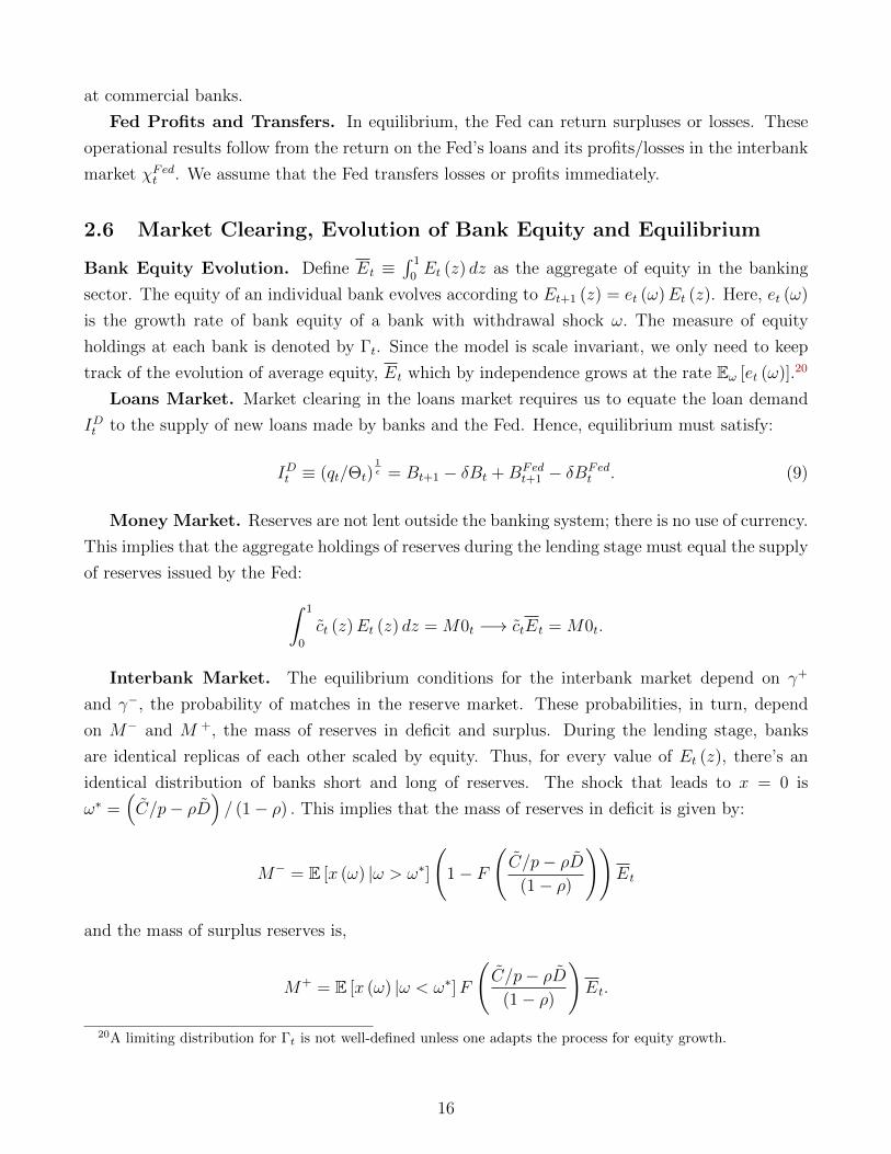
The left panel of Figure 2 shows the probability distribution of the reserve deficits during

the balancing stage, and the penalty associated with each deficit —the mass of the probability

30This value for the elasticity of loan-demand is consistent with the microfoundation provided in Appendix D,based on estimates of the elasticity of labor supply in the lower range.

31Since we consider a steady state without inflation, this is also the real interest rate.

26

distribution is rescaled to fit in the same plot. The penalty function χ has a kink at zero, because

rDW > rER. Notice that the distribution of the reserve deficits inherits the distribution of the

withdrawal shock, as the reserve deficit depends linearly on the withdrawal realization. Because

in equilibrium, there is an average excess surplus, the distribution’s mean is above zero.

The right panel of Figure 2 shows the distribution of equity growth as function ω. In equilib-

rium, banks that experience deposit inflows will increase their equity, whereas those that experience

outflows see their equity shrink. Because the penalty inflicts relatively higher losses to outflows

than to the benefits from inflows, the distribution of equity growth is skewed to the left. In par-

ticular, there is a fat tail with probabilities of losing about 2 percent of equity in a given period,

while the probability of growing more than 1 percent in a period is close to nil.

−2 −1 0 1 2−2

0

2

4

6 x 10−3

Position in Interbank Market

Withdrawal Risk (a)

x(γ+rFF + (1 − γ+)rER)

x(γ−rFF + (1 − γ−)rDW )

x

Prob

(

ω =(C + x)/DRd

− ρ)

(1 − ρ)

)

DeficitSurplus

−3 −2 −1 0 10

0.5

1

1.5

2

2.5

3

3.5 x 10−3Distribution of Equity Growth (b)

Equity Growth

Figure 2: Portfolio Choices and Effects of Withdrawal Shocks

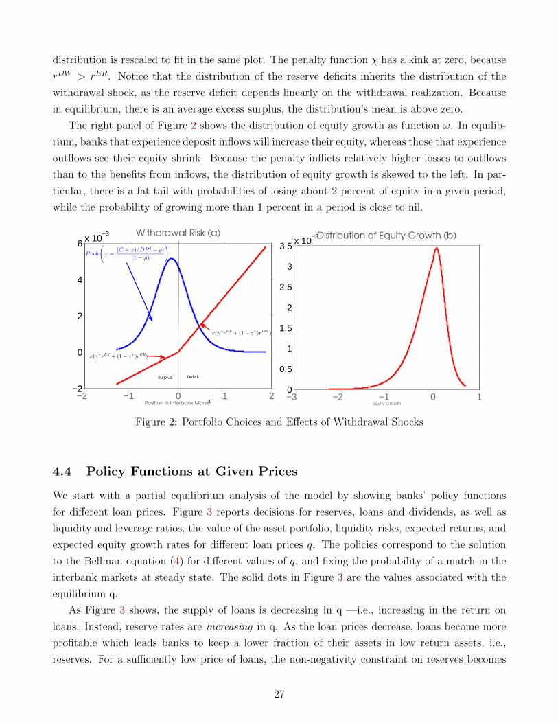
4.4 Policy Functions at Given Prices

We start with a partial equilibrium analysis of the model by showing banks’ policy functions

for different loan prices. Figure 3 reports decisions for reserves, loans and dividends, as well as

liquidity and leverage ratios, the value of the asset portfolio, liquidity risks, expected returns, and

expected equity growth rates for different loan prices q. The policies correspond to the solution

to the Bellman equation (4) for different values of q, and fixing the probability of a match in the

interbank markets at steady state. The solid dots in Figure 3 are the values associated with the

equilibrium q.

As Figure 3 shows, the supply of loans is decreasing in q —i.e., increasing in the return on

loans. Instead, reserve rates are increasing in q. As the loan prices decrease, loans become more

profitable which leads banks to keep a lower fraction of their assets in low return assets, i.e.,

reserves. For a sufficiently low price of loans, the non-negativity constraint on reserves becomes

27

0.9963 0.9971 0.9978 0.99850

0.2

0.4

0.6

0.8

1

1.2

1.4Cash-to-Equity Ratio

Loan Price (q)0.9963 0.9971 0.9978 0.9985

9.8

10

10.2

10.4

10.6

10.8

11

11.2Loan-to-Equity Ratio

Loan Price (q)0.9963 0.9971 0.9978 0.9985

0

0.005

0.01

0.015

0.02

0.025Dividends-to-Equity Ratio

Loan Price (q)

0.9963 0.9971 0.9978 0.9985

1.02

1.025

1.03

1.035

1.04Porfolio Value

Loan Price (q)0.9963 0.9971 0.9978 0.9985

0.99

1

1.01

1.02

1.03

1.04

1.05Mean Equity Growth

Loan Price (q)0.9963 0.9971 0.9978 0.9985

0

0.01

0.02

0.03

0.04

0.05

0.06

0.07

0.08

0.09

0.1Liquidity Ratio

Loan Price (q)

0.9963 0.9971 0.9978 0.998510

10

10

10

10

10

10

10Leverage

Loan Price (q)0.9963 0.9971 0.9978 0.9985

2

4

6

8

10

12

14

16Liquidity Risk

Loan Price (q)0.9963 0.9971 0.9978 0.9985

-6

-4

-2

0

2

4

6Excess Cash over Deposits

Loan Price (q)

Figure 3: Policy Function for Different Loan Prices

binding —banks only borrow reserves from the Fed and pay them back by the end of the balancing

stage.

In addition, dividends are increasing in q due to a substitution effect: when returns on loans

are high, banks cut dividend payments to allocate more funds to profitable lending. Exposure to

liquidity risk, measured as the standard deviation of the cost of rebalancing the portfolio χ(x)x,

is also decreasing in loan prices, reflecting the fact that banks’ asset portfolios become relatively

more illiquid when loan prices decrease.

28

5 Transitional Dynamics

This section studies the transitional dynamics of the economy in response to different shocks

associated with hypotheses 1–5. The shocks we consider are equity losses, a tightening of capital

requirements, an increase in the dispersion of withdrawals, a shutdown of the interbank market,

credit demand shocks, and changes in the discount window and interest rate on reserves. Shocks

are unanticipated upon arrival at t = 0 but their paths are deterministic for t > 0.32 Throughout

the experiments, we consider a monetary policy regime such that the Fed has a zero inflation

target RC = 0, i.e., the Fed performs open-market operations —altering MOt— to maintain price

stability: pt = p. 33

5.1 Equity Losses

We begin with a shock that translates into a sudden unexpected decline in bank equity. This shock

captures an unexpected rise in non-performing loans, security losses or off-balance sheet losses left

out of the model.34 Figure 4 illustrates how bank balance sheets shrink in response to 2 percent

equity losses. The top panel shows the evolution of total lending, total reserves, and liquidity risk,

and the bottom panel shows the level of equity, return on loans and the dividend rate.

To understand these dynamics, recall that all bank policy functions are linear in equity. Thus,

holding prices fixed, a loss in equity should lead to a proportional 2 percent decline in loans

and reserves. However, the contraction in loan supply also generates a drop in loan prices on

impact —through a movement along the loan demand. The reduction in q leads to an increase

in loan returns through the transition. As a consequence of the higher profitability on loans,

reserve holdings fall relatively more than loans. Banks shift their portfolios toward loans while

willingly exposing themselves to more liquidity risk. The overall return to the banks’s portfolio

also increases after the shock. With this, dividends fall as their opportunity cost increases. The

increase in bank returns and lower dividends leads to a gradual recovery of initial equity losses.

As equity recovers, the economy converges to the initial steady state and the transition is quick;

the effects of the shock cannot be observed after six quarters.

When δ > 0, there is an additional amplification effect not shown here. The reduction in the

supply of credit further lowers q, and this in turn, lowers marked-to-market equity, E, beyond the

initial impact of the shock. All other responses are therefore amplified.

32The assumption of unanticipated shocks is mainly for pedagogical purposes. In fact, it is relatively straight-forward to compute the model to allow for aggregate shocks, which are anticipated. Due to scale invariance, wewould not have to keep track of the cross-sectional distribution of equity anyway.

33We assume this not only for illustrative reasons but also because in the context of the Great Recession, thecore personal consumption expenditures index (PCE) remained close to 1 percent. It is straightforward to consideralternative monetary policy regimes.

34One way to incorporate this explicitly in the model would be to consider specific shocks to loan default rates.To the extent that equity is the only state variable, the analysis of the transitional dynamics is analogue to studyingthe evolution of the model under a richer structure for loans.

29

0 10 20-0.3

-0.2

-0.1

0

0.1Total Lending

0 10 20-30

-20

-10

0

10Total Cash

0 10 20-50

0

50

100

150

200Liquidity Risk

0 10 20-3

-2

-1

0

1Equity

0 10 20

0.8

1

1.2

1.4Return on Loans

0 10 200.0196

0.0198

0.02

0.0202Dividend Rate

Figure 4: Impulse Response to Equity Losses

5.2 Capital Requirements

The effects of a sudden and transitory tightening of capital requirements, i.e., a reduction in κ, are

shown in Figure 5. The shock is a 10 percent decrease in κ which is associated with a 1 percent

increase in the capital ratio of banks for the calibrated level of leverage.

The short-run behavior of the transition is very similar to the behavior after equity losses. As

with equity losses, the contraction in capital requirements reduces the supply of loans because as

the constraint gets tighter, banks must operate as if they had less equity—the capital requirement

is binding in the steady state.

In the medium term, equity begins to exceed its steady state value. This happens because

the return on loans increases and banks pay less dividends. Eventually, the increase in equity

overcomes the increase in capital requirements. Ultimately, the economy converges back to a

steady state level of equity as the capital requirement shock converges back to its original level.

30

0 10 20-0.6

-0.4

-0.2

0

0.2Total Lending

0 10 20-80

-60

-40

-20

0

20Total Cash

0 10 20-200

0

200

400

600Liquidity Risk

0 10 20-1

0

1

2

3

4Equity

0 10 200.5

1

1.5

2

2.5Return on Loans

0 10 200.0198

0.02

0.0202

0.0204

0.0206Dividend Rate

Figure 5: Impulse Response to a Tightening in Capital Requirements

5.3 Interbank Market Shocks

5.3.1 Bank-Run Shocks

Here we study the possibility of a bank run. We consider a 5 percent probability that all the

deposits are withdrawn from a given bank —that is ω = 1. This bank runs are on individual

institutions as we maintain the assumption that deposits are not withdrawn from the banking

system as a whole.35 We assume that this bank run probability follows a deterministic AR(1)

process such that the shock lives for about two years. The effects of this shock are illustrated in

Figure 6.

The risk of a bank run generates an increase in liquidity risk, leading banks to hoard reserves.

Because reserve requirements are constant, this means that banks accumulate more excess reserves.

Notice that the liquidity risk is still about three times larger than in the steady state although

banks hold more reserves. As the Fed’s objective is a zero inflation target, the Fed supplies reserves

to meet this target. Naturally, higher liquidity costs induce a decline in the supply of loans, as

banks substitute loans for reserves. In equilibrium, this leads to an increase in the price of loans

and a decline in the aggregate volume of lending.

In tandem, banks respond to the risk of a bank run by cutting dividend payments. Although

35Thus we adjust F accordingly by assuming a 5 percent probability of a large inflow of deposits. It is alsopossible to extend the model to study system-wide bank runs, as in Uhlig (2010) (see also Robatto (2013)).

31

0 10 20-0.06

-0.04

-0.02

0

0.02Total Lending

0 10 20-2

0

2

4

6

8Total Cash

0 10 20-100

0

100

200

300Liquidity Risk

0 10 20-0.2

0

0.2

0.4

0.6Equity

0 10 200.75

0.8

0.85

0.9

0.95Return on Loans

0 10 200.02

0.02

0.02

0.02

0.0201

0.0201Dividend Rate

Figure 6: Impulse Response to a Bank-Run Shock

higher liquidity costs are associated with lower returns, the contraction in loan supply generates

a more-than-compensating increase in expected bank returns. This leads to an increase in equity

over time. As equity grows, this mitigates the fall in lending ratios. Eventually, lending rises

above its steady state value. This is because several quarters after the shock is realized, the effect

on bank equity compensates for the portfolio effect, as the shock begins to decay.

5.3.2 Interbank Market Shutdown

Disruptions in the interbank market can be studied through shocks that drive the probability of

a match in the interbank market to zero.36 Hence, reserves are borrowed (lent) only from (to)

the Fed. In particular, banks that face a reserve deficit borrow directly at rDW . Thus, this shock

increases expected liquidity costs. The effects of the interbank market freeze are shown in Figure

7. Overall, the effects are similar to the bank run shock we describe earlier.

36A recent macroeconomic model of endogenous interbank market freezing due to asymmetric information withone-period lived banks is Boissay et al. (2013).

32

0 10 20-0.04

-0.03

-0.02

-0.01

0

0.01Total Lending

0 10 20-1

0

1

2

3Total Cash

0 10 20-50

0

50

100

150Liquidity Risk

0 10 20-0.05

0

0.05

0.1

0.15Equity

0 10 200.75

0.8

0.85

0.9

0.95Return on Loans

0 10 200.02

0.02

0.02

0.02

0.02Dividend Rate

Figure 7: Impulse Response to Freezing in Interbank Markets

5.4 Credit Demand

The effects of negative credit demand shocks are captured through a decline in Θt. Figure 8 illus-

trates the effects of a negative temporary shock to Θt. We assume the shock follows a deterministic

AR(1) process that lasts for about seven years.

The effects of credit demand shocks contrast sharply with the effect of the shocks considered

above, because all of the prior shocks cause a contraction in the supply of loans. In contrast,

demand shocks cause a decline in the return on loans —and a shift along the supply curve. As a

result, banks shift their portfolios toward reserves —as the opportunity cost of holding reserves

lowers. The liquidity risk almost vanishes. Initially, banks respond by paying higher dividends

due to the overall decline in the their portfolio returns. The reduction in returns and dividend

increments brings equity below the steady state. As the shock decays —around a year and a half

later— the economy follows a similar transition as with the shock to equity, slowly increasing

lending rates and reducing dividend rates until equity returns to the steady state.

33

0 10 20-10

-5

0

5Total Lending

0 10 20-50

0

50

100

150Total Cash

0 10 20-100

-50

0

50

100Liquidity Risk

0 10 20-5

-4

-3

-2

-1

0Equity

0 10 200

0.5

1

1.5Return on Loans

0 10 200.019

0.0195

0.02

0.0205

0.021Dividend Rate

Figure 8: Impulse Response to Credit Demand Shock

5.5 Policy Rates

5.5.1 Discount Window

We now analyze the effects of interest rate policy shocks. In the experiment, we study a positive

shock of 100 basis points (bps) to the discount window rate, expressed at annualized rates. The

effects of an increase in the discount window rate are depicted in Figure 9. Banks respond to

this increase by reducing lending. Policy effects are similar to the effects of shocks that increase

liquidity costs. Notice that the pass-through from the policy rate to the return on loans is almost

perfect.

5.5.2 Interest on Reserves

A shock to the interest on excess reserves works similarly to an increase in the discount window rate

since both increase the return of holding reserves. We study a shock that raises this rate from 0 bps

to 100bps (annualized), a shock that corresponds to the recent Fed policy of remunerating excess

reserves. The effect of this policy is illustrated in Figure 10. The shock makes reserves relatively

more attractive. In response, banks reallocate their portfolio from loans toward reserves.37

37Notice that liquidity risk does not decline despite the increase in cash holdings by banks. This occurs becausethe increase in the interest rate on excess reserves leads to larger differences in returns between banks on surplusand banks on deficit.

34

0 10 20-0.15

-0.1

-0.05

0

0.05Total Lending

0 10 20-5

0

5

10

15Total Cash

0 10 20-20

0

20

40

60

80Liquidity Risk

0 10 20-0.2

0

0.2

0.4

0.6

0.8Equity

0 10 200.7

0.8

0.9

1

1.1Return on Loans

0 10 200.0199

0.02

0.02

0.0201

0.0201Dividend Rate

Figure 9: Impulse Response to a Rise in the Discount Window Rate

0 10 20-0.03

-0.02

-0.01

0

0.01Total Lending

0 10 20-1

0

1

2

3

4Total Cash

0 10 20-5

0

5

10

15Liquidity Risk

0 10 20-0.05

0

0.05

0.1

0.15

0.2Equity

0 10 200.76

0.78

0.8

0.82

0.84

0.86Return on Loans

0 10 200.02

0.02

0.02

0.02

0.0201

0.0201Dividend Rate

Figure 10: Impulse Response to a Shock to the Interest Rate on Excess Reserves

35

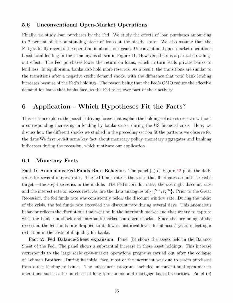
5.6 Unconventional Open-Market Operations

Finally, we study loan purchases by the Fed. We study the effects of loan purchases amounting

to 2 percent of the outstanding stock of loans at the steady state. We also assume that the

Fed gradually reverses the operation in about four years. Unconventional open-market operations

boost total lending in the economy, as shown in Figure 11. However, there is a partial crowding-

out effect. The Fed purchases lower the return on loans, which in turn leads private banks to

lend less. In equilibrium, banks also hold more reserves. As a result, the transitions are similar to

the transitions after a negative credit demand shock, with the difference that total bank lending

increases because of the Fed’s holdings. The reason being that the Fed’s OMO reduce the effective

demand for loans that banks face, as the Fed takes over part of their activity.

6 Application - Which Hypotheses Fit the Facts?

This section explores the possible driving forces that explain the holdings of excess reserves without

a corresponding increasing in lending by banks sector during the US financial crisis. Here, we

discuss how the different shocks we studied in the preceding section fit the patterns we observe for

the data.We first revisit some key fact about monetary policy, monetary aggregates and banking

indicators during the recession, which motivate our application.

6.1 Monetary Facts

Fact 1: Anomalous Fed-Funds Rate Behavior. The panel (a) of Figure 12 plots the daily

series for several interest rates. The fed funds rate is the series that fluctuates around the Fed’s

target —the step-like series in the middle. The Fed’s corridor rates, the overnight discount rate

and the interest rate on excess reserves, are the data analogues ofrDWt , rERt

. Prior to the Great

Recession, the fed funds rate was consistently below the discount window rate. During the midst

of the crisis, the fed funds rate exceeded the discount rate during several days. This anomalous

behavior reflects the disruptions that went on in the interbank market and that we try to capture

with the bank run shock and interbank market shutdown shocks. Since the beginning of the

recession, the fed funds rate dropped to its lowest historical levels for almost 5 years reflecting a

reduction in the costs of illiquidity for banks.

Fact 2: Fed Balance-Sheet expansion. Panel (b) shows the assets held in the Balance

Sheet of the Fed. The panel shows a substantial increase in these asset holdings. This increase

corresponds to the large scale open-market operations programs carried out after the collapse

of Lehman Brothers. During its initial face, most of the increment was due to assets purchases

from direct lending to banks. The subsequent programs included unconventional open-market

operations such as the purchase of long-term bonds and mortgage-backed securities. Panel (c)

36

0 10 20-2

-1.5

-1

-0.5

0

0.5Total Lending

Bank LendingTotal Loans

0 10 20-10

0

10

20

30Total Cash

0 10 20-60

-40

-20

0

20Liquidity Risk

0 10 20-1.5

-1

-0.5

0Equity

0 10 200.4

0.5

0.6

0.7

0.8

0.9Return on Loans

0 10 200.0194

0.0196

0.0198

0.02

0.0202Dividend Rate

Figure 11: Impulse Response to Unconventional Monetary Policy

shows the increase in the Fed’s assets from direct lending to banks and mortgage-backed securities

—liquidity facilities and MBS, see the data Appendix for more details. The series is reported in

terms relative to the total of bank credit of US commercial banks. Whereas prior to the crisis, this

figure was close to 0 percent, this ratio reached 18 percent by the middle of 2014. The counterpart

of this figure is a proportional increase in Fed’s liabilities, reserves. The model captures these

open-market operations through the Fed’s purchases of loans.

Fact 3: Excess-Reserve Holdings. Panel (d) shows an increment in holdings of excess

reserves by the banking system. Whereas prior to the crisis there were virtually no excess reserves,

during its aftermath, excess reserves amount almost 16 times greater than the amount of required

reserves.

Fact 4: Depressed Lending Activities. Panel (e) shows the decline in commercial and

industrial (C&I) lending during the crisis. The figure shows the raw series and a series that

subtracts the decline in the stock of C&I loan commitments from the original series. This figure

shows that while there was a large monetary expansion by the Fed during the middle of the crisis,

there was a simultaneous substantial decline in lending to firms.

Fact 5: Drop in Money Multiplier. The large drop in the money multiplier for M1 is a

summarizes facts 2, 3, and 4. This is shown in Panel (f).

37

Figure 12: Monetary Facts

38

6.2 Banking Facts

Our model yields predictions about the behavior of several banking indicators for different shocks.

We will use this information to gain further insights about the nature of the shocks that affected

banks during the crisis. Here, we report four indicators computed from Commercial Bank Call

Reports. These ratios are reported as simple averages and averages weighted by assets for the

cross-section at a given point in time. We summarize the main facts we want to underscore:

Fact 6: Decline in Book-Value Leverage. The upper-left panel of Figure 13 shows the

decline in the tangible leverage —a meausure that subtracts tangible assets from the book value

of equity. From its peak at the middle of the crisis to 2010Q4, the average tangible leverage falls

from 16 to about 12.

Fact 7: Increase Liquidity Ratio. The upper-right panel of Figure 13 shows the behavior

of the liquidity ratio, the ratio of liquid assets over total assets. Here we take liquid assets to be the

sum of reserves plus Treasury bills. The data shows an increase from 6 percent to 12 percent for

the same period. Interestingly, this implies the increase in reserves was not offset by the reduction

in other liquid assets.

Fact 8: Bank-Equity Losses. The bottom-left panel of Figure 13 shows the behavior of

the realized returns on equity. The figure shows a sharp decline that begins in 2007Q4 from its

historical average to a value of about 0. By the middle of the crisis, we observe an even further

decline, especially concentrated among the largest banks. During the peak of the crisis, losses

exceeded 5 percent on average and almost reach 10 percent for the average weighted by assets.

Fact 9: Dividends. The bottom-right panel of Figure 13 plots the evolution of the dividend-

per-equity of banks. Dividends already showed a declining trend prior to the Great Recession. This

further declines all throughout the duration of the recession, but erratically increases thereafter.

Although the model also yields predictions for the dividend yield in the model, it is worth noting

that dividends were also constrained by policy during the crisis.

The following section discusses which combination of shocks —and hypothesis— are more

consistent with the banking and monetary facts we have described so far.

39

Figure 13: Banking Indicators: The figure reports four indicators of banking activity for the universe of commercial banks in theUS. All the series correspond to ratios of variables reported by computing simple averages and averages weighted by assets. Tangibleleverage in (a) is total liabilities relative to equity minus intangible assets. The liquidity ratio in (b) is the sum of vault cash, reserves,and Treasury securities relative to total assets. The return on equity in (c) is the ratio of net operating revenues over equity. Thedividend ratio in (d) is the sum of common and preferred dividends over equity. More details are found in Appendix E.

40

6.3 Which Hypotheses Fit the Facts?

We can now use our model as a laboratory to investigate how important are hypothesis 1–5 in

explaining the facts described above. In particular, we can shed light on what are the possible

drivers of the increase in liquidity and the persistent drop in lending that occurred in October 2008

after the failure of Lehman Brothers. We first describe the qualitative prediction of our model

and then turn to a quantitative evaluation

6.3.1 Discussion

The shocks that we study can be classified into supply and demand shocks. Within supply shocks,

we have two classes of shocks. First, equity losses and increments in capital requirements constrain

the entire portfolio of the bank. As analyzed above, by reducing the supply of loans and raising the

relative return on loans relative to reserves, banks substitute reserves for lending. Hence, these two

hypotheses can explain the collapse in lending but are inconsistent with the observed increase in

liquidity ratios by banks. Second, we have shocks to higher uncertainty in the withdrawal process

Ft, the shutdown of the interbank market, and the increase in corridor rates. These shocks do

not affect on impact the funding capacity of the bank but reduce the relative return on loans.

As a result, banks substitute lending for reserves, and in addition, pay less dividends, which is

consistent with the pattern that we see in the midst of the crisis. However, as of 2010 more flexible

lending facilities by the Fed, probably reduce the importance of these supply shocks. In fact, a

reduction of the discount window rate in our model, as observed since 2009, significantly reduce

the quantitative importance of shocks leading to either higher uncertainty or higher disruptions in

interbank markets. Finally, interest on reserves also deliver effects consistent with the data, but

it has quantitatively mild effects.

With regards to demand shocks, a negative credit demand shock reduces return on loans and

leads banks to substitute reserves for lending. Therefore, this shock is consistent with the decline

in bank lending and the increase in reserves holdings —through a substitution effect. This shock

is, however, inconsistent with the path for dividends that were sharply reduced at the beginning

of the crisis.38 Finally, the low lending rates of 2010 also favors the hypothesis of a persistent

negative credit demand shock.39

To summarize, the model supports hypothesis 3 associated with disruptions in the interbank

markets and hypothesis 5 associated with a persistent negative credit demand shock. The short-

run effects after each shock are summarized by the arrows in the table below.

38The path for dividends was also influenced by government policies, in particular for those financial institutionsthat participated in government recapitalization programs.

39Some caution also has to be taken from using low lending rates as evidence for credit demand shocks for at leasttwo reasons. First, there is a change in the composition of credit towards less risky loans. Second, besides interestrates, banks seem to have tightening lending standards, e.g. by requiring higher downpayments in mortgages.

41

Table 2: Summary of Effects on Impact

Loans Cash Div. Equity

Equity Loss ↓ ↓ ↓ ↓

Capital Requirement ↓ ↓ ↓ ↑

Uncertainty ↓ ↑ ↓ ↑

Credit Demand ↓ ↑ ↑ ↓

Interest on Reserves ↓ ↑ ↓ ↑

Data ↓ ↑ ↓ ↓

6.3.2 Quantitative Evaluation

The goal of this section is to assess the model’s ability to quantitatively account for the monetary

and banking facts we described in the previous section. For this purpose, we compute the model’s

transitional dynamics after a sequences of deterministic shocks assuming the economy was in

steady state in 2007.Q3. In this experiment, we feed in a sequence of supply shocks that we

interpret as observables and impute demand shocks as a residual to match the decline in lending.

Shocks. We feed the following shocks, in line with the hypothesis discussed above. First, we

consider a shock to bank equity losses of 2 percent, which is equivalent to 0.2 percent of total assets

—this shock assumes a corresponding decline in loans keeping liabilities constant. The magnitude

of this shock corresponds to the unexpected losses of AAA-rated subprime MBS tranches, esti-

mated by Park (2011). Second, we consider a shock that anticipates higher capital requirements

along the new prescriptions of Basel III. In particular, we assume that agents anticipate that the

maximum leverage ratio will be permanently reduced from κ = 15 to κ = 12 starting 2013.Q1.

This is in line with new regulations that require a gradual increase in capital requirements of 2

percent between 2013.Q1 and 2015.Q4 (see BIS (2010)). Third, we consider a freezing of interbank

market during 2008.Q3 and 2008.Q4, in line with the evidence of a sharp decrease in the Fed funds

market and the increase in discount window operations which reached 400 billion dollars at the

peak of the crisis.40 As explained above, this implies the probability of a match in the interbank

markets in the balancing stage becomes zero, so that banks only trade with the Fed.

The two remaining observable shocks we consider are policy responses by the Fed. First, we

feed the sequence for discount window rates and interest on excess reserves shown in panel (a) of

Figure ?? . We also assume that these policies reverse gradually to steady state starting in 2015.

40The amount of Fed funds sold was reduced by a factor of 4 in 2008Q3, and never recover from pre-crisis levels.We consider only two periods for this shock because as described in Section 6.1, interbank market rates normalizedfollowing various policies by the Fed. Moreover, because discount window rates were significantly reduced in2009.Q3, results would be very similar with more persistent shocks.

42

Second, we feed the sequence of loan purchases as part of the unconventional OMO carried out by

the FED, as described in Fact 2. We assume that these operations are gradually reversed starting

in 2020, except for the interest on reserves that we assume they stay at a constant level of 0.2

percent (annualized).

Finally, we estimate a credit demand shock. Given the observed time series for loans shown

in Figure ??, we consider a a shock to Θt to match the decline in lending. Specifically, Θ−1t is

reduced by about 1.1 percent in every quarter from 2008.Q3 to 2010.Q4 and stays permanently

at a level of 12 percent below the steady state.

Results. Figures ??-?? show the evolution of loans, liquidity ratios, dividend rates and the

return on loans in the data and in the model for different simulation scenarios.41 Figure ?? shows

that the model that includes all shocks can account reasonably well for the key patterns in the

data. As it turns out, the credit demand shock is the most important one. To see this, consider

the third panel from Figure ?? which feeds all shocks considered except for the credit demand

shock.

Notice also that the money multiplier is also falling, ...

2007.Q4 2008.Q4 2009.Q4 2010.Q4 -15

-10

-5

0

5Total Lending

2007.Q4 2008.Q4 2009.Q4 2010.Q4 0.04

0.06

0.08

0.1

0.12Liquidity Ratio

2007.Q4 2008.Q4 2009.Q4 2010.Q4 0

2

4

6

8

10Dividend Ratio

2007.Q4 2008.Q4 2009.Q4 2010.Q4 1

2

3

4

5Rate on Loans

2007.Q4 2008.Q4 2009.Q4 2010.Q4 -12

-10

-8

-6

-4

-2

0Total Lending

2007.Q4 2008.Q4 2009.Q4 2010.Q4 0

0.05

0.1

0.15

0.2Liquidity Ratio

2007.Q4 2008.Q4 2009.Q4 2010.Q4 7.4

7.6

7.8

8

8.2

8.4Div. Rate (annual %)

2007.Q4 2008.Q4 2009.Q4 2010.Q4 0

0.5

1

1.5

2Rate on Loans

Figure 14: All Shocks

41For the model simulations, variations in lending are taken with respect to the steady state. For the data, thepercentage change in lending takes September 2007 as the basis value. Return on loans in the data correspond tothe real return on one-year mortgage rates.

43

7 Conclusions

Modern monetary-macro models have developed independently from banking models. Recent

crises in the US, Europe and Japan, however, have revealed the need of a model to study monetary

policy in conjunction with the banking system. This model should be used as a tool to address

many issues that emerge in current policy debates.

This paper presents a dynamic macro model to study the implementation of monetary policy

through the liquidity management of banks. We used the model to understand the effects of

various shocks to the banking system. As an application, we employ the model to contribute

to one policy question: why have banks held on to so many reserves and not expanded their

lending? We argued that an early interbank market freeze may have been important at an the

early beginning of the Great Recession. However, a persistent decline in the demand for loans

seems the most plausible story to explain the increase in the holding of reserves and the decline in

lending since 2008 onwards. This result is suggestive of phenomena where an initial contraction

in the loans supply eventually translates into a subsequent strong and permanent contraction in

demand for credit.

We believe the model can be used to answer a number of other issues present in policy debates.

For example, the model can be used to study the Fed’s exit strategy and the fiscal implications. In

addition, it can also be used to analyze changes in policy tools used in monetary policy implemen-

tation in the past. There are also other possible relevant extensions of the model. An extension

that breaks aggregation may allow to study the cross-sectional responses of banks depending their

liquidity and leverage ratios. Introducing aggregate shocks would also allow us to investigate the

role of liquidity requirements and capital requirements as macroprudential tools. We hope that

the model we propose can be useful for policy analysis.

44

References

Afonso, Gara and Ricardo Lagos, “Trade Dynamics in the Market for Federal Funds,” 2012.

Mimeo, NY Fed. 5, 8

Allen, Franklin and Douglas Gale, “Optimal Financial Crises,” The Journal of Finance, 1998,

53 (4), 1245–1284. 5

Alvarez, Fernando and Nancy L Stokey, “Dynamic Programming with Homogeneous Func-

tions,” Journal of Economic Theory, 1998, 82 (1), 167 – 189. 12, 53

Armantier, Olivier, Eric Ghysels, Asani Sarkar, and Jeffrey Shrader, “Stigma in financial

markets: Evidence from liquidity auctions and discount window borrowing during the crisis,”

2011. FRB of New York Staff Report. 8

Atkeson, Andrew G, Andrea L Eisfeldt, and Pierre-Olivier Weill, “The market for otc

credit derivatives,” 2012. Working Paper, UCLA. 8

Bagehot, Walter, Lombard Street: A description of the money market, Wiley, 1873. 4

Bassett, William F, Mary Beth Chosak, John C Driscoll, and Egon Zakrajsek, “Identi-

fying the macroeconomic effects of bank lending supply shocks,” 2010. Mimeo, Federal Reserve

Board. 26

Bernanke, Ben S. and Alan S. Blinder, “Credit, Money, and Aggregate Demand,” The

American Economic Review, 1988, 78 (2), pp. 435–439. 4

Bigio, Saki, “Financial Risk Capacity,” 2010. 21

, “Endogenous liquidity and the business cycle,” 2011. Mimeo, New York University. 60

and Jeremy Majerovitz, “A Guide to the using Bank Data from the Call Reports,” 2013.

63

BIS, “Basel III: A global regulatory framework for more resilient banks and banking systems,”

2010. Basel Committee on Banking Supervision, Basel. 42

Boissay, Frederic, Fabrice Collard, and Frank Smets, “Booms and systemic banking crises,”

2013. Mimeo, European Central Bank. 32

Bolton, Patrick and Xavier Freixas, “Corporate Finance and the Monetary Transmission

Mechanism,” The Review of Financial Studies, 2009, 19 (3), 829–870. 6

Brunnermeier, Markus K. and Yuliy Sannikov, “The I-Theory of Money,” 2012. Mimeo,

Princeton. 5

45

Buera, Francisco and Juan Pablo Nicolini, “Liquidity Traps and Monetary Policy: Managing

a Credit Crunch,” 2013. Mimeo, Chicago Fed. 23

Cavalcanti, Ricardo, Andres Erosa, and Ted Temzelides, “Private Money and Reserve

Management in a Random Matching Model,” Journal of Political Economy, 1999, 107 (5), pp.

929–945. 5

Chodorow-Reich, Gabriel, “The Employment Effects of Credit Market Disruptions: Firm-level

Evidence from the 2008–9 Financial Crisis,” The Quarterly Journal of Economics, 2014, 129

(1), 1–59.

Christiano, Lawrence J. and Martin Eichenbaum, “Liquidity Effects and the Monetary

Transmission Mechanism,” The American Economic Review, 1992, 82 (2), pp. 346–353. 59, 60

Corbae, Dean and Pablo D’Erasmo, “A Quantitative Model of Banking Industry Dynamics,”

2013. Mimeo, Wisconsin. 13

and , “Capital Requirements in a Quantitative Model of Banking Industry Dynamics,” 2014.

13

Curdia, Vasco and Michael Woodford, “Conventional and Unconventional Monetary Policy,”

2009. Mimeo, NY Fed. 4

den Haan, Wouter J., Steven W. Sumner, and Guy Yamashiro, “Construction of Aggre-

gate and Regional Bank Data Using the Call Reports,” 2002. 63

Diamond, Douglas W., “Financial Intermediation and Delegated Monitoring,” The Review of

Economic Studies, 1984, 51 (3), pp. 393–414. 6

Diamond, Douglass W. and Phillip H. Dybvig, “Bank runs, deposit insurance, and liquid-

ity,” Journal of Political Economy, 1983, 91 (3), 401–419. 5

Duttweiler, Rudolf, Managing Liquidity in Banks: A Top Down Approach, John Wiley & Sons

Ltd, 2009. 5

Ennis, Huberto M and John A Weinberg, “Over-the-counter loans, adverse selection, and

stigma in the interbank market,” Review of Economic Dynamics, 2013, 16 (4), 601–616. 8

and Todd Keister, “Bank runs and institutions: The perils of intervention,” The American

Economic Review, 2009, 99 (4), 1588–1607. 5

Frost, Peter A., “Banks’ Demand for Excess Reserves,” Journal of Political Economy, 1971, 79

(4), pp. 805–825. 4

46

Gertler, Mark and Nobuhiro Kiyotaki, “Banking, Liquidity and Bank Runs in an Infinite

Horizon Economy,” 2013. Mimeo, NYU. 5

and Peter Karadi, “A Model of Unconventional Monetary Policy,” Journal of Monetary

Economics, 2009. 4

Gurley, John G. and Edward S. Shaw, Money in a Theory of Finance 1964. 4

Holmstrm, Bengt and Jean Tirole, “Private and Public Supply of Liquidity,” The Journal of

Political Economy, 1998, 106 (1), pp. 1–40. 5

Holmstrom, Bengt and Jean Tirole, “Financial Intermediation, Loanable Funds, and the

Real Sector,” The Quarterly Journal of Economics, 1997, 112 (3), pp. 663–691. 6

Jimenez, Gabriel, Steven Ongena, Jose-Luis Peydro, and Jesus Saurina, “Credit Supply

and Monetary Policy: Identifying the Bank Balance-Sheet Channel with Loan Applications,”

The American Economic Review, 2012, 102 (5), pp. 2301–2326. 5

Jimnez, Gabriel, Steven Ongena, Jos-Luis Peydr, and Jess Saurina, “Hazardous Times

for Monetary Policy: What do 23 Million Loans Say About the Impact of Monetary Policy on

Credit Risk-Taking?,” 2014. forthcoming in Econometrica. 5

Kashyap, Anil and Jeremy Stein, “What Do a Million Observations on Banks Say About the

Transmission of Monetary Policy?,” American Economic Review, June 2000, 90 (3), 407–428.

5, 63

Leland, Hayne E. and Klaus Bjerre Toft, “Optimal Capital Structure, Endogenous

Bankruptcy, and the Term Structure of Credit Spreads,” The Journal of Finance, 1996, 51

(3), pp. 987–1019. 6

Mishkin, Frederic S., “Over the Cliff: From the Subprime to the Global Financial Crisis,” The

Journal of Economic Perspectives, 2011, 25 (1), pp. 49–70. 4

Park, Sunyoung, “The Size of the Subprime Shock,” 2011. Korea Advanced Institute of Science

and Technology, working paper. 42

Poole, William, “Commercial Bank Reserve Management in a Stochastic Model: Implications

for Monetary Policy,” The Journal of Finance, 1968, 23 (5), pp. 769–791. 4

Robatto, Roberto, “Financial Crises and Systemic Bank Runs in a Dynamic Model of Banking,”

2013. Mimeo, University of Chicago. 31

Saunders, Anthony and Marcia Cornett, Financial Institutions Management: A Risk Man-

agement Approach, McGraw-Hill/Irwin Series in Finance, Insurance and Real Estate, 2010. 5

47

Stein, Jeremy C., “Monetary Policy as Financial Stability Regulation,” The Quarterly Journal

of Economics, 2012, 127 (1), pp. 57–95. 5

Stein, Jeremy, Robin Greenwood, and Samuel Hanson, “A Comparative-Advantage Ap-

proach to Government Debt Maturity,” 2013. Mimeo, Harvard. 5

Uhlig, Harald, “A model of a systemic bank run,” Journal of Monetary Economics, 2010, 57

(1), 78–96. 31

Williamson, Stephen, “Costly Monitoring, Loan Contracts, and Equilibrium Credit Rationing,”

The Quarterly Journal of Economics, 1987, 102 (1), pp. 135–146. 6

, “Liquidity, Monetary Policy, and the Financial Crisis: A New Monetarist Approach,” 2012.

forthcoming, American Economic Review, 2012. 5

and Randall Wright, “New monetarist economics: Models,” Handbook of Monetary Eco-

nomics, 2010, 3, 25–96. 5

Wolman, Alexander and Huberto Ennis, “Large Excess Reserves in the US: A View from

the Cross-Section of Banks,” 2011. Federal Reserve Bank of Richmond, Manuscript. 13

Woodford, Michael, “Financial Intermediation and Macroeconomic Analysis,” The Journal of

Economic Perspectives, 2010, 24 (4), 21–44. 4

48

A Proofs

A.1 Proof of Propositions 1, 2 and 3

This section provides a proof of the optimal policies described in Section 3.4. The proof of

Proposition 1 is straightforward by noticing that once E is determined, the banker does not care

how he came up with those resources. The proof of Propositions 2 and 3 is presented jointly

and the strategy is guess and verify. Let X be the aggregate state. We guess the following.

V (E;X) = v (X)E1−γ where v (X) is the slope of the value function, a function of the aggregate

state that will be solved for implicitly. Policy functions are given by: DIV (E;X) = div (X)E,

B (E;X) = b (X)E, D (E;X) = d (X)E and C (X) = c (X)E, for div (X) , b (X) , d (X) and

c (X) policy functions that are independent of E.

A.1.1 Proof of Proposition 2

Given the conjecture for functional form of the value function, the value function satisfies:

V (E;X) = maxDIV,C,B,D∈R

U(DIV ) + βE[v (X ′) (E ′)

1−γ)|X]

Budget Constraint: E = qB + Cp+DIV − D

RD

Evolution of Equity : E ′ = (q′δ + (1− δ)) B + Cp′ − D − χ

((ρ+ ω′ (1− ρ))

D

RD− pC

)

Capital Requirement :D

RD≤ κ

(Bq + Cp− D

RD

)

where the form of the continuation value follows from our guess. We can express all of the

constraints in the problem as linear constraints in the ratios of E. Dividing all of the constraints

by E, we obtain:

1 = div + qb+ pc− d

Rd

E ′/E = (q′δ + 1− δ) b+ cp′ − d− χ((ρ+ ω′ (1− ρ))D − pC)

d

RD≤ κ(bq + cp− d

RD)

where div = DIV/E,b = B/E, c = C/E and d = D/E. Since, E is given at the time of the

decisions of B,C,D and DIV , we can express the value function in terms of choice of these ratios.

49

Substituting the evolution of E ′ into the objective function, we obtain:

V (E;X) = maxwb,wc,wd,div∈

U(divE) + βE[v (X ′) (R (ω,X,X ′)E)

1−γ)|X]

1 = div + qb+ pc− dd

RD≤ κ

(bq + cp− d

RD

)

where we use the fact that E ′ can be written as:

E ′ = R (ω′, X,X ′)E

where R (ω′, X,X ′) is the realized return to the bank’s equity and defined by:

R (ω′, X,X ′) ≡ (q (X ′) δ + (1− δ)) b+ p (X ′) c− d− χ((ρ+ ω′ (1− ρ))d

RD− p (X) c).

We can do this factorization for E because the evolution of equity on hand is linear in all the

term where prices appear. Moreover, it is also linear in the penalty χ also. To see this, observe

that χ(

(ρ+ ω′ (1− ρ)) DRD− pC

)= χ

((ρ+ ω′ (1− ρ)) dE

RD− cE

)by definition of

d, c. Since,

E ≥ 0 always, we have that

(ρ+ ω′ (1− ρ))D

RD− C ≤ 0↔

((ρ+ ω′ (1− ρ))

d

RD− c

)≤ 0.

Thus, by definition of χ,

χ((ρ+ ω′ (1− ρ))D

RD− C) =

Eχ(

(ρ+ ω′ (1− ρ)) dRD− c)

if(

(ρ+ ω′ (1− ρ)) dRD− c)≤ 0

Eχ(

(ρ+ ω′ (1− ρ)) dRD− c)

if(

(ρ+ ω′ (1− ρ)) dRD− c)> 0

.

= Eχ(

(ρ+ ω′ (1− ρ))d− c).

Hence, the evolution of R (ω′, X,X ′) is a function of the portfolio ratios b, c and d but not of

the level of E. With these properties, we can factor out, E1−γ from the objective because it is a

constant when decisions are made. Thus, the value function may be written as:

V (E;X) = E1−γ[

maxwb,wc,wd,div∈

U(div) + βE[v (X ′)R (ω,X,X ′)

1−γ)|X]]

(14)

1 = div + qb+ pc− d

d ≤ κ(Bq + Cp− d) (15)

50

Then, let an arbitrary v (X) be the solution to:

v (X) = maxwb,wc,wd,div∈

U(div) + βE[v (X ′)R (ω,X,X ′)

1−γ)|X]

1 = div + qb+ pc− d

RD

d

RD≤ κ(bq + cp− d

RD)

We now show that if v (X) exists, v (X) = v (X) verifies the guess to our Bellman equation. Sub-

stituting v (X) for the particular choice of v (X) in (14) allows us to write V (E;X) = v (X)E1−γ.

Note this is true because maximizing over div, c, b, d yields a value of v (X) . Since, this also shows

that div, c, b, d and independent of E, and DIV = divE, B = bE, C = cE and D = dE.

A.1.2 Proof of Proposition 3

We have from Proposition 2 that

v(X) = maxwb,wc,wd,div4+

U(div) + βE [v (X ′) |X] .....

Eω′(

(q′δ + (1− δ))b+ p′c− d− χ((ρ+ ω′ (1− ρ)) d/RD − pc))1−γ

subject to

1 = qb+ pc+ div − d

RD

d

RD≤ κ

(qb+ cp− d

RD

)

Now define:

wb ≡bq

(1− div), wc ≡

cp

(1− div)and wd ≡

d

RD (1− div).

and collecting terms on 1 = qb+ pc+ div − dRD, we obtain:

div + (1− div) (wb + wc + wd) = 1⇔ .wb + wc − wd = 1

51

Then using the definition of wb, wc, wd have that v (X)

v (X) = maxwb,wc,wd,div∈R4

+

U(div) + βE [v (X ′) |X] (1− div)1−γ...

Eω′q′δ + (1− δ)

qwb + p′wc − wd(R

D)− χ((ρ+ ω′ (1− ρ)) wd − wc )

1−γ

s.t.

wb + wc − wd = 1

wd ≤ κ (wb + wc − wd)

Using the definition of returns, we can define portfolio value as:

Ω∗ (X) ≡ maxwb,wc,wd,div∈

Eω′(RBwb +RCwc − wdR

D −Rχ(wd, wc))1−γ

11−γ

s.t

wb + wc − wd = 1

wd ≤ κ (wb + wc − wd)

Since, the solution to Ω (X) is the same for any div and using the fact that X is deterministic,

v(x) = maxwb,wc,wd,div4+

U(div) + βE [v (X ′) |X] (1− div)1−γΩ∗ (X)1−γ

which is the formulation in Proposition 3.

For γ → 1, the objective becomes:

Ω (X) = exp Eω [log (R (ω,X,X ′))] ,

and for γ → 0,

Ω (X) = Eω [R (ω,X,X ′)] .

A.2 Proof of Proposition 4

Taking first-order conditions on (3) and using the CRRA functional form for U(·), we obtain:

div = (βEv (X ′) |X)−1/γΩ∗ (X)−(1−γ)/γ (1− div) (1− γ)

and therefore one obtains:

div =1

1 +[βE [v (X ′) |X] (1− γ)Ω∗ (X))1−γ]1/γ .

52

Substituting this expression for dividends, one obtains a functional equation for the value

function:

v (X) =1

(1− γ)

(1 +

[βE [v (X ′) |X] (Ω∗ (X))1−γ] 1

γ

)1−γ

+βE [v (X ′) |X] (Ω∗ (X))1−γ

[βE [v (X ′) |X] (Ω∗ (X))1−γ] 1

γ(1 +

[βE [v (X ′) |X] (Ω∗ (X))1−γ] 1

γ

)

1−γ

.

Therefore, we obtain the following functional equation:

υ (X) =1

1− γ

[1 +

(β(1− γ)Ω∗ (X)1−γ E [v (X ′) |X]

) 1γ

]γ.

We can treat the right-hand side of this functional equation as an operator. This operator will

be a contraction depending on the values of(β(1− γ) (Ω∗ (X))1−γ) 1

γ . Theorems in Alvarez and

Stokey (1998) guarantee that this operator satisfies the dynamic programming arguments.

In a non-stochastic steady state we obtain:

vss =1

1− γ

(1

1− (βΩ∗1−γ)1γ

)γ

and

divss = 1− β1γ Ω∗1/γ−1.

A.3 Proof of Lemma 1

Define the threshold ω shock that determines whether the bank has a reserve defict or surplus,

i.e., the shock that solves (ρ+ (1− ρ) ω)wd = wc. This shock is:

ω (1, L) = ω (wd, wc) ≡wc/wd − ρ

(1− ρ)=

L− ρ(1− ρ)

,

where L is the reserve ratio. We can express the expected liquidity cost in terms of ω:

Eω′ [Rχ (wd, wc)] = χl

[∫ 1

ω(wd,wc)

((ρ+ (1− ρ)ω′)wd − wc) f (ω′) dω′]

+χb

[∫ ω(wd,wc)

−∞((ρ+ (1− ρ)ω′)wd − wc) f (ω′) dω′

].

We separate the integral into terms that depend on ω′ and the independent terms. We obtain

that the expected liquidity cost:

53

= (ρwd − wc) [χl (1− F (ω (wd, wc))) + χbF (ω (wd, wc))]

+ (1− ρ)wd(χl (1− F (ω (wd, wc)))Eω′ [ω′|ω′ > ω (wd, wc)]

+ (1− ρ)wd(χb (F (ω (wd, wc)))Eω′ [ω′|ω′ ≤ ω (wd, wc)] .

From here, we can factor ωd from all of the terms in the expression above:

Eω′ [Rχ (wd, wc)] = wd((ρ− L) [χl (1− F (ω (1, L))) + χbF (ω (1, L))] ...

+ (1− ρ) (χl (1− F (ω (1, L)))Eω′ [ω′|ω′ > ω (1, L)] ...

+ (1− ρ) (χb (F (ω (1, L)))Eω′ [ω′|ω′ ≤ ω (1, L)])

= wdEω′[Rχ (1, L)

].

From the expression above, we find that if we multiply wd, wc by any constant, the expected

liquidity cost increases by that same constant. Thus, Eω′ [Rχ (wd, wc)] is homogeneous of degree 1

in wd, wc.

A.4 Proof of Lemma 2

The closed form expression for Eω′ [Rχc (1, L)] is obtained as follows. Given an ω′, the reserve

surplus per unit of deposit is (ρ− L+ (1− ρ)ω) :

Eω′ [Rχ (1, L)] = χl

∫ 1

L−ρ(1−ρ)

(ρ− L+ (1− ρ)ω′) f (ω) dω + χb

∫ L−ρ(1−ρ)

−∞(ρ− L+ (1− ρ)ω′) f (ω) dω.

Taking the derivative with respect to L yields:

Eω′ [Rχc (1, L)] = (χb − χl) (ρ− L+ (1− ρ)ω′) f (ω) L−ρ

(1−ρ)︸ ︷︷ ︸=0

...

−(χbF

(L− ρ

(1− ρ)

)+ χl

(1− F

(L− ρ

(1− ρ)

))).

54

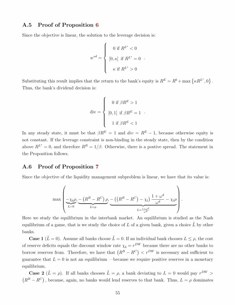
A.5 Proof of Proposition 6

Since the objective is linear, the solution to the leverage decision is:

w∗d =

0 if RL∗ < 0

[0, κ] if RL∗ = 0

κ if RL∗ > 0

.

Substituting this result implies that the return to the bank’s equity is RE = Rb + maxκRL∗ , 0

.

Thus, the bank’s dividend decision is:

div =

0 if βRE > 1

[0, 1] if βRE = 1

1 if βRE < 1

.

In any steady state, it must be that βRE = 1 and div = RE − 1, because otherwise equity is

not constant. If the leverage constraint is non-binding in the steady state, then by the condition

above RL∗ = 0, and therefore RB = 1/β. Otherwise, there is a postive spread. The statement in

the Proposition follows.

A.6 Proof of Proposition 7

Since the objective of the liquidity management subproblem is linear, we have that its value is:

max

−χbρ︸ ︷︷ ︸L=0

,−(RB −RC

)ρ︸ ︷︷ ︸

L=ρ

,−((RB −RC

)− χl

) 1 + ωd

ωd− χlρ︸ ︷︷ ︸

L= 1+ωd

ωd

.

Here we study the equilibrium in the interbank market. An equilibrium is studied as the Nash

equilibrium of a game, that is we study the choice of L of a given bank, given a choice L by other

banks.

Case 1 (L = 0). Assume all banks choose L = 0. If an individual bank chooses L ≤ ρ, the cost

of reserve deficits equals the discount window rate χb = rDW because there are no other banks to

borrow reserves from. Therefore, we have that(RB −RC

)< rDW is necessary and sufficient to

guarantee that L = 0 is not an equilibrium —because we require positive reserves in a monetary

equilibrium.

Case 2 (L = ρ). If all banks chooses L = ρ, a bank deviating to L = 0 would pay rDW >(RB −RC

), because, again, no banks would lend reserves to that bank. Thus, L = ρ dominates

55

L = 0 when other banks choose L = ρ and rDW >(RB −RC

). This shows that

(RB −RC

)< rDW

is neccesary and sufficient to guarantee that L = 0 not an equilibrium when L = ρ.

So far,(RB −RC

)< rDW is enough to argue that L ≥ ρ in a symmetric Nash equlibrium.

Assume now that also(RB −RC

)> rER holds.

Case 3 (L = 1+ωd

ωd). If all banks set L = 1+ωd

ωd> ρ, no bank will be short of reserves. Thus,

χl = rER since γ+ = 0. Thus, an individual banks is better off deviating by reducing L to ρ.

Case 4 (L = ρ). Instead, if all banks set L = ρ, then, χl = rER since again γ+ = 0. Thus,

L = ρ is an optimal choice because deviating to 1+ωd

ωdis not profitable.

Hence, rERt < RB − RC < rDWt will hold in any equilibrium with positive reserves and this

implies L∗ = ρ.

56

B Evolution of Bank Equity Distribution

Because the economy displays equity growth, equity is unbounded and thus, the support of this

measure is the positive real line. Let B be the Borel σ-algebra on the positive real line. Then,

define Qt(e,E) as the probability that an individual bank with current equity e transits to the set

E next period. Formally Qt : R+ × B → [0, 1], and

Q(e,E) =

∫ 1

−1

I et (ω) e ∈ EF (dω)

where I is the indicator function of the event in brackets. Then Q is a transition function and the

associated T ∗ operator for the evolution of bank equity is given by:

Γt+1 (E) =

∫ 1

0

Q(e,E)Γt+1 (e) de.

The distribution of equity is fanning out and the operator is unbounded. Gibrat’s law shows

that for t large enough Γt+1 is approximated by a log-normal distribution. Moreover, by introduc-

ing more structure into the problem, we could easily obtain a Power law distribution for Γt+1 (E).

We will use this properties in the calibrated version of the model.

57

C Algorithm

C.1 Steady State

1. Guess prices for loans q and for the probability of a match in the interbank market γ−, γ+.

2. Solve bank optimization problem 3. Compute value of the bank and dividend payments.

3. Compute associated average equity growth and average surplus in the interbank market.

4. If equity growth equals zero and the conjectured probability of a match in the interbank

market is consistent with the average surplus, stop. Otherwise, adjust and continue iterating.

Algorithm to solve transition dynamics in baseline model

C.2 Transitional Dynamics

1. Guess a sequence of loan prices qt and for the probability of a match in the interbank market

γ−t ,γ+t .

2. Solve by backward induction banks’s dynamic programming problem using 3 for banks’

portfolio and 4 for value function and dividend rates.

3. Compute growth rate of equity and average surplus in interbank markets.

4. Compute price implied by aggregate sequence of loans resulting from (2) and (3), and the

probability of a match according to average surpluses computed in (3).

5. If the conjectured price equal effective price from (4) and the average surplus computed

in (4) are consistent with the guessed sequences, stop. Otherwise, continue iterating until

convergence.

58

D Microfoundation for Loan Demand and Deposit Supply

There are multiple ways to introduce a demand for loans and a supply of deposits. Here, the

demand for loans emerges from firms who borrow working capital from banks and the supply of

deposits from the households’s savings decision. With working capital constraints, a low price

for loans, qt, translates immediately into labor market distortions and, therefore, has real output

effects. This formulation is borrowed from the classic setup of Christiano and Eichenbaum (1992).

To keep the model simple, we deliberately model the real sector so that the loans demand is static

—in the sense that it does not depend on future outcomes— and the supply of loans is perfectly

elastic.

D.1 Households

Households’s Problem. Households obtain utility by consuming and disutility from providing

labor. They work during the lending stage and consume during the balancing stage. This dis-

tinction is irrelevant for households but matters for the sequence of events that we describe later.

Households have quasi-linear utility in consumption and have a convex cost of providing labor

given byh1+νt

1+ν. The only savings instruments available to households are bank deposits and their

holding of shares of firms. Households solve the following recursive problem:

W (st, dt;Xt) = maxct≥0,ht,dt+1≥0

ct −h1+νt

1 + ν+ βDE [W (st+1, dt+1;Xt+1) |Xt]

subject to the budget constraint:

dt+1 + ct + pstst+1 = st(zt + pst) + wtht +RDt dt + Tt.

Here, βD is the households’s discount factor and ν the inverse of the Frisch elasticity. In the

budget constraint, dt are deposits in banks that earn a real rate of RD, ht are hours worked that

earn a wage of wt, and st are shares of productive firms. The price of shares is pst and these

pay zt dividends per share. Finally, ct is consumption and T are lump sum transfers from the

government.

The first-order conditions for the households’s problem yield the following labor supply:

w1νt = ht.

This supply schedule is static and only a function of real wages. Hence, the total wage income

for the household is w1+νν

t . In turn, substituting the optimality condition in this problem and

using the fact that in equilibrium st+1 = st, we can solve for the optimal policy decisions, c, d ,

59

independently from the labor choice. The solution is immediate and given by,

c, d =

ct = w

1+νν

t +RDdt + T ; dt+1 = 0 if RD < 1/βD,

ct ∈ [0, yt] , dt+1 = yt − ct if RD = 1/βD

ct = 0; d′ = w1+νν

t +RDdt + Tt if RD > 1/βD

These two results imply that households consume all cash on hand in the period they receive it

if the interest is very low and they do not save, or carry real balances. If RD = 1/βD, they are

indifferent between consuming or savings. Otherwise, they either do not consume or save all of

their resources. We will consider parameterizations where in equilibrium RD = 1/βD.

D.2 Firm’s Problem

Firms. Firms maximize E [∑∞

t=0mtzt] where zt are dividend payouts from the firms and µt is the

stochastic discount factor of the representative household. Given the linearity of the households’s

objective, the discount factor is equivalent to mt = (βD)t.

Timing. A continuum of firms of measure one is created at the lending stage of every period.

Firms choose a production scale together with a loan size during their arrival period. In periods

after this scale choice is decided, firms produce , pay back loans to banks; the residual is paid in

dividends.

Production Technology. A firm created in period t uses labor ht, to produce output accord-

ing to ft (ht) ≡ Ath1−αt . The scale of production is decided during the lending stage of the period

when the firm is created. Although the scale of production is determined immediately at the time

of creation, output takes time to be realized. In particular, the firm produces δs (1− δ) ft (ht) of

its output during the s-th balancing stage after its scale was decided.

Labor is also employed when the firm is created, and workers require to be paid at that

moment.42 Since firms do not possess the cash flow to pay their workers —no equity injections

are possible—firms need to borrow from banks to finance the payroll. Firms issue liabilities to the

banking sector —loans— by, lt, in exchange for deposits —bank liabilities—, qtlt, that firms can

use immediately to pay workers. The repayment of those loans occurs over time. In particular, firm

repay δs (1− δ) lt during the s-th lending stage after the loan was made. Notice that the repayment

rate δ coincides exactly with the δ rate of sales. This delivers a problem for firms similar to the

one in Christiano and Eichenbaum (1992) with the difference in the maturity. Taking as given

wages a labor tax τ l, and the loan prices qt, the problem of the firm created during the period t

42This constraint emerges if it is possible that the firm defaults on this promise and defaults on its payrollBigio (2011). The implicit assumption is that banks have a special advantage of monitoring loans compared tohouseholds.

60

is:

maxht,lt

∞∑s=1

(βD)s−1zt+s−1

subject to:

zt+s−1 = δs (1− δ)Atft (ht)− δs (1− δ) lt

and (1 + τ lt

)wtht = qtlt.

Substituting zt+s−1 into the objective function, and substituting the working capita loan, yields a

static maximization problem for firms:

maxht

Ath1−αt −

(1 + τ lt

)wtht/qt

Taking first-order conditions from this problem and the household’s first-order condition, wtht =

h1+νt , yields an allocation for labor

ht =

[qtAt (1− α)(

1 + τ lt) ] 1

α+ν

.

Now, using the working capital constraint,(1 + τ lt

)wtht = ltqt, and the expression above:

(1 + τ lt

) [qtAt (1− α)(1 + τ lt

) ] 1+να+ν

= ltqt.

Clearing qt from this expression yields:

lt = (At (1− α))1+να+ν((

1 + τ lt)qt) 1−αα+ν .

This is the expression in equation (7) and proves the following proposition:

Proposition 9 The demand for loans takes the form:

qt = ΘtIεt

where

Θt =(1 + τ lt

)[At (1− α)]−

1+ν1−α and ε =

(α + ν)

(1− α).

Standard calibrations assume α = 13

and some ν ∈[

13, 2]. This provides the bounds ε ∈

[1.0, 3.5].

61

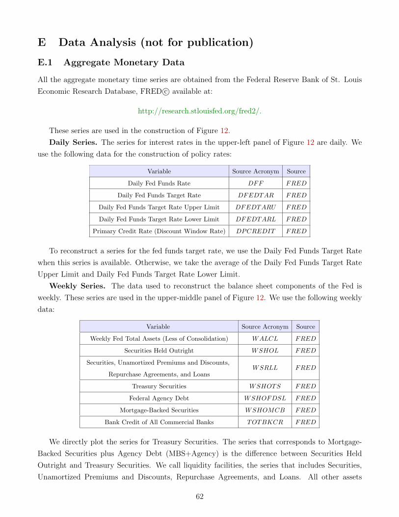
E Data Analysis (not for publication)

E.1 Aggregate Monetary Data

All the aggregate monetary time series are obtained from the Federal Reserve Bank of St. Louis

Economic Research Database, FRED c© available at:

http://research.stlouisfed.org/fred2/.

These series are used in the construction of Figure 12.

Daily Series. The series for interest rates in the upper-left panel of Figure 12 are daily. We

use the following data for the construction of policy rates:

Variable Source Acronym Source

Daily Fed Funds Rate DFF FRED

Daily Fed Funds Target Rate DFEDTAR FRED

Daily Fed Funds Target Rate Upper Limit DFEDTARU FRED

Daily Fed Funds Target Rate Lower Limit DFEDTARL FRED

Primary Credit Rate (Discount Window Rate) DPCREDIT FRED

To reconstruct a series for the fed funds target rate, we use the Daily Fed Funds Target Rate

when this series is available. Otherwise, we take the average of the Daily Fed Funds Target Rate

Upper Limit and Daily Fed Funds Target Rate Lower Limit.

Weekly Series. The data used to reconstruct the balance sheet components of the Fed is

weekly. These series are used in the upper-middle panel of Figure 12. We use the following weekly

data:

Variable Source Acronym Source

Weekly Fed Total Assets (Less of Consolidation) WALCL FRED

Securities Held Outright WSHOL FRED

Securities, Unamortized Premiums and Discounts,

Repurchase Agreements, and LoansWSRLL FRED

Treasury Securities WSHOTS FRED

Federal Agency Debt WSHOFDSL FRED

Mortgage-Backed Securities WSHOMCB FRED

Bank Credit of All Commercial Banks TOTBKCR FRED

We directly plot the series for Treasury Securities. The series that corresponds to Mortgage-

Backed Securities plus Agency Debt (MBS+Agency) is the difference between Securities Held

Outright and Treasury Securities. We call liquidity facilities, the series that includes Securities,

Unamortized Premiums and Discounts, Repurchase Agreements, and Loans. All other assets

62

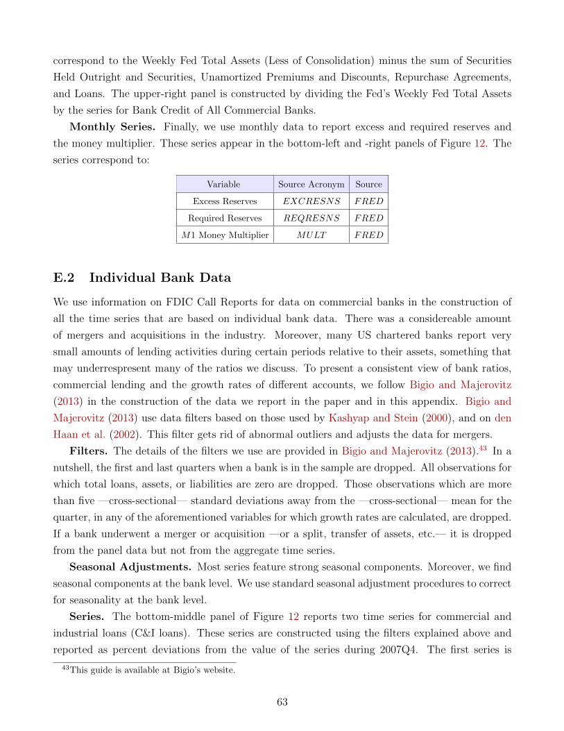
correspond to the Weekly Fed Total Assets (Less of Consolidation) minus the sum of Securities

Held Outright and Securities, Unamortized Premiums and Discounts, Repurchase Agreements,

and Loans. The upper-right panel is constructed by dividing the Fed’s Weekly Fed Total Assets

by the series for Bank Credit of All Commercial Banks.

Monthly Series. Finally, we use monthly data to report excess and required reserves and

the money multiplier. These series appear in the bottom-left and -right panels of Figure 12. The

series correspond to:

Variable Source Acronym Source

Excess Reserves EXCRESNS FRED

Required Reserves REQRESNS FRED

M1 Money Multiplier MULT FRED

E.2 Individual Bank Data

We use information on FDIC Call Reports for data on commercial banks in the construction of

all the time series that are based on individual bank data. There was a considereable amount

of mergers and acquisitions in the industry. Moreover, many US chartered banks report very

small amounts of lending activities during certain periods relative to their assets, something that

may underrespresent many of the ratios we discuss. To present a consistent view of bank ratios,

commercial lending and the growth rates of different accounts, we follow Bigio and Majerovitz

(2013) in the construction of the data we report in the paper and in this appendix. Bigio and

Majerovitz (2013) use data filters based on those used by Kashyap and Stein (2000), and on den

Haan et al. (2002). This filter gets rid of abnormal outliers and adjusts the data for mergers.

Filters. The details of the filters we use are provided in Bigio and Majerovitz (2013).43 In a

nutshell, the first and last quarters when a bank is in the sample are dropped. All observations for

which total loans, assets, or liabilities are zero are dropped. Those observations which are more

than five —cross-sectional— standard deviations away from the —cross-sectional— mean for the

quarter, in any of the aforementioned variables for which growth rates are calculated, are dropped.

If a bank underwent a merger or acquisition —or a split, transfer of assets, etc.— it is dropped

from the panel data but not from the aggregate time series.

Seasonal Adjustments. Most series feature strong seasonal components. Moreover, we find

seasonal components at the bank level. We use standard seasonal adjustment procedures to correct

for seasonality at the bank level.

Series. The bottom-middle panel of Figure 12 reports two time series for commercial and

industrial loans (C&I loans). These series are constructed using the filters explained above and

reported as percent deviations from the value of the series during 2007Q4. The first series is

43This guide is available at Bigio’s website.

63

the time series for commercial and industrial loans. The other series adjusts the original series

for increases in lending that have to do with prior commitments. The series adjusted for prior

commitments and is constructed the following way. First, we construct an upper bound for the use

of loan commitments, subtracting the value of the stock of loan commitments at a given quarter

from the stock during 2007Q4. Then, the adjusted series for C&I loans is the original series minus

the series for the use of loan commitments.

The following section of this appendix describes some statistics for several bank balance-sheet

accounts. That analysis guides our judgements of using total deposits to calibrate the withdrawal

distribution, Ft, in our model. We narrow the analysis to the statistics of total deposits (TD),

demand deposits (DD), total liabilities (TL), tangible equity (TE), equity (E), and loans net of

unearned income (LNUI).

Bank Ratios. The bank ratios reported in Figure 13 are the following: Tangible leverage

is the value of total liabilities minus intangibles over the value of equity minus intangibles. The

liquidity ratio is constructed as the sum of reserves (cash) plus treasury securities over total assets.

The dividend rate is the value of dividends relative to equity. The series for the return on equity

is income over the value of equity. We report the cross-sectional average for every bank and every

quarter in the cross section. We report two averages, simple averages and averages weighted by

asset size.

Summary of Individual Variables. The summary of the series we use is found here:

Variable Source Acronym Source

total deposits (TD) rcfd2200 Call Reports

demand deposits (DD) rcfd2948 Call Reports

total liabilities (TL) rcfd2948 Call Reports

intangible rcfd2143 Call Reports

cash rcfd0010 Call Reports

treasury holdings rcfd0400+rcfd8634 Call Reports

tangible equity (TE) Equity Intangible Call Reports

equity (E) TotalAssets-TotalLiability Call Reports

total loans

net of unearned income (LNUI)rcfd2122 Call Reports

commercial and industrial loans rcfd1766 Call Reports

commercial and industrial loans (commitments) rcfd3816+rcfd6550 Call Reports

total assets rcfd2170 Call Reports

income riad4000 Call Reports

dividends riad4460+riad4470 Call Reports

64

E.3 Data Analysis

1990-2010 Sample Averages. The summary statistics for the quarterly growth rate of the

aggregate time series is presented in Table 3.

Table 3: Summary statistics for quarter-bank observations

Variable Mean Std. Dev. N

TD 1.018 0.064 536074

DD 1.027 0.810 536074

TL 1.018 0.063 536074

TE 1.018 0.058 536074

E 1.019 0.067 536074

LNUI 1.022 0.061 536074

The data exhibits very similar patterns when we compare the average growth and standard

deviation of the growth rate of total deposits and total liabilities. Demand deposits, on the

contrary, are almost ten times as volatile as total deposits. This is one reason to use total deposits

as our data counterpart for calibrate Ft. Although less volatile than demand deposits, total deposits

still feature substantial volatility. The standard deviation of this series is 6.4 percent per quarter,

and it is close to the volatility of total liabilities, 6.3 percent. Total deposits are also more

correlated with equity growth —both for tangible and total equity. The correlation matrix of the

variables in the analysis is reported in Table 4.

Quarterly Cross-Sectional Deviations. Part of the variation in the bank-quarter statis-

tics presented above follow from the influence of aggregate trends and seasonal components. To

decompose the variation of these liabilities into their common trend, we present the summary

statistics in terms of deviations of these variables from their quarterly cross-sectional averages.

Table 5 presents the summary for cross-sectional deviations.

A comparison between tables 3 and 5 reveals that the series for deviations from the cross-

sectional mean preserve much of the variation of the aggregated time series. This is evidence

65

Table 4: Cross-sectional correlation for quarter-bank observations

Variables TD DD TL TE E LNUI

TD 1.000

DD 0.059 1.000

TL 0.286 0.050 1.000

TE 0.117 0.005 0.102 1.000

E 0.145 0.006 0.098 0.855 1.000

LNUI 0.527 0.024 0.198 0.153 0.155 1.000

Table 5: Summary statistics for cross-sectional deviations from mean growth

Variable Mean Std. Dev. N

devTD 0 0.043 536074

devDD 0 0.123 536074

devTL 0 0.042 536074

devTE 0 0.039 536074

devE 0 0.041 536074

devLNUI 0 0.045 536074

66

of a fairamount of idiosyncratic volatility in total deposit growth accross banks. Table 6 shows

the correlation in cross-sectional deviations from quarterly means accross these varaibles. These

correlations are almost identical to the correlations of historical growth rates. This implies that

the idiosyncratic component is very important to explain the cross-correlations, more so than

common aggregate treds.

Table 6: Correlation for Cross-Sectional Deviations from Means

Variables dev TD dev DD G dev TL dev TE dev RTE dev E dev RE

dev T D 1.000

dev DD 0.389 1.000

dev TL 0.844 0.345 1.000

dev TE 0.082 0.027 0.135 1.000

dev RTE 0.050 0.016 0.097 0.854 1.000

dev E 0.152 0.052 0.238 0.727 0.635 1.000

dev RE 0.118 0.040 0.187 0.635 0.769 0.881 1.000

The correlation between the cross-sectional deviations of tangible equity growth and the coun-

terpart for total deposits 8.2 percent. In the model, this correlation is very high —though not 1

do to the kink in χ (·)— because deposit volatility is the only source of risk for banks. In practice,

banks face other sources of risks which include loan risk, duration risk, and trading risk. This

figure, however, suggests that deposit withdrawal risks are non-negligible risks for banks. Figure

1, found in the body of the paper, reports the empirical histograms for every bank-quarter growth

observation and decomposes the data into two samples, pre-crisis (1990Q1-2007Q4) and crisis

(2008Q1-2010Q4). We use the empirical histogram of the quarterly deviations of total deposits to

calibrate Ft, the process for withdrawal shocks.

Tests for Growth Independence. We have a assumed that the withdrawal process is i.i.d.

over time and accross banks. This assumption is critical to solve the model without keeping track

of distributions. This assumption implies that if we substract the common growth rates of all

the balance sheet variables in our model, the residual should be serially uncorrelated. We test

the independence of the deviations-from-means quarterly growth rates using an OLS estimation

procedure. We run the deviations in quarterly growth rates from the cross-sectional averages

against their lags. The evidence from OLS autoregressions does not support the assumption

that of time-independent growth because autocorrelations are significant. Table 7 reports the

autocorrelation coefficients of all the variables in deviations. Though none are statistically equal

67

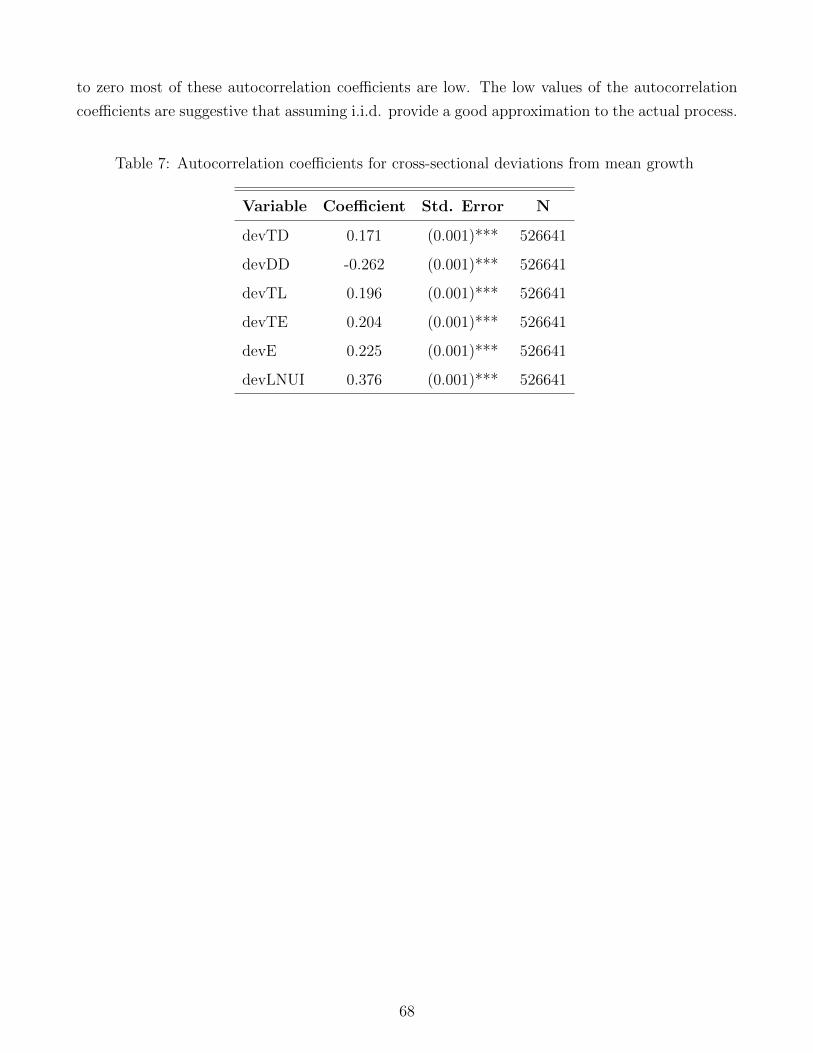
to zero most of these autocorrelation coefficients are low. The low values of the autocorrelation

coefficients are suggestive that assuming i.i.d. provide a good approximation to the actual process.

Table 7: Autocorrelation coefficients for cross-sectional deviations from mean growth

Variable Coefficient Std. Error N

devTD 0.171 (0.001)*** 526641

devDD -0.262 (0.001)*** 526641

devTL 0.196 (0.001)*** 526641

devTE 0.204 (0.001)*** 526641

devE 0.225 (0.001)*** 526641

devLNUI 0.376 (0.001)*** 526641

68