Embed Size (px)
Citation preview
Communication-Rounds Tradeoffs for Common Randomness and
Secret Key Generation
Mitali Bafna∗ Badih Ghazi† Noah Golowich‡ Madhu Sudan§
August 27, 2018
Abstract
We study the role of interaction in the Common Randomness Generation (CRG) and SecretKey Generation (SKG) problems. In the CRG problem, two players, Alice and Bob, respec-tively get samples X1, X2, . . . and Y1, Y2, . . . with the pairs (X1, Y1), (X2, Y2), . . . being drawnindependently from some known probability distribution µ. They wish to communicate so as toagree on L bits of randomness. The SKG problem is the restriction of the CRG problem to thecase where the key is required to be close to random even to an eavesdropper who can listen totheir communication (but does not have access to the inputs of Alice and Bob). In this work,we study the relationship between the amount of communication and the number of roundsof interaction in both the CRG and the SKG problems. Specifically, we construct a family ofdistributions µ = µr,n,L, parametrized by integers r, n and L, such that for every r there existsa constant b = b(r) for which CRG (respectively SKG) is feasible when (Xi, Yi) ∼ µr,n,L withr+ 1 rounds of communication, each consisting of O(log n) bits, but when restricted to r/2− 3rounds of interaction, the total communication must exceed Ω(n/ logb(n)) bits. Prior to ourwork no separations were known for r ≥ 2.
∗Harvard John A. Paulson School of Engineering and Applied Sciences, 33 Oxford Street, Cambridge, MA 02138,USA. [email protected]. Work supported in part by a Simons Investigator Award and NSF Award CCF1715187.†Google Research, 1600 Amphitheatre Parkway Mountain View, CA 94043, USA. [email protected] This
work was partly done while the author was a student at MIT. Supported in parts by NSF CCF-1650733 and CCF-1420692.‡Harvard University. [email protected]§Harvard John A. Paulson School of Engineering and Applied Sciences, 33 Oxford Street, Cambridge, MA 02138,
USA. [email protected]. Work supported in part by a Simons Investigator Award and NSF Award CCF1715187.
Contents
1 Introduction 11.1 Problem Definition . . . . . . . . . . . . . . . . . . . . . . . . . . . . . . . . . . . . . 11.2 History . . . . . . . . . . . . . . . . . . . . . . . . . . . . . . . . . . . . . . . . . . . 21.3 Our Results . . . . . . . . . . . . . . . . . . . . . . . . . . . . . . . . . . . . . . . . . 31.4 Brief Overview of Construction and Proofs . . . . . . . . . . . . . . . . . . . . . . . 4
2 Construction 6
3 Related Indistinguishability Problems 73.1 The Main Distributions and Indistinguishability Claims . . . . . . . . . . . . . . . . 83.2 Reduction to Common Randomness Generation . . . . . . . . . . . . . . . . . . . . . 83.3 Reduction to the Case t = 1 . . . . . . . . . . . . . . . . . . . . . . . . . . . . . . . . 10
4 The Pointer Verification Problem 10
5 Proof of Theorem 4.2 135.1 Preliminaries: Information-Theoretic Inequalities . . . . . . . . . . . . . . . . . . . . 135.2 A Reformulation of Theorem 4.2 . . . . . . . . . . . . . . . . . . . . . . . . . . . . . 145.3 Proof of the Main Lemma (Lemma 5.5): Setting up the Induction . . . . . . . . . . 155.4 The Base Case: Proof of Lemma 5.11 . . . . . . . . . . . . . . . . . . . . . . . . . . 195.5 The Inductive Step: Proof of Lemma 5.9 . . . . . . . . . . . . . . . . . . . . . . . . . 27
1 Introduction
1.1 Problem Definition
In this work, we study the Common Randomness Generation (CRG) and Secret Key Generation(SKG) problems — two central questions in information theory, distributed computing and cryp-tography — and study the need for interaction in solving these problems.
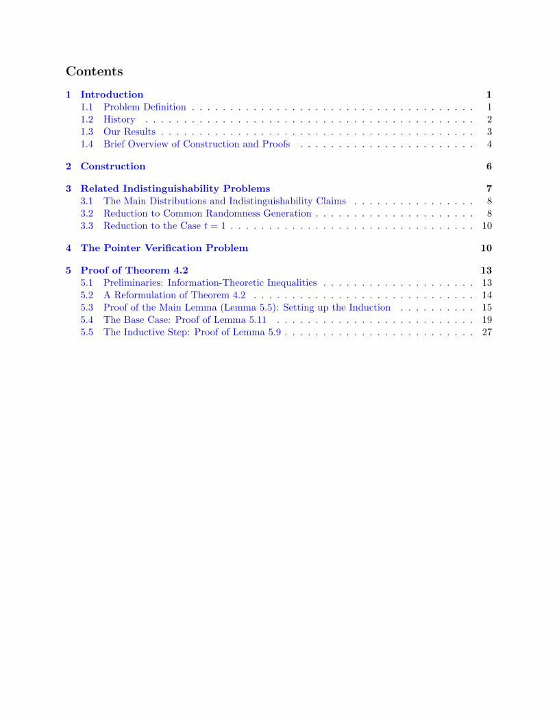
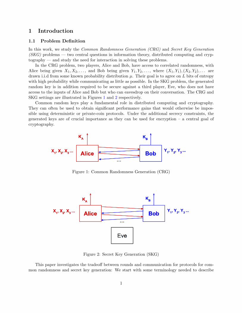
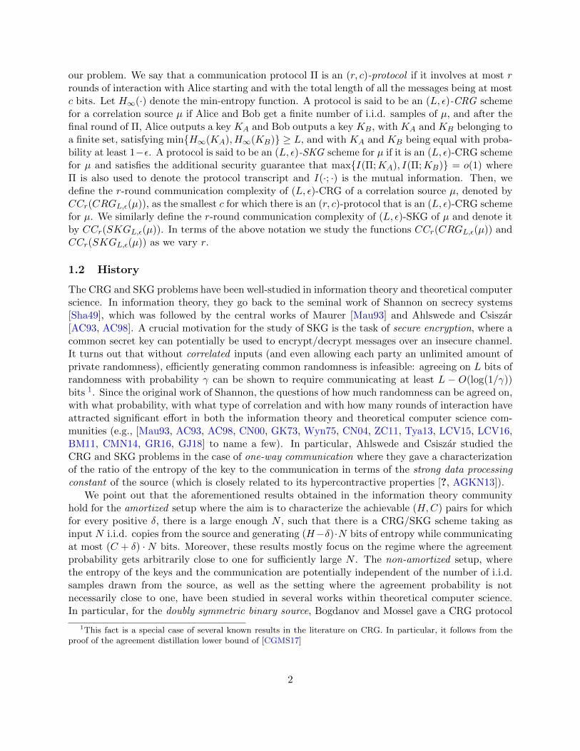
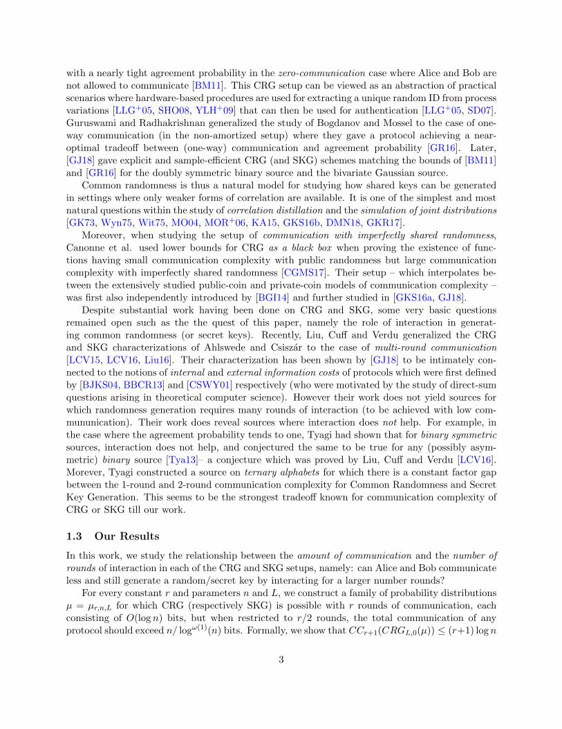
In the CRG problem, two players, Alice and Bob, have access to correlated randomness, withAlice being given X1, X2, . . . , and Bob being given Y1, Y2, . . . , where (X1, Y1), (X2, Y2), . . . aredrawn i.i.d from some known probability distribution µ. Their goal is to agree on L bits of entropywith high probability while communicating as little as possible. In the SKG problem, the generatedrandom key is in addition required to be secure against a third player, Eve, who does not haveaccess to the inputs of Alice and Bob but who can eavesdrop on their conversation. The CRG andSKG settings are illustrated in Figures 1 and 2 respectively.
Common random keys play a fundamental role in distributed computing and cryptography.They can often be used to obtain significant performance gains that would otherwise be impos-sible using deterministic or private-coin protocols. Under the additional secrecy constraints, thegenerated keys are of crucial importance as they can be used for encryption – a central goal ofcryptography.
Figure 1: Common Randomness Generation (CRG)
Figure 2: Secret Key Generation (SKG)
This paper investigates the tradeoff between rounds and communication for protocols for com-mon randomness and secret key generation: We start with some terminology needed to describe
1
our problem. We say that a communication protocol Π is an (r, c)-protocol if it involves at most rrounds of interaction with Alice starting and with the total length of all the messages being at mostc bits. Let H∞(·) denote the min-entropy function. A protocol is said to be an (L, ε)-CRG schemefor a correlation source µ if Alice and Bob get a finite number of i.i.d. samples of µ, and after thefinal round of Π, Alice outputs a key KA and Bob outputs a key KB, with KA and KB belonging toa finite set, satisfying minH∞(KA), H∞(KB) ≥ L, and with KA and KB being equal with proba-bility at least 1−ε. A protocol is said to be an (L, ε)-SKG scheme for µ if it is an (L, ε)-CRG schemefor µ and satisfies the additional security guarantee that maxI(Π;KA), I(Π;KB) = o(1) whereΠ is also used to denote the protocol transcript and I(·; ·) is the mutual information. Then, wedefine the r-round communication complexity of (L, ε)-CRG of a correlation source µ, denoted byCCr(CRGL,ε(µ)), as the smallest c for which there is an (r, c)-protocol that is an (L, ε)-CRG schemefor µ. We similarly define the r-round communication complexity of (L, ε)-SKG of µ and denote itby CCr(SKGL,ε(µ)). In terms of the above notation we study the functions CCr(CRGL,ε(µ)) andCCr(SKGL,ε(µ)) as we vary r.
1.2 History
The CRG and SKG problems have been well-studied in information theory and theoretical computerscience. In information theory, they go back to the seminal work of Shannon on secrecy systems[Sha49], which was followed by the central works of Maurer [Mau93] and Ahlswede and Csiszar[AC93, AC98]. A crucial motivation for the study of SKG is the task of secure encryption, where acommon secret key can potentially be used to encrypt/decrypt messages over an insecure channel.It turns out that without correlated inputs (and even allowing each party an unlimited amount ofprivate randomness), efficiently generating common randomness is infeasible: agreeing on L bits ofrandomness with probability γ can be shown to require communicating at least L − O(log(1/γ))bits 1. Since the original work of Shannon, the questions of how much randomness can be agreed on,with what probability, with what type of correlation and with how many rounds of interaction haveattracted significant effort in both the information theory and theoretical computer science com-munities (e.g., [Mau93, AC93, AC98, CN00, GK73, Wyn75, CN04, ZC11, Tya13, LCV15, LCV16,BM11, CMN14, GR16, GJ18] to name a few). In particular, Ahlswede and Csiszar studied theCRG and SKG problems in the case of one-way communication where they gave a characterizationof the ratio of the entropy of the key to the communication in terms of the strong data processingconstant of the source (which is closely related to its hypercontractive properties [?, AGKN13]).
We point out that the aforementioned results obtained in the information theory communityhold for the amortized setup where the aim is to characterize the achievable (H,C) pairs for whichfor every positive δ, there is a large enough N , such that there is a CRG/SKG scheme taking asinput N i.i.d. copies from the source and generating (H−δ)·N bits of entropy while communicatingat most (C + δ) ·N bits. Moreover, these results mostly focus on the regime where the agreementprobability gets arbitrarily close to one for sufficiently large N . The non-amortized setup, wherethe entropy of the keys and the communication are potentially independent of the number of i.i.d.samples drawn from the source, as well as the setting where the agreement probability is notnecessarily close to one, have been studied in several works within theoretical computer science.In particular, for the doubly symmetric binary source, Bogdanov and Mossel gave a CRG protocol
1This fact is a special case of several known results in the literature on CRG. In particular, it follows from theproof of the agreement distillation lower bound of [CGMS17]
2
with a nearly tight agreement probability in the zero-communication case where Alice and Bob arenot allowed to communicate [BM11]. This CRG setup can be viewed as an abstraction of practicalscenarios where hardware-based procedures are used for extracting a unique random ID from processvariations [LLG+05, SHO08, YLH+09] that can then be used for authentication [LLG+05, SD07].Guruswami and Radhakrishnan generalized the study of Bogdanov and Mossel to the case of one-way communication (in the non-amortized setup) where they gave a protocol achieving a near-optimal tradeoff between (one-way) communication and agreement probability [GR16]. Later,[GJ18] gave explicit and sample-efficient CRG (and SKG) schemes matching the bounds of [BM11]and [GR16] for the doubly symmetric binary source and the bivariate Gaussian source.
Common randomness is thus a natural model for studying how shared keys can be generatedin settings where only weaker forms of correlation are available. It is one of the simplest and mostnatural questions within the study of correlation distillation and the simulation of joint distributions[GK73, Wyn75, Wit75, MO04, MOR+06, KA15, GKS16b, DMN18, GKR17].
Moreover, when studying the setup of communication with imperfectly shared randomness,Canonne et al. used lower bounds for CRG as a black box when proving the existence of func-tions having small communication complexity with public randomness but large communicationcomplexity with imperfectly shared randomness [CGMS17]. Their setup – which interpolates be-tween the extensively studied public-coin and private-coin models of communication complexity –was first also independently introduced by [BGI14] and further studied in [GKS16a, GJ18].
Despite substantial work having been done on CRG and SKG, some very basic questionsremained open such as the the quest of this paper, namely the role of interaction in generat-ing common randomness (or secret keys). Recently, Liu, Cuff and Verdu generalized the CRGand SKG characterizations of Ahlswede and Csiszar to the case of multi-round communication[LCV15, LCV16, Liu16]. Their characterization has been shown by [GJ18] to be intimately con-nected to the notions of internal and external information costs of protocols which were first definedby [BJKS04, BBCR13] and [CSWY01] respectively (who were motivated by the study of direct-sumquestions arising in theoretical computer science). However their work does not yield sources forwhich randomness generation requires many rounds of interaction (to be achieved with low com-mununication). Their work does reveal sources where interaction does not help. For example, inthe case where the agreement probability tends to one, Tyagi had shown that for binary symmetricsources, interaction does not help, and conjectured the same to be true for any (possibly asym-metric) binary source [Tya13]– a conjecture which was proved by Liu, Cuff and Verdu [LCV16].Morever, Tyagi constructed a source on ternary alphabets for which there is a constant factor gapbetween the 1-round and 2-round communication complexity for Common Randomness and SecretKey Generation. This seems to be the strongest tradeoff known for communication complexity ofCRG or SKG till our work.
1.3 Our Results
In this work, we study the relationship between the amount of communication and the number ofrounds of interaction in each of the CRG and SKG setups, namely: can Alice and Bob communicateless and still generate a random/secret key by interacting for a larger number rounds?
For every constant r and parameters n and L, we construct a family of probability distributionsµ = µr,n,L for which CRG (respectively SKG) is possible with r rounds of communication, eachconsisting of O(log n) bits, but when restricted to r/2 rounds, the total communication of anyprotocol should exceed n/ logω(1)(n) bits. Formally, we show that CCr+1(CRGL,0(µ)) ≤ (r+1) log n
3
while for every constant ε < 1 we have that CCr/2−3(CRG`,ε) ≥ minΩ(`), n/poly log n (andsimilarly for SKG).
Theorem 1.1 (Communication-Rounds Tradeoff for Common Randomness Generation). For allε < 1, r ∈ Z+, there exist η > 0, n0, β < ∞, such that for all n ≥ n0, L there exists a source µr,n,Lfor which the following hold:
1. There exists an ((r + 1), (r + 1)dlog ne)-protocol for (L, 0)-CRG from µr,n,L.
2. For every ` ∈ Z+ there is no (r/2 − 2,minη` − β, n/ logβ n)-protocol for (`, ε)-CRG fromµr,n,L.
We also get an analogous theorem for SKG, with the same source!
Theorem 1.2 (Communication-Rounds Tradeoff for Secret Key Generation). For all ε < 1, r ∈ Z+,there exist η > 0, n0, β < ∞, such that for all n ≥ n0, L there exists a source µr,n,L for which thefollowing hold:
1. There exists an ((r + 1), (r + 1)dlog ne)-protocol for (L, 0)-SKG from µr,n,L.
2. For every ` ∈ Z+ there is no (r/2 − 2,minη` − β, n/ logβ n)-protocol for (`, ε)-SKG fromµr,n,L.
In particular, our theorems yield a gap in the amount of communication that is almost expo-nentially large if the number of rounds of communication is squeezed by a constant factor. Notethat every communication protocol can be converted to a two-round communication protocol withan exponential blowup in communication - so in this sense our bound is close to optimal. Prior toour work, no separations were known for any number of rounds larger than two!
1.4 Brief Overview of Construction and Proofs
Our starting point for constructing the source µ is the well-known “pointer-chasing” problem[NW93] used to study tradeoffs between rounds of interaction and communication complexity.In (our variant of) this problem Alice and Bob get a series of permutations π1, π2, . . . , πr : [n]→ [n]along with an initial pointer i0 and their goal is to “chase” the pointers, i.e., compute ir whereij = πj(ij−1) for every j ∈ 1, . . . , r. Alice’s input consists of the odd permutations π1, π3, . . . ,and Bob gets the initial pointer i0 and the even permutations π2, π4, . . .. The natural protocol todetermine ir takes r+ 1 rounds of communication with the jth round involving the message ij (forj = 0, . . . , r). Nisan and Wigderson show that any protocol with r rounds of interaction requiresΩ(n) bits of communication [NW93].
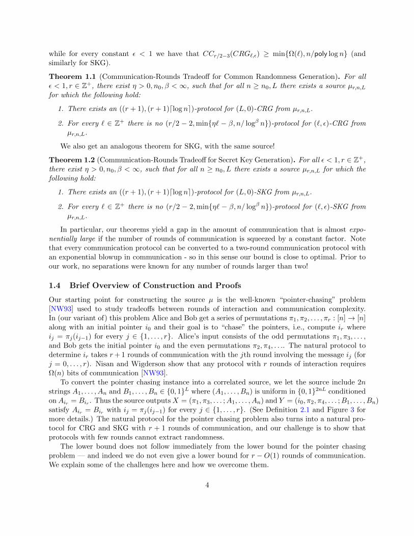
To convert the pointer chasing instance into a correlated source, we let the source include 2nstrings A1, . . . , An and B1, . . . , Bn ∈ 0, 1L where (A1, . . . , Bn) is uniform in 0, 12nL conditionedonAir = Bir . Thus the source outputsX = (π1, π3, . . . ;A1, . . . , An) and Y = (i0, π2, π4, . . . ;B1, . . . , Bn)satisfy Air = Bir with ij = πj(ij−1) for every j ∈ 1, . . . , r. (See Definition 2.1 and Figure 3 formore details.) The natural protocol for the pointer chasing problem also turns into a natural pro-tocol for CRG and SKG with r + 1 rounds of communication, and our challenge is to show thatprotocols with few rounds cannot extract randomness.
The lower bound does not follow immediately from the lower bound for the pointer chasingproblem — and indeed we do not even give a lower bound for r −O(1) rounds of communication.We explain some of the challenges here and how we overcome them.
4
Our first challenge is that there is a low-complexity “non-deterministic protocol” for commonrandomness generation in our setting. The players somehow guess ir and then verify Air = Bir(by exchanging the first log 1/ε bits of these strings) and if they do, then they output Air andBir respectively. While the existence of a non-deterministic protocol does not imply the existenceof a deterministic one, it certainly poses hurdles to the lower bound proofs. Typical separationsbetween non-deterministic communication complexity and deterministic ones involve lower boundssuch as those for “set-disjointness” [KS92, Raz92, BJKS04] which involve different reasoning thanthe “round-elimination” arguments in [NW93]. Our lower bound would somehow need to combinethe two approaches.
We manage to do so “modularly” at the expense of a factor of 2 in the number of roundsof communication by introducing an intermediate “pointer verification (PV)” problem. In thisproblem Alice and Bob get permutations π1, . . . , πr (with Alice getting the odd ones and Bob theeven ones) and additionally Bob gets pointers i and j. Their goal is to decide if the final pointer irequals j given that the initial pointer i0 is equal to i. The usefulness of this problem comes fromthe fact that we can reduce the common randomness generation problem to the complexity of thepointer verification problem on a specific (and natural) distribution: Specifically if PV is hard onthis distribution with r′ rounds of communication, then we can show (using the hardness of setdisjointness as a black box) that the common randomness generation problem is hard with r′ − 1rounds of communication.
We thus turn to showing lower bounds for PV. We first note that we cannot expect a lowerbound for r rounds of communication: PV can obviously be solved in r/2 rounds of communicationwith Alice and Bob chasing both the initial and final pointers till they meet in the middle. We alsonote that one can use the lower bound from [NW93] as a black box to get a lower bound of r/2− 1rounds of communication for PV but it is no longer on the “natural” distribution we care aboutand thus this is not useful for our setting.
The bulk of this paper is thus devoted to proving an r/2−O(1) round lower bound for the PVproblem on our distribution. We get this lower bound by roughly following the “round elimination”strategy of [NW93]. A significant challenge in extending these lower bounds to our case is that wehave to deal with distributions where Alice and Bob’s inputs are dependent. This should not besurprising since the CRG problem provides Alice and Bob with correlated inputs, and so there isresulting dependency between Alice and Bob even before any messages are sent. The dependencygets more complex as Alice and Bob exchange messages, and we need to ensure that the resultingmutual information is not correlated with the desired output, i.e., the PV value of the game. We doso by a delicate collection of conditions (see Definition 5.6) that allow the inputs to be correlatedwhile guaranteeing sufficient independence to carry out a round elimination proof. See Section 5for details.
Organization of Rest of the Paper. In Section 2, we present our construction of the distri-bution µ alluded to in Theorem 1.1 and Theorem 1.2. In Section 3 we reduce the task of provingcommunication lower bounds for CRG with few rounds to the task of proving lower bounds fordistinguishing some distributions. We then introduce our final problem, the Pointer Verificationproblem, and the distribution on which we need to analyze it in Section 4. This section includesthe statement of our main technical theorem about the pointer verification problem (Theorem 4.2)and the proofs of Theorem 1.1 and Theorem 1.2 assuming this theorem. Finally in Section 5, weprove Theorem 4.2.
5
2 Construction
We start with some basic notation used in the rest of the paper. For any positive integer n, wedenote by [n] the set 1, . . . , n. We use log to denote the logarithm to the base 2. For a distributionD on a universe Ω we use the notation X ∼ D to denote a random variable X sampled according toD. For any positive integer t, we denote by Dt the distribution obtained by sampling t independentidentically distributed samples from D. We use the notation X |= Y to denote that X is independentof Y and X |= Y |Z to denote that X and Y are independent conditioned on Z. We denote byEX∼D[X] the expectation of X and for an event E ⊆ Ω, we denote by PrX [E] the probabilityof the event E. For i ∈ Ω, Di (and sometimes D(i)) denotes the probability of the element i,i.e., Di = D(i) = PrX∼D[X = i]. For distributions P and Q on Ω, the total variation distance
∆(P,Q)def= 1
2
∑i∈Ω |Pi −Qi|. The entropy of X ∼ P is the quantity H(X) = EX∼P [− logPX ]. The
min-entropy of X ∼ P is the quantity H∞(X) = minx∈Ω− logPx. For a pair of random variables(X,Y ) ∼ P , PX denotes the marginal distribution on X and PX|y denotes the distribution of X
conditioned on Y = y. The conditional entropy H(X|Y )def= Ey∼PY [H(Xy)], where Xy ∼ PX|Y=y.
The mutual information between X and Y , denoted I(X;Y ), is the quantity H(X) − H(X|Y ).The conditional mutual information between X and Y conditioned on Z, denoted I(X;Y |Z), isthe quantity Ez∼PZ [H(Xz) − H(Xz|Yz)] where (Xz, Yz) ∼ PX,Y |Z=z. We use standard propertiesof entropy and information such as the Chain rules and the fact “conditioning does not increaseentropy”. For further background material on information theory and communication complexity,we refer the reader to the books [CT12] and [KN97] respectively.
We start by describing the family of distributions µr,n,L that we use to prove Theorem 1.1 andTheorem 1.2. For a positive integer n, we let Sn denote the family of all permutations of [n].
Definition 2.1 (The Pointer Chasing Source µr,n,L). For positive integers r, n and L, the support of
µ = µr,n,L is (Sdr/2en ×0, 1nL)×([n]×Sbr/2cn ×0, 1nL). Denoting X = (π1, π3, . . . , π2dr/2e−1, A1, . . . , An)
and Y = (i, π2, π4, . . . , π2br/2c, B1, . . . , Bn), a sample (X,Y ) ∼ µ is drawn as follows:
• i ∈ [n] and π1, . . . , πr ∈ Sn are sampled uniformly and independently.
• Let j = πr(πr−1(· · ·π1(i) · · · )).
• Aj = Bj ∈ 0, 1L is sampled uniformly and independently of i and π’s.
• For every k 6= j, Ak ∈ 0, 1L and Bk ∈ 0, 1L are sampled uniformly and independently.
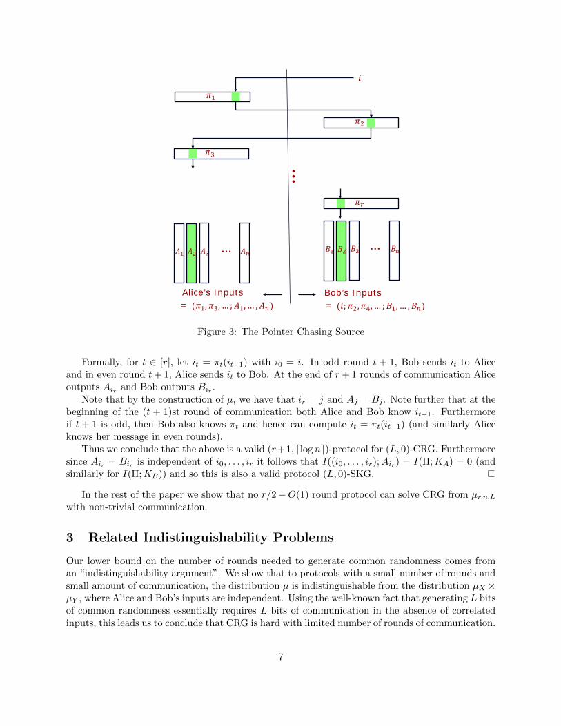
See Figure 3 for an illustration of the inputs to the Pointer Chasing Source.
Informally, a sample from µ contains a common hidden block of randomness Aj = Bj ∈ 0, 1Lthat Alice and Bob can find by following a sequence of pointers, where Alice holds the odd pointersin the sequence and Bob holds the even pointers. The next lemma gives (the obvious) upper boundon the r-round communication needed to generate common randomness from µ.
Lemma 2.2 (Upper bound on r-round communication of SKG). For every r, n and L, there existsan (r + 1, dlog ne)-protocol for (L, 0)-SKG (and hence also for (L, 0)-CRG) from µr,n,L with Bobspeaking in the first round.
Proof. The protocol Π is the obvious one in which Bob and Alice alternate by sending a pointer toeach other starting with i and culminating in j, and the randomness they “agree on” is Aj = Bj .
6
𝜋𝜋1
𝜋𝜋2
𝜋𝜋3
𝜋𝜋𝑟𝑟
𝑖𝑖
⋮
𝐴𝐴1 𝐴𝐴2 𝐴𝐴3 𝐴𝐴𝑛𝑛 𝐵𝐵1 𝐵𝐵2 𝐵𝐵3 𝐵𝐵𝑛𝑛… …
Alice’s Inputs= (𝜋𝜋1,𝜋𝜋3, … ;𝐴𝐴1, … ,𝐴𝐴𝑛𝑛)
Bob’s Inputs= (𝑖𝑖;𝜋𝜋2,𝜋𝜋4, … ;𝐵𝐵1, … ,𝐵𝐵𝑛𝑛)
Figure 3: The Pointer Chasing Source
Formally, for t ∈ [r], let it = πt(it−1) with i0 = i. In odd round t + 1, Bob sends it to Aliceand in even round t+ 1, Alice sends it to Bob. At the end of r+ 1 rounds of communication Aliceoutputs Air and Bob outputs Bir .
Note that by the construction of µ, we have that ir = j and Aj = Bj . Note further that at thebeginning of the (t + 1)st round of communication both Alice and Bob know it−1. Furthermoreif t + 1 is odd, then Bob also knows πt and hence can compute it = πt(it−1) (and similarly Aliceknows her message in even rounds).
Thus we conclude that the above is a valid (r+1, dlog ne)-protocol for (L, 0)-CRG. Furthermoresince Air = Bir is independent of i0, . . . , ir it follows that I((i0, . . . , ir);Air) = I(Π;KA) = 0 (andsimilarly for I(Π;KB)) and so this is also a valid protocol (L, 0)-SKG.
In the rest of the paper we show that no r/2−O(1) round protocol can solve CRG from µr,n,Lwith non-trivial communication.
3 Related Indistinguishability Problems
Our lower bound on the number of rounds needed to generate common randomness comes froman “indistinguishability argument”. We show that to protocols with a small number of rounds andsmall amount of communication, the distribution µ is indistinguishable from the distribution µX ×µY , where Alice and Bob’s inputs are independent. Using the well-known fact that generating L bitsof common randomness essentially requires L bits of communication in the absence of correlatedinputs, this leads us to conclude that CRG is hard with limited number of rounds of communication.
7
In this section we simply set up the stage by defining the notion of indistinguishability andconnecting it to the task of common randomness generation, leaving the task of proving the indis-tinguishability to later sections.
3.1 The Main Distributions and Indistinguishability Claims
We start by defining the indistinguishability of inputs to protocols.
Definition 3.1. We say that two distributions D1 and D2 on (X,Y ) are ε-indistinguishable toa protocol Π if the distributions of transcripts (the sequence of messages exchanged by Alice andBob) generated when (X,Y ) ∼ D1 has total variation distance at most ε from the distribution oftranscripts when (X,Y ) ∼ D2.
We say that distributions D1 and D2 are (ε, c, r)-indistinguishable if they are ε-indistinguishableto every (r, c)-protocol Π using public randomness. Conversely, we say that the distributions D1
and D2 are (ε, c, r)-distinguishable if they are not (ε, c, r)-indistinguishable.
Fix r, n, L and let µ = µr,n,L. Now let µX denote the marginal distribution of X under µ, i.e.,X = (π1, π3, . . . , π2dr/2e−1, A1, . . . , An) have all coordinates chosen independently and uniformlyfrom their domains. Similarly let µY denote the marginal on Y , and let µX × µY denote thedistribution where X ∼ µX and Y ∼ µY are chosen independently.
Our main technical result (Theorem 4.2 and in particular its implication Lemma 4.5) showsthat µ and µX ×µY are (ε, r/2−O(1), n/poly log n)-indistinguishable, even to protocols with com-mon randomness. In the rest of this section, we explain why this rules out common randomnessgeneration.
3.2 Reduction to Common Randomness Generation
Proposition 3.2. There exists a constant η > 0 such that for every r, r′, n, L, `, t and ε < 1, thereis no (r′, η` − log(1/1 − ε))-protocol for (`, ε)-CRG from µtX × µtY , where µ = µr,n,L with µX andµY being its marginals.
Proof. This is essentially folklore. For instance it follows immediately from [CGMS17, Theorem2.6] using ρ = 0 (which corresponds to private-coin protocols).
Proposition 3.3. There is an absolute constant ξ such that the following holds. Let η be theconstant from Proposition 3.2. If there exists an (r′, c)-protocol that solves the (`, 1 − γ)-CRGproblem from µ = µr,n,L with c < η(` − 3) − log 1/γ, then there exists some positive integer t forwhich µt and µtX × µtY are (γ/10, r′ + 1, c+ ξ log 1/γ)-distinguishable.
Proof. Let Π be an (r′, c) protocol with private randomness for (`, 1− γ)-CRG from µ and let D1
denote the distribution of KA conditioned on KA = KB. Let t be the number of samples of µused by Π. Let I = 1[KA = KB] be the indicator variable determining if KA = KB. Let DA
1 bethe distribution of (KA, I) when Π is run on samples from µt. Let DA
2 be the distribution of the(KA, I) when Π is run on samples from µtX × µtY . Define DB
1 and DB2 analogously. We distinguish
between the cases where ∆(DA1 , D
A2 ) and ∆(DB
1 , DB2 ) are both small from the cases where one of
them is large.
Case 1: DA1 is γ/4-far from DA
2 (in total variation distance). We argue that in this case, µt andµtX × µtY are distinguishable. Let T be the optimal distinguisher of DA
1 from DA2 (i.e., T is a
8
0/1 valued function with E(KA,I)∼DA1[T (KA, I)] − E(KA,I)∼DA2
[T (KA, I)] ≥ γ/4). Let α denote
E(KA,I)∼DA2[T (KA, I)]. We now describe a protocol Π′ which uses public randomness and augments
Π by including a bit I ′ (which is usually equal to I) and T (KA, I′) as part of the transcript. We
consider two subcases: (1) If Bob is the last speaker in Π, then Π′ executes Π and then at theconclusion of Π, Bob sends a random hash hB = h(KB) which is O(log 1/γ) bits long (so thatfor KA 6= KB we have Prh[h(KA) = h(KB)] ≤ γ/20). Alice then sends I ′ = 1[h(KA) = hB]and the bit bI′ = T (KA, I
′). (2) If Alice is the last speaker in Π, then Π′ executes Π and thenAlice sends hA = h(KA) to Bob, as well as b0 = T (KA, 0) and b1 = T (KA, 1). Bob then sendsI ′ = 1[hA = h(KB)] and bI′ .
Note that in both cases Π′ has r′ + 1 rounds of communication and the total number ofbits of communucation is c + O(log 1/γ). We now show that Π′ distinguishes µt from µtX × µtYwith probability Ω(γ). To see this note that Pr(KA,I)∼DA1
[bI′ = 1] ≥ Pr(KA,I)∼DA1[T (KA, I) =
1] − Prh[I ′ 6= 1[KA = KB]] ≥ (α + γ/4) − γ/20 = α + γ/5. On the other hand we also havePr(KA,I)∼DA2
[bI′ = 1] ≤ Pr(KA,I)∼DA2[T (KA, I) = 1] + Prh[I ′ 6= 1[KA = KB]] ≤ α + γ/20. We
conclude that Pr(KA,I)∼DA1[bI′ = 1]−Pr(KA,I)∼DA2
[bI′ = 1] ≥ γ/5− γ/20 ≥ γ/10. And since bI′ is a
part of the transcript of Π′ we conclude that the two distributions are γ/10-distinguished by Π′.
Case 2: DB1 is γ/4-far from DB
2 . This is similar to the above and yields that µt and µtX × µtY are(γ/10, r′ + 1, c+O(log 1/γ))-distinguishable.
Case 3: ∆(DA1 , D
A2 ) ≤ γ/4 and ∆(DB
1 , DB2 ) ≤ γ/4. We argue that this case can not happen
since this allows a low-communication protocol to solve CRG with private randomness, therebycontradicting Proposition 3.2. The details are the following.
Our main idea here is to run Π on µtX × µtY (which, being a product distribution involves onlyprivate randomness). The proximity of DA
1 to DA2 implies that the probability that KA = KB
when Π is run on µtX × µtY is at least 3γ/4 (since the probability that KA = KB on µt is atleast γ and the probability that I = 1[KA = KB] is different under µt than under µtX × µtYis at most γ/4). But we are not done since the min-entropy of KA or KB when Π is run onµtX × µtY might not be lower-bounded by `. So we modify Π to get a protocol Π′ as follows: RunΠ and let (KA,KB) be the output of Π. (The output of Π′ will be different as we see next.)If the probability of outputting KA is more than 4 · 2−` then let K ′A be a uniformly randomstring in 0, 1`, else let K ′A = KA. Similarly if the probability of outputting KB is more than4 · 2−` then let K ′B be a uniformly random string in 0, 1`, else let K ′B = KB. (Note that whenK ′A 6= KA then K ′A and K ′B are independent.) Let (K ′A,K
′B) be the outputs of Π′. We claim
below that Π′ solves the (`− 3, 1− γ/12)-CRG from µtX × µtY which contradicts Proposition 3.2 ifc < η(`− 3)− log(12/γ). First note that by design the probability of outputting any fixed outputk′A is at most 4 · 2−` + 2−` < 2−(`−3). (If Pr[KA = k′A] ≥ 4 · 2−` then Pr[K ′A = k′A] ≤ 2−`, elsePr[K ′A = k′A] ≤ Pr[KA = k′A] + 2−`.) It remains to see that Pr[K ′A = K ′B] ≥ γ/12. First note thatPr[KA 6= K ′A] ≤ γ/3. This is so since every k′A such that Pr[KA = k′A] ≥ 4 · 2−` contributes at leastPr[KA = k′A]−2−` ≥ (3/4)·Pr[KA = k′A] to ∆(DA
1 , DA2 ) (the probability of k′A on µt is at most 2−`).
Thus using ∆(DA1 , D
A2 ) ≤ γ/4, we conclude Pr[KA 6= K ′A] ≤ (4/3)∆(DA
1 , DA2 ) ≤ γ/3. But now we
have Pr[K ′A = K ′B] ≥ Pr[KA = KB]− (Pr[KA 6= K ′A] + Pr[KB 6= K ′B]) ≥ 3γ/4− 2γ/3 = γ/12.
9
3.3 Reduction to the Case t = 1
Next we show that we can work with the case t = 1 without loss of generality. Roughly the intuitionis that all permutations look the same, and so chasing one series of pointers π1, . . . , πr is not harderthan chasing a sequence of t pointers of the form (π′1,τ . . . , π
′r,τ )τ∈[t]. Informally, even if the players
in latter problem are given the extra information (π′`,τ )−1π`, for every ` ∈ [r] and τ ∈ [t], they stillhave to effectively chase the pointers π1, . . . , πr. This intuition is formalized in the reduction below.
Proposition 3.4. Fix r, n, L and let µ = µr,n,L and µX and µY be its marginals. If there existsε, r′, c, t such that µt and µtX × µtY are (ε, r′, c)-distinguishable, then µ′ = µr,n,Lt and (µ′)X × (µ′)Yare (ε, r′, c)-distinguishable.
Proof. Suppose Π is a (r′, c)-protocol that ε-distinguishes µt from µtX × µtY . We show how todistinguish µ′ from (µ′)X × (µ′)Y using Π. Let (X,Y ) be an instance of the µ′ vs. (µ′)X ×(µ′)Y distinguishability problem. We now show how Alice and Bob can use common random-ness to generate (X ′1, Y
′1), . . . , (X ′t, Y
′t ) such that ((X ′1, Y
′1), . . . , (X ′t, Y
′t )) ∼ µt if (X,Y ) ∼ µ′
and ((X ′1, Y′
1), . . . , (X ′t, Y′t )) ∼ µtX × µtY if (X,Y ) ∼ µ′X × µ′Y . It follows that by applying Π to
((X ′1, Y′
1), . . . , (X ′t, Y′t )), Alice and Bob can distinguish µ′ from µ′X × µ′Y .
Let X = (π1, π3, . . . , π2dr/2e−1, A1, . . . , An) and Y = (i, π2, π4, . . . , π2br/2c, B1, . . . , Bn), where
π` ∈ Sn and Ak, Bk ∈ 0, 1Lt. Further, let Ak = Ak,1 · · · Ak,t and Bk = Bk,1 · · · Bk,twhere Ak,τ , Bk,τ ∈ 0, 1L and denotes concatenation. Alice and Bob use their common ran-domness to generate permutations σ`,τ , for ` ∈ 0, . . . , r and τ ∈ [t], uniformly and indepen-dently from Sn. Now let π′`,τ = σ`τ · π` · σ−1
`−1,τ . Let i′τ = σ0,τ (i). And let A′k,τ = Aσr,τ (k),τ
and B′k,τ = Bσr,τ (k),τ . Finally, let X ′τ = (π′1,τ , π′3,τ , . . . , π
′2dr/2e−1,τ , A
′1,τ , . . . , A
′n,τ ) and Y ′τ =
(i′τ , π′2,τ , π
′4,τ , . . . , π
′2br/2c,τ , B
′1,τ , . . . , B
′n,τ ). We claim that this sequence (X ′τ , Y
′τ ) has the claimed
properties.First note that the permutations π′`,τ are uniform and independent from Sn due to the fact that
the σ`,τ ’s are uniform and independent. Similarly i′τ ’s are uniform and independent of the π′`,τ s.If (X,Y ) ∼ µ′X × µ′Y then the A′k,τ ’s and B′k,τ ’s are also uniform and independent of i′s and π′’s,
estabilishing that ((X ′1, Y′
1), . . . , (X ′t, Y′t )) ∼ µtX×µtY if (X,Y ) ∼ µ′X×µ′Y . If (X,Y ) ∼ µ′ then note
that j′τ = π′r,τ (· · · (π′1,τ (i′τ ))) = σr,τ (πr(· · · (π1(i)))) = σr,τ (j). We thus have that A′j′τ ,τ = Aj,τ =
Bj,τ = B′j′τ and otherwise the A′k,τ ’s and B′k,τ ’s are uniform and independent. This establishes that
((X ′1, Y′
1), . . . , (X ′t, Y′t )) ∼ µt if (X,Y ) ∼ µ′, and thus the proposition is proved.
4 The Pointer Verification Problem
When L is very large compared to n, there are two possible natural options for trying to distinguishµ from µX ×µY . One option is for Alice and Bob to ignore the pointers (π1, . . . , πr) and simply tryto see if there exists j ∈ [n] such that Aj = Bj . The second option is for Alice and Bob to ignorethe A′s and the B′s while communicating and simply try to find the end of the chain of pointersi0 = i, . . . , i` = π`(i`−1), . . . , ir and then check to see if Air = Bir .
The former turns out to be a problem that is at least as hard as Set Disjointness on n bit inputs(and so requires Ω(n) bits of communication). The latter requires Ω(n) bits of communicationwith fewer than r rounds. But combining the two lower bounds seems like a non-trivial challenge.In this section we introduce an intermediate problem, that we call the pointer verification (PV)
10
problem, that allows us to modularly use lower bounds on the set disjointness problem and on the(small-round) communication complexity of PV, to prove that µ is indistinguishable from µX×µY .
The main difference between PV and pointer chasing is that here Alice and Bob are given botha source pointer i0 and a target pointer j0 and simply need to decide if chasing pointers from i0leads to j0. We note that the problem is definitely easier than pointer chasing in that for a sequenceof r pointers, Alice and Bob can decide PV in r/2 rounds (by “chasing i0 forward and j0 backwardssimultaneously”). This leads us to a bound that is weaker in the round complexity by a factor of 2,but allows us the modularity alluded to above. Finally the bulk of the paper is devoted to provinga communication lower bound for r/2 − O(1) round protocols for solving PV (or rather again, anindistinguishability result for two distributions related to PV). This lower bound is similar to thelower bound of Nisan and Wigderson [NW93] though the proofs are more complex due to the factthat we need to reason about settings where Alice’s input and Bob’s input are correlated.
We start with the definition of a distributional version of the Pointer Verification Problem andthen relate it to the complexity of distinguishing µ from µX × µY .
Definition 4.1. For integers r and n with r being odd, the distributions DYPV = DY
PV(r, n) and
DNPV = DN
PV(r, n) are supported on ((Sdr/2en )× ([n]2× Sbr/2cn ). DN
PV is just the uniform distributionover this domain. On the other hand, (X,Y ) ∼ DY
PV is sampled as follows: Sample π1, . . . , πruniformly and independently from Sn and further sample i0 ∈ [n] uniformly and independently.Finally let j0 = πr(· · · (π1(i0))), and let X = (π1, π3, . . . , πr) and Y = (i0, j0, π2, π4, . . . , πr−1).
Our main theorem about Pointer Verification is the following:
Theorem 4.2. For every ε > 0 and odd r there exists β, n0 such for every n ≥ n0, DYPV(r, n) and
DNPV(r, n) are (ε, (r − 1)/2, n/ logβ n)-indistinguishable.
The proof of Theorem 4.2 is developed in the following sections and proved in Section 5. Wenow show that this suffices to prove our main theorem. First we prove in Lemma 4.5 below thatµ is indistinguishable from µX × µY . This proof uses the theorem above, and the fact that setdisjointness cannot be solved with o(n) bits of communication, that we recall next.
Theorem 4.3 ([Raz92]). For every ε > 0 there exists δ > 0 such that for all n the followingholds: Let DisjY, respectively DisjN, be the uniform distribution on pairs (U, V ) with U, V ⊆ [n]and |U | = |V | = n/4 such that |U ∩ V | = 1 (respectively |U ∩ V | = 0). Then DisjY and DisjN are(ε, δn, δn)-indistinguishable to Alice and Bob, if Alice gets U and Bob gets V as inputs.
Remark 4.4. We note that the theorem in [Raz92] explicitly only rules out (1 − ε0,Ω(n),Ω(n))-distinguishability of DisjY and DisjN for some ε0 > 0. But we note that the distinguishabilitygap of any protocol can be amplified in this case (even though we are in the setting of distributionalcomplexity) since by applying a random permutation to [n], Alice and Bob can simulate independentinputs from DisjY (or DisjN) given any one input from its support. Thus an (r, c) protocol thatε-distinguishes DisjY from DisjN can be converted to an (r, (c/ε2) log(1/ε0))-protocol that (1 − ε0)-distinguishes DisjY from DisjN, implying the version of the theorem above.
Lemma 4.5. There exists a positive integer a such that for every ε > 0 and odd r there existsβ such for every n and L, the distributions µ = µr,n,L and µX × µY are (2ε, r/2 − a, n/ logβ n)indistinguishable.
11
Proof. We use a new distribution µmid which is a hybrid of µ and µX × µY where (X,Y ) ∼µmid is sampled as follows: Sample π1, . . . , πr ∈ Sn independently and uniformly. Further sam-ple i, j ∈ [n] uniformly and independently (of each other and the π’s). Finally sample Aj =Bj ∈ 0, 1L uniformly and A−j and B−j uniformly and independently from 0, 1(n−1)L. LetX = (π1, π3, . . . , πr, A1, . . . , An) and Y = (i, π2, π4, . . . , πr−1, B1, . . . , Bn). (So µmid does force acorrelation between A and B, but the permutations do not lead to this correlated point.)
We show below that µmid and µX × µY are indistinguishable to low-communication protocols(due to the hardness of Set Disjointness), while µ and µmid are indistinguishable to low-roundlow-communication protocols, due to Theorem 4.2. The lemma follows by the triangle inequalityfor indistinguishability (which follows from the triangle inequality for total variation distance).
We now use the fact (Theorem 4.3) that disjointness is hard, and in particular o(n)-bit pro-tocols cannot distinguish between (U, V ) ∼ DisjY and (U, V ) ∼ DisjN. Note in particular thatDisjY is supported on pairs (U, V ) such that U ∩ V = j where j ∈ [n] is distributed uniformly.Specifically, we have that for every ε > 0 there exists δ > 0 such that DisjY and DisjN are (ε, δn, δn)-indistinguishable.
We now show how to reduce the above to the task of distinguishing µmid and µX × µY (us-ing shared randomness and no communication). Alice and Bob share W1, . . . ,Wn ∈ 0, 1L dis-tributed uniformly and independently. Given U ⊆ [n], Alice picks π1, π3, . . . uniformly and in-dependently, lets A` = W` if ` ∈ U and samples A` ∈ 0, 1L uniformly otherwise, and letsX = (π1, π3, . . . , πr, A1, . . . , An). Similarly Bob samples i ∈ [n] uniformly, and π2, π4, . . . , πr−1 ∈ Snuniformly and independently. Let B` = X` if ` ∈ V and let B` be drawn uniformly from 0, 1Lotherwise. Let Y = (i, π2, π4, . . . , πr−1, B1, . . . , Bn). It can be verified that (X,Y ) ∼ µmid if(U, V ) ∼ DisjY and (X,Y ) ∼ µX ×µY if (U, V ) ∼ DisjN. Thus we conclude that µmid and µX ×µYare (ε, δn, δn)-indistinguishable.
Next we turn to the (in)distinguishability of µ vs. µmid. We reduce the task of distinguishingDY
PV and DNPV to distinguishing µ and µmid. Given an instance (X,Y ) of pointer verification with
X = (π1, π3, . . . , πr) and Y = (i, j, π2, π4, . . . , πr−1), we generate an instance (X ′, Y ′) as follows: LetW1, . . . ,Wn be uniformly and independently chosen elements of 0, 1L shared by Alice and Bob.Alice lets A` = W` for every ` and lets X ′ = (π1, . . . , πr, A1, . . . , An). Bob lets Bj = Wj and samplesB` uniformly and independently for ` ∈ [n] − j, and lets Y ′ = (i, π2, . . . , πr−1, B1, . . . , Bn). Itcan be verified that (X ′, Y ′) ∼ µ if (X,Y ) ∼ DY
PV and (X ′, Y ′) ∼ µmid if (X,Y ) ∼ DNPV. It follows
from Theorem 4.2 that µ and µmid are (ε, r/2− a, n/ logβ n)-indistinguishable with a = 1.Combining the two we get that µ and µX × µY are (2ε, r/2 − a, n/ logβ n)-indistinguishable
(assuming r/2− a < δn and n/ logβ n < δn).
We are ready to prove Theorem 1.1, which says that we cannot generate ` bits of commonrandomness from µr,n,L in r/2− 2 rounds using only min(O(`), n/ logβ n) communication.
Proof of Theorem 1.1. We start with the case of odd r. We use the distribution µ = µr,n,L in thiscase. Part (1) of the theorem which says that one can generate common randomness using an(r + 1, r + 1dlog ne) protocol, follows from Lemma 2.2. Part (2) of Theorem 1.1 claims that usingr/2 rounds and insufficient communication one cannot generate common randomness. This followsby combining Lemma 4.5 with Proposition 3.4 and Proposition 3.3. In particular, let η be theconstant from Proposition 3.3 (and also Proposition 3.2), ξ be the constant from Proposition 3.3,and β0 be the constant β from Lemma 4.5 given the number of rounds r and (1 − ε)/40 for thevariational distance parameter. Finally let β be a constant such that β ≥ maxβ0, 3η+log 1/(1−ε)
12
and n/ logβ n + ξ log 1/(1 − ε) ≤ n/ logβ0 n, which is possible for sufficiently large n. Suppose forthe purpose of contradiction that for some ` ∈ Z+, there were a ((r− 3)/2,minη`−β, n/ logβ n)-protocol for (`, ε)-CRG from µr,n,L. By Proposition 3.3, there is some positive integer t for whichµt and µtX ×µtY are ((1− ε)/10, (r− 1)/2,minη`, n/ logβ n+ ξ log 1/(1− ε))-distinguishable. Butnow let µ′ = µr,n,Lt. Then by Proposition 3.4 and our assumption on β, µ′ and (µ′)X × (µ′)Y are((1−ε)/10, (r−1)/2, n/ logβ0 n)-distinguishable. But this contradicts Lemma 4.5, which states thatµ′ and (µ′)X × (µ′)Y are ((1− ε)/20, (r − 1)/2, n/ logβ0 n)-indistinguishable.
For even r, we just use the distribution µr−1,n,L. Part (1) continues to follow from Lemma 2.2.And for Part (2) we can reason as above, with the caveat that the bound on round complexity fromLemma 4.5 now is “only” ((r − 1) − 1)/2. The additional loss from Proposition 3.3 is one moreround, leading to a final lower bound of r/2− 2.
Proof of Theorem 1.2. Part (1) of the theorem follows from Lemma 2.2. Part (2) follows from Part(2) of Theorem 1.1 since SKG is a strictly harder task.
5 Proof of Theorem 4.2
In this section we prove our main technical theorem Theorem 4.2 showing that the distributionsDY
PV(r, n) and DNPV(r, n) are indistinguishable to (r/2 − O(1), n/poly log n)-protocols (i.e., r/2 −
O(1) round protocols communicating n/poly log n bits). We start with some information-theoreticpreliminaries.
5.1 Preliminaries: Information-Theoretic Inequalities
We introduce here some simple information theoretic inequalities that we use in our proofs. Pinsker’sinequality gives an upper bound on the total variation distance between two distributions in termsof their KL-divergence. Recall that the KL-divergence between two discrete distributions P and Qis defined as DKL(P ||Q) =
∑x∈Ω P (x) log(P (x)/Q(x)) where Ω is the support of P .
Theorem 5.1 (Pinsker’s Inequality). Let P and Q be two distributions defined on the universe U .Then,
∆(P,Q) ≤√DKL(P ||Q)
2,
where ∆(P,Q) ∈ [0, 1] is the total variation distance.
In the case that Q is uniform, Theorems 5.2 and 5.3 below give a sort of reverse inequalityto Pinsker’s inequality. In particular, when Q = UM , the uniform distribution on [M ], thenDKL(P ||Q) = log(M)−H(P ) = H(Q)−H(P ), so an upper bound on H(Q)−H(P ) correspondsto an upper bound on DKL(P ||Q). A similar line of reasoning applies to the case that Q isapproximately uniform.
Theorem 5.2 ([HY10], Theorem 6). Suppose that P,Q are distributions on [M ], for some M ∈ N.If moreover ∆(P,Q) ≤ ε, then
|H(P )−H(Q)| ≤
h (ε) + ε log(M − 1), 0 < ε ≤ M−1
M
log(M), ε ≥ M−1M ,
13
where h(·) denotes the binary entropy.
We remark that [HY10] showed that the above inequality is tight, i.e., that there are distribu-tions P,Q supported on [M ] such that ∆(P,Q) ≤ ε and P,Q attain the above upper bound for allvalues of ε.
The following slightly weaker theorem is also well-known:
Theorem 5.3 ([CT06], Theorem 17.3.3). Suppose that P,Q are distributions on [M ] and ∆(P,Q) ≤ε ≤ 1/2. Then
|H(P )−H(Q)| ≤ ε · log
(M
ε
).
5.2 A Reformulation of Theorem 4.2
In this section we state Lemma 5.5 which is a slight reformulation of Theorem 4.2 and then showhow Theorem 4.2 follows from Lemma 5.5. The remaining subsections will then be devoted to theproof of Lemma 5.5.
We first introduce some additional notation for the pointer verification problem. For s < t, letπts = πtπt−1· · ·πs and (π−1)st = π−1
s · · ·π−1t . Also let is = πs1(i0), js = (π−1)r−s+1
r (j0). Then overthe distribution DY
PV, jr = i0 and ir = j0 with probability 1. We also write πA = (π1, π3, . . . , πr)and πB = (π2, π4, . . . , πr−1). Recall that Alice holds the permutations πA while Bob holds thepermutations πB. For technical reasons, in this section, we consider protocols that get inputssampled from a single “mixed” distribution, DMix
PV = 12(DY
PV + DNPV) and outputs a bit (last bit
of the transcript) that aims to guess whether the input is a YES input to Pointer Verification(πr1(i0) = j0) or a NO input (πr1(i0) 6= j0). The success of a protocol is the probability with whichthis bit is guessed correctly. These terms are formally defined below.
Definition 5.4. For any odd integer r and any integer n, the distribution DMixPV = DMix
PV (r, n) is
supported on (Sdr/2en )× ([n]2×Sbr/2cn ), and is defined by drawing DN
PV(r, n) with probability 1/2 anddrawing DY
PV(r, n) with probability 1/2.A protocol Π is said to achieve success on a pair of inputs drawn from DMix
PV if the last bit ofthe transcript of Π, which we take as the output bit, is 1 if and only if πr1(i0) = j0.
In Lemma 5.5 we show that Alice and Bob cannot achieve success with probability significantlygreater than 1/2 when their inputs are drawn from DMix
PV . Theorem 4.2 follows fairly easily fromLemma 5.5.
Lemma 5.5. For every ε > 0 and every r, there exists β, n0 such that for every n ≥ n0 thefollowing holds: Every ((r + 1)/2, n/ logβ(n)) protocol on DMix
PV achieves success with probability atmost 1/2 + ε.
We defer the proof of Lemma 5.5 but first show how Theorem 4.2 follows from it.
Proof of Theorem 4.2. Lemma 5.5 gives that there exists β, n0 such that for every n ≥ n0, no((r + 1)/2, n/ logβ(n)) protocol Π on DMix
PV (r, n) achieves success with probability greater than1/2 + ε/4. Suppose for the purpose of contradiction that there were an ((r − 1)/2, n/ logβ(n)− 1)protocol that ε-distinguishesDY
PV(r, n) andDNPV(r, n). Then by the definition of ε-distinguishability,
by modifying this protocol to output an extra bit (which we interpret as the output bit), we get
14
an ((r + 1)/2, n/ logβ(n)) protocol Π′ which outputs 1 with probability pY when the inputs aredrawn from DY
PV(r, n) and which outputs 1 with probability pN when the inputs are drawn fromDN
PV(r, n), where pY ≥ pN + ε. Therefore, Π′ has probability of success of at least 1/2 + ε/2 whenthe inputs are drawn from DMix
PV (r, n), which contradicts Lemma 5.5.
5.3 Proof of the Main Lemma (Lemma 5.5): Setting up the Induction
Our approach to the proof of Lemma 5.5 is based on the “round-elimination” approach of [NW93].Roughly, given inputs drawn from DMix
PV (n, r), the approach here is to show that after a singlemessage m = m(πA) from Alice to Bob, Alice and Bob are still left with essentially a problemfrom DMix
PV (n, r − 2) (with their roles reversed). Note that the distribution of (π2, . . . , πr−1; i1, j1),where i1 = π1(i0) and j1 = π−1
r (j0), is exactly DMixPV (n, r − 2) (with the roles of Alice and Bob
switched). The crux of the [NW93] approach is to show that this roughly remains the case evenwhen conditioned on the message m = m(πA) sent in the first round. If implemented correctly,this would lead to an inductive strategy for proving the lower bound, with the induction assertingthat an additional (r − 2)/2 rounds of communication do not lead to non-trivially high successprobability. Of course the distributions of the inputs after conditioning on m are not exactly thesame as DMix
PV (n, r− 2). Bob can definitely learns a lot of information about Alice’s input πA fromm. So the inductive hypothesis needs to deal with distributions that retain some of the features ofDMix
PV (n, r) while allowing Alice and Bob to have a fair amount of information about each othersinputs. In Definition 5.6 we present the exact class of distributions with which we work. Whilemost of the properties are similar to those used in [NW93] the exact definition is not immediatesince we need to ensure that the bit “Is πr1(i0) = j0” is not determinable even after a few rounds ofcommunication. (In our definition, Item 3 in particular is the non-trivial ingredient.) In Lemma 5.9we then show that this definition supports induction on the number of rounds of communication.Finally in Lemma 5.11 we show that the base-case of the induction with r = 1 does not achieve non-trivial success probability. The proofs of Lemma 5.11 and Lemma 5.9 are deferred to Section 5.4and Section 5.5 respectively. We conclude the current section with a proof of Lemma 5.5 assumingthese two lemmas.
We start with our definition of the class of “noisy” distributions, containing DMixPV . In particular,
for n, r, δ, C satisfying 0 ≤ δ < 1 and 0 ≤ C < n, we define the class of distributions DMixPV (n, r, δ, C)
in Definition 5.6 below.
Definition 5.6. The set of noisy distributions, denoted DMixPV (n, r, δ, C), consists of those distribu-
tions D supported on ((Sdr/2en )× ([n]2 × Sbr/2cn ), satisfying the following properties. If we denote a
sample from D as (i0, j0, π1, . . . , πr), then
1. (a) H(i0|π1, . . . , πr) ≥ log(n)− δ(b) H(j0|π1, . . . , πr) ≥ log(n)− δ.
2. H(π1, . . . , πr) ≥ r log(n!)− C.
3. (a) H(1[πr1(i0) = j0]|i0, π1, . . . , πr) ≥ 1− δ.(b) H(1[πr1(i0) = j0]|j0, π1, . . . , πr) ≥ 1− δ.
4. (a) H(j0|i0, π1, . . . , πr, πr1(i0) 6= j0) ≥ log(n)− δ.
15
(b) H(i0|j0, π1, . . . , πr, πr1(i0) 6= j0) ≥ log(n)− δ.
5. For all odd 1 ≤ t ≤ r, the following conditional independence properties hold. For alli′0, . . . , i
′t, j′0, . . . , j
′t ∈ [n], π′t+2, π
′t+4, . . . , π
′r−t−1 ∈ Sn,
πA ∩ (π1, . . . , πt, πr−t+1, . . . , πr) |= πB | (i0, . . . , it) = (i′0, . . . , i′t), (j0, . . . , jt) = (j′0, . . . , j
′t),
(πt+2, πt+4, . . . , πr−t−1) = (π′t+2, π′t+4, . . . , π
′r−t−1).
and for all even t, 0 ≤ t ≤ r, i′0, i′1, . . . , i′t, j′0, j′1, . . . , j′t ∈ [n], π′t+2, π′t+4, . . . , π
′r−t−1 ∈ Sn,
πB ∩ (π2, . . . , πt, πr−t+1, . . . , πr−1) |= πA | (i0, . . . , it) = (i′0, . . . , i′t), (j0, . . . , jt) = (j′0, . . . , j
′t),
(πt+2, πt+4, . . . , πr−t−1) = (π′t+2, π′t+4, . . . , π
′r−t−1).
The set of noisy-on-average distributions, DMix+PV (n, r, δ, C), consists of those distributions D+ sup-
ported on ((Sdr/2en )×([n]2×Sbr/2cn )×Z where Z is some finite set and a sample (i0, j0, π1, . . . , πr, Z) ∼
D+ satisfies Properties (1)-(5) when all quantities above are additionally conditioned on Z. (Inparticular the conditional entropies are additionally conditioned on Z and the independences holdwhen conditioned on Z.)
We first state a version of Lemma 5.5 for every distribution D ∈ DMixPV (n, r, δ, C), for sufficiently
small δ, C. We also show that DMixPV belongs to this set for the permissible δ, C, and thus Lemma 5.7
implies Lemma 5.5.
Lemma 5.7. For every ε > 0 and odd r, there exists β and n0 such that for every n ≥ n0, andevery D ∈ DMix
PV (n, r, 1/ logβ n, n/ logβ n) it is the case that every ((r + 1)/2, n/ logβ(n))-protocolachieves success with probability at most 1/2 + ε on D.
Remark 5.8. In the lemma statement we have suppressed the dependence of β on r. (The depen-dence of β on ε is minimal. Essentially only n0 is affected by ε.) A careful analysis (based on theremarks after Lemma 5.11 and Lemma 5.9) yields that β grows exponentially in r, though we omitthe simple but tedious bookkeeping.
The proof of Lemma 5.7 is via induction on r; the below lemma gives the main inductive step,which says that if one cannot solve the pointer verification problem with r − 2 permutations thenone cannot hope to solve the problem on r permutations even with an additional round of (not toolong) communication.
Lemma 5.9 (Inductive step). For every ε1 > ε2 > 0, odd r and β2 there exists β1 and n0 suchthat for every n ≥ n0 the following holds: Suppose there exists D ∈ DMix
PV (n, r, 1/ logβ1 n, n/ logβ1 n)and an ((r + 1)/2, n/ logβ1 n)-protocol Π that achieves success 1/2 + ε1 on D. Then there existsD ∈ DMix
PV (n, r − 2, 1/ logβ2 n, n/ logβ2 n) and an ((r − 1)/2, n/ logβ2 n)-protocol Π that achievessuccess 1/2 + ε2 on D.
Remark 5.10. A careful analysis of the proof yields that β2 grows linearly with β1 with some mildconditions on n0 and ε1 − ε2.
The proof of Lemma 5.7 proceeds by using Lemma 5.9 repeatedly, to reduce the case withgeneral r to the case with r = 1. In the case r = 1, Alice is given one permutation π1, Bob is givenindices i0, j0, and Alice can communicate one message to Bob, who has to then decide whether
16
π1(i0) = j0 or not. The next lemma, Lemma 5.11, asserts that the pointer verification problemwith r = 1 cannot be solved in one round with less than n/ logO(1)(n) communication. In fact thelemma is a stronger one, where we show that if all the statements hold conditioned on a randomvariable Z, then the entropy of the indicator of the outcome is large even when conditioned on Z.Setting Z to be a constant immediately yields the base case of the induction with r = 1, as notedin Corollary 5.13. (We note that we need the stronger version stated in the lemma, i.e., with ageneral random variable Z, in the proof of Lemma 5.9.)
Lemma 5.11 (Base case). There exists 0 < ε∗1 < 1 and ε∗2 such that for every β there is n0 suchthat the following holds for every n ≥ n0. Let β = (β + ε∗2)/ε∗1, δ = 1/ logβ n and C,C ′ = n/ logβ n.Suppose (i, j, π, Z) are drawn from a distribution D, where Z is a random variable that takes onfinitely many values, such that the following properties hold:
1. H(i|π, Z) ≥ log(n)− δ.
2. H(π|Z) ≥ log(n!)− C.
3. H(1[π(i) = j]|π, i, Z) ≥ 1− δ.
4. H(j|π, i,1[π(i) 6= j], Z) ≥ log(n)− δ.
Then for every deterministic function m = m(π, Z) with m ∈ 0, 1C′ we have the following:
H(π(i)|i,m,Z) ≥ log n− 1/ logβ n (1)
and H(1[π(i) = j]|m, i, j, Z) ≥ 1− 1/ logβ n. (2)
Remark 5.12. The proof shows that β grows linearly with β provided that n0 is sufficiently large(as a function of β).
Corollary 5.13. For every ε > 0, there exists β0 and n0 such that for every n ≥ n0, and every D ∈DMix
PV (n, 1, 1/ logβ0 n, n/ logβ0 n) it is the case that every (1, n/ logβ0(n))-protocol achieves successwith probability at most 1/2 + ε on D.
Proof. Recall that a 1-round distribution D ∈ DMixPV (n, 1, δ, C) is supported on triples (π, i, j) and
the goal is to determine if π(i) = j. We apply Lemma 5.11 with Z = 0 (i.e., a constant). Givenε > 0 we let β = 1 and let β be as given by Lemma 5.11. Further let n′0 denote the lower boundon n returned by Lemma 5.11. Let ε′ be such that a binary variable of entropy at least 1 − ε′ isBernoulli with bias in the range [1/2− ε, 1/2+ ε] (ε′ = O(ε2) works). We prove the claim for β0 = β
and n0 = maxn′0, 21/(ε′) (so that logβ n ≤ ε′ for all n ≥ n0).By definition of DMix
PV (n, 1, 1/ logβ0 n, n/ logβ0 n), we have that for (π, i, j) ∼ D, the conditions(1)-(4) of Lemma 5.11 hold for (π, i, j, Z) (where Z is simply the constant 0). Thus Lemma 5.11
asserts that H(1[π(i) = j]|m, i, j, Z) ≥ 1− 1/ logβ n ≥ 1− ε′ for any message m = m(π) ∈ 0, 1C′
sent by Alice. Let Π(m, i, j) denote the output bit of the protocol output by Bob. Since this isa deterministic function of m, i, j we have, by the data processing inequality, that H(1[π1(i0) =j0]|Π(m1, i0, j0)) ≥ 1 − ε′. By the choice of ε′ and Jensen’s inequality (to average over the condi-tioning on Π(m, i, j)) we have that
Pr [1[π(i) = j] = Π(m, i, j)] ≤ 1/2 + ε,
which verifies that the success probability of the protocol Π is at most 1/2 + ε as asserted.
17
Armed with Lemma 5.9 and Corollary 5.13 we are now ready to prove Lemma 5.7.
Proof of Lemma 5.7. We prove the lemma by induction on r. If r = 1, then Corollary 5.13 givesus the lemma. Assume now that the lemma holds for all odd r′ < r. In particular, let βr−2 andn0,r−2 be the parameters given by the lemma for r − 2 rounds and parameter ε/2. We now applyLemma 5.9 with parameters ε1 = ε, ε2 = ε/2, r rounds and β2 = βr−2. Let n′0 and β1 be theparameters given to exist by Lemma 5.9. We verify the inductive step with n0,r = maxn0,r−2, n
′0
and βr = β1. Fix D ∈ DMixPV (n, r, 1/ logβr n, n/ logβr n) and assume for contradiction that an
((r + 1)/2, n/ logβr n)-protocol achieves success 1/2 + ε on D. Then by Lemma 5.9 we have thatthere exists D ∈ DMix
PV (n, r−2, 1/ logβr−2 n, n/ logβr−2 n) and an ((r−1)/2, n/ logβr−2 n)-protocol Πthat achieves success 1/2 + ε/2 on D, which contradicts the inductive hypothesis.
We finally show how Lemma 5.5 follows from Lemma 5.7 (which amounts to verifying the DMixPV
satisfies the requirements of membership in DMixPV for appropriate choice of parameters).
Proof of Lemma 5.5. We claim that for each odd integer r, DMixPV (r, n) ∈ DMix
PV (n, r, 2/n, 0) forsufficiently large n. To verify this, note that if (π1, . . . , πr, i0, j0) are drawn from DMix
PV (r, n), then
1. H(i0|π1, . . . , πr) = H(j0|π1, . . . , πr) = log(n).
2. H(π1, . . . , πr) = r · log(n!).
3. H(1[πr1(i0) = j0]|i0, π1, . . . , πr) = H(1[πr1(i0) = j0]|j0, π1, . . . , πr) = h(1/2 + 1/(2n)) ≥ 1 −1/n2.
4. H(j0|i0, π1, . . . , πr, πr1(i0) 6= j0) = H(i0|j0, π1, . . . , πr, π
r1(i0) 6= j0) = log(n−1) ≥ log(n)−2/n,
for sufficiently large values of n.
5. To verify the conditional independence properties (5) from Definition 5.6, first fix any odd tsuch that 1 ≤ t ≤ r, and pick any i′0, . . . , i
′t, j′0, . . . , j
′t ∈ [n] and π′t+2, π
′t+4, . . . , π
′r−t−2 ∈ Sn.
Given that
(i0, . . . , it) = (i′0, . . . , i′t), (j0, . . . , jt) = (j′0, . . . , j
′t), (πt+2, πt+4, . . . , πr−t−1) = (π′t+2, π
′t+4, . . . , π
′r−t−1),
and regardless of the choice of πB, note that the permutations in πA∩(π1, . . . , πt, πr−t−1, . . . , πr)are uniformly random subject to πs(i
′s−1) = i′s for s ∈ 1, 3, . . . , t and π−1
r−s+1(j′s) = j′s−1 fors ∈ 1, 3, . . . , t. A similar argument verifies the analogous statement for even t.
In particular, it follows that for every β > 0 and every odd r, for sufficiently large n, we havethat DMix
PV (r, n) ∈ DMixPV (n, r, 1/ logβ(n), n/ logβ(n)), and in particular this holds for the parameter
β guaranteed to exist by Lemma 5.7. The lemma now follows immediately from the conclusion ofLemma 5.7, which asserts that every ((r + 1)/2, n/ logβ(n))-protocol achieves success with proba-bility at most 1/2 + ε on D.
Thus the main lemma is proved assuming Lemma 5.11 and Lemma 5.9. In the rest of thissection we prove these two lemmas.
18
5.4 The Base Case: Proof of Lemma 5.11
In the following we will fix β and argue that if β ≤ ε∗1 · β − ε∗2 then the conditions (1) and (2) ofLemma 5.11 hold. Specifically we will prove (1) first and then derive (2) as a consequence. For(1), we will first bound H(π(i)|i) when π is a nearly uniform function instead of a nearly randompermutation, and then extend it to case that π is a nearly uniform permutation. Then using thisresult, we will bound H(π(i)|i,m), where m is a short message that depends on π.
In the below Lemma 5.14, we will take i ∈ [k] and π : [k]→ [n] to be a nearly uniformly randomfunction. We allow that k 6= n in order to deal with the case that π is a nearly uniformly randompermutation later on (in our application we will always have k ≤ n).
Lemma 5.14. For every k, n ∈ Z+ and every δ, C ∈ R+ the following holds: Suppose (i, π) aredrawn from a distribution D such that the resulting random variables, i ∈ [k], π : [k]→ [n] have thefollowing properties:
1. H(i|π) ≥ log(k)− δ, with δ ∈ [1/n, 1/8).
2. H(π) ≥ k log n− C, with C ≤ k.
Then
H(π(i)|i) ≥ log(n)− C
k− 2√
2δ log(n).
Proof. Let D be the joint distribution on (π, i) that satisfies (1),(2) and let Di, Dπ be its marginalson i and π respectively. Unless specified, all the following probability statements are with respectto D. Let Uk denote the random variable that is uniform on [k].
We will first make a few observations and then bound H(π(i)|i). Firstly, since H(i) ≥ log k− δ,by Pinsker’s inequality, we have that,
∆(Di, Uk) =1
2
k∑i′=1
|Pr[i = i′]− 1/k| ≤√δ/2. (3)
Let Dπ ⊗Di denote the joint distribution over (π, i), where π and i are independently drawnfrom their marginals Dπ and Di respectively. By Pinsker’s inequality, we have that,
∆(D,Dπ ⊗Di) ≤√I(π; i)/2 ≤
√δ/2.
It then follows that,∑i′∈[k],j′∈[n]
∣∣Pr[π(i′) = j′, i = i′]− Pr[π(i′) = j′] · Pr[i = i′]∣∣ ≤ √2δ. (4)
Now, for each i′ ∈ [k], define,
εi′ =∑j′∈[n]
∣∣Pr[π(i′) = j′, i = i′]− Pr[π(i′) = j′] · Pr[i = i′]∣∣ ,
so that∑
i′∈[k] εi′ ≤√
2δ. We get that
∆((π(i′)|i = i′), π(i′)) =1
2
∑j′∈[n]
∣∣Pr[π(i′) = j′|i = i′]− Pr[π(i′) = j′]∣∣ =
εi′
2 Pr[i = i′],
19
which by Theorem 5.2 then gives,
∣∣H(π(i′)|i = i′)−H(π(i′))∣∣ ≤ h( εi′
2 Pr[i = i′]
)+
(εi′
2 Pr[i = i′]
)log(n− 1) := βi′ . (5)
We have that
H(π(i)|i) =∑i′∈[k]
Pr[i = i′] ·H(π(i)|i = i′)
≥∑i′
Pr[i = i′](H(π(i′))− βi′) (6)
≥∑i′
1
kH(π(i′))−
√δ/2 log n−
∑i′
Pr[i = i′]βi′ , (7)
where (6) follows from (5), and (7) follows from (3) and the fact that H(π(i′)) ≤ log n.Using the chain rule for entropy we get that
log n− C/k ≤ 1
kH(π) =
1
k
k∑i′=1
H(π(i′)|π(1, . . . , i′ − 1)) ≤ 1
k
k∑i′=1
H(π(i′)). (8)
Recall that∑
i′ εi′ ≤√
2δ and we have that h(∑
i′ εi′) ≤ h(√
2δ), since δ < 1/8. Since the binaryentropy function h(·) is concave, by Jensen’s inequality, we have that,
k∑i′=1
Pr[i = i′]βi′ =∑i′
Pr[i = i′]h
(εi′
2 Pr[i = i′]
)+∑i′
Pr[i = i′]
(εi′
2 Pr[i = i′]
)log(n− 1)
≤ h
(∑i′
Pr[i = i′] · εi′
2 Pr[i = i′]
)+√δ/2 log n
≤ h(√
δ/2)
+√δ/2 log n. (9)
Note that h(x) ≤ 2x log(1/x) for x→ 0, so h(√δ/2) ≤
√2δ log n. Using this, and plugging (8)
and (9) into (7), we get that
H(π(i)|i) ≥ log n− C
k− 2√δ/2 log n ≥ log(n)− C
k− 2√
2δ log(n).
Now we are ready to prove an analogous lemma for random permutations instead of randomfunctions. We note that we cannot replicate the proof above since for a typical i′ the conditionalentropy H(π(i′)|π(1, . . . , i′ − 1)) is actually log n − Θ(1) and this Θ(1) loss is too much for us.In the proof below we condition instead on i being contained in some smaller set S ⊆ [n], with|S| = k = o(n), where S itself is randomly chosen. This “conditioning” turns out to help with theapplication of the chain rule and this allows us to reproduce a bound that is roughly as strong asthe bound above.
Lemma 5.15. There exists constants ε∗1 > 0, ε∗2 such that for every β there exists n0 such that forall n ≥ n0 the following holds: Suppose i ∈ [n], π ∈ Sn are random variables such that:
20
1. H(i|π) ≥ log(n)− δ, with δ ∈ [1/n, 1/ logβ n].
2. H(π) ≥ log(n!)− C, with C ≤ n/ logβ(n).
ThenH(π(i)|i) ≥ log n− 1/ logβ n,
where β = ε∗1 · β − ε∗2.
Proof. We will prove the lemma with ε∗1 = 1/16, ε∗2 = 4. Note that for β ≤ 8, β = ε∗1β − ε∗2 ≤ −3,so by non-negativity of entropy, the lemma statement follows immediately. We therefore assumeβ > 8 for the remainder of the proof.
Let D be the distribution of (π, i) given in the lemma statement, where Dπ, Di are its marginalson i, π respectively. Let k be a parameter to be fixed later. We start by defining a joint distributionD′ on triples (π, i, S) with π ∈ Sn and i ∈ S ⊂ [n], |S| = k that satisfies the condition that itsmarginal on (π, i) equals D while at the same time the distribution of (π, i) conditioned on S = S′
when (π, i, S) ∼ D′ is the same as the distribution of (π, i) ∼ D conditioned on i ∈ S′. D′ is definedas follows:
Let DS be the distribution of (π, i), conditioned on i ∈ S. Now let E be the distribution over
subsets S ⊂ [n] of size k where the probability of PrS∼E [S = S′] =∑i′∈S′ PrD[i=i′]
(n−1k−1)
. Now define the
joint distribution D′ of (π, i, S) of π′ ∈ Sn, i′ ∈ S′ ⊂ [n], |S′| = k so that
PrD′
[π = π′, i = i′, S = S′] = PrE
[S = S′] · PrD
[π = π′, i = i′|i ∈ S′]
= PrE
[S = S′] · PrDS′
[π = π′, i = i′].
We claim that the marginal distribution of (π, i), where (π, i, S) ∼ D′, is equal to D. To see this,
PrD′
[π = π′, i = i′] =∑
S′⊂[n],|S′|=k,S′3i′PrE
[S = S′] · PrD
[π = π′, i = i′|i ∈ S′]
=∑
S′⊂[n],|S′|=k,S′3i′
(∑i′′∈S′
PrD[i = i′′](n−1k−1
) )· PrD[π = π′, i = i′]
PrD[i ∈ S′]
=1(n−1k−1
) · ∑S′⊂[n],|S′|=k,S′3i′
PrD
[π = π′, i = i′]
= PrD
[π = π′, i = i′].
Recall we wish to lower bound HD(π(i)|i). But notice that
HD(π(i)|i) = HD′(π(i)|i) ≥ HD′(π(i)|i, S) = ES′∼E [HD′(π(i)|i, S = S′)].
Hence it suffices to show that for every set S′, |S′| = k, HD′(π(i)|i, S = S′) ≥ log n − log(ε∗2−βε∗1) nand we do so below.
Fix a subset S′ ⊂ [n], of size k, where k also satisfies
δ1/4 · n/k ≤√
2− 1, δ1/4n log n/k ≤ 1/10, nC/k2 ≤ 1/10, k ≤ n/10. (10)
21
We remark that for each β > 4, there is some n0 such that for n ≥ n0, such a k satisfying (10)always exists. (Recall our assumption above that β > 8.)
We will specify the exact value of k below, but for now we note that our argument holds forany k satisfying (10). By the definition of D′, we have that HD′(π(i)|i, S = S′) = HDS′ (π(i)|i). Weshow below that (π(S′), i) where (π, i) ∼ DS′ satisfies the preconditions of Lemma 5.14. To showthis, we need to choose γ(n, k, δ) ∈ [1/n, 1/8) and Γ(n, k, δ, C) ≤ k satisfying the following:
1. HDS′ (i|π) = HD(i|π, i ∈ S′) ≥ log k − γ(n, k, δ).
2. HDS′ (π(S′)) = HD(π(S′)|i ∈ S′) ≥ k log n− Γ(n, k, δ, C).
The following claim helps with the choice of γ(n, k, δ).
Claim 5.16. Suppose that i ∈ [n] is a random variable such that H(i) ≥ log n− τ with n√τ/k ≤√
2− 1. Then HD(i|i ∈ S′) ≥ log k − n√τ
k log(
k2
n√τ
).
Proof of Claim 5.16. Let Un denote the uniform distribution on [n]. By Pinsker’s inequality wehave that, ∆(Di, Un) ≤
√τ/2, which in turn implies that |PrDi [i ∈ S′]− k/n| ≤
√τ/2. Let US′ be
the uniform distribution over S′. We have that
∆((Di|i ∈ S′), US′) ≤√τ/2 · 1
k/n−√τ/2≤ n√τ
k,
since n√τ/k ≤
√2− 1. By Theorem 5.3, we get that,
HD(i|i ∈ S′) ≥ log k − n√τ
klog
(k
(n√τ/k)
)= log k − n
√τ
klog
(k2
n√τ
)
By Markov’s inequality, with probability at least 1−√δ when π′ ∼ Dπ, we have H(i|π = π′) ≥
log k −√δ. For such π′, by Claim 5.16 applied to the distribution i|π = π′ and τ =
√δ (note that
the condition nδ1/4/k = n√τ/k ≤ 1− 1/
√2 holds by the conditions on k), we obtain
HD(i|i ∈ S′, π = π′) ≥ log k − nδ1/4
klog
(k2
δ1/4n
)≥ log k − nδ1/4
klog
(k
δ1/4
).
Hence
HD(i|i ∈ S′, π) ≥ (1−√δ)
(log k − nδ1/4
klog
(k
δ1/4
))≥ log k − γ(n, k, δ),
where γ(n, k, δ) =√δ log n+ nδ1/4
k log(n2), where we have used k ≤ n and δ ≥ 1/n.Now we turn to determining Γ(n, k, δ, C) such that HDS′ (π(S′)) ≥ k log n− Γ(n, k, δ, C). Note
that H(π|1[i ∈ S′]) ≥ log n! − C − 1. Applying Pinsker’s inequality to the condition H(i) ≥
22
H(i|π) ≥ log n− δ yields that ∆(i, Un) ≤√δ/2, meaning that |k/n− PrD[i ∈ S′]| ≤
√δ/2. Hence
HD(π|i ∈ S′) ≥log(n!) · (k/n−
√δ/2)− C − 1
k/n+√δ/2
= log(n!) ·1−
√δ/2n/k
1 +√δ/2n/k
− C + 1
k/n+√δ/2
≥ log(n!) · (1−√
2δ · n/k)− C + 1
k/n+√δ/2
≥ log(n!)− n ·(√
2δ · n log(n)/k + 2C/k),
where we have used that n! ≤ nn. But since π is a permutation,
HD(π(S′)|i ∈ S′) = HD(π|i ∈ S′)−HD(π([n]\S′)|i ∈ S′, π(S′))
≥ log(n!)− n ·(√
2δ · n log(n)/k + 2C/k)− log((n− k)!)
≥ k log(n− k)− n ·(√
2δ · n log(n)/k + 2C/k)
≥ k log n− k ·(√
2δ · n2 log(n)/k2 + 2nC/k2 +2k
n
),
where we have used that log(1 − x) ≥ −2x for 0 ≤ x ≤ 1/2, as well as k ≤ n/2. Hence with
Γ = Γ(n, k, δ, C) = k ·(√
2δ · n2 log(n)/k2 + 2nC/k2 + 2kn
)≤ k (by our assumption (10)), we have
that H(π(S′)|i ∈ S′) ≥ k log(n)− Γ. It follows from Lemma 5.14 that, writing γ = γ(n, k, δ),
HDS′ (π(i)|i) = HD(π(i)|i, i ∈ S′) ≥ log n− Γ
k− 2√
2γ · log n. (11)
Therefore,
HD(π(i)|i) ≥ ES∼E [HDS (π(i)|m, i)] ≥ log n− Γ
k− 2√
2γ · log n, (12)
since the inequality is true for each value S′ ⊂ [n], |S′| = k, by (11).It is now easily verified that for each β > 8, for k = n · log−β/8(n), there is some n0, depending
only on β, so that (10) is satisfied for n ≥ n0. Moreover, for such k,
Γ/k + 2√
2γ · log n
≤√
2 log(−β/2+1+2β/8) n+ 2 log(−β+2β/8) n+ 2 log(−β/8) n+ 2√
2 ·(
log(−β/4+3/2) n+ 2 log(−β/8+3/2+β/16) n)
≤ 100 log(3/2−β/16) n
≤ log(4−β/16) n,
where the last inequality holds for sufficiently large n. By (12) this implies that for each β > 8,there is some n0 such that for n ≥ n0, HD(π(i)|i) ≥ log(n) − log(4−β/16) n, which completes theproof.
Now we are ready to lower bound the entropy H(π(i)|m, i, Z), that proves Lemma 5.11: Equa-tion (1), via the following lemma.
23
Lemma 5.17. There exists constants ε∗1 > 0, ε∗2 such that for every β > 0 there exists n0 such thatfor all n ≥ n0 the following holds: Let δ = 1/ logβ n, C = C ′ = δn, and β = ε∗1 · β − ε∗2. Suppose(i, j, π, Z) are drawn from a distribution D, with Z taking on finitely many values, such that thefollowing properties hold:
1. H(i|π, Z) ≥ log(n)− δ.
2. H(π|Z) ≥ log(n!)− C.
Then, for every deterministic function m = m(π, Z) with m ∈ 0, 1C′, we have
H(π(i)|i,m,Z) ≥ log(n)− 1/ logβ n.
Proof. In Lemma 5.15 we proved a lower bound on H(π(i)|i), given the conditions that H(i|π) ≥log n − δ and H(π) ≥ log n! − C. We would now like to prove a bound on H(π(i)|i,m,Z), wherem = m(π, Z) is a message of length ≤ C ′ and Z is the random variable in the lemma statement.Since |m| ≤ C ′, (1) and (2) in the lemma hypothesis, along with the data processing inequality,imply that,
1. H(i|π,m,Z) ≥ log n− δ.
2. H(π|m,Z) ≥ log n!− C − C ′.
Let γ = (C +C ′)/n, so that γ ≤ 2/ logβ(n). By Markov’s inequality (and the facts that i takeson at most n values and π takes on at most n! values), we have the following, for every ε > 0:
• With probability at least 1−√δ over the choice of (m′, z) ∼ (m,Z), we have that H(i|π,m =
m′, Z = z) ≥ log(n)−√δ.
• With probability at least 1−√γ over the choice of (m′, z) ∼ (m,Z), we have that H(π|m =m′, Z = z) ≥ log(n!)− n · √γ.
Let α = maxδ, γ. For sufficiently large n we have that√α ≤ 1/ log(β/3) n. Then by Lemma 5.15,
there is some n0, depending only on β, such that for all (m′, z) belonging to some set of measure atleast 1−2
√α, for n ≥ n0 we have that H(π(i)|i,m = m′, Z = z) ≥ log n−η, where η = logµ
∗2−βµ∗1 n,
for absolute constants µ∗1, µ∗2. Then there are suitable absolute constants ε∗1 ∈ (0, 1), ε∗2 > 0 and n′0
(depending only on β) such that for n ≥ n0,
H(π(i)|i,m,Z) = E(m′,z)∼(m,Z)[H(π(i)|i,m = m′, Z = z)]
≥ (1− 2√α) · (log(n)− η)
≥ log(n)− log(ε∗2−βε∗1) n.
Next we work towards the proof of (2) in Lemma 5.11. The main difficulty in proving thisinequality is to reason about the conditional entropy of the indicator random variable 1[π(i) = j],conditioned on the random variable j. Roughly speaking, Lemma 5.18 below allows us to infer astatement such as H(1[π(i) = j]|j) ≥ 1−o(1) from an analogous statement of the form H(1[π(i) =j]|π(i)) ≥ 1 − o(1), if π(i), j ∈ [n] satisfy certain regularity conditions. This same argument isneeded in the inductive step presented in Lemma 5.9. In these applications we need to additionallycondition all entropies on some random variable Z.
24
Lemma 5.18. There are absolute constants ε∗1 > 0, ε∗2, n0 such that the following holds for everyn ≥ n0: Let X,Y, Z be random variables with X,Y ∈ [n] and Z takes on finitely many values. LetJ = 1[X = Y ]. If there is some constant β > 0 such that δ ≤ 1/ logβ n, and
1. H(X|Z) ≥ log(n)− δ.
2. H(J |X,Z) ≥ 1− δ.
3. H(Y |X,Z, J = 0) ≥ log(n)− δ
Then H(J |Y,Z) ≥ 1− log(ε∗2−βε∗1) n.
Proof. We will first prove the above statement assuming that H(Z) = 0 and then use Markov’sinequality and a union bound to prove the lemma statement for general Z. That is, we first provethat if conditions (1), (2), (3) hold without the conditioning on Z then, H(J |Y ) ≥ 1− o(1).
We have that H(X), H(Y ) ≤ log n since X,Y ∈ [n] and H(J) ≤ 1. Also note that, by Pinsker’sinequality,
Pr[J = 0],Pr[J = 1] ∈ [1/2−√δ/2, 1/2 +
√δ/2].
We also have that
H(J |Y ) = H(J) +H(Y |J)−H(Y )
≥ (1− δ) +H(Y |J)− log(n)
≥ (1− δ) + Pr[J = 0] ·H(Y |J = 0) + Pr[J = 1] ·H(Y |J = 1)− log n
≥ (1− δ) + (1/2−√δ/2)(log n− δ +H(Y |J = 1))− log n (13)
But notice that H(Y |J = 1) = H(Y |X = Y ) = H(X|J = 1), so it suffices to bound the latter.From the lemma hypothesis we get that
H(X|J) = H(X) +H(J |X)−H(J) ≥ (log n− δ) + (1− δ)− 1 ≥ log n− 2δ.
On the other hand we have that
H(X|J) = Pr[J = 0] ·H(X|J = 0) + Pr[J = 1] ·H(X|J = 1)
≤ (1/2 +√δ/2) · (log n+H(X|J = 1)). (14)
Combining the upper and lower bounds on H(X|J), we get that
H(X|J = 1) ≥ log(n)− 2δ
1/2 +√δ/2− log n ≥ log(n)− 4δ −
√8δ log n.
Plugging the above into (13), we get that,
H(J |Y ) ≥ 1− 7δ
2− 2√δ log n.
25
To get the lower bound while conditioning on Z, we use Markov’s inequality and a union bound(in the same manner as Lemma 5.17) to get that
H(J |Y,Z) ≥ (1− 3√δ)
(1− 7
√δ
2− 2δ1/4 log n
)≥ 1− 7
√δ − 2δ1/4 log n
≥ 1− 9δ1/4 log n
≥ 1− 9 log(1−β/4) n
≥ 1− log(ε∗2−βε∗1) n,
where the final inequality holds for ε∗1 = 1/4, ε∗2 = 2 and n0 = 29 (so that log n ≥ 9).
The proof of Lemma 5.11: Equation (2) follows as a consequence of Lemmas 5.17 and 5.18above.
Proof of Lemma 5.11. We show that there exist ε∗1 > 0 and ε∗2 such that if β ≥ (β + ε∗2)/ε∗1 (orequivalently, if β ≤ ε∗1 · β − ε∗2) then Equations (1) and (2) of Lemma 5.11 hold for every n ≥ n0
where n0 = maxn0,1, n0,2 and n0,1 = n0,1(β) is as given by Lemma 5.17 and n0,2 = n0,2(β)is the constant given by Lemma 5.18. For this choice Lemma 5.17 already gives us (1), that is,H(π(i)|i,m) ≥ log(n) − log(µ∗2−βµ∗1) n for some absolute constants µ∗1 ∈ (0, 1), µ∗2 > 0. Note inparticular that this implies that for every ε∗2 ≥ µ∗2 and for every ε∗1 ≤ µ∗1 we have H(π(i)|i,m) ≥log(n)− log(ε∗2−βε∗1) n and we will make such a choice below.
We next apply Lemma 5.18 with Z∗ = (m, i, Z), X = π(i), Y = j, and J = 1[π(i) = j], whereZ∗ refers to the random variable in Lemma 5.18 and Z refers to the one in Lemma 5.11. We verifythat each of the pre-conditions is met.
1. X,Y ∈ [n], J ∈ 0, 1 and Z∗ takes finitely many values.
2. H(X|Z∗) = H(π(i)|i,m,Z) ≥ log(n)− log(µ∗2−µ∗1β) n, by (1).
3. H(J |X,Z∗) = H(1[π(i) = j]|π(i),m, i, Z) ≥ H(1[π(i) = j]|π, i, Z) ≥ 1− δ, by assumption.
4. H(Y |X,Z∗, J = 0) = H(j|π(i),m, i, Z,1[π(i) = j]) ≥ H(j|π, i, Z,1[π(i) = j]) ≥ 1 − δ, byassumption.
Then by Lemma 5.18, we have that for n ≥ n0,
H(1[π(i) = j]|m, i, j, Z) = H(J |Y,Z∗) ≥ 1− log(ν∗2−(µ∗2−βµ∗1)ν∗1 ) n,
where ν∗1 , ν∗2 denote the absolute constants of Lemma 5.18. Thus again we have that if ε∗2 ≥
ν∗2 − µ∗2ν∗1 and ε∗1 ≤ µ∗1ν∗1 then we have that H(1[π(i) = j]|m, i, j, Z) ≥ 1 − log(ε∗2−βε∗1) n. Setting
ε∗1 = minµ∗1, µ∗1ν∗1 and ε∗2 = maxµ∗2, ν∗2 − µ∗2ν∗1 thus ensures that both conditions of the lemmaare satisfied.
26
5.5 The Inductive Step: Proof of Lemma 5.9
We will prove the inductive step via a simulation argument. That is, we show that if Alice andBob were able to succeed on D ∈ DMix
PV (n, r, δ, C) with non-negligible probability, then they wouldalso succeed on some D ∈ DMix
PV (n, r − 2, δ′, C ′) by simulating the protocol for D given an instancefrom D.
Given a distribution D on which Alice and Bob can succeed with non-negligible probability, weconsider the distribution D on the resulting “inner inputs” (i.e. the original inputs minus π1, πr)after Alice sends a short message to Bob. More precisely, the distribution D is the distributionof (i1, j1, π2, . . . , πr−1) conditioned on Alice’s first message m1 and Bob’s indices (i0, j0), where(i1, j1) = (π1(i0), π−1
r (j0)). Moreover, the inputs of D are given to the players as follows: Aliceholds (i1, j1, π3, π5, . . . , πr−2), Bob holds (π2, π4, . . . , πr−1), and it is Bob’s turn to send the nextmessage. Therefore, this corresponds to an instance of an (r−2)-Pointer Verification Problem withAlice and Bob’s roles flipped. We will show in Lemma 5.21 that D ∈ DMix
PV (n, r−2, δ′, C ′), for someδ′, C ′ not too much larger than δ, C, respectively. Then using the protocol for D, we will constructa protocol that succeeds when the inputs are drawn from D, with not much loss in the successprobability. We will now prove two simple lemmas that will be used to prove Lemma 5.21.
Lemma 5.19. There exists ε∗1 > 0 and ε∗2 such that for every β there exists n0 such that for alln ≥ n0 the following holds: Suppose i, j, σ1, σ2, Z are random variables, where i, j ∈ [n], σ1, σ2 ∈ Snand Z takes on finitely many values, satisfying the following conditions:
1. H(i|σ1, σ2, Z) ≥ log(n)− δ, with δ ≤ 1/ logβ n.
2. H(σ1, σ2|Z) ≥ 2 log(n!)− C, with C ≤ n/ logβ n.
3. For each z for which the event Z = z has positive probability, there is a permutationfz : [n]→ [n], such that fz(σ1(i)) = σ2(j) (which implies that σ1(i) = f−1
z (σ2(j)).
Suppose further that m = m(σ1, σ2, Z) is a deterministic function and m ∈ 0, 1C′, with C ′ ≤n/ logβ n. Then H(σ1(i)|i, j,m,Z) ≥ log n− log(ε∗2−βε∗1) n.
Proof. Let us write Z ′ = (σ−12 fZ σ1, Z). Then
1. H(i|σ1, Z′) = H(i|σ1, σ
−12 fZ σ1, Z) = H(i|σ1, σ2, Z) ≥ log(n)− δ.
2. H(σ1|Z ′) = H(σ1|σ−12 fZ σ1, Z) ≥ log(n!)− C, where the last inequality follows from the
following:
2 log(n!)− C ≤ H(σ1, σ2|Z)
= H(σ−12 fZ σ1, σ2|Z)
= H(σ−12 fZ σ1|Z) +H(σ1|σ−1
2 fZ σ1, Z)
≤ log(n!) +H(σ1|σ−12 fZ σ1, Z).
Then by Lemma 5.17, H(σ1(i)|i,m,Z ′) = H(σ1(i)|i,m, σ−12 fZ σ1, Z) ≥ log n− log(ε∗2−βε∗1) n, for
absolute constants ε∗1, ε∗2 and for n sufficiently large as a function of β. But since j = σ−1
2 fZ σ1(i),we obtain that
H(σ1(i)|i, j,m, σ−12 fZ σ1, Z) ≥ log n− logε
∗2−βε∗1 n.
Then the desired result follows since conditioning decreases entropy.
27
Lemma 5.20. Suppose A,B,C are random variables with finite ranges such that A |= B | C. LetΩA denote the domain of A, and f : ΩA → 0, 1∗ be a function. It follows that
A |= B | C, f(A).
Proof. Pick any x ∈ 0, 1∗, a ∈ ΩA, b ∈ ΩB, c ∈ ΩC . We have that
Pr[A = a,B = b|C = c, f(A) = x]
=Pr[A = a,B = b, f(A) = x|C = c]
Pr[f(A) = x|C = c]. (15)
If f(a) 6= x, then the above is 0, and also
Pr[A = a|C = c, f(A) = x] · Pr[B = b|C = c, f(A) = x] = 0
as well. If f(a) = x, then (15) is equal to
Pr[A = a,B = b|C = c]
Pr[f(A) = x|C = c]=
Pr[A = a|C = c]
Pr[f(A) = x|C = c]· Pr[B = b|C = c]
=Pr[A = a, f(A) = x|C = c]
Pr[f(A) = x|C = c]· Pr[B = b|f(A) = x,C = c]
= Pr[A = a|f(A) = x,C = c] · Pr[B = b|C = c, f(A) = x],
where the second-to-last inequality follows since
Pr[B = b|C = c] = Pr[B = b|f(A) = x,C = c],
as B is conditionally independent of A given C.
Given a distribution D ∈ DMixPV (n, r, δ, C) and a deterministic function m = m(πA) we define a
distribution D+ on the r−2 permutation pointer verification problem with some auxiliary random-ness Z as follows: To generate a sample (π2, . . . , πr−2, i1, j1;Y ) according to D+ we first sample(π1, . . . , πr, i0, j0) ∼ D and let i1 = π1(i0), j1 = π−1
r (j0) and Y = (m1(πA), i0, j0).D+ as defined above is a candidate “noisy-on-average’ (i.e., noisy when averaged over Y — see
last paragraph of Definition 5.6) distribution on r − 2 permutations, and the lemma below assertsthat this is indeed the case for slightly larger values of δ and C provided |m| is small. Recall thatπA = (π1, π3, . . . , πr), πB = (π2, π4, . . . , πr−1).
Lemma 5.21. There exist constants ε∗1 > 0, ε∗2 such that for every odd r ≥ 3 and β > 0 thereexists n0 such that for every n ≥ n0 the following holds: Suppose D ∈ DMix
PV (n, r, δ, C), for someδ ≤ 1/ logβ n and C ≤ n/ logβ n. Also suppose that C ′ ≤ n/ logβ n, and that m = m(πA) isa deterministic function of πA such that |m| ≤ C ′. Then for δ′ = log(ε∗2−ε∗1·β) n we have D+ ∈DMix+
PV (n, r − 2, δ′, δ′n).
Proof of Lemma 5.21. We need to verify statements (1) – (5) of Definition 5.6 in order to showthat D+ ∈ DMix+
PV (n, r − 2, δ′, δ′n), for an appropriate choice of ε∗1, ε∗2 and for sufficiently large n
(depending only on β). We will show that statement (5) (which does not depend on δ′) holds forall n ∈ N. To verify statements (1) – (4), we will show that for each of these statements, thereare some absolute constants ε∗1, ε
∗2 and some n0 (depending only on β) such that for n ≥ n0, the
28
statement holds with δ′ = log(ε∗2−ε∗1β) n. The proof of the lemma will follow by choosing ε∗2 to bethe maximum of the individual ε∗2, ε∗1 to be the minimum of the individual ε∗1, and n0 to be themaximum of the individual n0.
We now proceed to verify each of the statements (1) – (5). We remark that the values ofε∗1, ε
∗2, n0 may change from line to line.
1. We first verify that H(i1|i0, j0, π2, . . . , πr−1,m) ≥ log(n) − δ′. Since conditioning can onlyreduce entropy, it suffices to find a lower bound on H(i1|1[πr1(i0) = j0], i0, j0, π2, . . . , πr−1,m),and in particular, it suffices to find a lower bound on H(i1|πr1(i0) 6= j0, i0, j0, π2, . . . , πr−1,m)and on H(i1|πr1(i0) = j0, i0, j0, π2, . . . , πr−1,m).
We first bound the former. Consider the distribution of i0, j0, π1, π2, . . . , πr conditioned onthe event πr1(i0) 6= j0, and let Z = (π2, π3, . . . , πr−1, πr). We will now use Lemma 5.17 withi = i0, π = π1, and with the distribution being D conditioned on πr1(i0) 6= j0. To apply thislemma, we first verify its preconditions:
(a) H(i0|π1, Z, πr1(i0) 6= j0) ≥ log(n) − 5δ as long as n is large enough so that δ ≤ 1/50.
To see this, conditions (1a) and (3a) of the distribution D ∈ DMixPV (n, r, δ, C) (recall
Definition 5.6) imply that
H((i0,1[πr1(i0) = j0])|π1, π2, . . . , πr) ≥ 1 + log(n)− 2δ,
meaning that
H(i0|1[πr1(i0) = j0], π1, π2, . . . , πr)
= Pr[πr1(i0) = j0] ·H(i0|πr1(i0) = j0, π1, . . . , πr)
+ Pr[πr1(i0) 6= j0] ·H(i0|πr1(i0) 6= j0, π1, . . . , πr)
≥ log(n)− 2δ.
By Pinsker’s inequality and condition (3a) of D we have that |Pr[πr1(i0) = j0]− 1/2| ≤√δ/2, so for sufficiently small δ (in particular, such that
√δ/2 ≤ 1/10), it follows that
min H(i0|πr1(i0) = j0, π1, . . . , πr), H(i0|πr1(i0) 6= j0, π1, . . . , πr) ≥ log(n)− 5δ. (16)
(b) H(π1|Z, πr1(i0) 6= j0) ≥ log(n!)− 3C − 3δ as long as n is large enough so that δ ≤ 1/18.The proof is similar to (a) above. In particular, condition (2) of the distribution Dimplies that
H(π1|π2, π3, . . . , πr) ≥ log(n!)− C.
Since conditioning can only reduce entropy, condition (3a) of the distribution D impliesthat
H((π1,1[πr1(i0) = j0])|π2, . . . , πr) ≥ 1 + log(n!)− C − δ,
meaning that
H(π1|1[πr1(i0) = j0], π2, . . . , πr)
= Pr[πr1(i0) = j0] ·H(π1|πr1(i0) = j0, π2, . . . , πr) + Pr[πr1(i0) 6= j0] ·H(π1|πr1(i0) 6= j0, π2, . . . , πr)
≥ log(n!)− C − δ.
29
By Pinsker’s inequality and condition (3a) of D we have that |Pr[πr1(i0) = j0]− 1/2| ≤√δ/2, so for sufficiently small δ (in particular, such that
√δ/2 ≤ 1/6), it follows that
minH(π1|πr1(i0) = j0, π2, . . . , πr), H(π1|πr1(i0) 6= j0, π2, . . . , πr) ≥ log(n!)− 3C − 3δ.(17)
Note also that indeed m is a deterministic function of (π, Z) = (π1, π2, . . . , πr). Therefore,by Lemma 5.17, we obtain that there are absolute constants ε∗1, ε
∗2, such that for some n0
depending only on β, if n ≥ n0,
H(i1|i0, π2, . . . , πr,m, πr1(i0) 6= j0) ≥ log(n)− log(ε∗2−βε∗1) n.
Condition (4a) of the distribution D implies that
H(j0|i0, π1, π2, . . . , πr, πr1(i0) 6= j0) = H(j0|i0, i1,m, π1, π2, . . . , πr, π
r1(i0) 6= j0) ≥ log(n)− δ.
Since conditioning can only reduce entropy we have from the two above equations that
H((i1, j0)|i0,m, π2, π3, . . . , πr, πr1(i0) 6= j0) ≥ 2 log(n)− log(ε∗2−βε∗1) n− δ,
soH(i1|i0, j0,m, π2, π3, . . . , πr, π
r1(i0) 6= j0) ≥ log(n)− log(ε∗2−βε∗1) n− δ,
as desired.
Next we lower bound H(i1|πr1(i0) = j0, i0, j0, π2, . . . , πr−1,m) using Lemma 5.19 with Z =(π2, π3, . . . , πr−1), σ1 = π1, σ2 = π−1
r , and with the distribution being D conditioned onπr1(i0) = j0. We first verify that the lemma’s preconditions hold:
(a) The fact that H(i0|π1, πr, Z, πr1(i0) = j0) ≥ log(n)− 5δ for δ ≤ 1/50 was proven in (16).
(b) To verify that H(π1, πr|Z, πr1(i0) = j0) ≥ log(n)− 3C − 3δ for δ ≤ 1/18, we may exactlymirror the proof of (17) except for replacing π1 with (π1, πr) (and removing πr from therandom variables being conditioned on). We omit the details.
(c) Since we are conditioning on πr1(i0) = j0, we have that π−1r (j0) = πr−1(· · ·π2(π1(i0))),
which means that we may take fZ = πr−1 · · · π2.
Note also that indeed m is a deterministic function of (σ1, σ2, Z) = (π1, π2, . . . , πr−1, π−1r ).
Then by Lemma 5.19, it follows that for some absolute constants ε∗1, ε∗2, there is some n0 (de-
pending only on β) such that for n ≥ n0, H(i1|i0, j0,m,Z, πr1(i0) = j0) ≥ log n− log(ε∗2−βε∗1) n.
By the previous discussion, it then follows that for some absolute constants ε∗1, ε∗2, there is
some n0 (depending only on β) such that for n ≥ n0, H(i1|i0, j0,m, π2, . . . , πr−1) ≥ log n −log(ε∗2−βε∗1) n.
In an identical manner, using conditions (1b), (2), (3b), (4b) of the distributionD ∈ DMixPV (n, r, δ, C),
we obtain that for the same ε∗1, ε∗2, n0, if n ≥ n0 then H(j1|i0, j0,m, π2, . . . , πr) ≥ log(n) −
log(ε∗2−βε∗1) n.
30
2. To prove statement (2) we claim that H(π2, . . . , πr−1|m, i0, j0) ≥ (r − 2) log(n!) − C − C ′ −2 log(n); to see this note that
H(π2, . . . , πr−1|m, i0, j0) = H(π2, . . . , πr−1) +H(m, i0, j0|π2, . . . , πr−1)−H(m, i0, j0)
≥ H(π2, . . . , πr−1)−H(m, i0, j0)
≥ (r − 2) log(n!)− C − C ′ − 2 log(n),
since |m| ≤ C ′. It readily follows that there exist absolute constants ε∗1, ε∗2 and some n0
(depending only on β) such that for n ≥ n0, H(π2, . . . , πr−1|m, i0, j0) ≥ (r − 2) log(n!) −n log(ε∗2−ε∗1β) n.
3. We will next prove that 3(b) holds by applying Lemma 5.11, with i = i0, j = jr−1, π = π1, Z =(π2, . . . , πr) (recall that jr−1 = π−1
2 · · · π−1r (j0)). We will first verify that the preconditions
of Lemma 5.11 hold:
(a) H(i|π, Z) = H(i0|π1, π2, . . . , πr) ≥ log(n)− δ, by condition (1) of the distribution D.
(b) H(π|Z) = H(π1|π2, . . . , πr) ≥ log n!− C, by condition (2) of the distribution D.
(c) H(1[π(i) = j]|π, i, Z) = H(1[π1(i0) = jr−1]|π1, i0, π2, . . . , πr)
= H(1[πr1(i0) = j0]|i0, π1, π2, . . . , πr)
≥ 1− δ,by condition (3) of the distribution D.
(d) H(j|π, i, π(i) 6= j, Z) = H(jr−1|π1, i0, π1(i0) 6= jr−1, π2, . . . , πr)
= H(j0|i0, π1, . . . , πr, πr1(i0) 6= j0)
≥ log(n)− δ,by condition (4) of the distribution D,
where by assumption, there exists β > 0 such that δ, C,C ′ are such that maxδ, C/n,C ′/n ≤1/ logβ(n). Moreover, m is a deterministic function of (π, Z) = (π1, . . . , πr). Therefore byLemma 5.11 we get that, for some absolute constants ε∗1, ε
∗2, and for some n0 (depending only
on β),
H(1[π1(i0) = jr−1]|π2, . . . , πr,m, i0, jr−1) = H(1[π(i) = j]|m, i, j, Z) (18)
≥ 1− log(ε∗2−βε∗1) n, (19)
Since j0 = πr · · · π2(jr−1) and j1 = πr−1 · · · π2(jr−1), by the data processing inequality,we get that for n ≥ n0,
H(1[πr−22 (i1) = j1]|j1, π2, . . . , πr−1,m, i0, j0) ≥ H(1[π1(i0) = jr−1]|π2, . . . , πr,m, i0, jr−1)
≥ 1− log(ε∗2−βε∗1) n.
The proof of 3(a) (with the same ε∗1, ε∗2, n0) follows in a symmetric manner.
4. Next we lower bound H(j1|i1, π2, . . . , πr−1, πr1(i0) 6= j0,m, i0, j0). We apply Lemma 5.17 with
Z = (i0, π1, π2, . . . , πr−1), i = j0, π = π−1r , with the distribution given by D conditioned on
πr1(i0) 6= j0. We first verify that the preconditions are met:
31
(a) H(j0|πr, Z, πr1(i0) 6= j0) = H(j0|i0, π1, π2, . . . , πr, πr1(i0) 6= j0) ≥ log(n)− δ, by condition
(4a) of the distribution D.
(b) As long as n is large enough so that δ ≤ 1/18,
H(πr|Z, πr1(i0) 6= j0) = H(πr|i0, π1, π2, . . . , πr−1, πr1(i0) 6= j0) ≥ log(n!)−3C−3δ− log n,
by an argument identical to that used to prove (17), as well as the fact that i0 ∈ [n],meaning that its entropy is at most log n.
Moreover, m is a deterministic function of (π, Z) = (π1, π2, . . . , πr, i0). Then by Lemma 5.17,it follows that there are absolute constants ε∗1, ε
∗2 and some n0 (depending only on β) such
that for n ≥ n0,
H(j1|i0, π1, π2, . . . , πr−1, j0,m, πr1(i0) 6= j0)
= H(j1|i1, π1, π2, . . . , πr−1,m, i0, j0, πr1(i0) 6= j0)
≥ log(n)− log(ε∗2−βε∗1) n,
which proves the desired statement since conditioning can only reduce entropy. Similarly, con-ditions (2), (3b), (4b) ofD imply in a symmetric manner that for n ≥ n0, H(i1|j1, π2, π3, . . . , πr−1, π
r1(i0) 6=
j0,m, i0, j0) ≥ log(n)− log(ε∗2−βε∗1) n.
5. To prove statement (5), first take t odd, and let X = πA∩(π1, π2, . . . , πt, πr−t+1, . . . , πr−1, πr),Y = πB, and note that condition (5) of the distribution D states that conditioned on:
E := (i0, . . . , it) = (i′0, . . . , i′t), (j0, . . . , jt) = (j′0, . . . , j
′t), (πt+2, πt+4, . . . , πr−t−1) = (π′t+2, π
′t+4, . . . , π
′r−t−1),
we have that X is independent of Y . Note that conditioned on E, m = m(π1, π3, . . . , πr) isa deterministic function of (π1, π3, . . . , πt, πr−t+1, πr−t+3, . . . , πr) = X. It follows by Lemma5.20 that X |= Y |E,m = m′, which implies that
πA ∩ (π2, . . . , πt, πr−t+1, . . . , πr−1) |= πB|E,m = m′.
Next take t even, take X = πA, Y = πB ∩ (π1, π2, . . . , πt, πr−t+1, . . . , πr), and conditioned on:
E := (i0, . . . , it) = (i′0, . . . , i′t), (j0, . . . , jt) = (j′0, . . . , j
′t), (πt+2, πt+4, . . . , πr−t−1) = (π′t+2, π
′t+4, . . . , π
′r−t−1),
X is independent of Y . Note that conditioned on E, m = m(π1, π3, . . . , πr) is a deterministicfunction of X. It follows by Lemma 5.20 that X |= Y |E,m = m′, which implies that
πB ∩ (π2, . . . , πt, πr−t+1, . . . , πr−1) |= πA|E,m = m′.
Lemma 5.21 establishes that the “inner input” (after removing the π1 and πr and pushingpointers inwards) is from a noisy distribution (according to Definition 5.6) when averaged over theauxiliary variable Y . Intuitively this should imply that the pointer verification problem remains ashard (with one fewer round of communication), but this needs to be shown formally. In particular,Alice and Bob do have additional information such as π1, πr, i0, j0,m and all of this might helpdetermine 1[πr−1
2 (i1) = j1].
32
In Lemma 5.9 we formalize this intuition by creating an (r − 1)/2 round protocol for a noisydistribution D on r − 2 permutations, using an (r + 1)/2 round protocol for a related noisy dis-tribution D solving the pointer verification problem on r permutations. This argument makes useof Property (5) of Definition 5.6, which we have not really used yet (except to argue that it holdsinductively).
Proof of Lemma 5.9. Let ε∗1, ε∗2 be the absolute constants from Lemma 5.21. We will show that we
can take β1 = maxβ2,
2β2+ε∗2ε∗1
.
Let D ∈ DMixPV (n, r, 1/ logβ1 n, n/ logβ1 n) and let Π be a protocol for D with communica-
tion at most n/ logβ1 n. For sufficiently large n, we will give a distribution D ∈ DMixPV (n, r −
2, 1/ logβ2 n, n/ logβ2 n), and will construct a protocol Π for D, which uses no more communicationthan Π, and crucially uses one less round of communication than Π.
Definition of D. We denote the messages in each round of Π by m1, . . . ,m(r+1)/2. Recall thatAlice sends m1 = m1(π1, π3, . . . , πr), Bob sends m2 = m2(m1, i0, j0, π2, π4, . . . , πr−1), Alice sendsm3 = m3(m1,m2, π1, π3, . . .), and so on. Let (m′1, i
′0, j′0) be a fixed instantiation of the random vari-
ables (m1, i0, j0). Given the distribution D on (i0, i1, j0, j1π1, . . . , πr), consider the conditional dis-tribution Dm′1,i
′0,j′0
:= D|(m1 = m′1, i0 = i′0, j0 = j′0) on (i1, j1, π1, . . . , πr). Furthermore, let Dm′1,i′0,j′0
denote the marginal distribution of Dm′1,i′0,j′0
on the inner inputs, that is, (i1, j1, π2, . . . , πr−1). One
can interpret Dm′1,i′0,j′0, as an (r− 2)-PV problem, and we will show how, for each tuple (m′1, i
′0, j′0),
Alice and Bob can simulate the protocol Π, given an instance from Dm′1,i′0,j′0. We will then show
how it follows that for some tuple (m′1, i′0, j′0) this simulation will have success probability at least
1/2 + ε2 and moreover for this tuple Dm′1,i′0,j′0∈ DMix
PV (n, r − 2, 1/ logβ2 n, n/ logβ2 n).
The protocol Π. Consider any tuple (m′1, i′0, j′0), and an instance of (r − 2)-PV drawn from
D = Dm′1,i′0,j′0. We use the symbol˜ for the random variables drawn from D. We label the r − 2
permutations drawn from D as π2, . . . , πr−1 (instead of π1, . . . , πr−2), the initial indices as (i1, j1)(instead of (i0, j0)). The roles of Alice and Bob are also flipped, in that Bob receives π2, π4, . . . , πr−1,and Alice receives i1, j1, π3, . . . , πr−2. The goal is to determine whether πr−1
2 (i1) = j1. The protocolΠ for D is constructed as follows:
1. Bob sends the first message m2 := m2(m′1, i′0, j′0, π2, . . . , πr−1). Recall that m2 was the second
message of the protocol Π.
2. Alice then draws (π1, πr) from its marginal in Dm′1,i′0,j′0, conditioned on the event i1 = i1, j1 =
j1, π3 = π3, π5 = π5, . . . , πr−2 = πr−2, using private randomness. That is,
(π1, πr) ∼ [(π1, πr)Dm′1,i′0,j′0|i1 = i1, j1 = j1, π3 = π3, π5 = π5, . . . , πr−2 = πr−2]. (20)
3. After receiving m2 from Bob, Alice then sends m3 := m3(m′1, m2, π1, π3, . . . , πr). Startingwith Alice’s m3, Alice and Bob just simulate the remaining (r + 1)/2 − 2 rounds of theprotocol Π (as well as an additional output bit at the end), where Alice takes as her inputπ1, π3, . . . , πr−2, πr and Bob takes as his input i′0, j
′0, π2, . . . , πr−1.
33
Since the messages of Π are given by m2,m3, . . . ,m(r+1)/2 for appropriate inputs of Π, Π has
(r − 1)/2 rounds, and the communication complexity of Π is no greater than the communicationcomplexity of Π, namely n/ logβ1 n.
Success Probability. Now we will prove that for each tuple (i′0, j′0,m
′1), the success probability of
Π when inputs are drawn from Di′0,j′0,m′1
is equal to the success probability of Π on the distribution Dconditioned on m1 = m′1, i0 = i′0, j0 = j′0. This will ultimately allow us to choose an appropriatetuple (i′0, j
′0,m
′1) for which Π achieves success probability at least 1/2 + ε2 on Di′0,j
′0,m1
.
Notice that the protocol Π induces a distribution on (π1, . . . , πr, i1, j1), which we will denote byDΠ, where (i1, j1, π2, . . . , πr−1) is drawn from Dm′1,i
′0,j′0
and Alice draws (π1, πr) from the conditionaldistribution specified in step (2) above, using private randomness.
We claim that the distribution of (i1, j1, π1, . . . , πr) under DΠ is the same as the distributionof (i1, j1, π1, . . . , πr) under Dm′1,i
′0,j′0. One can think of drawing (i1, j1, π1, . . . , πr) from Dm′1,i
′0,j′0
as first drawing (i1, j1, π2, . . . , πr−1) from its marginal distribution Dm′1,i′0,j′0
and then drawing(π1, πr) from Dm′1,i
′0,j′0|(i1, j1, π2, π3, . . . , πr−1). By construction, the marginal distribution of
(i1, j1, π2, . . . , πr−1) under DΠ is the same as the marginal distribution of (i1, j1, π2, . . . , πr−1) un-der Dm′1,i
′0,j′0. Formally, for i′1, j
′1 ∈ [n], π′2, . . . , π
′r−1 ∈ Sn,
PrDΠ
[i1 = i′1, j1 = j′1, π2 = π′2, . . . , πr−1 = π′r−1
]= Pr
Dm′1,i′0,j′0
[i1 = i′1, j1 = j′1, π2 = π′2, . . . , πr−1 = π′r−1
].
(21)It is not clear a priori that the conditional distributions of (π1, πr) under Dm′1,i
′0,j′0
and of (π1, πr) un-
der DΠ are the same, since in DΠ, Alice draws (π1, πr) with knowledge of only (i1, j1, π3, π5, . . . , πr−2),whereas under Dm′1,i
′0,j′0, (π1, πr) is drawn from the conditional distribution with knowledge of all
the permutations (π2, π3, . . . , πr−1). Nevertheless we will show that these two distributions are thesame. More formally, for any π′1, . . . , π
′r ∈ Sn, i′1, j′1 ∈ [n],
PrDm′1,i
′0,j′0
[π1 = π′1, πr = π′r|i1 = i′1, j1 = j′1, π2 = π′2, π3 = π′3, . . . , πr−1 = π′r−1]
= PrDm′1,i
′0,j′0
[π1 = π′1, πr = π′r|i1 = i′1, j1 = j′1, π3 = π′3, π5 = π′5, . . . , πr−2 = π′r−2] (22)
= PrDΠ
[π1 = π′1, πr = π′r |i1 = i′1, j1 = j′1, π3 = π′3, π5 = π′5, . . . , πr−2 = π′r−2], (23)
where the second equality follows from construction (i.e., (20)), and the first equality follows fromproperty (5) of the distribution D ∈ DMix
PV (n, r, 1/ logβ1 n, n/ logβ1 n) with t = 1. That is, under thedistribution D, for all m′1, i
′0, j′0, π′3, . . . , π
′r−2,
(π1, πr) |= (π2, π4, . . . , πr−1)|m1 = m′1, i0 = i′0, j0 = j′0, i1 = i′1, j1 = j′1, π3 = π′3, π5 = π′5, . . . , πr−2 = π′r−2.
As a consequence, under the distribution Dm′1,i′0,j′0,
(π1, πr) |= (π2, π4, . . . , πr−1)|i1 = i′1, j1 = j′1, π3 = π′3, π5 = π′5, . . . , πr−2 = π′r−2,
which verifies (22) and therefore our claim that the distribution of (i1, j1, π1, . . . , πr) under DΠ isthe same as the distribution of (i1, j1, π1, . . . , πr) under Dm′1,i
′0,j′0.
34
It follows that for each tuple (i′0, j′0,m
′1), Π is a protocol for the (r−2)-PV problem with success
probability equal to:
PrDm′1,i
′0,j′0
[Π(i1, j1, π2, π3, . . . , πr−1) = 1[πr−12 (i1) = j1]]
= PrD
[Π(i′0, j′0, π1, π2, . . . , πr) = 1[πr1(i0) = j0]|i0 = i′0, j0 = j′0,m1 = m′1]. (24)
Membership in DMixPV (n, r − 2, 1/ logβ2 n, n/ logβ2 n). By hypothesis, we have that
D ∈ DMixPV (n, r, 1/ logβ1 n, n/ logβ1 n),
and that |m1| ≤ n/ logβ1 n. By Lemma 5.21, for some n0 that depends only on β1 (which in turndepends only on β2), for n ≥ n0,
D+ ∈ DMix+PV (n, r, log(ε∗2−ε∗1β1) n, n log(ε∗2−ε∗1β1) n).
By definition of β1, we have thatε∗1β1−ε∗2
2 ≥ β2, so
√log(ε∗2−ε∗1β1) n ≤ 1/ logβ2 n. We call the tuple
(i′0, j′0,m
′1) good if the distribution of (i1, j1, π2, . . . , πr−1) under Dm′1,i
′0,j′0
belongs to DMixPV (n, r −
2, 1/ logβ2 n, n/ logβ2 n). Recall that this means that
1. H(i1|π2, . . . , πr−1,m1 = m′1, i0 = i′0, j0 = j′0) ≥ log(n)− 1/ logβ2 n.
2. H(π2, . . . , πr−1|m1 = m′1, i0 = i′0, j0 = j′0) ≥ (r − 2) log(n!)− n/ logβ2 n.
3. H(1[πr1(i1) = j1]|i1, π2, . . . , πr−1,m1 = m′1, i0 = i′0, j0 = j′0) ≥ 1− 1/ logβ2 n.
4. H(j1|i1, π2, . . . , πr−1, πr1(i0) 6= j0,m1 = m′1, i0 = i′0, j0 = j′0) ≥ log(n)− 1/ logβ2 n,
and analogously the (b) statements in the definition of DMixPV (n, r, 1/ logβ2 n, n/ logβ2 n) (Defini-
tion 5.6) hold as well.By Lemma 5.21, Markov’s inequality, and a union bound, if n ≥ n0, with probability at least
1− 7/ logβ2 n over the tuple (i0, j0,m1) drawn from its marginal in D, (i0, j0,m1) is good. (Noticethat there is a coefficient of 7, as opposed to 8, since there is no (b) statement for item (2) above.)
Choosing a good tuple (i′0, j′0,m
′1). Now we will use (24) to choose a good tuple (i′0, j
′0,m
′1) for
which Π also achieves success probability at least 1/2+ε2, for all n > maxn0, 2
(7/(ε1−ε2))1/β2
. For
each tuple (i′0, j′0,m
′1), we have constructed above a protocol Π for (r−2)-PV, with communication
at most n/ logβ1 n ≤ n/ logβ2 n, and where Alice and Bob use (r − 1)/2 rounds of communication.If moreover (i′0, j
′0,m
′1) is good, then the distribution of (i1, j1, π2, . . . , πr−1) under Di′0,j
′0,m′1
belongs
to DMixPV (n, r − 2, 1/ logβ2 n, n/ logβ2 n).
Now suppose for the purpose of contradiction that the probability of success of all ((r −1)/2, n/ logβ2 n) protocols on any distribution D ∈ DMix
PV (n, r − 2, 1/ logβ2 n, n/ logβ2 n) were atmost 1/2 + ε2. In particular, for any good tuple (i′0, j
′0,m
′1), the probability of success of Π on the
distribution Dm′1,i′0,j′0
is at most 1/2 + ε2. Then by (24) and since n ≥ n0, the probability of successof Π would be at most
7/ logβ2 n+ (1− 7/ logβ2 n) · (1/2 + ε2) ≤ 1/2 + 7/ logβ2 n+ ε2.
35
Since we also have n > 2(7/(ε1−ε2))1/β2 , it follows that
ε2 + 7/ logβ2 n < ε1,
which is a contradiction and thus completes the proof of Lemma 5.9.
Acknowledgements
We would like to thank Venkatesan Guruswami and T.S. Jayram for very enlightening discussionsrelated to the questions considered in this work.
References
[AC93] Rudolf Ahlswede and Imre Csiszar. Common randomness in information theory andcryptography. part i: secret sharing. IEEE Transactions on Information Theory, 39(4),1993. 2
[AC98] Rudolf Ahlswede and Imre Csiszar. Common randomness in information theory andcryptography. ii. cr capacity. Information Theory, IEEE Transactions on, 44(1):225–240, 1998. 2
[AGKN13] Venkat Anantharam, Amin Gohari, Sudeep Kamath, and Chandra Nair. On maximalcorrelation, hypercontractivity, and the data processing inequality studied by Erkip andCover. arXiv preprint arXiv:1304.6133, 2013. 2
[BBCR13] Boaz Barak, Mark Braverman, Xi Chen, and Anup Rao. How to compress interactivecommunication. SIAM Journal on Computing, 42(3):1327–1363, 2013. 3
[BGI14] Mohammad Bavarian, Dmitry Gavinsky, and Tsuyoshi Ito. On the role of shared ran-domness in simultaneous communication. In Automata, Languages, and Programming,pages 150–162. Springer, 2014. 3
[BJKS04] Ziv Bar-Yossef, T. S. Jayram, Ravi Kumar, and D. Sivakumar. An information statisticsapproach to data stream and communication complexity. Journal of Computer andSystem Sciences, 68(4):702–732, 2004. 3, 5
[BM11] Andrej Bogdanov and Elchanan Mossel. On extracting common random bits from cor-related sources. Information Theory, IEEE Transactions on, 57(10):6351–6355, 2011.2, 3
[CGMS17] Clement L Canonne, Venkatesan Guruswami, Raghu Meka, and Madhu Sudan. Com-munication with imperfectly shared randomness. IEEE Transactions on InformationTheory, 63(10):6799–6818, 2017. 2, 3, 8
[CMN14] Siu On Chan, Elchanan Mossel, and Joe Neeman. On extracting common random bitsfrom correlated sources on large alphabets. Information Theory, IEEE Transactionson, 60(3):1630–1637, 2014. 2
36
[CN00] Imre Csiszar and Prakash Narayan. Common randomness and secret key generationwith a helper. Information Theory, IEEE Transactions on, 46(2):344–366, 2000. 2
[CN04] Imre Csiszar and Prakash Narayan. Secrecy capacities for multiple terminals. IEEETransactions on Information Theory, 50(12):3047–3061, 2004. 2
[CSWY01] Amit Chakrabarti, Yaoyun Shi, Anthony Wirth, and Andrew Yao. Informational com-plexity and the direct sum problem for simultaneous message complexity. In Foun-dations of Computer Science, 2001. Proceedings. 42nd IEEE Symposium on, pages270–278. IEEE, 2001. 3
[CT06] T. M. Cover and Joy A. Thomas. Elements of information theory. Wiley-Interscience,Hoboken, N.J, 2nd ed edition, 2006. OCLC: ocm59879802. 14
[CT12] Thomas M Cover and Joy A Thomas. Elements of information theory. John Wiley &Sons, 2012. 6
[DMN18] Anindya De, Elchanan Mossel, and Joe Neeman. Non interactive simulation of corre-lated distributions is decidable. In Proceedings of the Twenty-Ninth Annual ACM-SIAMSymposium on Discrete Algorithms, pages 2728–2746. SIAM, 2018. 3
[GJ18] Badih Ghazi and TS Jayram. Resource-efficient common randomness and secret-keyschemes. In Proceedings of the Twenty-Ninth Annual ACM-SIAM Symposium on Dis-crete Algorithms, pages 1834–1853. Society for Industrial and Applied Mathematics,2018. 2, 3
[GK73] Peter Gacs and Janos Korner. Common information is far less than mutual information.Problems of Control and Information Theory, 2(2):149–162, 1973. 2, 3
[GKR17] Badih Ghazi, Pritish Kamath, and Prasad Raghavendra. Dimension reduction forpolynomials over gaussian space and applications. arXiv preprint arXiv:1708.03808,2017. 3
[GKS16a] Badih Ghazi, Pritish Kamath, and Madhu Sudan. Communication complexity ofpermutation-invariant functions. In Proceedings of the Twenty-Seventh Annual ACM-SIAM Symposium on Discrete Algorithms, SODA 2016, Arlington, VA, USA, January10-12, 2016, pages 1902–1921, 2016. 3
[GKS16b] Badih Ghazi, Pritish Kamath, and Madhu Sudan. Decidability of non-interactive simu-lation of joint distributions. In Foundations of Computer Science (FOCS), 2016 IEEE57th Annual Symposium on, pages 545–554. IEEE, 2016. 3
[GR16] Venkatesan Guruswami and Jaikumar Radhakrishnan. Tight bounds forcommunication-assisted agreement distillation. In 31st Conference on ComputationalComplexity, CCC 2016, May 29 to June 1, 2016, Tokyo, Japan, pages 6:1–6:17, 2016.2, 3
[HY10] S. W. Ho and R. W. Yeung. The Interplay Between Entropy and Variational Distance.IEEE Transactions on Information Theory, 56(12):5906–5929, December 2010. 13, 14
37
[KA15] Sudeep Kamath and Venkat Anantharam. On non-interactive simulation of joint dis-tributions. arXiv preprint arXiv:1505.00769, 2015. 3
[KN97] Eyal Kushilevitz and Noam Nisan. Communication complexity. Cambridge UniversityPress, 1997. 6
[KS92] Bala Kalyanasundaram and Georg Schintger. The probabilistic communication com-plexity of set intersection. SIAM Journal on Discrete Mathematics, 5(4):545–557, 1992.5
[LCV15] Jingbo Liu, Paul Cuff, and Sergio Verdu. Secret key generation with one communicatorand a one-shot converse via hypercontractivity. In 2015 IEEE International Symposiumon Information Theory (ISIT), pages 710–714. IEEE, 2015. 2, 3
[LCV16] Jingbo Liu, Paul W. Cuff, and Sergio Verdu. Common randomness and key generationwith limited interaction. CoRR, abs/1601.00899, 2016. 2, 3
[Liu16] Jingbo Liu. Rate region for interactive key generation and common randomness gen-eration. Manuscript available at http://www.princeton.edu/~jingbo/preprints/
RateRegionInteractiveKeyGen120415.pdf (visited on 02/13/2017), 2016. 3
[LLG+05] Daihyun Lim, Jae W Lee, Blaise Gassend, G Edward Suh, Marten Van Dijk, andSrinivas Devadas. Extracting secret keys from integrated circuits. IEEE Transactionson Very Large Scale Integration (VLSI) Systems, 13(10):1200–1205, 2005. 3
[Mau93] Ueli M Maurer. Secret key agreement by public discussion from common information.Information Theory, IEEE Transactions on, 39(3):733–742, 1993. 2
[MO04] Elchanan Mossel and Ryan O’Donnell. Coin flipping from a cosmic source: On errorcorrection of truly random bits. arXiv preprint math/0406504, 2004. 3
[MOR+06] Elchanan Mossel, Ryan O’Donnell, Oded Regev, Jeffrey E Steif, and Benny Sudakov.Non-interactive correlation distillation, inhomogeneous markov chains, and the reversebonami-beckner inequality. Israel Journal of Mathematics, 154(1):299–336, 2006. 3
[NW93] Noam Nisan and Avi Wigderson. Rounds in communication complexity revisited. SIAMJournal on Computing, 22(1):211–219, 1993. 4, 5, 11, 15
[Raz92] Alexander A. Razborov. On the distributional complexity of disjointness. TheoreticalComputer Science, 106(2):385–390, 1992. 5, 11
[SD07] G Edward Suh and Srinivas Devadas. Physical unclonable functions for device authenti-cation and secret key generation. In Proceedings of the 44th annual Design AutomationConference, pages 9–14. ACM, 2007. 3
[Sha49] Claude E Shannon. Communication theory of secrecy systems. Bell system technicaljournal, 28(4):656–715, 1949. 2
[SHO08] Ying Su, Jeremy Holleman, and Brian P Otis. A digital 1.6 pj/bit chip identificationcircuit using process variations. IEEE Journal of Solid-State Circuits, 43(1):69–77,2008. 3
38
[Tya13] Himanshu Tyagi. Common information and secret key capacity. IEEE Transactions onInformation Theory, 59(9):5627–5640, 2013. 2, 3
[Wit75] Hans S Witsenhausen. On sequences of pairs of dependent random variables. SIAMJournal on Applied Mathematics, 28(1):100–113, 1975. 3
[Wyn75] Aaron D. Wyner. The common information of two dependent random variables. IEEETransactions on Information Theory, 21(2):163–179, 1975. 2, 3
[YLH+09] Haile Yu, Philip Heng Wai Leong, Heiko Hinkelmann, L Moller, Manfred Glesner, andPeter Zipf. Towards a unique FPGA-based identification circuit using process varia-tions. In 2009 International Conference on Field Programmable Logic and Applications,pages 397–402. IEEE, 2009. 3
[ZC11] Lei Zhao and Yeow-Kiang Chia. The efficiency of common randomness generation. In2011 49th Annual Allerton Conference on Communication, Control, and Computing(Allerton), 2011. 2
39