1

Bankruptcy probabilities inferred from option prices

Stephen J. Taylor Chi-Feng Tzeng Martin Widdicks

Department of Accounting and

Finance, Lancaster University

Management School, UK.

Department of Quantitative

Finance, National Tsing Hua

University, Taiwan.

Department of Finance, University

of Illinois at Urbana-Champaign,

USA.

June 2014

Abstract

Option prices contain forward looking information about stock price volatility and,

potentially, the probability of default. We develop a risk-neutral density (RND) model

consisting of a mixture of two lognormal densities augmented with a probability of

bankruptcy. To test the model we calibrate it to daily stock and option prices of six financial

institutions during the onset of the 2008 financial crisis. We find that the addition of the

probability of bankruptcy term substantially improves the quality of the fit of the RND. The

bankruptcy probability and the shape of the RND for the institutions are examined,

particularly on major event dates. We show that acquiring banks have lower bankruptcy

probabilities than the acquired banks and that the RNDs of financial institutions reflect

market shocks, especially through the implied bankruptcy probabilities.

Keywords: Option prices, Bankruptcy probability, Risk-neutral density, Financial crisis

Acknowledgements: For their advice and comments we thank participants at the 25th

Australasian Finance and Banking Conference in Sydney, at the EFMA conference in

Reading and at seminars hosted by University of Auckland, University of Otago, University

of Canterbury and Auckland University of Technology.

2

It is interesting to observe how markets react to sudden or extreme changes in the financial

environment and whether predictions of a financial crisis or bankruptcies can be observed in

contemporaneous market prices. In particular, we use options data to generate market

expectations of the future risk-neutral densities of stock prices to investigate whether the

effects of news announcements and economic events are reflected in the option prices of

financial institutions involved in the 2008 financial crisis. To improve the risk-neutral density

model we explicitly include a probability of bankruptcy (or default) into our model for the

risk-neutral density (RND).

As options prices embed future predictions of stock price densities, it is possible that some

information about the financial crisis could have been revealed sooner in the options markets,

rather than in the equity markets. In particular, it might be possible to infer the probability of

future bankruptcy from options data. Additionally, the inclusion of a specific probability of

bankruptcy term in the RND may also be able to explain option prices better, especially

during an economic crisis.

To test our model we analyze the major events in the 2008 financial crisis to see if options

data has any predictive power. We focus upon the forced mergers between JP Morgan (JPM)

and Bear Stearns (BSC) on 13 March 2008, between Bank of America (BAC) and Merrill

Lynch (MER) on 15 September 2008, and the bankruptcy of Lehman Brothers (LEH) and the

near failure of AIG on 15 September 2008.

We find that a RND that consists of a mixture of lognormals and a probability of bankruptcy

term (MLNbk) is able to reproduce the observed option prices far more effectively than

competing models. For example, for Lehman Brothers over the period from January to

September 2008, the mean squared option pricing error is 0.001 for the MLNbk model,

compared to 0.202 for the standard lognormal (LN) and 0.003 for a mixture of lognormals

(MLN). The probability of bankruptcy term is also non-trivial throughout the period. For

example, from January 2008 until October 2009, AIG’s probability of bankruptcy averages

4.53% with significant variation, peaking at a value of around 50%.

From a day-to-day analysis of the individual banks we find direct support for the inclusion of

a probability of bankruptcy term in our RNDs. As the acquired banks were relatively fragile,

3

we find that the acquired banks had a higher probability of bankruptcy. We also observe how

even during extreme events like the financial crisis the risk-neutral densities provide a large

amount of information about possible future events.

Our research is primarily about the forward-looking bankruptcy information provided by

option prices. An alternative source for such information is provided by spreads for credit

default swaps, so this paper includes some comparisons between the probabilities implied by

option and CDS markets. The option methodology requires more price inputs, but has the

advantage that it estimates the entire risk-neutral distribution of future prices.

We emphasise that all the probabilities obtained from option prices and CDS spreads are risk-

neutral. In theory, either a change in perceptions of real-world probabilities or a change in the

market’s tolerance for risk changes is sufficient to explain a risk-neutral change.

In the default probabilities and bankruptcy estimation field, various kinds of historical data

have been considered. Accounting variables, such as the ratios of working capital to total

assets, retained earnings to total assets, earnings before interest and taxes to total assets,

market equity to total liabilities, and sales to total assets, were used by Altman [1968].

Zmijewski [1984] considered the ratio of net income to total assets, the ratio of total liabilities

to total assets, and the ratio of current assets to current liabilities. Also, balance sheet data and

debt information are considered by Bharath and Shumway [2008] and Amel-Zadeh [2011].

Among others, Agarwal and Taffler [2008] and Fabozzi, Chen, Hu and Pan [2010] used stock

prices. Shumway [1999] found that many accounting ratios are poor predictors, while market

driven variables are strongly related to the probability of bankruptcy. He found that larger,

less volatile firms, with high past returns had lower risk of bankruptcy. However, Agarwal

and Taffler [2008] found that market-based models are not superior to accounting-ratio-based

models.

The use of option prices to directly infer bankruptcy probabilities has been limited.1 An

exception is Camara, Popova and Simkins [2011] who assume RNDs are composed of a

1 The Merton [1974] methodology provides bankruptcy information but relies on counterfactual assumptions about price dynamics. The restrictive assumptions of the model typically include: all liabilities mature on one

4

single lognormal density augmented with a probability of bankruptcy. To avoid the rigid

shape of the lognormal density, we combine two lognormal densities augmented with a

positive probability of bankruptcy (MLNbk). We find that this amendment causes the density

shape to describe investors’ expectations well. For example, for Lehman Brothers the

lognormal model with bankruptcy (LNbk) matches options with a mean squared error which

is over thirty times larger than the corresponding error for the MLNbk specification. Recently,

Chen and Fong [2012] illustrate mixtures of lognormal densities for a few banks during the

2008 crisis, but do not consider a bankruptcy state. Birru and Figlewski [2012] discuss

option-implied expectations for the U.S. equity sector during the fall of 2008, as revealed by

RNDs for the S&P 500 index.

There are two advantages to using options data. First, options prices are forward-looking

measures which reflect aggregate risk-neutral expectations for the underlying stock price

until expiry of the derivative contracts. Second, these data have a high level of information

efficiency. Option-implied volatilities and densities have strong forecasting ability, especially

when the forecast horizon is either one month or three months (Poon and Granger [2003], Liu,

Shackleton, Taylor and Xu [2007], Shackleton, Taylor and Yu [2010]).

In this paper, we estimate the daily RNDs of financial institutions during the financial crisis

and observe how the RNDs react to major events. There are various methods to estimate risk-

neutral densities. For example, the quadratic implied volatility method is a simple and

efficient way to estimate a risk-neutral density. Malz [1997a, 1997b] proposed estimating the

implied volatility curve as a quadratic function of the Black-Scholes options’ delta and the

method has been applied to equity markets by Bliss and Panigirtzoglou [2002], Liu, et al.

[2007], and Taylor, Yadav and Zhang [2009]. A related methodology is explained in detail by

Birru and Figlewski [2012].

Previous research has identified some advantages of a mixture of lognormal densities. Melick

and Thomas [1997] extracted density function for crude oil futures from option prices and

found that a mixture of lognormal distributions characterized market information better than a

known date, default triggered only at maturity, normally distributed asset returns (Hillegeist, Keating, Cram and Lundstedt [2004], Agarwal and Taffler [2008]).

5

single lognormal assumption. Jondeau and Rockinger [2000] compared the quality of risk-

neutral densities estimated from various models. They found that a method based on a

mixture of lognormal densities provides a better fit to options prices with short-term maturity

than other methods based on either a Hermite approximation or a jump-diffusion process. Liu,

et al. [2007] showed the mixture density provide a better fit than the Malz method. We follow

this literature and consider a mixed lognormal density with possible bankruptcy in this paper.

The financial crisis period is a natural setting to test our model. First, we anticipate that the

probability of bankruptcy will be non-trivial over this period and also the uncertainty of the

period provides a robust test of competing RND models. As background, in 2007, an increase

in subprime mortgage defaults triggered a liquidity crisis. The downgrading of mortgage-

backed securities made the lending market even worse. In interbank funding markets, banks

became unwilling to provide liquidity to other banks. The resultant liquidity dry-ups, market

declines and defaults led to the financial crisis (Allen and Carletti [2008], Brunnermeier

[2009]).

JP Morgan acquired Bear Stearns on 17 March 2008. Lehman Brothers declared bankruptcy

on 15 September 2008. At about the same time, seeing the signs, Merrill Lynch announced

that it had been sold to Bank of America. In related literature, the “forced merger” between

JP Morgan and Bear Stearns was considered by Allen and Carletti [2008] and Rhee [2010].

The US government feared that the bankruptcy of Bear Stearns would cascade through the

financial system and lead to a string of bankruptcies. The government forced relatively sound

banks to merge with risky banks in order to stabilize the financial crisis and protect the public

interest.

There has been fruitful research into bank mergers. Previous research on mergers has focused

on changes in market values, costs and revenues, and managerial efficiency (Focarelli,

Panetta and Salleo [2002], Amel, Barnes, Panetta and Salleo [2004]). It is worth paying

attention to how forced mergers affect the risks of the institutions involved. Generally,

however, in the fields of default forecasting or bankruptcy forecasting, financial institutions

6

are excluded (Shumway [2001], Agarwal and Taffler [2008], Bharath and Shumway [2008]).2

Unlike previous research, we compare the daily probability of bankruptcy for financial

institutions during the financial crisis, especially before and after the announcement of forced

mergers. In this paper, both the forced merger between JP Morgan and Bear Stearns and that

between Bank of America and Merrill Lynch are considered. It is interesting to check

whether the acquiring banks have lower implied bankruptcy probabilities than the acquired

banks. Also, the paper includes the American International Group (AIG) and Lehman

Brothers cases. We anticipate finding that the probability of bankruptcy increases when a

bank is strongly expected not to survive, e.g. to be acquired or announce bankruptcy in the

near future.

Overall, our new model shows ex-ante bankruptcy chances and the shape of the risk-neutral

density. This can provide valuable information for risk management, investment decisions,

and policy decisions. It is expected to reveal that a large density in the left tail reflects market

uncertainty about crisis firms and also a useful measure of bankruptcy risk or default.

HISTORICAL TIMELINE

On March 11, 2008, the Federal Reserve announced a $200 billion Term Securities Lending

Facility. As Bear Stearns was a small high-leveraged bank with large mortgage exposure this

led to concerns about its future. On March 12, the late acceptance of an interest rate swap

from Goldman Sachs was interpreted as a sign that Bear Stearns was in trouble, causing

nervousness among its hedge fund clients. Bear Stearn’s liquidity dried up dramatically the

next day.

On March 14, the Federal Reserve Bank agreed to provide a $25 billion loan to Bear Stearns

to provide liquidity for up to 28 days. To prevent instability in the credit default swap market,

the government intervened in the merger between JP Morgan and Bear Stearns. On March 17,

JP Morgan offered to acquire Bear Stearns at a price of $2 per share, dramatically different

2 These authors consider accounting-ratio data. Because the accounting rules, asset valuations and other characteristics of financial institutions are different from others, they exclude these institutions from their samples.

7

from the shares’ traded price of around $80 one week earlier. On March 24, the offer was

raised to $10 per share to pacify angry shareholders. JP Morgan completed its acquisition of

Bear Stearns on May 30, 2008 (Brunnermeier [2009]).

From March, 2008 onwards, Lehman Brothers was reliant on overnight funding from the

Federal Reserve. On August 20, shares in Lehman Brothers had fallen by almost 66% from

March prices and they held secret talks to discuss selling a major proportion of its shares to

the Korea Development Bank. On September 9, as it became clear the deal would fail,

Lehman’s shares plunged. The Federal Reserve Bank held a meeting with all the major banks’

representatives to save Lehman Brothers. However, on September 14 Bank of America

abstained from bidding for Lehman Brothers without the government’s financial help. The

next morning, Lehman Brothers announced bankruptcy. Fearing for the future, Merrill Lynch

rushed into an agreement to be acquired by Bank of America. The offer by Bank of America

was 70% higher than Merrill’s shares at the close on 12 September.

AIG, the biggest commercial insurance provider in the US, had been active in the derivatives

business, including credit default swaps which insure against corporate default. On August 7

2008, AIG announced a higher than expected loss for large subprime write-downs. On

September 15, AIG’s shares fell 93%. On September 17, to prevent the collapse of the giant

insurer the Federal Reserve announced that it would lend AIG emergency funds in return for

an 80% controlling stake. On November 9, AIG was granted a $150 billion government

bailout plan (Brunnermeier [2009]). As AIG played such an important role in the US

financial market, the US government provided bailouts to save it and to stabilize the financial

market. In the end, it survived the financial crisis. The major events of these institutions are

summarized in Table I.

DATA

Market expectations are inferred from option prices and CDS spreads for six financial

institutions during 2008 and 2009, with results also presented for Bear Stearns during the

second half of 2007. The inclusive dates for the six sample periods are provided in Table II.

8

Volatility expectations implied by the option prices are compared with daily realized

volatilities calculated from two-minute returns, obtained from prices in the TAQ database.

The realized variance for day t is the sum of squares of two-minute returns:

m

iitt r

1

2,

2̂

from which the annualized realized volatility for day t is calculated as t̂252 .

Option prices

Daily end-of-day settlement options prices are obtained from OptionMetrics. The option

contracts are American. We concentrate our analysis on short-term, out-of-the-money (OTM)

option contracts for which the early exercise premia can be ignored. Call and put prices for

contracts with the same strike and expiry contain the same information, so that ignoring in-

the-money (ITM) prices does not lose information when matching calls and puts are traded.

A second advantage of OTM options is that they are more actively traded than ITM options.

To simplify equations and calculations, the option contracts are assumed to be European and

written on synthetic futures contracts, with futures and options always having matching

expiry times. As is well-known, the synthetic futures price F depends on the spot price S, the

risk-free rate r and the present value of dividends during the time T until the futures contract

expires:

)].(PV[ dividendsSeF rT

(1)

The term r is calculated by Ivy DB from a term structure of zero-coupon interest rates, which

is derived from Libor rates and Eurodollar futures prices. The dividends are extracted from

OptionMetrics.

Option prices for five strike prices and a common expiry date are required to estimate the

most general specification of the risk-neutral density considered in this paper. For any day

and firm, whenever option prices for calls and puts are available for five OTM strikes we use

all of the OTM option prices; for a strike X, calls are defined to be OTM when FX and

puts are OTM when FX . The second nearest-to-maturity options are chosen whenever

9

they provide five or more OTM option prices. Table III reports that this is possible for

between 67% (BAC) and 86% (LEH) of the days in our sample.

When there are less than five available strikes for the second nearest contracts, we switch to

the third nearest-to-maturity contracts if possible. When there are also less than five available

strike prices for these contracts, we delete the sample day. In a few cases, there are sufficient

strikes for the second or third nearest contracts but the sum of squared pricing errors,

described in the next Section, is very high and more than ten times the standard deviation for

the firm; we then use the nearest time-to-maturity, providing it has five available strikes and,

furthermore, there are no dividend payments before the nearest expiry date. Table III shows

that the nearest options are used for less than 5% of sample days, while the frequency for the

third-nearest options varies from 12% (LEH) to 31% (BAC).

There are a small number of cases when we can only obtain five or more available strikes by

including ITM puts. This has been done for 16 days for AIG, four days for BAC, and one day

each for BSC and MER. These cases occur when the spot price is low and there is either zero

or one available OTM put.

We have a satisfactory number of strikes for all days in our sample periods for JPM, LEH and

MER. Table III reports that 3% of the days are discarded for BAC, 15% for BSC and 26% for

AIG.

CDS spreads

Daily spreads for credit default swaps on senior debt are obtained from Bloomberg and

Datastream. We choose a contract maturity of one year, rather than five years, because we are

interested in default expectations over the shortest periods that can be revealed by market

prices. The risk-neutral, implied probabilities of default are calculated using the method of

Bharath and Shumway [2008]. Implementation of their method requires the market

expectation of the recovery rate after any default. Sarbu, Schmitt and Uhrig-Homburg [2013]

estimate an average implied recovery rate of 50% for the senior debt of financial companies,

which is very similar to the average recovery rate for the banking sector in Jankowitsch,

Nagler and Subrahmanyam [2014]. Consequently, we assume a recovery rate of 50%.

10

METHODOLOGY

Distributions

Many methods can be used to estimate risk-neutral densities from option prices, including

several reviewed in Taylor [2005] and Figlewski [2009]. One of the most popular density

specifications is a mixture of two lognormal densities, first proposed by Ritchey [1990] and

applied in numerous studies including Melick and Thomas [1997], Brigo and Mercurio [2002]

and Liu et al. [2007]. The mixture of lognormals (MLN) density has three more parameters

than the lognormal (LN) density, which permits a variety of flexible shapes for the risk-

neutral density (RND). In particular, fitted MLN densities possess appropriate negative levels

of skewness and positive excess kurtosis3. The MLN density also offers the possibility of

interpreting the RND as the density of a process having two possible futures states, which

might be associated firstly with bad news and secondly with good news.

The MLN density for time T assumes the underlying asset price will always be positive

when options expire T years after the present time. We generalise the distribution of the

future spot price to allow for bankruptcy, which is here identified with the extreme state

0TS . We allocate weights 1 and 2 to two lognormal distributions and the remaining

weight, 211 , to the probability of bankruptcy.4

Our most general risk-neutral, cumulative distribution function (c.d.f.) for TS , at time zero,

is

3 All fitted RNDs estimate the tails of the density by extrapolating outside the range of observed strike prices.

The MLN tails are thinner than provided by alternative density models, such as the generalized extreme value

tails assumed in Figlewski [2009] and Birru and Figlewski [2012].

4 Incorporating a positive chance of bankruptcy into the RND is an extreme way to fatten the left tail. There may

be credible alternative ways to do this, but they are beyond the scope of our current research.

11

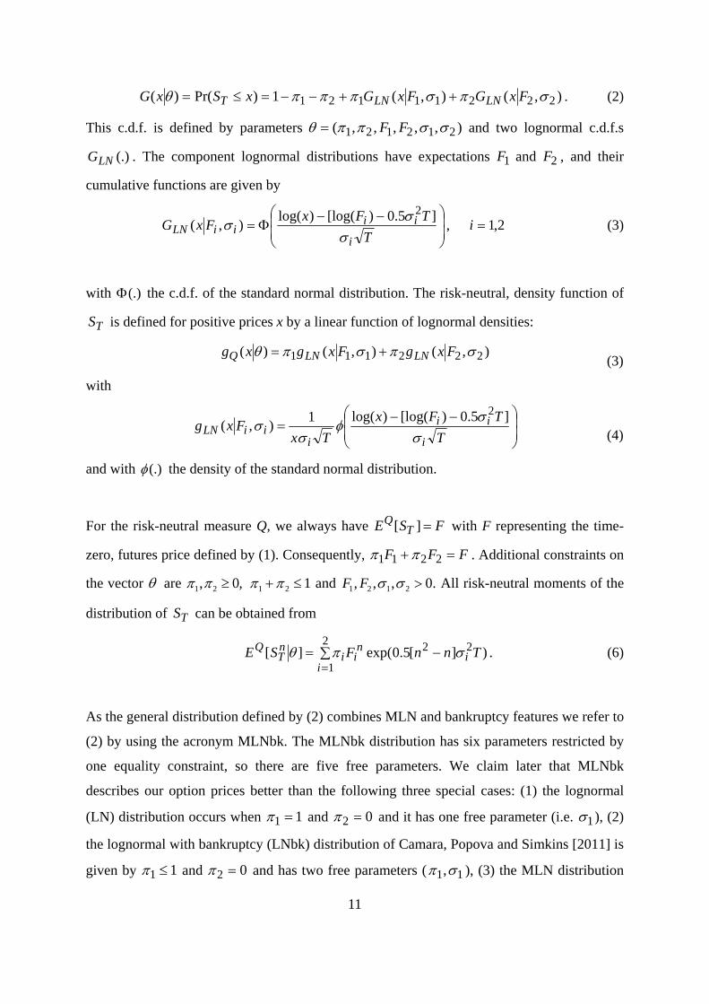
),(),(1)Pr()( 22211121 FxGFxGxSxG LNLNT . (2)

This c.d.f. is defined by parameters ),,,,,( 212121 FF and two lognormal c.d.f.s

(.)LNG . The component lognormal distributions have expectations 1F and 2F , and their

cumulative functions are given by

T

TFxFxG

i

iiiiLN

]5.0)[log()log(),(

2, 2,1i (3)

with (.) the c.d.f. of the standard normal distribution. The risk-neutral, density function of

TS is defined for positive prices x by a linear function of lognormal densities:

),(),()( 222111 FxgFxgxg LNLNQ (3)

with

T

TFx

TxFxg

i

ii

iiiLN

]5.0)[log()log(1),(

2

(4)

and with (.) the density of the standard normal distribution.

For the risk-neutral measure Q, we always have FSE TQ ][ with F representing the time-

zero, futures price defined by (1). Consequently, FFF 2211 . Additional constraints on

the vector are 1 2, 0, 1 2 1 and 1 2 1 2, , , 0.F F All risk-neutral moments of the

distribution of TS can be obtained from

)][5.0exp(][ 222

1TnnFSE i

ni

ii

nT

Q

. (6)

As the general distribution defined by (2) combines MLN and bankruptcy features we refer to

(2) by using the acronym MLNbk. The MLNbk distribution has six parameters restricted by

one equality constraint, so there are five free parameters. We claim later that MLNbk

describes our option prices better than the following three special cases: (1) the lognormal

(LN) distribution occurs when 11 and 02 and it has one free parameter (i.e. 1 ), (2)

the lognormal with bankruptcy (LNbk) distribution of Camara, Popova and Simkins [2011] is

given by 11 and 02 and has two free parameters ( 11, ), (3) the MLN distribution

12

excludes bankruptcy by requiring 121 and thus has four free parameters

( 2111 ,,, F ). Note that LNbk can be obtained as the special limiting case of MLN when

02 F and 2 is any fixed positive number. Consequently, we can state

MLNbk.MLNLNbkLN

Option pricing

European option prices are discounted, risk-neutral expectations of the option payoffs at

expiry. The Black [1976] pricing formula for European options on futures is simply an

application of risk-neutral pricing for a lognormal distribution, for which we represent call

and put prices respectively by the notation ),,,( TFXcB and ),,,( TFXpB ; here X is the

strike price, F is the time-zero futures price and is the annualized volatility. Therefore,

when the underlying asset price on the expiry date has a MLNbk distribution, at time 0 the

theoretical price of a call option is given by:

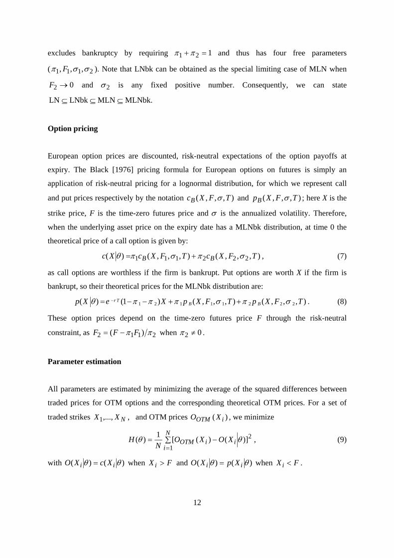
),,,(),,,()( 222111 TFXcTFXcXc BB , (7)

as call options are worthless if the firm is bankrupt. Put options are worth X if the firm is

bankrupt, so their theoretical prices for the MLNbk distribution are:

1 2 1 1 1 2 2 2( ) (1 ) ( , , , ) ( , , , )r TB Bp X e X p X F T p X F T . (8)

These option prices depend on the time-zero futures price F through the risk-neutral

constraint, as 2112 )( FFF when 02 .

Parameter estimation

All parameters are estimated by minimizing the average of the squared differences between

traded prices for OTM options and the corresponding theoretical OTM prices. For a set of

traded strikes NXX ,...,1 , and OTM prices )( iOTM XO , we minimize

2

1)]()([

1)( i

N

iiOTM XOXO

NH

, (9)

with )()( ii XcXO when FX i and )()( ii XpXO when FXi .

13

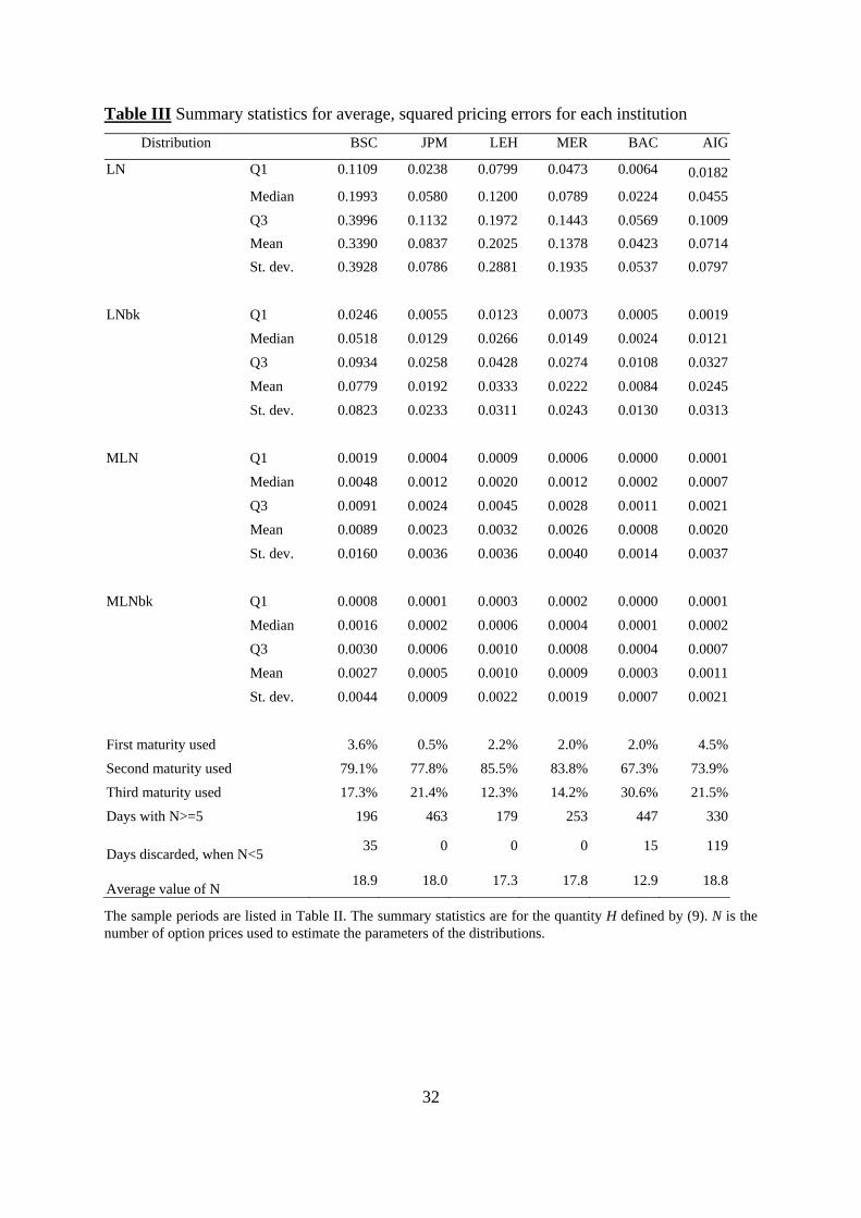
A summary of the parameter estimates obtained from the option prices included in our study

is provided by Tables III and IV. Table III summarises the values of H across the sample

periods. As the distributions of the H-values are positively skewed, we state results for both

means and medians. The LNbk distribution has two states (survive, with a lognormal

distribution, or go bankrupt) and it fits the option prices more accurately than a single

lognormal distribution. The median H for LNbk divided by the median H for LN varies from

11% to 27% across institutions; the ratio of means varies from 16% to 34%. However, the

LNbk distribution is simply a limiting case of the MLN distribution, which allows for two

general states. When we compare H-values for LNbk and MLN we find the more general

distribution has median values which are between 6% and 10% of the median values for the

special case; the ratios are 8% to 12% for mean values. The MLNbk distribution is our most

general specification and its values of H are a notable improvement upon all special cases.

The MLNbk distribution has medians which are between 19% and 37% of the MLN medians,

with mean ratios from 24% to 55%.

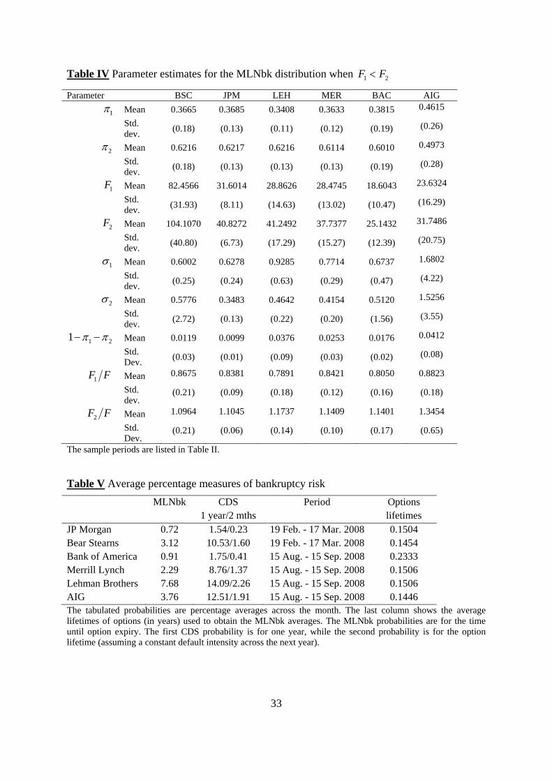
Table IV shows the means and standard deviations of the estimated parameters for the

MLNbk distribution. As is typical in the MLN literature for equity markets, the lower-

expectation state is less likely but more volatile, i.e. when 21 FF then 21 and

21 . The third state for MLNbk is seen to have a low average probability of bankruptcy

across each sample period, with 211 varying from 1.2% for BSC to 4.5% for AIG.

EMPIRICAL RESULTS

We first use option prices to compare the risk-neutral probability of bankruptcy for the six

financial institutions, contrasting the chances for acquiring, acquired, bankrupt and bailed-out

institutions. It is important to remember that all the probabilities are risk-neutral; they will

change if either real-world probabilities change or the market’s tolerance for risk changes.

Next, we compare the probabilities extracted from option prices with those implied by CDS

spreads. We find that similar information is revealed by the two sources. Finally, we provide

separate case studies for each institution, and discuss changes in risk-neutral bankruptcy

perceptions and densities especially when major relevant news items are announced.

14

Comparison of the probability of bankruptcy across institutions

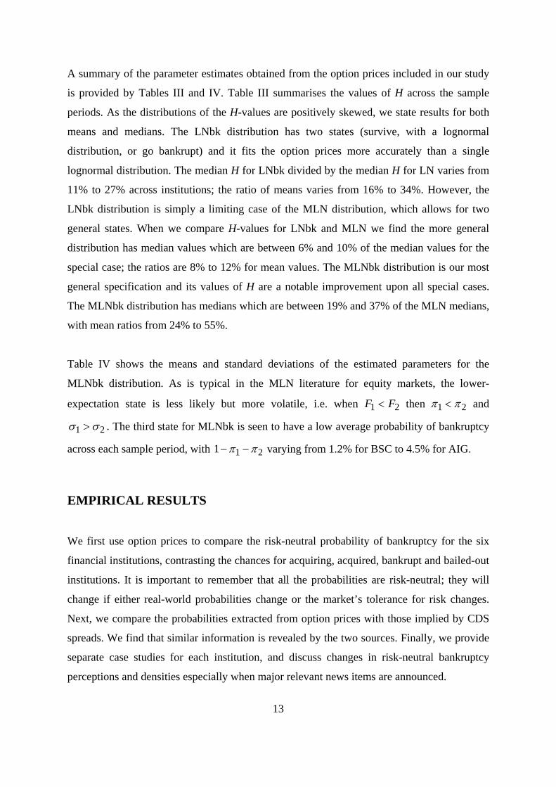
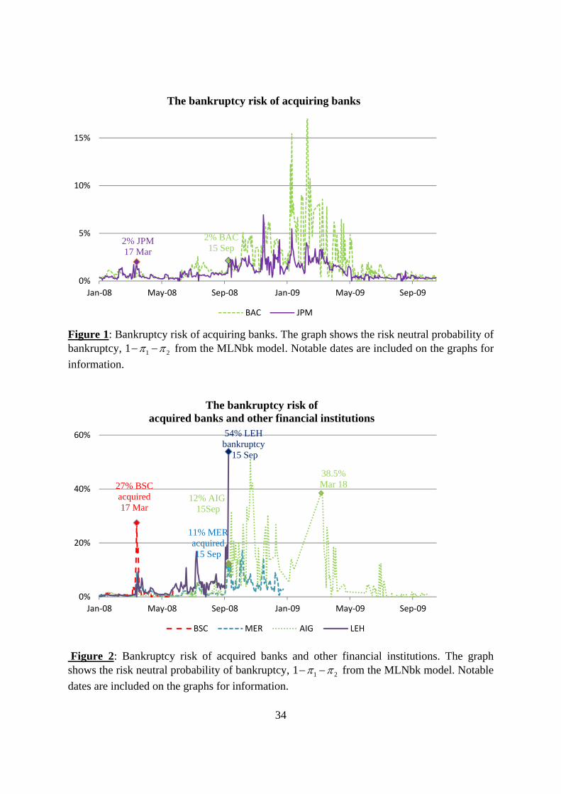
Figure 1 shows the bankruptcy probability for the two acquiring banks, JP Morgan and Bank

of America. The probability was less than 2% before September 20085. The probability of

bankruptcy around the Bear Stearns crisis in March 2008 was generally smaller than around

the Lehman Brothers failure in September 2008. The probabilities were relatively high from

September 2008 to June 2009, while in the second half of 2009 they decreased to less than

1%.

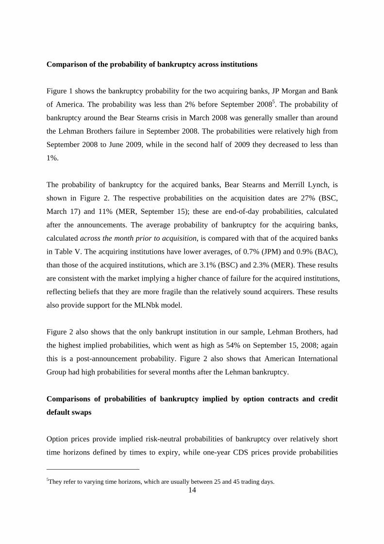
The probability of bankruptcy for the acquired banks, Bear Stearns and Merrill Lynch, is

shown in Figure 2. The respective probabilities on the acquisition dates are 27% (BSC,

March 17) and 11% (MER, September 15); these are end-of-day probabilities, calculated

after the announcements. The average probability of bankruptcy for the acquiring banks,

calculated across the month prior to acquisition, is compared with that of the acquired banks

in Table V. The acquiring institutions have lower averages, of 0.7% (JPM) and 0.9% (BAC),

than those of the acquired institutions, which are 3.1% (BSC) and 2.3% (MER). These results

are consistent with the market implying a higher chance of failure for the acquired institutions,

reflecting beliefs that they are more fragile than the relatively sound acquirers. These results

also provide support for the MLNbk model.

Figure 2 also shows that the only bankrupt institution in our sample, Lehman Brothers, had

the highest implied probabilities, which went as high as 54% on September 15, 2008; again

this is a post-announcement probability. Figure 2 also shows that American International

Group had high probabilities for several months after the Lehman bankruptcy.

Comparisons of probabilities of bankruptcy implied by option contracts and credit

default swaps

Option prices provide implied risk-neutral probabilities of bankruptcy over relatively short

time horizons defined by times to expiry, while one-year CDS prices provide probabilities

5They refer to varying time horizons, which are usually between 25 and 45 trading days.

15

over a one-year horizon. The two markets thus provide implied probabilities for different

horizons, in the same way that two-month and one-year interest rates and implied volatilities

provide two observations from the respective term structures.

Table V shows the probability of bankruptcy averages during one-month periods preceding

the key dates in March 2008 (for JP Morgan and Bear Stearns), and September 2008 (for the

other four institutions). We observe that the six probabilities rank in the same order for both

the options and CDS sources, so their rank correlation is one. This shows that the two sources

agreed about the relative bankruptcy risks. As the average option lifetimes are just under two

months it is not surprising that the option implied probabilities are smaller than the one-year

CDS probabilities. Table V also shows the equivalent CDS probabilities over option lifetimes,

after assuming a constant intensity for default for the next year. The option implied

probabilities are then seen to be larger than the CDS probabilities, by factors varying from

1.7 to 3.4. The higher option probabilities are consistent with a declining term structure of

bankruptcy risk; during a crisis we expect a higher chance of bankruptcy during the next two

months than during subsequent two-month periods.

A second comparison of option and CDS information can be attempted by asking if one

source leads the other in providing relevant information. Some evidence about relative timing

is given by finding the correlation between the bankruptcy chance on day t from options data

and the chance on day t from CDS prices, denoted by r . We find 101 rrr for three

institutions (JPM, BAC, AIG), while 101 rrr for two (BSC, MER) and 110 rrr for

one (LEH). We consider the evidence from these correlations to be inconclusive.

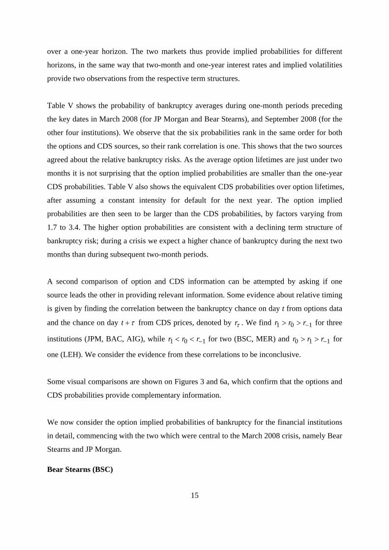
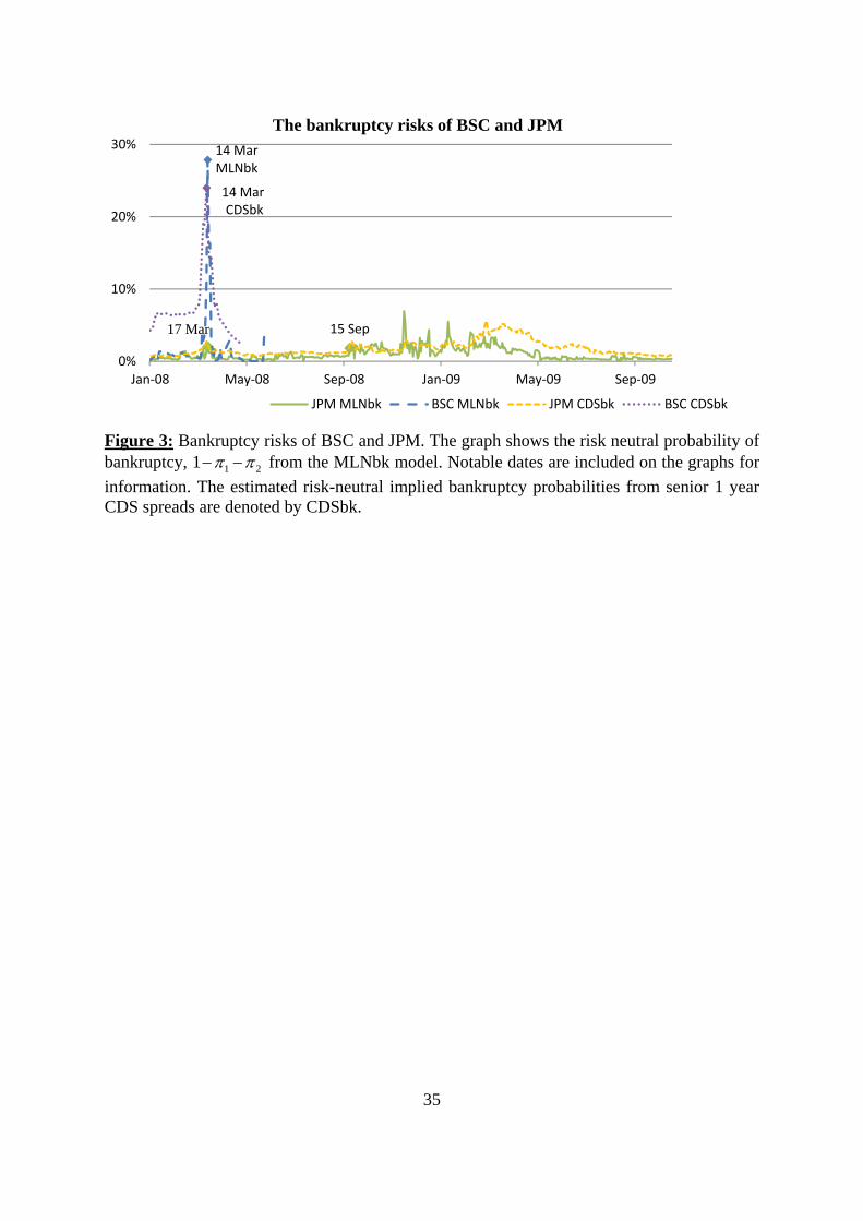
Some visual comparisons are shown on Figures 3 and 6a, which confirm that the options and

CDS probabilities provide complementary information.

We now consider the option implied probabilities of bankruptcy for the financial institutions

in detail, commencing with the two which were central to the March 2008 crisis, namely Bear

Stearns and JP Morgan.

Bear Stearns (BSC)

16

Figure 3 shows that BSC had a bankruptcy chance below 2% before Monday March 10. As

liquidity dried up, the probability increased reflecting rising fear among investors. On

Monday March 17, JP Morgan offered to acquire Bear Stearns at a low price when the

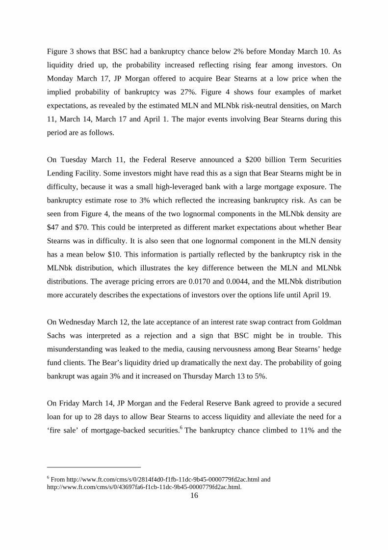
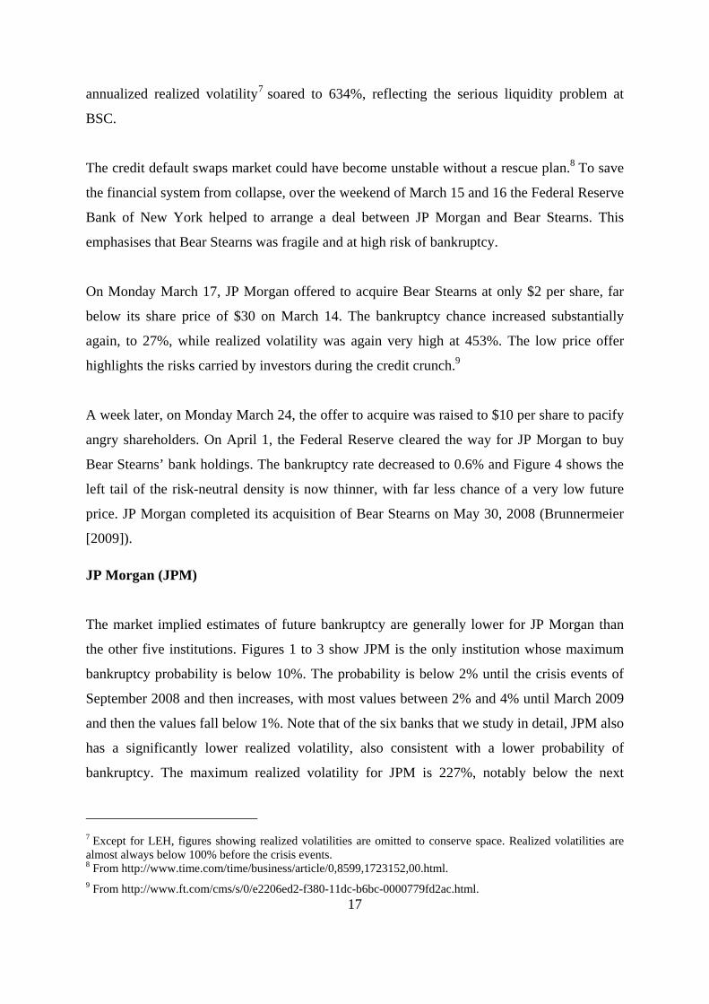
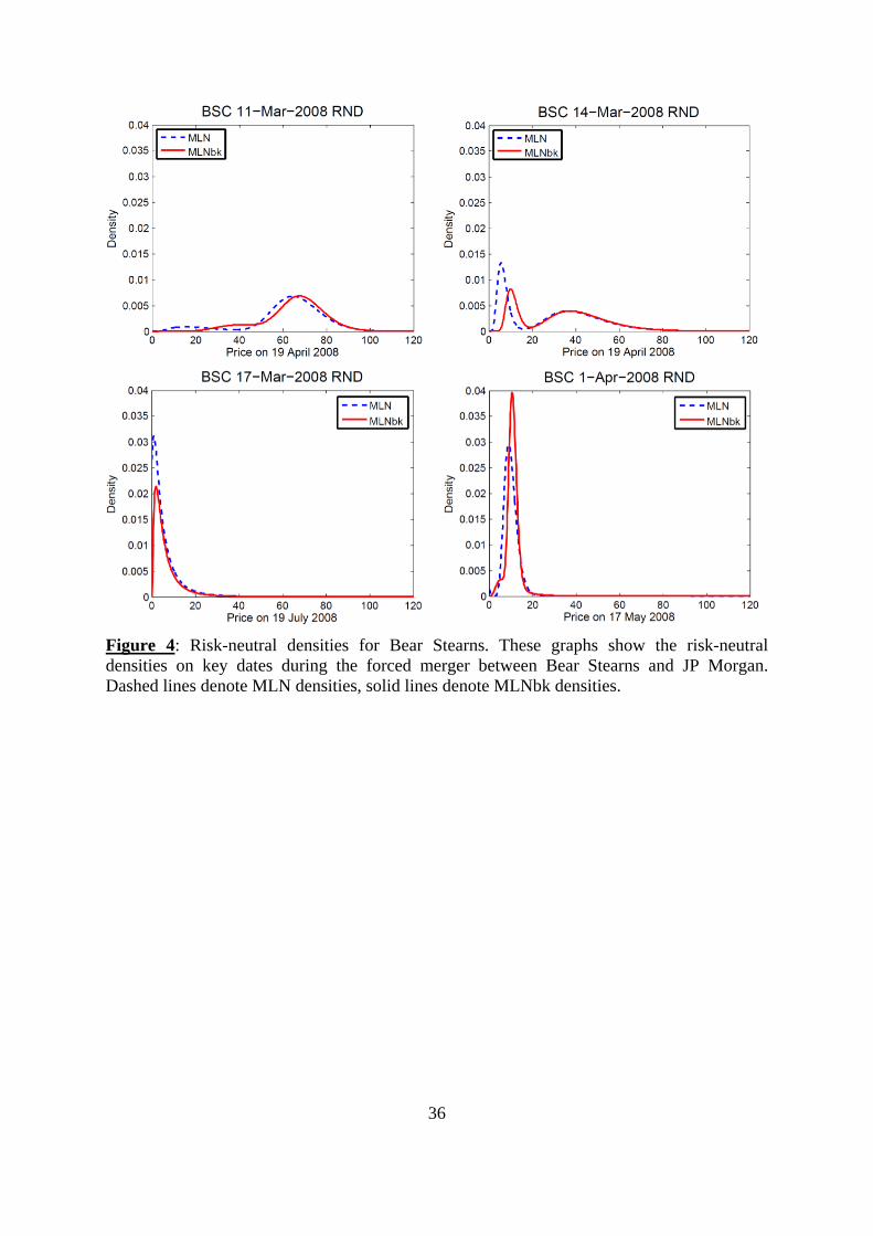
implied probability of bankruptcy was 27%. Figure 4 shows four examples of market

expectations, as revealed by the estimated MLN and MLNbk risk-neutral densities, on March

11, March 14, March 17 and April 1. The major events involving Bear Stearns during this

period are as follows.

On Tuesday March 11, the Federal Reserve announced a $200 billion Term Securities

Lending Facility. Some investors might have read this as a sign that Bear Stearns might be in

difficulty, because it was a small high-leveraged bank with a large mortgage exposure. The

bankruptcy estimate rose to 3% which reflected the increasing bankruptcy risk. As can be

seen from Figure 4, the means of the two lognormal components in the MLNbk density are

$47 and $70. This could be interpreted as different market expectations about whether Bear

Stearns was in difficulty. It is also seen that one lognormal component in the MLN density

has a mean below $10. This information is partially reflected by the bankruptcy risk in the

MLNbk distribution, which illustrates the key difference between the MLN and MLNbk

distributions. The average pricing errors are 0.0170 and 0.0044, and the MLNbk distribution

more accurately describes the expectations of investors over the options life until April 19.

On Wednesday March 12, the late acceptance of an interest rate swap contract from Goldman

Sachs was interpreted as a rejection and a sign that BSC might be in trouble. This

misunderstanding was leaked to the media, causing nervousness among Bear Stearns’ hedge

fund clients. The Bear’s liquidity dried up dramatically the next day. The probability of going

bankrupt was again 3% and it increased on Thursday March 13 to 5%.

On Friday March 14, JP Morgan and the Federal Reserve Bank agreed to provide a secured

loan for up to 28 days to allow Bear Stearns to access liquidity and alleviate the need for a

‘fire sale’ of mortgage-backed securities.6 The bankruptcy chance climbed to 11% and the

6 From http://www.ft.com/cms/s/0/2814f4d0-f1fb-11dc-9b45-0000779fd2ac.html and http://www.ft.com/cms/s/0/43697fa6-f1cb-11dc-9b45-0000779fd2ac.html.

17

annualized realized volatility7 soared to 634%, reflecting the serious liquidity problem at

BSC.

The credit default swaps market could have become unstable without a rescue plan.8 To save

the financial system from collapse, over the weekend of March 15 and 16 the Federal Reserve

Bank of New York helped to arrange a deal between JP Morgan and Bear Stearns. This

emphasises that Bear Stearns was fragile and at high risk of bankruptcy.

On Monday March 17, JP Morgan offered to acquire Bear Stearns at only $2 per share, far

below its share price of $30 on March 14. The bankruptcy chance increased substantially

again, to 27%, while realized volatility was again very high at 453%. The low price offer

highlights the risks carried by investors during the credit crunch.9

A week later, on Monday March 24, the offer to acquire was raised to $10 per share to pacify

angry shareholders. On April 1, the Federal Reserve cleared the way for JP Morgan to buy

Bear Stearns’ bank holdings. The bankruptcy rate decreased to 0.6% and Figure 4 shows the

left tail of the risk-neutral density is now thinner, with far less chance of a very low future

price. JP Morgan completed its acquisition of Bear Stearns on May 30, 2008 (Brunnermeier

[2009]).

JP Morgan (JPM)

The market implied estimates of future bankruptcy are generally lower for JP Morgan than

the other five institutions. Figures 1 to 3 show JPM is the only institution whose maximum

bankruptcy probability is below 10%. The probability is below 2% until the crisis events of

September 2008 and then increases, with most values between 2% and 4% until March 2009

and then the values fall below 1%. Note that of the six banks that we study in detail, JPM also

has a significantly lower realized volatility, also consistent with a lower probability of

bankruptcy. The maximum realized volatility for JPM is 227%, notably below the next

7 Except for LEH, figures showing realized volatilities are omitted to conserve space. Realized volatilities are almost always below 100% before the crisis events. 8 From http://www.time.com/time/business/article/0,8599,1723152,00.html. 9 From http://www.ft.com/cms/s/0/e2206ed2-f380-11dc-b6bc-0000779fd2ac.html.

18

highest which is 384% for MER. The average realized volatility for JPM is 55%, while over a

similar period including September, 2008, the next lowest is 67% for BAC10.

As already discussed, Bear Stearns was acquired by the relatively stable JPM in March 2008.

The estimated bankruptcy risk for JPM increased, temporarily, on March 17 to 2%. However,

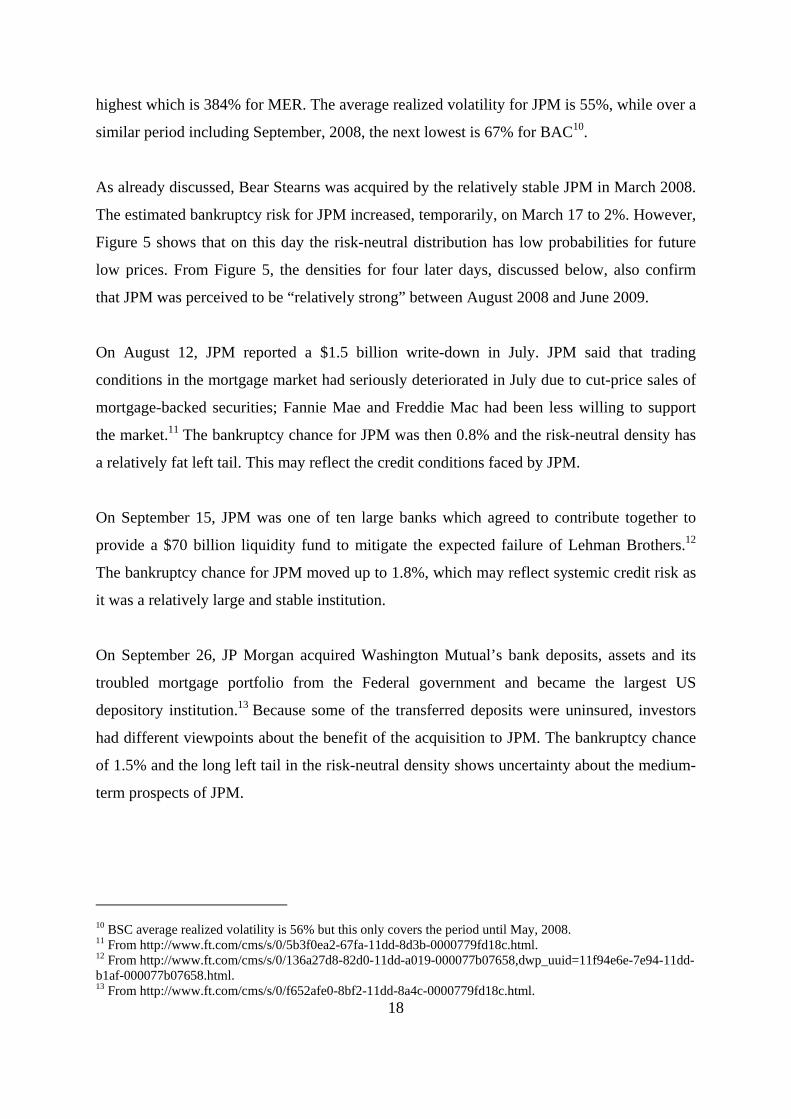
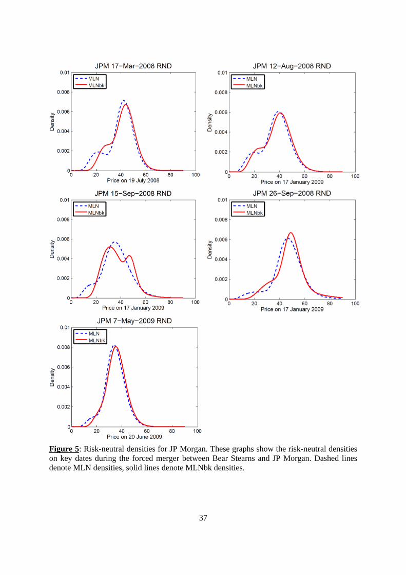
Figure 5 shows that on this day the risk-neutral distribution has low probabilities for future

low prices. From Figure 5, the densities for four later days, discussed below, also confirm

that JPM was perceived to be “relatively strong” between August 2008 and June 2009.

On August 12, JPM reported a $1.5 billion write-down in July. JPM said that trading

conditions in the mortgage market had seriously deteriorated in July due to cut-price sales of

mortgage-backed securities; Fannie Mae and Freddie Mac had been less willing to support

the market.11 The bankruptcy chance for JPM was then 0.8% and the risk-neutral density has

a relatively fat left tail. This may reflect the credit conditions faced by JPM.

On September 15, JPM was one of ten large banks which agreed to contribute together to

provide a $70 billion liquidity fund to mitigate the expected failure of Lehman Brothers.12

The bankruptcy chance for JPM moved up to 1.8%, which may reflect systemic credit risk as

it was a relatively large and stable institution.

On September 26, JP Morgan acquired Washington Mutual’s bank deposits, assets and its

troubled mortgage portfolio from the Federal government and became the largest US

depository institution.13 Because some of the transferred deposits were uninsured, investors

had different viewpoints about the benefit of the acquisition to JPM. The bankruptcy chance

of 1.5% and the long left tail in the risk-neutral density shows uncertainty about the medium-

term prospects of JPM.

10 BSC average realized volatility is 56% but this only covers the period until May, 2008. 11 From http://www.ft.com/cms/s/0/5b3f0ea2-67fa-11dd-8d3b-0000779fd18c.html. 12 From http://www.ft.com/cms/s/0/136a27d8-82d0-11dd-a019-000077b07658,dwp_uuid=11f94e6e-7e94-11dd-b1af-000077b07658.html. 13 From http://www.ft.com/cms/s/0/f652afe0-8bf2-11dd-8a4c-0000779fd18c.html.

19

On May 7, 2009, a stress test by the government showed that JPM was adequately capitalized

and was more able to repay bailout dollars than its peers.14 The announcement of the test

result should have reassured investors and the bankruptcy chance fell to 0.6%. The

pronounced left tail, seen in previous risk-neutral densities, disappears and the density

becomes almost symmetric. This indicates that the market had few concerns about JP Morgan

surviving the liquidity crisis.

Lehman Brothers (LEH)

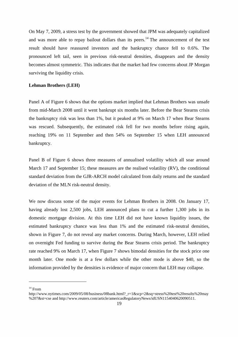
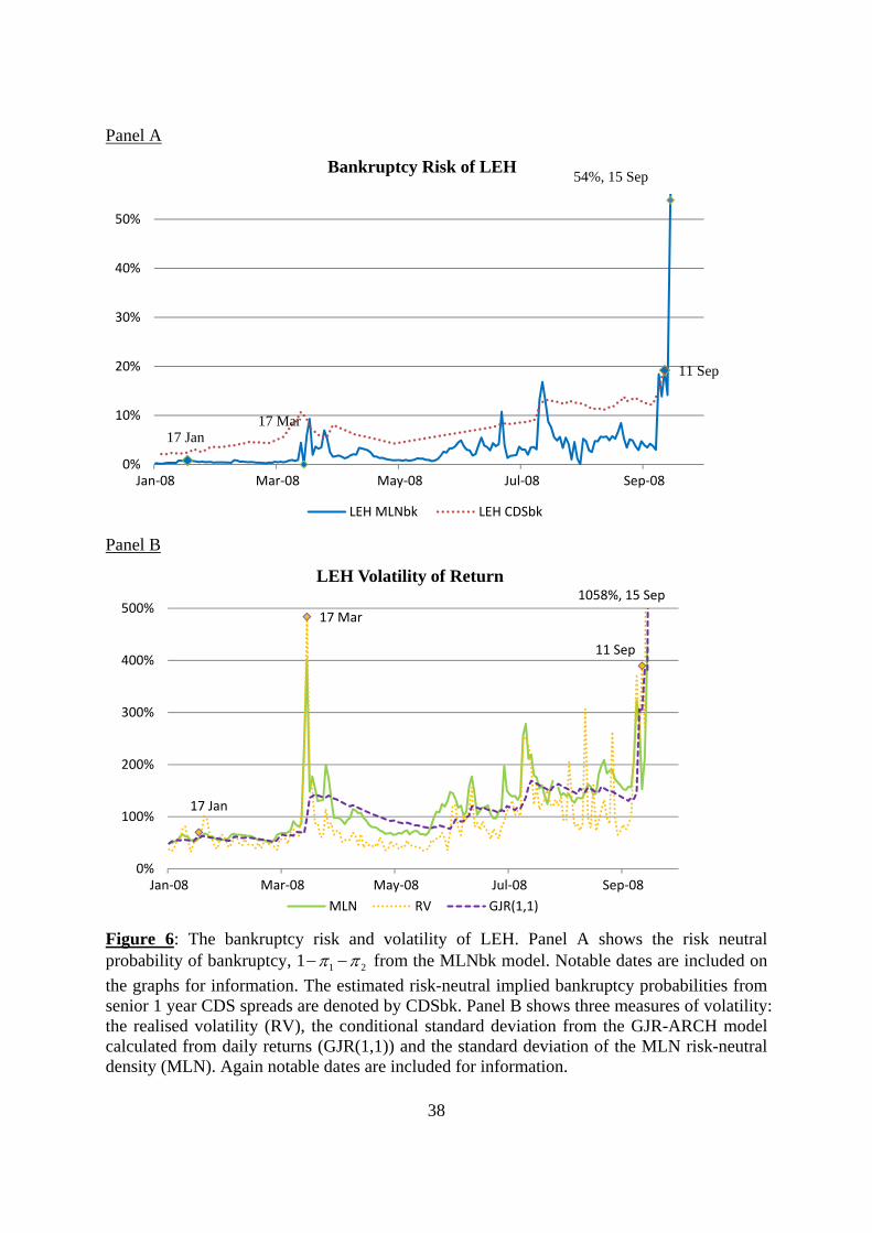
Panel A of Figure 6 shows that the options market implied that Lehman Brothers was unsafe

from mid-March 2008 until it went bankrupt six months later. Before the Bear Stearns crisis

the bankruptcy risk was less than 1%, but it peaked at 9% on March 17 when Bear Stearns

was rescued. Subsequently, the estimated risk fell for two months before rising again,

reaching 19% on 11 September and then 54% on September 15 when LEH announced

bankruptcy.

Panel B of Figure 6 shows three measures of annualised volatility which all soar around

March 17 and September 15; these measures are the realised volatility (RV), the conditional

standard deviation from the GJR-ARCH model calculated from daily returns and the standard

deviation of the MLN risk-neutral density.

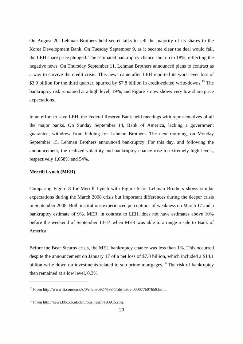
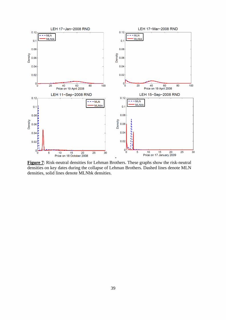
We now discuss some of the major events for Lehman Brothers in 2008. On January 17,

having already lost 2,500 jobs, LEH announced plans to cut a further 1,300 jobs in its

domestic mortgage division. At this time LEH did not have known liquidity issues, the

estimated bankruptcy chance was less than 1% and the estimated risk-neutral densities,

shown in Figure 7, do not reveal any market concerns. During March, however, LEH relied

on overnight Fed funding to survive during the Bear Stearns crisis period. The bankruptcy

rate reached 9% on March 17, when Figure 7 shows bimodal densities for the stock price one

month later. One mode is at a few dollars while the other mode is above $40, so the

information provided by the densities is evidence of major concern that LEH may collapse.

14 From http://www.nytimes.com/2009/05/08/business/08bank.html?_r=1&scp=2&sq=stress%20test%20results%20may%207&st=cse and http://www.reuters.com/article/americasRegulatoryNews/idUSN1154040620090511.

20

On August 20, Lehman Brothers held secret talks to sell the majority of its shares to the

Korea Development Bank. On Tuesday September 9, as it became clear the deal would fail,

the LEH share price plunged. The estimated bankruptcy chance shot up to 18%, reflecting the

negative news. On Thursday September 11, Lehman Brothers announced plans to contract as

a way to survive the credit crisis. This news came after LEH reported its worst ever loss of

$3.9 billion for the third quarter, spurred by $7.8 billion in credit-related write-downs.15 The

bankruptcy risk remained at a high level, 19%, and Figure 7 now shows very low share price

expectations.

In an effort to save LEH, the Federal Reserve Bank held meetings with representatives of all

the major banks. On Sunday September 14, Bank of America, lacking a government

guarantee, withdrew from bidding for Lehman Brothers. The next morning, on Monday

September 15, Lehman Brothers announced bankruptcy. For this day, and following the

announcement, the realized volatility and bankruptcy chance rose to extremely high levels,

respectively 1,058% and 54%.

Merrill Lynch (MER)

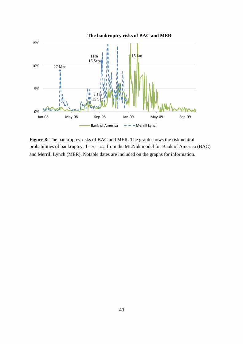
Comparing Figure 8 for Merrill Lynch with Figure 6 for Lehman Brothers shows similar

expectations during the March 2008 crisis but important differences during the deeper crisis

in September 2008. Both institutions experienced perceptions of weakness on March 17 and a

bankruptcy estimate of 9%. MER, in contrast to LEH, does not have estimates above 10%

before the weekend of September 13-14 when MER was able to arrange a sale to Bank of

America.

Before the Bear Stearns crisis, the MEL bankruptcy chance was less than 1%. This occurred

despite the announcement on January 17 of a net loss of $7.8 billion, which included a $14.1

billion write-down on investments related to sub-prime mortgages.16 The risk of bankruptcy

then remained at a low level, 0.3%.

15 From http://www.ft.com/cms/s/0/c4cb3b92-7f98-11dd-a3da-000077b07658.html.

16 From http://news.bbc.co.uk/2/hi/business/7193915.stm.

21

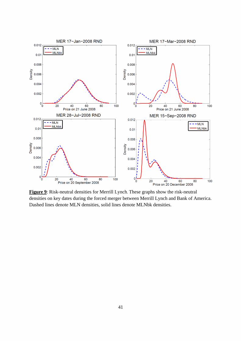
Later, on July 28, Merrill Lynch announced a $8.5 billion share offer and a $5.7 billion fire

sale of toxic mortgage securities.17 The share return on this day was -12% and the probability

of bankruptcy increased to 2.3%.

On Sunday September 14, as its competitor Lehman Brothers was sinking, Merrill Lynch

“reading the signs … announced … that it had sold itself to Bank of America for $50 billion”

(Brunnermeier [2009]). This price was equivalent to $29 per share, which was 70% higher

than Merrill’s most recent traded stock price. The realized volatility and bankruptcy chance

on Monday September 15 were 172% and 11% respectively. The relatively high probability

of future bankruptcy on this and subsequent days may reflect a lack of confidence either in

the sale of MEL or in the strength of its rescuer. Figure 9 shows the estimated risk-neutral

densities on September 15 are highly skewed to the left, with expectations far below $29.

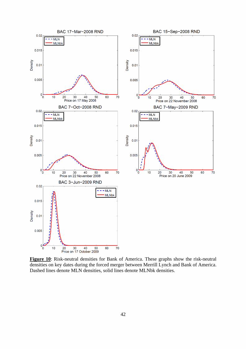
Bank of America (BAC)

As shown by Figures 1 and 8, the market considered Bank of America to be relatively safe

during the crises of March and September 2008, but less safe after these crises. The estimated

probability of bankruptcy is 2% on September 15 and it is lower before then. There are

several estimates around 5% later in 2008. These are followed by some estimates above 10%

during the first half of 2009 and by much lower values later in the year. The five examples of

BAC risk-neutral densities on Figure 10 show expectations falling as time progresses,

because the share price falls, but they do not show high chances of very low prices in the

future.

On Saturday September 13, Bank of America was seen as the leading contender to buy

Lehman Brothers, but the US government was reluctant to provide public backing for a take-

over.18 On Sunday September 14, Bank of America instead agreed to acquire Merrill Lynch.19

The inferred probability of bankruptcy for BAC on Monday September 15 increased, but only

to 2.1%, which reflects some level of systemic credit risk following the LEH bankruptcy.

17 From http://www.ft.com/cms/s/0/3bf7930e-5cf4-11dd-8d38-000077b07658.html. 18 From http://www.ft.com/cms/s/0/306f879c-812c-11dd-82dd-000077b07658.html. 19 From http://www.ft.com/cms/s/0/0ba5fbd8-82a0-11dd-a019-000077b07658,dwp_uuid=11f94e6e-7e94-11dd-b1af-000077b07658.html.

22

On October 7, Bank of America reported its third quarter earnings which were less than

analysts’ expectations. BAC said it would raise $10 billion of capital and cut its dividend in

order to get through the credit crisis.20 The immediate response to the negative news was a

one-day return of -30%.

On October 14, the US government injected $250 billion into the US banking system. As part

of their plan, BAC was to get $25 billion in government funds. In return, the government

would take an equity position in the bank. 21 While the one-day return was 15%, the

probability of bankruptcy went to 3.3%. Thus market concerns about another bankruptcy

were not eliminated by the injection announcement.

On Saturday December 20, S&P downgraded the ratings of six major US banks reflecting

anxieties that financial crisis could be longer and deeper than previously expected. Bank of

America’s acquisition of Merrill Lynch raised concerns, because MEL could generate more

write-downs in commercial real estate and leveraged loans.22 On Monday December 22, the

bankruptcy estimate was 1.9%.

On January 15, 2009, BAC received a $138 billion bailout. The bailout was to be used to

improve the balance sheet at the newly acquired MEL and to guarantee potential losses on

‘toxic assets’.23 The BAC share price fell 20% on the day and the estimated probability of

bankruptcy climbed to a new high level, of 12%. This clearly shows that market concerns

were not alleviated by the bailout announcement.

By May the bankruptcy estimates were falling. Nevertheless, on May 7, stress test results

exposed Bank of America’s lack of capital to survive worst-case scenarios. The bankruptcy

estimate was then 2.3%, compared with 0.6% for JP Morgan which was reported to be

adequately capitalized. On May 20, BAC sold shares to raise $13.5 billion, which represented

considerable progress towards meeting its capital-raising requirement. On June 3, US banks

20 From http://www.ft.com/cms/s/0/50592a82-93fa-11dd-b277-0000779fd18c.html. 21 From http://www.ft.com/cms/s/0/395a0fa6-99f2-11dd-960e-000077b07658.html. 22 From http://www.ft.com/cms/s/0/8b20cc34-ce37-11dd-8b30-000077b07658.html. 23 From http://www.ft.com/cms/s/0/7ebeb6b0-e35c-11dd-a5cf-0000779fd2ac.html.

23

sold common shares and non-guaranteed debt to raise more money than required by

regulators. Mutual funds and other large institutional investors bought shares aggressively

and stock prices reflected the improving situation. BAC shares went up by 263% from

March’s low point, while JPM was up 118%.24 With the improvement in liquidity conditions,

the realized volatility and bankruptcy estimate decreased to 40% and 0.4%, respectively. The

market gradually reverted to more normal conditions and the bankruptcy estimate was close

to zero after August 2009.

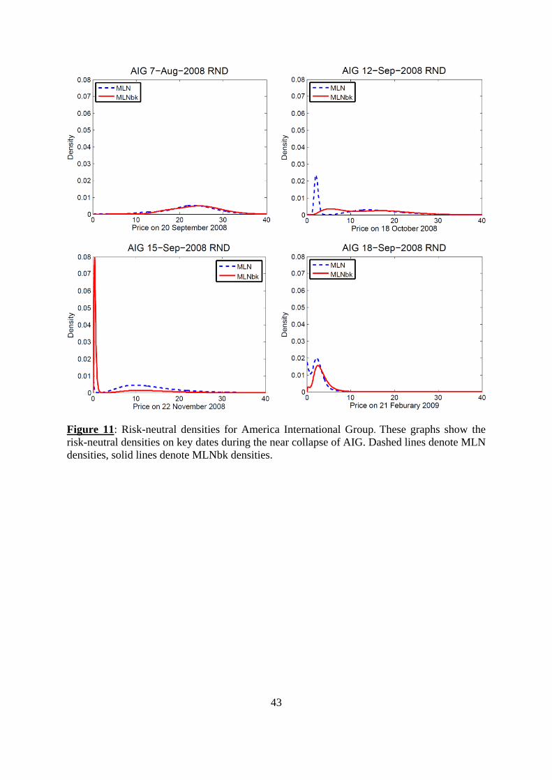
American International Group (AIG)

As can be seen from Figures 1 and 2, AIG is the only financial institution in our sample to

have several bankruptcy estimates above 20%, all of which occurred during 2008 after

September 11. AIG was active in the derivatives business, including credit default swaps,

which insure against corporate default. It was severely affected by the liquidity dry-up during

the financial crisis. AIG received government bailouts between September 2008 and March

2009 and consequently survived the financial crisis. Afterwards its implied probability of

bankruptcy stayed low, and close to zero after August 2009.

The estimated chance of bankruptcy is less than 3% in the first half of 2008, and increases

after July 2008. On 7 August 2008, AIG announced a higher than expected loss for large

subprime write-downs. The bankruptcy chance was then less than 1.5%. The slightly fat left

tails of the risk-neutral densities in Figure 11 reflect concerns that AIG might perform worse

in the near future.

On Friday September 12, S&P put AIG on a negative credit watch, signaling a possible rating

cut. The bankruptcy chance and realized volatility were 13.5% and 23.8%. On Monday

September 15, AIG made a deal with the New York insurance regulators to add liquidity.

Despite the deal, all the major rating agencies downgraded AIG’s long-term credit rating to

reflect its losses from mortgage-related investments and credit derivatives.25 Its share price

reflected the shock of the credit downgrades and the dramatic news about LEH and MER. 24 From http://online.wsj.com/article/SB124398503075879165.html. 25 From http://www.ft.com/cms/s/0/abaf3dee-834d-11dd-907e-000077b07658,dwp_uuid=11f94e6e-7e94-11dd-b1af-000077b07658.html

24

The daily return (change in the price logarithm) from Friday’s close to Monday’s close was -

93%. Panic is also shown by the very high realized volatility of 828%, and the bankruptcy

risk estimate of 12%. The high volatility can be seen in Figure 11 which shows the fat tails of

the risk neutral densities on September 12 and 15.

On September 16, the Federal Reserve announced that it would lend AIG $85 billion in

emergency funds in return for an 80% controlling stake. The implementation of a government

stake was to prevent existing shareholders from taking advantage of a bailout. 26 The

exceptionally high realized volatility of 1,237% and the bankruptcy risk of 11% indicate

heightened fear about future uncertainty.

On September 18, the world’s major central banks announced an injection of $180 billion to

improve liquidity. This action led to a decrease in overnight interbank lending. But the

continuing increase in longer-term interbank lending rates indicated that liquidity among

banks remained suspect.27 The AIG return was 27%, and the realized volatility estimate

decreased to 236%. This decrease reflects the positive features of the central bank actions,

although strong concerns remain as the probability of bankruptcy increased to 22% on

September 18.

By October 24, AIG had borrowed three-quarters of the rescue fund set up by the government.

The money was used to write down the bad debts which AIG guaranteed for other firms’

risky mortgage investments. The new CEO of AIG warned that the $123 billion fund

provided by the government might not be enough to keep AIG afloat.28 Investors read this as

a negative signal and the return was -21%. The bankruptcy chance was then very high at 35%.

On Sunday November 9, AIG received a $150 billion government bailout to reduce interest

payments and provide more time to sell assets.29 The bankruptcy risk decreased to 3% on the

next day.

26 From http://www.ft.com/cms/s/0/271257f2-83f1-11dd-bf00-000077b07658.html. 27 From http://www.ft.com/cms/s/0/e91b24b6-8557-11dd-a1ac-0000779fd18c.html. 28 From http://www.washingtonpost.com/wp-dyn/content/article/2008/10/23/AR2008102303352.html. 29 From http://www.ft.com/cms/s/0/614586b4-ae9f-11dd-b621-000077b07658.html.

25

On March 2, 2009, AIG announced a fourth quarter loss of $61.7 billion, around $23 per

share, most of which stemmed from write-downs of credit default swaps and debt. AIG could

access $30 billion of new government capital and this prevented AIG from credit

downgrades.30 After two weeks, the bankruptcy risk for AIG gradually decreased and stayed

at a low level.

CONCLUSIONS

We have developed a risk-neutral density model that uses options prices and estimates the

chance of bankruptcy under a risk-neutral measure. The MLNbk model extracts RNDs more

accurately than other RND models including a standard mixture of lognormals and a

lognormal with a bankruptcy term. The resulting density shows the market expectation of

stock prices over the lifetime of the options as well as the probability of bankruptcy over the

remaining lifetime of the options. This information is forward looking, allowing investors and

risk managers the possibility to estimate the chances of future bankruptcies.

We analyze in detail six major banks during the financial crisis period. As expected, when

considering the forced merger cases we find a higher chance of bankruptcy for the acquired

bank than for the acquiring bank. From analysis of the banks through key days in the

financial crisis we see how the RND and probability of bankruptcy responds to news. We see

that news announcements can have a significant effect on future bankruptcy probabilities as

well as changing the shape of the RND. These case studies show in detail the information that

can be obtained from option prices using the MLNbk model.

Finally, credit default swap prices provide similar and complementary information about risk-

neutral perceptions of extreme future outcomes. Our RND models provide probabilities over

short horizons, typically two months, in contrast to CDS probabilities for a year or more. We

find that annualized measures of bankruptcy or default probabilities are higher from option

30 From http://www.reuters.com/article/GCA-CreditCrisis/idUSN0134457520090303.

26

prices during the financial crisis, reflecting that any default is more likely in the next month

or two than further into the future.

27

REFERENCES

Agarwal, V. and R. Taffler. “Comparing the performance of market-based and accounting-

based bankruptcy prediction models.” Journal of Banking and Finance, 32 (2008), 1541-

1551.

Allen, F. and E. Carletti. “The role of liquidity in financial crises.” 2008 Jackson Hole

conference proceedings, Federal Reserve Bank of Kansas City (2008), 379-412.

Altman, E. “Financial ratio, discriminant analysis, and the prediction of corporate

bankruptcy.” Journal of Finance, 23 (1968), 589-609.

Amel, D., C. Barnes, F. Panetta and C. Salleo. “Consolidation and efficiency in the financial

sector: A review of the international evidence.” Journal of Banking and Finance, 28 (2004),

2493-2519.

Amel-Zadeh, A. and G. Meeks. Bank failure, mark-to-market, and thefinancial crisis. Abacus,

2011.

Bharath, S. and T. Shumway. “Forecasting default with the Merton distance to default model.”

Review of Financial Studies, 21 (2008), 1339-1369.

Birru, J. and S. Figlewski. “Anatomy of a meltdown: The risk neutral density for the S&P

500 in the fall of 2008.” Journal of Financial Markets, 15 (2012), 151-180.

Black, F. “The pricing of commodity contracts.” Journal of Financial Economics, 3 (1976),

167-179.

Bliss, R.R. and N. Panigirtzoglou. “Testing the stability of implied probability density

functions.” Journal of Banking and Finance, 26 (2002), 381-422.

28

Brigo, D. and F. Mercurio. Lognormal-mixture dynamics and calibration to market volatility

smiles. International Journal of Theoretical and Applied Finance, 5 (2002), 427-446.

Brunnermeier, M. “Deciphering the liquidity and credit crunch 2007-08.” Journal of

Economic Perspectives, 23 (2009), 77-100.

Camara, A., I. Popova and B. Simkins. “A compatative study of the probability of default for

global financial firms.” Journal of Banking and Finance, 36 (2011), 717-732.

Chen, Z. and W. Fong. “Was the writing on the wall? an options analysis of the 2008 Lehman

Brothers crisis.” Journal of Investment Management, 10 (2012), 1-12.

Fabozzi, F., R.-R. Chen, S.-Y. Hu, and G.-G. Pan. “Tests of the performance of structural

models in bankruptcy prediction.” Journal of Credit Risk, 6 (2010), 37-78.

Figlewski, S. “Estimating the implied risk neutral density for the U.S. market portfolio.” In

Bollerslev, T., Russell, J., Watson, M. (eds.), Volatility and Time Series Econometrics:

Essays in Honor of Robert F. Engle. Oxford, UK: Oxford University Press, 2009.

Focarelli, D., F. Panetta and C. Salleo. “Why do banks merge?” Journal of Money, Credit,

and Banking, 34 (2002), 1047-1066.

Hillegeist, S., E. Keating, D. Cram and K. Lundstedt. “Assessing the probability of

bankruptcy.” Review of Accounting Studies, 9 (2004), 5-34.

Jankowitsch, R., F. Nagler and M.G. Subrahmanyam. “The determinants of recovery rates in

the US corporate bond market.” Journal of Financial Economics (2014), forthcoming.

Jondeau, E. and M. Rockinger. “Reading the smile: the message conveyed by methods which

infer risk neutral densities.” Journal of International Money and Finance, 19 (2000), 885-915.

Liu, X., M.B. Shackleton, S.J. Taylor and X. Xu. “Closed-form transformations from risk-

neutral to real-world distributions.” Journal of Banking and Finance, 31 (2007), 1501-1520.

29

Malz, A.M. “Estimating the probability distribution of the future exchange rate from option

prices.” Journal of Derivatives, 5 (1997a), 18-36.

Malz, A.M. “Option-implied probability distributions and currency excess returns.” Staff

Reports, 32 (1997b), Federal Reserve Bank of New York.

Melick, W.R. and C.P. Thomas. “Recovering an asset's implied PDF from option prices: An

application to crude oil during the Gulf crisis.” Journal of Financial and Quantative Analysis,

32 (1997), 91-115.

Merton, R.C. “On the pricing of corporate debt: The risk structure of interest rates.” Journal

of Finance, 29 (1974), 449-470.

Petersen, M. and R. Rajan. “Does distance still matter? The information revolution in small

business lending.” Journal of Finance, 57 (2002), 2533-2570.

Poon, S.-H. and C.W.J. Granger. “Forecasting volatility in financial markets: A review.”

Journal of Economic Literature, 41 (2003), 478-539.

Rhee, R. “Case study of the merger between Bank of America and Merrill Lynch.” Working

paper, University of Maryland Legal Studies, 2010.

Ritchey, R.J. “Call option valuation for discrete normal mixtures.” Journal of Financial

Research, 13 (1990), 285-296.

Sarbu, S., C. Schmitt and M. Uhrig-Homburg. “Market expectations of recovery rates.”

Working paper, Karlsruhe Institute of Technology, 2013.

Shackleton, M.B., S.J. Taylor and P. Yu. “A multi-horizon comparison of density forecasts

for the S&P 500 using index returns and option prices.” Journal of Banking and Finance, 34

(2010), 2678-2693.

30

Shumway, T. “Forecasting bankruptcy more accurately: A simple hazard model.” Journal of

Business, 74 (2001), 101-124.

Taylor, S.J. Asset Price Dynamics, Volatility, and Prediction. Princeton, NJ: Princeton

University Press, 2005.

Taylor, S.J., P.K. Yadav and Y. Zhang. “Cross-sectional analysis of risk-neutral skewness.”

Journal of Derivatives, 16 (2009), 38-53.

Zmijewski, M. “Methodological issues related to the estimation of financial distress

prediction models.” Journal of Accounting Research, 22 (1984), 59-82.

31

TABLES AND FIGURES

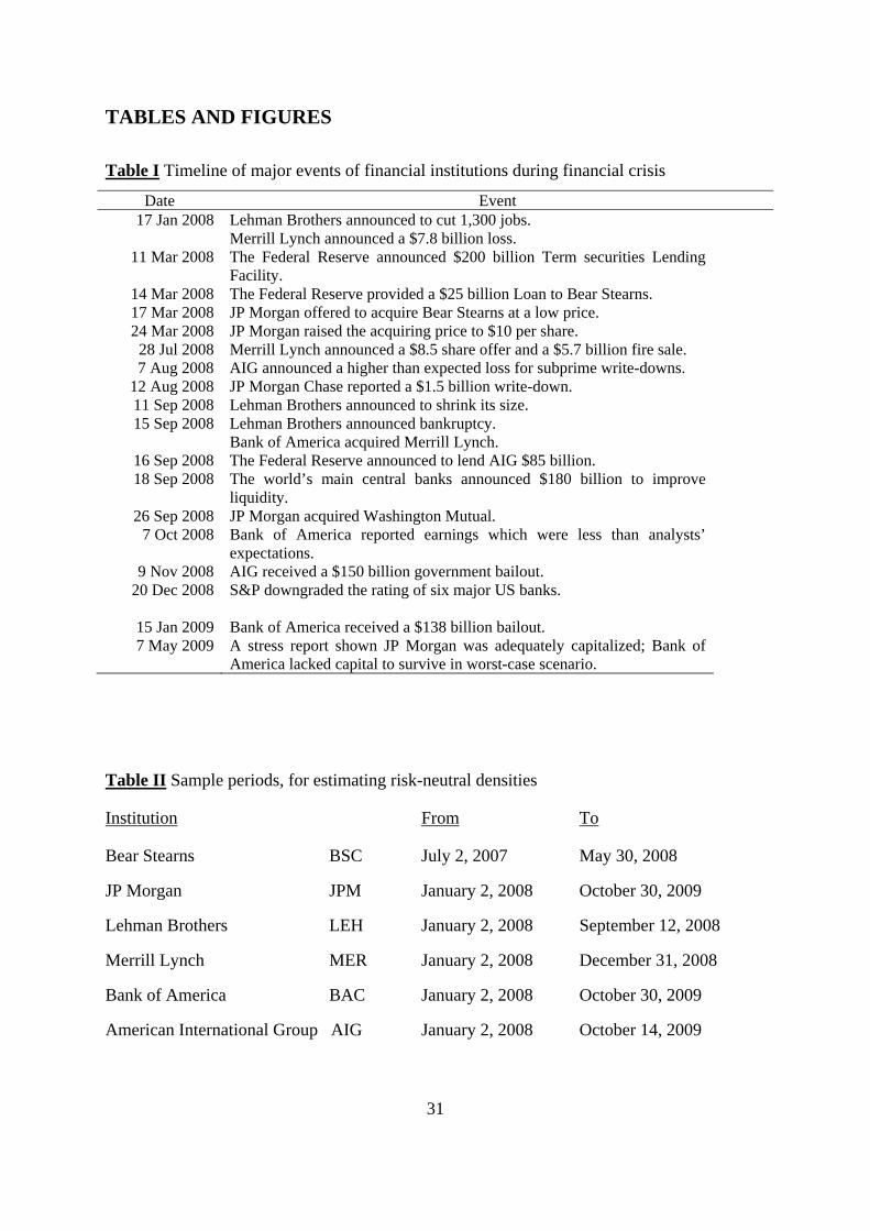
Table I Timeline of major events of financial institutions during financial crisis

Date Event 17 Jan 2008 Lehman Brothers announced to cut 1,300 jobs.

Merrill Lynch announced a $7.8 billion loss. 11 Mar 2008 The Federal Reserve announced $200 billion Term securities Lending

Facility. 14 Mar 2008 The Federal Reserve provided a $25 billion Loan to Bear Stearns. 17 Mar 2008 JP Morgan offered to acquire Bear Stearns at a low price. 24 Mar 2008 JP Morgan raised the acquiring price to $10 per share. 28 Jul 2008 Merrill Lynch announced a $8.5 share offer and a $5.7 billion fire sale. 7 Aug 2008 AIG announced a higher than expected loss for subprime write-downs.

12 Aug 2008 JP Morgan Chase reported a $1.5 billion write-down. 11 Sep 2008 Lehman Brothers announced to shrink its size. 15 Sep 2008 Lehman Brothers announced bankruptcy.

Bank of America acquired Merrill Lynch. 16 Sep 2008 The Federal Reserve announced to lend AIG $85 billion. 18 Sep 2008 The world’s main central banks announced $180 billion to improve

liquidity. 26 Sep 2008 JP Morgan acquired Washington Mutual.

7 Oct 2008 Bank of America reported earnings which were less than analysts’ expectations.

9 Nov 2008 AIG received a $150 billion government bailout. 20 Dec 2008 S&P downgraded the rating of six major US banks.

15 Jan 2009 Bank of America received a $138 billion bailout. 7 May 2009 A stress report shown JP Morgan was adequately capitalized; Bank of

America lacked capital to survive in worst-case scenario.

Table II Sample periods, for estimating risk-neutral densities

Institution From To

Bear Stearns BSC July 2, 2007 May 30, 2008

JP Morgan JPM January 2, 2008 October 30, 2009

Lehman Brothers LEH January 2, 2008 September 12, 2008

Merrill Lynch MER January 2, 2008 December 31, 2008

Bank of America BAC January 2, 2008 October 30, 2009

American International Group AIG January 2, 2008 October 14, 2009

32

Table III Summary statistics for average, squared pricing errors for each institution

Distribution BSC JPM LEH MER BAC AIG

LN Q1 0.1109 0.0238 0.0799 0.0473 0.0064 0.0182

Median 0.1993 0.0580 0.1200 0.0789 0.0224 0.0455

Q3 0.3996 0.1132 0.1972 0.1443 0.0569 0.1009

Mean 0.3390 0.0837 0.2025 0.1378 0.0423 0.0714

St. dev. 0.3928 0.0786 0.2881 0.1935 0.0537 0.0797

LNbk Q1 0.0246 0.0055 0.0123 0.0073 0.0005 0.0019

Median 0.0518 0.0129 0.0266 0.0149 0.0024 0.0121

Q3 0.0934 0.0258 0.0428 0.0274 0.0108 0.0327

Mean 0.0779 0.0192 0.0333 0.0222 0.0084 0.0245

St. dev. 0.0823 0.0233 0.0311 0.0243 0.0130 0.0313

MLN Q1 0.0019 0.0004 0.0009 0.0006 0.0000 0.0001

Median 0.0048 0.0012 0.0020 0.0012 0.0002 0.0007

Q3 0.0091 0.0024 0.0045 0.0028 0.0011 0.0021

Mean 0.0089 0.0023 0.0032 0.0026 0.0008 0.0020

St. dev. 0.0160 0.0036 0.0036 0.0040 0.0014 0.0037

MLNbk Q1 0.0008 0.0001 0.0003 0.0002 0.0000 0.0001

Median 0.0016 0.0002 0.0006 0.0004 0.0001 0.0002

Q3 0.0030 0.0006 0.0010 0.0008 0.0004 0.0007

Mean 0.0027 0.0005 0.0010 0.0009 0.0003 0.0011

St. dev. 0.0044 0.0009 0.0022 0.0019 0.0007 0.0021

First maturity used 3.6% 0.5% 2.2% 2.0% 2.0% 4.5%

Second maturity used 79.1% 77.8% 85.5% 83.8% 67.3% 73.9%

Third maturity used 17.3% 21.4% 12.3% 14.2% 30.6% 21.5%

Days with N>=5 196 463 179 253 447 330

Days discarded, when N<5

35 0 0 0 15 119

Average value of N

18.9 18.0 17.3 17.8 12.9 18.8

The sample periods are listed in Table II. The summary statistics are for the quantity H defined by (9). N is the number of option prices used to estimate the parameters of the distributions.

33

Table IV Parameter estimates for the MLNbk distribution when 1 2F F

Parameter BSC JPM LEH MER BAC AIG

1 Mean 0.3665 0.3685 0.3408 0.3633 0.3815 0.4615

Std. dev.

(0.18) (0.13) (0.11) (0.12) (0.19) (0.26)

2 Mean 0.6216 0.6217 0.6216 0.6114 0.6010 0.4973

Std. dev.

(0.18) (0.13) (0.13) (0.13) (0.19) (0.28)

1F Mean 82.4566 31.6014 28.8626 28.4745 18.6043 23.6324

Std. dev.

(31.93) (8.11) (14.63) (13.02) (10.47) (16.29)

2F Mean 104.1070 40.8272 41.2492 37.7377 25.1432 31.7486

Std. dev.

(40.80) (6.73) (17.29) (15.27) (12.39) (20.75)

1 Mean 0.6002 0.6278 0.9285 0.7714 0.6737 1.6802

Std. dev.

(0.25) (0.24) (0.63) (0.29) (0.47) (4.22)

2 Mean 0.5776 0.3483 0.4642 0.4154 0.5120 1.5256

Std. dev.

(2.72) (0.13) (0.22) (0.20) (1.56) (3.55)

1 21 Mean 0.0119 0.0099 0.0376 0.0253 0.0176 0.0412

Std. Dev.

(0.03) (0.01) (0.09) (0.03) (0.02) (0.08)

1F F Mean 0.8675 0.8381 0.7891 0.8421 0.8050 0.8823

Std. dev.

(0.21) (0.09) (0.18) (0.12) (0.16) (0.18)

2F F Mean 1.0964 1.1045 1.1737 1.1409 1.1401 1.3454

Std. Dev.

(0.21) (0.06) (0.14) (0.10) (0.17) (0.65)

The sample periods are listed in Table II.

Table V Average percentage measures of bankruptcy risk

MLNbk CDS 1 year/2 mths

Period Options lifetimes

JP Morgan 0.72 1.54/0.23 19 Feb. - 17 Mar. 2008 0.1504 Bear Stearns 3.12 10.53/1.60 19 Feb. - 17 Mar. 2008 0.1454 Bank of America 0.91 1.75/0.41 15 Aug. - 15 Sep. 2008 0.2333 Merrill Lynch 2.29 8.76/1.37 15 Aug. - 15 Sep. 2008 0.1506 Lehman Brothers 7.68 14.09/2.26 15 Aug. - 15 Sep. 2008 0.1506 AIG 3.76 12.51/1.91 15 Aug. - 15 Sep. 2008 0.1446 The tabulated probabilities are percentage averages across the month. The last column shows the average lifetimes of options (in years) used to obtain the MLNbk averages. The MLNbk probabilities are for the time until option expiry. The first CDS probability is for one year, while the second probability is for the option lifetime (assuming a constant default intensity across the next year).

34

Figure 1: Bankruptcy risk of acquiring banks. The graph shows the risk neutral probability of bankruptcy, 1 21 from the MLNbk model. Notable dates are included on the graphs for

information.

Figure 2: Bankruptcy risk of acquired banks and other financial institutions. The graph shows the risk neutral probability of bankruptcy, 1 21 from the MLNbk model. Notable

dates are included on the graphs for information.

2% BAC15 Sep

2% JPM 17 Mar

0%

5%

10%

15%

Jan‐08 May‐08 Sep‐08 Jan‐09 May‐09 Sep‐09

The bankruptcy risk of acquiring banks

BAC JPM

27% BSCacquired17 Mar

11% MERacquired 15 Sep

12% AIG15Sep

38.5%Mar 18

54% LEHbankruptcy

15 Sep

0%

20%

40%

60%

Jan‐08 May‐08 Sep‐08 Jan‐09 May‐09 Sep‐09

The bankruptcy risk of acquired banks and other financial institutions

BSC MER AIG LEH

35

Figure 3: Bankruptcy risks of BSC and JPM. The graph shows the risk neutral probability of bankruptcy, 1 21 from the MLNbk model. Notable dates are included on the graphs for

information. The estimated risk-neutral implied bankruptcy probabilities from senior 1 year CDS spreads are denoted by CDSbk.

17 Mar

14 MarMLNbk

14 MarCDSbk 

15 Sep

0%

10%

20%

30%

Jan‐08 May‐08 Sep‐08 Jan‐09 May‐09 Sep‐09

The bankruptcy risks of BSC and JPM

JPM MLNbk BSC MLNbk JPM CDSbk BSC CDSbk

36

Figure 4: Risk-neutral densities for Bear Stearns. These graphs show the risk-neutral densities on key dates during the forced merger between Bear Stearns and JP Morgan. Dashed lines denote MLN densities, solid lines denote MLNbk densities.

37

Figure 5: Risk-neutral densities for JP Morgan. These graphs show the risk-neutral densities on key dates during the forced merger between Bear Stearns and JP Morgan. Dashed lines denote MLN densities, solid lines denote MLNbk densities.

38

Panel A

Panel B

Figure 6: The bankruptcy risk and volatility of LEH. Panel A shows the risk neutral probability of bankruptcy, 1 21 from the MLNbk model. Notable dates are included on

the graphs for information. The estimated risk-neutral implied bankruptcy probabilities from senior 1 year CDS spreads are denoted by CDSbk. Panel B shows three measures of volatility: the realised volatility (RV), the conditional standard deviation from the GJR-ARCH model calculated from daily returns (GJR(1,1)) and the standard deviation of the MLN risk-neutral density (MLN). Again notable dates are included for information.

17 Jan17 Mar

11 Sep

54%, 15 Sep

0%

10%

20%

30%

40%

50%

Jan‐08 Mar‐08 May‐08 Jul‐08 Sep‐08

Bankruptcy Risk of LEH

LEH MLNbk LEH CDSbk

17 Mar

17 Jan

11 Sep

1058%, 15 Sep

0%

100%

200%

300%

400%

500%

Jan‐08 Mar‐08 May‐08 Jul‐08 Sep‐08

LEH Volatility of Return

MLN RV GJR(1,1)

39

Figure 7: Risk-neutral densities for Lehman Brothers. These graphs show the risk-neutral densities on key dates during the collapse of Lehman Brothers. Dashed lines denote MLN densities, solid lines denote MLNbk densities.

40

Figure 8: The bankruptcy risks of BAC and MER. The graph shows the risk neutral

probabilities of bankruptcy, 1 21 from the MLNbk model for Bank of America (BAC)

and Merrill Lynch (MER). Notable dates are included on the graphs for information.

2.1% 15 Sep

15 Jan

17 Mar

11% 15 Sep

0%

5%

10%

15%

Jan‐08 May‐08 Sep‐08 Jan‐09 May‐09 Sep‐09

The bankruptcy risks of BAC and MER

Bank of America Merrill Lynch

41

Figure 9: Risk-neutral densities for Merrill Lynch. These graphs show the risk-neutral densities on key dates during the forced merger between Merrill Lynch and Bank of America. Dashed lines denote MLN densities, solid lines denote MLNbk densities.

42

Figure 10: Risk-neutral densities for Bank of America. These graphs show the risk-neutral densities on key dates during the forced merger between Merrill Lynch and Bank of America. Dashed lines denote MLN densities, solid lines denote MLNbk densities.

43

Figure 11: Risk-neutral densities for America International Group. These graphs show the risk-neutral densities on key dates during the near collapse of AIG. Dashed lines denote MLN densities, solid lines denote MLNbk densities.