Embed Size (px)
Citation preview
–
Bank of Finland Research Discussion Papers 7 • 2021
Eleonora Granziera, Pirkka Jalasjoki and Maritta Paloviita
The bias and efficiency of the ECB inflation projections: a State dependent analysis
Bank of Finland Research

Bank of Finland Research Discussion Papers Editor-in-Chief Esa Jokivuolle
Bank of Finland Research Discussion Paper 7/2021 29 April 2021
Eleonora Granziera, Pirkka Jalasjoki and Maritta Paloviita The bias and efficiency of the ECB inflation projections: a State dependent analysis
ISBN 978-952-323-374-4, online ISSN 1456-6184, online
Bank of Finland Research Unit
PO Box 160 FIN-00101 Helsinki
Phone: +358 9 1831
Email: [email protected] Website: www.suomenpankki.fi/en/research/research-unit/
The opinions expressed in this paper are those of the authors and do not necessarily reflect the views of the Bank of Finland.
The Bias and E�ciency of the ECB In�ation Projections: a State
Dependent Analysis ∗
Eleonora Granziera† Pirkka Jalasjoki‡ Maritta Paloviita �
April 28, 2021
Abstract
We test for bias and e�ciency of the ECB in�ation forecasts using a con�dential datasetof ECB macroeconomic quarterly projections. We investigate whether the properties of theforecasts depend on the level of in�ation, by distinguishing whether the in�ation observed bythe ECB at the time of forecasting is above or below the target. The forecasts are unbiased ande�cient on average, however there is evidence of state dependence. In particular, the ECB tendsto overpredict (underpredict) in�ation at intermediate forecast horizons when in�ation is below(above) target. The magnitude of the bias is larger when in�ation is above the target. Theseresults hold even after accounting for errors in the external assumptions. We also �nd evidenceof ine�ciency, in the form of underreaction to news, but only when in�ation is above the target.Our �ndings bear important implications for the ECB forecasting process and ultimately for itscommunication strategy.
Keywords: Forecast Evaluation, Forecast E�ciency, In�ation Forecasts, Central Bank Commu-nication
JEL classi�cation: C12, C22, C53, E31, E52
∗This Working Paper should not be reported as representing the views of Norges Bank, the Bank of Finland orthe Eurosystem. The views expressed are those of the authors and do not necessarily re�ect those of Norges Bank,the Bank of Finland or the Eurosystem. We thank Gergely Ganics, Juha Kilponen, Jarmo Kontulainen, BarbaraRossi, Tatevik Sekhposyan, and conference participants at the 14th International Conference on Computational andFinancial Econometrics, 2nd Vienna Workshop on Economic Forecasting, 28th Annual Symposium of the Societyfor Nonlinear Dynamics and Econometrics, 3rd Forecasting at Central Banks Conference, the 2019 Conference onReal-Time Data Analysis, Methods and Applications. We also thank an anonymous referee from the Norges BankWorking Paper series.†Corresponding Author. Norges Bank; email: [email protected]‡Bank of Finland. Email: pirkka.jalasjoki@bof.��Bank of Finland. Email: maritta.paloviita@bof.�

1 Introduction
Forecasting is an essential part of monetary policy making and published forecasts are at the
core of central bank communication strategy, particularly for central banks targeting in�ation. In
fact, central bank in�ation forecasts a�ect private sector expectations (see e.g. Fujiwara (2005),
Hubert (2014, 2015, 2017) and Lyziak and Paloviita (2018)). In�ation projections published by
monetary authorities are likely to gain further prominence in expectations management and serve
as an additional policy tool. In the current environment of low interest rates and low in�ation, as
the maneuvering space of traditional tools is limited, policies directly impacting agents' in�ation
expectations can be used to stabilize economic conditions (Coibion et al., 2020). In addition, as
central banks reconsider their strategies and assess make-up rules such as average in�ation targeting,
published forecasts might be used to create the expectation that in�ation will overshoot its target.
However, published in�ation projections have gone under scrutiny. The accuracy of central
banks' forecasts decreased during the �nancial crisis (Potter (2011), Stockton (2012), Alessi et al.
(2014), Fawcett et al. (2015)). Also, following the crisis many monetary authorities have consistently
overestimated the rate of in�ation (Iversen et al. (2016), Kontogeorgos and Lambrias (2019)), which
has remained persistently below target. Repeated large and systematic projection errors pose a chal-
lenge for central banks as these errors may increase the risk of deanchoring of in�ation expectations
and deteriorate the credibility of monetary authorities.
Against this background we analyze the properties of the Eurosystem/European Central Bank
sta� (hereafter ECB) projections for in�ation. First, we check whether the forecasts are biased by
testing whether the forecast errors have mean zero (Holden and Peel, 1990). Second, we investigate
whether projections are e�cient by testing whether the ex-post forecast error is uncorrelated with
the previous forecast revisions, following Nordhaus (1987) and Coibion and Gorodnichenko (2015).
As a novel contribution we relate bias and e�ciency to the economic conditions at the time
of forecasting. Speci�cally, we ask whether systematic forecast errors are related to the level of
in�ation, by distinguishing whether in�ation is above or below target when the forecasts are made.
We conjecture that, because of the ECB price stability mandate, the level of in�ation observed at
the time of forecasting might in�uence the way in which new information is incorporated in the
forecasts.
2

We analyze the ECB projections for the Euro Area HICP in�ation rate. We focus only on
in�ation because the mandate of the ECB is de�ned in terms of price stability. Our data include
real time estimates of current-quarter values and real time projections until eight quarters ahead.
Note that in every quarter the ECB publishes annual projections for full calendar years, while our
dataset includes original con�dential quarterly projections, which are unavailable to the public.1
On average, we �nd no sign of bias nor ine�ciency in in�ation forecasts. However, we document
a signi�cant di�erence in the properties of the forecasts depending on the level of in�ation at the
time of forecasting. In particular, we detect a systematic bias, both statistically and economically
signi�cant, for medium term forecasts when conditioning on the level of in�ation. This suggests
that when in�ation is lower (higher) than the target, the ECB tends to overpredict (underpredict)
in�ation. Therefore, we conclude that there is a systematic bias towards the target. We also
document that the magnitude of the bias is considerably larger in absolute value when in�ation is
above the target.
The ECB projections are conditional forecasts, i.e. they are based on assumptions regarding
a path of future values of relevant macroeconomic and �nancial variables. One might argue that
systematic errors in these external assumptions might result into systematic errors in in�ation
forecasts. However, we �nd that, while the prediction errors in in�ation are correlated with errors
in the external assumptions, the in�ation forecasts exhibit a signi�cant systematic bias even after
controlling for errors in these assumptions.
Biased forecasts are not necessarily irrational. Capistran (2008) ascribes the bias to an asym-
metric loss function of the central bank, and shows that overprediction occurres when the monetary
authority is more concerned about in�ation above than below target. Charemza and Ladley (2016)
show that a bias towards the target can result from the voting system and dynamics within the
monetary policy committee. Herbert (2020) shows that it is optimal for the monetary authority to
systematically overpredict (underpredict) aggregate conditions in recessions (expansions) in order
to bias agents' beliefs, if agents have heterogeneous priors about the state of the economy. In a
laboratory experiment, Du�y and Heinemann (2021) �nd that their test subject central bankers act
strategically and make announcements that deviate from the "true" forecasts in order to manage
agents' in�ation expectations. While we do not identify the source of the state dependent bias, we
1The ECB started to publish quarterly projections in 2017Q2.
3

note that it is consistent with a strategic behaviour of a central bank aiming at steering expectations
towards the target.
Regarding e�ciency, we �nd that forecast revisions do predict forecast errors, but only when the
deviations of in�ation from the target are positive. In particular, when in�ation is above the target,
the estimated coe�cient associated with the revisions is positive. This means that, for example,
when the revision is positive, i.e. the new forecast is higher than the forecast made in the previous
period, the forecast error is positive, i.e. the ECB underpredicts, so the forecast was not revised
"enough". These �ndings point to an "under-reaction" of the ECB to new information, and can be
due to information rigidities (Coibion and Gorodnichenko, 2015) or smoothing (Tillman, 2011).2
A large number of papers has analyzed the bias and e�ciency of the forecasts produced by the
Federal Reserve: Clements et al. (2007), Capistran (2008), Sinclair et al. (2010), Messina et al.
(2015) and El-Shagi et al. (2016) for Greenbook forecasts, and Romer and Romer (2008) and Arai
(2016) for FOMC. We depart from these studies in two dimensions: �rst, we analyze bias and
e�ciency of the ECB projections, which have not been studied previously, with the exception of
Kontogeorgos and Lambrias (2019).3 Note that several institutional di�erences distinguish the
ECB from the Federal Reserve. The ECB's mandate is de�ned in terms of price stability, while
the Fed has a dual mandate. The Fed has an explicit target of 2% for in�ation, while the ECB
aims at keeping in�ation below, but close to 2%. Finally, the Fed produces two sets of forecasts:
the Tealbook (earlier Greenbook) forecasts, which represent sta� forecasts and are kept con�dential
for �ve years, and the FOMC projections, which summarize the forecasts of the FOMC members
and are available to the public in real time. In contrast, the ECB projections are sta� forecasts,
similarly to the Tealbook, but they are released to the public in the same quarter in which they are
produced, like the FOMC forecasts. These di�erences might a�ect the properties of the forecasts
and therefore the �ndings documented for the Fed's forecasts might not hold in the ECB context.
Second, only few papers investigate whether the properties of the forecasts are state dependent,
and they de�ne the states according to the phases of the business cycle, i.e. recessions or expansions,
2Some recent studies analyze forecast e�ciency using survey-based expectations of households and professionalforecasters and report con�icting results regarding under- or over-reaction to news (Fuhrer (2018), Angeletos et al.(2020), Bordalo et al. (2020), Kohlhas and Walther (2021)). These studies ignore strategic motives in monetarypolicy communication, which might be present in forecasts made by an in�ation-targeting central bank.
3Kontogeorgos and Lambrias (2019) focus on forecasting accuracy, e�ciency, rationality and optimality andconclude that the ECB projections for in�ation are unbiased and e�cient on average.
4

at the time when the outcome is realized. We di�er because we investigate whether the properties
of the forecasts are related to the level of in�ation with respect to the target and we de�ne the state
based on the level of in�ation at the time of forecasting. Therefore, we relate bias and e�ciency to
the ECB mandate and its forecasting process.
The rest of the paper is organized as follows: section 2 presents the data, section 3 summarizes
the baseline econometric framework and empirical results, section 4 describes the state dependent
analysis and results, section 5 concludes.
2 Data
We analyze the ECB projections for the year-over-year Euro Area Harmonized Index of Con-
sumer Prices (HICP) in�ation rate at the quarterly frequency. Our data include real time estimates
of current-quarter values (nowcast estimates) and real time projections until eight quarters ahead.
Note that in every quarter the ECB publishes annual projections for full calendar years, while
our dataset includes original con�dential quarterly projections, which are unavailable to the public.
The sample runs from 1999Q4 to 2019Q4, resulting in 81 observations for forecast evaluation of the
nowcast and 73 of the eight step-ahead forecasts.4
The macroeconomic projections are produced by the ECB sta� in March and September, and
by both ECB sta� and experts in national central banks in June and December. However, in each
quarter monthly in�ation projections are provided by national central bank experts for forecasting
horizon up to 11 months, through the Narrow In�ation Projection Exercise (NIPE). Finally, the
projections are based on a series of assumptions and are produced combining models as well as expert
knowledge and judgement.5 The macroeconomic projections play a key role in monetary policy
decision-making, as the forecasts are presented to the Governing Council ahead of its monetary
policy deliberations.
Panel A of Figure (1) shows the year-over-year Euro Area HICP in�ation from 1999Q4 to
2019Q4. Our sample period includes the relatively stable pre-crisis years, followed by the �nancial
crisis, the sovereign debt crisis and more recently a period of persistently low in�ation.
4We evaluate the forecasts against the vintage published by Eurostat in April 2020. We do not experiment withother vintages since both means and medians of data revisions of real-time observed in�ation are close to zero.
5Alessi et al. (2014) and Kontogeorgos and Lambrias (2019) provide further details on the ECB forecastingprocess.
5
Panel B of Figure (1) summarizes the projections for di�erent forecast horizons over the whole
sample. For each forecast origin the �gure shows selected quantiles of the projected path from
nowcasting to two years ahead. The solid lines show the median projection for each horizon con-
ditional on the rate of in�ation in the quarter when the forecasts are produced. In particular, the
blue (red) line shows the median in�ation forecasts if in�ation is above (below) 1.8% at the time of
forecasting. The red (blue) shaded areas denote the 10th and 25th (75th and 90th) percentiles of
the distribution conditional on in�ation being below (above) target. Regardless of their initial level,
the forecasts revert towards the target rather quickly, within the �rst 4 quarters, and �atten out at
longer horizons. Also, when in�ation is above target at the time of forecasting, there is evidence of
undershooting (forecasting in�ation to fall below target) from 4 to 10 quarters ahead.
3 Testing for Bias and E�ciency
In this section, we analyze the properties of the ECB in�ation forecasts. First, we test for bias
by testing whether the forecast errors have zero mean (Holden and Peel (1990), Capistran (2008),
Kontogeorgos and Lambrias (2019)):
εt,h = yt − yt|t−h = α0,h + ut,h h = 0, ..8 (1)
where εt,h is the h-step ahead forecast error, yt is the realized value and yt|t−h is the forecast of yt
made at time t− h. Then, the null of unbiasedness is α0,h = 0.
Second, we investigate whether projections are ine�cient, i.e. whether there was additional
information readily available to the forecasters that could have been used to improve the accuracy
of the projections. Speci�cally, we test whether the forecast error is uncorrelated with the previous
forecast revision: if the forecast revision between t− h− 1 and t− h can predict the forecast error,
then the information that became available at t − h was not properly incorporated in the revised
projections, i.e. the forecasts were overly or insu�ciently adjusted.6 This approach was originally
suggested by Nordhaus (1987) and has been recently adopted by Lahiri and Sheng (2008), Coibion
and Gorodnichenko (2015), Fuhrer (2018) and Bordalo et al. (2020). Forecast e�ciency can be
6The validity of our results is con�rmed using alternative tests of bias and e�ciency, following Mincer andZarnowitz (1969) and Loungani et al. (2013). Results for these exercises are available from the authors upon request.
6

tested through the following regression model:
εt,h = β0,h + β1,hrt,h + et,h h = 0, ..7 (2)
where rt,h = yt|t−h − yt|t−h−1 is the forecast revision between t − h − 1 and t − h. Then, the
null of e�ciency is β0,h = β1,h = 0. A positive correlation between ex post forecast error and ex
ante forecast revision implies that not all new information that became available in the prior period
was properly utilized. In contrast, a negative correlation can be interpreted as overreaction to new
information, i.e. forecasts are revised unnecessarily.
Coibion and Gorodnichenko (2015) motivate the regression model (2) as the empirical speci�-
cation of two alternative theoretical rational expectations models of information frictions: a sticky-
information model, in which agents update their information set infrequently due to �xed costs of
acquiring information, and a noisy-information model. In the latter, agents can never observe the
true state, so they update their beliefs about the fundamentals through a signal extraction problem
by averaging their prior beliefs and a signal about the underlying fundamentals. Both models assume
that expectations are rational and imply the same empirical relationship between ex ante forecast
revisions and ex post forecast errors. Therefore, equation (2) can be used to test for full-information
rational expectations (FIRE) and a rejection of the null points towards the presence of information
rigidities. The coe�cient β1,h determines the degree of information rigidities, either the probability
of not acquiring new information in the sticky-information model or the weight assigned to prior
beliefs in the noisy-information model.7 Note that the FIRE hypothesis has been empirically tested
mainly on survey data because the predictability in model (2) holds for the average forecasts error
across agents. However, since the ECB in�ation projections are the result of averaging across many
forecasters and institutions (ECB and Euro Area national central banks), which employ thick mod-
elling and expert judgement, we argue that the regression model (2) can be interpreted through the
lens of the sticky information models described in Coibion and Gorodnichenko (2015).
Panel A of Table (1) shows the estimated coe�cients for regressions (1) for each forecast horizon
h = 0, .., 8 as well as the heteroskedasticity and autocorrelation corrected standard errors. Except
7Although we cannot empirically distinguish between the two models, we believe the noisy-information model isa better description of the information rigidities associated with the ECB macroeconomic forecasting process, giventhe amount of resources the Eurosystem allocates to the forecasting process each quarter.
7
for the nowcasting horizon, the constant is positive and largest for horizons 3 through 6. A positive
coe�cient implies that on average the outcome is larger than the forecasts, i.e. there is a tendency
to underpredict. However, given that the coe�cient associated with the constant is not statistically
signi�cantly di�erent from zero at any forecast horizon, we �nd no systematic bias in the ECB
in�ation projections.
Results for e�ciency are shown in the Panel A of Table (2). Including the forecast revision as
regressor does not alter the estimate for the constant.8 The coe�cients associated with the revisions
are positive (under-reaction) for horizons up to 3 quarters ahead and negative (over-reaction) at
longer horizons. However, none of the coe�cient is statistically signi�cant, implying that forecast
revisions have no predictive power for the forecast errors at any horizon. Therefore, we �nd no
evidence of ine�ciency nor of departure from FIRE.
Overall, our regressions indicate that the ECB in�ation projections for all forecast horizons
are unbiased and e�cient on average. These �ndings con�rm the results in Kontogeorgos and
Lambrias (2019) who conclude that ECB in�ation projections are optimal and rational using the
same con�dential dataset with sample ending in 2016Q3.
4 Testing for Bias and E�ciency: State Dependent Analysis
Next, we investigate whether the properties of the projection errors are related to economic
conditions. Previous studies have documented the presence of systematic bias related to the state
of the economy both in the projections of monetary authorities and in survey data (Herbert (2020),
Sinclair et al. (2010), Messina et al. (2015), Charemza and Ladley (2016)). If those systematic
errors are opposite in sign and cancel out, then we would fail to reject the null that the coe�cient
α0,h in the regression model (1) is statistically di�erent from zero. Therefore, we would conclude
that the forecast errors are unbiased, because they are zero on average.
In order to test whether errors are systematic conditional on the state of the economy, we can
simply add a dummy variable to equation (1):
εt,h = α0,h + α1,hdt−h + ut,h h = 0, ..8 (3)
8Table (3) in the Appendix reports some descriptive statistics for the forecast revisions.
8
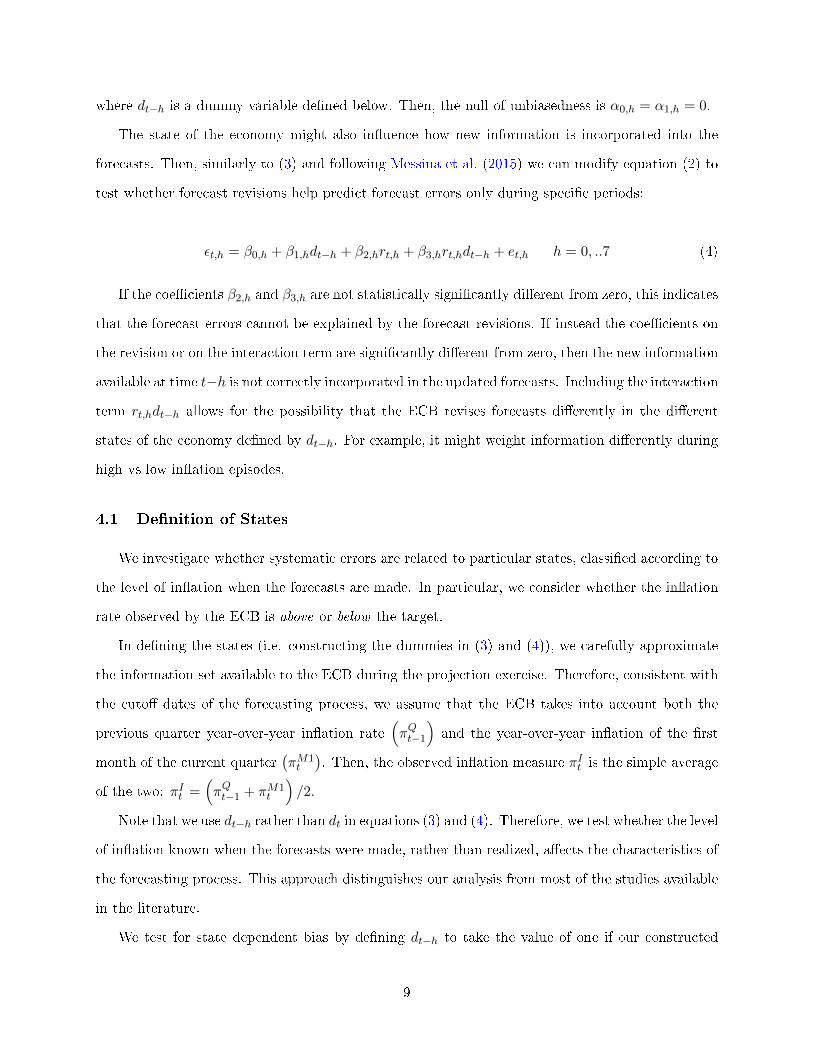
where dt−h is a dummy variable de�ned below. Then, the null of unbiasedness is α0,h = α1,h = 0.
The state of the economy might also in�uence how new information is incorporated into the
forecasts. Then, similarly to (3) and following Messina et al. (2015) we can modify equation (2) to
test whether forecast revisions help predict forecast errors only during speci�c periods:
εt,h = β0,h + β1,hdt−h + β2,hrt,h + β3,hrt,hdt−h + et,h h = 0, ..7 (4)
If the coe�cients β2,h and β3,h are not statistically signi�cantly di�erent from zero, this indicates
that the forecast errors cannot be explained by the forecast revisions. If instead the coe�cients on
the revision or on the interaction term are signi�cantly di�erent from zero, then the new information
available at time t−h is not correctly incorporated in the updated forecasts. Including the interaction
term rt,hdt−h allows for the possibility that the ECB revises forecasts di�erently in the di�erent
states of the economy de�ned by dt−h. For example, it might weight information di�erently during
high vs low in�ation episodes.
4.1 De�nition of States
We investigate whether systematic errors are related to particular states, classi�ed according to
the level of in�ation when the forecasts are made. In particular, we consider whether the in�ation
rate observed by the ECB is above or below the target.
In de�ning the states (i.e. constructing the dummies in (3) and (4)), we carefully approximate
the information set available to the ECB during the projection exercise. Therefore, consistent with
the cuto� dates of the forecasting process, we assume that the ECB takes into account both the
previous quarter year-over-year in�ation rate(πQt−1
)and the year-over-year in�ation of the �rst
month of the current quarter(πM1t
). Then, the observed in�ation measure πIt is the simple average
of the two: πIt =(πQt−1 + πM1
t
)/2.
Note that we use dt−h rather than dt in equations (3) and (4). Therefore, we test whether the level
of in�ation known when the forecasts were made, rather than realized, a�ects the characteristics of
the forecasting process. This approach distinguishes our analysis from most of the studies available
in the literature.
We test for state dependent bias by de�ning dt−h to take the value of one if our constructed
9

measure of observed in�ation πIt is below the in�ation target π∗ in the quarter when the forecast is
made:
dt−h =
1 if πIt−h < π∗
0 otherwise
The ECB price stability de�nition is ambiguous with respect to the level of the target. In
2003 the ECB's Governing Council stated that 'in the pursuit of price stability it aims to maintain
in�ation rates below, but close to, 2% over the medium term'. Following Hartmann and Smets
(2018) we choose 1.8% as the threshold value for the de�nition of the dummy variable dt−h.9 This
results in 45% of observations taking the value of one, indicated as shaded areas in Figure (1). While
most episodes occur during the latest portion of the sample (after 2013Q2), in�ation has dropped
below the target also after the �nancial crisis (2009Q1-2010Q3) and in a few instances in the earlier
portion of the sample.
4.2 Results
Panel B of Table (1) shows the results for bias (equation 3). The coe�cients for the constant
up to h = 5 and for the dummy from h = 2 to h = 4 are highly signi�cant. When the dummy takes
the value of one (zero), the �tted values from the regression are negative (positive), which indicates
that the forecast is higher (lower) than the realized value. This means that when in�ation is below
(above) 1.8%, the ECB tends to overpredict (underpredict) in�ation.10 Interestingly, the size of this
bias, measured as the sum of the coe�cients α0 and α1, increases with the forecast horizon up to
h = 4, and it declines till h = 8. The bias is not only statistically but also economically signi�cant:
when in�ation is above the target, it ranges from 0.09p.p. for one quarter ahead to 0.37p.p. for
four quarters ahead. Overall, we document that the forecasts are biased towards the target at short
and intermediate forecast horizons, between two and four quarters ahead. Note that the bias is
asymmetric in its magnitude: it is larger in absolute value when in�ation is above target than when
9Hartmann and Smets (2018) estimate the reaction functions of the ECB's Governing Council using the samedataset. They conclude that the ECB in�ation aim is 1.8%. This number is in line with estimates by Paloviita et al.(2021) and Rostagno et al. (2019) based on the same data and alternative approaches.
10As mentioned in the Introduction, some papers de�ne state dependence based on the phases of the businesscycle, i.e. recessions or expansions. For completeness, we repeat our analysis according to this classi�cation. Then,the dummy takes the value of one when output growth is below the 25th quantile of its distribution. As shown inTable (7) and (11) of the Appendix, in this case we �nd no state dependent bias nor ine�ciency.
10

below (e.g. �vefold for h = 3).
The literature has suggested several explanations for systematic bias in central banks' forecasts.
Capistran (2008) shows that if a central bank considers in�ation above the target more (less) costly
than in�ation below the target, then it should systematically over(under)-predict in�ation. In his
model the parameter that determines the level of asymmetry in the loss function is constant. This
explanation is di�cult to reconcile with our �ndings because it does not allow for the bias to be
state dependent.11 Romer and Romer (2008) �nd that Greenbook forecasts are of higher quality
than FOMC projections. The di�erence in accuracy can be explained by distinct objectives of
these two sets of forecasts or by di�erent loss functions of the FOMC members and the Fed's sta�
(Ellison and Sargent, 2012). The Greenbook forecasts are con�dential sta� forecasts which aim
at being as accurate as possible, while the FOMC forecasts, which are available in real time, are
used for communication purposes. The ECB produces only one set of forecasts, which serve as
inputs for the Governing Council decisions and are released immediately. Therefore, if there is a
strategic component in published in�ation projections, there might be a tension between accuracy of
forecasts and management of expectations, resulting in a systematic bias. Strategic communication
motives are put forward as an explanation for bias also by Gomez-Barrero and Parra-Polania (2014),
which argue that a central bank might use its published in�ation projections to steer in�ation
expectations of private agents. In their stylized model the incentive to manage expectations is
higher at intermediate horizons, because in the medium term the central bank has both relevant
private information about future shocks hitting the economy and the possibility to a�ect future
in�ation through its in�uence on private agents' expectations. In a laboratory experiment, Du�y
and Heinemann (2021) provide support to this theory and �nd that test subject central bankers
make announcements that deviate from the "true" forecasts in order to manage agents' in�ation
expectations.
While we do not identify the speci�c reason for the systematic, state-dependent bias in the ECB
projections, we believe it might be consistent with the management of in�ation expectations. Also,
the bias is present up to �ve quarters ahead, consistent with the medium-term orientation of the
ECB policy making and the lags in the transmission mechanism of monetary policy.
11To be consistent with our results the model should be modi�ed to allow for a state dependent asymmetryparameter in the loss function of the central bank. Moreover, the size of the asymmetry parameter should di�eracross the two states, to re�ect our �nding that the magnitude of the bias is larger when in�ation is above the target.
11

Panel B of Table (2) shows the estimation results for the e�ciency regression in (4). Similarly
to the bias results, the constant is signi�cant for all (but one) forecasting horizons up to h = 5.
The dummy is also signi�cant at intermediate horizons and retains the negative sign observed in
Table (1). Moreover, for h = 3 we �nd evidence that the forecast revisions do predict the forecast
errors. In particular, when in�ation is above the target, the forecasts are not revised "enough"
as the estimated coe�cient for the revisions is positive. Although not signi�cant, the coe�cient
associated with the interaction term between the dummy and the revisions is negative at h = 3.
However, the sum of β2,3 and β3,3 is still positive but smaller than β2,3. Then, the ECB adjusts its
forecasts less in response to new information when in�ation is above target.12
The underutilization of information documented in Panel B of Table (2) has been interpreted as
evidence of smoothing or information rigidities. Central banks might be cautious about changing
their projections, because such changes convey a message about future economic conditions. Al-
ternatively, policymakers might be concerned for their reputation as forecasters and might prefer
to avoid large and frequent revisions (Scotese (1994), Tillman (2011)). The coe�cient associated
with the revision is signi�cant only in the state dependent regression, and the conservatism of the
ECB projections is stronger when in�ation is above the target. Therefore, when in�ation is high,
and possibly the economic environment is more volatile, the sta� may only partially revise its pre-
vious forecast in order to avoid having to reverse the changes incorporated into the new forecast,
if subsequent data reverse the earlier movements. As a second explanation, our �ndings can also
be interpreted as a rejection of the FIRE hypothesis in favor of models of information rigidities.
According to the noisy-information model, which we believe provides a better description of the
ECB context than the sticky information model, and given the estimates of the parameters β2,3
and β3,3, the relative weight put on new information is 0.64 when in�ation is above target and 0.77
when in�ation is below target. This again re�ects higher conservatism when in�ation is high. Note
that our results do not hold on average, but they are state dependent. Then, models that deviate
from FIRE might need to accommodate an endogenous degree of information rigidities to replicate
12We check the robustness of our results for di�erent values of the target. Results are stronger if we assume a lowertarget (π∗ = 1.7), while the coe�cients retain their sign but lose signi�cance if we assume a higher target, (π∗ = 1.9),see Table (5) and (9) of the Appendix. We further repeat our analysis using alternative assumptions regarding theinformation set available to the ECB at the time of forecasting. As shown in Table (6) and (10) of the Appendix,results are qualitatively unchanged if we assume the in�ation rate observed by the ECB is the nowcast or actualin�ation. Finally, we con�rm that state dependent bias and ine�ciency hold in the published yearly projections, seeTable (8) and (12) in the Appendix.
12
this �nding.
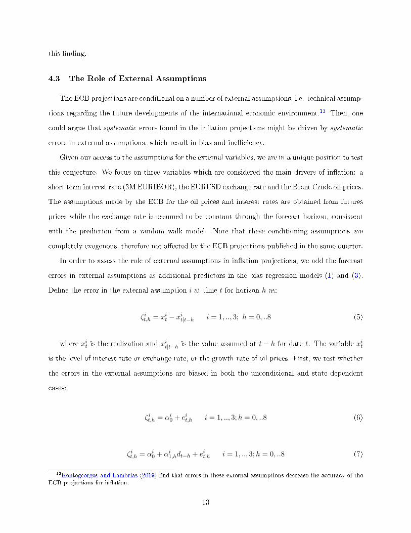
4.3 The Role of External Assumptions
The ECB projections are conditional on a number of external assumptions, i.e. technical assump-
tions regarding the future developments of the international economic environment.13 Then, one
could argue that systematic errors found in the in�ation projections might be driven by systematic
errors in external assumptions, which result in bias and ine�ciency.
Given our access to the assumptions for the external variables, we are in a unique position to test
this conjecture. We focus on three variables which are considered the main drivers of in�ation: a
short term interest rate (3M EURIBOR), the EURUSD exchange rate and the Brent Crude oil prices.
The assumptions made by the ECB for the oil prices and interest rates are obtained from futures
prices while the exchange rate is assumed to be constant through the forecast horizon, consistent
with the prediction from a random walk model. Note that these conditioning assumptions are
completely exogenous, therefore not a�ected by the ECB projections published in the same quarter.
In order to assess the role of external assumptions in in�ation projections, we add the forecast
errors in external assumptions as additional predictors in the bias regression models (1) and (3).
De�ne the error in the external assumption i at time t for horizon h as:
ζit,h = xit − xit|t−h i = 1, .., 3; h = 0, ..8 (5)
where xit is the realization and xit|t−h is the value assumed at t − h for date t. The variable xit
is the level of interest rate or exchange rate, or the growth rate of oil prices. First, we test whether
the errors in the external assumptions are biased in both the unconditional and state dependent
cases:
ζit,h = αi0 + eit,h i = 1, .., 3;h = 0, ..8 (6)
ζit,h = αi0 + αi
1,hdt−h + eit,h i = 1, .., 3;h = 0, ..8 (7)
13Kontogeorgos and Lambrias (2019) �nd that errors in these external assumptions decrease the accuracy of theECB projections for in�ation.
13

where dt−h is the dummy constructed as in 4.1. If we were to �nd some systematic bias in the
conditional model, one could argue that it explains the systematic bias observed in the in�ation
forecast errors. Then, we run the following regression, which includes the error ζit,h as an additional
predictor:
εt,h = βi0,h + βi1,hdt−h + βi2,hζit,h + uit,h i = 1, .., 3; h = 0, ..8 (8)
where, εt,h is the forecast error for predicting in�ation at forecast origin t for horizon h. If the
estimated parameters βi0,h and βi1,h were not signi�cant in (8), while βi2,h were signi�cant, the bias
in the in�ation forecasts could be attributed to the bias in the external assumptions.
Ideally, to carry out our investigation, we would �rst construct a counterfactual series of adjusted
errors for in�ation by using internal ECB models conditioned on the true realization of the external
variables, and then check whether the adjusted errors are biased. However, we are unable to
construct such counterfactual series based on the forecasting models used in real time or to include
the ECB expert judgement. We think that our simple approach is sensible because if systematic
errors in the external assumptions were driving the forecast errors, then the dummy should not have
additional explanatory power.
Results for regressions (6) and (7) are displayed in Table (4) of the Appendix. Panel A shows
that intercept term in the regressions for the short term rate is negative, meaning that on average
the short term rate is assumed to be larger than the realized value. This holds at every horizon,
although the coe�cients are signi�cant only at longer horizons. In the state dependent regressions
the constant is still negative and signi�cant, while the dummy is positive but not statistically
signi�cantly di�erent from zero, suggesting that there is systematic bias only when in�ation is
above target. The bias is large in absolute terms, up to 70 basis points, when in�ation is above
target.
The results for the exchange rate show no evidence of bias on average (Panel B). However,
when in�ation is above (below) the target the exchange rate versus the US dollar is assumed to be
weaker (stronger) than realized. The coe�cients associated with the constant and the dummy are
signi�cant for all horizons higher than two and the bias increases with the horizon.
Finally, the oil price assumptions are not biased on average. In contrast, the state dependent
analysis shows that at very short horizons there is evidence of underprediction (overprediction) when
14

in�ation is higher (lower) than the target. This is consistent with the systematic bias observed for
in�ation. However, the size of the bias is small, amounting to 0.06p.p. at most.
Results for regressions (8) are reported in Panel C1 through C3 of Table (1). Regardless of the
external assumption considered, adding the forecast errors to the bias regression does not alter the
sign, the magnitude nor the signi�cance of the coe�cients observed in Panel B of Table (1). The
interest rate forecast errors are signi�cant only at horizons one and two and enter positively, so that
a larger forecast error for interest rates predicts a larger forecast error for in�ation. Similarly, in
the bias regression augmented by the exchange rate forecast errors, these errors are not signi�cant.
Finally, the oil price forecast errors are highly signi�cant at short term horizons and exhibit a positive
coe�cient, implying that a higher forecast error for oil prices translates into a higher forecast error
for in�ation. While the magnitude of the coe�cient is again unchanged, the constant and the
dummy are signi�cant only for three quarters ahead forecasts.
In sum, we �nd evidence of systematic over(under)prediction for medium term projections when
in�ation is lower (higher) than the target even when controlling for the errors in external assump-
tions.
5 Conclusion
Using a con�dential dataset of ECB macroeconomic quarterly projections we document three
novel �ndings that relate the bias and e�ciency of the ECB in�ation forecasts to the level of in�ation
at the time of forecasting: (i) a systematic bias towards the target at medium horizons, which implies
over (under) prediction when in�ation is low (high); (ii) a larger bias when in�ation is above the
target; (iii) ine�ciency, resulting in underutilization of new information at medium horizons when
in�ation is above target.
Our results suggest that looking at state dependence is crucial. We argue that theoretical
models are unable to replicate the observed state dependence in bias and e�ciency and hence, they
might need to be reformulated in order to match these features of the forecasts. Given the lack
of theoretical models that can simultaneously account for state dependent bias and ine�ciency in
central banks' forecasts, this paper has the potential to start a line of theoretical research that
rationalizes these �ndings.
15

Our investigation of the properties of the published projections is relevant also from a policy
perspective, in particular for the ongoing ECB strategy review: the forecasts form the basis for the
monetary policy decisions of the ECB Governing Council and represent an important communication
tool. While the reasons behind our �ndings are beyond the scope of this paper, we conjecture
that the evidence of state dependent bias and ine�ciency might be related to strategic motives
in monetary policy communication. These are particularly strong at the intermediate horizons,
re�ecting the medium-term orientation of monetary policy making.
16
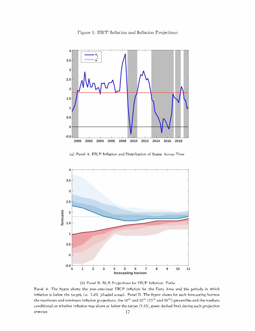
Figure 1: HICP In�ation and In�ation Projections
2000 2002 2004 2006 2008 2010 2012 2014 2016 2018-0.5
0
0.5
1
1.5
2
2.5
3
3.5
4t*
(a) Panel A: HICP In�ation and Distribution of States Across Time
0 1 2 3 4 5 6 7 8 9 10 11forecasting horizon
-0.5
0
0.5
1
1.5
2
2.5
3
3.5
4
fore
cast
s
(b) Panel B: ECB Projections for HICP In�ation: Paths
Panel A. The �gure shows the year-over-year HICP in�ation for the Euro Area and the periods in which
in�ation is below the target, i.e. 1.8% (shaded areas). Panel B. The �gure shows for each forecasting horizon
the maximum and minimum in�ation projections, the 10th and 25th (75th and 90th) percentiles and the medians
conditional on whether in�ation was above or below the target (1.8%, green dashed line) during each projection
exercise. 17

Table 1: Bias in ECB In�ation Forecasts
Forecast Horizonh = 0 1 2 3 4 5 6 7 8
Panel A: Overall Sample
c -0.02 0.03 0.07 0.11 0.13 0.14 0.11 0.07 0.02(0.01) (0.04) (0.08) (0.11) (0.14) (0.15) (0.15) (0.16) (0.16)
Panel B: Asymmetry
c -0.03* 0.09* 0.19** 0.32*** 0.37** 0.35* 0.31 0.22 0.14(0.02) (0.05) (0.09) (0.13) (0.16) (0.18) (0.19) (0.20) (0.20)
dt 0.03 -0.11 -0.25* -0.38* -0.44* -0.38 -0.34 -0.25 -0.16(0.03) (0.08) (0.15) (0.20) (0.27) (0.29) (0.30) (0.32) (0.33)
Panel C1: Short Term Interest Rate
c -0.03* 0.11** 0.23** 0.37*** 0.44** 0.46** 0.42** 0.33 0.26(0.02) (0.05) (0.09) (0.13) (0.17) (0.19) (0.20) (0.21) (0.22)
ζt -0.12 0.36** 0.37** 0.27 0.24 0.25 0.21 0.17 0.17(0.20) (0.13) (0.14) (0.13) (0.12) (0.09) (0.08) (0.07) (0.07)
dt 0.03 -0.14* -0.28** -0.41** -0.48* -0.44 -0.39 -0.28 -0.18(0.03) (0.08) (0.14) (0.20) (0.26) (0.28) (0.30) (0.31) (0.32)
Panel C2: Exchange Rate
c -0.03 0.10** 0.19** 0.32** 0.34** 0.26 0.15 0.02 -0.10(0.02) (0.05) (0.09) (0.13) (0.17) (0.19) (0.19) (0.19) (0.18)
ζt -0.72 -0.94 0.16 0.11 0.65 1.62 2.49 2.93 3.18(1.00) (0.73) (0.88) (1.04) (1.17) (1.21) (1.16) (1.03) (0.93)
dt 0.03 -0.13* -0.24 -0.37* -0.38 -0.21 -0.03 0.14 0.28(0.03) (0.08) (0.15) (0.22) (0.28) (0.31) (0.31) (0.30) (0.30)
Panel C3: Oil Prices
c -0.02 0.02 0.12 0.25** 0.29* 0.30* 0.27 0.19 0.10(0.02) (0.04) (0.09) (0.13) (0.17) (0.17) (0.18) (0.18) (0.18)
ζt 0.78*** 1.66*** 1.24*** 1.18* 1.39 1.19 1.01 1.41 1.51(0.30) (0.26) (0.45) (0.64) (0.85) (0.84) (0.86) (0.91) (0.93)
dt 0.01 -0.05 -0.18 -0.35* -0.41 -0.40 -0.37 -0.25 -0.15(0.03) (0.07) (0.14) (0.20) (0.26) (0.26) (0.28) (0.29) (0.29)
Note: Estimated coe�cients from regressions (1), (3) and (8). Newey-West standard errors are in parenthe-sis. Stars denote the 10% (*), 5% (**) and 1% (***) signi�cance level. For regressions involving the shortterm interest rates, note that before 2006 an assumption of constant short term interest rates was used.
18
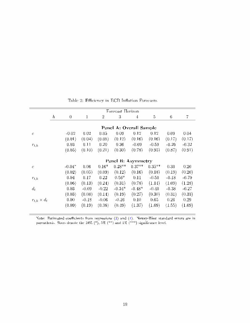
Table 2: E�ciency in ECB In�ation Forecasts
Forecast Horizonh = 0 1 2 3 4 5 6 7
Panel A: Overall Sample
c -0.02 0.02 0.05 0.09 0.12 0.12 0.09 0.04(0.01) (0.04) (0.08) (0.12) (0.16) (0.16) (0.17) (0.17)
rt,h 0.03 0.11 0.20 0.36 -0.09 -0.59 -0.26 -0.32(0.05) (0.10) (0.21) (0.30) (0.78) (0.95) (0.87) (0.91)
Panel B: Asymmetry
c -0.04* 0.06 0.16* 0.28** 0.37** 0.35** 0.30 0.20(0.02) (0.05) (0.09) (0.12) (0.16) (0.18) (0.19) (0.20)
rt,h 0.04 0.17 0.22 0.56* 0.11 -0.50 -0.18 -0.70(0.06) (0.13) (0.24) (0.31) (0.78) (1.14) (1.09) (1.28)
dt 0.03 -0.09 -0.22 -0.34* -0.48* -0.40 -0.38 -0.27(0.03) (0.08) (0.14) (0.19) (0.27) (0.30) (0.31) (0.33)
rt,h × dt 0.00 -0.18 -0.06 -0.26 0.10 0.65 0.26 0.29(0.09) (0.19) (0.36) (0.49) (1.37) (1.69) (1.55) (1.69)
Note: Estimated coe�cients from regressions (2) and (4). Newey-West standard errors are inparenthesis. Stars denote the 10% (*), 5% (**) and 1% (***) signi�cance level.
19
References
Alessi, L., E. Ghysel, L. Onorante, R. Peach, and S. Potter (2014). Central Bank Macroeconomic
Forecasting During the Global Financial Crisis: The European Central Bank and Federal Reserve
Bank of New York Experiences. Journal of Business and Economic Statistics 32 (4), 483�500.
Angeletos, G.-M., Z. Huo, and K. A. Sastry (2020). Imperfect Macroeconomic Expectations: Evi-
dence and Theory. NBER Working Papers 27308, National Bureau of Economic Research, Inc.
Arai, N. (2016). Evaluating the e�ciency of the fomc's new economic projections. Journal of Money,
Credit and Banking 48 (5), 1019�1039.
Bordalo, P., N. Gennaioli, Y. Ma, and A. Shleifer (2020). Overreaction in macroeconomic expecta-
tions. American Economic Review 110 (9), 2748�2782.
Capistran, C. (2008). Bias in Federal Reserve In�ation Forecasts: Is the Federal Reserve Irrational
of Just Cautious? Journal of Monetary Economics 55, 1415�1427.
Charemza, W. and D. Ladley (2016). Central banks' forecasts and their bias: Evidence, e�ects and
explanation. International Journal of Forecasting 32, 804�817.
Clements, M. P., F. Joutz, and H. O. Stekler (2007). An evaluation of the forecasts of the federal
reserve: a pooled approach. Journal of Applied Econometrics 22, 121�136.
Coibion, O. and Y. Gorodnichenko (2015). Information rigidity and the expectations formation
process: A simple framework and new facts. American Economic Review 105 (8), 2644�2678.
Coibion, O., Y. Gorodnichenko, S. Kumar, and M. Pedemonte (2020). In�ation expectations as a
policy tool? Journal of International Economics 124, 2�26.
Du�y, J. and F. Heinemann (2021). Central bank reputation, cheap talk and transparency as
substitutes for commitment: Experimental evidence. Journal of Monetary Economics 117, 887�
903.
El-Shagi, M., S. Giesen, and A. Jung (2016). Revisiting the relative forecast performances of fed sta�
and private forecasters: A dynamic approach. International Journal of Forecasting 32, 313�323.
20

Ellison, M. and T. J. Sargent (2012). A defence of the FOMC. International Economic Re-
view 53 (34), 1047�1065.
Fawcett, N., L. Koerber, R. Masolo, and M. Waldron (2015). Evaluating UK Point and Density
Forecasts from an Estimated DSGE Model: the Role of O�-Model Information Over the Financial
Crisis. Working Papers 538, Bank of England.
Fuhrer, J. (2018). Intrinsic Expectations Persistence: Evidence from Professional and Household
Survey Expectations. Working Paper 2018-09, Federal Reserve Bank of Boston.
Fujiwara, I. (2005). Is the central bank's publication of economic forecasts in�uential? Economics
Letters 89, 255�261.
Gomez-Barrero, S. and J. A. Parra-Polania (2014). Central bank strategic forecasting. Contemporary
Economic Policy 32 (4), 802�810.
Hartmann, P. and F. Smets (2018). The First Twenty Years of the European Central Bank: Mon-
etary Policy. Working Papers 2219, European Central Bank.
Herbert, S. (2020). State-Dependent Central Bank Communication with Heterogeneous Beliefs.
mimeo.
Holden, K. and D. A. Peel (1990). On testing for unbiasedness and e�ciency of forecasts. The
Manchester School 58 (2), 120�127.
Hubert, P. (2014). Fomc forecasts as a focal point for private expectations. Journal of Money,
Credit and Banking 46 (7), 1381�1420.
Hubert, P. (2015). Do central bank forecasts in�uence private agents? forecasting performance
versus signals. Journal of Money, Credit and Banking 47 (4), 771�789.
Hubert, P. (2017). Qualitative and quantitative central bank communication and in�ation expec-
tations. B.E. Journal of Macroeconomics 17 (1), 1�41.
Iversen, J., S. Laséen, S. L. H., and U. Söderström (2016). Real-Time Forecasting for Monetary
Policy Analysis: the Case of Sveriges Riksbank. Working Papers 318, Sveriges Riksbank.
21

Kohlhas, A. N. and A. Walther (2021). Asymmetric attention. American Economic Review forth-
coming.
Kontogeorgos, G. and K. Lambrias (2019). An Analysis of the Eurosystem/ECB Projections. Work-
ing Papers 2291, European Central Bank.
Lahiri, K. and X. Sheng (2008). Evolution of forecast disagreement in a bayesian learning model.
Journal of Econometrics 144, 325�340.
Loungani, P., H. Stekler, and N. Tamirisa (2013). Information rigidity in growth forecasts: Some
cross-country evidence. International Journal of Forecasting 29, 605�621.
Lyziak, T. and M. Paloviita (2018). On the formation of in�ation expectations in turbulent times:
The case of the euro area. Economic Modelling 72, 132�139.
Messina, J., T. M. Sinclair, and H. Stekler (2015). What can we learn from revisions to the greenbook
forecasts? Journal of Macroeconomics 45, 54�62.
Mincer, J. and V. Zarnowitz (1969, June). The Evaluation of Economic Forecasts, pp. 3�46. Eco-
nomic Forecasts and Expectations: Analysis of Forecasting Behavior and Performance. NBER
Books.
Nordhaus, W. (1987). Forecasting e�ciency, concepts, and applications. Review of Economic and
Statistics 69, 667�674.
Paloviita, M., M. Haavio, P. Jalasjoki, and J. Kilponen (2021). What does "below, but close to, two
per cent" mean? assessing the ecb's reaction function with real time data. International Journal
of Central Banking , forthcoming.
Potter, S. (2011). The Failure to Forecast the Great Recession. Technical report,
https://libertystreeteconomics.newyorkfed.org/.
Romer, C. D. and D. H. Romer (2008). The fomc versus the sta�: Where can monetary policymakers
add value? American Economic Review 98 (2).
22

Rostagno, M., C. Altavilla, G. Carboni, W. Lemke, R. Motto, A. S. Guilhem, and J. Yiangou
(2019). A Tale of Two Decades: The ECB's Monetary Policy at 20. WP N. 2346, European
Central Bank.
Scotese, C. A. (1994). Forecast smoothing and the optimal under-utilization of information at the
federal reserve. Journal of Macroeconomics 16 (4), 653�670.
Sinclair, T. M., F. Joutz, and H. Stekler (2010). Can the fed predict the state of the economy?
Economic Letters 108, 28�32.
Stockton, D. (2012). Review of the Monetary Policy Committee's Forecasting Capability. Technical
report, Report Presented to the Court of the Bank of England.
Tillman, P. (2011). Reputation and Forecast Revisions: Evidence from the FOMC. Working paper
201128, MAGKS Papers on Economics.
23
Appendix
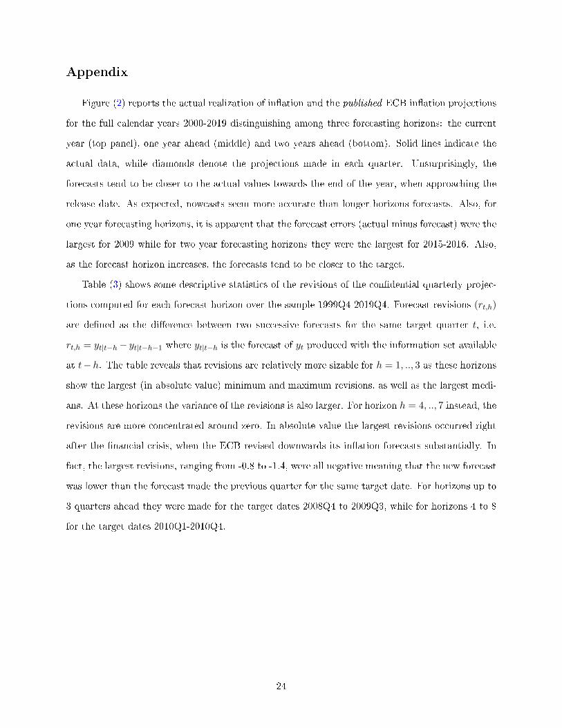
Figure (2) reports the actual realization of in�ation and the published ECB in�ation projections
for the full calendar years 2000-2019 distinguishing among three forecasting horizons: the current
year (top panel), one year ahead (middle) and two years ahead (bottom). Solid lines indicate the
actual data, while diamonds denote the projections made in each quarter. Unsurprisingly, the
forecasts tend to be closer to the actual values towards the end of the year, when approaching the
release date. As expected, nowcasts seem more accurate than longer horizons forecasts. Also, for
one year forecasting horizons, it is apparent that the forecast errors (actual minus forecast) were the
largest for 2009 while for two year forecasting horizons they were the largest for 2015-2016. Also,
as the forecast horizon increases, the forecasts tend to be closer to the target.
Table (3) shows some descriptive statistics of the revisions of the con�dential quarterly projec-
tions computed for each forecast horizon over the sample 1999Q4-2019Q4. Forecast revisions (rt,h)
are de�ned as the di�erence between two successive forecasts for the same target quarter t, i.e.
rt,h = yt|t−h − yt|t−h−1 where yt|t−h is the forecast of yt produced with the information set available
at t−h. The table reveals that revisions are relatively more sizable for h = 1, .., 3 as these horizons
show the largest (in absolute value) minimum and maximum revisions, as well as the largest medi-
ans. At these horizons the variance of the revisions is also larger. For horizon h = 4, .., 7 instead, the
revisions are more concentrated around zero. In absolute value the largest revisions occurred right
after the �nancial crisis, when the ECB revised downwards its in�ation forecasts substantially. In
fact, the largest revisions, ranging from -0.8 to -1.4, were all negative meaning that the new forecast
was lower than the forecast made the previous quarter for the same target date. For horizons up to
3 quarters ahead they were made for the target dates 2008Q4 to 2009Q3, while for horizons 4 to 8
for the target dates 2010Q1-2010Q4.
24
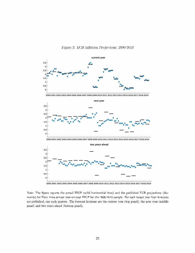
Figure 2: ECB In�ation Projections: 2000-2019
2000 2001 2002 2003 2004 2005 2006 2007 2008 2009 2010 2011 2012 2013 2014 2015 2016 2017 2018 2019
0
0.5
1
1.5
2
2.5
3
3.5
current year
2000 2001 2002 2003 2004 2005 2006 2007 2008 2009 2010 2011 2012 2013 2014 2015 2016 2017 2018 2019
0
0.5
1
1.5
2
2.5
3
3.5
next year
2000 2001 2002 2003 2004 2005 2006 2007 2008 2009 2010 2011 2012 2013 2014 2015 2016 2017 2018 2019
0
0.5
1
1.5
2
2.5
3
3.5
two years ahead
Note: The �gure reports the actual HICP (solid horizonthal lines) and the published ECB projections (dia-
monds) for Euro Area annual year-on-year HICP for the 2000-2019 sample. For each target year four forecasts
are published, one each quarter. The forecast horizons are the current year (top panel), the next year (middle
panel) and two years ahead (bottom panel).
25
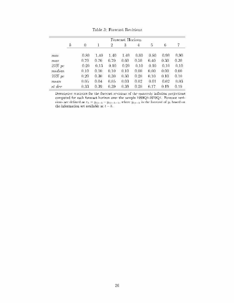
Table 3: Forecast Revisions
Forecast Horizonh = 0 1 2 3 4 5 6 7
min -0.80 -1.40 -1.40 -1.40 -0.60 -0.80 -0.90 -0.90max 0.70 0.70 0.70 0.60 0.50 0.40 0.30 0.3025% pc -0.20 -0.13 -0.10 -0.20 -0.10 -0.10 -0.10 -0.10median 0.10 0.10 0.10 0.10 0.00 0.00 0.00 0.0075% pc 0.20 0.30 0.30 0.30 0.20 0.10 0.10 0.10mean 0.05 0.04 0.05 0.03 0.02 -0.01 -0.02 -0.03st dev 0.33 0.39 0.39 0.39 0.20 0.17 0.19 0.19
Descriptive statistics for the forecast revisions of the quarterly in�ation projectionscomputed for each forecast horizon over the sample 1999Q4-2019Q4. Forecast revi-sions are de�ned as rh = yt|t−h − yt|t−h−1, where yt|t−h is the forecast of yt based onthe information set available at t− h.
26
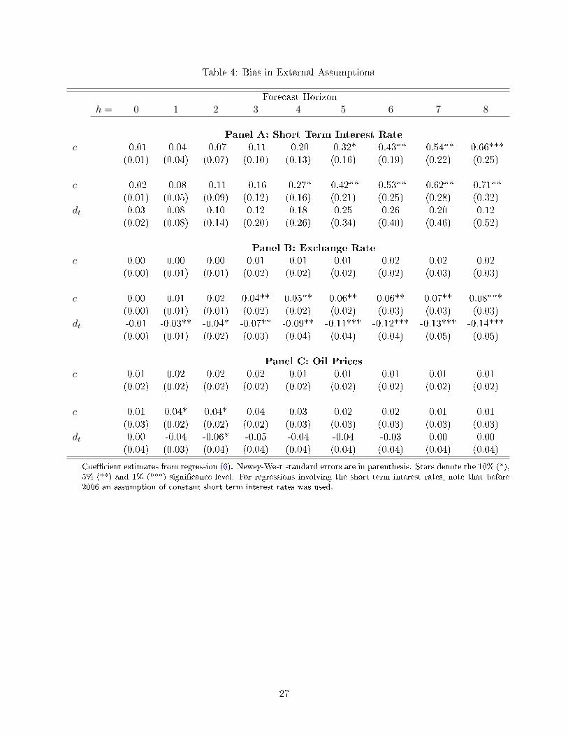
Table 4: Bias in External Assumptions
Forecast Horizonh = 0 1 2 3 4 5 6 7 8
Panel A: Short Term Interest Rate
c -0.01 -0.04 -0.07 -0.11 -0.20 -0.32* -0.43** -0.54** -0.66***(0.01) (0.04) (0.07) (0.10) (0.13) (0.16) (0.19) (0.22) (0.25)
c -0.02 -0.08 -0.11 -0.16 -0.27* -0.42** -0.53** -0.62** -0.71**(0.01) (0.05) (0.09) (0.12) (0.16) (0.21) (0.25) (0.28) (0.32)
dt 0.03 0.08 0.10 0.12 0.18 0.25 0.26 0.20 0.12(0.02) (0.08) (0.14) (0.20) (0.26) (0.34) (0.40) (0.46) (0.52)
Panel B: Exchange Rate
c 0.00 0.00 0.00 0.01 0.01 0.01 0.02 0.02 0.02(0.00) (0.01) (0.01) (0.02) (0.02) (0.02) (0.02) (0.03) (0.03)
c 0.00 0.01 0.02 0.04** 0.05** 0.06** 0.06** 0.07** 0.08***(0.00) (0.01) (0.01) (0.02) (0.02) (0.02) (0.03) (0.03) (0.03)
dt -0.01 -0.03** -0.04* -0.07** -0.09** -0.11*** -0.12*** -0.13*** -0.14***(0.00) (0.01) (0.02) (0.03) (0.04) (0.04) (0.04) (0.05) (0.05)
Panel C: Oil Prices
c 0.01 0.02 0.02 0.02 0.01 0.01 0.01 0.01 0.01(0.02) (0.02) (0.02) (0.02) (0.02) (0.02) (0.02) (0.02) (0.02)
c 0.01 0.04* 0.04* 0.04 0.03 0.02 0.02 0.01 0.01(0.03) (0.02) (0.02) (0.02) (0.03) (0.03) (0.03) (0.03) (0.03)
dt 0.00 -0.04 -0.06* -0.05 -0.04 -0.04 -0.03 0.00 0.00(0.04) (0.03) (0.04) (0.04) (0.04) (0.04) (0.04) (0.04) (0.04)
Coe�cient estimates from regression (6). Newey-West standard errors are in parenthesis. Stars denote the 10% (*),5% (**) and 1% (***) signi�cance level. For regressions involving the short term interest rates, note that before2006 an assumption of constant short term interest rates was used.
27
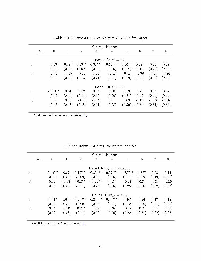
Table 5: Robustness for Bias: Alternative Values for Target
Forecast Horizonh = 0 1 2 3 4 5 6 7 8
Panel A: π∗ = 1.7c -0.03* 0.08* 0.19** 0.31*** 0.36*** 0.36** 0.32* 0.24 0.17
(0.02) (0.05) (0.09) (0.13) (0.16) (0.18) (0.19) (0.20) (0.20)dt 0.03 -0.10 -0.23 -0.36* -0.43 -0.42 -0.38 -0.31 -0.24
(0.03) (0.08) (0.15) (0.21) (0.27) (0.29) (0.31) (0.32) (0.33)
Panel B: π∗ = 1.9c -0.04** 0.04 0.12 0.24 0.20 0.18 0.21 0.14 0.12
(0.02) (0.06) (0.11) (0.15) (0.20) (0.21) (0.22) (0.22) (0.22)dt 0.05 0.00 -0.04 -0.12 0.01 0.03 -0.07 -0.03 -0.08
(0.03) (0.08) (0.15) (0.21) (0.28) (0.30) (0.31) (0.31) (0.32)
Coe�cient estimates from regression (3).
Table 6: Robustness for Bias: Information Set
Forecast Horizonh = 0 1 2 3 4 5 6 7 8
Panel A: πIt−h = πt−h|t−hc -0.04** 0.07 0.19*** 0.33*** 0.37*** 0.38*** 0.32* 0.23 0.14
(0.02) (0.05) (0.09) (0.12) (0.16) (0.17) (0.19) (0.19) (0.20)dt 0.04 -0.08 -0.25* -0.41** -0.45* -0.47 -0.39 -0.28 -0.16
(0.03) (0.08) (0.14) (0.20) (0.26) (0.28) (0.30) (0.32) (0.33)
Panel B: πIt−h = πt−hc -0.04* 0.09* 0.20*** 0.33*** 0.36*** 0.34* 0.26 0.17 0.13
(0.02) (0.05) (0.09) (0.13) (0.17) (0.19) (0.20) (0.21) (0.21)dt 0.04 -0.10 -0.24* -0.38* -0.39 -0.32 -0.22 -0.11 -0.11
(0.03) (0.08) (0.14) (0.20) (0.26) (0.29) (0.31) (0.32) (0.33)
Coe�cient estimates from regression (3).
28

Table 7: Robustness for Bias: Technical Recessions
Forecast Horizonh = 0 1 2 3 4 5 6 7 8
Panel A: Overall Sample
c -0.02 0.03 0.07 0.11 0.13 0.14 0.11 0.07 0.02(0.01) (0.04) (0.08) (0.11) (0.14) (0.15) (0.15) (0.16) (0.16)
Panel B: Asymmetry
c -0.02 0.07 0.14 0.25** 0.29* 0.32* 0.27 0.21 0.14(0.02) (0.05) (0.09) (0.12) (0.16) (0.17) (0.18) (0.18) (0.19)
dt 0.01 -0.11 -0.18 -0.28 -0.34 -0.45 -0.35 -0.30 -0.21(0.03) (0.09) (0.18) (0.24) (0.31) (0.32) (0.34) (0.35) (0.36)
Coe�cient estimates from regression (3). We de�ne the state according to the phases of the businesscycle. Then, the dummy takes the value of one during technical recessions, when output growth isbelow the 25th quantile of its distribution.
Table 8: Bias in Published Projections
Forecast Horizoncurrent year next year year after next
Panel A: Overall Sample
c 0.02 0.14 0.12(0.02) (0.12) (0.15)
Panel B: Asymmetry
c 0.04 0.28** 0.18(0.03) (0.14) (0.19)
dt -0.05 -0.35 -0.17(0.05) (0.23) (0.30)
Coe�cient estimates from regression (3).
29

Table 9: E�ciency of ECB In�ation Forecasts: Alternative Values for Target
Forecast Horizonh = 0 1 2 3 4 5 6 7
Panel A: π∗ = 1.7c -0.04* 0.07 0.16* 0.28*** 0.36** 0.35** 0.30* 0.21
(0.02) (0.05) (0.09) (0.12) (0.16) (0.17) (0.18) (0.20)rt,h 0.04 0.15 0.23 0.56** 0.21 -0.48 -0.33 -0.84
(0.06) (0.11) (0.21) (0.29) (0.71) (0.89) (0.84) (0.95)dt 0.03 -0.10 -0.22 -0.34* -0.47* -0.38 -0.42 -0.29
(0.03) (0.08) (0.14) (0.19) (0.27) (0.29) (0.30) (0.32)rt,h × dt 0.01 -0.17 -0.05 -0.24 0.16 2.54 2.04 1.43
(0.09) (0.20) (0.38) (0.51) (1.59) (2.17) (1.85) (1.79)
Panel B: π∗ = 1.9c -0.06* 0.01 0.06 0.16 0.19 0.19 0.21 0.15
(0.02) (0.06) (0.11) (0.14) (0.20) (0.21) (0.22) (0.22)rt,h 0.10 0.23 0.33 0.72** 0.18 -0.45 -0.16 -1.03
(0.07) (0.14) (0.27) (0.37) (0.90) (1.26) (1.23) (1.41)dt 0.06 0.03 0.02 -0.03 -0.01 0.04 -0.10 -0.08
(0.03) (0.08) (0.15) (0.20) (0.27) (0.30) (0.31) (0.33)rt,h × dt -0.06 -0.18 -0.10 -0.36 0.32 0.85 0.21 0.83
(0.10) (0.20) (0.37) (0.51) (1.39) (1.77) (1.62) (1.77)
Note: Estimated coe�cients from regressions (4). Newey-West standard errors are in parenthesis.Stars denote the 10% (*), 5% (**) and 1% (***) signi�cance level.
30
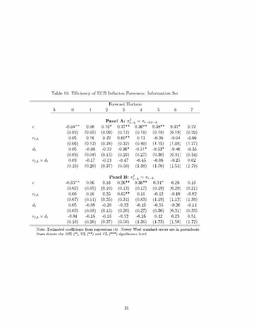
Table 10: E�ciency of ECB In�ation Forecasts: Information Set
Forecast Horizonh = 0 1 2 3 4 5 6 7
Panel A: πIt−h = πt−h|t−hc -0.04** 0.06 0.16* 0.27** 0.36** 0.38** 0.32* 0.22
(0.02) (0.05) (0.09) (0.12) (0.16) (0.18) (0.19) (0.20)rt,h 0.05 0.16 0.22 0.60** 0.13 -0.36 -0.04 -0.66
(0.06) (0.13) (0.24) (0.32) (0.80) (1.15) (1.08) (1.27)dt 0.05 -0.06 -0.22 -0.36* -0.51* -0.53* -0.46 -0.35
(0.03) (0.08) (0.15) (0.20) (0.27) (0.30) (0.31) (0.34)rt,h × dt 0.03 -0.17 -0.13 -0.47 -0.45 -0.06 -0.25 0.02
(0.10) (0.20) (0.37) (0.50) (1.38) (1.70) (1.55) (1.70)
Panel B: πIt−h = πt−hc -0.05** 0.06 0.16 0.26** 0.36** 0.34* 0.26 0.16
(0.02) (0.05) (0.10) (0.13) (0.17) (0.19) (0.20) (0.21)rt,h 0.06 0.16 0.25 0.65** 0.16 -0.42 -0.19 -0.82
(0.07) (0.14) (0.25) (0.34) (0.83) (1.19) (1.12) (1.30)dt 0.05 -0.08 -0.20 -0.32 -0.43 -0.35 -0.26 -0.14
(0.03) (0.08) (0.15) (0.20) (0.27) (0.30) (0.31) (0.33)rt,h × dt -0.01 -0.16 -0.16 -0.52 -0.16 0.42 0.23 0.51
(0.10) (0.20) (0.37) (0.50) (1.36) (1.73) (1.58) (1.72)
Note: Estimated coe�cients from regressions (4). Newey-West standard errors are in parenthesis.Stars denote the 10% (*), 5% (**) and 1% (***) signi�cance level.
31
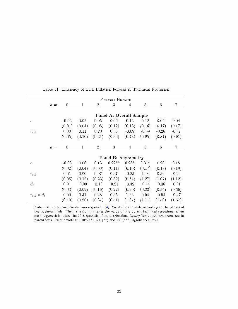
Table 11: E�ciency of ECB In�ation Forecasts: Technical Recession
Forecast Horizonh = 0 1 2 3 4 5 6 7
Panel A: Overall Sample
c -0.02 0.02 0.05 0.09 0.12 0.12 0.09 0.04(0.01) (0.04) (0.08) (0.12) (0.16) (0.16) (0.17) (0.17)
rt,h 0.03 0.11 0.20 0.36 -0.09 -0.59 -0.26 -0.32(0.05) (0.10) (0.21) (0.30) (0.78) (0.95) (0.87) (0.91)
h = 0 1 2 3 4 5 6 7
Panel B: Asymmetry
c -0.03 0.06 0.13 0.22** 0.28* 0.31* 0.26 0.18(0.02) (0.04) (0.08) (0.11) (0.15) (0.17) (0.18) (0.19)
rt,h 0.01 0.00 0.07 0.37 -0.23 -0.04 0.39 -0.29(0.05) (0.12) (0.23) (0.32) (0.84) (1.27) (1.07) (1.12)
dt 0.01 -0.09 -0.13 -0.21 -0.32 -0.44 -0.36 -0.31(0.03) (0.09) (0.16) (0.22) (0.30) (0.32) (0.34) (0.36)
rt,h × dt 0.09 0.31 0.48 0.35 1.33 0.04 -0.95 -0.47(0.10) (0.20) (0.37) (0.51) (1.37) (1.71) (1.56) (1.67)
Note: Estimated coe�cients from regression (4). We de�ne the state according to the phases ofthe business cycle. Then, the dummy takes the value of one during technical recessions, whenoutput growth is below the 25th quantile of its distribution. Newey-West standard errors are inparenthesis. Stars denote the 10% (*), 5% (**) and 1% (***) signi�cance level.
32

Table 12: E�ciency of PublishedProjections
Forecast Horizoncurrent year next year
Panel A: Overall Sample
c 0.02 0.12(0.02) (0.09)
rt,h 0.00 1.39***(0.03) (0.24)
Panel B: Asymmetry
c 0.10*** 0.46***(0.05) (0.09)
rt,h -0.14** 0.30(0.07) (0.28)
dt -0.10 -0.57***(0.06) (0.16)
rt,h × dt 0.17* 1.04***(0.09) (0.45)
Note: Estimated coe�cients from regres-sion (4). Newey-West standard errors are inparenthesis. Stars denote the 10% (*), 5%(**) and 1% (***) signi�cance level.
33
Bank of Finland Research Discussion Papers 2021 ISSN 1456-6184, online
1/2021 Giovanni Caggiano and Efrem Castelnuovo Global Uncertainty ISBN 978-952-323-365-2, online
2/2021 Maija Järvenpää and Aleksi Paavola Investor monitoring, money-likeness and stability of money market funds ISBN 978-952-323-366-9, online
3/2021 Diego Moreno and Tuomas Takalo Precision of Public Information Disclosures, Banks’ Stability and Welfare ISBN 978-952-323-368-3, online
4/2021 Gene Ambrocio Euro Area Business Confidence and Covid-19 ISBN 978-952-323-370-6, online
5/2021 Markus Haavio and Olli-Matti Laine Monetary policy rules and the effective lower bound in the Euro area ISBN 978-952-323-371-3, online
6/2021 Seppo Honkapohja and Nigel McClung On robustness of average inflation targeting ISBN 978-952-323-373-7, online
7/2021 Eleonora Granziera, Pirkka Jalasjoki and Maritta Paloviita The bias and efficiency of the ECB inflation projections: a State dependent analysis ISBN 978-952-323-374-4, online