Bank Integration and Business Volatility

Bank Integration and Business Volatility

Donald Morgan,Bertrand Rime,

Philip E. Strahan*

This draft: November 2001

AbstractWe investigate how bank migration across state lines over the last quarter century hasaffected the size and covariance of business fluctuations within states. Starting with atwo-state version of the unit banking model in Holmstrom and Tirole (1997), weconclude that the theoretical effect of integration on business fluctuations is ambiguousbecause integration dampens the impact of bank capital shocks but amplifies the impactof firm collateral shocks. The net effect empirically seems stabilizing, however, as wefind fluctuations in employment growth within states falls as integration rises, especiallywhen we instrument for the level of integration and control for employment compositionwithin states. Integration also weakens the link between bank capital growth withinstates and growth in state employment and bank lending.

* Morgan: Research Department, Federal Reserve Bank of New York, 33 Liberty Street, NY, NY, 10045;212.720.2000. Rime: Swiss National Bank, Börsenstr. 15, Postfach, 8022 Zürich. Strahan: Carroll Schoolof Management, Boston College, 140 Commonwealth Ave., Chestnut Hill, MA 02467.Email and phone: [email protected]. 212.720.6573; [email protected]; [email protected],617.552.6430, http://www2.bc.edu/~strahan;

The views expressed are those of the authors and do not necessarily reflect the position of the SwissNational Bank, the Federal Reserve Bank of New York, or the Federal Reserve System. We thank JeanTirole for his comments and Paul Edelstein and Shana Wang for their research assistance.

2

2

I. Introduction

The United States once had 50 little banking systems, one per state, because all

the states effectively blocked entry by out-of-state banks. Under that segregated system,

the fate of each state and its banks were closely tied; as went the states, so went the

banks. Farm price deflation in the early 1980s bankrupted many farmers and many farm

banks, just as falling oil prices in the late 80s wiped out a lot of Texans and Texas banks.

Now that states have mostly opened their borders to out-of-state banks, the banking

industry is converging toward a single system dominated by the very large holding

companies with banks operating in many states (Map).

Whether this integration of our banking system has any real, macro consequences

depends on whether these intermediaries provide any unique services to the economy. If

not, if banks are just another thread in an irrelevant financial veil, their integration is

largely irrelevant; we might expect second and third order benefits at most in the form of

paper work reduction and back-office consolidation.

Integration gets a lot more interesting if banks are viewed as essential producers

of important monitoring and risk sharing services. As a starting point for thinking about

those more important effects, our paper lays out a modified version of Holmstrom and

Tirole’s (1997) banking model. Bankers in their model can prevent moral hazard— by

monitoring firms— and they can commit moral hazard— by neglecting to monitor. These

hazards make the equilibrium rate of investment spending in the economy a function of

the level of firm collateral and bank capital; these seemingly backward-looking state

variables give firms and bankers a stake in future investment outcomes, and that stake

3

3

keeps both parties honest. Exogenous shocks to either variable cause equilibrium

investment to fall, i.e., collateral damage and capital crunches are both contractionary.

To see whether interstate banking alters those effects, we add a second (physical)

state to the H-T model. Both collateral and capital shocks are still contractionary, not

surprisingly, but interstate banking changes their magnitudes: bank capital shocks in state

A have a smaller impact with interstate banking, and the impact of collateral shocks gets

bigger. These derivatives are fairly complicated functions of the frictions in the model,

but the intuition is straightforward and general: a holding company that is diversified

across two states can import capital to state A if lending opportunities there are still good,

but a collateral shock in state A will lead the holding company to export capital and

lending away from that state.

Rather than try to identify these effects separately (the econometric equivalent of

laser surgery it seems to us), we ask the data whether the net effect of integration has

been to make state economies more or less stable.1 Table 1 suggests an answer. As

states’ banking systems integrated, the variation in employment that can be not be

attributed either to aggregate business cycles or to differences in average growth across

states, fell. The decline in volatility was large, dropping by more than one-half, from

2.4% in the late 1970s to 1.1% in the middle of the 1990s.2 Personal income growth

displayed a similar trend; we include these figures in Panel B to show that there was no

1 Banks and firms share risk to some extent, so they end up inheriting each other’s problems. The precisedivision of those risks (and the bad outcome) would depend in a complicate way on ex ante contracts andex post bargaining power. Nor do we consider the welfare benefits of integration, but presumably welfarerises as volatility falls.2 These figures are the root mean squared error from a regression of state employment growth on a timeeffect (to remove aggregate cycles) and a state effect (to remove state differences in mean growth). SeeTable 1 for details.

4

4

trend decline in state-specific volatility during the 1960s and 1970s, prior to deregulation-

induced bank integration.3

The empirical results presented below convince us that this correlation between

state volatility and bank integration is no coincidence. Using a panel of state-year data on

employment growth over 1976-1994, we link fluctuations in employment growth around

the state-year average to banking integration and find that it falls significantly as banks

become increasingly integrated (via holding companies) with out-of-state banks. Various

“endogenous integration” possibilities are considered, but rejected, because we find even

stronger results when we use instruments for integration. Controlling for the composition

of employment in each state also strengthens the result.

The net stabilizing we find suggests that the insurance or diversification against

bank capital shocks associated with integration more than offset any amplified effect on

collateral. Although we avoid trying to identify those separately, we do find that the link

between growth in capital at banks in a state and growth in that state’s employment (and

bank lending in that state) is substantially reduced once its banks become more closely

tied to other states’ banks. That is certainly consistent with our conclusion that

integration over the last quarter century has helped stabilize state economic activity by

helping banks diversify against shocks to their own capital.

Although our focus here is on volatility in state economies, integration has

important implications for bank stability and risk as well; operating across many states

should have obvious diversification benefits, although how that plays out in terms of

3 Personal income growth is a somewhat less reliable measure of economic activity that occurs within astate than employment growth because it attributes income generated from returns on capital earnedanywhere to individuals living within the state. For this reason, we will focus the remainder of ourempirical analysis on state employment growth.

5

5

banks’ risk taking is less obvious (Demsetz and Strahan, 1997). Our findings here also

bear on developments in Europe, where banks are just starting to integrate across nations

(judging from their liability mix in Chart 1).4 Applying our findings there would imply

that further bank integration abroad should lead to smaller, but more correlated, national

business cycles. More generally, our results may inform thinking about worldwide

financial integration, since “globalization” is just a scaled-up version of the national

integration studied here.

II. Interstate Banking

Capital and banking market integration have been considered in a variety of

contexts. The international literature on capital market integration (across nations)

focuses mostly on the risk-sharing benefits of integration; cross-country diversification of

asset portfolios tends to smooth aggregate consumption within nations. We doubt that

banking integration in the U.S. has important risk-sharing effects for savers since they

could always diversify via the stock market. In fact, Asdrubali et al. (1996) find that U.S.

capital markets play a more vital role in income and consumption smoothing across states

than do credit markets. The international literature does find, however, that increased

capital market integration may actually amplify the own-country effect of productivity

shocks as capital is able to flee a country afflicted with a productivity slump. Our model

of interstate banking has some of that flavor.

4 Except, of course, for the banking centers of Switzerland and the U.K. and the three “Benelux” nations.Garcia Blandon (2001) finds that foreign bank entry in Europe is impeded by various non-regulatorybarriers, such as cultural distance between consumers, while export levels and the presence ofmultinationals are positively correlated with foreign bank penetration.

6

6

Williamson (1989) compares the unit banking system in the U.S. to the more

integrated system in Canada. Using an equilibrium costly monitoring model, he argues

that the cross-province banking there should have stabilized the Canadian banking system

relative to the U.S. unit banking system. His model also implies, somewhat counter-

intuitively, that integration amplifies the impact of aggregate real shocks. Integrated

banking systems are less volatile, in other words, but the economy as a whole becomes

more volatile.5

Our paper, by contrast, investigates how banking integration affects state

volatility (rather than bank or aggregate volatility). Our model introduces a second

physical state to the (unit) banking model in Holmstrom and Tirole (1997) to illustrate

how interstate banking can alter the impact of various shocks and thus affect the

amplitude of the business cycle. As it turns out, interstate banking is not necessarily

stabilizing because some types of shocks get dampened, but other types get amplified.

II.1 The Holmstrom and Tirole Model

The HT model comprises three players: firms, financial intermediaries, and

investors. All are risk neutral. Firms have access to identical project technologies, but

they differ in their initial capital endowments: 0A . Financial intermediaries (“banks”)

and investors can both lend to firms, but only the banks have monitoring know-how; the

uninformed investors must rely on monitoring by the banks. Investors have access to an

alternative investment opportunity.

5 The counterintuitive result that integration amplifies the effect of real shocks seems to stem from thetype of shock considered (a mean preserving increase in the projected technology risk) and on a hard-to-explain effect of bank diversification on the elasticity of credit demanded by firms. His evidence from thepre-War period is mixed.

7

7

Technology. Firms choose between a good project and either of two bad projects.

The “good” project succeeds with probability Hp ; both “bad” projects succeed with

probability Lp . A key parameter in the model is the good and bad projects’ relative

likelihood of success: 0>−=∆ LH ppp . All of the projects return R per-unit

invested if they are successful and 0 if not. R is public. The two bad projects also

produce differing amounts of private benefits (to the firm): type b bad projects produce a

small private benefit (b); type B bad projects produce a larger private benefit (B >b ).

Moral Hazard and Monitoring. Moral hazard arises because of the private

benefits from bad investments; firms may choose bad projects over good projects (with

higher expected returns) because the former produce private (i.e., unshared) benefits.

Monitoring by a bank can prevent type B investment, but not type b investment. The

idea here is that monitoring is an effective deterrent against obvious fraud and abuse

(e.g., simply absconding with the borrowed funds), but smaller abuses, (shirking, etc.)

must be remedied through incentive schemes. Monitoring costs are proportional to the

amount invested; if investment is I, monitoring costs = cI. Monitoring is itself a private

activity, in that savers cannot determine if bankers have actually monitored a given firm.

Private monitoring creates a second moral hazard; unless it is worthwhile, bankers will

only pretend to monitor. Banks must invest enough of their own capital in the project to

ensure that they will monitor adequately.6

Contracts. Firms will always choose a mix of liabilities, borrowing from both the

bank and investors. If the project succeeds, the firm, bank monitor, and uninformed

6 Project risk is not completely diversifiable so banks need a stake in the project (or else they would shirkon monitoring).

8

8

investors receive Rf, Rm and Ru. These shares are determined endogenously, of course,

by the opportunity costs of the three parties. We prefer the intermediation interpretation

of financing structure offered by HT: investors deposit their money with the bank, and

banks fund the firms they monitor with those deposits and the bank’s own capital. The

bank’s ability to attract deposits depends on its own capital (which is needed to assure

uninformed investors that it will monitor firms adequately).7

Equilibrium and Comparative Statics. Given the rates of return required by investors

(γ) and banks ( β ), a firm with initial assets 0A chooses investment (I), its own capital

contribution (A), and its mix of liabilities to maximize its expected profits:

)()(max 00 AARupRmpRIpAU HHH −+−−= γ subject to:

RI ≥ Rf + Rm + Ru (1)

pbIRf ∆≥ / (2)

pcIRm ∆≥ / (3)

The main budget constraint (1) limits the sum of returns to the three parties to the

total return on the investment.8 Eq. (2) is an incentive constraint on the firm; the gain in

expected payments to the firm from choosing the good project cannot be less than the

private benefit from choosing the first bad project. Eq. (3) is an incentive constraint on

the intermediary; the expected gain in return to the bank from forcing the firm to choose

7 Under the certification interpretation, uninformed investors invest directly in the firm, but only after themonitor has taken a large enough financial interest in the firm that the investor can be assured that the firmwill behave diligently.

8 The other budget constraints (i,ii,iii and iv HT p. 680) are omitted here for brevity.

9

9

the good project must exceed the cost of monitoring, else the bank will not monitor.

Together, Eq. (1)-(3) define the maximum pledgeable income )/)(( pcbRpH ∆+− , i.e.

the maximum payment per unit of investment that can be promised to uninformed

investors without destroying incentives. At the optimum, all constraints will bind.

Because firms choose the same optimal policy per unit of own capital, an

economy-wide equilibrium is easily found by aggegating across firms. Let Kf be the

aggregate amount of firm capital, Km the aggregate amount of informed capital, and Ku

the aggregate supply of uninformed capital. The first two are fixed, while the third is

determined so that the demand for uninformed capital (the sum of the pledgeable

expected returns of individual firms, discounted by γ) equals the supply of uninformed

capital. Let )(Kuγ be the inverse supply function. The equilibrium in the market for

uninformed capital obtains when

(1a) ( ) KuKupcbRKuKmKfpH ⋅=∆+−++ )(/)()( γ .

The equilibrium rates of return in the two capital markets are

(2) ( ) KupcbRKpKu H //)()( ∆+−=γ

(3) )/( pKmKcpH ∆⋅⋅=β ,

where KuKmKfK ++= is the total amount of capital invested.

Holmstrom and Tirole show how shocks to each player’s capital affect the

equilibrium returns to investors (γ) and banks ( β) and the rate of investment by firms. A

decrease in informed capital (a capital “crunch”) decreases γ and increases β . A fall in

firms’ capital (a collateral “squeeze”) decreases γ and decreases β .

10

10

The model can also be used to examine how the two types of shock affect the

availability of external finance and firms’ investment spending. First, there is a direct

contractionary effect due to the fact that the capital crunch and the collateral squeeze lead

to a reduction in the amount of capital that can be invested in the firm by the bank and by

the entrepreneur, respectively. Second, there is an indirect contractionary effect due to the

fact that the collateral squeeze and the capital crunch reduce the pledgeable income that

can be promised to uninformed debtholders without destroying incentives. The decrease

in the pledgeable income affects negatively firms' ability to attract uninformed capital

(see equation 1a).

II.2 Interstate Banking in the HT Model

We extend the HT model to interstate banking by simply adding another physical

state. The only subtlety is in the treatment of capital mobility across states under the two

banking regimes (unit and interstate) that we want to compare. For simplicity, we make

the extreme assumption that informed capital is completely immobile across states under

unit banking. In other words, unit banking is equivalent to the single state world HT

considered. At the opposite extreme, we assume that informed capital is completely

mobile across states under interstate banking. These extreme assumptions are not

necessary for our results below, however; we obtain qualitatively similar results so long

as informed capital is relatively less mobile under unit banking. Note that we also

assume that the return on uninformed capital is exogenous and equal across states for

both unit banking and interstate banking. This is consistent with the fact that uninformed

investors have access to a nation-wide securities market regardless of the banking regime.

On this securities market, there is a quasi-unlimited supply of investment opportunities,

with a rate of return independent of state-specific shocks.

11

11

The appendix contains details on the extended model, the equilibrium, and the

comparative statics. In short, the own-state effect of a bank capital shock is diminished

under interstate banking because bank capital can flow from other states that did not

experience a shock. The own-state impact of a firm collateral shock is amplified under

interstate banking because banks in the affected state are free to shift their lending across

the border to firms with better collateral. Thus, the net effect of integration on volatility

is ambiguous. The following propositions compare the impact of the two shocks under

unit banking and interstate banking.

Proposition 1: with interstate banking, the negative impact of a bank capital

crunch in state 1 on the amount of uninformed and informed capital invested in that state

is smaller than with unit banking. The intuition for this result is that with interstate

banking, the increase in β caused by the bank capital crunch will attract bank capital

from state 2. This will mitigate the impact of the bank capital crunch on the availability

of external finance in two ways. First, the bank capital inflow leads to a lower decrease in

the amount lent by banks to firms in state 1. Second, because the amount lent by banks to

firms in state 1 decreases less, we also have a smaller reduction in the pledgeable income

that can be promised to uninformed investors by firms in state 1 without breaking

incentives. As a result, we have a smaller reduction in the amount of uninformed capital

that firms in state 1 can attract. With unit banking, these mitigating effects do not take

place, since bank capital cannot move across states.

Proposition 2: with interstate banking, the negative impact of a collateral squeeze

in state 1 on the amount of uninformed and informed capital invested in that state is

larger than with unit banking. The intuition for this result is that with interstate banking,

12

12

the decrease in β following the collateral squeeze will induce bank capital to move to

state 2. Here again, two effects must be distinguished. First, the bank capital flight leads

to a decrease in the amount lent by banks to firms in state 1. Second, because of this

reduction of the amount lent by banks to state 1 firms, we also have a decrease in the

pledgeable income that can be promised to uninformed investors. As a result, there is a

reduction of the amount of uninformed capital that state 1 firms can attract. With unit

banking, these amplifying effects do not take place, since bank capital cannot move

across states.

In sum, cross-state banking amplifies the effects of local shocks to entrepreneurial

wealth (or, equivalently, productivity shocks) because capital chases the highest return.

Capital flows in when collateral (productivity) is high and out when it is low, making the

highs higher and the lows lower. Integration dampens the impact of bank capital supply.

This source of instability becomes less important because entrepreneurs are less

dependent on local sources of funding in an integrated market since bank capital can be

imported from other states.

III. Empirical Strategy and Data

Identifying the separate shocks just discussed seems like an impossible task.

Even with the requisite data, the high correlation between bank capital and borrower

collateral would require strong and perhaps implausible identifying assumptions. Instead,

ask a more tractable (but still useful) question: how has banking integration across states

affected overall volatility within states? Do state-specific business fluctuations get bigger

or smaller as banks in the state become increasingly integrated with banks in other states?

13

13

We know from the model that if bank capital shocks are more a source of volatility than

collateral shocks, the net effect of integration should be stabilizing. Integration, in other

words, should reduce volatility.

Endogenous Integration?

Reverse causality of two sorts concerns us. First, increased cross-state banking

may indicate merely that states’ economies are becoming more integrated; banks may

simply follow their customers across state lines. If so, and if “real” integration (as

opposed to bank integration) affects business volatility, our results may confuse the

effects of real vs. bank integration. Reverse causality could arise also via banking

“hangovers” (from too much farming, or too much oil), as the associated distress and

volatility may attract bargain-hunting banks from other states. (In fact, we find evidence

of this idea below.) To guard against these or other potential endogeneity problems, we

instrument for integration using an indicator equal to one after a state entered an interstate

banking agreement, and the number of years elapsed since the agreement.

A Brief History of Interstate Banking

Restrictions on interstate banking in the U.S. date back to the infamous Douglas

Amendment to the 1956 Bank Holding Company (BHC) Act. With that amendment,

banks or holding companies headquartered in one state were prohibited from acquiring

banks in another state unless such acquisitions were permitted by the second state’s

government. No states allowed such transactions in 1956, so the amendment effectively

barred interstate banking. Change began in 1978, when Maine passed a law allowing

entry by out-of-state BHCs if, in return, banks from Maine were allowed to enter those

states (entry meaning the ability to buy incumbent banks). No states reciprocated,

14

14

however, so the integration process remained effectively stalled until 1982, when Alaska,

Massachusetts, and New York passed laws similar to Maine’s.9 State deregulation was

nearly complete by 1992, by which time all states but Hawaii had passed similar laws.10

The process was completed in 1994 with the passage of the Interstate Banking and

Branching Efficiency Act of 1994 (IBBEA) that mandated complete interstate banking as

of 1997 and gave states the option to permit interstate branching.11

This roughly 15-year history provides an excellent opportunity to test how the

resulting integration has affected volatility. Luckily for us, the states did not deregulate

all at once, and the subsequent integration across states proceeded at different rates (Chart

2). The staggered deregulatory events provide us with both cross-sectional and time

series variation with which to identify the effects of integration; also, the deregulatory

events themselves provide a good instrument for integration.12

Measuring Integration and Volatility

Our measure of bank integration equals the share of total bank assets in a state

that are owned by bank holding companies that also hold banking assets in other states

(or other countries). To illustrate, if a state had one stand-alone bank and one affiliated

bank of equal size, integration in that state would equal ½.

We associate volatility with the year-to-year deviations (from average) in

measures of business activity. Starting with the annual growth rate of series x for state i

9 As part of the Garn-St Germain Act, federal legislators amended in 1982 the Bank Holding Company Actto allow failed banks and thrifts to be acquired by any bank holding company, regardless of state laws (see,e.g., Kane (1996) and Kroszner and Strahan, 1999).10 State-level deregulation of restrictions on branching also occurred widely during the second half of the1970s and during all of the 1980s.11 IBBEA permitted states to opt out of interstate branching, but only Texas and Montana chose to do so.Other states, however, protected their banks by forcing entrants to buy their way into the market.

15

15

in year t, we first subtract off the mean growth rate in x for state i over time.

“Demeaning” by the state average removes long-run growth differences across states.

We then subtract off the mean growth rate of series x across states in year t. Demeaning

by the national average each year helps control for aggregate business fluctuations. We

are left with the state-specific shock to our measure of business activity. Our volatility

measures will be the square of the resulting deviations, the log of the squared deviations,

or the absolute value of these deviations.

Our sample starts in 1976, a few years before interstate deregulation began. We

end the sample in 1994, the year that the Riegle-Neal Interstate Banking and Branching

Efficiency Act became law. Riegle-Neal allowed bank holding companies to acquire

banks in any state after September 29, 1995 and permitted mergers between banks in

different states as of June 1, 1997, which effectively allowed nationwide branch

networks. The law also gave states the right to adopt an earlier starting date for interstate

bank mergers, however, and about half of the states did so (Spong, 2000). In response,

banks such as NationsBank consolidated operations from several other states into its

primary North Carolina bank (NationBank NC N.A.), leading to an increase of this

bank’s (and hence North Carolina’s) assets from $31 billion in 1994 to $79 billion in

1995. Because of this cross state consolidation, we lose the ability to measure bank

assets meaningfully at the state level after 1994.

Our two measures of business activity are the annual growth rates of total state

employment and small-firm employment, where we define a small firm as one with fewer

12 While we focus here on interstate banking, Jayaratne and Strahan (1996) report that state-level growthaccelerated following branching deregulation; Jayaratne and Strahan (1998) show that branchingderegulation led to improved efficiency in banking.

16

16

than 20 employees.13 Numbers on total employment are available from 1976-94 from the

Census Bureau. Small-firm employment comes from the Bureau’s County Business

Patterns series, starting in 1977 (1978 after converting to growth rates).14 In principle,

the more bank-dependent firms in the latter category may be more affected by banking

integration. To isolate the volatility that is specific to these small firms, we remove the

state-specific shock to employment that is common to both small and large firms before

constructing our measure of volatility. We do this by regressing small-firm employment

growth on the state effect (removes the long-run state mean growth rate), the time effect

(removes the current aggregate business cycle) and the growth rate in employment at

large firms (those with more than 250 employees). We use the residuals from this

regression to construct our measures of small-firm volatility.15

Table 2 reports summary statistics for the integration and volatility measures.

The average share of integrated bank assets over the full sample of state-years was 0.34,

rising from under 0.1 in the 1970s to about 0.6 by the mid-1990s. Overall employment

grew 2.3 percent per year on average over the sample of state-years. The squared

deviation of employment growth from its mean averaged 0.03 percent, and, perhaps more

interpretable, the absolute deviation of employment growth averaged 1.3 percent. Small-

firm employment growth was slightly more volatile than overall employment growth,

13 The employment data from the County Business Patterns are stratified by establishment size rather thanfirm size. Thus, there may be some misclassifications in cases of large firms operating many small-scaleplants.14The small firm and total employment data are not directly comparable as the former excludes self-employed individuals, employees of private households, railroad employees, agricultural productionemployees, and most government employees. We drop Delaware and South Dakota as these two states’banking sectors are dominated by credit card banks due to their liberal usury laws. See Jayaratne andStrahan, 1999 for details.15 The justification for this procedure is a pragmatic one. We are comfortable that firms with fewer than 20employees ought to be viewed as “small”, and that firms with more than 250 are “large.” In between lies a

17

17

averaging 0.04 percent for squared deviations and 1.4 percent for absolute deviations.

We also control for the share of employment in a given state/year in each of eight broad

industrial categories (one-digit SIC), along with the sum of squared shares in these

groups as a measure of the diversification across industries in a given state/year. (We call

the diversification index the “labor share HHI”.) The summary statistics for these

variables are also reported in Table 2.

IV. Results

IV.1 State Business Volatility Declines with Bank Integration

In view of the ambiguous theoretical relationship between integration and

volatility, we choose to report a variety of relationships. We have two growth measures

(total employment and small-firm employment) and three ways to define volatility. Also,

for each dependent variable, we report both a fixed effects regression (OLS) and an

instrumental variable (IV) estimate. IV seems advisable because the pace of integration

may itself depend on volatility as noted earlier. We use two instruments in the first stage:

an indicator variable equal to zero before a state entered an interstate banking agreement

with other states and one after; and a continuous variable equal to zero before interstate

banking, and equal to the log of the number of years that have elapsed since a state

entered an interstate banking arrangement with other states.16

As noted, employment volatility will obviously depend on labor force

composition, so we also control for the share of employment in each one-digit SIC sector

difficult-to-categorize group of firms. We therefore leave these firms out in trying to isolate the shock toemployment growth at small firms.16 In the first stage models, both instruments have very strong explanatory power. These regressions areavailable on request.

18

18

(manufacturing, services, etc.) and employment concentration (the sum of the squared

shares). In all specifications we control for the year and state, so the resulting fixed effect

estimates reveal how increased integration within a state in a given year is related to

volatility within the same state and year.17

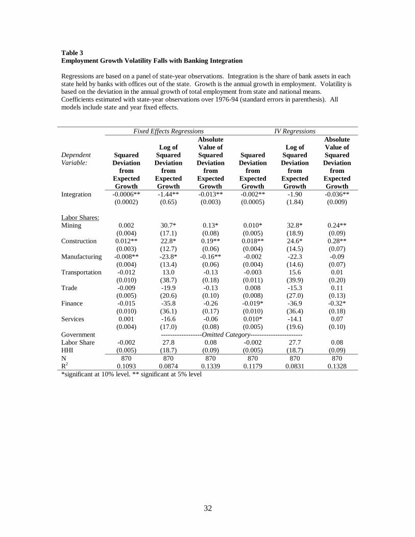
Tables 3 and 4 report the estimated coefficients for the twelve specifications. For

overall employment growth, all of the estimates are negative, and five of the six are

statistically significant at the five percent level (Table 3). Integration has had, on net, a

stabilizing influence on state business volatility. In addition, the IV coefficient estimates

are much larger than the corresponding OLS estimates in all three cases, implying that

the stabilizing influence of integration is larger (if less precisely estimated) when we use

deregulation variables to parcel out the endogenous variation in integration. In fact, the

portion of integration that is orthogonal to deregulation is strongly positively related to

employment volatility (not reported), perhaps because out-of-state banking companies

opportunistically enter new states when banks in those states are facing difficulties

associated with an economic downturn. (Remember: banks enter new states by buying

their way in.)

We do not find evidence in these regressions that diversification across industries,

measured by the labor share HHI index, reduces volatility, as one might expect. There is

very little time-series variation in this index, however, making it difficult to measure its

coefficient in the fixed effects models. If we drop the state fixed effects and estimate the

17 But other important changes occurred during the 1980s, such as rapid adoption of sophisticated financialmodels and increased use of securitization, not just for residential mortgages but also for consumer loans,commercial real estate loans and even commercial and industrial loans (Mishkin and Strahan, 1999). Thesenew technologies seem to have increased the efficient scale in banking and may be responsible, in part, forgreater integration. For an exhaustive review of the causes and consequences of financial consolidation inthe U.S., see Berger, Demsetz and Strahan (1999).

19

19

model with random effects instead, the labor share HHI does enter the regression with a

positive and statistically significant coefficient (not reported).

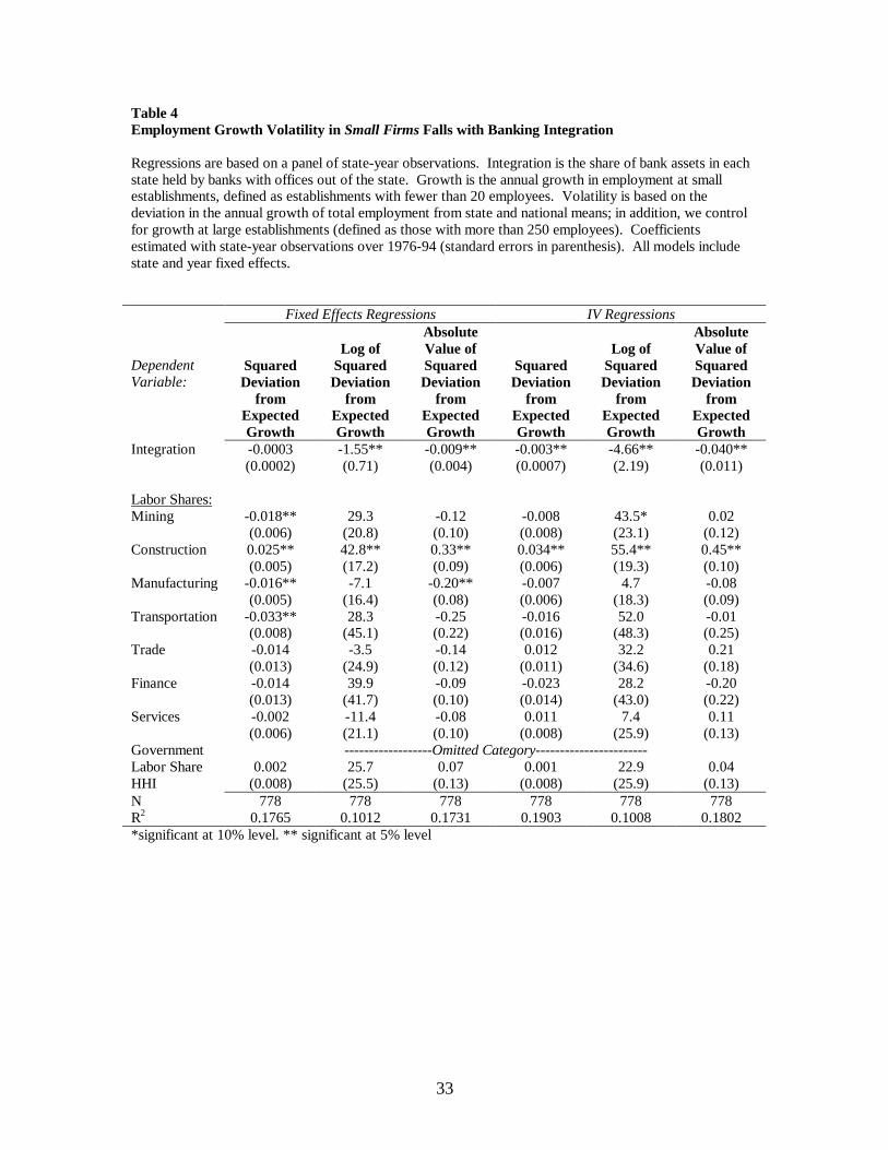
We also find declines in employment growth volatility at small firms, where we

expect the influence of banking, and hence banking integration, to be most important

(Table 4). Here, we find a statistically significant effect of banking integration on

volatility in five of our six specifications. Moreover, the declines in volatility are larger

for the small firms than for overall employment in all of the IV specifications.

The IV estimates for both overall and small-firm employment imply a substantial

stabilizing benefit from integrating bank assets across states. The share of integrated

bank assets rose from around 10 percent in 1976 to around 60 percent in 1994; the

reduced form model (not reported) suggests that about one-half of this increase can be

attributed to interstate deregulation, or an increase in integration of 25 percent. Based on

the coefficient from the IV model, this 25 percent increase in integrated bank assets

reduced the absolute deviation of overall state employment growth by 0.9 percent (Table

3, column 6). This decline is very large relative to the mean (1.3 percent) and standard

deviation (1.2 percent) over the whole sample. For small-firm employment, the IV

estimate suggests that the 25 percent increase in integrated bank assets led to a drop in

volatility of 1 percent (Table 4, column 6).

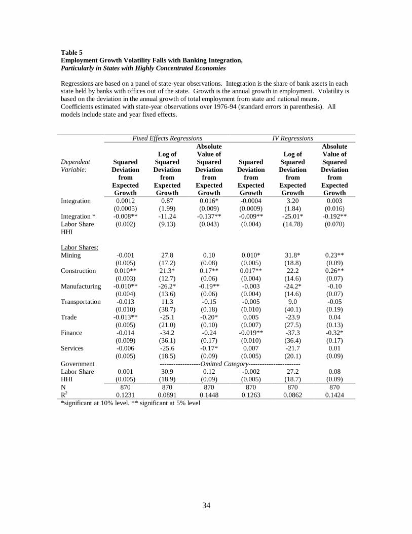
Table 5 reports a slightly more complex model in which we interact the labor

share HHI index with the banking integration variable. We find that banking integration

matters more when a state specializes in one or a few broad industries. In states with a

well-diversified economy (i.e. states with many industries), we should not expect banking

integration to matter very much. A well-diversified state will have well-diversified (unit)

20

20

banks too, thus reducing the potential benefit of integration. In contrast, in a state that

relies heavily on one or two sectors, banks constrained to operating only there will also

rely on those one or two sectors. Integrating these banks ought to have greater benefits,

and the results suggest that it has. To understand the magnitude of this interaction,

consider two states, one with labor share HHI one standard deviation below average, and

the other with labor share HHI one standard deviation above average. The poorly

diversified state’s growth volatility (absolute value of growth deviation) would decline by

1.2 percent following the 25 increase in integration, while the well-diversified state’s

growth volatility would decline by just 0.6 percent (Table 5, column 6).

IV.2 Integration Weakens the Links between Bank Capital and Business Activity

The model laid out in Section 2 suggests that the stabilizing effects of integration

occur because of better diversification against bank capital shocks. If capital falls in state

A, affiliated banks in state B will be happy to supply more to take advantage of good

investment opportunities. Integration means that more banks in state A have affiliates

outside the state. Therefore, integration ought to weaken the link between bank capital

growth within a state and growth in both lending and business activity in that state.

To test this idea, we estimate how local employment growth, as well as loan

growth by local banks, correlates with local capital growth, and how this correlation has

changed in response to banking integration. To be precise, we regress state employment

growth (total and small firm), aggregate growth of commercial and industrial loans, and

aggregate growth of commercial real estate loans on: the growth in total bank capital held

at banks in the state, our measure of banking integration, and an interaction between

21

21

banking integration and bank capital growth.18 If the model is right, capital growth ought

to be highly correlated with both employment growth and loan growth prior to banking

integration, but much less correlated after. That is, the coefficient on the interaction term

ought to be negative.19 (In all of the specifications, we also include time and state fixed

effects.)

The results in Table 6 suggest that as states integrate, local bank capital becomes

much less correlated with measures of overall economic activity (employment growth)

and with lending by banks in the state.20 For example, prior to banking integration, a one

standard deviation decline in bank capital growth (a decline of 8.4 percent) was

associated with a reduction in employment growth of 1.4 percent (Panel A, column 1).

With full banking integration, the model suggests that a one standard deviation decline in

bank capital growth would be associated with a slight increase in employment growth.

We find similar effects of banking integration on employment growth at small firms;

bank capital matters a lot prior to integration but much less after.

Table 6 also shows that the link between bank capital and loan growth to

businesses declined sharply after banking integration. Here, the effects are even more

striking. Prior to integration, we estimate a coefficient on capital that is not statistically

significantly different from one. Capital growth and loan growth moved one-for-one; if

18 The data on commercial and industrial loans only become available after 1984, so these regressions havefewer observations than the others.19 The approach is somewhat similar to studies testing whether bank lending becomes less sensitive to theirown capital or to the supply of local deposits if the bank is part of a multi-bank holding company. Our testis essentially an aggregated version of these tests. We ask: does a bank system become less sensitive to itsown financial health when it is integrated with banks outside the system? See Houston and James (1997)and Jayaratne and Morgan (1999).20 We have also estimated these regressions using IV, where an instrument for integration is constructedfrom a indicator variable equal to one after state-level interstate banking reform and a continuous variableequal to the log of the number of years elapsed since reform. These results are similar to those reported inTable 5.

22

22

capital growth fell by one percent in a year, so did loan growth. In contrast, the

coefficient on capital growth falls almost to zero after full integration. A zero coefficient

makes sense in a fully integrated banking system – a banking system in which all of the

state’s banking assets are owned by companies operating in other states too – because

lending will be determined by the presence or absence of good projects, not the presence

or absence of local capital. Capital can be imported or exported at low cost once banks

integrate.

V. Conclusions

The U.S. used to have 50 little banking systems, one in every state. With

deregulation over the last twenty-five years, we have moved toward a more integrated,

national banking system with holding companies operating banks in many different

states. As a theoretical matter, the impact of cross-state banking on business volatility is

ambiguous, as integration immunizes borrowers from shocks to their own banks but

exposes them to shocks in other states. Empirically, integration seems stabilizing on net;

employment growth fluctuations in a state diminish as its banks commingle with other

states’ banks. The balkanized business of U.S banking before the mid-1980s was, in all

likelihood, a source of state business volatility. Integration promotes convergence in the

business cycles across states; deviations in employment growth from the national average

tend to fall as integration increases. State business cycles are becoming smaller, in other

words, but more alike. As the French say: the more things change, the more they stay the

same.

23

23

References

Bernanke, B., and M. Gertler, “Banking and Macroeconomic Equilibrium,” in NewApproaches to Monetary Economics, W. Barnett and K. Singleton, eds. (NewYork and Melbourne: Cambridge University Press, 1987).

Berger, Allen N., Rebecca S. Demsetz, and Philip E. Strahan (1999), “The Consolidation of theFinancial Services Industry: Causes, Consequences, and Implications for the Future,”Journal of Banking and Finance, Vol. 23, No. 3-4, 135-194.

Clark, T., and E. Wincoop, “Borders and Business Cycles,” Forthcoming in Journal ofInternational Economics, 2000.

Demsetz, Rebecca S. and Philip E. Strahan (1997), “Size, Diversification and Risk at US BankHolding Companies,” Journal of Money, Credit and Banking, Vol. 29, 300-13.

Feldstein, Martin, 1997, EMU and International Conflict, Foreign Affairs, 76, 60-73.

Garcia Blandon, Josep, Cross-border Banking in Europe: An EmpiricalInvestigation, Working paper No 509, October 2000, Universitat PompeuFabra. 2000.

Holmstrom, B., and J. Tirole, “Financial Intermediation, Loanable Funds, and the RealSector,” Quarterly Journal of Economics, CXII (1997), 663-691.

Houston, Joel, Christopher James, and David Marcus, 1997, “Capital Market Frictionsand the Role of Internal Capital Markets in Banking,” Journal of FinancialEconomics 46, 135-164.

Jayaratne, Jith and Donald P. Morgan, 1999, “Capital Market Frictions and DepositConstraints on Banks,” Journal of Money, Credit and Banking.

Jayaratne, Jith and Philip E. Strahan (1996), “The Finance-Growth Nexus: Evidence from BankBranch Deregulation,” Quarterly Journal of Economics, Vol. 111, 639-670.

_____ (1998), “Entry Restrictions, Industry Evolution, and Dynamic Efficiency: Evidence fromCommercial Banking, The Journal of Law and Economics, Vol. XL1 (1), 239-273.

Kane, Edward (1996), “De Jure Interstate Banking: Why Only Now?,” Journal of Money, Creidt,and Banking, Vol. 28, May, 141-161.

Kroszner, Randall S. and Philip E. Strahan (1999), “What Drives Deregulation: Economics andPolitics of the Relaxation of Bank Branching Restrictions,” Quarterly Journal ofEconomics, Vol. 114, No. 4, 1437-67.

McPherson, S., and C. Waller, “Do Local Banks Matter for the Local Economy? InSearch of a Regional Credit Channel,” Forthcoming in InternationalMacroeconomics, G. Mess and E. Wincoop, eds., (Cambridge University Press,1999).

24

24

Spong, Kenneth (2000). Banking Regulation: Its Purposes, Implementation, and Effects. FederalReserve Bank of Kansas City, Kansas City: MO.

Stockman, A., and L. Tesar, “Tastes and Technology in a Two-Country Model of theBusiness Cycle: Explaining International Comovements,” American EconomicReview, LXXXV (1995), 168-185.

Williamson, S., “Bank Failures, Financial Restrictions, and Aggregate Fluctuations:Canada and the United States, 1870-1913,” Federal Reserve Bank of MinneapolisQuarterly Review, XIII (1989), 20-40.

Williamson, S., “Restrictions on Financial Intermediaries and Implications for AggregateFluctuations: Canada and the United States 1870-1913,” in NBERMacroeconomics Annual: 1989, O. Blanchard and S. Fischer, eds. (Cambridge,Mass. And London: MIT Press, 1989).

25

Appendix: Comparative statics in the HT Model with unit and interstate

banking

Equilibrium with unit banking

With unit banking and assuming γ exogenous, equilibrium on the uninformed

capital market in state 1 obtains when

(1a) ( ) uuH KupcbRKuKmKfp 1111 /)()( ⋅=∆+−++ γ .

Solving this equation, we obtain the equilibrium quantity of uninformed capital

attracted by firms in state 1

(2a) γ⋅∆+∆⋅−+

+∆⋅+−−=ppRcbp

KmKfpRcbpKuH

Hu

)())(( 11

1 .

Equilibrium in state 2 can be defined in a similar way.

Equilibrium with interstate banking

Interstate banking changes the equilibrium in the following way. Assuming

capital can move freely across states, the shares 1π and (1- 1π ) of aggregate informed

capital Km1+Km2 invested in each state adjust endogenously to equalize the return on

informed capital across states. When the share of informed capital invested in each state

is endogenous, equilibrium in the uninformed capital market under interstate banking is

defined by

(3a) ( )( ) iiH KupcbRKuKmKmKfp 112111 /)()( ⋅=∆+−+++ γπ

(4a) ( )( ) iiH KupcbRKuKmKmKfp 222112 /)())(1( ⋅=∆+−++−+ γπ .

The equilibrium rate of return on the bank capital market is:

26

(5a) ( ) ( )))(1(/)(/ 21122111 KmKmpKcpKmKmpKcp HH +−∆⋅⋅=+⋅∆⋅⋅= ππβ .

With iKuKmKmKfK 121111 )( +++= π and iKuKmKmKfK 221122 ))(1( ++−+= π

Solving the system of equations defined by (3a)-(5a), we obtain the equilibrium

quantities attracted by firms in each state and the share of informed capital invested in

each state:

(6a) ( ) )()())((

21

121211 KfKfppRcbp

KfKmKmKfKfpRcbpKuH

Hi

+⋅∆+∆⋅−++++∆⋅+−−=

γ

(7a) ( ) )()())((

21

221212 KfKfppRcbp

KfKmKmKfKfpRcbpKuH

Hi

+⋅∆+∆⋅−++++∆⋅+−−=

γ

(8a) 21

11 KfKf

Kf+

=π

Comparative statics

To get the intuition for proposition 1 and 2, we compare the equilibrium condition for

unit banking (1a) and for interstate banking in state 1 (3a), after substitution of 1π by its

reduced-form solution in (8a). The equilibrium conditions for the two regimes are plotted

in figure 1.

Let’s first consider the bank capital crunch. With unit banking, the reduction in the

pledgeable income is proportional to the reduction of 1Km . With interstate banking, by

contrast, the reduction in the pledgeable income is less than proportional to the reduction

of 1Km , since 1π is smaller than unity. Graphically, this implies a smaller reduction of

the intercept of the curve representing the pledgeable income. Because the pledgeable

income decreases less with interstate banking following a bank capital crunch, we also

have a smaller reduction in the amount of uninformed capital that can be attracted by

firms.

27

A similar mechanism is at work for the collateral squeeze. With unit banking, the

reduction in pledgeable income is proportional to the reduction of 1Kf . With interstate

banking, by contrast, the reduction in pledgeable income is more than proportional to the

reduction of 1Kf , because the share of informed capital 1π invested in state 1 – which

depends on the amount of capital available in the two states – also decreases following a

decrease of 1Kf . Graphically, this implies a larger reduction of the intercept of the curve

representing the pledgeable income. Because the pledgeable income decreases more with

interstate banking following a collateral squeeze, we also have a larger reduction in the

amount of uninformed capital that can be attracted by firms.

Capital crunch: proof of proposition 1

For the unit banking case, the derivative of 1Ku with respect to 1Km is

Impact on the availability of uninformed capital

For the unit banking case, the derivative of 1Ku with respect to 1Km is

γ⋅∆+∆⋅−+∆⋅+−−=

∂∂

ppRcbppRcbp

KmKu

H

Hu

)()(

1

1

11 KmKu u ∂∂ is positive. The numerator is positive because the positiveness of the

payment promised to uninformed investors, 0)/)(( >∆+−= pcbRKRm , implies

0)( >∆⋅+−− pRcbpH . The denominator is also positive, because the return on

uninformed capital γ has to be larger than the pledgeable expected income

)/)(( pcbRpH ∆+− to have an interior solution for 1Ku (see HT, p. 682). For the

interstate banking case, the derivative of 1Ku with respect to 1Km is

( )γ⋅∆+∆⋅−+∆⋅+−−=

∂∂

ppRcbppRcbp

KmKu

H

Hi

)(2)(

1

1

under the above mentioned symmetry conditions.

28

11 KmKu u ∂∂ is twice as large as 11 KmKu i ∂∂ .¦

Impact on the availability of informed capital

For the unit banking case, the derivative of 1Km with respect to itself is equal to unity.

For the interstate banking case, the quantity of informed capital attracted by firms in state

1 is equal to )( 211 KmKm +π with 21

11 KfKf

Kf+

=π . The derivative of this quantity with

respect to 1Km is

21)(

1

211 =∂

+∂Km

KmKmπ


1211 /)( KmKmKm ∂+∂π is smaller than unity. ¦

Collateral squeeze: proof of proposition 2


For the unit banking case, the derivative of 1Ku with respect to 1Kf is

γ⋅∆+∆⋅−+∆⋅+−−=

∂∂

ppRcbppRcbp

KfKu

H

Hu

)()(

1

1 .

11 KfKu u ∂∂ is positive.

For the interstate banking case, the derivative of 1Ku with respect to 1Kf is equal to

( )γ⋅∆+∆⋅−++∆⋅+−−=

∂∂

ppRcbpKfKmKfpRcbp

KfKu

H

Hi

)(2)2)((

1

11

1

1

29

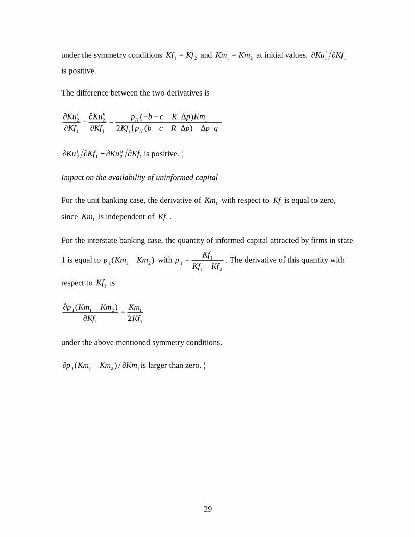
under the symmetry conditions 21 KfKf = and 21 KmKm = at initial values. 11 KfKu i ∂∂

is positive.

The difference between the two derivatives is

( )γ⋅∆+∆⋅−+∆⋅+−−=

∂∂−

∂∂

ppRcbpKfKmpRcbp

KfKu

KfKu

H

Hui

)(2)(

1

1

1

2

1

2

1212 KfKuKfKu ui ∂∂−∂∂ is positive. ¦


For the unit banking case, the derivative of 1Km with respect to 1Kf is equal to zero,

since 1Km is independent of 1Kf .

For the interstate banking case, the quantity of informed capital attracted by firms in state

1 is equal to )( 211 KmKm +π with 21

11 KfKf

Kf+

=π . The derivative of this quantity with

respect to 1Kf is

1

1

1

211

2)(

KfKm

KfKmKm =

∂+∂π


1211 /)( KmKmKm ∂+∂π is larger than zero. ¦

30

Table 1State-Specific Business Cycle Shocks have Fallen as Integration Has Risen

We decompose employment growth and personal income growth, for which we have a longer time series,in state j in year t as follows:

Yj,t=aj+bt+ej,t

Where aj is the state-specific average growth rate over the period; bt is the aggregate shock to growth attime t; ej,t is the time t shock to growth that is specific to circumstances in state j. We estimate theseregressions separately over 5 non-overlapping periods (i.e. the state fixed effect is allowed to be differentover each of the 5 periods).

Panel A: Employment Growth

Period

Root MSE OfState-Specific

Shock toEmploymentGrowth (ej,t)

Average BankIntegration

1977-1981 Pre-Interstate Banking 2.4% 14%1982-1985 Transition 2.2% 26%1986-1989 Transition 1.9% 46%1990-1993 Transition 1.6% 53%1994-1997 Post-Interstate Banking 1.1% 59%

Panel B: Personal Income Growth

Period

Root MSE OfState-Specific

Shock toEmploymentGrowth (ej,t)

Average BankIntegration

1962-1966 Pre-Interstate Banking 3.5% Low*

1967-1971 Pre-Interstate Banking 2.0% Low1972-1976 Pre-Interstate Banking 3.9% Low1977-1981 Pre-Interstate Banking 3.0% 14%1982-1985 Transition 2.0% 26%1986-1989 Transition 1.9% 46%1990-1993 Transition 1.3% 53%1994-1997 Post-Interstate Banking 1.5% 59%1998-2000 Post-Interstate Banking 1.0% High*

*Integration equals the share of banking assets in a state owned by a multi-state bank holding company.We do not have the data to construct this integration measure before 1976 or after 1994. (The figure for the1994-1997 period is the average for 1994.) Note that interstate integration continued after 1994 due tocross-state consolidation such as the merger of Bank of America (a west coast bank holding company) andNationsBank (an southeast bank holding company) in 1998. We cannot construct our measure ofintegration after 1994 because bank holding companies began to consolidate their holding of bank assetsacross state lines in 1995. We believe that the integration figure would be higher than 59% during the lastyears in this table, however.

31

Table 2Bank Integration, Business Volatility and State Labor ShareSummary Statistics

Statistics calculated using state-year observations. Integration is the share of bank assets in each state heldby banks with offices out of the state. Growth is the annual growth in employment or small firmemployment, where a firm is defined as small if it has fewer than 20 employees. Volatility is based on thedeviation in the annual growth of total employment or small firm employment (firms with fewer than 20employees) from state and national means. To construct this deviation for small firms, we also control foremployment growth at large firms (firms with more than 250 employees).

N MeanStandardDeviation

A. Integration 931 0.34 0.28

B. EmploymentEmployment Growth 931 0.023 0.023Squared Deviation from Expected Growth 931 0.0003 0.0007Log of Squared Deviation from Expected Growth 931 -9.66 2.40Absolute Value of Squared Deviation from Expected Growth 931 0.013 0.012

C. Small-Firm Employment (< 20 Employees)Employment Growth 823 0.023 0.026Squared Deviation from Expected Growth 823 0.0004 0.0008Log of Squared Deviation from Expected Growth 823 -9.58 2.46Absolute Value of Squared Deviation from Expected Growth 823 0.014 0.013

D. Labor SharesMining 870 0.013 0.018Construction 870 0.048 0.014Manufacturing 870 0.194 0.112Transportation 870 0.055 0.012Trade 870 0.229 0.038Finance 870 0.054 0.013Services 870 0.221 0.060Government 870 0.188 0.048Labor Share HHI (Sum of Squared Shares) 870 0.203 0.058

32

Table 3Employment Growth Volatility Falls with Banking Integration

Regressions are based on a panel of state-year observations. Integration is the share of bank assets in eachstate held by banks with offices out of the state. Growth is the annual growth in employment. Volatility isbased on the deviation in the annual growth of total employment from state and national means.Coefficients estimated with state-year observations over 1976-94 (standard errors in parenthesis). Allmodels include state and year fixed effects.

Fixed Effects Regressions IV Regressions

DependentVariable:

SquaredDeviation

fromExpectedGrowth

Log ofSquaredDeviation

fromExpectedGrowth

AbsoluteValue ofSquaredDeviation

fromExpectedGrowth

SquaredDeviation

fromExpectedGrowth


fromExpectedGrowth


fromExpectedGrowth

Integration -0.0006**(0.0002)

-1.44**(0.65)

-0.013**(0.003)

-0.002**(0.0005)

-1.90(1.84)

-0.036**(0.009)

Labor Shares:Mining 0.002

(0.004)30.7*(17.1)

0.13*(0.08)

0.010*(0.005)

32.8*(18.9)

0.24**(0.09)

Construction 0.012**(0.003)

22.8*(12.7)

0.19**(0.06)

0.018**(0.004)

24.6*(14.5)

0.28**(0.07)

Manufacturing -0.008**(0.004)

-23.8*(13.4)

-0.16**(0.06)

-0.002(0.004)

-22.3(14.6)

-0.09(0.07)

Transportation -0.012(0.010)

13.0(38.7)

-0.13(0.18)

-0.003(0.011)

15.6(39.9)

0.01(0.20)

Trade -0.009(0.005)

-19.9(20.6)

-0.13(0.10)

0.008(0.008)

-15.3(27.0)

0.11(0.13)

Finance -0.015(0.010)

-35.8(36.1)

-0.26(0.17)

-0.019*(0.010)

-36.9(36.4)

-0.32*(0.18)

Services 0.001(0.004)

-16.6(17.0)

-0.06(0.08)

0.010*(0.005)

-14.1(19.6)

0.07(0.10)

Government ------------------Omitted Category-----------------------Labor ShareHHI

-0.002(0.005)

27.8(18.7)

0.08(0.09)

-0.002(0.005)

27.7(18.7)

0.08(0.09)

N 870 870 870 870 870 870R2 0.1093 0.0874 0.1339 0.1179 0.0831 0.1328*significant at 10% level. ** significant at 5% level

33

Table 4Employment Growth Volatility in Small Firms Falls with Banking Integration

Regressions are based on a panel of state-year observations. Integration is the share of bank assets in eachstate held by banks with offices out of the state. Growth is the annual growth in employment at smallestablishments, defined as establishments with fewer than 20 employees. Volatility is based on thedeviation in the annual growth of total employment from state and national means; in addition, we controlfor growth at large establishments (defined as those with more than 250 employees). Coefficientsestimated with state-year observations over 1976-94 (standard errors in parenthesis). All models includestate and year fixed effects.


DependentVariable:

SquaredDeviation

fromExpectedGrowth


fromExpectedGrowth


fromExpectedGrowth

SquaredDeviation

fromExpectedGrowth


fromExpectedGrowth


fromExpectedGrowth

Integration -0.0003(0.0002)

-1.55**(0.71)

-0.009**(0.004)

-0.003**(0.0007)

-4.66**(2.19)

-0.040**(0.011)

Labor Shares:Mining -0.018**

(0.006)29.3

(20.8)-0.12(0.10)

-0.008(0.008)

43.5*(23.1)

0.02(0.12)


42.8**(17.2)

0.33**(0.09)

0.034**(0.006)

55.4**(19.3)

0.45**(0.10)


-7.1(16.4)

-0.20**(0.08)

-0.007(0.006)

4.7(18.3)

-0.08(0.09)

Transportation -0.033**(0.008)

28.3(45.1)

-0.25(0.22)

-0.016(0.016)

52.0(48.3)

-0.01(0.25)

Trade -0.014(0.013)

-3.5(24.9)

-0.14(0.12)

0.012(0.011)

32.2(34.6)

0.21(0.18)

Finance -0.014(0.013)

39.9(41.7)

-0.09(0.10)

-0.023(0.014)

28.2(43.0)

-0.20(0.22)

Services -0.002(0.006)

-11.4(21.1)

-0.08(0.10)

0.011(0.008)

7.4(25.9)

0.11(0.13)


0.002(0.008)

25.7(25.5)

0.07(0.13)

0.001(0.008)

22.9(25.9)

0.04(0.13)


34

Table 5Employment Growth Volatility Falls with Banking Integration,Particularly in States with Highly Concentrated Economies

Regressions are based on a panel of state-year observations. Integration is the share of bank assets in eachstate held by banks with offices out of the state. Growth is the annual growth in employment. Volatility isbased on the deviation in the annual growth of total employment from state and national means.Coefficients estimated with state-year observations over 1976-94 (standard errors in parenthesis). Allmodels include state and year fixed effects.


DependentVariable:

SquaredDeviation

fromExpectedGrowth


fromExpectedGrowth


fromExpectedGrowth

SquaredDeviation

fromExpectedGrowth


fromExpectedGrowth


fromExpectedGrowth

Integration 0.0012(0.0005)

0.87(1.99)

0.016*(0.009)

-0.0004(0.0009)

3.20(1.84)

0.003(0.016)

Integration *Labor ShareHHI

-0.008**(0.002)

-11.24(9.13)

-0.137**(0.043)

-0.009**(0.004)

-25.01*(14.78)

-0.192**(0.070)

Labor Shares:Mining -0.001

(0.005)27.8

(17.2)0.10

(0.08)0.010*(0.005)

31.8*(18.8)

0.23**(0.09)


21.3*(12.7)

0.17**(0.06)

0.017**(0.004)

22.2(14.6)

0.26**(0.07)


-26.2*(13.6)

-0.19**(0.06)

-0.003(0.004)

-24.2*(14.6)

-0.10(0.07)

Transportation -0.013(0.010)

11.3(38.7)

-0.15(0.18)

-0.005(0.010)

9.0(40.1)

-0.05(0.19)

Trade -0.013**(0.005)

-25.1(21.0)

-0.20*(0.10)

0.005(0.007)

-23.9(27.5)

0.04(0.13)

Finance -0.014(0.009)

-34.2(36.1)

-0.24(0.17)

-0.019**(0.010)

-37.3(36.4)

-0.32*(0.17)

Services -0.006(0.005)

-25.6(18.5)

-0.17*(0.09)

0.007(0.005)

-21.7(20.1)

0.01(0.09)


0.001(0.005)

30.9(18.9)

0.12(0.09)

-0.002(0.005)

27.2(18.7)

0.08(0.09)


35

Table 6Integration Lowers the Correlation between Employment, Loan Growth and Bank Capital

Reported are fixed effects regression coefficients and standards errors (in parenthesis) estimated for panelof 48 states and D.C. The dependent variable and associated estimation periods are indicated at the top ofeach column. Bank capital growth is the annual growth rate of total capital held by all banks headquarteredin each state. Integration is the share of bank assets in each state held by banks with offices out of the state.All regressions include state and year fixed effects (not reported).

Panel A: Employment Growth

Dependent variables: Employment growth(1976-94)

Small-firm employment growth(1978-94)

Bank Capital Growth 0.162**(0.014)

0.206**(0.016)

Integration 0.020**(0.004)

0.030**(0.005)

Bank Capital Growth xIntegration

-0.188**(0.021)

-0.239**(0.024)

R2 0.542 0.604N 882 823

F-test that Bank Capital +Capital x Integration = 0(p-value)

5.50(0.02)

7.11(0.01)

Panel B: Loan Growth

Dependent variables:C&I loan growth

(1978-1994)

Commercial real estate loangrowth

(1985-1994)

Bank Capital Growth 0.944**(0.108)

1.148**(0.097)

Integration 0.091*(0.047)

0.094**(0.029)

Bank Capital Growth xIntegration

-0.780**(0.159)

-0.994**(0.149)

R2 0.444 0.426N 490 882

F-test that Bank Capital +Capital x Integration = 0(p-value)

4.73(0.03)

3.92(0.05)

*significant at 10% level. ** significant at 5% level

36

37

Chart 1: Cross-Nation Bank Liabilities in Europe (1988 and 1997)

Share o f Cross-Border L iab i l i t i es as a % o f Tota l L iab i l i t i es

0.00

10.00

20.00

30.00

40.00

50.00

60.00

70.00

80.00

90.00

Austria

Belgium

Denmark

Finlan

d

Franc

e

German

y

Greec

e

Icelan

d

Irelan

dIta

ly

Luxe

mbourg

Netherl

ands

Norway

Portug

al

Spain

Sweden

Switzer

land

United

King

dom

%

1 9 8 8 1 9 9 7

Source: Bank of International Settlements

Chart2: Cross-State Banking Waves

% of out-of-state bank assets (median for year)in

tegr

atio

n

year1975 1977 1979 1981 1983 1985 1987 1989 1991 1993 1995 1997

0

.1

.2

.3

.4

.5

.6

.7

Interstate banking agreements occurred in waves between 1982 and 1993. States were grouped by theyear that they entered into an agreement. Plotted for each wave is the median share of out-of-statebanking assets for states in each wave.

ο: 1982-1984 wave∆: 1985-1987 wave: : 1988-1990 wave : 1991-1993 wave

Documents

Bank Integration and Business Volatility