Commodity Price Volatility and World Market Integration

COMMODITY PRICE VOLATILITY AND WORLD MARKET

INTEGRATION SINCE 1700

David S. Jacks, Kevin H. O’Rourke, and Jeffrey G. Williamson*

Abstract—Poor countries are more volatile than rich countries, and thisvolatility impedes their growth. Furthermore, commodity prices are a keysource of that volatility. This paper explores price volatility since 1700 tooffer three stylized facts: commodity price volatility has not increasedover time, commodities have always shown greater price volatility thanmanufactures, and world market integration breeds less commodity pricevolatility. Thus, economic isolation is associated with much greater com-modity price volatility, while world market integration is associated withless.

I. Commodity Price Volatility and Development

POOR countries are more volatile than rich countries,and an extensive literature suggests that this is bad for

growth. Ramey and Ramey (1995) and Deaton (1999; Dea-ton & Miller, 1996) were among the first to find evidencethat countries with higher volatility had lower mean growth.Their results have since been confirmed: more recent anddetailed evidence (Acemoglu et al., 2003; Hnatkovska &Loayza, 2005; Fatas & Mivhov, 2006; Loayza et al., 2007)also shows that the high volatility and slow growth connec-tion seems to be especially pronounced in poor countries.Indeed, in an impressive analysis of more than sixty coun-tries between 1970 and 2003, Poelhekke and van der Ploeg(2007) find strong support for the core-periphery asymme-try hypothesis regarding volatility: that is, the volatilityinfluence is far greater in the poor periphery. Furthermore,while capricious policy and political violence can add tovolatility in poor countries, extremely volatile commodityprices ‘‘are the main reason why natural resources exportrevenues are so volatile’’ (Poelhekke & van der Ploeg 2007,p. 3), and thus why those economies are themselves so vola-tile.1

One reason for this higher volatility is that poor countriesspecialize in agricultural and mineral production. Primaryproducts, or export commodities as they are often called,experience far greater price volatility than do manufacturesor services, although this is more often assumed thandemonstrated in the literature.2 One exception to the ‘‘noevidence’’ attribute of the literature is UNCTAD (2008),which provides graphical evidence of higher price volatilityfor nonfuel commodities and petroleum than for manufac-tures between 1970 and 2008. Another is Mintz (1967),who, more than forty years ago, documented lower U.S.export price volatility for finished manufactures than forsemimanufactures, crude materials, or food between 1880and 1963. In any case, the higher volatility of commodityprices has left its mark on relative terms-of-trade experi-ence: since 1960, Latin America, South Asia, and Africahave had far higher terms-of-trade volatility than have themanufactures-exporting industrial economies—indeed, morethan three times higher (table 1).

Three questions motivate this paper. First, have primaryproduct commodities always had more volatile prices thanmanufactured goods, or did this difference arise only withmodern capitalism and the price stickiness associated withless competitive industrial organizations in manufacturingcompared with the primary sector? This view was cham-pioned by Prebisch (1950) more than fifty years ago.3 Sec-ond, has there been any secular trend in commodity pricevolatility since 1700, or has it been a constant fact of eco-nomic life? Finally, and most important, what is the rela-tionship between globalization and commodity price volati-lity? Does world market integration create more or lessprice volatility for poor commodity exporters?

International trade might be thought to encourage terms-of-trade volatility since it leads to greater specialization. Ifthe specialization is in commodities rather than manufac-tures or services, then trade will increase terms-of-tradevolatility even more. This argument holds if we make therestrictive assumption that the price volatility is the sameacross individual commodities and over time. This papertests this assumption: it explores long-run trends in the price

Received for publication February 12, 2009. Revision accepted for pub-lication January 28, 2010.

* Jacks: Simon Fraser University and NBER; O’Rourke: Trinity Col-lege Dublin and NBER; Williamson: Harvard University, University ofWisconsin, and NBER.

We acknowledge with thanks help rendered by Sambit Bhattacharyya,Chris Blattman, George Boyer, Luis Catao, Bob Gregory, Jason Hwang,Norman Loayza, Alan Matthews, Steve Poelhekke, and referees of thisREVIEW, although they are not responsible for any flaws that may remain.D.J. gratefully acknowledges the Social Sciences and HumanitiesResearch Council of Canada for research support. K.O. thanks the IrishResearch Council for the Humanities and Social Sciences and the Eur-opean Commission’s Seventh Research Framework Programme (contractnumber 225342) for their generous support. J.W. does the same for theHarvard Faculty of Arts and Science.

1 There are many reasons that poor countries face higher volatility andthat higher volatility costs them so much more in diminished growth rates.Philippe Aghion and his collaborators (2005, 2006) offer one: macroeco-nomic volatility driven by either nominal exchange rate or commodityprice movements will depress growth in poor economies with weak finan-cial institutions and rigid nominal wages, both of which characterized allpoor economies in the past even more than today. See also Aizenman andMarion (1999), Flug, Spilimbergo, and Wachtenheim (1999), Elbers,Gunning, and Kinsey (2007), and Koren and Tenreyro (2007).

2 Here are two examples. Radetzki (2008, pp. 64–66) discusses the‘‘well-known and oft-repeated’’ observation that commodity prices areextremely volatile and that ‘‘the prices of manufactures tend to be morestable.’’ He provides evidence of volatile commodity prices and discusseswhy these might be expected to be more volatile than manufacturedprices. However, he does not provide or cite empirical evidence regardingthe relative volatility of the two types of prices. Szirmai (2005, p. 543)takes the view that ‘‘prices of primary exports turn out to be no moreunstable than those of manufactured goods or capital goods,’’ again with-out providing evidence.

3 See the excellent survey in Cuddington, Ludema, and Jayasuriya(2007).

The Review of Economics and Statistics, August 2011, 93(3): 800–813

� 2011 by the President and Fellows of Harvard College and the Massachusetts Institute of Technology

volatility of individual goods rather than in the volatility ofaggregate commodity price indices, as is typical in the lit-erature.4 If international trade lowers the price volatility ofindividual commodities, then it might on balance lead to amore stable price environment overall, even for countrieswith a comparative advantage in primary products. Thus, itis strictly an empirical matter as to whether the price stabili-zation effect or the specialization effect dominates.

Why might trade lower the volatility of individual com-modity prices? The idea, of course, is that local shocks tosupply and demand are stabilized when a small domesticeconomy trades with a large world economy. Thus, whenthe world went global in the early nineteenth century(O’Rourke & Williamson, 2002), did commodity pricesbecome less volatile as small local economies became inte-grated with large world markets? When the world wentautarkic between the world wars, did commodity pricesbecome more volatile, for symmetric reasons? What aboutepisodes of war and peace? Were commodity prices morevolatile during the French wars of the late eighteenth andearly nineteenth centuries, during World War I, and duringWorld War II, than during the pro-global nineteenth centuryunder pax Britannica or the pro-global decades since 1970?What does history tell us about the commodity price volati-lity and world market integration connection?

This is hardly the first time that these questions havebeen raised, although this paper is the first time, to ourknowledge, that these questions have been confronted withextensive long-run price evidence. Persson, a scholar ofmedieval and early modern European grain markets, tells ushow central these questions were to the eighteenth-centuryphysiocrats, or what Persson calls les economistes. As far asles economistes were concerned, he wrote, ‘‘the best andfavoured remedy against price fluctuations was market inte-gration, and its prerequisite was free trade in grain’’ (1999,p. 7). Furthermore, it appears that les economistes antici-pated the modern development economist’s conclusion that

volatility is bad for growth by more than 300 years: ‘‘Oneof the accomplishments of [les economistes] was the claimthat price volatility . . . had disincentive effects on investmentand effort in agriculture . . . and that [it was] a prime causefor the distressed state of agriculture’’ (Persson, 1999, p. 7).One of the earliest of les economistes, the EnglishmanCharles Davenant, asserted in 1699 that ‘‘a stable pricewould reign if [national grain] markets were permitted totrade since price differences would make traders move grainfrom surplus to deficit regions or nations’’ (Persson, 1999,pp. 8–9, citing Davenant, 1699, p. 82).

So, were les economistes right?

II. Commodity Price Volatility since 1700: Data and

Measurement

The most recent and comprehensive paper on moderncommodity price behavior is by Poelhekke and van derPloeg (2007). The price data they used are ‘‘monthlyaverages of free-market price indices for all food, agricul-tural raw materials, minerals, ores & metals, crude petro-leum (average of Dubai/Brent/Texas equally weighted).Base year 2000 ¼ 100.’’ The source of these data isUNCTAD (2007). We use similar free market price statis-tics, except that we quote them in local markets, so thatthey reflect the impact of tariffs and embargoes. Our dataare price quotes for various items that are allocated, follow-ing UNCTAD classifications, to three groups: all food(AF), agricultural raw materials (ARM), and minerals, ores,and metals (MOM). We add a fourth group for manufac-tures or final goods (FG). These are further aggregated intoall items (ALL) and all commodities (COM).

Table 2 describes the data in greater detail. Nine sourcesproviding monthly data are listed in panel A. The famousPhiladelphia database collected by Anne Bezanson and hercollaborators (Bezanson, 1951; Bezanson, Gray, & Hussey,1935, 1936; Bezanson et al., 1954) is in four parts: 1720–1775 (19 items), 1770–1790 (25 items), 1784–1861 (133items), and 1852–1896 (100 items). The Dutch data col-lected by Posthumus (1946) and the Danish data collectedby Friis and Glamann (1958) are both much shorter (1750–1800) and smaller (49 and 29 items, respectively). The dataunderlying the Gayer, Rostow, and Schwartz (1953) Britishcommodity price index for 1790 to 1850 contain 69 items.Our historical price database is augmented with the monthlycommodity price series published by the IMF (45 series)

TABLE 1.—COMPARATIVE TERMS-OF-TRADE VOLATILITY BY REGION

IndustrializedEconomies

East Asiaand the Pacific

Latin Americaand the Caribbean

Middle Eastand North Africa

SouthAsia

Sub-SaharanAfrica

1960s 1.8 5.2 7.2 4.8 12.8 7.21970s 5.2 8.2 13.0 11.5 18.0 18.21980s 3.5 6.1 11.0 9.0 10.2 12.21990s 2.1 1.9 8.1 7.8 7.8 10.8Average 3.2 (100) 5.4 (169) 9.8 (306) 8.3 (259) 12.2 (381) 12.1 (378)

These figures are taken from Loayza et al. (2007, p. 346). Terms-of-trade volatility is calculated as the standard deviation of the logarithmic change in terms of trade over each of the four decades 1960–2000.

4 For example, Cashin and McDermott (2002) look at the behavior of abroad-based annual aggregate price index (the Economist’s industrialcommodities price index). This index is heavily weighted toward com-modities, although it also includes some basic manufactured goods. Incontrast to Cashin and McDermott, we use higher-frequency (monthly orquarterly) data where possible, use price evidence for a longer time periodand are interested not just in aggregate price volatility but in the relativeprice volatility of commodities and manufactured goods. Note, however,that later in the paper, when using the GARCH framework to model pricevolatility, we switch to using average price indices rather than individualcommodity prices.

801COMMODITY PRICE VOLATILITY AND WORLD MARKET INTEGRATION SINCE 1700

for 1980 to 2008 and UNCTAD (52 series) for 1960 to2007. As we shall see in table 6, we also have quarterly datafor U.S. export prices for 1880 to 1963.

In panel B, in table 2, two annual series are listed. TheEnglish series collected by Gregory Clark (2005) covers1700 to 1869, and contains 36 items. The Sauerbeck (1886–1917) and Statist (1930) annual British price series cover1850 to 1950 and contain 41 items. The annual series have,

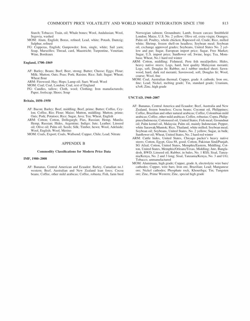
of course, lower frequency, and thus are not exactly com-parable to the monthly series, but they do offer the advan-tage of more observations from the world’s most importantnineteenth-century market, Great Britain, and, perhapsmore important, coverage of the first half of the twentieth-century. Appendix A provides full details for the commod-ities and classifications employed for the historical pricedata, and Appendix B repeats the exercise for the IMF andUNCTAD data. Finally, note that a large number of indivi-dual commodity price series have been excluded from ourdata set. In order to ensure comparable results, only goodsthat span entire sub–periods (for example, wheat in Phila-delphia from 1720 to 1775) have been incorporated into ourfinal data set.

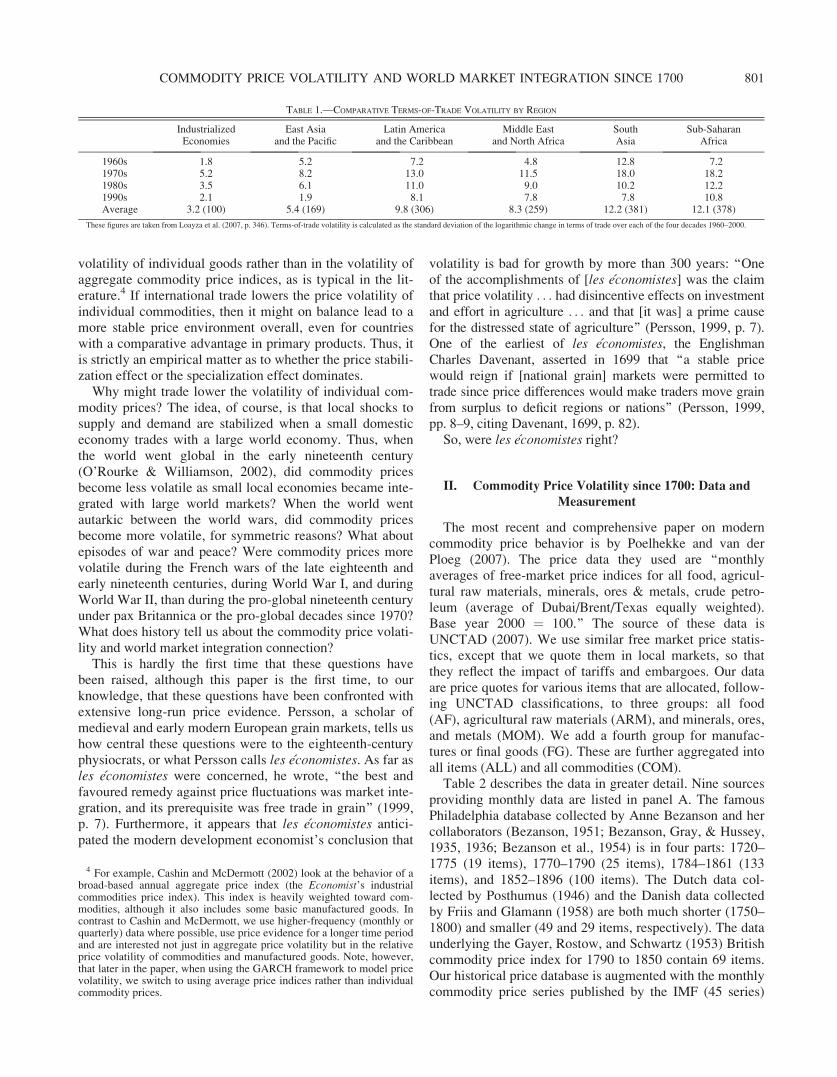
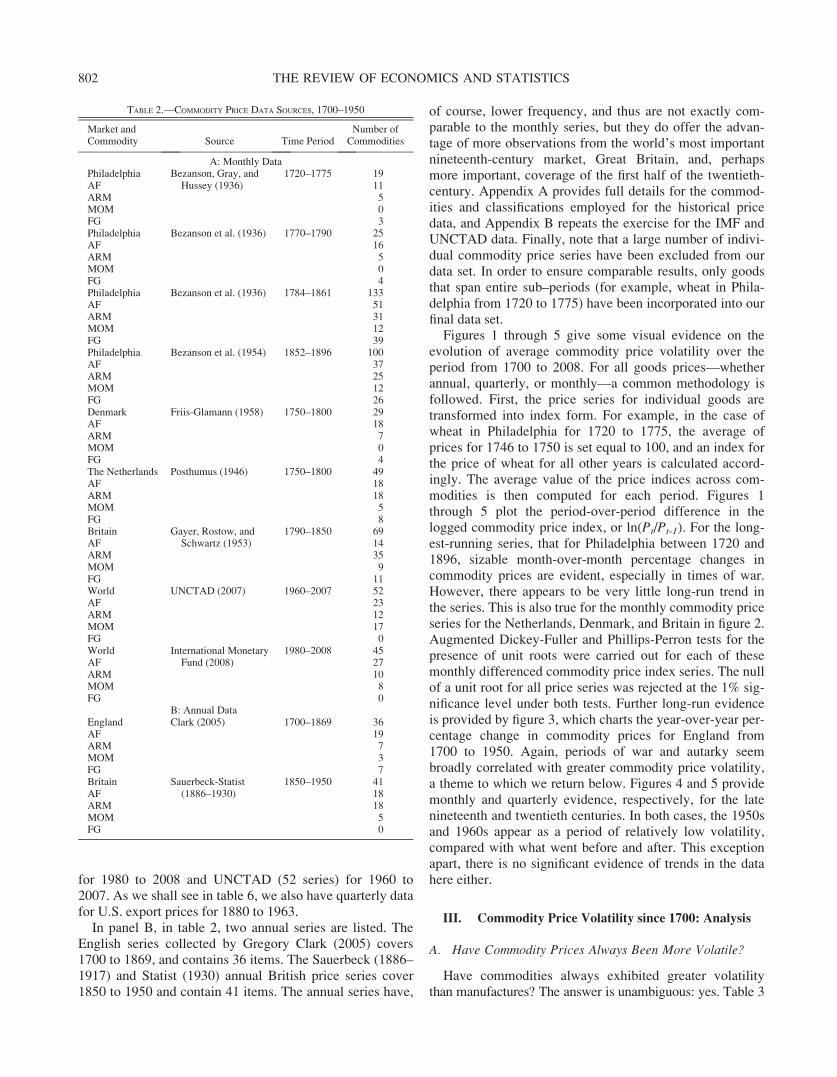
Figures 1 through 5 give some visual evidence on theevolution of average commodity price volatility over theperiod from 1700 to 2008. For all goods prices—whetherannual, quarterly, or monthly—a common methodology isfollowed. First, the price series for individual goods aretransformed into index form. For example, in the case ofwheat in Philadelphia for 1720 to 1775, the average ofprices for 1746 to 1750 is set equal to 100, and an index forthe price of wheat for all other years is calculated accord-ingly. The average value of the price indices across com-modities is then computed for each period. Figures 1through 5 plot the period-over-period difference in thelogged commodity price index, or ln(Pt/Pt-1). For the long-est-running series, that for Philadelphia between 1720 and1896, sizable month-over-month percentage changes incommodity prices are evident, especially in times of war.However, there appears to be very little long-run trend inthe series. This is also true for the monthly commodity priceseries for the Netherlands, Denmark, and Britain in figure 2.Augmented Dickey-Fuller and Phillips-Perron tests for thepresence of unit roots were carried out for each of thesemonthly differenced commodity price index series. The nullof a unit root for all price series was rejected at the 1% sig-nificance level under both tests. Further long-run evidenceis provided by figure 3, which charts the year-over-year per-centage change in commodity prices for England from1700 to 1950. Again, periods of war and autarky seembroadly correlated with greater commodity price volatility,a theme to which we return below. Figures 4 and 5 providemonthly and quarterly evidence, respectively, for the latenineteenth and twentieth centuries. In both cases, the 1950sand 1960s appear as a period of relatively low volatility,compared with what went before and after. This exceptionapart, there is no significant evidence of trends in the datahere either.

III. Commodity Price Volatility since 1700: Analysis

A. Have Commodity Prices Always Been More Volatile?

Have commodities always exhibited greater volatilitythan manufactures? The answer is unambiguous: yes. Table 3

TABLE 2.—COMMODITY PRICE DATA SOURCES, 1700–1950

Market andCommodity Source Time Period

Number ofCommodities

A: Monthly DataPhiladelphia Bezanson, Gray, and

Hussey (1936)1720–1775 19

AF 11ARM 5MOM 0FG 3Philadelphia Bezanson et al. (1936) 1770–1790 25AF 16ARM 5MOM 0FG 4Philadelphia Bezanson et al. (1936) 1784–1861 133AF 51ARM 31MOM 12FG 39Philadelphia Bezanson et al. (1954) 1852–1896 100AF 37ARM 25MOM 12FG 26Denmark Friis-Glamann (1958) 1750–1800 29AF 18ARM 7MOM 0FG 4The Netherlands Posthumus (1946) 1750–1800 49AF 18ARM 18MOM 5FG 8Britain Gayer, Rostow, and

Schwartz (1953)1790–1850 69

AF 14ARM 35MOM 9FG 11World UNCTAD (2007) 1960–2007 52AF 23ARM 12MOM 17FG 0World International Monetary

Fund (2008)1980–2008 45

AF 27ARM 10MOM 8FG 0

B: Annual DataEngland Clark (2005) 1700–1869 36AF 19ARM 7MOM 3FG 7Britain Sauerbeck-Statist

(1886–1930)1850–1950 41

AF 18ARM 18MOM 5FG 0

802 THE REVIEW OF ECONOMICS AND STATISTICS

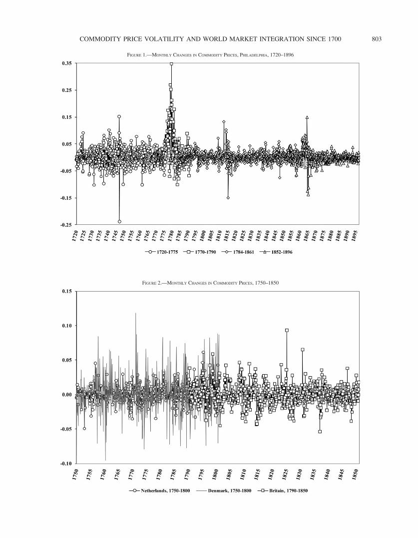
FIGURE 2.—MONTHLY CHANGES IN COMMODITY PRICES, 1750–1850

FIGURE 1.—MONTHLY CHANGES IN COMMODITY PRICES, PHILADELPHIA, 1720–1896


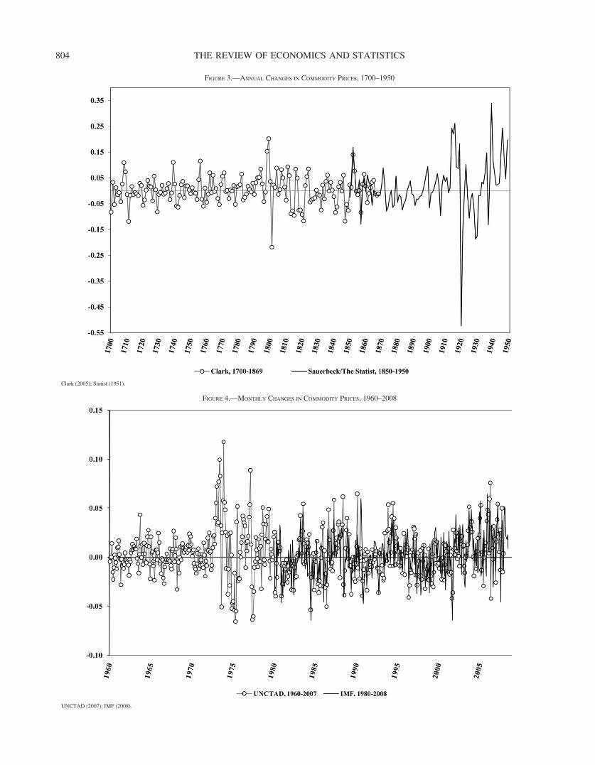
FIGURE 4.—MONTHLY CHANGES IN COMMODITY PRICES, 1960–2008

UNCTAD (2007); IMF (2008).

FIGURE 3.—ANNUAL CHANGES IN COMMODITY PRICES, 1700–1950

Clark (2005); Statist (1951).


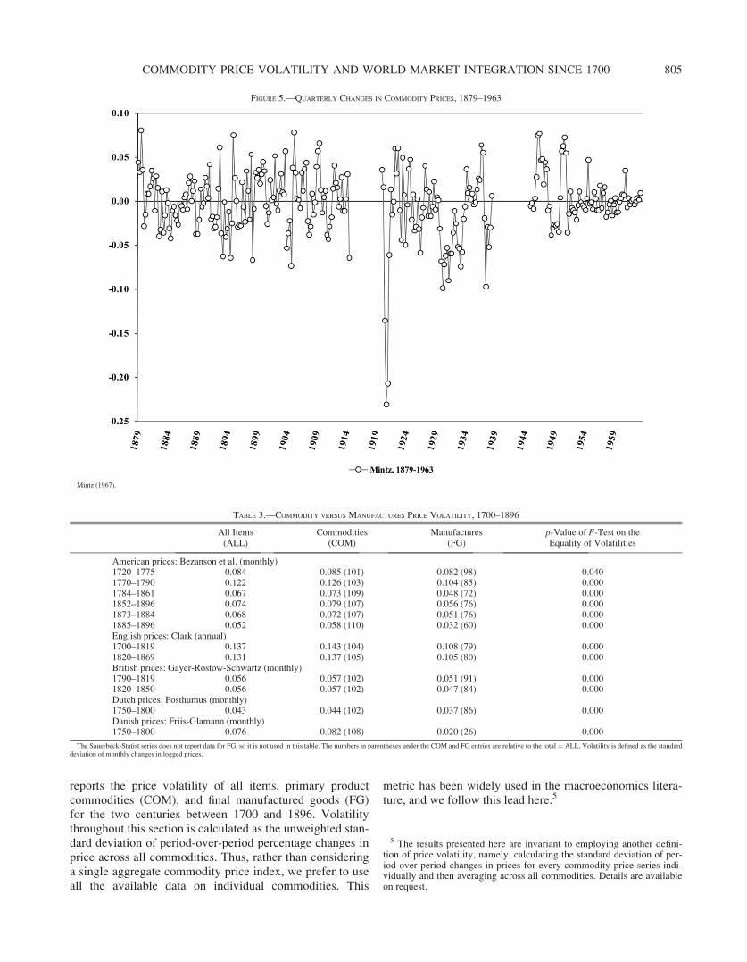
reports the price volatility of all items, primary productcommodities (COM), and final manufactured goods (FG)for the two centuries between 1700 and 1896. Volatilitythroughout this section is calculated as the unweighted stan-dard deviation of period-over-period percentage changes inprice across all commodities. Thus, rather than consideringa single aggregate commodity price index, we prefer to useall the available data on individual commodities. This

metric has been widely used in the macroeconomics litera-ture, and we follow this lead here.5

FIGURE 5.—QUARTERLY CHANGES IN COMMODITY PRICES, 1879–1963

Mintz (1967).

TABLE 3.—COMMODITY VERSUS MANUFACTURES PRICE VOLATILITY, 1700–1896

All Items(ALL)

Commodities(COM)

Manufactures(FG)

p-Value of F-Test on theEquality of Volatilities

American prices: Bezanson et al. (monthly)1720–1775 0.084 0.085 (101) 0.082 (98) 0.0401770–1790 0.122 0.126 (103) 0.104 (85) 0.0001784–1861 0.067 0.073 (109) 0.048 (72) 0.0001852–1896 0.074 0.079 (107) 0.056 (76) 0.0001873–1884 0.068 0.072 (107) 0.051 (76) 0.0001885–1896 0.052 0.058 (110) 0.032 (60) 0.000English prices: Clark (annual)1700–1819 0.137 0.143 (104) 0.108 (79) 0.0001820–1869 0.131 0.137 (105) 0.105 (80) 0.000British prices: Gayer-Rostow-Schwartz (monthly)1790–1819 0.056 0.057 (102) 0.051 (91) 0.0001820–1850 0.056 0.057 (102) 0.047 (84) 0.000Dutch prices: Posthumus (monthly)1750–1800 0.043 0.044 (102) 0.037 (86) 0.000Danish prices: Friis-Glamann (monthly)1750–1800 0.076 0.082 (108) 0.020 (26) 0.000

The Sauerbeck-Statist series does not report data for FG, so it is not used in this table. The numbers in parentheses under the COM and FG entries are relative to the total ¼ ALL. Volatility is defined as the standarddeviation of monthly changes in logged prices.

5 The results presented here are invariant to employing another defini-tion of price volatility, namely, calculating the standard deviation of per-iod-over-period changes in prices for every commodity price series indi-vidually and then averaging across all commodities. Details are availableon request.


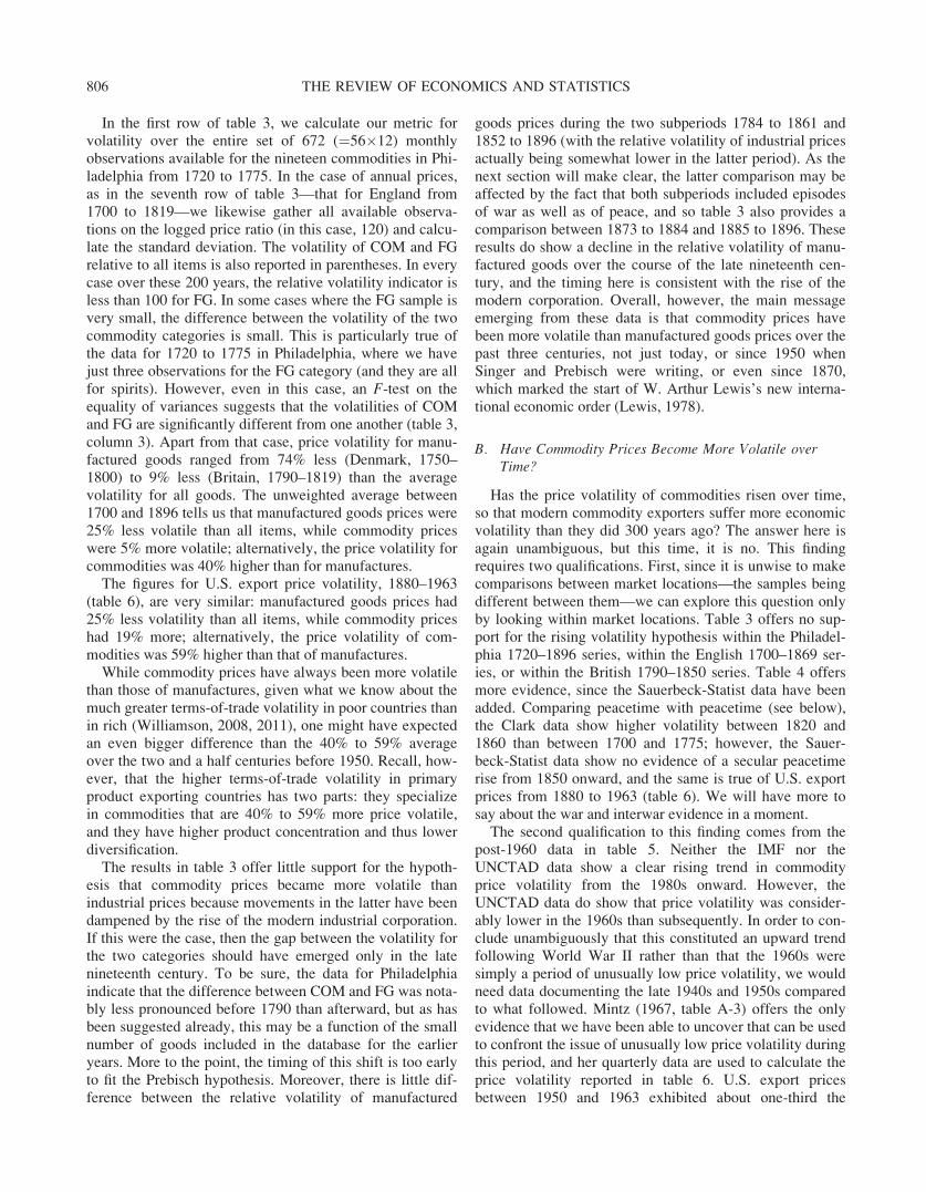
In the first row of table 3, we calculate our metric forvolatility over the entire set of 672 (¼56�12) monthlyobservations available for the nineteen commodities in Phi-ladelphia from 1720 to 1775. In the case of annual prices,as in the seventh row of table 3—that for England from1700 to 1819—we likewise gather all available observa-tions on the logged price ratio (in this case, 120) and calcu-late the standard deviation. The volatility of COM and FGrelative to all items is also reported in parentheses. In everycase over these 200 years, the relative volatility indicator isless than 100 for FG. In some cases where the FG sample isvery small, the difference between the volatility of the twocommodity categories is small. This is particularly true ofthe data for 1720 to 1775 in Philadelphia, where we havejust three observations for the FG category (and they are allfor spirits). However, even in this case, an F-test on theequality of variances suggests that the volatilities of COMand FG are significantly different from one another (table 3,column 3). Apart from that case, price volatility for manu-factured goods ranged from 74% less (Denmark, 1750–1800) to 9% less (Britain, 1790–1819) than the averagevolatility for all goods. The unweighted average between1700 and 1896 tells us that manufactured goods prices were25% less volatile than all items, while commodity priceswere 5% more volatile; alternatively, the price volatility forcommodities was 40% higher than for manufactures.

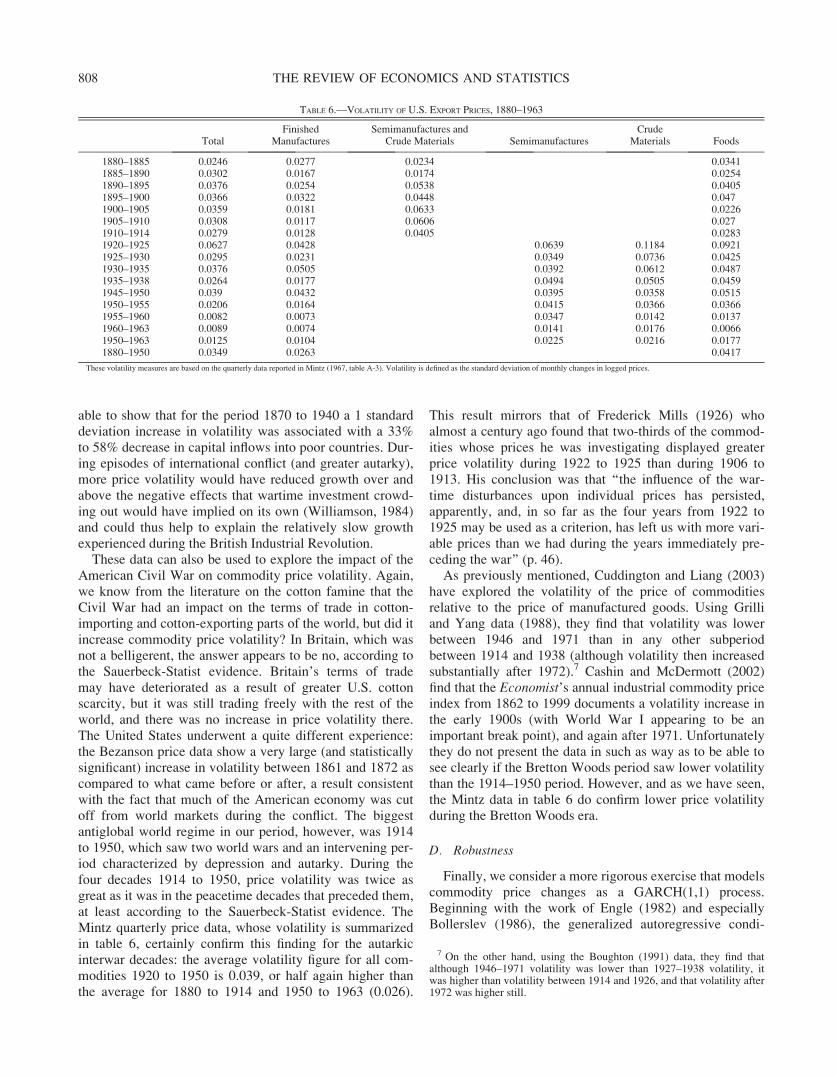
The figures for U.S. export price volatility, 1880–1963(table 6), are very similar: manufactured goods prices had25% less volatility than all items, while commodity priceshad 19% more; alternatively, the price volatility of com-modities was 59% higher than that of manufactures.

While commodity prices have always been more volatilethan those of manufactures, given what we know about themuch greater terms-of-trade volatility in poor countries thanin rich (Williamson, 2008, 2011), one might have expectedan even bigger difference than the 40% to 59% averageover the two and a half centuries before 1950. Recall, how-ever, that the higher terms-of-trade volatility in primaryproduct exporting countries has two parts: they specializein commodities that are 40% to 59% more price volatile,and they have higher product concentration and thus lowerdiversification.

The results in table 3 offer little support for the hypoth-esis that commodity prices became more volatile thanindustrial prices because movements in the latter have beendampened by the rise of the modern industrial corporation.If this were the case, then the gap between the volatility forthe two categories should have emerged only in the latenineteenth century. To be sure, the data for Philadelphiaindicate that the difference between COM and FG was nota-bly less pronounced before 1790 than afterward, but as hasbeen suggested already, this may be a function of the smallnumber of goods included in the database for the earlieryears. More to the point, the timing of this shift is too earlyto fit the Prebisch hypothesis. Moreover, there is little dif-ference between the relative volatility of manufactured

goods prices during the two subperiods 1784 to 1861 and1852 to 1896 (with the relative volatility of industrial pricesactually being somewhat lower in the latter period). As thenext section will make clear, the latter comparison may beaffected by the fact that both subperiods included episodesof war as well as of peace, and so table 3 also provides acomparison between 1873 to 1884 and 1885 to 1896. Theseresults do show a decline in the relative volatility of manu-factured goods over the course of the late nineteenth cen-tury, and the timing here is consistent with the rise of themodern corporation. Overall, however, the main messageemerging from these data is that commodity prices havebeen more volatile than manufactured goods prices over thepast three centuries, not just today, or since 1950 whenSinger and Prebisch were writing, or even since 1870,which marked the start of W. Arthur Lewis’s new interna-tional economic order (Lewis, 1978).

B. Have Commodity Prices Become More Volatile overTime?

Has the price volatility of commodities risen over time,so that modern commodity exporters suffer more economicvolatility than they did 300 years ago? The answer here isagain unambiguous, but this time, it is no. This findingrequires two qualifications. First, since it is unwise to makecomparisons between market locations—the samples beingdifferent between them—we can explore this question onlyby looking within market locations. Table 3 offers no sup-port for the rising volatility hypothesis within the Philadel-phia 1720–1896 series, within the English 1700–1869 ser-ies, or within the British 1790–1850 series. Table 4 offersmore evidence, since the Sauerbeck-Statist data have beenadded. Comparing peacetime with peacetime (see below),the Clark data show higher volatility between 1820 and1860 than between 1700 and 1775; however, the Sauer-beck-Statist data show no evidence of a secular peacetimerise from 1850 onward, and the same is true of U.S. exportprices from 1880 to 1963 (table 6). We will have more tosay about the war and interwar evidence in a moment.

The second qualification to this finding comes from thepost-1960 data in table 5. Neither the IMF nor theUNCTAD data show a clear rising trend in commodityprice volatility from the 1980s onward. However, theUNCTAD data do show that price volatility was consider-ably lower in the 1960s than subsequently. In order to con-clude unambiguously that this constituted an upward trendfollowing World War II rather than that the 1960s weresimply a period of unusually low price volatility, we wouldneed data documenting the late 1940s and 1950s comparedto what followed. Mintz (1967, table A-3) offers the onlyevidence that we have been able to uncover that can be usedto confront the issue of unusually low price volatility duringthis period, and her quarterly data are used to calculate theprice volatility reported in table 6. U.S. export pricesbetween 1950 and 1963 exhibited about one-third the


volatility that they did between 1880 and 1950. Prices ofU.S. food and finished manufactured exports exhibitedpretty much the same pattern, as did prices of U.S. semima-nufactured and crude material exports (although neither canbe documented over the full period). We also know that the1960s was a period of macroeconomic and exchange ratestability, relative to what came subsequently, and this mightperhaps explain the contrast between what is called theBretton Woods period and what followed. Indeed, Cudding-ton and Liang (2003) show that over the period 1880 to1996, there was greater volatility in the relative price ofcommodities to manufactured goods during periods of float-ing exchange rates than during periods of fixed exchangerates. The evidence in tables 5 and 6 shows that what wastrue of this relative price was also true of both the numera-tor and the denominator by themselves. This result mirrorsthe findings reported by Cashin and McDermott (2002) thatthere was an increase in the volatility of the Economist’sindustrial commodity price index after 1971.

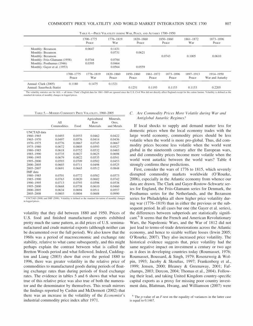
C. Are Commodity Prices More Volatile during War andAntiglobal Autarkic Regimes?

If local shocks to supply and demand matter less fordomestic prices when the local economy trades with thelarge world economy, commodity prices should be lessvolatile when the world is more pro-global. Thus, did com-modity prices become less volatile when the world wentglobal in the nineteenth century after the European wars,and did commodity prices become more volatile when theworld went autarkic between the world wars? Table 4strongly confirms these predictions.

First, consider the wars of 1776 to 1815, which severelydisrupted commodity markets worldwide (O’Rourke,2006), especially in the Atlantic economy from whence ourdata are drawn. The Clark and Gayer-Rostow-Schwartz ser-ies for England, the Friis-Glamann series for Denmark, thePosthumus series for the Netherlands, and the Bezansonseries for Philadelphia all show higher price volatility dur-ing war (1776–1819) than in either the previous or the sub-sequent period. In all cases bar one (the Gayer et al. series),the differences between subperiods are statistically signifi-cant.6 It seems that the French and American RevolutionaryWars, the Napoleonic Wars, and the War of 1812 did notjust lead to terms-of-trade deteriorations across the Atlanticeconomy, and hence to sizable welfare losses (Irwin 2005;O’Rourke, 2007). They also increased price volatility. Thehistorical evidence suggests that, price volatility had thesame negative impact on investment a century or two agoas it does in developing countries today (Roumasset, 1976;Roumasset, Boussard, & Singh, 1979; Rosenzweig & Wol-pin, 1993; Jacoby & Skoufias, 1997; Frankenberg et al.,1999; Jensen, 2000; Bleaney & Greenaway, 2001; Faf-champs, 2003; Dercon, 2004; Thomas et al., 2004). Follow-ing their lead, and taking United Kingdom country-specificcapital exports as a proxy for missing poor country invest-ment data, Blattman, Hwang, and Williamson (2007) were

TABLE 5.—MODERN COMMODITY PRICE VOLATILITY, 1960–2005

AllCommodities Food

AgriculturalRaw

Materials

Minerals,Ores,

and Metals

UNCTAD data1960–1965 0.0493 0.0553 0.0462 0.04221965–1970 0.0497 0.0576 0.0414 0.04361970–1975 0.0776 0.0867 0.0745 0.06671975–1980 0.0672 0.0805 0.0593 0.05271980–1985 0.0618 0.0752 0.0532 0.04831985–1990 0.0735 0.0827 0.0625 0.06981990–1995 0.0679 0.0822 0.0535 0.05411995–2000 0.0593 0.0709 0.0502 0.04532000–2005 0.0603 0.0711 0.0498 0.05252005–2007 0.0691 0.0665 0.0512 0.0848IMF data1980–1985 0.0701 0.0772 0.0582 0.05731985–1990 0.0763 0.0820 0.0602 0.07421990–1995 0.0713 0.0793 0.0598 0.05381995–2000 0.0668 0.0738 0.0610 0.04602000–2005 0.0634 0.0694 0.0511 0.05572005–2008 0.0803 0.0804 0.0608 0.0990

UNCTAD (2008) and IMF (2008). Volatility is defined as the standard deviation of monthly changesin logged prices.

TABLE 4.—PRICE VOLATILITY DURING WAR, PEACE, AND AUTARKY 1700–1950

1700–1775 1776–1819 1820–1860 1850–1860 1861–1872 1873–1896Peace War Peace Peace War Peace

Monthly: Bezanson 0.0647 0.1431Monthly: Bezanson 0.0731 0.0621Monthly: Bezanson 0.0743 0.1005 0.0610Monthly: Friis-Glamann (1958) 0.0744 0.0784Monthly: Posthumus (1946) 0.0395 0.0464Monthly: Gayer et al. (1953) 0.0564 0.0559

1700–1775 1776–1819 1820–1860 1850–1860 1861–1872 1873–1896 1897–1913 1914–1950Peace War Peace Peace Peace Peace Peace War and Autarky

Annual: Clark (2005) 0.1180 0.1475 0.1321Annual: Sauerbeck-Statist 0.1251 0.1193 0.1153 0.1153 0.2205

The volatility statistics are for ALL ¼ all items. Clark’s English data for 1861–1869 are ignored since the U.S. Civil War did not directly affect England except for the cotton famine. Volatility is defined as thestandard deviation of monthly changes in logged prices.

6 The p-value of an F-test on the equality of variances in the latter caseis equal to 0.1467.


able to show that for the period 1870 to 1940 a 1 standarddeviation increase in volatility was associated with a 33%to 58% decrease in capital inflows into poor countries. Dur-ing episodes of international conflict (and greater autarky),more price volatility would have reduced growth over andabove the negative effects that wartime investment crowd-ing out would have implied on its own (Williamson, 1984)and could thus help to explain the relatively slow growthexperienced during the British Industrial Revolution.

These data can also be used to explore the impact of theAmerican Civil War on commodity price volatility. Again,we know from the literature on the cotton famine that theCivil War had an impact on the terms of trade in cotton-importing and cotton-exporting parts of the world, but did itincrease commodity price volatility? In Britain, which wasnot a belligerent, the answer appears to be no, according tothe Sauerbeck-Statist evidence. Britain’s terms of trademay have deteriorated as a result of greater U.S. cottonscarcity, but it was still trading freely with the rest of theworld, and there was no increase in price volatility there.The United States underwent a quite different experience:the Bezanson price data show a very large (and statisticallysignificant) increase in volatility between 1861 and 1872 ascompared to what came before or after, a result consistentwith the fact that much of the American economy was cutoff from world markets during the conflict. The biggestantiglobal world regime in our period, however, was 1914to 1950, which saw two world wars and an intervening per-iod characterized by depression and autarky. During thefour decades 1914 to 1950, price volatility was twice asgreat as it was in the peacetime decades that preceded them,at least according to the Sauerbeck-Statist evidence. TheMintz quarterly price data, whose volatility is summarizedin table 6, certainly confirm this finding for the autarkicinterwar decades: the average volatility figure for all com-modities 1920 to 1950 is 0.039, or half again higher thanthe average for 1880 to 1914 and 1950 to 1963 (0.026).

This result mirrors that of Frederick Mills (1926) whoalmost a century ago found that two-thirds of the commod-ities whose prices he was investigating displayed greaterprice volatility during 1922 to 1925 than during 1906 to1913. His conclusion was that ‘‘the influence of the war-time disturbances upon individual prices has persisted,apparently, and, in so far as the four years from 1922 to1925 may be used as a criterion, has left us with more vari-able prices than we had during the years immediately pre-ceding the war’’ (p. 46).

As previously mentioned, Cuddington and Liang (2003)have explored the volatility of the price of commoditiesrelative to the price of manufactured goods. Using Grilliand Yang data (1988), they find that volatility was lowerbetween 1946 and 1971 than in any other subperiodbetween 1914 and 1938 (although volatility then increasedsubstantially after 1972).7 Cashin and McDermott (2002)find that the Economist’s annual industrial commodity priceindex from 1862 to 1999 documents a volatility increase inthe early 1900s (with World War I appearing to be animportant break point), and again after 1971. Unfortunatelythey do not present the data in such as way as to be able tosee clearly if the Bretton Woods period saw lower volatilitythan the 1914–1950 period. However, and as we have seen,the Mintz data in table 6 do confirm lower price volatilityduring the Bretton Woods era.

D. Robustness

Finally, we consider a more rigorous exercise that modelscommodity price changes as a GARCH(1,1) process.Beginning with the work of Engle (1982) and especiallyBollerslev (1986), the generalized autoregressive condi-

TABLE 6.—VOLATILITY OF U.S. EXPORT PRICES, 1880–1963

TotalFinished

ManufacturesSemimanufactures and

Crude Materials SemimanufacturesCrude

Materials Foods

1880–1885 0.0246 0.0277 0.0234 0.03411885–1890 0.0302 0.0167 0.0174 0.02541890–1895 0.0376 0.0254 0.0538 0.04051895–1900 0.0366 0.0322 0.0448 0.0471900–1905 0.0359 0.0181 0.0633 0.02261905–1910 0.0308 0.0117 0.0606 0.0271910–1914 0.0279 0.0128 0.0405 0.02831920–1925 0.0627 0.0428 0.0639 0.1184 0.09211925–1930 0.0295 0.0231 0.0349 0.0736 0.04251930–1935 0.0376 0.0505 0.0392 0.0612 0.04871935–1938 0.0264 0.0177 0.0494 0.0505 0.04591945–1950 0.039 0.0432 0.0395 0.0358 0.05151950–1955 0.0206 0.0164 0.0415 0.0366 0.03661955–1960 0.0082 0.0073 0.0347 0.0142 0.01371960–1963 0.0089 0.0074 0.0141 0.0176 0.00661950–1963 0.0125 0.0104 0.0225 0.0216 0.01771880–1950 0.0349 0.0263 0.0417

These volatility measures are based on the quarterly data reported in Mintz (1967, table A-3). Volatility is defined as the standard deviation of monthly changes in logged prices.

7 On the other hand, using the Boughton (1991) data, they find thatalthough 1946–1971 volatility was lower than 1927–1938 volatility, itwas higher than volatility between 1914 and 1926, and that volatility after1972 was higher still.


tional heteroskedastic (GARCH) framework has proved tobe an extremely robust approach to modeling the volatilityof time-series data. This success is mainly attributable to itsrecognition of the difference between unconditional andconditional variances and its incorporation of long memoryin the data-generating process and a flexible lag structure.In general, where et is the tth error term from an autoregres-sive model, the GARCH(p,q) specification assumes that theconditional variance equals

r2t ¼ E e2

t jXt

� �¼ aþ

Xp

i¼1

cie2t�iþ

Xq

j¼1

djr2t�j: ð1Þ

Thus, the conditional variance depends on its own pastvalues as well as lagged values of the residual term. Evenin a very parsimonious GARCH(1,1) specification, thetime-series behavior of changes in commodity prices is wellcaptured, as noted by Deb, Trivedi, and Varangis (1996),among others.

The use of GARCH also addresses the concern that byusing the standard deviation of period-over-period percen-tage changes in prices, we are in effect capturing ex postoutcomes rather than ex ante perceptions of commodityprice volatility. By now, it has become standard to treat theconditional variance recovered from estimating a GARCHprocess as just such an ex ante measure of commodity pricevolatility. Thus, the conditional variance should fully incor-porate any systematic changes in prices that might impartgreater volatility to commodities but are fully anticipated

by market participants, for example, any seasonality in agri-cultural prices.

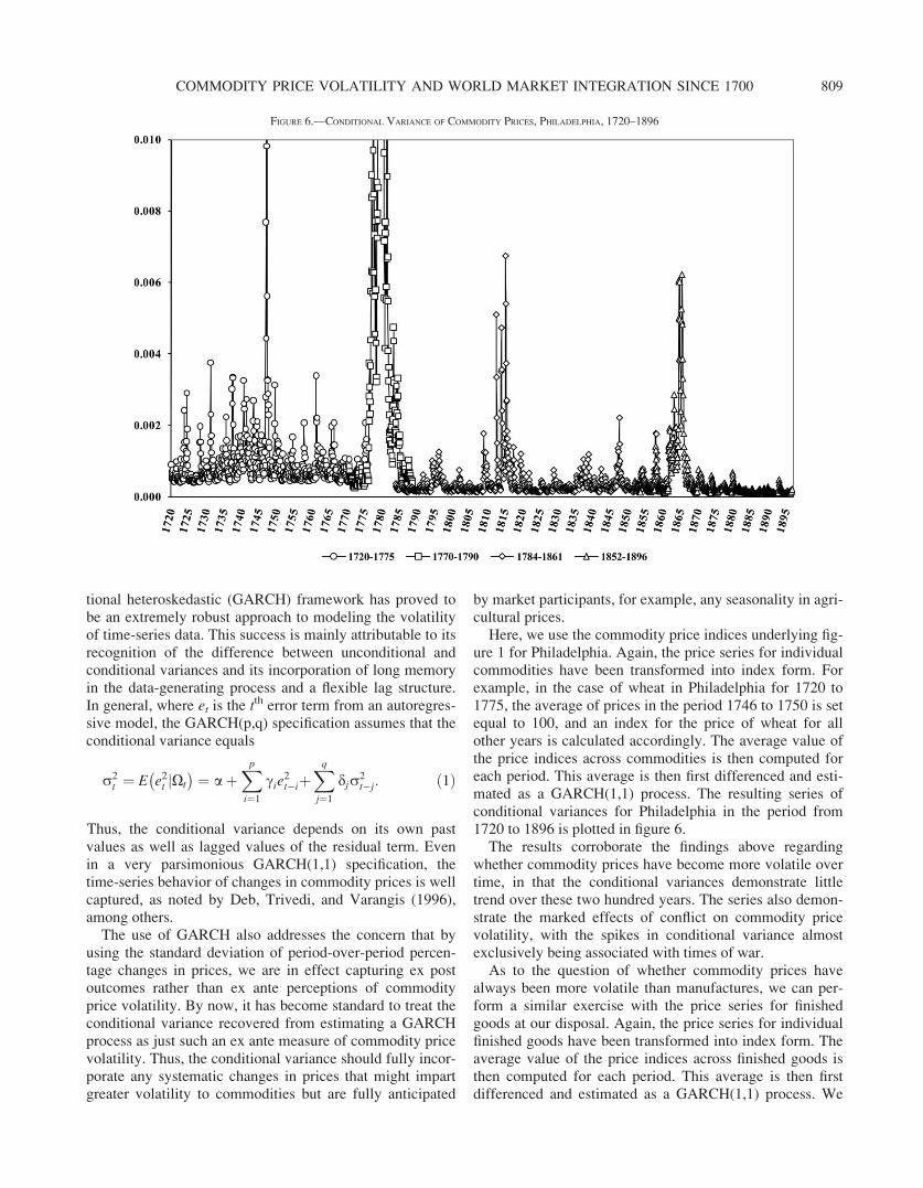
Here, we use the commodity price indices underlying fig-ure 1 for Philadelphia. Again, the price series for individualcommodities have been transformed into index form. Forexample, in the case of wheat in Philadelphia for 1720 to1775, the average of prices in the period 1746 to 1750 is setequal to 100, and an index for the price of wheat for allother years is calculated accordingly. The average value ofthe price indices across commodities is then computed foreach period. This average is then first differenced and esti-mated as a GARCH(1,1) process. The resulting series ofconditional variances for Philadelphia in the period from1720 to 1896 is plotted in figure 6.

The results corroborate the findings above regardingwhether commodity prices have become more volatile overtime, in that the conditional variances demonstrate littletrend over these two hundred years. The series also demon-strate the marked effects of conflict on commodity pricevolatility, with the spikes in conditional variance almostexclusively being associated with times of war.

As to the question of whether commodity prices havealways been more volatile than manufactures, we can per-form a similar exercise with the price series for finishedgoods at our disposal. Again, the price series for individualfinished goods have been transformed into index form. Theaverage value of the price indices across finished goods isthen computed for each period. This average is then firstdifferenced and estimated as a GARCH(1,1) process. We

FIGURE 6.—CONDITIONAL VARIANCE OF COMMODITY PRICES, PHILADELPHIA, 1720–1896


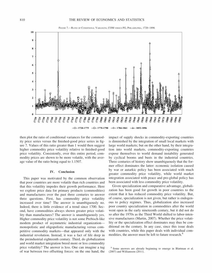
then plot the ratio of conditional variances for the commod-ity price series versus the finished-good price series in fig-ure 7. Values of this ratio greater than 1 would then suggesthigher commodity price volatility relative to finished-goodprice volatility. Consistently, over this entire period, com-modity prices are shown to be more volatile, with the aver-age value of the ratio being equal to 1.1507.

IV. Conclusion

This paper was motivated by the common observationthat poor countries are more volatile than rich countries andthat this volatility impedes their growth performance. Herewe explore price data for primary products (commodities)and manufactures over the past three centuries to answerthree questions. First, has commodity price volatilityincreased over time? The answer is unambiguously no.Indeed, there is little evidence of a trend since 1700. Sec-ond, have commodities always shown greater price volati-lity than manufactures? The answer is unambiguously yes.Higher commodity price volatility is not some Prebisch-likemodern product of asymmetric industrial organization—monopolistic and oligopolistic manufacturing versus com-petitive commodity markets—that appeared only with theindustrial revolution. Instead, it was a fact of life deep inthe preindustrial eighteenth century. Third, do globalizationand world market integration breed more or less commodityprice volatility? The answer is less. One can imagine a tugof war between two offsetting forces: on the one hand, the

impact of supply shocks in commodity-exporting countriesis diminished by the integration of small local markets withlarge world markets; but on the other hand, by their integra-tion into world markets, commodity-exporting countriesexpose themselves to world demand instability generatedby cyclical booms and busts in the industrial countries.Three centuries of history show unambiguously that the for-mer effect dominates the latter: economic isolation causedby war or autarkic policy has been associated with muchgreater commodity price volatility, while world marketintegration associated with peace and pro-global policy hasbeen associated with less commodity price volatility.

Given specialization and comparative advantage, globali-zation has been good for growth in poor countries to theextent that it has reduced commodity price volatility. But,of course, specialization is not given, but rather is endogen-ous to policy regimes. Thus, globalization also increasedpoor country specialization in commodities after the worldwent open in the early nineteenth century, but it did not doso after the 1970s as the Third World shifted to labor-inten-sive manufactures (Martin, 2007). Whether the price volati-lity or the specialization effect dominates may thus be con-ditional on the century. In any case, since this issue dealswith countries, while this paper deals with individual com-modities, the answer must be left to future research.8

FIGURE 7.—RATIO OF CONDITIONAL VARIANCES, COM VERSUS FG, PHILADELPHIA, 1720–1896

8 Some answers are already beginning to emerge in Blattman et al.(2007) and Williamson (2011).


REFERENCES

Acemoglu, Daron, Simon Johnson, James A. Robinson, and YunyongThaicharoen, ‘‘Institutional Causes, Macroeconomic Symptoms:Volatility, Crises, and Growth,’’ Journal of Monetary Economics50 (2003), 49–122.

Aghion, Philippe, George-Marios Angeletos, Abhijit Banerjee, and KalinaManova, ‘‘Volatility and Growth: Credit Constraints and Produc-tivity-Enhancing Investments,’’ NBER working paper no. 11349,(2005).

Aghion, Philippe, Philippe Bacchetta, Romain Ranciere, and KennethRogoff, ‘‘Exchange Rate Volatility and Productivity Growth: TheRole of Financial Development,’’ CEPR discussion paper no.5629, (2006).

Aizenman, Joshua, and Nancy Marion, ‘‘Volatility and Investment: Inter-preting Evidence from Developing Countries,’’ Economica 66(1999), 157–179.

Bezanson, Anne, Prices and Inflation during the American Revolution:Pennsylvania, 1770–1790 (Philadelphia: University of Pennsylva-nia Press, 1951).

Bezanson, Anne, Marjorie C. Denison, Miriam Hussey, and Elsa Kemp,Wholesale Prices in Philadelphia, 1852–1896 (Philadelphia: Uni-versity of Pennsylvania Press, 1954).

Bezanson, Anne, Robert D. Gray, and Miriam Hussey, Prices in ColonialPennsylvania (Philadelphia: University of Pennsylvania Press,1935).

——— Wholesale Prices in Philadelphia, 1784–1861 (Philadelphia: Uni-versity of Pennsylvania Press, 1936).

Blattman, Christopher, Jason Hwang, and Jeffrey G. Williamson, ‘‘TheImpact of the Terms of Trade on Economic Development in thePeriphery, 1870–1939: Volatility and Secular Change,’’ Journal ofDevelopment Economics 82 (2007), 156–179.

Bleaney, Michael, and David Greenaway, ‘‘The Impact of Terms of Tradeand Real Exchange Rate Volatility on Investment and Growth inSub-Saharan Africa,’’ Journal of Development Economics 65(2001), 491–500.

Bollerslev, Tim, ‘‘Generalized Autoregressive Conditional Heteroskedas-ticity,’’ Journal of Econometrics 31 (1986), 307–327.

Boughton, James M, ‘‘Commodity and Manufactures Prices in the LongRun,’’ IMF working paper no. WP/91/47 (1991).

Cashin, Paul, and C. John McDermott, ‘‘The Long-Run Behavior of Com-modity Prices: Small Trends and Big Variability,’’ IMF staffpapers 49 (2002), 175–199.

Clark, Gregory, ‘‘The Condition of the Working Class in England, 1209–2004,’’ Journal of Political Economy 113 (2005), 1307–1340.

Cuddington, John T., and Hong Liang, ‘‘Commodity Price Volatilityacross Exchange Rate Regimes,’’ Georgetown University and IMFmimeograph (2003).

Cuddington, John T., Rodney Ludema, and Shamila A. Jayasuriya, ‘‘Pre-bisch-Singer Redux,’’ in D. Lederman and W. F. Maloney (Eds.),Natural Resources: Neither Curse nor Destiny (Stanford: StanfordUniversity Press, 2007).

Davenant, Charles, An Essay upon the Probable Methods of Making Peo-ple Gainers in the Balance of Trade (London: James Knapton,1699).

Deaton, Angus S., ‘‘Commodity Prices and Growth in Africa,’’ Journal ofEconomic Perspectives 13 (1999), 23–40.

Deaton, Angus S., and Ronald I. Miller, ‘‘International CommodityPrices, Macroeconomic Performance and Politics in Sub-SaharanAfrica,’’ Journal of African Economics 5 (1996), 99–191.

Deb, Partha, Pravin K. Trivedi, and Panayotis Varangis, ‘‘The Excess Co-movement of Commodity Prices Reconsidered,’’ Journal ofApplied Econometrics 11 (1996), 275–291.

Dercon, Stefan, Insurance against Poverty (New York: Oxford UniversityPress, 2004).

Elbers, Chris, Jan Willem Gunning, and Bill Kinsey, ‘‘Growth and Risk:Methodology and Micro Evidence,’’ World Bank EconomicReview 21:1 (2007), 1–20.

Engle, Robert F., ‘‘Autoregressive Conditional Heteroskedasticity withEstimates of the Variance of United Kingdom Inflation,’’ Econo-metrica 50 (1982), 987–1008.

Fafchamps, Marcel, Rural Poverty, Risk and Development (Cheltenham:Edward Elgar, 2003).

Fatas, Antonio, and Ilian Mivhov, ‘‘Policy Volatility, Institutions andEconomic Growth,’’ INSEAD, unpublished manuscript.

Flug, Karnit, Antonio Spilimbergo, and Erik Wachtenheim, ‘‘Investmentin Education: Do Economic Volatility and Credit Constraints Mat-ter?’’ Journal of Development Economics 55 (1999), 465–481.

Frankenberg, Elizabeth, Kathleen Beegle, Bondan Sikoki, and DuncanThomas, ‘‘Health, Family Planning and Well-Being in Indonesiaduring an Economic Crisis: Early Results from the IndonesianFamily Life Survey,’’ RAND Labor and Population Program work-ing paper series 99-06 (1999).

Friis, Astrid, and Kristof Glamann, A History of Prices and Wages inDenmark, 1660–1800 (London: Longmans Green, 1958).

Gayer, Arthur D., Walt W. Rostow, and Anna J. Schwartz, Microfilmedto The Growth and Fluctuation of the British Economy, 1790–1850 (Oxford: Clarendon Press, 1953).

Grilli, Enzo, and Maw Cheng Yang, ‘‘Primary Commodity Prices, Manu-factured Goods Prices, and the Terms of Trade of DevelopingCountries: What the Long Run Shows,’’ World Bank EconomicReview 2 (1988), 1–47.

Hnatkovska, Viktoria, and Norman Loayza, ‘‘Volatility and Growth,’’ inJ. Aizenman and B. Pinto (Eds.), Managing Economic Volatilityand Crises: A Practitioner’s Guide (Cambridge: Cambridge Uni-versity Press, 2005).

International Monetary Fund, Primary Commodity Prices Database(2008).

Irwin, Douglas A., ‘‘The Welfare Cost of Autarky: Evidence from the Jef-fersonian Trade Embargo, 1807–09,’’ Review of International Eco-nomics 13 (2005), 631–645.

Jacoby, Hana G., and Emmanuel Skoufias, ‘‘Risk, Financial Markets, andHuman Capital in a Developing Country,’’ Review of EconomicStudies 64 (1997), 311–335.

Jensen, Robert, ‘‘Agricultural Volatility and Investments in Children,’’American Economic Review 90 (2000), 399–404.

Koren, Miklos, and Silvana Tenreyro, ‘‘Volatility and Development,’’Quarterly Journal of Economics 122 (2007), 243–287.

Lewis, W. Arthur, The Evolution of the International Economic Order(Princeton, N.J.: Princeton University Press, 1978).

Loayza, Norman V., Romain Ranciere, Luis Serven, and Jaume Ventura,‘‘Macroeconomic Volatility and Welfare in Developing Countries:An Introduction,’’ World Bank Economic Review 21 (2007), 343–357.

Martin, Will, ‘‘Outgrowing Resource Dependence: Theory and Develop-ments,’’ in D. Lederman and W. F. Maloney (Eds.), NaturalResources: Neither Curse nor Destiny (Stanford: Stanford Univer-sity Press, 2007).

Mills, Frederick C., The Behavior of Prices (New York: National Bureauof Economic Research, 1926).

Mintz, Ilse, Cyclical Fluctuations in the Exports of the United States since1879 (New York: National Bureau of Economic Research, 1967).

O’Rourke, Kevin H., ‘‘The Worldwide Economic Impact of the FrenchRevolutionary and Napoleonic Wars, 1793–1815,’’ Journal of Glo-bal History 1 (2006), 123–149.

——— ‘‘War and Welfare: Britain, France and the United States, 1807–14,’’ Oxford Economic Papers, no. 59 (2007), i8–i30.

O’Rourke, Kevin H., and Jeffrey G. Williamson, ‘‘When Did Globaliza-tion Begin?’’ European Review of Economic History 6 (2002), 23–50.

Persson, Karl Gunnar, Grain Markets in Europe, 1500–1900 (Cambridge:Cambridge University Press, 1999).

Poelhekke, Steven, and Frederick van der Ploeg, ‘‘Volatility, FinancialDevelopment and the Natural Resource Curse,’’ CEPR discussionpaper no. 6513 (2007).

Posthumus, Nicolaas W., Inquiry into the History of Prices in Holland(Leiden: Brill, 1946).

Prebisch, Raul, ‘‘The Economic Development of Latin America and ItsPrincipal Problems,’’ Economic Bulletin for Latin America 7(1950), 1–22.

Radetzki, Marian, A Handbook of Primary Commodities in the GlobalEconomy (Cambridge: Cambridge University Press, 2008).

Ramey, Garey, and Valerie A. Ramey, ‘‘Cross-Country Evidence on theLink between Volatility and Growth,’’ American Economic Review85 (1995), 1138–1151.

Roumasset, James A., Rice and Risk: Decision-Making among Low-Income Farmers (Amsterdam: North-Holland, 1976).

Roumasset, James A., Jean-Marc Boussard, and Inderjit Singh (Eds.),Risk, Uncertainty and Agricultural Development (New York: Agri-cultural Development Council, 1979).


Rosenzweig, Mark R., and Kenneth I. Wolpin, ‘‘Credit Market Con-straints, Consumption Smoothing, and the Accumulation of Dur-able Production Assets in Low Income Countries: Investments inBullocks in India,’’ Journal of Political Economy 101 (1993),223–244.

Sauerbeck, Augustus, ‘‘Prices of Commodities and the Precious Metals,’’Journal of the Statistical Society of London 49 (1886), 581–648.

——— ‘‘Prices of Commodities during the Last Seven Years,’’ Journalof the Royal Statistical Society 56 (1893), 215–254.

——— ‘‘Prices of Commodities in 1908,’’ Journal of the Royal StatisticalSociety 72 (1908), 68–80.

——— ‘‘Wholesale Prices of Commodities in 1916,’’ Journal of theRoyal Statistical Society 80 (1917), 289–309.

Statist, ‘‘Wholesale Prices of Commodities in 1929,’’ Journal of the RoyalStatistical Society 93 (1930), 271–287.

——— ‘‘Wholesale Prices in 1950,’’ Journal of the Royal StatisticalSociety 114 (1951), 408–422.

Szirmai, Adam, The Dynamics of Socio-Economic Development: AnIntroduction (Cambridge: Cambridge University Press, 2005).

Thomas, Duncan, Kathleen Beegle, Elizabeth Frankenberg, BondanSikoki, John Strauss, and Graciela Teruel, ‘‘Education in a Crisis,’’Journal of Development Economics 74 (2004), 53–85.

UNCTAD, Commodity Price Statistics (New York: U.N. Conference onTrade and Development, 2007).

——— Trade and Development Report, 2008 (New York: U.N. Confer-ence on Trade and Development, 2008).

Williamson, Jeffrey G., ‘‘Why Was British Growth So Slow during theIndustrial Revolution?’’ Journal of Economic History 44 (1984),687–712.

——— ‘‘Globalization and the Great Divergence: Terms of Trade Boomsand Volatility in the Poor Periphery, 1782–1913,’’ EuropeanReview of Economic History 12 (2008), 355–391.

——— Trade and Poverty: When the Third World Fell Behind (Cam-bridge, MA: MIT Press, 2011).

APPENDIX A

Commodity Classifications for Historical Price Data

Philadelphia, 1720–1775

AF: Beef; Bread, middling; Corn; Flour; Molasses; Pork; Rice; Salt,coarse; Salt, fine; Sugar, Muscavado; Wheat

ARM: Pitch; Staves, hogshead; Staves, pipe; TarFG: Rum, West Indian; Turpentine; Wine, Madeira


AF: Beef; Bread, ship; Chocolate; Coffee; Flour, common; Flour, mid-dling; Flour, superior; Molasses; Pepper; Pork; Rice; Sugar, loaf;Sugar, Muscavado; Tea, Bohea; Wheat

ARM: Cotton; Indigo; Leather, sole; Tar; TobaccoFG: Iron, bar; Rum, West Indian; Turpentine; Wine


AF: Almonds; Beef; Beef, mess; Bread; Bread, pilot; Butter; Cheese;Chocolate; Clove; Cocoa; Codfish, dried; Coffee; Corn; Corn meal;Currents; Flaxseed; Flour, superfine; Ginseng; Hams; Herring;Honey; Lard; Lemons; Mace; Mackerel; Mackerel 1; Mackerel 3;Molasses; Nutmeg; Oats; Peas; Pepper; Pimento; Pork; Pork, Bur-lington & mess; Pork, prime; Raisins; Rice; Rye; Rye meal; Salt,coarse; Salt, fine; Sugar, Havana brown; Sugar, Havana white;Sugar, loaf and lump; Tea; Tea, Hyson; Tea, Souchong; Wheat

ARM: Beaver; Beeswax, yellow; Cotton; Deer skins; Feathers; Flax;Fustic; Hemp, Russian; Hides; Indigo; Leather; Logwood; Log-wood, Campeachy; Muskrat; Oil, linseed; Oil, sweet; Oil, sperm;Oil, whale; Pine, heart and panel; Pine, sap; Pitch; Rosin; Spirits ofturpentine; Starch; Staves, barrel; Staves, hogshead; Staves, pipe;Tallow; Tar; Tobacco, James River; Tobacco, Kentucky

MOM: Alum; Ashes, pearl; Ashes, pot; Brimstone, rolls; Coal, Virgi-nia; Copper, sheathing; Lead; Lead, red dry; Lead, white dry; Lead,white in oil; Saltpeter, refined; Verdigris

FG: Brandy, French; Candles, sperm; Candles, tallow; Candles, tallowtipped; Candles, tallow mold; Copperas; Cordage, foreign; Duck,bear ravens; Gin, Holland; Ginger, ground; Gunpowder; Iron, bardomestic; Iron, bar foreign; Iron, bar Swedish; Iron, pig; Iron, sheet;Nails; Plaster of Paris; Rum, New England; Sheeting, Russianbrown; Shingles; Shot; Soap, Castile; Soap, white; Soap, yellow;Spanish Brown, dry; Spanish Brown, in oil; Steel, American; Steel,English; Steel, German; Steel, T Crowley; Tin, plate; Turpentine;Wine, Lisbon; Wine, Madeira; Wine, Malaga; Wine, port; Wine,sherry; Wine, Tenerife cargo


AF: Almonds; Beef, dried; Beef, hams; Beef, mess; Butter; Cheese;Cloves; Cocoa; Codfish, dried; Coffee; Corn; Corn meal; Currants;Flour, Superfine; Ginger, race; Hams; Herring; Lard; Lemons;Mace; Mackerel; Molasses; Nutmeg; Oats; Pepper; Pimento; Pork,Burlington and mess; Raisins; Rice; Rye; Salt, coarse; Salt, fine;Sugar, loaf and lump; Tea; Tea, Hyson; Tea, Souchong; Wheat, redPennsylvania

ARM: Beaver; Beeswax, yellow; Cotton, LA & MS; Deer skins;Feathers; Fustic; Hemp, Russian; Hides; Indigo; Leather; Logwood;Logwood, Campeachy; Muskrat; Oil, linseed; Oil, sperm; Oil,whale; Pine, heart and panel; Pitch; Rosin; Starch; Staves, barrel;Staves, hogshead; Staves, pipe; Tallow; Tar

MOM: Alum; Ashes, pearl; Ashes, pot; Brimstone, rolls; Coal, bitumi-nous; Copper, sheathing; Lead, bar; Lead, red dry; Lead, white dry;Lead, white in oil; Saltpeter, refined; Verdigris

FG: Candles, adamantine; Candles, sperm; Copperas; Cordage, for-eign; Gin, Holland; Gunpowder; Iron, bar domestic; Iron, pig; Iron,sheet; Nails; Plaster of Paris; Rum, New England; Sheeting, Russianbrown; Shingles; Shot; Soap, Castile; Spirits of turpentine; Steel,American; Steel, English; Steel, German; Tin, plate; Wine, Madeira;Wine, Malaga; Wine, port; Wine, sherry

Britain, 1790–1850

AF: Beef; Butter; Cinnamon; Cocoa; Coffee; Ginger; Liqourice; Oats;Pepper; Pork; Seeds; Sugar; Tea; Wheat

ARM: Annato; Balsam; Barilla; Beeswax; Bristles; Camphor; Cochi-neal; Cotton; Flax; Fustic; Hemp; Hides; Indigo; Isinglass; Leatherbutts; Linseed; Linseed oil; Logwood; Madder root; Mahogany;Olive oil; Quinine; Rape oil; Raw silk; Starch; Staves; Sumac; Tal-low; Tar; Timber; Tobacco; Whale fins; Whale oil; Wool

MOM: Alum; Ashes; Brimstone; Copper; Lead; Quicksilver; SalAmmoniac; Saltpetre; Vitriol

FG: Brandy; Iron; Iron, bars; Iron, pig; Rum; Silk, thrown; Soap,mottled; Soap, yellow; Tin, black; Turpentine; Wine

Denmark, 1750–1800

AF: Bacon; Barley; Barley groats; Buckwheat groats; Butter, Funen;Cheese, Holstein; Cod, Icelandic salted; Cod, split; Herring, Danishautumn; Malt; Oatmeal; Oats; Peas; Rye, Danish; Salt, Copenhagen;Salt, Spanish; Stockfish, Icelandic; Wheat, Danish

ARM: Beechwood, Holstein; Flax; Hemp; Hops, Brunswick; Tallow;Tar; Train oil

FG: Brandy, French; Iron, Norwegian; Soap, soft; Wine, French

The Netherlands, 1750–1800

AF: Barley, Frisian winter; Beans, horse; Buckwheat, Brabant; Candy,white; Cinnamon; Cloves; Cocoa, Caracas; Nutmeg; Oats, forage;Rye, Konigsberg; Salt, white; Stockfish, split; Sugar, loaf; Sugar,refined; Sugar, Surinam; Tea, Buoy; Treacle; Wheat, Polish

ARM: Camphor, refined; Codliver oil; Coleseed, Flemish; Cotton,Smyrna; Hides, native, salted; Indigo, Java; Linseed, Riga, crushed;Linseed oil; Madder, common; Opium; Rape oil; Sole leather;


Starch; Tobacco; Train, oil; Whale bones; Wool, Andalusian; Wool,Segovia, washed

MOM: Alum, English; Borax, refined; Lead, white; Potash, Dantzig;Sulphur, refined

FG: Copperas, English; Gunpowder; Iron, single, white; Sail yarn;Soap, Marseilles; Thread, card, Maastricht; Turpentine, Venetian;Wine, Bordeaux

England, 1700–1869

AF: Barley; Beans; Beef; Beer, strong; Butter; Cheese; Eggs; Flour;Milk; Mutton; Oats; Peas; Pork; Raisins; Rice; Salt; Sugar; Wheat;Wheat flour

ARM: Firewood; Hay; Hops; Lamp oil; Suet; Wood; WoolMOM: Coal; Coal, London; Coal, rest of EnglandFG: Candles, tallow; Cloth, wool; Clothing; Iron manufactureds;

Paper, foolscap; Shoes; Soap

Britain, 1850–1950

AF: Bacon; Barley; Beef, middling; Beef, prime; Butter; Coffee, Cey-lon; Coffee, Rio; Flour; Maize; Mutton, middling; Mutton, prime;Oats; Pork; Potatoes; Rice; Sugar, Java; Tea; Wheat, English

ARM: Cotton; Cotton, Dollegargh; Flax, Russian; Hemp, Manila;Hemp, Russian; Hides, Argentine; Indigo; Jute; Leather; Linseedoil; Olive oil; Palm oil; Seeds; Silk; Timber, hewn; Wool, Adelaide;Wool, English; Wool, Merino

MOM: Coals, Export; Coals, Wallsend; Copper, Chile; Lead; Nitrate

APPENDIX B

Commodity Classifications for Modern Price Data

IMF, 1980–2008

AF: Bananas, Central American and Ecuador; Barley, Canadian no.1western; Beef, Australian and New Zealand lean fores; Cocoabeans; Coffee, other mild arabicas; Coffee, robusta; Fish, farm bred

Norwegian salmon; Groundnuts; Lamb, frozen carcass SmithfieldLondon; Maize, U.S. No. 2 yellow; Olive oil, extra virgin; Oranges;Palm oil; Poultry, whole chicken; Rapeseed oil, Crude; Rice, milledwhite; Shrimp, frozen shell-on headless; Soybean meal; Soybeanoil, exchange approved grades; Soybeans, United States No. 2 yel-low and par; Sugar, European import price; Sugar, Free Market;Sugar, U.S. import price; Sunflower oil; Swine, hogs; Tea, Mom-basa; Wheat, No.1 hard red winter

ARM: Cotton, middling; Fishmeal, Peru fish meal/pellets; Hides,heavy native steers; Logs, hard, best quality Malaysian meranti;Logs, soft, Douglas fir; Rubber, no.1 rubber smoked sheet; Sawn-wood, hard, dark red meranti; Sawnwood, soft, Douglas fir; Wool,coarse; Wool, fine

MOM: Coal, Australian thermal; Copper, grade A cathode; Iron ore,fine; Lead; Nickel, melting grade; Tin, standard grade; Uranium,u3o8; Zinc, high grade

UNCTAD, 1960–2007

AF: Bananas, Central America and Ecuador; Beef, Australia and NewZealand, frozen boneless; Cocoa beans; Coconut oil, Philippines;Coffee, Brazilian and other natural arabicas; Coffee, Colombian mildarabicas; Coffee, other mild arabicas; Coffee, robustas; Copra, Philip-pines/Indonesia; Cottonseed oil, United States; Fish meal; Groundnutoil; Palm kernel oil, Malaysia; Palm oil, mainly Indonesian; Pepper,white Sarawak/Muntok; Rice, Thailand, white milled; Soybean meal;Soybean oil; Soybeans, United States, No. 2 yellow; Sugar, in bulk;Sunflower oil; Wheat, United States, No. 2 hard red winter

ARM: Cattle hides, United States, Chicago packer’s heavy nativesteers; Cotton, Egypt, Giza 88, good; Cotton, Pakistan Sind/Punjab,SG Afzal; Cotton, United States, Memphis/Eastern, Middling; Cot-ton, United States, Memphis/Orleans/Texas, Middling; Jute, Bangla-desh, BWD; Linseed oil; Rubber, in bales, No. 1 RSS; Sisal, Tanza-nia/Kenya, No. 2 and 3 long; Sisal, Tanzania/Kenya, No. 3 and UG;Tobacco, unmanufactured

MOM: Aluminum, high grade; Copper, grade A, electrolytic wire bars/cathodes; Copper, wire bars; Iron ore, Brazilian; Lead; Manganeseore; Nickel cathodes; Phosphate rock, Khouribga; Tin; Tungstenore; Zinc, Prime Western; Zinc, special high grade


Documents

Commodity Price Volatility and World Market Integration