International Journal of Computer Applications (0975 – 8887)

Volume 85 – No 7, January 2014

12

Bank Direct Marketing Analysis of Data Mining

Techniques

Hany A. Elsalamony Mathematics Department, Faculty of Science, Helwan University, Cairo, Egypt

Computer Science & Information Department, Arts & Science College, Salman University, Saudi Arabia

ABSTRACT

All bank marketing campaigns are dependent on customers’

huge electronic data. The size of these data sources is

impossible for a human analyst to come up with interesting

information that will help in the decision-making process.

Data mining models are completely helping in the

performance of these campaigns. This paper introduces

analysis and applications of the most important techniques in

data mining; multilayer perception neural network (MLPNN),

tree augmented Naïve Bayes (TAN) known as Bayesian

networks, Nominal regression or logistic regression (LR), and

Ross Quinlan new decision tree model (C5.0). The objective

is to examine the performance of MLPNN, TAN, LR and

C5.0 techniques on a real-world data of bank deposit

subscription. The purpose is increasing the campaign

effectiveness by identifying the main characteristics that

affect a success (the deposit subscribed by the client) based on

MLPNN, TAN, LR and C5.0. The experimental results

demonstrate, with higher accuracies, the success of these

models in predicting the best campaign contact with the

clients for subscribing deposit. The performances are

calculated by three statistical measures; classification

accuracy, sensitivity, and specificity.

General Terms

Bank Marketing; Data Mining Techniques.

Keywords

Bank Marketing; Naïve Bayes; Nominal Regression; Neural

Network; C5.0.

1. INTRODUCTION In banks, huge data records information about their customers.

This data can be used to create and keep clear relationship and

connection with the customers in order to target them

individually for definite products or banking offers. Usually,

the selected customers are contacted directly through:

personal contact, telephone cellular, mail, and email or any

other contacts to advertise the new product/service or give an

offer, this kind of marketing is called direct marketing. In fact,

direct marketing is in the main a strategy of many of the banks

and insurance companies for interacting with their customers

[19].

Historically, the name and identification of the term direct

marketing suggested first time in 1967 by Lester Wunderman,

which he is considered to be the father of direct marketing

[11].

In addition, some of the banks and financial-services

companies may depend only on strategy of mass marketing

for promoting a new service or product to their customers. In

this strategy, a single communication message is broadcasted

to all customers through media such as television, radio or

advertising firm, etc. [18]. In this approach, companies do not

set up a direct relationship to their customers for new-product

offers. In fact, many of the customers are not interesting or

respond to this kind of sales promotion [20].

Accordingly, banks, financial-services companies and other

companies are shifting away from mass marketing strategy

because its ineffectiveness, and they are now targeting most of

their customers by direct marketing for specific product and

service offers [19, 20]. Due to the positive results clearly

measured; many marketers attractive to the direct marketing.

For example, if a marketer sends out 1,000 offers by mail and

100 respond to the promotion, the marketer can say with

confidence that the campaign led immediately to 10% direct

responses. This metric is known as the 'Response Rate', and it

is one of many clear quantifiable success metrics employed by

direct marketers. In dissimilarity, general advertising uses

indirect measurements, such as awareness or engagement,

since there is no direct response from a consumer [11]. From

the literature, the direct marketing is becoming a very

important application in data mining these days. The data

mining has been used widely in direct marketing to identify

prospective customers for new products, by using purchasing

data, a predictive model to measure that a customer is going to

respond to the promotion or an offer [7].

Data mining has gained popularity for illustrative and

predictive applications in banking processes. Four techniques

will apply to the data set on the bank direct marketing. The

Multilayer perception neural network (MLPNN) is one of

these techniques, which have their roots in the artificial

intelligence. MLPNN is a mutually dependent group of

artificial neurons that applying a mathematical or

computational model for information processing using a

connected approach to computation (Freeman et al., 1991)

[13, 24, 27].

Another technique of data mining is the decision tree

approach. Decision tree provides powerful techniques for

classification and prediction. There are many algorithms to

build a decision tree model [9, 16]. It can generate

understandable rules, and to handle both continuous and

categorical variables [23]. One of the famous recent

techniques of the decision tree is C5.0, which will be applied

in this paper.

A naïve Bayes classifier (TAN) is an easy and simple

probabilistic classifier based on applying Bayes' theorem with

strong (naïve) independence assumptions. It can predict class

membership probabilities, such as the probability that a given

sample belongs to a particular class. The assumption is called

class conditional independence. It is made to simplify the

computation involved and, in this sense, is considered “naïve”

[16].

The fourth technique will be using is Logistic regression

analysis (LR). Cornfield was the first to use logistic regression

in the early 1960s and with the wide availability of

sophisticated statistical software for high-speed computers;

the use of logistic regression is increasing. LR studies the

International Journal of Computer Applications (0975 – 8887)

Volume 85 – No 7, January 2014

13

association between a categorical dependent and a set of

independent (descriptive) fields. The name logistic

regression is often used when the dependent variable has only

two values. The name multiple-group logistic regression

(MGLR) is usually reserved for the case when the dependent

variable has three or more unique values. Multiple-group

logistic regression is sometimes called multinomial,

polytomous, polychotomous, or nominal logistic regression

[4].

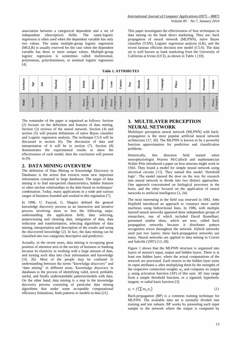
This paper investigates the effectiveness of four techniques in

data mining on the bank direct marketing. They are: back

propagation of neural network (MLPNN), naïve Bayes

classifier (TAN), Logistic regression analysis (LR), and the

recent famous efficient decision tree model (C5.0). The data

set is well known as bank marketing from the University of

California at Irvine (UCI), as shown in Table 1 [10].

Table 1. ATTRIBUTES

Att

rib

ute

s

Age

Job

Marit

al

Ed

ucati

on

Defu

lt

Bala

nce

Hou

sin

g

Loan

Con

tact

Day

Mon

th

Du

rati

on

Cam

pagn

Pd

ays

Previo

us

Pou

tcom

e

Ou

tpu

t

Kin

d

Num

eric

Cat

egori

cal

Cat

egori

cal

Cat

egori

cal

Bin

ary

(Cat

egori

ca

l)

Num

eric

Bin

ary

(Cat

egori

ca

l)

Bin

ary

(Cat

egori

ca

l)

Cat

egori

cal

Num

eric

Cat

egori

cal

Num

eric

Num

eric

Num

eric

Num

eric

Cat

egori

cal

Bin

ary

(Cat

egori

ca

l)

The remainder of the paper is organized as follows: Section

(2) focuses on the definition and features of data mining.

Section (3) reviews of the neural network. Section (4) and

section (5) will present definitions of naïve Bayes classifier

and Logistic regression analysis. The technique C5.0 will be

discussed in section (6). The discussion of data and

interpretation of it will be in section (7). Section (8)

demonstrates the experimental results to show the

effectiveness of each model, then the conclusion will present

in (9).

2. DATA MINING OVERVIEW The definition of Data Mining or Knowledge Discovery in

Databases is the action that extracts some new important

information contained in large databases. The target of data

mining is to find unexpected characteristics, hidden features

or other unclear relationships in the data based on techniques’

combination. Today, many applications in a wide and various

ranges of business founded and worked in this regulation [7].

In 1996, U. Fayyad, G. Shapiro defined the general

knowledge discovery process as an interactive and iterative

process involving more or less the following steps:

understanding the application field, data selecting,

preprocessing and cleaning data, integration of data, data

reduction and transformation, selecting algorithms of data

mining, interpretation and description of the results and using

the discovered knowledge [2]. In fact, the data mining can be

classified into two categories descriptive and predictive.

Actually, in the recent years, data mining is occupying great

position of attention area in the society of business or banking

because its elasticity in working with a large amount of data,

and turning such data into clear information and knowledge

[16, 26]. Most of the people may be confused in

understanding between the terms “knowledge discovery” and

“data mining” in different areas. Knowledge discovery in

databases is the process of identifying valid, novel, probably

useful, and finally understandable patterns/models with data.

On the other hand, data mining is a step in the knowledge

discovery process consisting of particular data mining

algorithms that under some acceptable computational

efficiency limitations, finds patterns or models in data [21].

3. MULTILAYER PERCEPTION

NEURAL NETWORK Multilayer perception neural network (MLPNN) with back-

propagation is the most popular artificial neural network

architecture [17, 26]. The MLPNN is known to be a powerful

function approximation for prediction and classification

problems.

Historically, this direction field started when

neurophysiologist Warren McCulloch and mathematician

Walter Pitts introduced a paper on how neurons might work in

1943. They found a model for simple neural network using

electrical circuits [13]. They named this model ‘threshold

logic’. The model opened the door on the way for research

into neural network to divide into two distinct approaches.

One approach concentrated on biological processes in the

brain, and the other focused on the application of neural

networks to artificial intelligence [3, 24].

The most interesting in the field was renewed in 1982. John

Hopfield introduced an approach to construct more useful

machines using bidirectional lines. In 1986, with multiple

layered neural networks appeared three independent groups of

researchers, one of which included David Rumelhart,

presented similar ideas, which are now, called back

propagation networks because it distributes pattern

recognition errors throughout the network. Hybrid networks

used just two layers; these back-propagation networks use

many. Neural networks are applied to data mining in Craven

and Sahvlik (1997) [13, 28].

Figure 1 shows that the MLPNN structure is organized into

layers of neuron's input, output and hidden layers. There is at

least one hidden layer, where the actual computations of the

network are processed. Each neuron in the hidden layer sums

its input attributes xi after multiplying them by the strengths of

the respective connection weights wij and computes its output

yj using activation function (AF) of this sum. AF may range

from a simple threshold function, or a sigmoid, hyperbolic

tangent, or radial basis function [3].

(1)

Back-propagation (BP) is a common training technique for

MLPNN. The available data set is normally divided into

training and test subsets. BP works by presenting each input

sample to the network where the output is computed by

International Journal of Computer Applications (0975 – 8887)

Volume 85 – No 7, January 2014

14

performing weighted sums and transfer functions. The sum of

squared differences between the desired and asset value of the

output neuron's E is defined as:

(2)

Where ydj is the desired value of an output neuron j, and yj is

the output of that neuron.

Fig 1. The structure of multilayer perceptron neural

network.

Weights wij in Equation (1), are adjusted to finding the

minimum error E of Equation (2) as fast, quickly as possible.

BP applies a weight correction to reduce the difference

between the network outputs and the desired ones; i.e., the

neural network can learn, and can thus reduce the future

errors. The performance of MLPNN depends on network

parameters, the network weights and the type of transfer

functions used [25].

When using MLPNN, three important issues need to be

addressed; the selection of data samples for network training,

the selection of an appropriate and efficient training algorithm

and determination of network size. New algorithms for data

portioning and effective training with faster convergence

properties and fewer computational requirements are being

developed [26]. However, the third issue is a more difficult

problem to solve. It is necessary to find a network structure

small enough to meet certain performance specifications.

Pruning methods for improving the input-side redundant

connections were also developed that resulted in smaller

networks without degrading or compromising their

performance [17].

Finally, MLPNN has many advantages, such as the good

learning ability, less memory demand, suitable generalization,

fast real-time operating, simple and convenient to utilize,

suited to analyze complex patterns, and so on. Therefore, it

has become a research hotspot in the past few years. On the

other hand, there are some disadvantages like: the neural

network requires high-quality data; variables must be

carefully selected a priori, the risk of over-fitting, and requires

a definition of architecture [13].

4. NAÏVE BAYES CLASSIFIER Naïve Bayes (TAN) is one of the most effective and efficient

classification algorithms. It is a one special case of a Bayesian

network. The structure and parameters of the unconstrained

Bayesian network would appear to be a logical means of

improvement. However, (TAN) was found by Friedman

(1997) as an easily outperforms such an unconstrained

Bayesian network classifier on a huge sample of benchmark

data sets. Bayesian classifiers are helpful in predicting the

probability that a sample belongs to a particular class or

grouping. This technique is useful for large databases because

it is highly accurate and quickly in classification and fast to

train with simple models and intuitive. It requires a small

amount of training data to estimate the parameters (means and

variances of the variables) necessary for classification,

handles real and discrete data, also it can handle streaming

data well. In another way, some often apparent disadvantages

of Bayesian analysis are really not problems in practice. Any

ambiguities in a prior choosing are generally not dangerous,

since the various possible convenient priors usually do not

disagree strongly within the regions of interest. Bayesian

analysis is not limited to what is traditionally considered

statistical data, but can be applied to any space of models

[12].

A learner in classification learning problems, attempts to

construct a classifier from a given set of training instances

with class labels. Suppose that n attributes are named as: (A1,

A2,…, An). The instances are represented by a vector (a1, a2,…

, an), where ai is the value of Ai . Let Y represents the class

variable or the target attribute and y represent the value of Y.

A naïve Bayes classifier in this paper’s data set of

independent attributes is defined as:

(3)

The structure of naïve Bayes on the database applied in this

paper will be shown graphically in Figure 2. In this figure, the

class node is the parent for each attribute node, but not exist

any parent from attribute nodes. Naïve Bayes is easy to

construct because the values of can be easily

estimated from training instances [8].

In addition, to improve the conditional independence

assumption there exists one way, it is to enlarge the structure

of naïve Bayes to represent explicitly attribute dependencies

by adding arcs between attributes.

Fig 2. An example of naïve Bayes

Tree augmented naïve Bayes (TAN) is an extended tree such

that a class node directly walks to all attribute nodes, also an

attribute node can have only one parent from another attribute

node. However, in TAN there is no limitation on the links

between attribute nodes (except that they do not form any

directed cycle) [5, 8]. Figure 3 shows an example of TAN

from the direct bank marketing database.

Fig 3. An example of TAN

Y

A1=Age A2=Job A3=Marital A4=Day

Y

A1=Age A2=Job A3=Marital A4=Day

Success contact

Unsuccessful contact

International Journal of Computer Applications (0975 – 8887)

Volume 85 – No 7, January 2014

15

5. LOGISTIC REGRESSION ANALYSIS The logistic regression (LR) model is very suitable for

addressing issues of many kinds of data sets; it is provided

sufficiently several and well-distributed samples. In addition,

it is well suited for describing and testing hypotheses about

relationships between a categorical outcome variable and one

or more categories or continuous predictor attributes.

Furthermore, LR uses maximum probability estimation rather

than the least squares estimation used in traditional multiple

regression. Starting values of the predicted parameters are

used and the probability that the sample came from a

population with those parameters is computed. The values of

the estimated parameters are adjusted iteratively until the

greatest probability value of them is obtained. That is,

maximum probability approaches try to find estimates of

parameters that make the data observed "most likely" [4].

However, LR is an approach to learning functions of the form:

F: A →Y, or P (Y|A) in the case where Y is discrete-valued as

a target, and A = (A1, A2,…, An) is any attribute containing

discrete, flag or continuous independent attributes. In the case

of the bank, direct marketing data set Y is a flag attribute (yes

or no) then the option of forward binomial procedure in the

partitioned data is selected.

The logistic formulas are stated in terms of the probability that

Y = 1 (or yes), which is referred to as P. The probability that

Y is 0 (or no) is 1 – P [4, 6].

(4)

Where is the familiar equation for the regression

line. Consequentially, LR assumes a parametric form the

distribution P(Y|A), after that directly estimates its parameters

from the training data. The parametric model is [14]:

(5)

and

(6)

Where, is the constant of the equation and, is the

coefficient of the predictor variables. The equation (4), which

is known as a Logits (log odds) are the coefficients (the slope

values) of the regression equation. The slope can be

interpreted as the change in the average value of Y, from one

unit of change in A [14].

Several advantages of LR such that: it is more robust because

the independent variables don't have to be ordinarily

distributed, or have equal variance in each group, it does not

assume a linear relationship between the input attributes and

dependent attribute, i.e., no linearity also it may handle

nonlinear effects. Again, explicit interaction and power terms

can be added, no homogeneity of variance, and the errors are

not normally distributed. Additionally, there is no

homogeneity of variance supposition normally distributed

error terms are not assumed i.e., no normality; it does not

require that the independents be an interval, and not require

that the independents be unbounded.

Unfortunately, the advantages of logistic regression come at a

cost because it requires much more data to achieve stable,

meaningful results. With traditional regression, typically 20

data points per predictor are considered the lower bound. For

logistic regression, at least 50 data points per predictor are

necessary to achieve stable results.

6. DECISION TREE MODEL

TECHNIQUE Data mining techniques include many that should be in the

circle of interest for financial people dealing with huge and

complicated data sets. One of the most popular of the data

mining techniques, decision trees, originated in the statistics'

discipline [9, 15].

Decision tree algorithm partitions the data samples into two or

more subsets so that the samples within each subset are more

homogeneous than in the previous subset. This is a recursive

process; the resulting two subsets (in binary decision tree) are

then split again, and the process repeats until the homogeneity

criterion is reached or until some other stopping, criterion is

satisfied [1, 2].

As the name implies, this model recursively separates data

samples into branches to construct a tree structure for

improving the prediction accuracy. Each tree node is either a

leaf node or decision node. All decision nodes have to split,

testing the values of some functions of data attributes. Each

branch of the decision node corresponds to a different

outcome of the test as in Figure 4.

Historically, the book by Bremen et al. (1993) provided an

introduction to decision trees that is still considered the

standard resource on the topic. Two reasons for the popularity

of decision tree techniques are the procedures are relatively

straightforward to understand and explain, and the procedures

address a number of data complexities, such as nonlinearly

and interactions, that commonly occur in real data [5, 16].

Fig 4. Illustrated example of a binary decision tree

The famous typical in decision trees is C5.0, which is a

recently invented modeling algorithm, and it is an improved

version of C4.5 and ID3 algorithms. C5.0 is a commercial

product designed by Rule Quest Research Ltd Pty to analyze

huge data sets and is implemented in SPSS Clementine

workbench data mining software [2, 5, 21].

The tree of C5.0 uses common splitting algorithms includes

entropy based on information gain. The model works by

splitting the sample based on the attribute that provides the

maximum information gain. Each sub sample defined by the

first split is then split again, usually based on a different

attribute, and the process repeats until the subsamples cannot

be split any further. Finally, the low-level splits are

reexamined, and those that do not contribute significantly to

the value of the model are removed or pruned.

C5.0 model is quite robust in the presence of problems such as

missing data and large numbers of input fields. It usually does

not require long training times to estimate. In addition, C5.0

models tend to be easier to understand than some other model

types, since the rules derived from the model have a very

straightforward interpretation. Furthermore, C5.0 offers the

Decision Node

(Root Node)

Leaf Node Internal Node

Internal Node

Leaf Node Leaf Node

Leaf Node

International Journal of Computer Applications (0975 – 8887)

Volume 85 – No 7, January 2014

16

powerful boosting method to increase accuracy of

classification. C5.0 uses entropy as a measure of purity, which

is based on an information gain [16].

The entropy is a commonly used measure in information gain

and defined as that characterizes of the (im) purity of an

arbitrary collection of data. If Y containing only flag classes

(yes and no) of some target concept, the entropy of set Y

relative to this simple, binary classification is defined as:

(7)

Where pi=1 is the proportion of yes classes in my and pi=2 is the

proportion of no classes in Y, where n has only two options in

this database of the bank direct marketing used in this paper.

In addition, the entropy is 1 (at its maximum!) when the

collection contains an equal number of yes and no classes. If

the collection contains unequal numbers of yes and no, the

entropy is in between 0 and 1. Figure 5 shows the form of the

entropy function relative to a binary classification, as pyes

varies between 0 and 1.

Fig 5: The entropy function relative to a binary

classification, as the proportion of yes

If the entropy is a measure of the impurity in a collection of

training classes, then the measure of the effectiveness of an

attribute in classifying the training data is called information

gain, which is simply the expected reduction in entropy

caused by partitioning the classes according to this attribute.

More precisely, the information gain, Gain (Y, A) of an

attribute A, relative to a collection of classes Y is defined as:

(8)

Where Values (A) are the set of all possible values for

attribute A, and Yv is the subset of Y for which attribute A has

value v (i.e., Yv = {y ϵ Y | A(y) = v}) [15].

Furthermore, the first term in the equation for Gain is just the

entropy of the original collection Y, and the second term is the

predictable value of the entropy after Y is partitioned using

attribute A. The expected entropy described by this second

term is simply the sum of the entropies of each subset Yv,

weighted by the fraction of examples |Yv|/|Y| that belongs to

Yv.

Gain (Y, A) is therefore, the expected reduction in entropy

caused by knowing the value of attribute A. Put another way,

Gain(Y,A) is the information provided about the target

attribute value, given the value of some other attribute A. The

value of Gain(Y,A) is the number of bits saved when encoding

the target value of an arbitrary member of Y, by knowing the

value of attribute A [15].

The process of selecting a new attribute and partitioning the

training examples is repeated for each non-terminal

descendant node, this time using only the training examples

connected to that node. Attributes that have been included

higher in the tree are excluded, so that any given attribute can

appear at most once along any path through the tree. This

process continues for each new leaf node until either of two

conditions is met: every attribute has already been included

along this path through the tree, or the training examples

associated with this leaf node all have the same target value

(i.e., their entropy is zero) [23].

Boosting, winnowing and pruning are three methods used in

the C5.0 tree construction; they propose to build the tree with

the right size [26]. They increase the generalization and

reduce the over fitting of the decision tree model.

7. DATA SET DISCRIPTION This paper employed the bank direct marketing data set from

the University of California at Irvine (UCI) Machine Learning

Repository have been used to evaluate the performances of

the multilayer perception neural network (MPLNN), Naïve

Bayes (TAN), logistic regression (LR), and C5.0 decision tree

classification model. The bank direct marketing data set used

here was collected by S. Moro, R. Laureano and P. Cortez

[22]. The data is related to direct marketing campaigns of a

Portuguese banking institution. The marketing campaigns

were based on phone calls. Often, more than one contact with

the same client was required, in order to access if the product

(bank term deposit) were (or not) subscribed. The bank direct

marketing data set contains (45211) number of samples with

(17) attributes without missing values [10, 22].

The characteristics of data set composed of two kinds:

nominal and numeral attributes, as shown in Table 2. This

table shows that three kinds of attributes; Numerical, which

are in range type for all of them like (Age, Balance, Day,

Duration, campaign, Pdays, and Previous), Categorical are in

set type as the attributes (Job, Marital, Education, Contact,

Month, Poutcome), and Binary categories are all the attributes

that represented as yes or no in their classes; for example, the

attributes (Default, Housing, Loan, Output).

The column headed Attributes illustration is presenting the

number classes for each attribute and the relation with its

name. In the second attribute named Job, there exist many

kinds of jobs belonging to this attribute as (admin, unknown,

unemployed, management, housemaid, entrepreneur, student,

blue-collar, self-employed, retired, technician, and services).

The attribute Marital can be illustrated in classes as (married,

divorced, and single) where the class divorce means divorced

or widowed. The Education classes are divided into unknown,

secondary, primary, and tertiary; however, in attributes

Default, Housing, Loan, and the output attribute has only two

classes (yes, and no). The contact communication classes in

the Contact attribute are: unknown, telephone, and cellular.

Clearly, in the attribute Month the classes are month’s names

Jan, Feb, etc. The attribute Poutcome presents the outcome of

the previous marketing campaign like: unknown, other,

failure, and success. The last column in table 2 introduces the

duration for each range in the numerical kind of attributes; for

example, Age attribute has (18:95) in duration; that means all

ages for customers or samples range between 18 and 95 years,

also; the average yearly balance is in between -8019 and

102127.

International Journal of Computer Applications (0975 – 8887)

Volume 85 – No 7, January 2014

17

Table 2. ATTRIBUTES DESCRIPTION

# Attributes Kind Type Attributes illustration Domain

1 Age Numeric Range NaN 18:95

2 Job Categorical Set ('admin.','unknown','unemployed',’management','housemaid','entrepreneur','student','blue-

collar','self-employed','retired','technician','services') NaN

3 Marital Categorical Set marital status ('married','divorced','single'; note: 'divorced' means divorced or widowed) NaN

4 Education Categorical Set ('unknown','secondary','primary','tertiary') NaN 5 Default Binary (Categorical) Flag has credit in default? (binary: 'yes','no') NaN 6 Balance Numeric Range average yearly balance, in euros -8019: 102127

7 Housing Binary (Categorical) Flag has housing loan? (binary: 'yes','no') NaN 8 Loan Binary (Categorical) Flag has personal loan? (binary: 'yes','no') # related with the last contact of the current campaign NaN 9 Contact Categorical Set contact communication type (categorical: 'unknown','telephone','cellular') NaN

10 Day Numeric Range last contact day of the month 1:31

11 Month Categorical Set last contact month of year (categorical: 'jan', 'feb', 'mar', ..., 'nov', 'dec') NaN

12 Duration Numeric Range last contact duration, in seconds 0:4918

13 Campaign Numeric Range number of contacts performed during this campaign and for this client (includes last contact) 1:63

14 Pdays Numeric Range number of days that passed by after the client was last contacted from a previous campaign (-1 means client was not previously contacted)

-1:871

15 Previous Numeric Range number of contacts performed before this campaign and for this client 0:275

16 Poutcome Categoricasl Set outcome of the previous marketing campaign (categorical:'unknown','other','failure','success') NaN

17 Output Binary (Categorical) Flag Output variable (desired target):y-has the client subscribed a term deposit? (binary: 'yes','no') NaN

In the same context, the month’s days of course have ranged

from 1 to 31, and the last contact duration in seconds in the

attribute of Duration is in between 0 to 4918 seconds. The

attribute Campaign shows in its domain the number of

contacts performed during this campaign, and for this, client

(includes last contact) is in the interval from 1 to 63; however,

the domain ranged between -1 to 871 is representing the

number of days that passed by after the client was last

contacted from a previous campaign (-1 means client was not

previously contacted) in the attribute Pdays. Last but not least,

the attribute Previous presents the number of contacts

performed before this campaign and for this client, its domain

from 0 to 275.

In fact, methods for analyzing and modeling data can be split

into two groups: supervised learning and unsupervised

learning. The supervised learning requires input data that has

both predictor (independent) attributes and a target

(dependent) attribute whose value is to be estimated. In

addition, the process learns how to model (predict) the value

of the target attribute based on predictor attributes. The

famous examples of supervised learning are decision trees,

and neural networks. Actually, the supervised learning is

suitable for analysis dealing with the prediction of some

attribute [24].

On the other hand, unsupervised learning instead of

identifying a target (dependent) attribute treats all the

attributes equally. In this kind of methods, the goal is

searching about patterns, groupings or other ways to

distinguish the data, which may lead to the understanding of

data relations; not to predict the value of an attribute like the

previous kind of analyzing method. The examples of

unsupervised learning are: correlation, statistical measures,

and cluster analysis [21]. This paper is used supervised

learning of data analysis to reach to the best prediction for the

attribute Y (Output), which is the target. The objective is to

examine the performance of MLPNN, TAN, LR and C5.0

models on a real-world data of bank deposit subscription and

increasing the campaign effectiveness by identifying the main

characteristics that affect the success (the deposit subscribed

by the client).

Table 3 shows that a classification for all attributes, they are

divided into two parts; each one has some of the attributes

with ranges (for numerical attributes) and classes (for

category and binary categorical attributes), and also the

percentages for every class or interval in the range of

attributes are calculated. By these percentages, the most

common age category for the customers in this data set of the

bank is inside the interval from 30 to 40 years in the attribute

of Age by 40%, as well; the public job in these samples is

Blue-collar in the attribute of Job by 22.47%. In the same

context, the highest percentage is 60% for married customers

in the attribute of Marital, and most of them learnt to the

secondary class by ratio 51% in the Education attribute.

TABLE 3 PART (1) BANK DIRECT MARKETING ATTRIBUTES’ VALUES PERCENTAGES

Age Job Marital Education Default Balance Housing Loan

Range % Class % Class % Class % Class % Range % Class % Class %

[18, 30) 12% Admin 11% Married 60% Primary 16% Yes 2% [-8019, 10,000) 98.17% Yes 56% Yes 16%

[30, 40) 40% Entrepreneur 3% Single 28% Secondary 51% No 98% [10,000, 20,000) 1.4% No 44% No 84%

[40, 50) 25.47% Blue-collar 22% Divorced 12% Tertiary 29%

[20,000, 30,000) .312%

[50, 60) 18.6% Retired 5%

Unknown 4%

[30,000, 40,000) 0.051%

[60, 70) 2.7% Technician 17%

[40,000, 50,000) .022%

[70, 80) 0.94% Student 2%

[50,000, 60,000) .022%

[80, 90) 0.27% Management 21%

[60,000, 70,000) .008%

[90, 100) 0.02% Self- 3.74%

[70,000, 80,000) .0022%

International Journal of Computer Applications (0975 – 8887)

Volume 85 – No 7, January 2014

18

employed

Services 9%

[80,000, 90,000) .009%

Unknown 0.64%

[90,000, 100,000) .0022%

Housemaid 2.74%

[100,000, 110,000) .0022%

Unemployed 2.88%

TABLE 3 PART (2) BANK DIRECT MARKETING ATTRIBUTES’ VALUES PERCENTAGES

Contact Day Month Duration Campaign Pdays Previous Poutcome

Class % Range % Class % Range % Range % Range % Range % Class %

Unknown 29% [0, 3) 4% Jan 3% [0, 300) 73% [1, 10) 96.7% -1 81.7% [0, 25) 99.93% Unknown 82%

Cellular 65% [3, 6) 10% Feb 6% [300, 600) 19% [10, 20) 2.6% [0, 100) 3.1% [25, 50) 0.06% Success 3%

Telephone 6% [6, 9) 12% Mar 1% [600, 900) 5% [20, 30) 0.43% [100, 200) 6.4% [50, 75) 0.01% Failure 11%

[9, 12) 8% Apr 6% [900, 1200) 2% [30, 40) 0.2% [200, 300) 3.3% [75, 100) 0.00% Other 4%

[12, 15) 11% May 30% [1200, 1500) 1% [40, 50) 0.04% [300, 400) 5% [100, 125) 0.00%

[15, 18) 11% Jun 12% [1500, 1800) 0% [50, 60) 0.03% [400, 500) 0.3% [125, 150) 0.00%

[18, 21) 15% Jul 15% [1800, 2100) 0% [60, 70) .001% [500, 600) 0.1% [150, 175) 0.00%

[21, 24) 9% Aug 14% [2100, 2400) 0% [600, 700) 0.02% [175, 200) 0.00%

[24, 27) 5% Sept 1% [2400, 2700) 0% [700, 800) 0.06% [200, 225) 0.00%

[27, 30) 10% Oct 2% [2700, 3000) 0% [800, 900) 0.02% [225, 250) 0.00%

[30, 31] 5% Nov 9% [3000, 3300) 0% [250, 275) 0.00%

Des 1% [3300, 5100) 0% [275, 300) 0.00%

The customers have no credit are the majority in the attribute

Default by 98%; however, whose their average yearly balance

is between -8019 and 10,000 Euros take the highest

percentage 98.17% in the attribute of Balance. In the

attributes of Housing and Loan, which they are saying that the

customer whose take housing or private loans, 56% of

customers they subscribe in housing loan and only 16% from

them subscribe in personal loan; conversely, 84% they have

not subscriptions in personal loan and 44% of housing loan.

Cellular contact is the winner in the Contact attribute by 65%

of communication to the customer. The latest contacts with

the customers who are completed from 18 and 21 days before

the contact campaign started to have the highest percentage

15% of the density of communication. In addition, the month

May in the attribute Month is the most of the months that it

has high ratio 30% with respect to others for the last month

contact during the year. In the attribute Duration, which

represents the last contract duration in seconds, 73% are

contacted through 300 seconds with a maximum for

contacting. The number of contacts performed during this

campaign, and for these clients (includes last contact) in the

attribute Campaign is concentrated in the interval from 1 to 10

with percentage 96.7%.

The Pdays attribute presents the number of days that passed

by after the client was last contacted from a previous

campaign, and the -1 means the client was not previously

contacted; this value is presented in these samples with 81.7%

at a higher percentage in this attribute. The number from 0 to

25 in the attribute Previous, that represents the number of

contacts performed before this campaign and for this client, is

the highest range in this attribute. Last but not least, the class

unknown in the attribute Poutcome, which is the outcome of

the previous marketing campaign, is determined as the

greatest one with the percentage 82%.

8. THE EXPERIMENTAL RESULTS The performance of each classification model is evaluated

using three statistical measures; classification accuracy,

sensitivity and specificity. These measures are defined as a

confusion matrix by Kohavi and Provost, 1998, contains

information about actual and predicted classifications done by

a classification system.

It is using true positive (TP), true negative (TN), false positive

(FP) and false negative (FN). The percentage of

Correct/Incorrect classification is the difference between the

actual and predicted values of variables. True Positive (TP) is

the number of correct predictions that an instance is true, or in

other words; it is occurring when the positive prediction of the

classifier coincided with a positive prediction of target

attribute. True Negative (TN) is presenting a number of

correct predictions that an instance is false, (i.e.) it occurs

when both the classifier, and the target attribute suggests the

absence of a positive prediction. The False Positive (FP) is

the number of incorrect predictions that an instance is true.

Finally, False Negative (FN) is the number of incorrect

predictions that an instance is false. Table 4 shows the

confusion matrix for a two-class classifier.

TABLE 4 CONFUSION MATRIX

Predicted

Positive (yes) Negative (no)

Actual Positive (yes) TP FP

Negative (no) TN FN

Classification accuracy is defined as the ratio of the number of

correctly classified cases and is equal to the sum of TP and TN

divided by the total number of cases N [21].

(9)

Sensitivity refers to the rate of correctly classified positive

and is equal to TP divided by the sum of TP and FN.

Sensitivity may be referred as a True Positive Rate.

(10)

Specificity refers to the rate of correctly classified negative

and is equal to the ratio of TN to the sum of TN and FP [21].

International Journal of Computer Applications (0975 – 8887)

Volume 85 – No 7, January 2014

19

(11)

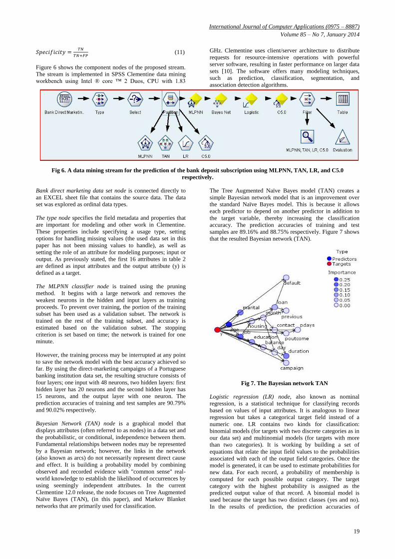
Figure 6 shows the component nodes of the proposed stream.

The stream is implemented in SPSS Clementine data mining

workbench using Intel ® core ™ 2 Duos, CPU with 1.83

GHz. Clementine uses client/server architecture to distribute

requests for resource-intensive operations with powerful

server software, resulting in faster performance on larger data

sets [10]. The software offers many modeling techniques,

such as prediction, classification, segmentation, and

association detection algorithms.

Fig 6. A data mining stream for the prediction of the bank deposit subscription using MLPNN, TAN, LR, and C5.0

respectively.

Bank direct marketing data set node is connected directly to

an EXCEL sheet file that contains the source data. The data

set was explored as ordinal data types.

The type node specifies the field metadata and properties that

are important for modeling and other work in Clementine.

These properties include specifying a usage type, setting

options for handling missing values (the used data set in this

paper has not been missing values to handle), as well as

setting the role of an attribute for modeling purposes; input or

output. As previously stated, the first 16 attributes in table 2

are defined as input attributes and the output attribute (y) is

defined as a target.

The MLPNN classifier node is trained using the pruning

method. It begins with a large network and removes the

weakest neurons in the hidden and input layers as training

proceeds. To prevent over training, the portion of the training

subset has been used as a validation subset. The network is

trained on the rest of the training subset, and accuracy is

estimated based on the validation subset. The stopping

criterion is set based on time; the network is trained for one

minute.

However, the training process may be interrupted at any point

to save the network model with the best accuracy achieved so

far. By using the direct-marketing campaigns of a Portuguese

banking institution data set, the resulting structure consists of

four layers; one input with 48 neurons, two hidden layers: first

hidden layer has 20 neurons and the second hidden layer has

15 neurons, and the output layer with one neuron. The

prediction accuracies of training and test samples are 90.79%

and 90.02% respectively.

Bayesian Network (TAN) node is a graphical model that

displays attributes (often referred to as nodes) in a data set and

the probabilistic, or conditional, independence between them.

Fundamental relationships between nodes may be represented

by a Bayesian network; however, the links in the network

(also known as arcs) do not necessarily represent direct cause

and effect. It is building a probability model by combining

observed and recorded evidence with "common sense" real-

world knowledge to establish the likelihood of occurrences by

using seemingly independent attributes. In the current

Clementine 12.0 release, the node focuses on Tree Augmented

Naïve Bayes (TAN), (in this paper), and Markov Blanket

networks that are primarily used for classification.

The Tree Augmented Naïve Bayes model (TAN) creates a

simple Bayesian network model that is an improvement over

the standard Naïve Bayes model. This is because it allows

each predictor to depend on another predictor in addition to

the target variable, thereby increasing the classification

accuracy. The prediction accuracies of training and test

samples are 89.16% and 88.75% respectively. Figure 7 shows

that the resulted Bayesian network (TAN).

Fig 7. The Bayesian network TAN

Logistic regression (LR) node, also known as nominal

regression, is a statistical technique for classifying records

based on values of input attributes. It is analogous to linear

regression but takes a categorical target field instead of a

numeric one. LR contains two kinds for classification:

binomial models (for targets with two discrete categories as in

our data set) and multinomial models (for targets with more

than two categories). It is working by building a set of

equations that relate the input field values to the probabilities

associated with each of the output field categories. Once the

model is generated, it can be used to estimate probabilities for

new data. For each record, a probability of membership is

computed for each possible output category. The target

category with the highest probability is assigned as the

predicted output value of that record. A binomial model is

used because the target has two distinct classes (yes and no).

In the results of prediction, the prediction accuracies of

International Journal of Computer Applications (0975 – 8887)

Volume 85 – No 7, January 2014

20

training and test samples are 90.09% and 90.43%

respectively.

C5.0 node is trained and tested using a simple model with the

partitioned data. The minimum number of samples per node is

set to be 2 and the decision tree with 12 in depth. It will

examine the importance rate of the predictors before starting

to build the model by winnow attribute's option. Predictors

that are found to be irrelevant are then removed from the

model-building process [2]. The prediction accuracies of

training and test samples are 93.23% and 90.09%

respectively.

Filter, Analysis and Evaluation nodes are used to select and

rename the classifier outputs in order to compute the

performance statistical measures and to graph the evaluation

charts. Table 5 shows the numerical illustration of the

importance of the attributes with respect to models MLPNN,

TAN, LR and C5.0.

TABLE 5 THE IMPORTANCE OF ATTRIBUTES RELATED TO THE MLPNN AND C5.0

Models Importance

Att

rib

ute

s

Ag

e

Jo

b

Ma

rita

l

Ed

uca

tio

n

Defa

ult

Bala

nce

Ho

usi

ng

Loa

n

Co

nta

ct

Da

y

Mo

nth

Du

ra

tio

n

Ca

mp

aig

n

Pd

ay

s

Prev

iou

s

Po

utc

om

e

MLPNN 0.0223 0.0504 0.021 0.0247 0.0062 0.0083 0.0226 0.0174 0.0555 0.0478 0.1762 0.326 0.0198 0.0376 0.0142 0.15

TAN 0.2921 0.1902 0.1482 0.0955 0.018 0.0056 0.0107 0.0674 0 0 0 0.148 0.0217 0 0.0024 0

LR ------ 0.0344 0.0139 0.0136 ----- ------ 0.0613 0.0172 0.0807 0 0.0531 0.499 0.0346 ------ 0.0131 0.179

C5.0 0 0.0186 0.0301 0 ----- 0.0237 0 0.0152 0 0 0 0.722 0.0206 0.0095 0.0072 0.153

The table illustrates that the attribute Duration is the most

important for three examined models. In MLPNN, the ratio is

0.339, 0.499 for LR and in C5.0 is 0.722 that they are highest

ratios among all the other attributes; however, the attribute

Age is nominated by TAN with ratio 0.292. The attribute

Default is removed by LR and C5.0, also Age, Balance, Pdays

attributes are removed by LR only because it is trivial or not

has any degree of importance with respect these models.

However, some attributes are not removed; nevertheless, they

measured from zero because their importance is very low and

rounded to zero, such as Contact, Day, Month in models TAN

and C5.0, Pdays, Poutcome attributes only in TAN and Day in

LR again rounded to zero. These all ratios are illustrated in

Figure 8.

Fig 8. The most importance of attributes based on MLPNN, TAN, LR, and C5.0

Figure 9 shows the cumulative charts of the four models for

training and test subsets. The higher lines indicate better

models, especially on the left side of the chart. The four

curves are same for the test subset and almost identical to the

training one. This figure shows that MLPNN line crowed LR

and C5.0 lines to reach the best line in the training subsets in

some positions; even so, TAN leaves them and individually

stayed alone. In the same contest, the success is observed for

the alike three models MLPNN, LR, and C5.0 in the testing

subset and TAN stayed far from them.

Fig 9. The cumulative gains charts of the four models for training and test subsets.

0

0.1

0.2

0.3

0.4

0.5

0.6

0.7

0.8

MLPNN

TAN

LR

C5.0

International Journal of Computer Applications (0975 – 8887)

Volume 85 – No 7, January 2014

21

The predictions of all models are compared to the original

classes to identify the values of true positives, true negatives,

false positives and false negative. These values have been

computed to construct the confusion matrix as tabulated in

Table 6 where each cell contains the raw number of cases

classified for the corresponding combination of desired and

actual classifier outputs.

TABLE 6 The Confusion Matrices of MLPNN, TAN, LR and C5.0 Models for Training and Testing Subsets

Model Training Data Testing Data

Desired output Yes No Desired output Yes No

MLPNN Yes TP=1,771 FP=1,941 Yes TP=719 FP=858

No FN=926 TN=26,951 No FN=437 TN=11,608

TAN Yes 1,374 2,338 Yes 535 1,042

No 1,085 26,792 No 490 11,555

LR Yes 1,270 2,442 Yes 578 999

No 689 27,188 No 304 11,741

C5.0 Yes 2,258 1,454 Yes 740 837

No 684 27,193 No 513 11,532

The values of the statistical parameters (sensitivity, specificity

and total classification accuracy) of the four models were

computed and presented in Table 7. Accuracy, Sensitivity and

Specificity approximate the probability of the positive and

negative labels being true. They assess the usefulness of the

algorithm on a single model. By using the results shown in

Table 7, it can be seen that the sensitivity, specificity and

classification accuracy of all models has achieved 94.92%

success of training samples.

In this table, MLPNN model has accuracy 90.92% for training

samples and 90.49% of tested samples, 89.16% and 88.75 for

training and testing samples according to TAN. The

classification accuracy of LR model is 90.09% and 90.43%

for training and testing samples, also C5.0 model has 93.23%

of training samples and 90.09% of testing samples, and so on.

The highest value in training samples is appeared for C5.0;

nevertheless, the highest percentage of testing is in the cell of

MLPNN for accurate classification. Simultaneously, the

sensitivity analysis takes the highest percentage in C5.0 of the

training samples 76.75%; however, for testing samples the

highest value is 65.53% for LR.

TABLE 7 PERCENTAGES OF THE STATISTICAL

MEASURES OF MLPNN, TAN, LR AND C5.0 FOR

TRAINING AND TESTING SUBSETS

Model Partition Accuracy Sensitivity Specificity

MLPNN Training 90.92% 65.66% 93.28%

Testing 90.49% 62.20% 93.12%

TAN Training 89.16% 55.87% 91.97%

Testing 88.75% 52.19% 91.73%

LR Training 90.09% 64.83% 91.76%

Testing 90.43% 65.53% 92.16%

C5.0 Training 93.23% 76.75% 94.92%

Testing 90.09% 59.06% 93.23%

Last but not least, the specificity measure has C5.0 with the

highest values in training samples 94.92% and 93.23% for

testing samples. From the previews, C5.0 is the best in

accuracy, sensitivity, and specificity analysis of training

samples; however, the MLPNN is the best for accuracy; LR

takes the best percentage for sensitivity, and C5.0 return to be

the best in specificity analysis of testing samples.

9. CONCLUSION Bank direct marketing and business decisions are more

important than ever for preserving the relationship with the

best customer. To success and survival, the business there is a

need for customer care and marketing strategies. Data mining

and predictive analytics can provide help in such marketing

strategies. Its applications are influential in almost every field

containing complex data and large procedures. It has proven

the ability to reduce the number of false positives and false-

negative decisions. This paper has been evaluating and

comparing the classification performance of four different

data mining techniques' models MPLNN, TAN, LR and C5.0

on the bank direct marketing data set to classify for bank

deposit subscription. The purpose is increasing the campaign

effectiveness by identifying the main characteristics that

affect the success (the deposit subscribed by the client). The

classification performances of the four models have been

using three statistical measures; Classification accuracy,

sensitivity and specificity. This data set has partitioned into

training and test by the ratio 70% and 30%, respectively.

Experimental results have shown the effectiveness of models.

C5.0 has achieved slightly better performance than MLPNN,

LR and TAN. Importance analysis has shown that attribute

"Duration" in C5.0, LR, and MLPNN models have achieved

the most important attribute; however, the attribute Age is the

only assessed as more important than the other attributes by

TAN.

10. REFERENCES [1] A. Floares., A. Birlutiu. “Decision Tree Models for

Developing Molecular Classifiers for Cancer Diagnosis”.

WCCI 2012 IEEE World Congress on Computational

Intelligence June, 10-15, 2012 - Brisbane, Australia.

[2] Adem Karahoca, Dilek Karahoca and Mert Şanver, "Data

Mining Applications in Engineering and Medicine",

ISBN 978-953-51-0720-0, In Tech, August 8, 2012.

[3] B. Chaudhuri and U. Bhattacharya.” Efficient training

and improved performance of multilayer perceptron in

International Journal of Computer Applications (0975 – 8887)

Volume 85 – No 7, January 2014

22

pattern classification”. Neuro computing, 34, pp11–27,

September 2000.

[4] D.G. Kleinbaum and M. Klein, Logistic Regression,

Statistics for Biology and Health, DOI 10.1007/978-1-

4419-1742-31, Springer Science Business Media, LLC

2010.

[5] Derrig, Richard A., and Louise A. Francis,

"Distinguishing the Forest from the TREES: A

Comparison of Tree-Based Data Mining

Methods," Variance 2:2, 2008, pp. 184-208.

[6] Domínguez-Almendros S. “LOGISTIC REGRESSION

MODELS”. Allergol Immunopathol (Madr). 2011.

doi:10.1016/j.aller.2011.05.002.

[7] Eniafe Festus Ayetiran, “A Data Mining-Based Response

Model for Target Selection in Direct Marketing”,

I.J.Information Technology and Computer Science, 2012,

1, 9-18.

[8] Harry Zhang., Liangxiao Jiang., Jiang Su. “Augmenting

Naïve Bayes for Ranking”. Published in: Proceeding of

ICML '05 Proceedings of the 22nd international

conference on Machine learning Pages 1020 – 1027,

2005.

[9] Ho, T.B. (nd). “Knowledge Discovery and Data Mining

Techniques and Practice”. 2006, Available on:

www.netnam.vn/unescocourse/knowlegde/knowfrm.htm

[10] http://archive.ics.uci.edu/ml (The UCI Machine Learning

Repository is a collection of databases).

[11] http://en.wikipedia.org/wiki/Direct_marketing.

Wikipedia has a tool to generate citations for particular

articles related to direct marketing.

[12] http://en.wikipedia.org/wiki/Naïve_Bayes_classifier

Wikipedia has a tool to generate citations for particular

articles related to Naïve Bayes classifier.

[13] http://en.wikipedia.org/wiki/Neural_network#History of

the neural network analogy Wikipedia has a tool to

generate citations for particular articles related to Neural

Network.

[14] http://rimarcik.com/en/navigator/nlog.html Personale

web site introducing many statistics tools illustrated by

Marian Rimarcik.

[15] http://www2.cs.uregina.ca/~dbd/cs831/index.html

Knowledge Discovery in Databases 2012.

[16] J. W. Han and M. Kamber. Data mining concepts and

techniques, The 2nd edition, Morgan Kaufmann

Publishers, San Francisco, CA, 2006.

[17] L. Ma and K. Khorasani. “New training strategy for

constructive neural networks with application to

regression problems”. Neural Networks, 17,589-609,

2004.

[18] O'guinn, Thomas.” Advertising and Integrated Brand

Promotion”. Oxford Oxfordshire: Oxford University

Press. p. 625. ISBN 978-0-324-56862-2. , 2008.

[19] Ou, C., Liu, C., Huang, J. and Zhong, N. ‘One Data

mining for direct marketing’, Springer-Verlag Berlin

Heidelberg, pp. 491–498., 2003.

[20] Petrison, L. A., Blattberg, R. C. and Wang, P. ‘Database

marketing: Past present, and future’, Journal of Direct

Marketing, 11, 4, 109–125, 1997.

[21] R. Nisbet, J. Elder and G. Miner. Handbook of statistical

analysis and data mining applications. Academic Press,

Burlington, MA, 2009.

[22] S. Moro, R. Laureano and P. Cortez. Using Data Mining

for Bank Direct Marketing: An Application of the

CRISP-DM Methodology. In P. Novais et al. (Eds.),

Proceedings of the European Simulation and Modelling

Conference - ESM'2011, pp. 117-121, Guimarães,

Portugal, October, 2011.

[23] Su-lin PANG, Ji-zhang GONG, C5.0 Classification

Algorithm and Application on Individual Credit

Evaluation of Banks, Systems Engineering - Theory &

Practice, Volume 29, Issue 12, Pages 94–104, December

2009.

[24] T. Munkata, “Fundamentals of new artificial

intelligence,” 2nd edition, London, Springer-Verlag,

2008.

[25] TIAN YuBo, ZHANG XiaoQiu, and ZHU RenJie.

“Design of Waveguide Matched Load Based on

Multilayer Perceptron Neural Network”. Proceedings of

ISAP, Niigata, Japan 2007.

[26] Tom M. Mitchell. “Machine Learning”. Copyrightc

2005-2010. Second edition of the textbook. Chapter 1, all

rights reserved. January 19, 2010 McGraw Hill. 119

ACM 2005, ISBN 1-59593-180-5.

[27] Freeman WJ. “The physiology of perception”. University

of California, Berkeley. Sci Am. 1991 Feb;264(2):78-85.

[28] Craven MW, Shavlik JW. “Understanding time series

networks: a case study in rule extraction”. Int J Neural

Syst. 1997 Aug;8(4):373-84.

IJCATM : www.ijcaonline.org