Embed Size (px)
Citation preview

An Investigation Into Dynamical Bandwidth
Management and Bandwidth Redistribution Using A
Pool of Cooperating Interfacing Gateways And A
Packet Sniffer In Mobile Cloud Computing:
Prepared by:
Lukas Ndakola Shuuya
SHYLUK001 Department of Electrical Engineering
University of Cape Town
Prepared for:
Dr. Fred Nicolls Department of Electrical Engineering
University of Cape Town
March 2021
Minor dissertation paper submitted to the Department of Electrical Engineering at the
University of Cape Town in partial fulfilment of the academic requirements for the qualification
of a Master of Engineering in Telecommunications.
Key Words: Mobile Cloud Computing, Quality of Service, Packet Sniffing, Dynamical
Bandwidth Management, Bandwidth Redistribution, Interfacing Gateways.
Universi
ty of
Cape T
own

The copyright of this thesis vests in the author. No quotation from it or information derived from it is to be published without full acknowledgement of the source. The thesis is to be used for private study or non-commercial research purposes only.
Published by the University of Cape Town (UCT) in terms of the non-exclusive license granted to UCT by the author.
Universi
ty of
Cape T
own

i
Declaration
1. I know that plagiarism is wrong. Plagiarism is to use another's work and pretend that it is
one's own.
2. I have used the IEEE convention for citation and referencing. Each contribution to, and
quotation in, this final year project report from the work(s) of other people, has been
attributed and has been cited and referenced.
3. This final year project report is my own work.
4. I have not allowed, and will not allow, anyone, to copy my work with the intention of
passing it off as their own work or part thereof
Name: Lukas Ndakola Shuuya
Signature: Date: 21 March 2021

ii
Acknowledgements
First and foremost, I thank the Almighty Heavenly Father for the experience and for carrying
me yet again through another significant undertaking in my life.
This research would not have been possible had it not been for the support rendered by the
following people:
i. My supervisors, Dr. Alexandru Murgu and Dr. Fred Nicolls, for their guidance and
advice during the project.
ii. My son Holden for his patience, consistent understanding, and the sacrifices he endured
when this work was being undertaken.
iii. My mum and brothers for their prayers and pleasing encouragement. Their support kept
me going.
iv. My employer, Telecom Namibia, for allowing me time off work to attend to my studies
as and when required.
v. My colleague, Mr. Heikki Nakanyala for his willingness to help out during the network
setup. I appreciate the time and effort that he has put into this.
May the Almighty Father bless them abundantly!
I dedicate this research project to my late son and firstborn (Jayden Liinekela Shuuya), who
untimely passed on on 25 April 2019 and could unfortunately not see me complete this
significant undertaking in my life. May your soul continue to rest in eternal peace, son.
This research project is also dedicated to my late father and namesake (Lukas Ndakola Shuuya),
who passed on on 03 February 2019 and could, unfortunately, also not see me complete this
significant undertaking in my life. May your soul continue to rest in eternal peace, dad.

iii
Glossary
ACK – Acknowledgement
ARP – Address Resolution Protocol
AS – Autonomous System
CC - Cloud Computing
CPU – Central Processing Unit
CSP – Cloud Service Provider
DHCP – Dynamic Host Control Protocol
DiffServ – Differentiated Service
DNS – Domain Name System
DSCP – Differentiated Service Code Point
ECN – Explicit Congestion Notification
Gbps - Gigabits per second
GHz - Giga Hertz
GNS3 – Graphical Network Simulator - 3
IETF – International Engineering Task Force
IntServ – Integrated Service
IOS - Internetwork Operating System
IP – Internet Protocol
ITU – International Telecommunications Union
Kbps - Kilobits per second
LAN – Local Area Network
MAC – Media Access Control
Mbps – Megabits per second
MC – Mobile Computing
MCC – Mobile Cloud Computing
NAT – Network Address Translation
NIC – Network Interface Card
OS – Operating System
PC – Personal Computer
QoE – Quality of Experience
QoS – Quality of Service
RAM – Random Access Memory
RTT – Round Trip Time
RFC – Request For Comment
TCP – Transport Control Protocol
ToS – Type of Service
UDP – User Datagram Protocol
VM – Virtual Machine
WAN – Wide Area Network

iv
Abstract
Mobile communication devices are increasingly becoming an essential part of almost every
aspect of our daily life. However, compared to conventional communication devices such as
laptops, notebooks, and personal computers, mobile devices still lack in terms of resources such
as processor, storage and network bandwidth. Mobile Cloud Computing is intended to augment
the capabilities of mobile devices by moving selected workloads away from resource-limited
mobile devices to resource-intensive servers hosted in the cloud.
Services hosted in the cloud are accessed by mobile users on-demand via the Internet using
standard thick or thin applications installed on their devices. Nowadays, users of mobile devices
are no longer satisfied with best-effort service and demand QoS when accessing and using
applications and services hosted in the cloud. The Internet was originally designed to provide
best-effort delivery of data packets, with no guarantee on packet delivery. Quality of Service
has been implemented successfully in provider and private networks since the Internet
Engineering Task Force introduced the Integrated Services and Differentiated Services models.
These models have their legacy but do not adequately address the Quality of Service needs in
Mobile Cloud Computing where users are mobile, traffic differentiation is required per user,
device or application, and packets are routed across several network domains which are
independently administered.
This study investigates QoS and bandwidth management in Mobile Cloud Computing and
considers a scenario where a virtual test-bed made up of GNS3 network software emulator,
Cisco IOS image, Wireshark packet sniffer, Solar-Putty, and Firefox web browser appliance is
set up on a laptop virtualized with VMware Workstation 15 Pro. The virtual test-bed is in turn
connected to the real world Internet via the host laptop’s Ethernet Network Interface Card.
Several virtual Firefox appliances are set up as end-users and generate traffic by launching web
applications such as video streaming, file download and Internet browsing. The traffic
generated by the end-users and bandwidth used is measured, monitored, and tracked using a
Wireshark packet sniffer installed on all interfacing gateways that connect the end-users to the
cloud. Each gateway aggregates the demand of connected hosts and delivers Quality of Service
to connected users based on the Quality of Service policies and mechanisms embedded in the
gateway.
Analysis of the results shows that a packet sniffer deployed at a suitable point in the network
can identify, measure and track traffic usage per user, device, or application in real-time. The
study has also demonstrated that when deployed in the gateway connecting users to the cloud,
it provides network-wide monitoring and traffic statistics collected can be fed to other
functional components of the gateway where a dynamical bandwidth management scheme can
be applied to instantaneously allocate and redistribute bandwidth to target users as they roam
around the network from one location to another. This approach is however limited and
ensuring end-to-end Quality of Service requires mechanisms and policies to be extended across
all network layers along the traffic path between the user and the cloud in order to guarantee a
consistent treatment of traffic.

v
Table of Contents
Declaration ································································································· i
Acknowledgements······················································································· ii
Glossary ··································································································· iii
Abstract ··································································································· iv
Table of Figures ························································································ viii
Table of Tables ···························································································· x
1 Introduction ·························································································· 1
Background ······················································································ 1
1.1.1 Mobile Cloud Computing ································································ 2
1.1.2 Quality of Service ········································································· 2
1.1.3 Packet Sniffing ············································································ 3
1.1.4 Bandwidth Management ································································· 4
1.1.5 Interdomain Management ································································ 5
Problem Statement ············································································· 5
Objectives of This Study ······································································ 6
Problems Investigated ········································································· 6
Purpose of Study ················································································ 7
Study Motivation ··············································································· 7
Scope and Limitations ········································································· 8
1.7.1 Scope ························································································ 8
1.7.2 Limitations ················································································· 8
Knowledge Contribution ······································································ 9
Development Plan ·············································································· 9
2 Literature Review ·················································································· 11
Introduction····················································································· 11
Cloud Computing ·············································································· 11
2.2.1 Essential Characteristics ································································ 11
2.2.2 Service Models ··········································································· 12
2.2.3 Deployment Models ····································································· 13
2.2.4 Advantages of Cloud Services ························································· 14
Mobile Computing ············································································ 14
Mobile Cloud Computing ···································································· 15
2.4.1 Overview of Mobile Cloud Computing ··············································· 16
2.4.2 Benefits of Mobile Cloud Computing ················································ 17
2.4.3 Mobile Cloud Computing Challenges ················································ 18

vi
Traffic Types ··················································································· 19
2.5.1 Voice ······················································································· 19
2.5.2 Video ······················································································· 19
2.5.3 Data ························································································ 20
Autonomous System ·········································································· 23
Service Level Agreement····································································· 24
QoS Overview ················································································· 24
2.8.1 QoS Metrics ··············································································· 25
2.8.2 QoS Framework ·········································································· 26
QoS Mechanisms ·············································································· 26
QoS Models ···················································································· 27
2.10.1 Best Effort ················································································· 27
2.10.2 Integrated Services (IntServ) ··························································· 27
2.10.3 Differentiated Services (DiffServ) ····················································· 28
Bandwidth Monitoring ········································································ 29
Packet Sniffing ················································································· 30
Packet Sniffer Structure ······································································ 31
2.13.1 Packet Header-based Sniffing ·························································· 34
Bandwidth Control ············································································ 36
Quality of Service Monitoring ······························································· 37
Review of Previous Related Studies: ······················································· 38
3 System Model ······················································································· 40
Introduction····················································································· 40
MCC System Model ·········································································· 40
Service Delay ·················································································· 42
Packet Sniffing ················································································· 43
Bandwidth Redistribution ···································································· 43
Dynamical Bandwidth Allocation Algorithm ············································· 44
4 Development Tools ················································································ 50
Introduction····················································································· 50
Host Machine Specifications ································································ 50
Software Tools installed in Virtual Network Lab ········································· 51
4.3.1 VMware Workstation 15 Pro ··························································· 51
4.3.2 Cisco Router Internetwork Operating System ······································· 52
4.3.3 Graphical Network Simulator 3 ························································ 53
4.3.4 Wireshark ················································································· 55
4.3.5 Firefox Appliance ········································································ 57

vii
4.3.6 Solar-Putty ················································································ 58
Implementation of Testbed Environment ·················································· 58
GNS3 Topology ··············································································· 60
4.5.1 Interior Gateway Protocol ······························································ 60
4.5.2 Host IP address Allocation ····························································· 60
4.5.3 Router R6 Inventory ····································································· 61
4.5.4 Router R2 Inventory ····································································· 61
4.5.5 Router R1 Inventory ····································································· 62
4.5.6 Cloud Node ··············································································· 63
Quality of Service ············································································· 64
QoS Mechanisms ·············································································· 65
4.7.1 Classification ············································································· 65
4.7.2 Marking···················································································· 65
4.7.3 Policing ···················································································· 66
4.7.4 Queuing···················································································· 66
Packet Sniffing per Device ··································································· 66
Concluding Remarks ·········································································· 67
5 Results and Analysis··············································································· 68
Introduction····················································································· 68
Scenario 1: Device-1 Connected to R1 ····················································· 68
Scenario 2: Device-1 Connected to R2 ····················································· 73
Scenario 3: Multiple Devices Connected ·················································· 77
Concluding remarks ··········································································· 92
6 Conclusion and Recommendation ······························································ 93
Conclusion ······················································································ 93
6.1.1 Interfacing gateways ····································································· 93
6.1.2 Packet Sniffing ··········································································· 93
6.1.3 QoS Monitoring and Provisioning ····················································· 94
6.1.4 Dynamical Bandwidth Allocation ····················································· 94
Recommendations ············································································· 95
6.2.1 Using A Unique Identifier That Does Not Change ································· 95
6.2.2 Adding Packet Sniffers In The Access And Peering Points ······················· 95
6.2.3 Adding Mobility To The Cloud ························································ 95
6.2.4 Adding Support For Fully Intelligent And Programmable Network ············· 96
6.2.5 Adding Support For Deep Packet Inspection ········································ 96
7 References ··························································································· 97

viii
Table of Figures
Figure 1: IMT Global Mobile Subscriptions Estimation [2]. .................................................... 1 Figure 2: Sniffing Process Flow ................................................................................................ 4 Figure 3: SLA Architecture in TCP/IP Networks ..................................................................... 5
Figure 4: Scope of Controls between Provider and Consumer [4]. ........................................ 13 Figure 5: MCC Architecture [18], [19]. .................................................................................. 16 Figure 6: Global IP Traffic Forecast 2017-2022 [23]. ............................................................ 21 Figure 7: User-centric QoS Requirements [24]. ..................................................................... 21 Figure 8: Architectural Framework for QoS Support [24] ...................................................... 26
Figure 9: Structure of a Packet Sniffer [32]. ........................................................................... 32 Figure 10: Standard PCAP Application Flow [32]. ................................................................ 33 Figure 11: Data Encapsulation in a TCP/IP Network [32]. .................................................... 33 Figure 12: Ethernet Packet Structure [27]. .............................................................................. 34
Figure 13: IPV4 Packet Header Structure [27]. ...................................................................... 34 Figure 14: IPV6 Packet Header Structure [27]. ...................................................................... 35 Figure 15: MCC Model. .......................................................................................................... 40
Figure 16: Simulation Model Before U2 Movement. ............................................................. 44 Figure 17: Simulation Model After U2 Movement. ................................................................ 45 Figure 18: Algorithm Transmission Diagram ......................................................................... 47 Figure 19: Algorithm Flow Chart ............................................................................................ 48
Figure 20: Host Machine Specifications. ................................................................................ 50 Figure 21: Host Machine Processors. ...................................................................................... 51
Figure 22: GNS3 GUI. ............................................................................................................ 54 Figure 23: Screenshot of Wireshark GUI. ............................................................................... 56 Figure 24: Solar-PuTTY. ........................................................................................................ 58
Figure 25: Test Bed Installation Process ................................................................................. 59 Figure 26: Virtual Router R6 Inventory. ................................................................................. 61
Figure 27: Virtual Router R2 Inventory. ................................................................................. 62 Figure 28: Virtual Router R1 Inventory. ................................................................................. 63
Figure 29: GNS3 Cloud Node. ................................................................................................ 63 Figure 30: Start Capturing Packets. ........................................................................................ 64 Figure 31: Scenario 1 GNS3 Topology. .................................................................................. 68
Figure 32: Scenario 1 Host Firefox-1 to R1 Capture. ............................................................. 69 Figure 33: Scenario 1 Firefox-1 GNS3 Node Properties. ....................................................... 71
Figure 34: Scenario 1 R1 to R6 Capture. ................................................................................ 71 Figure 35: Scenario 2 GNS3 Topology. .................................................................................. 73 Figure 36: Scenario 2 Firefox-1 to R2 Capture. ...................................................................... 74
Figure 37: Scenario 2 Firefox-1 GNS3 Node Properties. ....................................................... 75 Figure 38: Scenario 2 R2 to R6 Capture. ................................................................................ 76 Figure 39: GNS3 Topology for Scenario 3. ............................................................................ 77
Figure 40: Scenario 3 R6 to NAT-0 Capture. ......................................................................... 78 Figure 41: Scenario 3 R6 to NAT-0 Capture. ......................................................................... 79 Figure 42: Scenario 3 R6 to NAT-0 Capture. ......................................................................... 80 Figure 43: Scenario 3 R2 to R6 Capture. ................................................................................ 81 Figure 44: Scenario 3 R6 to NAT-0 Capture. ......................................................................... 82 Figure 45: Firefox-1 Web Browsing. ...................................................................................... 83 Figure 46: Firefox-1 Web Browsing. ...................................................................................... 83 Figure 47: Firefox-2 Web Browsing. ...................................................................................... 84

ix
Figure 48: Netflix Video Streaming Attempt. ......................................................................... 85
Figure 49: YouTube Video Streaming Attempt. ..................................................................... 85
Figure 50: Firefox-2 Version Upgrade Attempt. ..................................................................... 86 Figure 51: Firefox-3 Version Upgrade Attempt. ..................................................................... 86 Figure 52: Firefox Ping Result. ............................................................................................... 87 Figure 53: Firefox-1 Internet Upstream Throughput Capture. ................................................ 88 Figure 54: Firefox-1 Internet Downstream Throughput Capture. ........................................... 89
Figure 55: Upstream Round-Trip Time Graph. ...................................................................... 90 Figure 56: Downstream Round-Trip Time Graph. ................................................................. 91
x
Table of Tables
Table 1: ITU QoS Classes [24]. .............................................................................................. 22 Table 2: Minimum Application Download Speed. ................................................................. 23 Table 3: Differences between the three QoS models [29] ....................................................... 29

1
Chapter 1
1 Introduction
Background
During the last decade, we have witnessed the proliferation of mobile devices and web-based
applications. When one looks around, you are likely to see someone glued to the screen of a
mobile device. The mass adoption of mobile devices underscores society’s increasing reliance
on mobile devices for many facets of daily life. Compared to fixed communication devices,
mobile devices are often preferred because they offer users the benefits of convenience,
flexibility, and portability. Users of mobile devices generally expect them to function like
conventional digital communication devices such as personal computers, notebooks, and
laptops. However, compared to laptops and personal computers, mobile devices still lack in
terms of resources such as processor, storage, and network bandwidth [1].
To illustrate the extent to which mobile devices are being adopted across the world, the
International Telecommunications Union (ITU) estimates that the number of mobile
subscriptions globally is expected to grow from about 11 billion in 2020 to about 17 billion by
2030 as depicted in the figure below.
Figure 1: IMT Global Mobile Subscriptions Estimation [2].
On the other hand, the United Nations estimates that the world's human population is expected
to be about 7.5 billion by 2020 and grow to 8.5 billion by 2030 [3]. This means that by 2030,
the number of mobile subscriptions is expected to be about double the world’s population, with
most subscriptions being undertaken using a Smartphone as shown in Figure 1 above.
Mobile devices are still considered to be resource-limited computing devices. For instance,
compared to conventional laptops and personal computers, they still face various challenges

2
such as shorter battery life, lower processing speed, smaller storage capacity, and lower network
bandwidths, which affects their use [1]. For instance, battery life restricts their working time,
while storage and processing inhibit the ability of the device to support the execution of
computationally intensive applications. Mobile Cloud Computing (MCC) technology provides
the ability to enhance the capability of mobile devices by moving selected workloads away
from resource-limited mobile devices to resource-intensive servers hosted in the cloud. In what
follows next, the MCC concept is introduced.
1.1.1 Mobile Cloud Computing
The Mobile Cloud Computing Forum as cited by [4, p. 4] defines MCC as follows: “Mobile
Cloud Computing in its simplest refers to an infrastructure where both data storage and data
processing happens outside of the mobile device. Mobile cloud applications move the
computing power and data processing away from mobile phones and into the cloud, bringing
applications and mobile cloud to not just smartphone users but a much broader range of mobile
subscribers”. From the foregoing definition, MCC augment the capability of mobile devices
and enables new types of services and reduces the need for a user to have a mobile device with
a powerful processor, and large storage because selected resource-intensive workloads can be
performed in the cloud instead of on the mobile device. For instance;
• It enables new types of applications and business models that impact almost every aspect
of our daily life in areas such as education, agriculture, transportation, commerce,
healthcare, safety, security, smart home, smart city, and social interaction [5].
• It allows large volumes of data to be transferred from smart mobile devices to high-capacity
servers hosted in the cloud for storage [1].
• It enables data processing workloads to be moved away from smart mobile devices to
powerful servers hosted in the cloud for execution [1].
Services hosted in the cloud are accessed by mobile users on-demand using the Transmission
Control Protocol/Internet Protocol (TCP/IP) suite. The Internet was originally designed to
provide best-effort delivery of data packets, with no guarantee on packet delivery. Users
nowadays are no longer satisfied with best-effort service and demand Quality of Service (QoS)
when accessing and using applications and services hosted in the cloud. In what follows next,
the QoS concept is introduced.
1.1.2 Quality of Service
QoS is a well-studied topic is both industry and academia. The ITU-T in its recommendation
(Rec. E.800) defines QoS as the “totality of characteristics of a telecommunications service
that bear on its ability to satisfy stated and implied needs of the user of the service” [6, p. 2].
The above definition is very broad and takes a service view and points out that users of a
telecommunications service have expectations that needs to be met by the network offering the
service. The Internet Engineering Task Force (IETF) in RFC 2386 defines QoS as “a set of
service requirements to be met by the network while transporting a flow” [7, p. 2]. The IETF
also distinguishes between static and dynamic QoS and states in RFC 2216 that “a network with
dynamically controllable quality of service allows individual application sessions to request
network packet delivery characteristics according to their perceived needs, and may provide
different qualities of service to different applications” [8, p. 2]. From the foregoing, QoS is
concerned with the ability of a telecommunications network to identify and differentiate
between different types of traffic and subsequently provide priority treatment to certain types

3
of traffic in order to guarantee a prescribed level of performance. In TCP/IP networks,
performance can be expressed in terms of parameters such as:
• Throughput (bandwidth),
• Jitter (delay variation),
• Packet loss rate,
• Latency (delay), etc
The Internet by default treats all customers and all traffic in the same way and offers no
performance or quality guarantees for any traffic flow [9]. This study deals with the issue of
dynamical bandwidth management as a mechanism to ensure QoS in MCC. To manage
bandwidth usage in a network, bandwidth usage needs to be measurement and control at a level
of abstraction appropriate for the service concerned. Bandwidth usage data in a TCP/IP network
can be obtained from target devices and applications using various data acquisition methods
such as Simple Network Management Protocol (SNMP), xFlow, and Packet Sniffing. SNMP
data can provide vital information regarding bandwidth usage on a port-by-port basis but does
not differentiate traffic by type of service or protocol type, which is essential in MCC. xFlow
requires special configuration in the routers’ setup to direct them as to where to send the flow
data. This is also limited considering that not all MCC players will have administrative
privileges to routers. A packet sniffer can operate passively by inspecting all IP packets passing
through the Network Interface Card of a communications link. It does, generally, not require
special configuration in routers to instruct them to send data anywhere, save for the case where
port mirroring techniques are used.
Given the foregoing, packet sniffing appears to be a noble idea that can meet the needs of
various players in MCC such as Internet Service Providers (ISP), Cloud Service Providers
(CSP), and Cloud Brokers. Packet sniffing is therefore investigated in this study as a mechanism
to collect bandwidth usage data and is briefly introduced below.
1.1.3 Packet Sniffing
Packet sniffing is the process of using a software tool or hardware device, called a sniffer, to
capture copies of packets that are transmitted over a communications link and subsequently
analysing their content in order to acquire insight into the packets [8], [9]. As discussed further
in Chapter 2, a packet header contains vital information about the communication and consists
of information such as:
• The source address of the packet,
• The destination address of the packet,
• The source port of the packet,
• The destination port of the packet, and
• The transport protocol,
The content of each packet captured can be analysed to gain real-time or historical insight that
can be used for various purposes, such as:
• Traffic analysis,
• Troubleshooting network issues,

4
• Network security, and
• Bandwidth management (local area and wide area)
Figure 2 below depicts a typical packet sniffing process flow chart based on information
collated from various sources [10], [8].
Figure 2: Sniffing Process Flow
1.1.4 Bandwidth Management
In the context of this study, bandwidth refers to the amount of data that can be transferred, per
unit of time, from one point to another over a communications link [6]. Whereas bandwidth
management refers to the process of measuring and controlling bandwidth distribution to
devices and applications on a network [8]. One of the main objectives of bandwidth
management is to ensure QoS. On the other hand, dynamical bandwidth management is a form
of bandwidth management in which bandwidth allocation to different classes, applications or
users is varied on demand in order to adapt to instantaneous traffic demand [13]. It enables
flexibility in allocating bandwidth to devices, users and applications and is relevant in MCC
since users are mobile and a dynamical bandwidth management mechanism is required to
ensure that users continue to receive a prescribed level of bandwidth as they move from one
location to another. For instance, a mobile user can subscribe to a certain premium cloud
service, and the CSP may wish to offer the user a certain level of QoS irrespective of the location
where they are accessing the cloud service from. Considering that traffic to services hosted in
the cloud is routed across different network domains, it is essential to study how traffic is routed
between domains, and what needs to be done to ensure QoS between domains. These concepts
are introduced below and discussed further in Chapter 2.

5
1.1.5 Interdomain Management
As introduced in the preceding sections, services in MCC are hosted in the cloud and accessed
via the Internet. The Internet is not one big network but consists of thousands of Autonomous
Systems (AS) that are interconnected and cooperate to route IP packets from source to
destination. An AS is defined as a collection of interconnected networks that belong to a single
administrative domain. In the current routing structure of the Internet, routing of packets
between routers belonging to the same AS is achieved using a routing protocol known as an
Interior Gateway Protocol (IGP), whereas routing of packets between routers belonging to
different ASs is achieved using a routing protocol known as an Exterior Gateway Protocol
(EGP) [14].
QoS across the Internet is still a daunting task. Even though different ASs exchange routing and
reachability information with their peers using an EGP, each System is configured
independently, and routing decisions, routing policies and traffic engineering treatment and
measures made and configured within one ASs do not by default extend to any other AS [14].
Moreover, the Border Gateway Protocol (BGP) used as the de facto EGP does not propagate
any performance or QoS metrics, and therefore provides no support for QoS routing. In a
situation where QoS provisioning needs to be extended between adjacent ASs, such an
arrangement needs to be governed by a prescribed Service Level Agreement (SLA) between
peer Service Providers [14] such as AS-1 and AS-2, or a between Service Provider (AS-1) and
an end user as illustrated in the Figure below.
Figure 3: SLA Architecture in TCP/IP Networks
An SLA architecture is required, and functional elements are needed to measure and implement
such an SLA.
Problem Statement
Users of mobile devices are no longer satisfied with best-effort service and demand QoS when
accessing applications and services hosted in the cloud. The current mechanisms for
provisioning QoS in TCP/IP networks have some limitations and do not adequately meet the
demands of MCC users. These mechanisms need to be reconsidered to meet the challenges
posed by MCC users. Over the years, several researchers have been engaged with the problem
of finding ways to provide end-to-end QoS over the Internet. To deal with the issue of QoS in
MCC, a logical entity called an interfacing gateway has been proposed in recent studies. The
gateway is used to facilitate connectivity between mobile users and the cloud. As opposed to
the traditional cloud model where each user requests bandwidth directly from the cloud, users
instead request bandwidth from the interface gateway to which it is attached. The interface
gateway aggregates the demand for connected devices and requests the required amount of

6
bandwidth from the cloud. This operation is analogous to IntServ where the Resource
Reservation Protocol (RSVP) is used as an underlying mechanism to signal and explicitly
reserve the desired resources for a flow. This can become more complex if the mobility of users
is considered because as users move around from one location to another, the interface gateway
to which they are connected can change, and the aggregate bandwidth requirement of the
interface gateways may also change. As a result, a mobile user may be able to access a cloud
service at one location with good QoS but may find it difficult to access the same service at
another location, even though the user enjoys the same level of QoS in the Radio Access
Network.
This study aims to complement existing research on bandwidth management and QoS in MCC
and investigates a scenario in which a packet sniffer deployed on the interface gateway is used
to measure, monitor, and track bandwidth usage per user, device or application. To ensure
bandwidth allocation and QoS, even as the user roams around the network, each gateway
employs a dynamical bandwidth management algorithm that allocates and redistributes a
prescribed level of bandwidth to a user irrespective of the gateway to which the user is
connected to.
Objectives of This Study
The main research objective of this study is to investigate bandwidth management and QoS in
MCC using interface gateways and a packet sniffer to ensure bandwidth allocation and
redistribution to users as they move around the network in a MCC environment. From this main
objective, the following specific objectives are derived:
1. To review related work in the areas of packet sniffing, bandwidth management, and QoS in
MCC.
2. To design and simulate investigative scenarios to implement bandwidth management using
interfacing gateways and a packet sniffer in a MCC environment.
3. To use a pool of cooperating interface gateways to design and simulate a dynamical
bandwidth management algorithm that allocates and redistributes a prescribed level of
bandwidth to users as they move around the network in a MCC environment.
Problems Investigated
The main problem to be investigated in this study deals with the issue of bandwidth
management and QoS in MCC and how to use interface gateways and a packet sniffer to ensure
bandwidth allocation and redistribution to users as they move around the network in a MCC
environment. From the main problem, the specific problems to be investigated are:
1. What is packet sniffing, and how can it be implemented to achieve bandwidth management
and QoS in a MCC environment?
2. How to design investigative scenarios to implement bandwidth management using
interfacing gateways and a packet sniffer in a MCC environment?
3. How to use a pool of cooperating interface gateways to design and implement a dynamical
bandwidth management algorithm that allocates and redistributes a prescribed level of
bandwidth to users as they move around the network in a MCC environment?

7
Purpose of Study
Firstly, the study aims to use a packet sniffer deployed on an interfacing gateway to measure,
monitor, and track bandwidth usage per user, device, or application. Secondly, the study seeks
to use the bandwidth usage information collected by the packet sniffer to implement a
dynamical bandwidth management algorithm amongst a pool of cooperating gateways to
allocate and redistribute a prescribed level of bandwidth to users as they roam around the
network and change their link-layer connection from one gateway to another in a MCC
environment. The study seeks to achieve these objectives by:
• Simulating TCP/IP connectivity between users, the gateways and a cloud using various
integrated freeware tools deployed in a virtual lab hosted on a laptop that is connected to
the real-world Internet.
• Deploying several virtual end-users and installing a web-browser appliance on each virtual
user to generate traffic by launching web applications such as Internet browsing, file
download, and video streaming.
• Deploying a packet sniffer on selected end devices and the interface gateway interfaces to
capture, measure, monitor and track bandwidth usage information per user.
• Using the bandwidth usage information and moment information of users to implement a
dynamical bandwidth management algorithm amongst a pool of cooperating gateways to
allocate and redistribute a prescribed level of bandwidth to users as they roam around the
network and change their link-layer connection from one gateway to another in a MCC
environment.
Study Motivation
MCC can augment the capability of mobile devices and has the potential to unlock new business
models. It can benefit both users and players involved in the CSP delivery model. The study
explores packet sniffing and dynamical bandwidth allocation in MCC in order to deliver a
prescribed level of bandwidth to a user irrespective of the location from where the user is
accessing the cloud service. The study is motivated by:
• The proliferation of mobile devices and web-based applications, and the potential of MCC
to bring enhanced services to mobile users and unlock new business models.
• Users of mobile devices are no longer content with best-effort service and demand a
prescribed QoS when using applications hosted in the cloud.
• QoS treatment in MCC is still a daunting task and requires existing mechanisms for
provisioning QoS and supporting SLA to be reconsidered.
• Studies on bandwidth management in MCC mostly deal with the issue of bandwidth
auctioning and do not specifically address the issue of bandwidth allocation and
redistribution in the absence of a bandwidth auction.
• Studies on MCC have proposed the use of interfacing gateways for bandwidth management
but do not deal with the issue of how the gateway will measure and track bandwidth usage
per user, device or application, and
• The existing Internet QoS models such as IntServ and DiffServ have their legacy and do
not fully meet the challenges posed by the mobility of users in MCC.

8
Scope and Limitations
1.7.1 Scope
This study deals with the issue of bandwidth management and QoS in MCC. The investigation
specifically considers a scenario where users are connected to the cloud via interfacing
gateways and investigates the issue of bandwidth allocation and redistribution between the
gateways and the cloud as the user roams around the network from one location to another. In
this study, the interfacing gateway is bandwidth usage aware and uses a packet sniffer to
measure, monitor and track bandwidth usage per user, device, and application. More
specifically,
• The study considers a system model in which mobile users are connected to a cloud via a
pool of cooperating interfacing gateways.
• The gateways are equipped with appropriate bandwidth metering capability using a packet
sniffer.
• The gateways are authorised for packet sniffing and are equipped with data plane and
control plane mechanisms for QoS implementation.
• The gateways cooperate to share information about users' QoS profiles and SLAs.
• The study complements previous studies that have investigated the issue of bandwidth
management in MCC.
• Each mobile device signals its demand for bandwidth to the gateway to which it is
connected. The users are authorized for bandwidth reservation with the gateways.
• Each gateway aggregates the demand of its connected mobile devices and requests the
needed amount of bandwidth from the cloud. The gateway is authorized for bandwidth
reservation with the cloud.
A dynamical bandwidth management algorithm is implemented amongst a pool of cooperating
gateways to allocate and redistribute a prescribed level of bandwidth and QoS as the user moves
around and changed their location and moved their connection from one gateway to another.
• Detailed studies on bandwidth management and QoS between the mobile user and the
interfacing gateway are beyond the scope of this study.
1.7.2 Limitations
The study uses a virtual network lab hosted on a laptop where a variety of freeware tools, as
discussed in Chapter 4, are deployed to simulate the proposed system model, and has the
following limitations:
• The virtual network simulation lab is implemented using GNS3 software as the main
network simulator, and the limitations applicable to the tool also apply to this study.
• Packet sniffing is implemented using Wireshark software, and the limitations applicable to
the tool also apply to this study.

9
• The GNS3 virtual lab was connected to the real-world Internet by bridging one of the virtual
interfaces on one Internet gateways in the lab to the laptop’s physical Ethernet NIC. The
test results and information obtained from traffic generated on each virtual PC are impacted
by the speed and quality of the Internet connection used.
• Traffic is generated by using a Firefox web browser virtual appliance that is used to launch
web applications such as Internet browsing, file download and video streaming. The results
obtained are impacted by the stability and reliability of the browser and the Internet
connection. The latest version of the browser available for the GNS3 appliance was also not
supported by various sites.
• As stated in the preceding section, bandwidth management and QoS between the mobile
user and the interfacing gateway is out of the scope of this study. For the purposes of this
study, the mobile user's IP connection to a service hosted in the cloud is emulated using
(virtual PC) in order to conform with appliances supported in GNS3. Therefore, the
movement of a mobile device from one gateway to another is emulated by changing the
connection point of a virtual PC from one gateway to another.
• Whenever a new simulation is executed on a saved project, GNS3 assigns a new Media
Access (MAC) address to the virtual PCs.
• Identifying the type of application used by a flow is limited to the capability of the packet
sniffer used.
Knowledge Contribution
This study investigates network-wide bandwidth monitoring and QoS in MCC using a pool of
cooperating gateways and a packet sniffer and seeks to answer the proposed research questions.
The proposed implementation approach aims to add to existing knowledge in the areas of
bandwidth management, QoS, and SLA management in MCC, with the view to improve
Information and Communications Technology for humanity.
Development Plan
The rest of this thesis is organized as follows:
• Chapter 2: Literature Review – This chapter presents a review of the relevant literature and
introduces and discusses key technical concepts applied to this study such as MCC,
Bandwidth Management, Packet Sniffing, QoS, and Service Level Agreements. It also
discusses Interdomain management principles that are relevant to this work.
• Chapter 3: System Model – This chapter presents and discusses the design of the system
model used to investigate the research problem. The system model is discussed in some
detail using diagrams.
• Chapter 4: Development Tools - This chapter presents the setup of the virtual network lab
and the several freeware tools used to investigate the research problem. In addition, the
algorithm proposed to dynamically allocate and redistribute bandwidth to the devices as the
user roams from one gateway to another is presented and tested in Matlab.
• Chapter 5: Results and Analysis – The simulation results from the virtual network lab and
various scenarios investigated are presented and discussed.

10
• Chapter 6: Conclusions and Recommendations – In this chapter, conclusions are drawn
from the various scenarios investigated in the study, and recommendations for future work
in this area are proposed.
11
Chapter 2
2 Literature Review
Introduction
In this chapter, the background of MCC is provided. The chapter also studies various literature
sources in order to describe the challenge of QoS and bandwidth management in MCC. The
chapter also explains key concepts behind the research and presents a review of the relevant
literature.
Cloud Computing
The National Institute of Standards and Technology (NIST) defines Cloud Computing (CC) as
“a model for enabling ubiquitous, convenient, on-demand network access to a shared pool of
configurable computing resources (e.g., networks, servers, storage, applications, and services)
that can be rapidly provisioned and released with minimal management effort or service
provider interaction. This cloud model is composed of five essential characteristics, three
service models, and four deployment models” [13, p. 2]. From the foregoing definition, CC is a
technology paradigm in which computing services such as data processing, data storage, and
applications are provided on-demand to consumers from a cloud infrastructure. In what follows,
the five essential characteristics, three service models, and four deployment models stated in
the foregoing definition are discussed.
2.2.1 Essential Characteristics
Cloud-based services support several essential characteristics as described below. These
characteristics are applicable regardless of the type of cloud service model used, and/or
deployment model instantiated.
• On-demand Self-Service: CC service allows users to rapidly and conveniently access the
computing resources that they want when they want them without seeking the intervention
of the Cloud Service Provider (CSP). This is a departure from the traditional IT service
delivery setup where an administrator is required to provision computing resources to
consumers [14], [15].
• Broad Network Access: Consumers can access the computing resources and services online
from any particular place and time using any standard thin or thick application or devices
(such as workstations, laptops, tablets, or smartphones), as long as the appropriate network
is available [14], [15].
• Resource Pooling: A CSP pools together computing resources from several physical servers
to serve multiple clients simultaneously, using a multi-tenant model. Resources can be
dynamically assigned or released in accordance with the demands of a consumer [14], [15].
Each user can run and stop their assigned resources following their needs.

12
• Rapid Elasticity and Scalability: Resources are elastic, and a consumer can rapidly expand
or reduce the resources provisioned depending on their needs [14], [15]. To the consumer,
the resources appear unlimited and can be used anytime.
• Measured Service: Although the resources are pooled together and shared amongst multiple
clients, the cloud infrastructure is equipped with appropriate metering capabilities to
measure, monitor, track, control, and report usage of these resources on an individual client
basis, in real-time, at some level of abstraction appropriate to the type of service used [14],
[15]. This ensures transparency between the CSP and the CC service consumer.
2.2.2 Service Models
In the traditional computing model, computing infrastructure components (such as processing,
storage, networking, and servers) are operated for a single enterprise or organization and are
hosted in a local Data Centre. There are several emerging CC models, according to the NIST
definition, the most common ones are discussed below:
• Infrastructure as a Service (IaaS): In this model, computing infrastructure components are
hosted by a CSP in a remote Data Centre. The Cloud Provider allows multiple consumers
to develop, deploy and run their arbitrary software, operating systems, and applications on
this infrastructure [1], [14]. Common IaaS providers include Amazon Web Services (AWS),
and Google Cloud Platform (GCP) [18]. The cloud service consumer is not required to
manage the cloud infrastructure but has control over the operating system, applications, and
other resources like storage.
• Platform as a Service (PaaS): In this model, the Cloud Provider provides an integrated
development environment that allows consumers to build, compile and run their own cloud
applications [1], [14]. Common PaaS providers include Salesforce's Force.com, AWS
Elastic Beanstalk, and Google App Engine [18]. The cloud service consumer is not required
to manage the underlying infrastructure such as network, storage, and server, save for
managing the deployed applications and the settings of the environment hosting them.
• Software as a Service (SaaS): In this model, the CSP hosts, manages and offers complete
computing infrastructure components and software application(s) as a cloud service. SaaS
users do not need to install anything; they simply log in via the Internet and use the
Provider's resources and application(s) [1], [14]. Common examples of SaaS Providers are
Google Apps, and Microsoft Office 365 [18]. The cloud service consumer interacts with the
application through a user interface such as a web browser installed on the client device.
There are various actors involved in any Cloud Computing system. At a minimum, there is a
CSP and Cloud Consumer involved. The cloud infrastructure needs to be designed and
implemented, and also needs to be managed, operated, maintained and controlled. For the
service models discussed above, Figure 4 below summarizes the typical scope of controls
between the CSP and Consumer in a cloud system:

13
Figure 4: Scope of Controls between Provider and Consumer [13].
As per Figure 4 above, for each service model, the control of a specific layer either resides with
the Cloud Consumer or the Cloud Provider. However, business models also exist where the
Cloud Consumer or Cloud Provider can delegate its responsibility to a third party. In what
follows, the advantages of cloud services are studied.
2.2.3 Deployment Models
According to the NIST definition, a cloud environment (IaaS, PaaS, and SaaS) can be deployed
using one of the following four main models discussed below:
• Private Cloud: In this deployment model, the cloud infrastructure is exclusively operated
for a single enterprise or organization. The infrastructure can be hosted in the
organization’s in-house Data Centre or within a privately managed environment. A Private
Cloud is typically used for mission-critical applications, and an on-premises cloud is
commonly preferred for applications that have very stringent bandwidth and latency
requirements [17], [14].
• Public Cloud: In this deployment model, the cloud infrastructure is open for use by the
general public and is accessible through the Internet. Public Clouds are more appropriate
for services that are not mission-critical and do not require access to sensitive information
[17], [14].
• Community Cloud: In a Community Cloud, several organizations with shared interests
typically in areas such as mission, security, requirements, policy, and compliance jointly
establish and share a common cloud infrastructure, including the applicable policies,
requirements, and values. The cloud infrastructure can be hosted within one of the
organizations that is part of the community, or by a third party [17], [14].
• Hybrid Cloud: A Hybrid Cloud is an infrastructure where two or more distinct cloud
models are combined to deliver cloud services to consumers. The constituent models could
be Public Cloud, Private Cloud, or Community Cloud. The constituent models retain their
unique features and characteristics, and also remain distinct entities but are bound together
Application
Layer
Middleware
Layer
Operating System
Layer
S
a
a
sP
a
a
s
Cloud Provider
Saa
S
Paa
S
IaaS
Cloud Provider
Saa
S
Paa
S
Saa
S
Cloud Consumer

14
by standardized or proprietary technology that enables both data and application portability
[17], [14].
2.2.4 Advantages of Cloud Services
Cloud services have several advantages that are largely influenced by the type of service model
and deployment model instantiated. For instance,
• They provide consumers with scalable and easy-to-access computing resources and IT
services at a low cost.
• They provide consumers with an increased level of convenience in that users can
conveniently access the required resources, applications, and services from any place and
at any time as long as the appropriate network is available.
• The Cloud Provider owns the resources, and consumers do not need first to invest time and
skilled resources in designing and implementing infrastructure and applications, and then
deploying and testing it.
• The resources are pooled together and shared amongst multiple clients.
• Consumers do not need to make their own capital investment into infrastructure that may
or may not be in use for a significant period.
• Maintenance requirements are offloaded away from the consumer to the Cloud Provider,
and the consumer need not worry much about keeping highly skilled IT personnel.
• The resources appear to be unlimited to the consumer. The consumer, therefore, no longer
needs to concern themselves about limited resources, or to worry much about capacity
planning as scaling up or scaling down can be performed instantly and in an automatic
manner.
Mobile Computing
Mobile Computing refers to a computing technology paradigm where both data processing and
storage are performed inside a mobile device [1]. The technology allows the transmission and
reception of voice, video, and data via any wireless-enabled device without the need to be
connected to a fixed physical link and makes it possible to use computing resources through a
mobile phone. The technology is based on three main components, namely:
• Mobile communication - a technology that allows the execution of data processing within
mobile devices and the transmission of information (voice, video, and data) via a wireless-
enabled device without having to be connected to a fixed communication link [1].
• Mobile hardware – constitutes of mobile devices or device components such as the battery,
Central Processing Unit (CPU), Graphics Processing Unit (GPU), memory and
connectivity, user interface (e.g., screen) and alternative inputs (touch, motion, and voice)
[1].
• Mobile software - includes the mobile Operating System (OS) as well as the actual
application program that runs on the mobile hardware. Software also deals with
characteristics, features and requirements of mobile applications [1].
Mobile devices have undergone significant improvements over the last two decades. From
devices that were only capable of supporting circuit-switched voice and text messages (SMS)
in the 1990s, mobile devices are now much more accomplished and consist of hardware and

15
software that allow users to run multimedia applications such as video calling, video
conferencing, high-definition video streaming, online gaming, and many more.
In addition to improvements observed in mobile devices, we have also witnessed parallel and
complementing developments in Mobile Communications technology. For instance, through
the different generations of Cellular Communications technology, we have seen the evolution
from circuit-switched mobile networks to packet-switched mobile networks, as well as the
progressive introduction of higher-speed mobile data exchange and support for multimedia
services. From the third Generation (3G) cellular technology, which supports download speeds
of up to 384 Kilobits per second (Kbps), to the fourth Generation (4G) cellular technology
which supports download speeds up to 1 Gigabit per second (Gbps), and from 4G to the soon
to be commercially launched Fifth Generation (5G) cellular technology, which is expected to
support enhanced Mobile Broadband (eMBB) access with download speeds up to 10 Gigabits
per second as one of the main use cases [3]. These developments are complementary and have
enabled the delivery of high-speed Internet, broadband data, and multimedia-rich services to
users of mobile devices, and also enabled many new applications and use cases via mobile
devices.
Mobile Cloud Computing
As stated in the foregoing, mobile networks and related technologies have undergone
significant evolution over the past two decades. This development has, in part, been driven by
the explosive growth in Internet-based mobile applications that provide voice, video and data
services. At the dawn of this decade, people predominantly used desktop computers and laptops
to carry out their computing needs, but more and more people are now using mobile devices
such as smartphones, tablets, and so on for their computing needs. Consequently, mobile
devices now have to deal with heavy computational tasks and data processing (images, video,
and multimedia).
Users of mobile devices expect them to perform like conventional desktop computers and
laptops but have some drawbacks such as:
• Limited storage capacity,
• Limited processing power,
• Low bandwidth,
• Limited battery life,
• Heterogeneity,
• Availability,
• Security,
• Reliability and
• Privacy.
These limitations harm the QoS and QoE offered to users of Mobile Computing technology. In
what follows next, MCC technology, including technical aspects of the technology that are
crucial for this investigation are studied.

16
2.4.1 Overview of Mobile Cloud Computing
MCC integrates CC into the mobile environment. The integration of Mobile Computing and
cloud services has some significance and enables new types of applications and business models
that impact almost every aspect of our daily life in areas such as agriculture, transportation,
commerce, healthcare, safety and security, smart home, smart city, and social interaction [5].
Because the resources consumed are located in the cloud, they satisfy the essential
characteristics of cloud services as discussed in earlier sections, namely:
• On-demand self-service,
• Broad access network,
• Resource pooling,
• Rapid elasticity and scalability, and
• Measured service.
The initial implementations of MCC mainly focussed on improving the computing power and
storage capacity of mobile devices by offloading selected tasks to more powerful servers
located in the cloud [1]. However, MCC has gained increased popularity due to its potential to
not only minimize the power consumption of mobile devices but also to enhance user
experience. MCC has since evolved to support a host of rich applications that enables users of
mobile devices to enjoy benefits that go beyond the restriction of their mobile device hardware
and is employed in other areas to meet the latency and interactivity demand of real-time
applications [18].
In MCC, mobile network and CC are combined to provide an improved service to mobile
clients, with a remote server acting as a Service Provider to mobile devices. A number of MCC
architectures were developed over the last seven years. One such architecture is depicted in
Figure 5 below.
Figure 5: MCC Architecture [19], [20].

17
From the above figure, there are different layers as discussed below:
• Mobile User Layer – this layer consists of various MCC service users who access cloud
services and applications using their mobile devices via the Base Transceiver Stations
(BTS), fixed wireless access points, or satellite.
• Mobile Network Operator Layer – this layer consists of the many mobile network operators
which handle mobile users’ requests and information (such as ID and location) delivered
through the base stations. Mobile users' requests and information transfers are handled by
mobile network services such as Authentication, Authorization and Accounting (AAA)
based on Home Agent (HA) and subscriber’s data stored in databases [1], [20]. After
successful authentication and authorization, the subscriber’s requests are then delivered to
a cloud via the Internet. In the cloud, cloud controllers process the requests to provide
mobile users with the requested cloud services. These services are developed and
consumed using the concepts of utility computing, virtualization, and service-oriented
architectures [1], [19], [21].
• Internet Service Provider Layer – this layer consists of multiple Internet Service Providers
who provide Internet access to the mobile network end users, and who connect to other
Internet Service Providers and Cloud Service Providers.
• Cloud Service Provider Layer – this layer consists of multiple MCC service providers who
provide all types of cloud computing services using IaaS, PaaS, and SaaS models.
Mobile devices connect to mobile networks via different types of base stations such as BTS,
eNodeB, Access Points or Satellite. The base station establishes and controls the connection
(air interface) and functional interfaces between the mobile network and the mobile device [1].
As stated in Chapter 1, the study of QoS between the users and the Mobile Network Operator
Layer is outside the scope of this project.
2.4.2 Benefits of Mobile Cloud Computing
A number of solutions have been proposed to enhance the CPU performance and manage disks
and screens of mobile devices intelligently. However, these solutions cannot be realized without
changes in the structure of mobile phones, or without requiring new hardware. This will result
in cost increases and may not be feasible for all mobile devices [19]. On the contrary, MCC
offers various benefits for mobile users, such as:
• Extended battery lifetime: by offloading large computations and complex processing from
resource-limited mobile devices to resource-rich servers in the cloud, long application
execution time on mobile devices which results in a large amount of power consumption
can be avoided, and the battery life can be extended [19].
• Improved data storage: storage capacity is a constraint in mobile devices. With MCC,
mobile users can store and access large amounts of data on-demand in the cloud through
the wireless network, thereby improving the data storage capacity for users [19], [4].
• Improved processing power: MCC can efficiently support various tasks for data
warehousing, as well as managing and synchronizing multiple documents online. It also
helps to reduce the running cost for intensive applications that take a long time and a large

18
amount of energy when performed on resource-limited mobile devices and thus improving
processing power [19], [4].
• Improved reliability: MCC enables data and applications to be stored and backed-up
(replicated) in several different cloud servers. This reduces the chance of data and
applications getting lost on mobile devices [19], [4].
• Security: Security services such as virus scanning, spam filtering, Distributed Denial of
Service (DDoS), malicious code detection, authentication, can be provided remotely to
users [19], [4]
In addition, MCC also offers several benefits to Service Providers, such as:
• Dynamic provisioning: resources can be dynamically provisioned on-demand [19].
• Scalability: services and applications can be easily added or expanded with little or no
constraint on resource usage [19], [4].
• Multi-tenancy: physical and virtual resources and costs are shared amongst a large variety
of applications and a large number of users, resulting in better economies of scale [19], [4].
• Ease of integration: multiple services from different Service Providers can be easily
integrated through the cloud and Internet to meet user demand [19], [4].
In addition to the benefits to users and Service Providers aforesaid, MCC has also attracted the
attention of entrepreneurs as a profitable business model due to its ability to reduce the
development and running costs of mobile applications. On the other hand, it has also attracted
the attention of researchers as a promising technology to realize green IT [19].
2.4.3 Mobile Cloud Computing Challenges
The world is increasingly becoming mobile. Current mobile network technologies support a
variety of communication types such as human-human, human-machine, and machine-machine
type communications. In addition, mobile network technology is evolving to create capabilities
that can optimally and simultaneously support communication requirements from many
different vertical industries and application domains. As introduced in the foregoing sections,
MCC is an integration of CC into Mobile Computing. Therefore, a number of challenges
applicable to Mobile Communication and CC and also impacts MCC.
Issues in Computing Side
Some of the drawback faced by MCC as a result of the challenges in CC are:
• Public Internet Performance and QoS
• Public Internet Reliability
• Public Internet Security
• Computing offloading
• Security for mobile users, data, and applications
• Data Lock-in (due to non-standard APIs)
Issues in Mobile Communications
As stated in the foregoing sections, MCC relies on wireless mobile communication as one of
the enabling technologies. Therefore, challenges applicable to wireless mobile communication

19
also affect MCC. While the economic case for MCC is compelling, the major challenges in
MCC come from the characters of mobile devices and wireless networks such as:
• Heterogeneity – mobile devices access the cloud through different Radio Access
Technology such as 3G, 4G, WLAN, etc [19]. The wireless network has some challenges
such as intermittent connectivity, high latency, low throughput, and handover issues.
• QoS – mobile users access servers hosted in the cloud and may face several issues such as
congestion, network disconnections, signal attenuation, and so on [19].
• Security – protecting user data from unauthorised access is key to maintaining consumer
trust in MCC [19].
• Low network bandwidth – in MCC, services hosted in the cloud are accessible on-demand
via a wireless network. Due to the scarcity of radio resources, wireless networks are often
considered as bandwidth constrained, intermittent and less reliable transmission compared
to wired networks [19].
• Service Availability – mobile users may not be able to connect to the cloud and use services
due to congestion, network failure, or out-of-signal [19].
• Changing network address – as a user moves from one location to another, the IP address
assigned to the devices may change to match the network address to which the device is
connected.
Apart from the problems inherent to wireless communications such as resource scarcity, low
bandwidths, frequent disconnections, mobility, and security are some of the major concerns
inhibiting the growth of MCC [1], [19]. TCP/IP networks and MCC networks alike support a
variety of applications and traffic types, with varying QoS requirements. The different types of
traffic commonly found in a MCC environment are discussed next.
Traffic Types
Traffic can be classified as voice, video, or data. In what follows, the defining characteristics
of voice, video and data are studied.
2.5.1 Voice
Voice is a Real-Time Protocol (RTP) application with fixed packet lengths and a constant bit
rate. It has a smooth (predictable), often symmetrical (but can also be asymmetrical) flow. In
terms of QoS needs, voice traffic is sensitive to delay, jitter and packet loss. Packet loss causes
voice clipping and skips, while excessive latency can cause voice quality degradation. Voice
packets are transported over UDP [22].
2.5.2 Video
Video is also a Real-Time Protocol (RTP) application with variable (bursty) packet lengths, a
variable bit rate, and an unpredictable asymmetrical traffic flow. In terms of QoS needs, video
traffic is sensitive to delay, jitter and packet loss. Video frames are transported over UDP. Video
traffic can be categorized into various classes, namely [22].

20
• Real-time or pre-recorded,
• Streaming or pre-positioned and
• High resolution or resolution
The load and QoS demand that video traffic exerts on a network depends on the type of video
traffic being transported. For instance, real-time video streaming demands high performance
from the network in terms of delay, jitter, and packet loss. On the other hand, pre-recorded, pre-
positioned, or low-resolution video is a little more than file transfer and does not have stringent
delay or jitter requirements [22].
2.5.3 Data
There are thousands of data applications on the Internet. These applications come in various
shapes and sizes and have varying QoS needs. For instance, some data applications are delay-
sensitive, some are not, some have a steady traffic flow while others are bursty in nature.
Due to the diversity of attributes, provisioning QoS for data applications can be a daunting task.
To facilitate QoS provisioning for data traffic, some vendors have defined a QoS baseline that
group data traffic into four main classes as discussed below:
• Best-Effort Data – this is the default class for all data traffic. There is no QoS or data
delivery guarantee for this class. An application will only move from this class once it has
been marked for preferential treatment [22].
• Bulk Data – this class is intended for applications that are relatively non-interactive and
not sensitive to packet drops such as file transfers (FTP), e-mail, backup operations,
database synchronizing, and video content distribution. These applications have operations
that execute in the background, and delays of up to several hundred milliseconds can go
unnoticed by users. During periods of low traffic demand, Bulk Data applications can
dynamically take advantage of unused bandwidth by speeding up their operations. To meet
QoS needs, Bulk Data is usually provisioned with moderate bandwidth guarantees [22].
• Interactive Data – this class is intended for applications that run relatively interactive
foreground operations such as PeopleSoft, SAP, or Oracle client/server application. These
applications have specific response time requirements and need to be provisioned with
specific bandwidth guarantees [22].
• Mission-Critical Data – this class is intended for applications that run interactive
foreground operations. These applications have strict bandwidth requirements and should
be provisioned with an adequate bandwidth guarantee [22].
In this section, the study examines current and future Internet applications and then discusses
the QoS needed to support these applications. It starts by examining the figure below, which
shows the Global Internet traffic Compounded Annual Growth Rate (forecast over six years
from 2017 until 2022).

21
Figure 6: Global IP Traffic Forecast 2017-2022 [25].
According to the figure, IP traffic, in general, is forecasted to grow year-on-year, with
exponential growth forecasted over the six years.
• Internet video is projected to be the most dominant traffic (proportion forecasted to grow
from 55% to 71% over the period – representing a 29% growth),
• IP video (proportion forecasted to decrease from 20% to 11% over the period – representing
a 45% decline).
• Web/data, as well as file sharing, is also expected to grow, but their proportion as a
percentage of the total traffic is expected to decrease.
• Growth is also forecasted for Gaming traffic and its proportion as a percentage of the total
traffic is expected to grow from 1% to 4%, which represents a 300% growth.
Some of the applications identified in Figure 6 above produce a constant or flat bit rate, while
others produce a variable or bursty bit rate. The ITU recommendation G.1010 considers user-
centric performance requirements and models QoS requirements for different applications into
several categories, as depicted in Figure 7 below:
Figure 7: User-centric QoS Requirements [24].
ErrorTolerant
ErrorIntolerant
Interactive Responsive Timely Non-critical
(delay << 1 sec) (delay about 2 sec) (delay about 10 sec) (delay >> 10 sec)
Conversational Voice
and Video
Voice/Video
Messaging
Streaming Audio and
VideoFax
Command / Contol
(e.g. Telnet,
Interactive games)
Transactions (e.g. e-
Commerce, www
browsing, eMail
access)
Messaging,
Downloads (e.g. FTP,
still image)
Background (e.g.
Usenet)

22
The matrix above makes a distinction between applications that can tolerate some information
loss and those that cannot compete against their delay requirement. Real-time and mission-
critical applications have stringent latency requirements and may require a minimum
guaranteed bandwidth through the network for the quality requirements to be met. On the other
hand, non-real time applications with high priority may also need a minimum bandwidth
reservation provision in the network for the priority to be met. In a network, different classes
of traffic can be defined.
To differentiate different types of traffic on a network and aid QoS implementation on
networks, the ITU-T recommendation Y.1541 has identified eight (8) traffic classes as
summarized below:
Table 1: ITU QoS Classes [24].
QoS Class Upper Bound on
IPTD
Upper Bound on
IPDV
Upper Bound on
IPLR
Upper Bound on
IPER
Class-0 100 msec 50 msec 10−3 10−4
Class-1 400 msec 50 msec 10−3 10−4
Class-2 100 msec Unspecified 10−3 10−4
Class-3 400 msec Unspecified 10−3 10−4
Class-4 1 sec Unspecified 10−3 10−4
Class-5 Unspecified Unspecified Unspecified Unspecified
Class-6 100 msec 50 msec 10−5 10−4
Class-7 400 msec 50 msec 10−5 10−4
The characteristic of these classes are discussed below:
• Class 0: this class is earmarked for real-time, interactive applications that are sensitive to
jitter. The mean delay is less than or equals to 100 ms, delay variation is less than or equals
to 50 ms, and loss is less than or equals to 10−3. Examples of these applications include
VoIP and video conferencing [24].
• Class 1: this class is intended for real-time applications that are sensitive to jitter. The
mean delay is less than or equals to 400 ms, delay variation is less than or equals to 50 ms,
and the loss ratio is less than or equals to 10−3. Examples of these applications include
VoIP and video teleconference [24].
• Class 2: targeted to highly interactive transaction data. The mean delay is less than or
equals to 100 ms, delay variation is unspecified, while the loss ratio is less than or equals
to 10−3. Examples of these applications include signalling [24].
• Class 3: targeted to interactive transaction data. The mean delay is less than or equals to
400 ms, the delay variation is unspecified, while the loss ratio is less than or equals to 10−3.
Examples of these applications include signalling [24].
• Class 4: targeted for low loss only applications. The mean delay is less than or equals 1 s,
the delay variation is unspecified, and the loss ratio is less than or equals to 10−3. Examples
of these applications include short transactions, bulk data, and video streaming [24].

23
• Class 5: targeted for unspecified applications with unspecified mean delay, delay variation,
and loss ratio. Application examples include traditional best-effort Internet applications
[24].
• Class 6: this is a provisional class and is targeted for applications that are highly sensitive
to loss. The mean delay is less than or equals to 100 ms, delay variation is less than or
equals to 50 ms, and the loss ratio is less than or equals to 𝟏𝟎−𝟓. Application examples
include television transport, high-capacity TCP transfers, and Time-Division Multiplexing
(TDM) circuit emulation [24].
• Class 7: this is a provisional class and is targeted for applications that are highly sensitive
to loss. The mean delay is less than or equals to 400 ms, delay variation is less than or
equals to 50 ms, and the loss ratio is less than or equals to 10−5. Application examples
include television transport, high-capacity TCP transfers, and TDM circuit emulation [24].
These classes enable SLAs to be defined between clients and network service providers, or
equally between service providers. The table below summarizes the minimum bandwidth
requirements of some popular Internet applications, with data collated from various sources.
Table 2: Minimum Application Download Speed.
Application Minimum Data Rate (Mbps)
Email 0.5
Web Browsing 0.5 to 1.0
Music Streaming 0.5
Phone Calls (VoIP) 0.5
Standard Definition Movie Streaming 2
High Definition Movie Streaming 5 to 7.2
Ultra-High Definition Movie Streaming 15 to 18
Basic Video Conferencing 1
HD Video Conferencing 4
Internet-Connected Game Console 1
Online Multiplayer HD Gaming 4
To provide a provide a good QoE, the network should be able to guarantee the minimum
bandwidth required per application. In what follows, the current Internet routing structure is
studied in order to understand how packets are routed within a domain, and between a domain
and the cloud.
Autonomous System
An AS is a network or group of networks that share the same routing policy and belongs to one
administrative domain [27]. The Internet is not one big network but consists of thousands of
ASs that cooperate to route IP packets from source to destination. Within an AS, networks
communicate using Interior Gateway Protocol (IGP). Whereas, for communication between
ASs, Border Gateway Protocol (BGP) is used.
Each AS is assigned a unique AS number, which uniquely identifies each network. There are
two types of AS numbers, namely:

24
• Public AS – required only when an AS is exchanging routing information with other ASs
on the public Internet. Routes exchanged with this AS will be visible on the public Internet
[27].
• Private AS – used when an AS is exchanging information with a single Provider via Border
Gateway Protocol. Routes exchanged with this AS will not be visible on the public Internet
[27].
Services consumed in MCC are accessed via the Internet, which often requires routing between
domains and the use of Public AS numbers. A Service Provider requires AS awareness in order
to differentiate between domestic-bound and international-bound traffic. In the current routing
structure of the Internet, routing decisions, routing policies and traffic engineering measures
are made within an AS (intra-domain). BGP which is used as the de facto EGP to exchange
network reachability information with other BGP speaking systems does not propagate any
performance QoS details about the routes followed, and therefore provides no support for QoS
routing. Therefore, when QoS provisioning needs to be extended between adjacent ASs, such
an arrangement needs to be governed by a prescribed SLA between the peer Service Providers
[14]. In what follows next, SLA agreements are studied.
Service Level Agreement
According to ITU-T Rec. E.860, a SLA is defined “as a formal negotiated agreement between
a Service Provider and client (or between Service Providers) that is reached after negotiation”
[6, p. 2]. It records typically issues such as:
• The type and characteristics of service to be provided.
• The definition of QoS parameters and desired performance level that the service provider
will guarantee in terms of in relation to the parameters defined.
• The technical performance of the service in terms of priorities, responsibilities, monitoring,
reporting, tariffing, and billing, etc.
• Any performance incentives or penalties when certain service level thresholds are violated.
• The agreed service levels in terms of response time, repair time, Mean Time Between
Failures (MTBF), and Mean Time To Repair (MTTR).
The Service Provider is typically required to perform SLA monitoring to verify whether the
offered service is meeting the desired performance level specified in the SLA. To verify
whether the specified QoS parameters are being met, performance data needs to be collected
from the underlying network performance monitoring system and such data needs to be mapped
to the QoS parameters defined. In the next section, the QoS parameters typically recorded in a
TCP/IP network are discussed.
QoS Overview
Various industry standards groups such as ITU, ETSI, 3GPP, and IETF have looked into the
issue of QoS in modern networks. For instance, the IETF as stated in Chapter 1 has defined
QoS from a network perspective as: “the ability to segment traffic or differentiate between
traffic types in order for the network to treat certain traffic differently from others.” QoS
implementation is aimed to ensure that applications perform consistently and that they are

25
optimized to meet end-user quality expectations. A TCP/IP network can be setup to deliberately
offer preferential treatment to applications or traffic using any of the following approaches:
• Ahead of time using some service request function, - requires some resource reservation
protocol, or
• On the fly using the information contained in defined fields of the IP packet header.
In what follows, different parameters and models generally used by Service Providers to ensure
that certain applications are provided guaranteed performance in TCP/IP are studied.
2.8.1 QoS Metrics
Various metrics are used to describe the quality of a network. Some of the commonly used
metrics are discussed below:
• Throughput: is a measure of the actual amount of data sent or received via a connection per
unit of time. It is generally measured in bits per second (bps) [6].
• Bandwidth: is a measure of the maximum quantity of data that can be transmitted over a
connection per unit of time, measured in bits per second [6]. Bandwidth also refers to the
width of the frequency band that the communication system is operating in.
• Latency (Delay): measures the amount of time taken for a packet to travel from a source to
a destination (one-way latency), or a source to a destination and back to the source (round-
trip latency). Latency is measured in milliseconds (ms) [6]. Latency is always present, but
excessive latency can render some applications unusable. Network congestions and
queuing can lead to latency increases and degraded application performance.
• Jitter: when packets are sent from a source to a destination, latency may vary from packet
to packet (can reach the destination with different delays). Jitter refers to the variation in
packet delay between consecutive packets [6]. Jitter has a detrimental effect on real-time
services. Excessive jitter can lead to packet losses. Jitter can be attributed to various
reasons, such as network congestion, configuration issues, and queuing problems.
• Packet Loss: is expressed as a percentage and measures the total number of packets lost
compared to the total number of packets sent between any two points in a communication
network [6]. Packet losses cause service quality degradation and can be caused by
transmission errors or if the number of packets waiting for transmission is greater than the
available storage capacity (buffers).
• Error Rate: measures the frequency of erroneous bits between two points in a
communication network and is expressed as a percentage of the total number of erroneous
bits concerning the total number of bits sent in a given measurement.
• Response Time: measures the time taken between the initiation of a service request and the
completion of the service’s response.
• Availability: is a measure of the probability that the service is available with expected
quality at a given moment. Availability is commonly expressed as:
Availability =𝑀𝑇𝐵𝐹
𝑀𝑇𝐵𝐹 + 𝑀𝑇𝑇𝑅 × 100
(1)
Where,
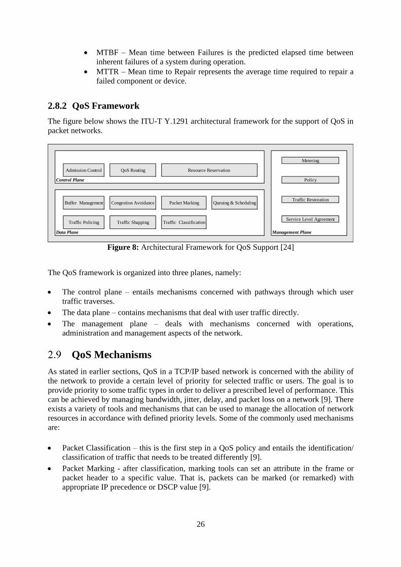
26
• MTBF – Mean time between Failures is the predicted elapsed time between
inherent failures of a system during operation.
• MTTR – Mean time to Repair represents the average time required to repair a
failed component or device.
2.8.2 QoS Framework
The figure below shows the ITU-T Y.1291 architectural framework for the support of QoS in
packet networks.
Figure 8: Architectural Framework for QoS Support [24]
The QoS framework is organized into three planes, namely:
• The control plane – entails mechanisms concerned with pathways through which user
traffic traverses.
• The data plane – contains mechanisms that deal with user traffic directly.
• The management plane – deals with mechanisms concerned with operations,
administration and management aspects of the network.
QoS Mechanisms
As stated in earlier sections, QoS in a TCP/IP based network is concerned with the ability of
the network to provide a certain level of priority for selected traffic or users. The goal is to
provide priority to some traffic types in order to deliver a prescribed level of performance. This
can be achieved by managing bandwidth, jitter, delay, and packet loss on a network [9]. There
exists a variety of tools and mechanisms that can be used to manage the allocation of network
resources in accordance with defined priority levels. Some of the commonly used mechanisms
are:
• Packet Classification – this is the first step in a QoS policy and entails the identification/
classification of traffic that needs to be treated differently [9].
• Packet Marking - after classification, marking tools can set an attribute in the frame or
packet header to a specific value. That is, packets can be marked (or remarked) with
appropriate IP precedence or DSCP value [9].
Control Plane
Data Plane Management Plane
Queuing & Scheduling
Metering
Policy
Traffic Restoration
Service Level Agreement
Resource Reservation QoS RoutingAdmission Control
Buffer Management
Traffic Policing Traffic Shapping Traffic Classification
Congestion Avoidance Packet Marking

27
• Traffic Policing - discarding packets within a traffic stream to restrict the bandwidth
allocated to a class. It ensures that traffic stays within specified limits [9].
• Traffic Shaping – when the data rate of the source is higher than an administratively defined
rate, the excess packets are delayed by holding them in a buffer [9].
• Queuing - refers to the scheduling mechanism used to transmit a packet out of a network
device interface. It defines the order in which packets leave a queue and thus defines the
packet scheduling mechanism. Queuing can also be used to provide fair bandwidth
allocation and minimum bandwidth guarantees [9].
• Congestion Avoidance - Congestion avoidance is complementary to the queuing algorithm.
The queuing algorithm manages the front of a queue, while the congestion avoidance
mechanisms manage the tail end of the queue. Congestion avoidance mechanisms avoid
congestion/bottlenecks through packet dropping [9].
QoS Models
Modern TCP/IP networks are required to transport a variety of traffic types, with varying and
often competing delivery requirements. The IETF has defined three QoS models which are
commonly used in IP networks, namely:
• Best-Effort
• Integrated Services (IntServ) and
• Differentiated Services (DiffServ)
These models have their legacy but are still in-use in provider networks today. In MCC, traffic
from the user to the interfacing gateway, and from the interfacing gateway to the cloud will
traverse an AS that employs one of the aforementioned models. These models are thus studied
next.
2.10.1 Best Effort
This is the default model on IP-based packet networks. It treats all customers and all traffic in
the same way and offers no performance or quality guarantees for any traffic flow [22]. In
MCC, users are no longer satisfied with the best effort service and demand a prescribed QoS.
This model is therefore insufficient to meet the QoS requirements in MCC.
2.10.2 Integrated Services (IntServ)
IntServ is a fine-grain (hard) QoS model and is defined in RFC1633. The model stipulates that
any end-host or application that requires some level of guarantee from the network has to make
an individual reservation before the data transmission occurs. Before transmission is permitted,
admission control is performed by evaluating resource requests against the available resources
[14]. All packets following this flow are treated the same way in every network node along the
path from source to destination. This model has two key features, namely:

28
• Reserved resources – this means each network node is supposed to know what amount of
its resources is already reserved for active flow [14], and
• Call setup – to ensure that end-to-end QoS is met, a flow requiring QoS must first reserve
sufficient resources at each node on the entire path from source to destination path in order
[14].
IntServ uses Resource Reservation Protocol (RSVP) defined in RFC2205 as the underlying
mechanism to signal and explicitly reserve the desired resources for each flow along the end-
to-end path through the network [28]. QoS treatment in MCC requires a combination of
differentiation and prioritization per user and per traffic type. IntServ offers explicit
reservations per user or flow, which is a desirable QoS feature in MCC. IntServ does however
not offer differentiation and prioritization per traffic type, which is also a desirable QoS feature
in MCC. Therefore, IntServ alone will not adequately satisfy the QoS requirement of users in
MCC and will not scale to meet the explosive demand resulting from the number of connections
in MCC.
2.10.3 Differentiated Services (DiffServ)
DiffServ is a coarse-grained QoS model and is defined in RFC2474. In this model, applications
do not need to explicitly request the network to reserve any resources before the data
transmission occurs [29]. Instead, traffic on a network is classified and marked into different
classes - also called Class of Service (CoS). Network nodes (such as routers) are set up to
service multiple classes of traffic with varying QoS requirements. That is,
• On the edge (ingress) of the network or at the boundary of a QoS domain, each packet is
classified into a class by marking the Type of Service (ToS) byte in the IP header using a
Differentiated Services Code Point (DSCP). The DSCP value defines the priority of the
packet [29].
• Along the path from source to destination, specific forwarding treatments are applied by
each network node (using per-hop behaviour (PHB) mechanisms) [29], providing the
packet the appropriate delay-bound, jitter-bound, bandwidth, etc. [30].
DiffServ offers differentiation and prioritization based on traffic classes, which is a desirable
QoS feature in MCC. DiffServ does however not offer explicit differentiation and prioritization
per user or flow, which is a desirable QoS feature in MCC. Therefore, DiffServ alone will not
adequately satisfy the QoS requirement of users in MCC.
The table below summarises the main differences between the three QoS models discussed
above. From the table, IntServ offers a guarantee per flow, while DiffServ offers a guarantee
per traffic class. As stated in the introduction and motivation of this study, users of mobile
devices are longer satisfied with the best effort service and demand QoS when accessing
applications and services hosted in the cloud. To provide end-to-end QoS, MCC services
require both guarantees per user or flow and guaranteed per traffic class.

29
Table 3: Differences between the three QoS models [29]
QoS Service Best Effort IntServ DiffServ
Isolation No
isolation
Per flow isolation Per aggregation isolation
Guarantee No
guarantee
Per flow Per aggregation (Traffic Class)
Service Scope End-to-end End-to-end Per domain
Complexity No setup Per-flow setup Long term setup
Scalability Highly
scalable
Not scalable (each router
maintains per-flow state)
Scalable (edge routers maintain
per aggregate state; core routers
per class state)
Suitable for Real-
Time traffic
No Yes, resource reservation. Yes, Low-latency queuing
(LLQ).
Admission
Control
No Deterministic based on
flows.
Statistic based on Traffic Classes.
Applicability Internet
Default
Small networks and flow
aggregation scenarios.
Networks of any size.
Resource
Reservation
Not
available
Per-flow on each node in
the source-destination
path.
Per Traffic Class on every node
in the domain.
Complexity Low High Medium
As discussed earlier in this chapter, even though resources in MCC are pooled together and
shared amongst multiple clients, the cloud infrastructure is equipped with appropriate metering
capabilities to measure, monitor, track, control, and report usage of these resources on an
individual client basis at some level of abstraction appropriate to the type of service used [14],
[15]. In the next section, monitoring of bandwidth in TCP/IP networks is discussed.
Bandwidth Monitoring
Bandwidth monitoring is a method for measuring the quantity of bandwidth used by network
devices and applications [8]. It involves measuring, collecting and analysing data about flows
in order to gain insight into bandwidth usage, traffic flow, bandwidth hogs and network strain
[30]. Bandwidth usage data can be obtained from target devices and applications using any one
of the following methods:
• Polling or querying data – in this method, a monitoring system is set up to actively obtain
data from a target device or application and refreshes the data collected at a regular interval.
In other words, a “PULL” configuration. Typical examples include HTTP requests, HTTPS
requests, port checks, email checks, FTP downloads, and database requests [8].
• Listening or receiving data - in this method, a monitoring system is set up to passively
obtain data from a target device or application. That is, the data is automatically pushed
from the target device or application to the monitoring system. In other words, a “PUSH”

30
configuration. Common examples include SNMP traps, Syslogs, xFlow, and event log
messages [8].
Nowadays, the exponential growth in mobile broadband data traffic is resulting in increased
pressure on already limited network resources. Therefore, without a comprehensive insight into
network traffic, it would be virtually impossible to ensure the proper availability of mission-
critical services and applications. By monitoring bandwidth usage and applying appropriate
QoS policies, administrators are able to ensure that users with a prescribed level of QoS get
priority and are guaranteed minimum bandwidth. Information regarding traffic flow on a
TCP/IP based network can be captured and analysed for a target device or application using
one of the approaches discussed below:
• Packet Analysis - Packet analysis uses packet capturing technologies such as Switched Port
Analyzer (SPAN), Remote Switched Port Analyzer (RSPAN), or Encapsulated Remote
Switched Port Analyzer (ERSPAN) to copy packets from specific interfaces. Full packet
header and payload are collected and analysed [31].
• Flow Analysis - In contrast to packet analysis, flow analysis does not make a copy of the
full packet header and payload but instead collect metadata such as traffic protocol, website
names, top talkers, top connections, bandwidth usage, from network traffic and send the
metadata to a flow collector as UDP packets [31].
Bandwidth usage data on a TCP/IP network can be obtained from target devices and
applications using the following data acquisition methods [30].
• SNMP
• xFlow (such as NetFlow, IPFIX, sFlow, jFlow, etc), and
• Packet Sniffing
SNMP is an application layer protocol defined in RFC1157 and is used to facilitate the
exchange of management information between network devices such as servers, routers, hubs,
and switches as well as end points like printers, scanners, and IOT devices. Its most recent
iteration is version 3. SNMP data provides useful information regarding bandwidth usage on a
port-by-port basis but has its limitations as it does not differentiate traffic by type of service or
protocol type. From an implementation perspective, SNMP needs to be supported and enabled
on the target device, and devices require the same configuration such as the SNMP version and
SNMP community string, which may not be practical in MCC where different ASs are involved.
Differentiating traffic by type of service or protocol type is essential in MCC, packet sniffing
is considered as the preferred mechanism to obtain bandwidth usage data in this study and is
discussed next.
Packet Sniffing
Packet sniffing is the process of capturing incoming or outgoing packets transmitted over a NIC
and analysing its content. Packet sniffing is implemented using a functional entity called a
packet sniffer. A packet sniffer is a piece of software or hardware that is used to capture and
copy incoming or outgoing packets on a network where the sniffer is installed or attached to.

31
Sniffers available in both software and hardware variants and comes with features that allow
them to log, analyse and decode the contents and bandwidth usage information of captured
traffic. Software sniffers are available in both commercial and freeware variations and offer
greater convenience compared to their hardware counterparts. However, their performance is
largely influenced by factors such as [9]:
• Operating System in use,
• Hardware supported,
• Memory size,
• CPU speed, and
• Disk I/O and memory bandwidth.
Therefore, to monitor and analyse large networks, or networks with bit rates above 10 Gbps,
hardware sniffers are often preferred. This is because components of hardware sniffers such as
network adapters, memory/disk bandwidth, and buffer management are purely optimized for
the monitoring and analysis job and will thus yield better performance [9]. In addition to real-
time analysis, data captured by the sniffer can be stored in a database for offline analysis.
Compared to freeware, commercial packet sniffers generally offer much more sophisticated
analysis tools, more user-friendly interfaces, and support a wider variety of wired and wireless
media [30].
Packet sniffers predominantly operate as passive sniffers and only collect copies of packets sent
or received by applications and protocols on the network and do not send packets themselves
[9]. The data captured by the packet sniffer can be analysed and decoded for various useful
purposes and benefits such as:
• Network troubleshooting,
• Communication protocol analysis,
• Network traffic analysis,
• Traffic trend and predictive analysis,
• Monitor bandwidth usage,
• Identify bottlenecks, and
• QoS monitoring,
Packet Sniffer Structure
As stated in the preceding, a packet sniffer captures copies of packets sent to or received from
a network device. It comprises various components as discussed below:
• Hardware – most packet sniffers work from standard network adapters (wired or wireless).
However, some sniffers may require specialized hardware [10].
• Capture Library – this component is responsible for capturing a copy of every link-layer
frame sent or received by a network device, filters it for specified traffic, and then stores

32
the data in a buffer [10]. The actual collection can be done using pcap (in Linux based
systems) or libcap (in Window-based systems).
• Buffer – this component is used to store copies of packets captured. The buffer can be used
to store packets until the buffer fills up, or in a round-robin fashion where the newest data
replaces the oldest data [10].
• Bandwidth Analyzer – this component is used for traffic analysis [10].
• Decode – this component displays the content of network traffic with the descriptive text
[10].
Figure 9 below shows the basic structure of a packet sniffer.
Figure 9: Structure of a Packet Sniffer [32].
On the right of the above figure are the (Internet) protocols used for providing user services
(such as HTTP, HTTPS, FTP, Telnet, SNMP, DHCP, and so on) as well as the applications
(such as web browsing or FTP client) that ordinarily run on a user computer.
Most packet sniffers can be configured to operate in one of the two ways discussed below:
• Unfiltered – meaning the sniffer will capture all possible packets [10].
• Filtered – meaning the sniffer will only capture packets that contain specific data elements
[10].
Most packet sniffers work as a pcap application. Figure 10 below shows the typical flow of a
pcap application.
Application
Operating
System Transport Layer (TCP/UDP)
Network Layer (IP)
Link Layer (Ethernet)
Physical Layer
to/from network to/from network
Packet
Analyzer
Packet
Capture
(pcap)
Application (e.g., www
browser, ftp client)
Packet Sniffer
copy of all frames
sent/received

33
Figure 10: Standard PCAP Application Flow [32].
As per the above figure,
• The first step in a pcap application is to initialize the network interface and open a session,
then set the filter to filter the packets to be accepted or rejected [9].
• Packets are then accepted, and a log is continuously maintained until the interface is closed,
and the session is ended [9].
As the packet travels from source to destination in a TCP/IP network, each layer of the Open
System Interconnect (OSI) model adds its own header information as illustrated in Figure 11
below.
Figure 11: Data Encapsulation in a TCP/IP Network [32].
Capture Loop
Initialize Network
InterfaceCapture Packet
Process Packet
Set Filter
Close InterfaceExit
5 - 6 - 7 - Application
User Data (Messages or Stream)
4 - Transport
3 - Network
2 - Data Link
Network-Specific frames
14 4
1 - Physical
Transport Protocol Messages
IP Datagram
Telnet, FTP, TFTP,
DHCP, SNMP,
TCP, UDP
IP, ARP, ICMP
PPP, Ethernet
Physical Devices
Ethernet
Trailer
Ethernet
HeaderIP Header TCP Header Application Data
20 20 …....
User Data
User dataApp
Header
Application DataTCP Header
IP Header TCP Header Application Data
TCP Segment
IP Datagram
46 to 1500 bytes
Ethernet Frame

34
Starting at Layer 1, the first header is an Ethernet header, followed by an IP header, then the
TCP header, and finally the Application Data. At the Network Layer, a trailer is also added.
Each header contains vital information that can be analysed by a packet sniffer to provide some
useful information about the intent of the communication.
The Ethernet is built around a “shared principle”. That is, all computers on a local network or
local network segment can “see” all the traffic on the same wire. Each host on the shared wire
is assigned a unique identifier called a MAC address. The Ethernet NIC is built with a “filter”
that ignores and discards all traffic whose MAC address does not match the MAC address of
its own Ethernet network adapter [10]. Therefore, to capture all packets, the Ethernet Network
Interface Card will be placed in what is called a “promiscuous mode” [8]. This removes the
“filter” limitation on the Ethernet Network Interface Card, thereby enabling it to pick up all
network traffic.
2.13.1 Packet Header-based Sniffing
In MCC, Ethernet is used as a layer 2 transport technology, while IP is used as a Layer 3
transport protocol. Figure 12 below depicts the structure of an Ethernet header.
Figure 12: Ethernet Packet Structure [29].
According to Figure 12, the Ethernet header contains a 2 or 6-Bytes Source (MAC) Address
field and a 2 or 6-Bytes Destination (MAC) Address field. By capturing and analyzing the
content of these fields, the packet sniffer is able to determine the source device and the
destination device. The Payload field is where the actual data that needs to be transmitted is
inserted. Based on the layer 2 Ethernet packet header information, a packet sniffer can be setup
to report on bandwidth usage according to a specific Source (MAC) Address, or Destination
(MAC) Address, as at layer 2, no Protocol or Type of Service information is visible.
To transport Ethernet packets in a TCP/IP network, and MCC alike, the Ethernet packets are
encapsulated into IP Datagrams by appending a TCP and IP header. In what follows, the
structure of the IPV4 and IPV6 headers are discussed in order to understand the different types
of information that can be accessed by a packet sniffer within an IPV4 and IPV6 Datagram.
Figure 13: IPV4 Packet Header Structure [29].
Bytes 7 1 2 or 6 2 or 6 2 0 to 1500 0 to 46 4
PreambleStart-Frame
Delimiter
Destination
Address
Source
Address
Type of
LengthData Pad Checksum
0 1 2 3 4 5 6 7 8 9 10 11 12 13 14 15 16 17 18 19 20 21 22 23 24 25 26 27 28 29 30 31
0 1 2 3 4 5 6 7 8 9 10 11 12 13 14 15 16 17 18 19 20 21 22 23 24 25 26 27 28 29 30 31
Options Padding
Version Length ToS/DSCP/ECN Total Length
Identification Flags Fragment Offset
Time to Live Protocol Header Checksum
Source Address
Destination Address

35
As defined in RFC 791, the IPV4 packet header length is variable and is defined in the Internet
Header Length field. Whereas the total length of the IPV4 datagram (include header and data)
is defined in the Total Length Field. The header contains vital information needed for routing
and delivery. The packet sniffer can examine the header and determine essential information
about the flow, such as:
• TOS/ DSCP – indicate the traffic class of each packet.
• Protocol – indicate the protocol used for communication (TCP or UDP).
• Source Address – indicates from which device the packet is sent.
• Destination Address – indicate to which device the packet is sent.
Port numbers identify which program the packets need to be directed to on the remote device.
It also identifies the session on the local device. It worth noting that some applications can be
detected by simply identifying the port over which communication takes place, such as port 80
for HTTP. However, some applications can hide their identity in the payload itself, and deep
packet inspection may be required to search for the application signature.
To deal with the problem of IPV4 addresses exhaustion, the IETF developed the Internet
Protocol version 6 (IPV6). Figure 14 below depicts the structure of an IPV6 packet header.
Figure 14: IPV6 Packet Header Structure [29].
As defined in RFC 2460, the IPV6 packet header also has a variable length. The packet sniffer
can examine the header and determine essential information about the flow, such as:
• Traffic Class – indicate the traffic class for the packet.
• Source Address – indicates from which device the packet is sent.
• Destination Address – indicate to which device the packet is sent to.
The IPV6 header is much simpler and easier to process than the IPV4 header. Unlike the IPV4
header which contains a Protocol field, the IPV6 header does not contain a Protocol field. IPv4
has the ability to identify the type of service field and specify QoS requirements on precedence,
delay, throughput and reliability. In a similar manner, IPv6 has a differentiated service code
point field and can support QoS per flow on the network layer (e.g., by using flow label and
next header options). Both IPv4 and IPv6 do not guarantee the actual end-to-end QoS as there
is no reservation of network resources, and QoS guarantee needs to be provided by other
mechanisms in the IP network [24]
0 1 2 3 4 5 6 7 8 9 10 11 12 13 14 15 16 17 18 19 20 21 22 23 24 25 26 27 28 29 30 31
0 1 2 3 4 5 6 7 8 9 10 11 12 13 14 15 16 17 18 19 20 21 22 23 24 25 26 27 28 29 30 31
Hop Limit
Destination Address
Source Address
Version
Payload Length
Traffic Class Flow Label
Next Header

36
In Mobile IP and MCC alike, due to the mobility of users, each device is assigned two unique
IP addresses. One IP address is used for routing and the other IP address is used as a session
identifier. In addition, the International Mobile Subscriber Identify (IMSI) and Mobile Station
International Subscriber Directory Number (MSISDN) are used to uniquely identify the
subscriber on a network.
• The IMSI is stored in the Subscriber Identity Module (SIM) card and does not change.
• The MSISDN is the number normally dialled to connect a call to the mobile device and
can change in time.
The packet sniffer can copy and inspect the information contained in each header to reveal the
communication intent.
Bandwidth Control
Bandwidth control is an essential aspect of QoS enforcement and refers to the different types
of actions that can be applied to a traffic flow [9]. It entails applying techniques to dynamically
limit and customize the distribution and consumption of bandwidth by devices and applications.
Bandwidth control can be achieved by applying the QoS policies discussed below:
• Policing – traffic policing allows an administrator to define a maximum rate at which traffic
can be sent (upload) or received (download) at an interface of a device. When the data rate
of the source is higher than expected, the excess traffic is dropped (or remarked) [9].
• Shaping – shaping is less extreme than policing. When the data rate of the source is higher
than expected, the excess traffic is retained in a buffer or queuing mechanism for later
transmission [9].
• Priority queuing – queuing defines the order in which packets leave a queue (packet
scheduling mechanism) and is intended to accommodate temporal congestion on a network
device’s interface. Queuing allocate bandwidth to prioritized applications before allocating
to other applications. This ensures that priority traffic is always transmitted ahead of other
traffic, while excess packets are stored in buffers until bandwidth becomes available [9].
An action is chosen that best fits the QoS requirements of the user or application. For instance,
a scheduling and queuing mechanism can be selected that allows a network node to allocate
more bandwidth to one user or application by transmitting more of the user's traffic. This means
that packets for a user or application that is given bandwidth priority are scheduled for
transmission more regularly than other packets. Congestion occurs when packets enter a device
faster than they can exit.
For allocating bandwidth, some of the most commonly used queuing and scheduling
mechanisms for congestion management are [9].
• RED (Random Early Detection)
• W-RED (Weighted Random Early Detection)
• WFQ (Weighted Fair Queuing)

37
• CBQ (Class-Based Queuing)
• CB-WFQ (Class-Based Weighted Queuing)
• CQ (Custom Queuing)
• PQ (Priority Queuing)
• FIFO (First-In-First-Out)
• FCFS (First-Come, First Served)
• LLQ (Low Latency Queuing)
The study of the features and functions of these queuing and scheduling mechanisms is outside
the scope of this work. It is, however, worth noting that RSVP can be used in conjunction with
CBWFQ. Moreover, mechanisms such as WRED, LLQ or CBWFQ can be enabled at the same
time [9].
Quality of Service Monitoring
As discussed in earlier sections, QoS defines a set of techniques that are used to manage and
optimize the allocation and utilization of network resources. QoS in a network can be actively
or passively measured in order to obtain values for the following parameters for each
communication:
• Delay,
• Jitter,
• Packet Loss, and
• Bandwidth.
As stated in earlier sections, the fundamental QoS mechanisms are;
• Marking,
• Classification,
• Shaping,
• Policing, and
• Queuing.
To implement QoS, the interfacing gateway needs to support these fundamental QoS
mechanisms. Without QoS policies in place, IP network links function on a best-effort delivery
basis, where all traffic has equal priority, and traffic packets for all applications, users or
services have an equal chance of being delivered. When the network becomes congested, all
packets have an equal chance of being dropped. With policies in place, an administrator can
configure network nodes to provide the required priority treatment to a specific application or
user traffic, before distributing to others.
When a packet sniffer is installed in any of the nodes or as any of the nodes on a network, it
captures packets passing through the local node’s interface(s), irrespective of the source or
destination of the packets. This is fine if the interest is only to monitor the traffic of this node.
In switched networks, only traffic for a specific node is sent to each node’s network card.
Therefore, the sniffer usually cannot discern the traffic of other machines in the network.
Therefore, if the interest is also to monitor the traffic of other devices in the network or in the

38
case of network-wide monitoring, a switch that offers a monitoring port or port mirroring
configuration should be used. In this case, the switch sends a copy of all packets travelling
through the switch to the monitoring port. The sniffer is then connected to the monitoring port
to extract and analyse all the data that passes through the switch, or alternatively, the sniffer
can be set up as the gateway for all devices in the network [8]. The latter option is considered
for this study where the packet sniffer is installed on the gateway connecting the mobile devices
to the cloud in order to provide network-wide monitoring.
Review of Previous Related Studies:
Over the past few years, MCC has been advancing the landscape of MC by providing on-
demand, measured, elastic, self-service, and broad access services to mobile users using IaaS,
PaaS, and SaaS delivery models. Although MCC offers several benefits, a number of challenges
such as security, privacy, service availability, QoS guarantee, low bandwidth, network
management, heterogeneity, and pricing problems, have constrained the adoption of MCC.
Several MCC research architectures have been proposed over the past seven years. Out of the
30 architectures surveyed by [33], the majority are based on a layered approach with
components such as mobile users, network operators, Internet Service Providers, Application
Service Providers, and Data Centre owners. An architecture consisting of interfacing has mostly
been used in studies that investigate the problem of bandwidth allocation and bandwidth pricing
in MCC. [34] conducted an investigation into the problem of bandwidth shifting and
redistribution resulting from the varying bandwidth demands of gateways as a result of the
mobility of mobile users. They addressed the problem of QoS-guaranteed bandwidth shifting
and redistribution among a pool of cooperating gateways by formulating bandwidth
redistribution as a utility maximization problem and solved it using a modified descending bid
auction in a scheme called AQUM (Auction based Quality of service guaranteed Utility
Maximization). In the scheme, each gateway aggregates the demand of connected mobile
devices and makes a bid for the required amount of bandwidth from the CSP.
[35] also studied the problem of QoS-guaranteed bandwidth shifting and redistribution among
interfacing gateways in MCC. They also considered a descending price bid auction using the
AQUM scheme and worked out the theoretical maximum and minimum selling price of
bandwidth and proved the convergence of AQUM. [36] also investigated the problem of QoS-
guaranteed bandwidth shifting and redistribution in MCC using AQUM, but formulated service
delay as the utility maximization problem. They modelled the utility of the interfacing gateways
using revenue and cost functions and analysed the Nash Equilibrium, and derived the theoretical
maximum and minimum selling prices of bandwidth and proved the convergence of AQUM.
[37] also looked into the problem of bandwidth shifting and redistribution in MCC. They
formulated bandwidth redistribution as a utility maximization problem and solve it using a
modified descending bid auction in a scheme called AAQUM (Advanced Auction based QoS
ensured Utility Maximization). In their proposed scheme, each interfacing gateway aggregates
the bandwidth demand of connected mobile devices and submits its bandwidth bid to the
auctioneer cum CSP. During the auction process, the CSP distributes the bandwidth among the
gateway, maximizing its profit and ensuring QoS to mobile devices.

39
[38] also investigated the problem of QoS-guaranteed bandwidth allocation and instead of
focussing on utility maximization alone, they also considered revenue maximization. They
extended AAQUM into a scheme called AQUMR (Auction based Quality of service guaranteed
Utility Maximization and Revenue Maximization). Similar to AQUM, each interface gateway
sums the demands of connected mobile devices and submits a bid for the required amount of
bandwidth from the CSP. In the scheme, each gateway seeks to maximize its revenue and
competition is introduced between gateways by setting the demand at different ranges using
fuzzy auctioning. With each iteration of the auction process, the price per unit is decreased
based on the demand for bandwidth at the gateway.
These studies have primarily focussed on solving the bandwidth pricing problem in MCC.
Whereas the investigation in this study also looks into the problem of bandwidth allocation and
QoS in MCC and proposed to use interfacing gateways as discussed further in the next chapter.

40
Chapter 3
3 System Model
Introduction
In this study, the problem of packet sniffing and bandwidth redistribution in MCC is
investigated. Specifically, data regarding bandwidth usage per user, device and application is
measured, monitored, and tracked using a packet sniffer, while bandwidth guarantee to devices
accessing services hosted in the cloud is enforced using a dynamical bandwidth management
algorithm that redistributes bandwidth among a pool of cooperating gateways as users roam
around and change their link-layer connection from one gateway to another. In what follows,
the MCC system model is considered, and the mathematical modelling of the proposed
algorithm is presented.
MCC System Model
By and large, providing end-to-end QoS in IP-based networks is difficult due to their hetero-
geneity. As discussed in earlier sections, services in MCC are hosted in the cloud are accessed
via the Internet. A number of MCC architectural models have been proposed over the years.
This study considers the MCC model as shown in Figure 15 below.
G1G2 GL
CSP
U11 U1N U21 U2N UL1 ULN
AS-1 AS-2 AS-LSLA SLA
User Device Layer
CSP Layer
Radio Access Layer
ISP Layer
Figure 15: MCC Model.
The model consists of three network domains (AS-1, AS-2, and AS-3), and a CSP. Each AS is
represented as a cloud. Each domain has an interfacing gateway that connects users to the CSP
via the public Internet using high-capacity fixed communication links. In total, there are 𝑙 interface gateways. The interface gateways is a functional element proposed to be implemented
in a selected network node to provide QoS within a network domain. It is part of the control
plane and communicates with the users, CSPs, and with interfacing gateways of adjacent
domains (inter-domain). Connecting with adjacent gateways may require direct communication

41
between the gateways. Its control plane performs functions such as admission control, QoS
routing, and resource reservation, while its Data plane performs functions such as traffic
classification, packet marking, traffic shaping, traffic policing, buffer management, queuing,
and scheduling. Whereas its management plane performs functions such as metering, policy,
and SLA. It controls bandwidth allocation within a domain by accepting or rejecting requests
for the QoS service using the admission control function.
• A mobile user requests a QoS service (in this case, an amount of bandwidth) from the
gateway to which it connects. This can be achieved using RSVP.
• The gateway receives the request and aggregates the demand for connected devices and
requests for the required amount of bandwidth from the CSP. This can be achieved using
RSVP.
As a mobile user moves from one location to another, the gateway that connects the user to the
CSP may change. Consequently, the aggregate demand of the gateways may also change as
devices may be detached, or new devices may be attached. A mobile user may be able to access
a web application or cloud service at one location but may find it difficult to access the same
application or cloud service at another location. This could be due to insufficient bandwidth on
the new gateway, or for not shifting bandwidth that was allocated to the mobile user from the
gateway where it was previously connected to the gateway where it is located. Resource
management in each domain is accomplished using the DiffServ architecture, due to its
scalability.
The gateways are represented by the set:
𝐺 = {𝐺1, 𝐺2, …… . 𝐺𝐿} (2)
From the above, the number of gateways is variable. However, due to memory and processing
limitations on the host computer, the number of virtual hosts that can be instantiated
simultaneously is limited. In the virtual network lab, 𝐿 = 2 is used. However, the number of
gateways is increased in the Matlab algorithm.
At a timeslot 𝑡, each gateway has 𝑛 mobile devices connected via a wireless Radio Access
Network. Each device has its unique bandwidth requirement. Each mobile device requests the
required amount of bandwidth 𝑤𝑛(𝑡), for (1 ≤ 𝑛 ≤ 𝑁) from the gateway to which it is
connected. Each gateway aggregates the demand of all connected mobile devices and requests
the required amount of bandwidth from the CSP. For each gateway, this aggregate 𝐺𝑖(𝑡) is
represented by the equation:
𝐺𝑖(𝑡) = ∑ 𝑤𝑛(𝑡)𝑁𝑛=1 . (3)
In terms of the metering feature, which is part of the management plane, a usage-based billing
model is typically considered. In this model, the CSP earns revenue from serving the connected
gateways with bandwidth and QoS services. Each gateway also earns revenue from serving the
connected devices with bandwidth and QoS services and incurs costs to pay for the bandwidth
and QoS services allocated by the CSP. To be profitable, the gateway seeks to serve the users
profitably. Several previous studies [36], [39], [40], [41] have considered an auction-based
algorithm to distribute and shift bandwidth. However, as stated in Chapter, auction-based
bandwidth shifting and redistribution are beyond the scope of this study.

42
The total available bandwidth at the CSP is denoted by 𝑄 and is a constraint of the network.
That is:
∑ 𝐺𝑖(𝑡)𝐿
𝑖=1 ≤ 𝑄. (4)
𝑓𝑜𝑟 (1 ≤ 𝑖 ≤ 𝐿)
This means that the total bandwidth demands of the gateways should be less than or equal to
the available CSP bandwidth. If the aggregate demand of the gateways is more than the
available CSP bandwidth, congestions occur. This will result in service degradation, and a
policy and a queuing mechanism are required to define the order in which packets from the
different gateways are buffered (in the case of traffic shaping) while waiting for transmission,
or the order in which packets from the different discarded are discarded (in the case of traffic
policing).
Each gateway may also require some reserve bandwidth β from the CSP for its internal
operations.
𝐺𝑖(𝑡) + β𝑖(𝑡) (5)
𝑓𝑜𝑟 (1 ≤ 𝑖 ≤ 𝐿)
For the model considered in this study, this bandwidth can be added to the aggregate bandwidth
demand of each gateway. That is;
∑ 𝐺𝑖(𝑡)𝐿
𝑖=1 + ∑ β𝑖(𝑡)
𝐿
𝑖=1 ≤ 𝑄. (6)
Therefore, the demand requested by the gateway from the CSP is the sum of the aggregate
demand of the connected devices plus the bandwidth required for the gateway’s internal
operations.
Service Delay
As stated in the previous section, at a timeslot 𝑡, there are 𝑛 mobile devices connected to each
gateway (1 ≤ 𝑛 ≤ 𝐿). A packet will take some amount of time to travel between the mobile
device and the gateway, and similarly, between the gateway and the CSP. Depending on the
location of the Data Centre hosting the CSP services, traffic from a mobile device may need to
traverse several domains before reaching the Data Centre in question.
In a digital communication system, as stated in Chapter 2, delay refers to the time taken by a
packet to move from a point on the network to another, such as from (its) source to (its)
destination. Assume 𝑇𝑖𝑛 to be the transmission delay required by the mobile user 𝑛𝑖 to access a
service 𝑖. If the total available bandwidth 𝑄 is completely allocated to the gateway 𝐺𝑖 , then the
total transmission delay for the gateway is given by [36], [19]:
𝑇𝑖 = ∑ 𝑇𝑖𝑛|𝑛𝑖|𝑛=1 (7)
where
• | | indicates the cardinality of the set.

43
As stated in the foregoing, the bandwidth requested by each gateway from the CSP is denoted
by 𝐺𝑖(𝑡)), which is determined by the aggregate bandwidth required to meet the QoS needs of
connected mobile devices and the amount of bandwidth required to meet the gateway’s own
operation (denoted by 𝛽). The total bandwidth demand requested by the gateway from the CSP
is given by:
∑ 𝐺𝑖(𝑡) + ∑ 𝛽𝑖(𝑡)
|𝑛𝑖|
𝑛=1
|𝑛𝑖|
𝑛=1
(8)
However, in this study, the value of 𝛽𝑖(𝑡) is negligible and is not considered in the calculations.
As stated in earlier sections, QoS in MCC is observed by measuring performance matrices such
as packet loss, and delay. Therefore, by monitoring the time taken by a packet as captured by
the packet sniffer, appropriate QoS policy and scheduling mechanisms can be applied to ensure
that the delay remains within the prescribed thresholds. For TCP communications, an ACK
packet is sent for every packet received, confirming the delivery of the packet. Therefore, the
Round-Trip Time (RTT) for ACK packets can be measured by a packet sniffer and can be used
to gauge service delay in MCC. For the UDP packet, there is no ACK packet and delay cannot
be measured with the packet sniffer and needs other utilities to be added to the interfacing
gateway.
Packet Sniffing
In this study, a passive packet sniffer deployed on the interface gateway is used to measure,
monitor and track bandwidth used by individual devices. Using a packet sniffer to collect
bandwidth usage information offers much more granular details compared to traditional
mechanisms like using SNMP. The packet sniffer is an added function on the interface gateway
and works in coordination with the data plane, control plane and management plane of the
gateway to ensure bandwidth allocation and QoS.
Bandwidth Redistribution
In the MCC context, the bandwidth redistribution problem differs from the traditional
bandwidth allocation problem in the sense that traditional bandwidth allocation is concerned
with allocating proportional bandwidth to all gateways, even if only a few gateways change
their demand. Whereas bandwidth redistribution is concerned with allocating bandwidth to the
specific gateway that has changed its bandwidth demand [42]. The redistribution of bandwidth
is necessary to satisfy bandwidth and QoS guarantees to mobile devices.
Each wireless channel connecting a mobile device to a gateway has a different spectral
efficiency, which can be represented by the set:
𝐸(𝑡) = {𝐸1(𝑡), 𝐸2(𝑡)…… . 𝐸𝑁(𝑡)}. (9)
The channel spectral efficiency is measured in bits/s/Hz and defines the maximum information
rate that can be transmitted over a given bandwidth in a particular communication system. It is
obtained using the Shannon Equation, which is [1]:
𝐶 = 𝜔 ∙ 𝑛 ∙ log2(1 + 𝑆𝑁𝑅) (10)

44
where:
• 𝐶 is the channel capacity,
• 𝜔 is the spectrum,
• 𝑛 is the number of antennas, and
• 𝑆𝑁𝑅 is the Signal to Noise Ratio.
Due to the different spectral efficiencies, each gateway utilizes a percentage of the bandwidth
allocated by the CSP [36], [19]. As devices roam from one location to another, it may, therefore,
occur that some gateways can become overloaded, while others may be underutilized. As stated
in Chapter 1, an investigation into QoS guarantee in the Wireless Access Network is beyond
the scope of this study.
Dynamical Bandwidth Allocation Algorithm
The study considers a system model where mobile devices connect to the CSP via the gateways,
as depicted in Figure 16 below.
Figure 16: Simulation Model Before U2 Movement.
As opposed to requesting bandwidth directly from the CSP, the mobile devices signal their
request for bandwidth to the gateway to which they connect. The gateway subsequently
aggregates the demand of the connected devices and requests the required amount of bandwidth
from the CSP. The QoS service is measured in terms of the service delay, as represented in
equation (7). As devices move from one location to another as depicted in Figure 17 below, the
aggregate bandwidth demand of the gateways may vary.
CSP
G1
U1 U2
G2
U3 U4

45
Figure 17: Simulation Model After U2 Movement.
Due to the movement of users, an algorithm is required to achieve the following objectives:
• To dynamically redistribute the bandwidth from the cloud to the gateways, and
• To dynamically allocate the bandwidth from the gateways to the mobile devices.
In what follows next, the algorithm investigated in this study is discussed.
In the algorithm, bandwidth is allocated to the gateways based on the aggregate demand of the
connected users, and in cases of contention, the proportional method is used to determine the
allocation. This means that the gateways with bigger demand are allocated more bandwidth,
whereas gateways with smaller demand are allocated lesser bandwidth.
1) Start (initialization).
2) CSP broadcast maximum bandwidth available (𝑄) to connected gateways.
3) Each gateway broadcast maximum bandwidth available (𝑄) to connected devices.
4) Connected device sends their bandwidth request (𝑤𝑛) to the corresponding gateway.
• In the simplified model considered, there are in total 2 gateway (𝐿 = 2) connected
to the CSP. Each gateway has 2 devices connected (𝑁 = 2). For instance,
for gateway 1, 𝐺1 = [𝑑11 𝑑12] and
gateway 2, 𝐺2 = [𝑑21 𝑑22]
(11)
• 𝑑1𝑗 is the jth device connected to the gateway 𝐺1.
• 𝑑2𝑗 is the jth device connected to the gateway 𝐺2.
• The bandwidth demand of the devices is arranged into a 2 x 2 matrix with the
elements of each gateway arranged along the rows of the matrix.
𝑤 = [
𝑑11 𝑑12
𝑑21 𝑑22]
(12)
5) Each gateway aggregates the demand for connected devices and submits its bandwidth
demand to the CSP.
CSP
G1
U1
G2
U3 U4 U2

46
𝐺𝑖_𝑎𝑔𝑔(𝑡) = ∑ 𝑤𝑛(𝑡)𝑁𝑛=1 (13)
for 1 ≤ 𝑖_𝑎𝑔𝑔 ≤ 𝐿
• The aggregate per gateway is performed by adding up the elements along the rows
in the L x N matrix produced in 3) above. That is, a summation is performed along
each row. For instance:
𝐺1_𝑎𝑔𝑔 = [𝑑11 + 𝑑12] and
𝐺2_𝑎𝑔𝑔 = [𝑑21 + 𝑑22]
(14)
• The result is arranged into a 2 x 1 matrix, with the aggregate bandwidth demand of
each gateway arranged along the rows of the matrix.
𝐺𝑖_𝑎𝑔𝑔
(𝑡) = [𝐺1_𝑎𝑔𝑔(𝑡)
𝐺2_𝑎𝑔𝑔(𝑡)]
(15)
6) After receiving all the gateway demands, the CSP aggregates the requests.
𝐶𝑆𝑃𝑎𝑔𝑔(𝑡) = ∑ 𝐺𝑖_𝑎𝑔𝑔(𝑡)
𝑛
𝑖=1 ≤ 𝑄.
(16)
• This aggregate is obtained by summing up the values along the column of the 2 x 1
(L x 1) matrix obtained in (4) above. This produces a scalar quantity, which
represents the total amount of bandwidth requested by all gateways (and by
extension, the total bandwidth demand of all connected mobile devices).
• The aggregate 𝐶𝑆𝑃𝑎𝑔𝑔(𝑡) should preferably be less than or equal to the total
bandwidth available at the CSP (𝑄). If more than 𝑄, congestion occurs.
7) CSP proportionally allocates the bandwidth to the gateways.
𝐺𝑖_𝑟𝑎𝑡𝑒(𝑡) =
𝐺𝑖_𝑎𝑔𝑔(𝑡)
𝐶𝑆𝑃𝑎𝑔𝑔(𝑡)
(17)
• The result of this calculation is a 2 x 1 matrix, with the bandwidth allocated to each
gateway appearing as the row elements of the matrix.
𝐺𝑖_𝑟𝑎𝑡𝑒(𝑡) = [
𝐺1_𝑟𝑎𝑡𝑒
𝐺2_𝑟𝑎𝑡𝑒]
(18)
• Due to the spectral efficiency (𝐸𝑖(𝑡)) of the channel connecting each gateway to the
gateway, each gateway (𝐺𝑖) only utilizes a percentage of the bandwidth allocated by
the cloud as denoted by the formula below:
𝐺𝑖_𝑒𝑟𝑎𝑡𝑒(𝑡) = 𝐺𝑖_𝑟𝑎𝑡𝑒(𝑡).∗ 𝐸𝑖(𝑡) (19)
• Therefore, the effective aggregate bandwidth used by all gateways connected will
be less than the aggregate bandwidth allocated to the gateways by the cloud.

47
∑ 𝐺𝑖_𝑒𝑟𝑎𝑡𝑒𝐿
𝑖=1(𝑡) ≤ ∑ 𝐺𝑖_𝑟𝑎𝑡𝑒
𝐿
𝑖=1(𝑡) (20)
8) The gateways receive the bandwidth allocated by the CSP and proportionally allocates
it to the connected devices.
𝐷𝑛𝑟𝑎𝑡𝑒
(𝑡) =𝑤𝑛(𝑡)
𝐺𝑖𝑎𝑔𝑔
.∗ 𝐺𝑖𝑟𝑎𝑡𝑒(𝑡)
(21)
• The result of this calculation is a 2 x 2 matrix, with the bandwidth allocated to each
device arranged along the rows of the matrix.
[𝑑11𝑟𝑎𝑡𝑒
(𝑡) 𝑑12_𝑟𝑎𝑡𝑒(𝑡)
𝑑21𝑟𝑎𝑡𝑒(𝑡) 𝑑21_𝑟𝑎𝑡𝑒(𝑡)
] (22)
• 𝐷𝑖𝑗_𝑟𝑎𝑡𝑒 is the bandwidth allocated by the device 𝑗 connected to gateway 𝑖.
• Due to the spectral efficiency (𝐸𝑛(𝑡)) of the wireless channel connecting each
device to the gateway, each device (𝐷𝑛) only utilizes a percentage of the bandwidth
allocated by the gateway as denoted by the formula below:
𝐷𝑛_𝑒𝑟𝑎𝑡𝑒(𝑡) = 𝐷𝑛_𝑟𝑎𝑡𝑒(𝑡).∗ 𝐸𝑛(𝑡) (23)
• Therefore, the effective aggregate bandwidth used by all devices connected to a
gateway will be less than the aggregate bandwidth allocated to the devices by the
gateway.
∑ 𝐷𝑛_𝑒𝑟𝑎𝑡𝑒(𝑡)
𝑁
𝑛=1 ≤ ∑ 𝐷𝑛𝑟𝑎𝑡𝑒
(𝑡)𝑁
𝑛=1
(24)
9) End if
The algorithm above is further set out in the flow chart and transmission diagram below.
Figure 18: Algorithm Transmission Diagram
GatewayMobile Device CSP
CSP broadcast available bandwidth
Device send request to the Gateway
Gateway send request to the CSP
CSP allocate bandwidth to Gateways
Gateway broadcast available bandwidth
Gateway allocate bandwidth to Devices
1
5
4
6
3
2

48
Figure 19: Algorithm Flow Chart
For the gateways to cooperate, a communication relationship needs to exist between them
directly or via a central control system.
From the particular case investigated above, the general mathematical model below can be used
to allocate bandwidth dynamically when there are more gateways (𝐿) and mobile users (𝑁)
connected to the cloud.
Each gateway aggregates the demand for connected devices and submits its bandwidth demand
to the CSP:
𝐺𝑖_𝑎𝑔𝑔(𝑡) = ∑ 𝑤𝑛(𝑡)𝑁𝑛=1 (25)
for 1 ≤ 𝑖_𝑎𝑔𝑔 ≤ 𝐿
The aggregate per gateway results in an L x 1 matrix, with the aggregate bandwidth demand of
each gateway arranged along the rows of the matrix:
𝐺𝑖_𝑎𝑔𝑔(𝑡) =
[ 𝐺1_𝑎𝑔𝑔
(𝑡)
𝐺𝐿_𝑎𝑔𝑔(𝑡)]
(26)
After receiving all the gateway demands, the CSP aggregates the requests:

49
𝐶𝑆𝑃𝑎𝑔𝑔(𝑡) = ∑ 𝐺𝑖_𝑎𝑔𝑔(𝑡)
𝐿
𝑖=1 ≤ 𝑄.
(27)
The CSP proportionally allocates the bandwidth to the gateways:
𝐺𝑖𝑟𝑎𝑡𝑒
(𝑡) = 𝐺𝑖_𝑎𝑔𝑔(𝑡)
𝐶𝑆𝑃𝑎𝑔𝑔(𝑡).
(28)
The result of this calculation is a L x 1 matrix, with the bandwidth allocated to each gateway
appearing as the row elements of the matrix.
𝐺𝑖_𝑟𝑎𝑡𝑒(𝑡) = [
𝐺1_𝑟𝑎𝑡𝑒(𝑡)
𝐺𝐿_𝑟𝑎𝑡𝑒(𝑡)
]
(29)
Due to the spectral efficiency (𝐸𝑛(𝑡)) of the channel connecting each device to the gateway,
each gateway (𝐺𝑖) only utilizes a percentage of the bandwidth allocated by the cloud. Therefore,
the effective aggregate bandwidth used by all gateways connected will be less than the
aggregate bandwidth allocated to the gateways by the cloud.
∑ 𝐺𝑖_𝑒𝑟𝑎𝑡𝑒𝐿
𝑖=1(𝑡) ≤ ∑ 𝐺𝑖_𝑟𝑎𝑡𝑒
𝐿
𝑖=1(𝑡) (30)
The gateways receive the bandwidth allocated by the CSP and proportionally allocates it to the
connected devices.
𝐷𝑛𝑟𝑎𝑡𝑒
(𝑡) =𝑤𝑛(𝑡)
𝐺𝑖𝑎𝑔𝑔(𝑡)
.∗ 𝐺𝑖𝑟𝑎𝑡𝑒(𝑡)
(31)
The result of this calculation is a L x N matrix, with the bandwidth allocated to each device
arranged along the rows of the matrix.
[
𝐷11_𝑟𝑎𝑡𝑒(𝑡)
𝐷𝐿1_𝑟𝑎𝑡𝑒(𝑡)
𝐷1𝑁_𝑟𝑎𝑡𝑒(𝑡)
𝐷𝐿𝑁_𝑟𝑎𝑡𝑒(𝑡)
]
(32)
𝐷𝑖𝑗_𝑟𝑎𝑡𝑒 is the bandwidth allocated by the device 𝑗 connected to gateway 𝑖.

50
Chapter 4
4 Development Tools
Introduction
This chapter contains details about the various tools used to set up the virtual network lab used
to investigate the research objectives and research questions stated in Chapter 1. The chapter
includes an overview of the software tools used, their advantages, a rationale of why they were
selected, and any known limitations which have an influence on the investigations conducted
in this study.
Host Machine Specifications
All software tools used to set up the virtual network lab were installed on a host machine
running the Windows 10 Pro (version 1803) Operating System (OS) installed on a Huawei
MateBook X with the following specifications:
Figure 20: Host Machine Specifications.
The OS was selected because it is readily available and supports the installation software
packages required for this study with minimal effort.
Processing Power:
The host machine is equipped with four i5-7200U Central Processing Units, each running at
2.50 Gigahertz (GHz), as shown in the figure below.
Device Specifications
MateBook X
Device Name DESKTOP-PHQ4C3G
Processor Intel(R) Core(TM) i5-7200U CPU @ 2.50 GHz 2.71
GHz
Installed RAM 8,00 GB (7,84 GB usable)
Device ID 17E0E867-61A7-414D-B61E-830D15057477
Product ID 00330-80178-10002-AAA211
System Type 64-bit operating system, x64-based processor

51
Figure 21: Host Machine Processors.
Storage Capacity:
The host machine is equipped with 256 Gigabytes (GB). The actual usable memory space on
the machine is however less than the 256 GB due to limitations in the Central Processing Unit
processing power, and the memory used by the OS and the pre-installed applications.
Advantages of the Operating System:
• The OS is widely supported by developers, with several software programs and utilities
developed and readily available for Windows.
• Almost all leading hardware manufacturers support the OS.
• It is easy to install and configure software packages on top of this OS.
Limitations of the Hardware:
• The amount of Random-Access Memory (RAM) and the number of processors available
limits the number of virtual machines that can run simultaneously on the VMware.
• The amount of storage available limits the number of fully featured OSs that can run
simultaneously on the VMware.
Software Tools installed in Virtual Network Lab
Simulation is a technique whereby a software program predicts the behaviour of a network and
is one of the most widely used techniques in network design and management. It is often used
to predict and understand the performance of a network system or network application before
the network is physically built or the application is rolled out. The virtual network lab used was
deployed using the tools discussed below.
4.3.1 VMware Workstation 15 Pro
VMware is a global leader in providing cloud infrastructure and virtualization software and
services. They were one of the first companies to virtualize the x86 architecture successfully
on a commercial scale. VMware products available on the market can be categorized into two
groups, namely:
• Desktop Applications and
• Server Applications.
Processors
Intel(R) Core(TM) i5-7200U CPU @ 2.50 GHz
Intel(R) Core(TM) i5-7200U CPU @ 2.50 GHz
Intel(R) Core(TM) i5-7200U CPU @ 2.50 GHz
Intel(R) Core(TM) i5-7200U CPU @ 2.50 GHz

52
In this investigation, a Desktop Application called VMware Workstation 15 (Windows version)
was used (version 15.1.0 build-13591040). The software was downloaded from the official
VMware website.
The software can be used for two purposes, namely:
• To install and run multiple copies or instances of the same Operating System on a single
physical computer, or
• To install and run multiple instances of different Operating Systems on a single physical
computer.
In this investigation, the software is used to create a virtual environment to run multiple
instances of different Operating Systems on a single physical computer. The software was
selected because it supports the integration of GNS3 Virtual Machines with VMware
Workstation on the local Windows PC, and allows multiple different instances of the same OS,
which is required to support the Virtual PCs that make up the network model considered for
this study.
The software also abstracts the hardware and software resources of the host machine and allows
for a logical view of the physical resources. It also enables the partitioning of resources of the
host machine’s resources such as CPU, physical memory, RAM, and buses to be shared
between multiple virtual machines.
In this investigation, the host machine’s resources are managed in a manner that allows for the
logical representation of these resources so that they can be used for logical appliances such as
routers, switches, virtual computers and the Internet cloud.
In MCC, virtualization provides the capability of pooling together computing resources from
several clusters of servers and enables on-demand sharing of these resources among multiple
users and applications.
Advantages:
• VMware Workstation 15 software is widely used and is compatible with all major Operating
Systems such as Microsoft Windows, Linus and Mac OS X.
• There is ample supporting documentation available on the Internet on how to download and
install VMware Workstation 15 software on different Operating Systems.
• VMware Workstation 15 software is supported by GNS3.
• There is also ample documentation available describing how to integrate GNS3 VM with
VMware Workstation 15.
• VMware Workstation 15 is hardware independent.
4.3.2 Cisco Router Internetwork Operating System
As stated in earlier sections of this study, users of a mobile network in the 3rd, 4th, and 5th
generation of cellular network technology can connect to the mobile network and access cloud
services using mobile handsets or terminals (such as dongles, Pocket WiFi routers, etc). For the
purposes of this study, the IP connectivity of a device to a service hosted in the cloud is emulated
using terminals (virtual PC) in order to conform with available tools, while the movement of a
mobile device from one gateway to another is emulated by changing the attachment point of

53
any of the virtual PCs from one gateway to another, without delving into the Physical Layer
and Link Layer intricacies of mobility management and radio resource management, as they
are beyond the scope of this study.
The IOS required to simulate Cisco devices does not come pre-installed with GNS3. These
images need to be manually downloaded and separately installed. IOS for newer Cisco devices
is not yet supported and available in GNS3. Therefore, the Cisco 7200 IOS image was
downloaded and integrated into GNS3. The Cisco 7200 router was selected because it is a
widely deployed device and can be used as a universal services aggregation router for both
enterprise and Service Provider edge applications. The router also supports DNS, DHCP, QoS
configuration (IntServ and DiffServ), and bandwidth management (QoS marking using TOS)
which are essential for this study. Cisco IOS Software also supports full RSVP aggregation,
allowing reservation through a DiffServ domain and mapping of the reservation to a DSCP and
Per Hop Behaviour (PHB) [30].
4.3.3 Graphical Network Simulator 3
GNS3 (Graphical Network Simulator) is a graphical front end to a product called Dynagen.
Dynagen, in turn, runs on top of a program called Dynamips. GNS3 is used for simulating
different virtual and real devices such as routers, firewalls and switches, and allows users to
build, test and deploy networks. It runs multiple emulated systems, including Cisco routers,
Juniper routers, Linux virtual machines, and Windows virtual machines. GNS3 can run Cisco
IOS (dyamips), Cisco IOU (IOS on Unix), Cisco PIX OS (Cisco ASA), VirtualBox Machines,
QEMU/KVM Machines, VMWare Machines, Virtual PC Simulator (VPCS), and so on. The
GNS3 software was downloaded from the official GNS3 website.
From the GNS3 web page, GNS3 Version 2.1.21 needs to be deployed on a system with the
following minimum requirements, which are all met by the host machine:
• Windows 7 (64 bit) or later.
• Processor - 2 or more Logical cores - more resources allow for larger simulation.
• Memory - 4 GB RAM.
• Storage - 1 GB available space (Windows Installation is less than 200MB).
The simulator is selected because it is a free and open-source software that supports simulation
of both real and virtual devices and allows the simulation environment to be connected with
real-world networks. In the case of this study, the virtual network lab was connected to the
Internet by bridging the virtual lab to the host laptop’s Ethernet adapter. The simulator was also
favoured because it easily integrates with Wireshark, thereby enabling packet sniffing on
devices deployed in the virtual network lab or on the interface connecting the virtual network
lab to the real-world Internet.
To avoid several common issues that can be experienced when using a local installation of
GNS3, a GNS3 VM was installed and integrated with GNS3. The GNS3 VM was downloaded
from the official GNS3 website.
The main GNS3 window is by default, split into four panes, as shown in the figure below.

54
Figure 22: GNS3 GUI.
The GNS3 GUI is subdivided into several sections, as discussed below:
• Project name.
• Menu Bar – it contains several menu items that are frequently required to manage the GNS3
GUI. Each menu item contains several defined options.
• Toolbar – it is located below the Menu Bar. It contains groups of icons that allow you to
perform common tasks easily.
• Devices Toolbar – the toolbar contains GNS3 network devices by categories such as
Routers, Switches, End Devices, Security, All Devices, along with the Add a Link button
at the bottom that looks like a network cable.
• Workspace – where devices are dragged and dropped from Device Toolbar in order to build
the topology.
• Topology Summary – this panel display device that is currently in the Workspace, their
status (on/off/suspended), as well as which devices are connected to each other.
• Servers Summary – this panel display the servers in use (local GNS3, local GNS3 VM, and
remote GNS3 VM), their state (on/off), as well as their current resource usage.
• GNS3 Console – this panel display any error messages or any issues that GNS3 itself
encounters.
Advantages
• GNS3 is a free and open-source software.
• GNS3 can be installed on Windows, Linux and Mac OS X Operating Systems
• It uses real IOS software to simulate different virtual devices.
• Simulated topology can be connected to the real world.
• The all-in-one, Windows installer package, supports GNS3 on local or remote machines.

55
• Supports full integration with Wireshark to capture and packet packets in real-time between
devices in the GNS3 topology.
• GNS3 supports hardware emulation.
• Virtual devices can be customized by adding different slots and interface cards, like with a
real network device.
• GNS3 supports a variety of vendor equipment such as Cisco, Juniper, MikroTik, and many
more.
• There is a variety of documents available on the Internet on how to download, install,
configure, and run GNS3.
Disadvantages
• Getting GNS3 to do a simulation is not always an easy task compared to other standalone
applications.
• The throughput of virtual devices is much lower compared to real equipment.
• Only a few older versions of Cisco devices are supported on the platform.
• High RAM and CPU utilization.
• GNS3 allows users to simulate up to nine Virtual PC Simulator (VPCS). However, these
VPCs only support basic network utilities such as ping, DHCP, and traceroute.
In addition to devices such as routers and switches, several pre-configured appliances have also
been developed for GNS3 to enable easy installation and integration. However, every instance
of a router or any other device in the GNS3 topology is going to spawn a copy of its Operating
System that will compete for the host computer's RAM and CPU cycles.
The All-in-One GNS3 installer automatically installs Wireshark, unless the option is deselected.
4.3.4 Wireshark
Wireshark is a popular free and open-source network packet analyser. It works by capturing
packets sent through a communications link, analysing the content and displaying the data as
detailed as possible, including bandwidth utilization statistics.
Wireshark was selected because it integrated easily into GNS3. It was used to measure, monitor,
and track bandwidth utilization on selected LAN interfaces, WAN interfaces, and Internet-
facing interfaces. The bandwidth usage information is required to design a dynamical
bandwidth redistribution algorithm that proportionally redistributes bandwidth among
Gateways to enforce QoS and SLA compliance in MCC.
System Requirements
The amount of resources required depends on the environment and the size of the capture file
to be analysed. For deployment on Windows, the following minimum requirements apply:
• 500 MB available RAM
• 500 MB available disk space
• 1280 x 1024 resolution or higher
• Network card for capturing (such as Ethernet, 802.11, and so on)

56
The Wireshark window is divided into three distinct panes, namely:
• Packet List pane – this is the pane on top in the main window and displays the individual
packets as they’re being captured. Packet fields are displayed across the top and include the
packet sequence number (No.), timestamp (Time), source IP address (Source), destination
IP address (Destination), protocol name (Protocol), frame length size (Length), and
information field (Info). Packets containing different protocol types are displayed in
different colours to help identify them.
• Packet Details pane – Once a packet is selected from the packet list, details about the
protocols and protocol fields of the packet are displayed in the middle pane. The displayed
field names are specific to the type of packet being captured and will change from one
packet type to another.
• Packet Bytes pane – this is the pane at the bottom in the main window and displays the raw
data in hexadecimal or binary format, with ASCII characters displayed to the right. This is
a native form of the data as it crosses the network.
Below is a screen capture of the Wireshark GUI. From the screenshot,
• Each packet traversing the link, including the capture time, sequence number, source
address, destination address, the communication protocol used within the packet, protocol
length, and further information of each packet captured is displayed.
Figure 23: Screenshot of Wireshark GUI.

57
In GNS3, if the Save traffic capture option is checked when the project is named, the Wireshark
captures are stored either in a captures directory in the Project_Name directory. Else the
captures are stored in the location specified in the GNS3 Preferences.
Advantages
• Wireshark is free.
• It is available for Windows and Linux.
• It captures packets in real-time from a NIC.
• It can show detailed information about each packet captured.
• It can save packets captured for later analysis.
• It provides various statistics on captured packets.
• It provides tools that draw bitrate graphs for captured packets.
• Can filter packets based on various criteria.
• It is not proprietary and can be used on multiple vendors.
Disadvantages
• It is not easy to manipulate captured packets once exported as a CSV file.
• It is passive – it can only gather information from the network and cannot send any
information to the network.
• It is not an intrusion detection system – evidence of any intrusion in the network is not
visible from the notification messages.
4.3.5 Firefox Appliance
A web browser can be added to the GNS3 topology. Initially, the option of deploying several
VPCs and running an Operating System in each was investigated, however, this consumes a lot
of CPE and RAM, and was not practical on the host machine. Instead, a Firefox appliance was
installed in GNS3.
Firefox is a free and open-source web browser developed by Mozilla Foundation. The Firefox
appliance available in the GNS3 Marketplace is a light Linus based application that requires
256 MB of RAM. Several versions are supported, and for this study, the Firefox 31.1.1~2 image
was used.
The Firefox appliance is loaded on each VPCs used in the topology. It is then launched to access
a real-world cloud application such as web browsing and video streaming. The traffic generated
was in turn, captured by Wireshark and subsequently used for testing the performance of the
dynamical bandwidth redistribution algorithm designed.
Advantages
• Firefox is a free and open-source web browser.
• It is available for deployment on a variety of Operating Systems such as Microsoft Windows
and Linux.
• The Firefox GNS3 appliance is lightweight and consumes less RAM or CPU compared to
running a full Operating System with a web browser.

58
4.3.6 Solar-Putty
Solar-Putty for Windows is a lightweight terminal emulation client with a browser-based user
interface. It is a freeware by SolarWinds and supports multiple open client sessions. For the test
bed, version 3.0.1.1197 was installed. Solar-PuTTY extends the functionality of PuTTY, and
enables connection to a resource using the following protocols:
• Secure Shell (SSH),
• Secure Copy Protocol (SCP),
• Telnet,
• File Transfer Protocol (FTP), and
• SSH File Transfer Protocol (SFTP).
Solar-Putty was preferred as it is integrated into GNS3 and is used in this study to configure the
virtual routers in the GNS3 topology (R1, R2, and R6).
Below is a screenshot of the Solar-Putty login into router R1.
Figure 24: Solar-PuTTY.
Implementation of Testbed Environment
The process chart below shows the steps followed to install the virtual network lab on the host
machine running Windows 10 Pro Operating System.

59
As stated earlier, the software tools installed are:
• VMware Workstation Pro,
• GNS3,
• Cisco IOS,
• Wireshark,
• Solar-Putty, and
• Firefox Appliance.
Figure 25: Test Bed Installation Process

60
GNS3 Topology
The network topology used for the simulation consists of one virtual core router (R6) and two
virtual access routers (R1 and R2). The core router is set up as a hub, to which the access routers
are connected as spokes. The routers R1 and R2 are configured to emulate the IP connectivity
function provided by a mobile network to its connected mobile devices. Besides, R6 is set up
to provide Internet connectivity to R1 and R2. Virtual PCs loaded with Firefox web browser
appliances are used to emulate the connectivity required by the mobile devices in an IP-based
network.
Routers R1 and R2 aggregates the bandwidth demand of connected devices and request the
required amount of bandwidth from the cloud. The routers also provide QoS to the connected
devices by applying appropriate QoS policies. Similarly, router R6 aggregates the demand from
R1 and R2 and requests the required amount of bandwidth from the cloud and also provides
QoS by applying appropriate QoS policies.
The movement of mobile devices from one gateway to another is emulated by changing the
point of attachment of the Virtual PC from one router to another router.
4.5.1 Interior Gateway Protocol
As stated in earlier sections, routers within an AS exchange routing and reachability information
using an Interior Gateway Routing Protocol such as RIP, OSPF, EIGRP, IS-IS, etc. R1 and R2
the GNS3 topology used in this study exchange routing information using OSPF, and use the
following Loopback 0 addresses to establish OSPF neighborship:
• R6 – 10.10.10.1
• R2 -10.10.10.3
• R1 – 10.10.10.2
4.5.2 Host IP address Allocation
Hosts connected to routers R1 and R2 are configured to obtain IP addresses from the following
private ranges dynamically:
• R6 -192.168.1.0/24
• R2 -192.168.2.0/24
• R1 -192.168.1.0/24
Because there is no switch deployed between the router and the hosts, the interface on the router
on which the host(s) connects needs to be configured with an IP address from the respective
LAN segment. To enable domain name resolution, routers R1 and R2 are configured with DNS
resolution against the Google public DNS, with IP address 8.8.8.8. To access the Internet,
Router R6 dynamically obtains a private IP address from the Cloud-NAT. This address is then
natted to the public IP address provided by the ISP.

61
4.5.3 Router R6 Inventory
Router R6 is a Cisco c7200 VXR NPE-400 with 512MB RAM and 512 KB NVRAM running
on GNS3 VM. It runs the IOS image c7200-adventerprisek9-mz.124-24.T5 image and has the
following connections configured:
• Slot 0 – Fast Ethernet interface (f0/0) connected to the Cloud (NAT-0 port).
• Slot 1 – Fast Ethernet interface (f1/0) connected to R1 via transfer network 10.10.20.0/30.
• Slot 2 – Fast Ethernet interface (f2/0) connected to R2 via transfer network 10.10.30.0/30.
• Slot 3 – Empty.
• Slot 4 – Empty.
The figure below is a screenshot from the GNS3 GUI and shows the inventory of the virtual
Router R6.
Figure 26: Virtual Router R6 Inventory.
4.5.4 Router R2 Inventory
Router R2 is a Cisco c7200 VXR NPE-400 with 512MB RAM and 512 KB NVRAM running
on GNS3 VM. It runs the IOS image c7200-adventerprisek9-mz.124-24.T5 image and has the
following connections configured:
• Slot 0 – Empty.
• Slot 1 – Fast Ethernet interface (f1/0) connected to Virtual PC (Firefox-2) on the LAN
segment 192.168.21.0/24. The connected host is assigned a dynamic IP address from the
private range, network mask 255.255.255.0. Up to 256 hosts are supported.
• Slot 2 – Fast Ethernet interface (f2/0) connected to Virtual PC (Firefox-3) on the LAN
segment 192.168.2.0/24. The connected host is assigned a dynamic IP address from the
private range, network mask 255.255.255.0. Up to 256 hosts are supported.

62
• Slot 3 – Fast Ethernet interface (f3/0) connected to Gateway Router R6 via transfer network
10.10.20.0/30.
• Slot 4 – Empty.
The figure below is a screenshot from the GNS3 GUI and shows the inventory of the virtual
Router R2.
Figure 27: Virtual Router R2 Inventory.
4.5.5 Router R1 Inventory
Router R1 is also a Cisco c7200 VXR NPE-400 with 512MB RAM and 512 KB NVRAM
running on GNS3 VM. It runs the IOS image c7200-adventerprisek9-mz.124-24.T5 image and
has the following connections configured:
• Slot 0 – Empty.
• Slot 1 – Fast Ethernet interface (f1/0) connected to Gateway Router R6
• Slot 2 – Fast Ethernet interface (f2/0) connected to Virtual PC (Firefox-1) on the LAN
segment 192.168.1.0/24. The connected host is assigned a dynamic IP address from the
private range 192.168.1.0/24, with network mask 255.255.255.0. Up to 256 hosts are
supported.
• Slot 4 – Empty.
The figure below is a screenshot from the GNS3 GUI and shows the inventory of the virtual
Router R1.

63
Figure 28: Virtual Router R1 Inventory.
4.5.6 Cloud Node
The Cloud node is used to expand the network beyond the GNS3 program. It enables the
administrator to connect the GNS3 projects to real network hardware, and also for access to the
Internet. The figure below is a screenshot from the GNS3 GUI and shows the GNS3 Cloud
Node.
Figure 29: GNS3 Cloud Node.
The Cloud node is configurable and provides a wide range of Network Input/Output (NIO)
connection options that allow GNS3 virtual devices to communicate with other programs or
with real hardware such as the host PC’s Ethernet NIC. The Cloud node is connected to the
GNS3 device (R6) by creating a standard Ethernet link from R6 to the Cloud. Once done, any
data leaving a virtual interface passes through the Cloud node’s NIO connection to a destination
outside GNS3. The throughput limitations presented in GNS3 also apply to the virtual interface
connected to the Cloud node and affect overall performance.
Connection to the Internet
In the GNS3 topology used for this study, a Cloud NAT appliance is used to connect to the real-
world Internet and access services such as VoIP, Video Streaming and Internet browsing. The

64
Cloud Node is connected to the Internet via the host computer’s Ethernet Interface using an
Ethernet Cable. Access via Wi-Fi is also supported but requires specialized configuration.
Packet Sniffing in GNS3
As stated in the earlier section, GNS3 is installed using the Windows all-in-one installer, which
also installs Wireshark. Wireshark packet analysis tool is used to capture IP packets as they
traverse the network. Wireshark opens the packets to analyse and reveal their contents in a
human-readable form. In this case, Wireshark is used to measure, monitor, and track bandwidth
consumed by the various hosts (end devices). This is achieved by measuring the amount of data
transmitted or received by a host and dividing it by the time taken for the said transfer. To begin
capturing packets, right-click a link between two devices and select Start Capture option, as
shown in the screenshot below.
Figure 30: Start Capturing Packets.
To stop a capture, right-click the same link and select the Suspend option from the drop-down
menu in the figure above.
The GNS3 captured data (pcap capture files) can be saved in a directory named “captures”
within the project folder (GNS3/projects/<project_name>/project-files/captures/).
Quality of Service
QoS configuration on network devices allows administrators to provide both bandwidth and
priority to certain types of traffic or users on the network. As discussed in earlier sections, three
QoS models can be implemented in a TCP/IP network, namely:
• DiffServ,
• IntServ, and
• Best Effort.

65
DiffServ is the most scalable version and is considered for this study. DiffServ is achieved by
marking the TOS Type field in the IP header of packets (Layer 3 QoS) using IP Precedence or
DSCP. That is,
• Packets are classified at the ingress into the domain. In this case, R1 and R2 are domain
ingress routers.
• Intermediate routers in the domain prioritize and forward packets according to the IP
Precedence or DSCP field in the IP header.
• Domain egress router shapes and schedules packets. In this case, R6 is the domain egress
router.
There are three transmission behaviours defined in DiffServ, namely:
• Default Forwarding,
• Expedited Forwarding, and
• Assured Forward
Expedited Forwarding is considered for this study due to its ability to emulate a rented line and
provide a better guarantee for packet delivery. At R6, any user that sends traffic above the
defined profile will have their excess traffic dropped (traffic policing).
QoS Mechanisms
QoS mechanisms are traffic treatment and handling approaches. The mechanism regards a flow
of packets as a stream and tries to enforce quality requirements for the stream as a whole. The
QoS mechanisms discussed below are used in this study.
4.7.1 Classification
To make packets accessible for QoS handling, each packet traversing the ingress interface is
classified into one of the following four distinct classes of service:
• VoIP.
• Video Streaming.
• Browsing, and
• Default.
4.7.2 Marking
After classification, the packets are subsequently marked with the appropriate IP Precedence or
DSCP value. As per RFC 791 and RFC 2474, the difference between IP Precedence and DSCP
is the number of bits in the IP Packet TOS Field that are used for QoS marking. IP Precedence
uses the first 3 bits while DSCP uses the first 6 bits. In this study, the ingress routers (R1 and
Rs) marks traffic according to the following IP Precedence values.
• VoIP – precedence 5.
• Video Streaming – precedence 4.
• Browsing – precedence 2, and
• Best Effort – precedence 0.

66
The higher the precedence value, the more important the packet. Network devices give
designated traffic priority by sending it before any other traffic. Network devices also give
traffic bandwidth priority by sending more of it than other traffic. A few test applications were
used to ensure that traffic was being marked correctly.
4.7.3 Policing
To offer QoS, traffic entering the network needs to be policed on routers to make sure that
traffic stays within pre-defined service limits. Policing is the mechanism that restricts
bandwidth allocated to each class. The following policies are defined on the egress interface
(Internet-facing) on R6 (the service policy needs to be applied on an interface):
• Precedence 5 – 30% of link capacity reserved.
• Precedence 4 – 20% of link capacity reserved.
• Precedence 2 – 15% of link capacity reserved, and
• Precedence 0 – 35% of link capacity reserved.
The sum of the bandwidth reserved for the different traffic classes needs to be lower than the
total link capacity. Any traffic above the defined capacity will not be forwarded. Generally,
some bandwidth needs to be reserved for management and routing traffic.
In this way, R1 and R2 co-operate with R6 to ensure that traffic belonging to a class receives
the same bandwidth and QoS guarantees irrespective of which Gateway the user connects to.
Therefore, as devices move from one Gateway to another, they receive the same bandwidth
guarantees.
4.7.4 Queuing
As discussed in earlier sections of this paper, queuing refers to the scheduling mechanism used
to transmit packets out of an interface is part of the data plane of the interface gateway. QoS
involves allocating bandwidth to priority applications or devices first, before holding out to
others. Generally, packets are stored in appropriate queues until they are transmitted. In this
study, queuing within the classes is implemented through Low Latency Queuing (LLQ)
supported in the Cisco IoS. LLQ allows delay-sensitive data to be given preferential treatment
over other traffic [22].
Packet Sniffing per Device
As discussed in Chapter 2, packet classification is needed to sort packets into flows and
bandwidth measurement and QoS treatment can be applied on a per-flow basis. A flow was
defined as a sequence of packets sent from a source to a destination, and all packets have the
following properties in common (also known as the five-tuple in IPV4):
• Source address (from IP header).
• Destination address (from IP header).
• Protocol number (from IP header).
• Source port (from transport protocol header, e.g., TCP, UDP);
• Destination port (from transport protocol header, e.g., TCP, UDP).

67
In IPv6 networks classification can be performed with 3-tuple (if flow label in IPv6 header is
used):
• Source address, destination address, flow label (all from IPv6 header).
From a flow perspective, any difference in any one of the abovementioned values results in the
termination of a flow and the initiation of a new flow. In addition to the tuples defined above,
some traffic monitoring like NetFlow considers additional tuples such as ingress interface and
TOS value, when measuring bandwidth consumption.
Concluding Remarks
In the preceding sections, the various tools used to set up the test bed are discussed. In what
follows, a few test cases are investigated. The mobility of devices is emulated using static
endpoints in order to conform to available tools.

68
Chapter 5
5 Results and Analysis
Introduction
In this chapter, results from the different scenarios investigated are presented and discussed.
Data was generated by launching different web applications such as video streaming, file
download, and Internet browsing, and the resulting bandwidth usage sniffed using Wireshark
packet capture. To confirm that all devices in the GNS3 topology have the correct reachability
and that the GNS3 topology can reach the Internet, the #show ip route, #ping, and #traceroute
test to google DNS (IP address: 8.8.8.8) were executed from the respective routers and end
devices. Results from these tests are presented in Appendixes.
Scenario 1: Device-1 Connected to R1
In scenario 1, the network topology consists of one core router (R6) and two access routers (R1
and R2). Below is a screenshot of the GNS3 topology used for scenario 1.
Figure 31: Scenario 1 GNS3 Topology.
• The basic network setup is based on the configuration discussed in Chapter 4.
• The core router is set up as a hub, with the access routers R1 and R2 connected as spokes.

69
• The routers R1 and R2 are configured to emulate the IP connectivity function provided by
a Mobile Network to mobile devices. That is, they provide the IP address required to
connect a mobile device to the Service Provider’s cell tower.
• OSPF is configured on router R1, R2, and R6 (all belong to the same OSPF area – Area 0).
• R1, R2 and R6 belong to the same domain.
• R6 connects to the public internet via the NAT Cloud. The NAT Cloud allows the GNS3
topology to connect to the public Internet.
• DNS resolution is configured on routers R1, R2, and R6.
• NAT is configured on router R6.
The following end devices are connected, which emulates mobile devices in MCC:
• Router R1 has one host connected, which is a virtual PC docker container with a Firefox
Internet web browser appliance installed. The virtual PC is named Firefox-1.
• Routers R1 and R2 aggregate the bandwidth demand of connected devices and requests the
required amount of bandwidth from router R6.
Similarly, R6 aggregates the demand from R1 and R2 and requests the required amount of
bandwidth from the Cloud.
Some network traffic is generated by opening the Firefox web browser on the host Firefox-1.
Below is a Wireshark capture of the Ethernet link connecting the host Firefox-1 to the router
R1 (link description: Firefox-1 Ethernet 0 to R1 Fast Ethernet 2/0). For ease of analysis, the
packets of network activity captured are sorted by protocol.
Figure 32: Scenario 1 Host Firefox-1 to R1 Capture.

70
From the Packet List in the above capture, the following information is displayed for each
packet captured, namely:
• Frame Number,
• Time,
• Source address (Source),
• Destination address (Destination),
• Protocol name (Protocol),
• Frame length size (Length), and
• Information field (Info).
The above list consists of three of the five tuples that define a flow as discussed in Chapter 2,
with the source port and destination port information missing. This can, however, be obtained
by selecting a packet from the Packet List and observing the information in the Packet Details
Panel.
The following information is deduced from analysing the protocol messages:
• Packets containing different protocol types are displayed in different colours to help identify
them.
• The standard DNS query originates from source address 192.168.1.5 and is destined for the
address dns.google.
If a packet is selected in the Packet List Panel, further information about the packet is shown in
the Packet Details Panel as discussed below:
• The device Firefox-1 Ethernet 0 NIC has a MAC address 0c:dd:4d:05:73:00, and is
dynamically assigned the IP address 192.168.1.5.
• The router R1 Fast Ethernet 2/0 NIC has a MAC address ca:02:07:61:00:38, and is assigned
the IP address 192.168.1.1.
• dns.google domain name has been resolved to the IP address 8.8.8.8.
• UDP port 17 is used for the communication.
• The user datagram protocol has source port 43447 and destination port 53.
• The DNS query frame has a length of 86 bytes and is marked with precedence DSCP 0.
• The frame is marked ECN: Not-ECT, which corresponds to IP precedence 0 (best effort
class).
The MAC address 0c:dd:4d:05:73:0 of Firefox-1 Ethernet 0 NIC captured by the sniffer
matches the information contained in the GNS3 node properties as per the screenshot below:

71
Figure 33: Scenario 1 Firefox-1 GNS3 Node Properties.
The standard DNS query packet generated by Firefox-1 (IP address 192.168.1.5) is further
sniffed on the link between R1 and R6. Below is a screenshot of a Wireshark capture taken on
the link between R1 and R6 (link description: R1 Fast Ethernet 1/0 to R6 Fast Ethernet 1/0).
Figure 34: Scenario 1 R1 to R6 Capture.

72
From the capture, the following information is deduced from analysing the protocol messages
and observing the information in the Wireshark Packet List Panel and Packet Details Panel:
• A device with IP address 192.168.1.5 has sent a DNS request to the address dns.google.
• The destination dns.google has been resolved to the IP addresss 8.8.8.8.
• The IP address 192.168.1.5 is the dynamic address assigned to the device Firefox-1.
• The router R1 Fast Ethernet 1/0 NIC has a MAC address ca:02:07:61:00:1C
• The router R6 Fast Ethernet 1/0 NIC has a MAC address ca:01:07:52:00:1C
• The standard DNS query frame has a length of 74 bytes, is marked with precedence DSCP
0 and is transported on UDP port 17.
• The frame is marked ECN: Not-ECT, which corresponds to IP precedence 0 (best effort
class).
• The user datagram protocol has source port 39472 and destination port 53.
• This a reduction of 12 bytes from the packet length captured on the LAN link.
• The MAC address 0c:dd:4d:05:73:0 of Firefox-1 Ethernet 0 NIC captured by the sniffer
• The device Firefox-1 Ethernet 0 NIC MAC address is no longer visible from the packet
analysis, even when you drill down on a packet sent from Firefox-1. However, the MAC
address of the immediate sending device (R1) and the immediate receiving device (R6) are
visible.
From the above,
• some address is required to send data from one device to another over a communications
network.
• Each network interface card on a network device has a unique MAC address, which is used
for communications on a LAN segment.
• When Wireshark is capturing packets, each frame is time stamped. The time stamp comes
from the libpcap library which in turn gets the time from the Operating system kernel.
• To monitor QoS, can filter the DSCP values using the display ip.dsfield.dscp filter.
• The DSCP is the second byte in the IPV4 field. It is split into two parts; the 6 most
significant bits define the DSCP and the least two significant bits are for ECN (Explicit
Congestion Notification).
• ECN is an IP extension (defined in RFC 3168) that allows end-to-end notification of
congestion between two ECN-enabled devices without dropping packets.
Packets that are sent on an Ethernet network have a source MAC address and a destination
MAC address.
• The MAC address is a unique (six strings of hexadecimal digits) identifier assigned to a
device’s NIC and has local significance.
• As soon as the packet crosses the router boundary, the MAC address (Layer 2) header is
stripped off, and a new Layer 2 header is added that describes the WAN link.
• As the packet passes from one hop to another, the MAC address changes, unless the traffic
is bridged or where a Layer 2 tunnel is used to carry the traffic.
For connection across an IP based network, each device is assigned a unique IP address.
• The IP address can be a public or private number, which is statically or dynamically
assigned.

73
• The private IP address uniquely identifies a host on a private network, while the public IP
address uniquely identifies a host for communication over the public Internet.
IP packets are always sent from a source IP address to a destination IP address. The router acts
at Layer 3 and forwards packets based on the destination IP address, and not the MAC address.
The Address Resolution Protocol (ARP) is used to translate an IP address into a MAC address.
Scenario 2: Device-1 Connected to R2
In scenario 2, the Firefox-1 device is moved from router R1 to R2, emulating the movement of
a mobile device from one location to another. In this case, the Gateway to which the device
connects to has changed, and the device will be assigned a new dynamic IP from the new
network range. In terms of flow, one of the five tuples that define a flow has changed, and a
new flow will be initiated. This can complicate bandwidth measurement and usage tracking if
a mechanism is not implemented to track and map these changes.
R1 and R2 aggregate the bandwidth demand of connected devices and requests the required
amount of bandwidth from R6. Similarly, R6 aggregates the demand from R1 and R2 and
requests the required amount of bandwidth from the cloud. Below is a screenshot of the GNS3
topology used for scenario 2.
Figure 35: Scenario 2 GNS3 Topology.
Again, some network traffic is generated by opening the Firefox web browser on the host
Firefox-1 and browsing on the google home page. Below is a Wireshark capture of the Ethernet
link connecting the end device Firefox-1 to the router R2 (link description: Firefox-1 Ethernet
0 to R2 Fast Ethernet 2/0).

74
Figure 36: Scenario 2 Firefox-1 to R2 Capture.
From the capture above, the following information is deduced by analysing the DNS protocol
messages in the Packet List and Packet Detail Panel:
• The DNS query originates from source address 192.168.2.5 and is destined for the address
dns.google.
• The device Firefox-1 Ethernet 0 NIC has a MAC address 0c:dd:4d:05:73:00, and is
dynamically assigned the IP address 192.168.2.5. The MAC remained the same even though
the device has moved its link-layer connection from Router R1 to Router R2.
• The router R1 Fast Ethernet 2/0 NIC has a MAC address ca:03:07:70:00:38, and is assigned
the IP address 192.168.2.5.
• dns.google domain name has been resolved to the IP address 8.8.8.8.
• The standard DNS query frame has a length of 74 bytes, is marked with precedence DSCP
0 and is transported on UDP port 17.
• The user datagram protocol has source port 41546 and destination port 53.
The MAC address 0c:dd:4d:05:73:00 of Firefox-1 Ethernet 0 NIC captured by the sniffer
matches the information contained in the GNS3 node properties as per the screenshot below.
It is observed from the screenshot that:
• The device Ethernet 0 NIC MAC address 0c:dd:4d:05:73:00 remains the same, irrespective
of the network or network segment to which it is connected.
• The IP address of the device has changed from 192.168.1.5, and a new IP address
(192.168.2.5) is assigned that corresponds to the new network (192.168.2.0/24) to which
the device is now connected.

75
Figure 37: Scenario 2 Firefox-1 GNS3 Node Properties.
From the preceding,
• That is, if the device changes its link-layer connection from one gateway to another, its IP
address also changes.
• The packet sniffer is able to measure the length and determine the protocol of each frame
sent over the network.
• In addition to the source address, destination address, source port, destination port, and
protocol used for the communication, the sniffer is also able to determine the QoS marking
of each frame sent over the network.
In the context of MCC,
• As mobile devices move from one location to another, the Gateway that connects them to
the network may also change. In turn, the IP address assigned to the device may also change,
as the device gets assigned a new IP address from the network or subnetwork to which it is
connected.
• However, the MAC address remains the same no matter which Gateway the device connects
to.
• Using a packet sniffer, the administrator can gather essential information about each frame
sent over the network such as source MAC address, destination MAC address, source IP
address, destination IP address, source port, destination port, protocol, frame size, QoS
marking, and ultimately the amount of bandwidth used for each communication.
Below is a screenshot of a Wireshark capture taken on the link between R2 and R6 (link
description: R2 Fast Ethernet 3/0 to R6 Fast Ethernet 2/0).

76
Figure 38: Scenario 2 R2 to R6 Capture.
From the capture, the following information is deduced from analysing the protocol messages
and observing the information in the Wireshark Packet List Panel:
• A device with IP address 192.168.2.5 has sent a DNS query to dns.google. The google
domain has been resolved to the IP address 8.8.8.8.
• The IP address 192.168.2.5 is the address assigned to Ethernet 0 NIC on the device Firefox-
1.
• The router R2 Fast Ethernet 3/0 NIC has a MAC address ca:03:07:70:00:54 (source MAC
address of the DNS query packet) on the LAN link.
• The router R6 Fast Ethernet 2/0 NIC has a MAC address ca:01:07:52:00:38 (destination
MAC address of the DNS query packet) on the WAN link.
• Even though the DNS query originated from the host Firefox-1, the device Firefox-1
Ethernet 0 NIC MAC address is no longer visible in the packet analysis on the WAN link,
and is replaced by the MAC address of the immediate sending device (Router R2).
• The device MAC address is only of local significance to the relevant network segment.
• The DNS query frame has a length of 74 bytes, is marked with precedence DSCP 0 and is
transported on UDP port 17.
• The user datagram protocol has source port 45441 and destination port 53.
In MCC, as the mobile device moves from one location to another, the Gateway that connects
the device to the network may change.
• As a result, the public or private IP address assigned to a mobile device is constantly
changing.

77
The IP address in mobile communications serve two main purposes, namely:
• They are used as an end-point identifier, and
• They are used to locate an end-point.
The Internet was originally designed in an era when computers were large immobile devices.
• To this end, the TCP protocol assumes that the IP address assigned to a host stays constant
for the duration of a connection.
Scenario 3: Multiple Devices Connected
In scenario 3, the device Firefox-1 is moved back from router R2 to R1, emulating the
movement of a mobile device from one location to another. In addition, two devices (Firefox-
2 and Firefox-3) are connected to R2, which is analogous to a case where new mobile devices
are attached to a network. Below is a screenshot of the GNS3 topology used for scenario 3.
Figure 39: GNS3 Topology for Scenario 3.
• R1 and R2 aggregate the bandwidth demand of connected devices and requests the required
amount of bandwidth from R6.
• Similarly, R6 aggregates the demand from R1 and R2 and requests the required amount of
bandwidth from the Cloud.
For the devices to receive the same QoS guarantee irrespective of the access router to which
they are connected:
• R1, R2 and R6 are configured with the same QoS model.
• The underlying infrastructure also needs to be configured for the same QoS model to enable
end-to-end QoS, as discussed in Chapter 3.

78
In what follows, a web query is generated from each device in the GNS3 topology as discussed
below:
Firefox-1: Browsing on www.google.com
Real network traffic is generated by launching a browsing session from the Firefox web browser
installed on the device Firefox-1. The resulting network activity is captured with Wireshark and
as shown below. For ease of analysis, the captured packets are sorted by protocol.
Figure 40: Scenario 3 R6 to NAT-0 Capture.
The highlighted traffic shows the standard DNS query from 192.168.1.5 (Firefox-1) to serve
host www.google.com, as captured by the sniffer.
• The length of each frame is visible from the capture. This can be used to measure the
bandwidth used for a communication.
• The precedence marking (DSCP and ECN) of each frame is also visible from the capture,
which can be used for QoS monitoring.
• ECN can be used for congestion monitoring in the end-to-end packet path.
• Each frame has a time stamp as to when it is captured, and the difference between adjacent
frames can be calculated.
• Each frame has a number and can be used to ascertain if there are packet losses in the
network.
• For TCP traffic, the sniffer is also able to detect frame retransmission requests, which can
be an indication of packet losses or packet errors in the network.
• Retransmission could also be due to slow client or server, or delays on the line.

79
Firefox-2: Browsing on www.youtube.com
Real network traffic is generated by launching a browsing session from the Firefox web browser
installed on the device Firefox-2. The resulting network activity is captured with Wireshark and
as shown below. For ease of analysis, the captured packets are sorted by protocol.
Figure 41: Scenario 3 R6 to NAT-0 Capture.
The highlighted traffic shows the standard DNS query from 192.168.21.5 (Firefox-2) to serve
host www.youtube.com, as captured by the sniffer.
• The length of each frame is visible from the capture. This can be used to measure the
bandwidth used for a communication.
• The precedence marking (DSCP and ECN) of each frame is also visible from the capture,
which can be used for QoS monitoring.
• ECN can be used for congestion monitoring in the end-to-end packet path.
• Each frame has a time stamp as to when it is captured, and the difference between adjacent
frames can be calculated.
• Each frame has a number and can be used to ascertain if there are packet losses in the
network.
• The sniffer is also able to detect frame retransmission requests, which can be an indication
of packet losses or packet errors in the network.
Firefox-3: Browsing on www.netflix.com
Real network traffic is generated by launching a browsing session from the Firefox web browser
installed on the device Firefox-3. The resulting network activity is captured with Wireshark and
as shown below. For ease of analysis, the captured packets are sorted by protocol.

80
Figure 42: Scenario 3 R6 to NAT-0 Capture.
The highlighted traffic shows the standard DNS query from 192.168.2.5 (Firefox-3) to serve
host www.netflix.com as captured by the sniffer.
• The length of each frame in both bits and bytes is visible from the capture. With further
processing, this can be used to measure the bandwidth used for a communication.
• The precedence marking (DSCP and ECN) of each frame is also visible from the capture,
which can be used for QoS monitoring.
• ECN can be used for congestion monitoring in the end-to-end packet path.
• Each frame has a time stamp as to when it is captured, and the difference between adjacent
frames can be calculated.
• Each frame has a number and can be used to ascertain if there are packet losses in the
network.
• The sniffer is also able to detect frame retransmission requests, which can be an indication
of packet losses or packet errors in the network.
Packet Sniffing on WAN links
To study packet sniffing on WAN links, a sniffer is installed on all WAN links in the GNS3
topology, traffic is generated from each end device as follows:
• Firefox-1: web browsing on www.google.com.
• Firefox-2: web browsing on www.youtube.com, and
• Firefox-3: web browsing on www.netflix.com.
The traffic captured is analysed as discussed below.

81
R2 to R6 Capture.
The router R2 aggregates the traffic from its connected devices, in this case, Firefox-2 and
Firefox-3. Therefore, on the WAN link between R2 and R6, the aggregate traffic from R2 can
be observed from the packet sniffer.
Figure 43: Scenario 3 R2 to R6 Capture.
From the picture above, the traffic originating from the end-devices is clearly identifiable, that
is.
• Standard DNS query from 192.168.21.5 (Firefox-2) to serve host www.youtube.com, and
• Standard DNS query from 192.168.2.5 (Firefox-3) to serve host www.youtube.com.
As discussed in the preceding sections, the data can be analysed further to reveal:
• Throughput - total traffic sent or received by a source,
• Throughput - total traffic sent to a destination.
• Time taken for a frame to travel from source to destination.
• Delay variation between consecutive frames.
• Packet loss.
• Precedence level for each type of traffic.
R6 to NAT-0 Capture
The router R6 aggregate the traffic from its connected nodes, in this case, Router R1 and Router
R2. Therefore, on the WAN link between R6 and NAT-0, the aggregate traffic from R1 and R2
can be observed from the packet sniffer. The traffic is however natted to one IP address
(198.168.122.137) which is routable over the public Internet.

82
Figure 44: Scenario 3 R6 to NAT-0 Capture.
From the picture above, the traffic originating from the connected nodes is clearly identifiable,
that is.
• Standard DNS query to serve host www.google.com,
• Standard DNS query to serve host www.netflix.com, and
• Standard DNS query to serve host www.youtube.com.
The NAT node has a single interface named nat0. By default, the NAT node runs a DHCP
server with a defined pool in the private range 192.168.122.0/24. In this case, R6 is directly
connected to the NAT node and traffic from R6 is natted to an IP from the range aforesaid. If
traffic was not natted to the address 192.168.122.137, the source address would be the IP
address assigned to specific end devices. Again, the data can be analysed further to reveal:
• Total traffic (throughput) sent or received by a source,
• Total traffic (throughput) sent to a destination,
• Time delay between the capture of consecutive frames
• Time taken to acknowledge every received packet (RTT)
• Packet loss, and
• Precedence level (DSCP or ECN) for each type of traffic.
Each device is able to reach the public Internet and conduct web transactions as depicted in
the figures below.

83
Figure 45: Firefox-1 Web Browsing.
Figure 46: Firefox-1 Web Browsing.

84
Figure 46 shows screenshots taken from the end device Firefox-1 web browser while browsing
on the google and CNN website respectively. On the other hand, Figure 47 below shows a
screenshot taken from the end device Firefox-2 web browser while browsing on the google
website.
Figure 47: Firefox-2 Web Browsing.
Video Streaming
As shown in Chapter 2, video is one of the dominant traffic types in MCC. It would thus be
prudent to demonstrate packet sniffing with different traffic types, including live video traffic.
As can be seen from the preceding sections, the Firefox browser version available in the GNS3
marketplace is supported by various web browsing servers. However, as depicted in the figures
below, the browser version is not supported by several video streaming websites such as:
• www.netflix.com,
• www.youtube.com, and
• www.cnn.com.
In an effort to demonstrate packet sniffing with live video streams, an attempt was made to
upgrade the Firefox version to the latest version available, as depicted in Figure 50 and Figure
51 below.

85
Figure 48: Netflix Video Streaming Attempt.
Figure 49: YouTube Video Streaming Attempt.

86
Figure 50: Firefox-2 Version Upgrade Attempt.
Figure 51: Firefox-3 Version Upgrade Attempt.

87
However, the upgrade was not successful due to timeouts and transmission errors. To establish
that the connection to the Internet is healthy, ping and traceroute commands were executed
from the browser installed on the Virtual PC and the results are shown below.
Figure 52: Firefox Ping Result.
• The ping result shows that the server host www.youtube.com (172.217.170.78) is reachable
and the end device can connect to it via the GNS3 topology created.
• From the 105 packets sent to 172.217.170.78, a 0% packet loss is observed, and the round-
trip time varies from 102 ms to 313.9 ms. An average round-trip time of 148.8 ms is
observed.
The browser version upgrade task created a significant network activity that was captured and
analysed with the packet sniffer. The upgrade used TCP, which provides reliable, ordered and
error checked packet transmission and delivery. A lot of packet retransmissions were observed,
which could be due to factors such as:
• Packet Loss,
• Network congestion,
• Time To Live (TTL) exceeded, or
• Server timeouts.
Layer 4 delays were also analysed using the TCP filter tcp.analysis.ack_rtt, with the results
showing the time taken to acknowledge every packet received.
Throughput graphs
Throughput can be measured in various ways, such as;
• It can be measured per communication line between devices (per line or port), per user or
per connection.

88
In Wireshark, throughput graphs are used to display unidirectional traffic. Below is a capture
showing the upstream traffic from the host Firefox-1 to the Internet captured on the link
between Router R6 and the NAT node during an attempt to stream a video from the YouTube
website.
Figure 53: Firefox-1 Internet Upstream Throughput Capture.
The graph shows:
• Throughput for a TCP stream from the source IP address 192.168.122.206 (source port:
35294) to destination IP address 172.217.170.4 (destination port: 443).
• According to the public WHOIS IP Lookup Tool, the destination IP address is registered to
Google LLC in California (United States).
• In the graph, the x-axis represents the time in seconds and the y-axis represents the average
throughput in bits/second.
• The traffic flow is not steady and occurs in bursts, with a maximum average bandwidth of
12992 bits/s (12.992 Kilobits/s) observed.
Below is a Wireshark capture on the link between Router R6 and NAT node showing the
downstream traffic from the Internet to the host Firefox-1 captured during an attempt to stream
a video from the YouTube website.

89
Figure 54: Firefox-1 Internet Downstream Throughput Capture.
The graph shows:
• Throughput for a TCP stream from the source IP address 172.217.170.4 (source port: 443)
to destination IP address 192.168.122.206 (destination port: 35294).
• The x-axis represents time in seconds
• The y-axis represents the average throughput in bits/second.
• The traffic flow is not steady and varies, which can be due to unstable transfer.
• A peak average throughput of 3.22 𝑥 106 bits/s (3.22 Megabits/s) is observed.
Round-Trip Time Graphs
For TCP communications, an ACK packet is sent for every packet received, confirming the
delivery of the packet.
• Round-Trip Time (RTT) is the duration that the ACK for a sent packet is received.
Wireshark has an in-built feature to measure and graph RTT.
Just like with throughput, RTT can also be measured, monitored and graphed per traffic
direction as discussed below.

90
Figure 55: Upstream Round-Trip Time Graph.
From the graph,
• Round-Trip Time for a TCP stream from the source IP address 192.168.122.206 (source
port: 35294) to destination IP address 172.217.170.4 (destination port: 443).
• The x-axis represents time in seconds. However, Wireshark also provided the option to plot
the TCP sequence number on this axis.
• The y-axis represents RTT in milliseconds.
• The points on the graph represent the instantaneous RTT of a packet.
• For the specific TCP stream, the instantaneous RTT is not stable and varies from one frame
to another.
• A peak RTT of 13.5 ms is observed.
• The graph can be used to diagnose latency and jitter issues in the network.
Similarly, the RTT in the opposite (downstream) direction can also be measured and monitored
using the packet sniffer as depicted in the figure below.

91
Figure 56: Downstream Round-Trip Time Graph.
From the graph,
• Round-Trip Time for a TCP stream from the source IP address 172.217.170.4 (source port:
443) to destination IP address 192.168.122.206 (destination port: 35294).
• The x-axis represents time in seconds.
• The y-axis represents RTT in milliseconds.
• The points on the graph represent the RTT of a packet.
• For the specific TCP stream, the instantaneous RTT is not stable and varies from one frame
to another.
• A peak RTT of 6.5 𝑥 103 ms (6.5 seconds) is observed.
• The graph can be used to diagnose latency and jitter issues in the network.
The sniffer captures voice, video and data packets resulting from network activities
indiscriminately. Therefore, the underlying principles for packet sniffing remain the same,
irrespective of whether the network activity initiated involves voice, video or data traffic.

92
Concluding remarks
From the analysis, the packet sniffer is able to capture, analyse and display the amount of
bandwidth used via a specific link. The sniffer in addition provides options to filter bandwidth
usage based on source address, destination address, source port, destination port, and transport
protocol.
• Therefore, using an attribute that uniquely identifies each user or application, bandwidth
control mechanisms can be applied per user or application on a network node.
• Using filters, the sniffer can monitor bandwidth usage for specific traffic by source,
destination, or protocol.
• QoS marking of each packet can also be determined using the sniffer.
• Congestion in the end-to-end path can also be monitored by the sniffer, provided that ECN
is configured and supported by the underlying infrastructure.
• To measure delay, a capture is required at both source and destination simultaneously. This
is because there is no absolute information about departure time inside the packet. This is
with the exception of protocols like RTP where a time stamp is written into the RTP packet
by the sender.
• To measure jitter, both captures at the source and destination can be compared. However,
the machine executing the capture could also add some jitter.
• Packet loss can also be analysed by the sniffer.
• The filter tcp.analysis.lost_segment can be used to determine gaps in sequence numbers in
the capture.
• Whereas the filter tcp.analysis.retransmission can be used to display all retransmissions in
the capture.
For QoS treatment, QoS policies need to be defined in each network node and need to be
supported by the underlying infrastructure. To ensure consistent treatment of traffic, the same
QoS policies need to be defined on each network node along the traffic path. QoS can be
managed by measuring, monitoring and controlling bandwidth (throughput), delay, jitter, and
packet loss in network nodes. Therefore, using packet sniffing techniques, the administrator can
obtain bandwidth usage data and turn it into meaningful information that can be used to
optimize the network.
When a mobile device moves from one location to another, the user could move from one
network to another, and the IP address may change. The user will, therefore, be assigned a new
IP address that corresponds to the new network.
• An identifier is required within each packet or frame to link bandwidth usage to a source /
device.
• As long as the devices do not move, or move often, using a single address as an identifier
and a locator seems to be fairly reasonable.
• Therefore, once the devices move and the IP address changes, it is preferred to have an
identifier that does not change, or have a mechanism that binds the old IP address to the
new address. The latter can remain relevant if the old IP address is not released and assigned
to another user.
The mobility of devices thus introduces some challenges in the Internet architecture. The idea
of separating locators from identifiers is used in the design of the Mobile IP (MIP) architecture.

93
Chapter 6
6 Conclusion and Recommendation
Conclusion
More and more users of mobile devices are embracing MCC technology to improve the data
processing capability of their mobile devices. MCC services and applications are hosted in the
cloud and are accessed via the Internet. The Internet was originally designed for best effort
packet delivery and offers no guarantee on packet delivery. However, users of mobile devices
are no longer satisfied with best effort delivery and demand a prescribed QoS level when
accessing applications and services hosted in the cloud. MCC has given rise to new business
and service delivery models, with different players involved. Service Providers at different
layers of the MCC delivery model such as Mobile Network Operators, Internet Service
Providers, Cloud Service Providers, etc, need to provision QoS to meet the demands of an
increasingly mobile client base.
MCC networks are based on TCP/IP. To enable QoS in a TCP/IP based network, each traffic
packet needs to be classified and marked. Marking makes the packet accessible for QoS
treatment and enables network nodes to identify how critical each packet is. The node then
applies the appropriate handling and forwarding treatment that gives preferential treatment
based on pre-defined policy. However, due to the mobility of users, ensuring end-to-end QoS
in MCC is still a daunting task.
6.1.1 Interfacing gateways
Several MCC architectural frameworks have been proposed in literature. A number of past
studies in the field of usage-based models and QoS management in MCC have recommended
the use of interfacing gateways to connect mobile devices to the cloud. The interfacing
gateways works that, any end device that requires some level of guaranteed has to make an
individual reservation by signalling their QoS needs to the gateways before data transmission -
this is analogous to RSVP used in IntServ. The interfacing gateways rely on existing transport
layer protocols for resource reservation, where users sent their requests for bandwidth and QoS
to the gateways. The gateways perform admission control and aggregate the demand for
connected devices and request the required amount of bandwidth from the cloud. As opposed
to configuring QoS for each mobile device on the WAN, QoS is instead provisioned for the
gateways, which simplifies the setup. The gateways, in turn, provide the required amount of
bandwidth and QoS to the connected devices. In terms of the objectives set for the study, the
conclusions made are discussed below.
6.1.2 Packet Sniffing
There are various approaches to collect bandwidth usage data from network devices. As stated
earlier, MCC has given rise to new business and service delivery models, with different players
such as Mobile Network Operators, Internet Service Providers, and Cloud Service Providers

94
involved. This study has demonstrated, from an Internet Service Provider or Cloud Service
Provider perspective, collecting bandwidth usage data in MCC using a packet sniffer is a noble
idea, and can be used to improve QoS monitoring and delivery. The proposed approach does
not alter the current routing structure of TCP/IP networks, nor does it fundamentally alter the
manner in which cloud-based services are accessed or consumed. The approach investigated
relies on existing TCP/IP routing protocols and used existing QoS models and QoS delivery
mechanisms as defined in the ITU-T Y.1291 architectural framework for the support of QoS in
packet networks. For the metering function in the management plane, a packet sniffer is used
Each packet traversing the NIC of the packet sniffer is captured and its bandwidth usage content
logged. The data collected can be analysed to gain insight that can be used to dynamically
control bandwidth allocation in order to enforce compliance to a prescribed QoS level.
Therefore, the objective to collect bandwidth usage data and monitor bandwidth usage per user
or application using a packet sniffer has been successfully met. Compared to other bandwidth
usage data collection mechanism which uses communication protocols like xFlow and SNMP,
the packet sniffer is preferred as it can serve the needs of service providers at different layers
of the MCC delivery model and provide much more granular information.
6.1.3 QoS Monitoring and Provisioning
Delivering end-to-end QoS in MCC involves managing throughput, delay, jitter, and packet
loss across different network layers and domains. Each domain is independently administered
and to ensure consistent treatment of a packet as it traverses the different domains, SLAs are
required between different providers.
Each IP packet contains some absolute information that can be used for traffic analysis and QoS
monitoring. The study has shown that QoS parameters such as throughput, packet error rate,
and delay for TCP applications can be determined by analysing data captured by a packet sniffer
at a single point in the MCC network. However, other QoS metrics like jitter and packet loss
require the packet sniffer to simultaneous capture packets at at least two different points in the
network, such as at the ingress and egress node.
The information gathered by the packet sniffer also contains other vital information about the
communication, such as the DSCP/TOS field, which is used in QoS configuration. The
information can therefore be used to assess QoS performance in real-time. Where SLA
violations are observed, appropriate action can be taken to enforce QoS and ensure SLA
compliance. Given the foregoing, the objective to monitor QoS using a packet sniffer has also
been met.
6.1.4 Dynamical Bandwidth Allocation
In MCC, as users roam from one location to another, depending on the architecture of the
provider network, the gateway that connects them to the cloud may change. This research work
has demonstrated that the packet information collected with a packet sniffer can be used to
identify and map a user, device or traffic type using attributes such as source IP address, source
Port, destination IP address, destination port, and protocol. Different applications may however
use different ports, and identifying the type of traffic, which is essential in MCC, requires a
much more accomplished packet sniffer, with DPI capability to identify applications using their
signatures.

95
Due to its ability to provide real-time information about the user or device identity, or the type
of traffic and its QoS level, the information can be used as input into an algorithm that
dynamically allocates bandwidth to users in real-time irrespective of which gateway they are
connected to. This however requires cooperation between the different gateways to exchange
information such as user and QoS profiles, which can be achieved with an SLA.
The investigation carried out in this study uses user defined bandwidth usage data and users as
inputs into the algorithm due to the absence of integration and automatic feed between
Wireshark and Matlab programs used. However, the algorithm designed successfully
demonstrates that dynamical bandwidth allocation can be achieved in MCC, even when users
roam around the network and change their link layer connection from one gateway to another.
Recommendations
As stated in the preceding sections, the proposed approach still needs to be further improved
and validated in a real-world production network. Thus, some future work directions are
recommended as discussed below:
6.2.1 Using A Unique Identifier That Does Not Change
In the investigation conducted in this study, the IP address was used to uniquely identify the
user. In MCC, as the users move from one location to another, the IP address may change to
match the network segment to which the user is connected. This can complicate bandwidth
management. To address this challenge, a unique identifier such as a Mobile Station
International Subscriber Directory Number (MSISDN) or the International Mobile Equipment
Identity (IMEI), that does not change as the users roam from one location to another is
recommended for future studies.
6.2.2 Adding Packet Sniffers In The Access And Peering Points
To measure QoS metrics like jitter and packet loss using a sniffer requires data to be captured
at different points in the network, such as at ingress and egress node. In the approach
investigated in this study, the packet sniffer only captures traffic that flows through the sniffer’s
NIC, and no port mirroring was considered to extend the capture to other points of interest in
the topology. The packet sniffer should ideally, therefore, be placed in a position on the network
where as much as possible traffic flows through it. In this study, the packet sniffer was deployed
on the gateways (routers R1, R2, and R6). To control traffic within a domain (network wide)
as well as traffic that goes outside the provider’s domain, it is recommended that future work
consider placing packet sniffers at both the access points and peering points. These sniffers can
then cooperate by exchanging information preferably through a centralized management and
control system.
6.2.3 Adding Mobility To The Cloud
The approach investigated in this study is based on a static cloud, with users roaming around
from one location to another. However, in some modern MCC network implementations, the
cloud could also be mobile. It is therefore recommended that future work direction should
consider a scenario where both the cloud and users are mobile.

96
6.2.4 Adding Support For Fully Intelligent And Programmable Network
In the approach investigated in this study, the process of collecting, measuring and monitoring
bandwidth, and the subsequent allocation and control of bandwidth per user is not fully
automated. To ensure efficient and effective real-time QoS monitoring and SLA compliance, it
is desirable that the process to collect, measure, analyse, allocate and control bandwidth using
the sniffer is automated withing the interface gateway. It is thus recommended that future work
involves support for a fully intelligent and programmable network, where packet sniffing and
control actions are fully automated.
6.2.5 Adding Support For Deep Packet Inspection
There are multiple fields in an IP packet header. In addition, there are several headers in an IP
packet, such as Layer 3 header, Layer 4 header, and so on. In this study, conventional packet
sniffing was used and due to the limitation of the packet sniffer used, the type of application is
identified packet header information. In some cases, it is not always easy to determine the exact
application based on packet header information and more sophisticated techniques are required.
It is recommended that future work directions consider Deep Packet Inspection technology to
identify the type of application by analysing not only the header information but also the
payload (data the packet is carrying). This can enhance accuracy in identifying the application
type and ultimately improve bandwidth management and control in MCC.

97
7 References
[1] D. De, Mobile Cloud Computing: Architectures, Algorithms and Applications, Kolkata:
Taylor & Francis Group, 2016.
[2] ITU, “IMT Traffic estimates for the years 2020 to 2030 - ITU,” [Online]. Available:
https://www.itu.int/dms_pub/itu-r/opb/rep/R-REP-M.2370-2015-PDF-E.pdf. [Accessed
20 March 2021].
[3] ITU, “Setting the Scene for 5G: Opportunities & Challenges,” 2018. [Online]. Available:
https://www.itu.int/en/ITU-D/Documents/ITU_5G_REPORT-2018.pdf. [Accessed 04
January 2019].
[4] C. de Alwis, “Mobile Cloud Computing,” ITU, 2015.
[5] IEEE, “The 6th IEEE International Conference on Mobile Cloud Computing, Services,
and Engineering (IEEE Mobile Cloud 2018),” 26-29 March 2018. [Online]. Available:
http://sn.committees.comsoc.org/call-for-papers/the-6th-ieee-international-conference-
on-mobile-cloud-computing-services-and-engineering-ieee-mobile-cloud-2018/.
[Accessed May 28 2018].
[6] ITU, “E.800 : Definitions of terms related to quality of service,” 23 September 2008.
[Online]. Available: https://www.itu.int/rec/T-REC-E.800-200809-I/en. [Accessed 01
April 2018].
[7] E. Crawley, R. Nair, B. Rajagopalan and H. Sandick, “A Framework for QoS-based
Routing in the Internet,” Internet Requests For Comments, no. RFC 2389, August 1998.
[8] S. Shenker and J. Wroclawski, “Network Element Service Specification Template,”
Internet Requests for Comments, no. RFC 2216, September 1997.
[9] Cisco, “QoS Frequently Asked Questions,” 4 June 2009. [Online]. Available:
https://www.cisco.com/c/en/us/support/docs/quality-of-service-qos/qos-policing/22833-
qos-faq.html. [Accessed 20 May 2019].
[10] Paessler, “PRTG Network Monitor User Manual,” Nuremberg, 2019.
[11] C. Gandhi, G. Suri, R. P. Golyan, P. Saxena and B. K. Saxena, “Packet Sniffer – A
Comparative Study,” International Journal of Computer Networks and Communications
Security, vol. 2, no. 5, p. 179–187, 2014.
[12] B. University, “Packet Sniffers,” 09 April 2009. [Online]. Available:
https://cs.baylor.edu/~donahoo/tools/sniffer/. [Accessed 20 May 2019].
[13] Cisco, “Network Management System: Best Practices White Paper,” 10 August 2018.
[Online]. Available: https://www.cisco.com/c/en/us/support/docs/availability/high-
availability/15114-NMS-bestpractice.html. [Accessed 20 May 2019].
[14] R. Braden, D. Clark and S. Shenker, “ Integrated Services in the Internet Architecture: an
Overview,” Internet Requests For Comments, no. RFC 1633, June 1994.
[15] NIST, “Final Version of NIST Cloud Computing Definition Published,” 08 January
2018. [Online]. Available:
https://nvlpubs.nist.gov/nistpubs/Legacy/SP/nistspecialpublication800-145.pdf.
[Accessed 22 March 2018].
[16] ITU, “Cloud Computing Technology in Telecommunication Ecosystems and Recent
ITU-T Standardization Efforts,” 21-22 July 2011. [Online]. Available:
https://www.itu.int/ITU-D/tech/events/2011/Moscow_ZNIIS_July11/Presentations/07-
Carugi_cloud.pdf. [Accessed 01 April 2018].

98
[17] NIST, “US Government Cloud Computing Technology Roadmap,” U.S. Department of
Commerce, 2011.
[18] W. Chai, “Cloud Computing,” TechTarget, July 2017. [Online]. Available:
https://searchcloudcomputing.techtarget.com/definition/cloud-computing. [Accessed 01
April 2018].
[19] D. Debashis, Mobile Cloud Computing: Architectures, Algorithms and Applications,
Kolkota: CRC Press, 2016.
[20] T. Nishio, R. Shinkuma and T. Takahashi, “Service-Oriented Heterogeneous Resource
Sharing for Optimizing Service Latency in Mobile Cloud,” Bangalore, 2013.
[21] H. T. Dinh, C. Lee, D. Niyato and P. Wang, “A Survey of Mobile Cloud Computing:
Architecture, Applications, and Approaches,” WIRELESS COMMUNICATIONS AND
MOBILE COMPUTING, 2013.
[22] M. R. Gayathri and K. Srinivas, “A Survey on Mobile Cloud Computing Architecture,
Applications and Challenges,” International Journal of Scientific Research Engineering
& Technology (IJSRET), vol. 3, no. 6, pp. 1013-1021, September 2018.
[23] D. Dev and K. L. Baishnab, “A Review and Research Towards Mobile Cloud
Computing,” in IEEE, 2014.
[24] Cisco, “Enterprise QoS Solution Reference Network Design Guide,” November 2005.
[Online]. Available:
https://www.cisco.com/c/en/us/td/docs/solutions/Enterprise/WAN_and_MAN/QoS_SRN
D/QoS-SRND-Book.pdf. [Accessed 20 May 2019].
[25] T. Barnett, S. Jain, U. Andra and T. Khurana, “Cisco Complete VNI Forecast and Trends
Update 2017–2022,” December 2018. [Online]. Available:
https://www.cisco.com/c/dam/m/en_us/network-intelligence/service-provider/digital-
transformation/knowledge-network-
webinars/pdfs/1211_BUSINESS_SERVICES_CKN_PDF.pdf. [Accessed 15 December
2019].
[26] ITU, “Quality of Service Regulation Manual,” 2017. [Online]. Available:
https://www.itu.int/dms_pub/itu-d/opb/pref/D-PREF-BB.QOS_REG01-2017-PDF-E.pdf.
[Accessed 12 January 2019].
[27] S. Shenker, C. Partridge and R. Guerin, “Specification of Guaranteed Quality of
Service,” Internet Requests For Comments, no. RFC 2212, September 1997.
[28] R. Braden, E. Zhang, L. Berson, S. Herzog and S. Jamin, “Resource ReserVation
Protocol (RSVP),” Internet Requests For Comments, no. RFC 2205 , September 1997.
[29] K. Nichols, S. Blake, F. Baker and D. Black, “Definition of the Differentiated Services
Field (DS Field) in the IPV4 and IPV6 Header,” Internet Requests For Proposals, no.
RFC 2474, December 1998.
[30] Cisco, “DIFFSERV - The Scalable End-to-End Quality of Service Model,” Cisco
Systems, Inc, August 2005. [Online]. Available:
https://www.cisco.com/en/US/technologies/tk543/tk766/technologies_white_paper09186
a00800a3e2f.pdf. [Accessed 10 October 2018].
[31] Juan, “QoS architecture models: IntServ vs DiffServ,” 16 October 2017. [Online].
Available: https://learningnetwork.cisco.com/thread/121078. [Accessed 20 January
2019].
[32] C. So-In, “A Survey of Network Traffic Monitoring and Analysis Tools”.

99
[33] Cisco, “Understanding SPAN,RSPAN,and ERSPAN,” 05 March 2013. [Online].
Available: https://community.cisco.com/t5/networking-documents/understanding-span-
rspan-and-erspan/ta-p/3144951. [Accessed 20 May 2019].
[34] S. U. Bhargavi, D. Sudha and N. Y. Rao, “A Survey on Improved Mobile Cloud
Environment by QOS Guaranteed Bandwidth Shifting,” International Journal of IEEE,
vol. 4, no. 3, pp. 19-25, 2016.
[35] T. H. Noor, S. Zeadally, A. Alfazi and Q. Z. Sheng, “Mobile Cloud COmputing:
Challenges and Future Research Directions,” Journal of Network and Computer
Applications, vol. 115, pp. 70-85, 27 April 2018.
[36] S. Misra, S. Das, M. Khatua and M. S. Obaidat, “QoS-Guaranteed Bandwidth Shifting
and Redistribution in Mobile Cloud Environment,” IEEE Transactions on Cloud
Computing, vol. 2, no. 2, pp. 181-193, April 2014.
[37] N. Patil, S. Chavanke, K. Ganjoo and G. M. Bhandari, “QoS-Guaranteed Bandwidth
Determination and Redistribution in Mobile Cloud Environments,” International Journal
of Engineering Science and Computing, vol. 6, no. 3, pp. 3208-3211, March 2016.
[38] K. S. Babu and G. Pavani, “Ensuring QoS-Guaranteed Bandwidth Shifting and
Redistribution using Mobile Cloud Environments,” International Journal of Science and
Research, vol. 4, no. 9, pp. 1876-1882, 9 September 2015.
[39] D. S. Mahesh and P. Shalini, “QOS Ensured Bandwidth Allocation in Mobile Cloud
Computing,” International Journal of Science and Research (IJSR), vol. 4, no. 5, May
2015.
[40] P. Shalini and D. S. Mahesh, “Auction Based Bandwidth Allocation with Revenue
Maximization for Achieving QOS in Mobile Cloud Environment,” International Journal
of Computer Science and Information Technology Research, vol. 3, no. 2, pp. 1077-
1083, April - June 2015.
[41] K. Chitra and S. P. Prakasam, “ASK-BID: A Nash Auction Equilibrium Model for
Service Provisioning in the Multi-Cloud Environment,” Australian Journal of Basic and
Applied Sciences, vol. 8, no. 17, pp. 402-411, 3 November 2014.
[42] A.-L. Jin, W. Song and W. Zhuang, “Auction-Based Resource Allocation for Sharing
Cloudlets in Mobile Cloud Computing,” 2015. [Online]. Available:
https://pdfs.semanticscholar.org/a059/531722fb6427d76283622fe9327f9d598f2a.pdf.
[Accessed 14 April 2018].
[43] K. Xu, Y. Zhang, X. Shi, H. Wang, Y. Wang and M. Shen, “Online combinatorial
double auction for mobile cloud computing markets,” 2014.
[44] N. Patil, S. Chavanke, K. Ganjoo and G. M. Bhandari, “QOS-Guaranteed Bandwidth
Determination and Redistribution in Mobile Cloud Environment,” International Journal
of Engineering Science and Computing, vol. 6, no. 3, pp. 3208-3211, March 2016.

100
Appendix A – Dynamical Bandwidth Algorithm
clearvars
clc
x = zeros(1,10);
% initialization
for n = 1:1
if n ==1
R_CSP = 100; % CSP broadcast maximum bandwidth available to all Gateways
% Gateway broadcast bandwidth to all connected Devices
w = [5 10; 20 40]; % 3 Gateways, each with 3 Devices (3x3 matrix)
G_Agg = sum (w, 2); % column matrix
CSP_Agg = sum (G_Agg); % CSP aggregate Gateway requests % scalar
G_Rate = G_Agg./CSP_Agg.*R_CSP; % proportional of each Gateway
D_Rate = w./G_Agg.*G_Rate; % proportional of each Device
else
R_CSP = CSP_Avail; % over write available bandwidth
% Each Device submits its request to the corresponding Gateway
w_G1 = [2 3]; % Devices connected to Gateway 1
G1_Agg = sum (w_G1,2); % Aggregate of Devices connected to Gateway 1
w_G2 = [4 6]; % Devices connected to Gateway 2 = ok
G2_Agg = sum (w_G2,2); % Aggregate of Devices connected to Gateway 2
w_G3 = [3 2]; % Devices connected to Gateway 3 = ok
G3_Agg = sum (w_G3,2); % Aggregate of Devices connected to Gateway 3
w = [w_G1; w_G2; w_G3]; % concatenated arrays
G_Agg = [G1_Agg; G2_Agg; G3_Agg]; %sum (w, 2); % Gateway Aggregate
CSP_Agg = sum (G_Agg); % CSP aggregate Gateway requests % scalar
G1_Rate = G1_Agg/CSP_Agg.*R_CSP; % Gateway 1 rate
G2_Rate = G2_Agg/CSP_Agg.*R_CSP; % Gateway 2 rate
G3_Rate = G3_Agg/CSP_Agg.*R_CSP; % Gateway 3 rate
% Gateways distribute bandwidth proportionally to Devices
D1_Rate = w_G1./(G1_Agg).*G1_Rate;
D2_Rate = w_G2./(G2_Agg).*G2_Rate;
D3_Rate = w_G3./(G3_Agg).*G3_Rate;
Dn_Rate = [D1_Rate; D2_Rate; D3_Rate];
end
CSP_Avail = R_CSP - CSP_Agg; % Bandwidth available after allocation to Gateways
End

101
Appendix B – Router Configurations
Router R6
R6#show running-config
Building configuration...
Current configuration : 2203 bytes
!
upgrade fpd auto
version 12.4
service timestamps debug datetime msec
service timestamps log datetime msec
no service password-encryption
!
hostname R6
!
boot-start-marker
boot-end-marker
!
logging message-counter syslog
!
no aaa new-model
ip source-route
no ip icmp rate-limit unreachable
ip cef
!
no ipv6 cef
!
multilink bundle-name authenticated
!
archive
log config
hidekeys
!
ip tcp synwait-time 5
!
class-map match-all VOIP
match precedence 5
class-map match-all VIDEOSTREAMING
match precedence 4
class-map match-all BROWSING
match precedence 2
!
!
policy-map PRIORITY
class VIDEOSTREAMING
priority percent 20
class VOIP
priority percent 30
class BROWSING

102
priority percent 15
!
interface Loopback0
ip address 10.10.10.1 255.255.255.255
!
interface FastEthernet0/0
description TO_INTENET
ip address dhcp
ip nat outside
ip virtual-reassembly
duplex full
service-policy output PRIORITY
!
interface FastEthernet1/0
description TO_R2
ip address 10.10.20.1 255.255.255.252
ip nat inside
ip virtual-reassembly
duplex full
!
interface FastEthernet2/0
description TO_R3
ip address 10.10.30.1 255.255.255.252
ip nat inside
ip virtual-reassembly
duplex full
!
interface FastEthernet3/0
description TO_R4
no ip address
ip nat inside
ip virtual-reassembly
shutdown
duplex full
!
interface FastEthernet4/0
description TO_R4
ip address 10.10.40.1 255.255.255.252
ip nat inside
ip virtual-reassembly
duplex full
!
router ospf 10
router-id 10.10.10.1
log-adjacency-changes
redistribute connected
redistribute static
network 10.10.10.0 0.0.0.1 area 0
network 10.10.20.0 0.0.0.3 area 0
network 10.10.30.0 0.0.0.3 area 0

103
network 10.10.40.0 0.0.0.3 area 0
!
ip forward-protocol nd
no ip http server
no ip http secure-server
!
ip nat inside source list 1 interface FastEthernet0/0 overload
!
access-list 1 permit any
no cdp log mismatch duplex
!
control-plane
!
gatekeeper
shutdown
!
line con 0
exec-timeout 0 0
privilege level 15
logging synchronous
stopbits 1
line aux 0
exec-timeout 0 0
privilege level 15
logging synchronous
stopbits 1
line vty 0 4
login
!
End
Router R2
R2#show running-config
Building configuration...
Current configuration : 2499 bytes
!
upgrade fpd auto
version 12.4
service timestamps debug datetime msec
service timestamps log datetime msec
no service password-encryption
!
hostname R2
!
boot-start-marker
boot-end-marker
!
logging message-counter syslog

104
!
no aaa new-model
ip source-route
no ip icmp rate-limit unreachable
ip cef
!
ip dhcp excluded-address 192.168.2.1 192.168.2.4
ip dhcp excluded-address 192.168.21.1 192.168.21.4
!
ip dhcp pool BTS02
network 192.168.2.0 255.255.255.0
default-router 192.168.2.1
dns-server 8.8.8.8
!
ip dhcp pool BTS
network 192.168.21.0 255.255.255.0
default-router 192.168.21.1
dns-server 8.8.8.8
!
ip name-server 8.8.8.8
ip name-server 41.205.143.146
no ipv6 cef
!
multilink bundle-name authenticated
!
archive
log config
hidekeys
!
ip tcp synwait-time 5
!
class-map match-all VOIP
match access-group 100
class-map match-all VIDEOSTREAMING
match access-group 102
class-map match-all BROWSING
match access-group 101
!
policy-map SETPREC
class VIDEOSTREAMING
set precedence 4
class VOIP
set precedence 5
class BROWSING
set precedence 2
!
interface Loopback0
ip address 10.10.10.3 255.255.255.255
!
interface FastEthernet0/0

105
no ip address
shutdown
duplex half
!
interface FastEthernet1/0
description SUBSCRIBER
ip address 192.168.21.1 255.255.255.0
duplex full
service-policy input SETPREC
!
interface FastEthernet2/0
description SUBSCRIBER
ip address 192.168.2.1 255.255.255.0
duplex full
service-policy input SETPREC
!
interface FastEthernet3/0
ip address 10.10.30.2 255.255.255.252
duplex full
!
interface FastEthernet4/0
no ip address
duplex full
!
router ospf 10
router-id 10.10.10.3
log-adjacency-changes
network 10.10.10.2 0.0.0.1 area 0
network 10.10.30.0 0.0.0.3 area 0
network 192.168.2.0 0.0.0.255 area 0
network 192.168.21.0 0.0.0.255 area 0
!
ip forward-protocol nd
ip route 0.0.0.0 0.0.0.0 10.10.10.1
no ip http server
no ip http secure-server
!
access-list 100 permit udp any any range 16384 32000
access-list 100 permit tcp any any eq 1720
access-list 101 permit tcp any any eq www
access-list 101 permit tcp any any eq 443
access-list 102 permit icmp any any
no cdp log mismatch duplex
!
control-plane
!
gatekeeper
shutdown
!
line con 0

106
exec-timeout 0 0
privilege level 15
logging synchronous
stopbits 1
line aux 0
exec-timeout 0 0
privilege level 15
logging synchronous
stopbits 1
line vty 0 4
login
transport input all
!
end
Router R1
R1#show running-config
Building configuration...
Current configuration : 2099 bytes
!
upgrade fpd auto
version 12.4
service timestamps debug datetime msec
service timestamps log datetime msec
no service password-encryption
!
hostname R1
!
boot-start-marker
boot-end-marker
!
logging message-counter syslog
!
no aaa new-model
ip source-route
no ip icmp rate-limit unreachable
ip cef
!
ip dhcp excluded-address 192.168.1.1 192.168.1.4
!
ip dhcp pool BTS01
network 192.168.1.0 255.255.255.0
default-router 192.168.1.1
dns-server 8.8.8.8
!
ip name-server 8.8.8.8
no ipv6 cef
!

107
multilink bundle-name authenticated
!
archive
log config
hidekeys
!
ip tcp synwait-time 5
!
class-map match-all VOIP
match access-group 100
class-map match-all VIDEOSTREAMING
match access-group 102
class-map match-all BROWSING
match access-group 101
!
policy-map SETPREC
class VIDEOSTREAMING
set precedence 4
class VOIP
set precedence 5
class BROWSING
set precedence 2
!
interface Loopback0
ip address 10.10.10.2 255.255.255.255
!
interface FastEthernet0/0
description TO_R01
no ip address
shutdown
duplex full
!
interface FastEthernet1/0
description TO_R01
ip address 10.10.20.2 255.255.255.252
duplex full
!
interface FastEthernet2/0
description SUBSCRIBERS01
ip address 192.168.1.1 255.255.255.0
duplex full
service-policy input SETPREC
!
router ospf 10
router-id 10.10.10.2
log-adjacency-changes
network 10.10.10.2 0.0.0.1 area 0
network 10.10.20.0 0.0.0.3 area 0
network 192.168.1.0 0.0.0.255 area 0
!

108
ip forward-protocol nd
ip route 0.0.0.0 0.0.0.0 10.10.10.1
no ip http server
no ip http secure-server
!
access-list 100 permit udp any any range 16384 32000
access-list 100 permit tcp any any eq 1720
access-list 101 permit tcp any any eq www
access-list 101 permit tcp any any eq 443
access-list 102 permit icmp any any
no cdp log mismatch duplex
!
control-plane
!
gatekeeper
shutdown
!
line con 0
exec-timeout 0 0
privilege level 15
logging synchronous
stopbits 1
line aux 0
exec-timeout 0 0
privilege level 15
logging synchronous
stopbits 1
line vty 0 4
login
!
End

109
Appendix C – Testing IP Connectivity
a) Router R2
Directly Connected Routes Test Ping Test Results
R2#show ip route
Codes: C - connected, S - static, R - RIP, M - mobile,
B - BGP
D - EIGRP, EX - EIGRP external, O - OSPF, IA
- OSPF inter area
N1 - OSPF NSSA external type 1, N2 - OSPF
NSSA external type 2
E1 - OSPF external type 1, E2 - OSPF external
type 2
i - IS-IS, su - IS-IS summary, L1 - IS-IS level-1,
L2 - IS-IS level-2
ia - IS-IS inter area, * - candidate default, U -
per-user static route
o - ODR, P - periodic downloaded static route
Gateway of last resort is 10.10.10.1 to network
0.0.0.0
O E2 192.168.122.0/24 [110/20] via 10.10.30.1,
00:01:46, FastEthernet3/0
C 192.168.21.0/24 is directly connected,
FastEthernet1/0
10.0.0.0/8 is variably subnetted, 5 subnets, 2
masks
O 10.10.10.2/32 [110/3] via 10.10.30.1, 00:01:46,
FastEthernet3/0
C 10.10.10.3/32 is directly connected, Loopback0
O 10.10.10.1/32 [110/2] via 10.10.30.1, 00:01:46,
FastEthernet3/0
O 10.10.20.0/30 [110/2] via 10.10.30.1, 00:01:46,
FastEthernet3/0
C 10.10.30.0/30 is directly connected,
FastEthernet3/0
O 192.168.1.0/24 [110/3] via 10.10.30.1, 00:01:46,
FastEthernet3/0
C 192.168.2.0/24 is directly connected,
FastEthernet2/0
S* 0.0.0.0/0 [1/0] via 10.10.10.1
R2#ping 8.8.8.8
Type escape sequence to abort.
Sending 5, 100-byte ICMP Echos
to 8.8.8.8, timeout is 2 seconds:
!!!!!
Success rate is 100 percent (5/5),
round-trip min/avg/max =
88/146/208 ms
R2#

110
b) Router R6
Directly Connected Routes Test Ping Test Results
R6#show ip route
Codes: C - connected, S - static, R - RIP, M - mobile,
B - BGP
D - EIGRP, EX - EIGRP external, O - OSPF, IA
- OSPF inter area
N1 - OSPF NSSA external type 1, N2 - OSPF
NSSA external type 2
E1 - OSPF external type 1, E2 - OSPF external
type 2
i - IS-IS, su - IS-IS summary, L1 - IS-IS level-1,
L2 - IS-IS level-2
ia - IS-IS inter area, * - candidate default, U -
per-user static route
o - ODR, P - periodic downloaded static route
Gateway of last resort is 192.168.122.1 to network
0.0.0.0
C 192.168.122.0/24 is directly connected,
FastEthernet0/0
O 192.168.21.0/24 [110/2] via 10.10.30.2,
00:04:26, FastEthernet2/0
10.0.0.0/8 is variably subnetted, 5 subnets, 2
masks
O 10.10.10.2/32 [110/2] via 10.10.20.2, 00:04:26,
FastEthernet1/0
O 10.10.10.3/32 [110/2] via 10.10.30.2, 00:04:26,
FastEthernet2/0
C 10.10.10.1/32 is directly connected, Loopback0
C 10.10.20.0/30 is directly connected,
FastEthernet1/0
C 10.10.30.0/30 is directly connected,
FastEthernet2/0
O 192.168.1.0/24 [110/2] via 10.10.20.2, 00:04:26,
FastEthernet1/0
O 192.168.2.0/24 [110/2] via 10.10.30.2, 00:04:26,
FastEthernet2/0
S* 0.0.0.0/0 [254/0] via 192.168.122.1
R6#
R6#ping 8.8.8.8
Type escape sequence to abort.
Sending 5, 100-byte ICMP Echos
to 8.8.8.8, timeout is 2 seconds:
!!!!!
Success rate is 100 percent (5/5),
round-trip min/avg/max =
48/102/212 ms
R6#

111
c) Router R1
Directly Connected Routes Test Ping Test Results
R1#show ip route
Codes: C - connected, S - static, R - RIP, M - mobile,
B - BGP
D - EIGRP, EX - EIGRP external, O - OSPF, IA
- OSPF inter area
N1 - OSPF NSSA external type 1, N2 - OSPF
NSSA external type 2
E1 - OSPF external type 1, E2 - OSPF external
type 2
i - IS-IS, su - IS-IS summary, L1 - IS-IS level-1,
L2 - IS-IS level-2
ia - IS-IS inter area, * - candidate default, U -
per-user static route
o - ODR, P - periodic downloaded static route
Gateway of last resort is 10.10.10.1 to network
0.0.0.0
O E2 192.168.122.0/24 [110/20] via 10.10.20.1,
00:05:22, FastEthernet1/0
O 192.168.21.0/24 [110/3] via 10.10.20.1,
00:05:22, FastEthernet1/0
10.0.0.0/8 is variably subnetted, 5 subnets, 2
masks
C 10.10.10.2/32 is directly connected, Loopback0
O 10.10.10.3/32 [110/3] via 10.10.20.1, 00:05:22,
FastEthernet1/0
O 10.10.10.1/32 [110/2] via 10.10.20.1, 00:05:22,
FastEthernet1/0
C 10.10.20.0/30 is directly connected,
FastEthernet1/0
O 10.10.30.0/30 [110/2] via 10.10.20.1, 00:05:23,
FastEthernet1/0
C 192.168.1.0/24 is directly connected,
FastEthernet2/0
O 192.168.2.0/24 [110/3] via 10.10.20.1, 00:05:23,
FastEthernet1/0
S* 0.0.0.0/0 [1/0] via 10.10.10.1
R1#
R1#ping 8.8.8.8
Type escape sequence to abort.
Sending 5, 100-byte ICMP Echos
to 8.8.8.8, timeout is 2 seconds:
!!!!!
Success rate is 100 percent (5/5),
round-trip min/avg/max =
84/121/240 ms
R1#