Embed Size (px)
Citation preview
ICES SCIENTIFIC REPORTS
RAPPORTS SCIENTIFIQUES DU CIEM
ICES INTERNATIONAL COUNCIL FOR THE EXPLORATION OF THE SEA CIEM CONSEIL INTERNATIONAL POUR L’EXPLORATION DE LA MER
BALTIC SALMON AND TROUT ASSESSMENT WORKING GROUP (WGBAST)
VOLUME 3 | ISSUE 26
International Council for the Exploration of the Sea Conseil International pour l’Exploration de la Mer
H.C. Andersens Boulevard 44–46 DK-1553 Copenhagen V Denmark Telephone (+45) 33 38 67 00 Telefax (+45) 33 93 42 15 www.ices.dk [email protected]
ISSN number: 2618-1371
This document has been produced under the auspices of an ICES Expert Group or Committee. The contents therein do not necessarily represent the view of the Council. © 2021 International Council for the Exploration of the Sea.
This work is licensed under the Creative Commons Attribution 4.0 International License (CC BY 4.0). For citation of datasets or conditions for use of data to be included in other databases, please refer to ICES data policy.
ICES Scientific Reports
Volume 3 | Issue 26
BALTIC SALMON AND TROUT ASSESSMENT WORKING GROUP (WGBAST)
Recommended format for purpose of citation:
ICES. 2021. Baltic Salmon and Trout Assessment Working Group (WGBAST). ICES Scientific Reports. 3:26. 331 pp. https://doi.org/10.17895/ices.pub.7925
Editors
Martin Kesler
Authors
Victoria Amosova • Jānis Bajinskis • Rafal Bernas • Elin Dahlgren • Johan Dannewitz • Piotr Debowski • Anders Kagervall • Martin Kesler • Marja-Liisa Koljonen • Antanas Kontautas • Tuomas Leinonen • Adam Lejk • Katarina Magnusson • Samu Mäntyniemi • Katarzyna Nadolna-Altyn • Tapani Pakarinen • Stefan Palm • Stig Pedersen • Atso Romakkaniemi • Harry Vincent Strehlow • Stefan Stridsman • Susanne Tärn-lund • Sergey Titov • Rūdolfs Tutiņš • Rebecca Whitlock • Simon Weltersbach
ICES | WGBAST 2021 | i
Contents
i Executive summary ....................................................................................................................... ii ii Expert group information ..............................................................................................................iv 1 Introduction ................................................................................................................................... 1
1.1 Presentation of the working group and report ................................................................ 1 1.2 Terms of reference .......................................................................................................... 1 1.3 Participants ...................................................................................................................... 3 1.4 Code of Conduct .............................................................................................................. 4 1.5 Ecosystem considerations ................................................................................................ 5 1.5.1 Salmon and sea trout in the Baltic ecosystem ................................................................. 5
2 Salmon fisheries ............................................................................................................................ 6 2.1 Overview of Baltic salmon fisheries ................................................................................. 6 Commercial fisheries ..................................................................................................................... 6 Recreational fisheries .................................................................................................................... 6 Brood stock fisheries ..................................................................................................................... 7 2.2 Catches ............................................................................................................................. 7 2.2.1 Catch development over time ......................................................................................... 8 2.2.2 Catches by country (2020) ............................................................................................... 9 2.2.3 Landings by country compared with the EU TAC 2020 .................................................. 13 2.3 Discards, unreporting and misreporting of catches ....................................................... 15 2.3.1 Estimated discards ......................................................................................................... 15 2.3.2 Reported information by country .................................................................................. 16 2.3.3 Misreporting of salmon as sea trout .............................................................................. 18 2.4 Fishing effort .................................................................................................................. 18 2.5 Biological sampling of salmon ........................................................................................ 19 2.5.1 Age sampling by country (2020) .................................................................................... 20 2.5.2 Growth of salmon .......................................................................................................... 21 2.6 Genetic composition of Baltic salmon catches .............................................................. 21 2.6.1 Salmon stock and stock group proportions in Baltic salmon catches in the
Bothnian Bay based on DNA microsatellite and freshwater age information ............... 21 Methods ...................................................................................................................................... 22 Results ......................................................................................................................................... 22 2.7 Management measures influencing the salmon fishery ................................................ 23 2.7.1 International regulatory measures ................................................................................ 23 2.7.2 National regulatory measures ....................................................................................... 24 2.8 Other factors influencing the salmon fishery ................................................................ 31
3 River data on salmon populations ............................................................................................... 69 3.1 Wild salmon populations in Main Basin and Gulf of Bothnia ........................................ 69 3.1.1 Rivers in assessment unit 1 (Gulf of Bothnia, SD 31) ..................................................... 69 River catches and fishery ............................................................................................................. 69 Spawning runs and their composition ......................................................................................... 70 Parr densities and smolt trapping ............................................................................................... 71 3.1.2 Rivers in assessment unit 2 (Gulf of Bothnia, SD 31) ..................................................... 73 River catches and fishery ............................................................................................................. 73 Spawning runs and their composition ......................................................................................... 73 Parr densities and smolt trapping ............................................................................................... 74 3.1.3 Rivers in assessment unit 3 (Gulf of Bothnia, SD 30) ..................................................... 77 Spawning runs and their composition ......................................................................................... 77 River catches and fishery ............................................................................................................. 77 Parr densities and smolt trapping ............................................................................................... 78 3.1.4 Rivers in assessment unit 4 (Western Main Basin, SD 25 and 27) ................................. 78
ii | ICES SCIENTIFIC REPORTS 3: 26 | ICES
River catches and fishery ............................................................................................................. 78 Parr densities and smolt trapping ............................................................................................... 78 3.1.5 Rivers in assessment unit 5 (Eastern Main Basin, SD 26 and 28) ................................... 80 Estonian rivers ............................................................................................................................. 80 Latvian rivers ............................................................................................................................... 81 Lithuanian rivers .......................................................................................................................... 82 3.1.6 Rivers in assessment unit 6 (Gulf of Finland, SD 32) ...................................................... 83 Status of wild and mixed AU 6 populations ................................................................................ 83 3.2 Potential salmon rivers .................................................................................................. 85 3.2.1 General........................................................................................................................... 85 3.2.2 Potential rivers by country ............................................................................................. 86 Finland ......................................................................................................................................... 86 Sweden ........................................................................................................................................ 86 Lithuania ...................................................................................................................................... 87 Poland .......................................................................................................................................... 87 Russia ........................................................................................................................................... 87 Estonia ......................................................................................................................................... 88 Latvia ........................................................................................................................................... 88 Germany ...................................................................................................................................... 88 Denmark ...................................................................................................................................... 88 3.3 Reared salmon populations ........................................................................................... 88 3.3.1 Releases ......................................................................................................................... 88 Releases country by country ....................................................................................................... 89 3.3.2 Straying .......................................................................................................................... 90 3.3.3 Tagging data ................................................................................................................... 91 3.3.4 Finclipping ...................................................................................................................... 92 3.4 M74, dioxin and disease outbreaks ............................................................................... 92 3.4.1 M74 in Gulf of Bothnia and Bothnian Sea...................................................................... 92 3.4.2 M 74 in Gulf of Finland and Gulf of Riga ........................................................................ 95 3.4.3 Dioxin ............................................................................................................................. 96 3.4.4 Disease outbreaks .......................................................................................................... 96 3.5 Summary of the information on wild and potential salmon rivers ................................ 98 Rivers in the Gulf of Bothnia (assessment units 1–3) .................................................................. 99 Rivers in the Main Basin (assessment units 4–5) ...................................................................... 100 Rivers in assessment unit 6 (Gulf of Finland, Subdivision 32) ................................................... 101
4 Reference points and assessment of salmon ............................................................................ 155 4.1 Introduction ................................................................................................................. 155 4.2 Historical development of Baltic salmon stocks (assessment units 1–6)..................... 155 4.2.1 Changes in the assessment methods ........................................................................... 155 4.2.2 Submodel results ......................................................................................................... 156 4.2.3 Status of the assessment unit 1–4 stocks and development of fisheries in the
Gulf of Bothnia and the Main Basin ............................................................................. 158 4.2.4 Status of the assessment unit 5–6 stocks .................................................................... 162 4.2.5 Harvest pattern of wild and reared salmon in AU 6 .................................................... 163 4.3 Stock projection of Baltic salmon stocks in assessment units 1–4 .............................. 163 4.3.1 Assumptions regarding development of fisheries and key biological parameters ...... 163 Fishing scenarios ....................................................................................................................... 163 Survival parameters ................................................................................................................... 164 Maturation ................................................................................................................................ 165 Releases of reared salmon ........................................................................................................ 165 Evaluation of stock status under various catch options for 2022 ............................................. 165 4.3.2 Results .......................................................................................................................... 166 4.4 Additional information affecting perception of stock status ....................................... 169
ICES | WGBAST 2021 | iii
4.4.1 Potential effects of M74 and disease on stock development ...................................... 170 4.4.2 Biases in stock status evaluations ................................................................................ 171 4.5 Future management of Baltic salmon fisheries ........................................................... 173 4.5.1 Current management system ...................................................................................... 173 4.5.2 Evaluation of a new multiannual management plan ................................................... 174 4.5.3 Fishing possibilities under alternative management strategies .................................. 175 4.5.3.1 Genetic mixed-stock analyses of Baltic salmon – a review .......................................... 176 4.5.3.2 A model predicting stock composition and catches of individual stocks in the
coastal fishery in Gulf of Bothnia ................................................................................. 180 4.5.4 Challenges for Baltic salmon management.................................................................. 181 4.6 Conclusions .................................................................................................................. 182 4.7 Ongoing and future development of the stock assessment ........................................ 185 4.7.1 Road map for development of the assessment ........................................................... 185 Ongoing and short term ............................................................................................................ 185 Medium-term, important issues planned to be dealt with in the next 2–3 years .................... 186 Long-term and/or less urgent issues, good to keep in mind ..................................................... 187 4.8 Needs for improving the use and collection of data for assessment ........................... 187 River data .................................................................................................................................. 187 Biological monitoring................................................................................................................. 187 River fisheries ............................................................................................................................ 188 Sea fisheries data ...................................................................................................................... 188
5 Sea trout .................................................................................................................................... 260 5.1 Baltic Sea trout catches................................................................................................ 260 5.1.1 Commercial fisheries ................................................................................................... 260 5.1.2 Recreational fisheries .................................................................................................. 260 5.1.3 Total nominal catches .................................................................................................. 261 5.1.4 Biological catch sampling ............................................................................................. 261 5.2 Data collection and methods ....................................................................................... 261 5.2.1 Monitoring methods .................................................................................................... 261 5.2.2 Assessment of recreational sea trout fisheries ............................................................ 262 5.2.3 Marking and tagging .................................................................................................... 265 5.3 Assessment of recruitment status ............................................................................... 265 5.3.1 Methods ....................................................................................................................... 265 Recruitment status .................................................................................................................... 265 Recruitment trends ................................................................................................................... 267 5.3.2 Data availability for status assessment ........................................................................ 267 5.4 Data presentation ........................................................................................................ 268 5.4.1 Trout in Gulf of Bothnia (SD 30 and 31) ....................................................................... 268 5.4.2 Trout in Gulf of Finland (SD 32).................................................................................... 269 5.4.3 Trout in Main Basin (SD 22–29) ................................................................................... 270 Main Basin East (SD 26 and 28) ................................................................................................. 270 Main Basin West (SD 27 and 29) ............................................................................................... 270 Main Basin South (SD 22-25) ..................................................................................................... 271 5.5 Recruitment status and trends in development .......................................................... 272 5.6 Reared smolt production ............................................................................................. 273 5.7 Recent management changes and additional information.......................................... 274 5.7.1 Management changes.................................................................................................. 274 5.7.2 Additional information ................................................................................................. 274 5.8 Assessment result ........................................................................................................ 275 5.8.1 Future development of model and data improvement ............................................... 277 5.9 Recommendations ....................................................................................................... 277 5.10 References ................................................................................................................... 278
6 References ................................................................................................................................. 310
iv | ICES SCIENTIFIC REPORTS 3: 26 | ICES
6.1 Literature ..................................................................................................................... 310 Annex 1: Participants list............................................................................................................. 316 Annex 2: Stock annex for Salmon (Salmo salar) in subdivisions 22–31 (Main Basin and Gulf
of Bothnia) and Subdivision 32 (Gulf of Finland) ......................................................... 318 Annex 3: Recommendations ....................................................................................................... 319 Annex 4: Change in reference points for the status evaluation of Baltic salmon in
assessment units 1–4 ................................................................................................... 320 Background ................................................................................................................................ 320 Reference points in 2021 ........................................................................................................... 321 Methods .................................................................................................................................... 321 Derivations of RMSY and Rlim ....................................................................................................... 321 Analytical solution for RMSY ........................................................................................................ 321 RMSY from simulations ................................................................................................................ 323 Analytical solution for Rlim ......................................................................................................... 323 Rlim from simulations.................................................................................................................. 324 Key differences between approaches ....................................................................................... 324 Results and comparison of status evaluations in 2020 using different reference points ......... 325 Outstanding issues and future work ......................................................................................... 326 Computation of reference points .............................................................................................. 326 Effects of assumed future vital rates on targets ....................................................................... 327 Effects of fishing pattern on generation interval and thereby future projections .................... 327 How many years to use when evaluating current stock status ................................................. 327 Assessing stock status based on adults rather than smolts ...................................................... 327 Assessing status at assessment unit level ................................................................................. 328 Effect of level of uncertainty admitted in the assessment ........................................................ 328 Formulation of reference points for AU 5–6 stocks .................................................................. 328 References ................................................................................................................................. 328
Annex 5: Reviewers’ report......................................................................................................... 330
ICES | WGBAST 2021 | v
i Executive summary
The Baltic Salmon and Trout Assessment Working Group [WGBAST] was mandated to assess the status of salmon in Gulf of Bothnia and Main Basin (subdivisions 22–31), Gulf of Finland (Subdivision 32) and sea trout in subdivisions 22–32, and to propose consequent management advices for fisheries in 2022. Salmon in subdivision 22–31 were assessed using Bayesian meth-odology with a stock projection model (data up to 2020) for evaluating impacts of different catch options on the wild river stocks.
Section 2 of the report covers catches and other data on salmon in the sea, and summarizes in-formation affecting the fisheries and management of salmon. Section 3 reviews data from salmon spawning rivers, stocking statistics and health issues. Status of salmon stocks in the Baltic Sea is evaluated in Section 4. The same section also covers methodological issues of assessment as well as sampling protocols and data needs for assessment. Section 5 presents data and assessed stock status for sea trout.
• Total salmon catches have decreased continuously since the 1990s. The fishery related mortality for salmon in 2020 (including estimates of unreported, misreported and dis-carded catches and recently revised estimates for recreational trolling) was similar com-pared to 2019. This is mainly due to significant decrease of misreporting in the open sea fishery. Reported efforts in commercial salmon fisheries have also remained on a low level.
• The level of estimated misreporting of salmon as sea trout remained on a very low level just as in 2019.
• The share of recreational catches of Baltic salmon in sea and rivers has increased over time, and at present they represent about half of the total fishing mortality. In particular, the offshore trolling fishery for salmon has developed rapidly since the 1990s and early 2000s. According to updated estimates, the total landed (retained) catch from recreational trolling has in recent years ranged from about 15 000 to 25 000 salmon per year.
• Since the 1990s, production of wild salmon smolts has gradually increased in the Gulf of Bothnia and Gulf of Finland. For most rivers in Gulf of Bothnia smolt production is pre-dicted to increase slightly in 2021. Long-term trends for smolt production in southern Main Basin rivers have remained stable or slightly decreasing.
• The current (2020) total wild production in all Baltic Sea rivers is about 2.7 million smolts, corresponding to about 71% of overall potential smolt production capacity. In addition, about 4.7 million hatchery reared smolts were released into the Baltic Sea in 2020.
• Out of 17 analytically assessed wild salmon stocks, 7 have reached MSY level with very high certainty, especially in the northern Baltic Sea.
• In the Gulf of Finland, wild Estonian rivers show recovery. As assessed previously, most weak stocks are located in the Main Basin. Several of the rivers in this area are far below a good state and have showed a negative development in recent years.
• The exploitation rate of Baltic salmon in the commercial sea fisheries has been reduced to such a low level that most stocks (for which analytical projections are currently avail-able) are predicted to maintain present status or recover at current levels of fishing pres-sure and natural mortality. However, due to local environmental issues, many weak stocks are not expected to recover without longer term stock-specific rebuilding measures, including fisheries restrictions in estuaries and rivers, habitat restoration and removal of potential migration obstacles. In particular, nearly all Main Basin stocks re-quire such measures.
vi | ICES SCIENTIFIC REPORTS 3:26 | ICES
• M74-related juvenile salmon mortality increased in hatching years 2016–2018, but is ex-pected to remain very low in spring 2021. It is hard to predict future levels of M74. Recent disease outbreaks and fish with apparent lack of energy, resulting in large numbers of dead spawners and low parr densities in some wild rivers, is another future concern. Most alarming is the situation in Vindelälven and Ljungan where parr densities have collapsed. Despite ongoing research, the reason(s) behind the deteriorating salmon health remains largely unknown.
• Positive development for sea trout in the Gulf of Finland and Baltic Sea eastern region, but many populations are still considered vulnerable. Stocks in the Gulf of Bothnia are particularly weak, although spawner numbers and parr densities show signs of improve-ment. Negative trend is evident in southern part of the Baltic Sea. Populations in Lithu-ania and Germany are weak, however, probably in part due to natural causes, but they are also affected by coastal fishing.
• In general, exploitation rates in most fisheries that catch sea trout in the Baltic Sea area should be reduced. This also holds for fisheries of other species where sea trout is caught as bycatch. In regions where stock status is good, existing fishing restrictions should be maintained in order to retain the present situation.
ICES | WGBAST 2021 | vii
ii Expert group information
Expert group name Baltic Salmon and Trout Assessment Working Group (WGBAST)
Expert group cycle Annual
Year cycle started 2021
Reporting year in cycle 1/1
Chair Martin Kesler, Estonia
Meeting venue and dates 22–30 March 2021, by WebEx (28 participants)
ICES | WGBAST 2021 | 1
1 Introduction
1.1 Presentation of the working group and report
The Baltic Salmon and Trout Assessment Working Group within ICES (WGBAST) contains around 30 experts from all nine countries surrounding the Baltic Sea. The group is mandated to assess status and propose management advice for salmon in Baltic Main Basin and Gulf of Both-nia (ICES subdivisions 22–31), Gulf of Finland (Subdivision 32) and sea trout in subdivisions 22–32. Compilation of data (biological and fisheries related) and stock assessment is performed an-nually in relation to a working group meeting. The working group report is externally reviewed before publication, and the status assessment constitutes the basis for ICES advice on fishing possibilities.
The present report contains updated dataseries and results from the last meeting in 2021. Section 1 contains background information and responses to last year’s review comments, whereas Sec-tion 2 of covers catches and other data on salmon in the sea, and summarizes information affect-ing the salmon fisheries and management. Section 3 reviews data from salmon spawning rivers, stocking statistics and health issues. Status of salmon stocks in the Baltic Sea is evaluated in Sec-tion 4. The same section also covers methodological issues of assessment as well as sampling protocols and data needs for assessment. Section 5 presents data and stock status for sea trout.
In addition to the above sections mainly focused on recent results and long-term trends, various important information of more static nature is presented in the so-called “Stock Annex” (Annex 2). The annex contains background descriptions of Baltic salmon biology, rivers and assessment units, fisheries, data collection, and estimation methods and models used for status assessment. The stock annex is only updated when needed, for example following larger changes to the as-sessment methodology that have been reviewed separately by external experts (during so-called “benchmarks”).
1.2 Terms of reference
2020/2/FRSG01 The following ToRs apply to: AFWG, HAWG, NWWG, NIPAG, WGWIDE, WGBAST, WGBFAS, WGNSSK, WGCSE, WGDEEP, WGBIE, WGEEL, WGEF, WGHANSA and WGNAS.
The working group should focus on:
a) Consider and comment on Ecosystem and Fisheries overviews where available; b) For the aim of providing input for the Fisheries Overviews, consider and comment on
the following for the fisheries relevant to the working group: 1. descriptions of ecosystem impacts on fisheries; 2. descriptions of developments and recent changes to the fisheries; 3. mixed fisheries considerations; and 4. emerging issues of relevance for management of the fisheries.
c) Conduct an assessment on the stock(s) to be addressed in 2021 using the method (assess-ment, forecast or trends indicators) as described in the stock annex and produce a brief report of the work carried out regarding the stock, providing summaries of the following where relevant: 1. Input data and examination of data quality; in the event of missing or inconsistent
survey or catch information refer to the ACOM document for dealing with COVID-
2 | ICES SCIENTIFIC REPORTS 3:26 | ICES
19 pandemic disruption and the linked template that formulates how deviations from the stock annex are to be reported.
2. Where misreporting of catches is significant, provide qualitative and where possible quantitative information and describe the methods used to obtain the information;
3. For relevant stocks (i.e. all stocks with catches in the NEAFC Regulatory Area), esti-mate the percentage of the total catch that has been taken in the NEAFC Regulatory Area in 2020.
4. Estimate MSY reference points or proxies for the category 3 and 4 stocks. 5. Evaluate spawning–stock biomass, total stock biomass, fishing mortality, catches
(projected landings and discards) using the method described in the stock annex; (i) for category 1 and 2 stocks, in addition to the other relevant model diagnostics,
the recommendations and decision tree formulated by WKFORBIAS (see Annex 2 of https://www.ices.dk/sites/pub/Publication%20Reports/Ex-pert%20Group%20Report/Fisheries%20Resources%20Steer-ing%20Group/2020/WKFORBIAS_2019.pdf) should be considered as guidance to determine whether an assessment remains sufficiently robust for providing advice.
(ii) If the assessment is deemed no longer suitable as basis for advice, consider whether it is possible and feasible to resolve the issue through an inter-bench-mark. If this is not possible, consider providing advice using an appropriate Category 2 to 5 approach.
6. The state of the stocks against relevant reference points;
Consistent with the ACOM 2020 decision, the basis for Fpa should be Fp.05.
(i) Where Fp.05 for the current set of reference points is reported in the relevant benchmark report, replace the value and basis of Fpa with the information rele-vant for Fp.05.
(ii) Where Fp.05 for the current set of reference points is not reported in the relevant benchmark report, compute the Fp.05 that is consistent with the current set of reference points and use as Fpa. A review/audit of the computations will be or-ganized.
(iii) Where Fp.05 for the current set of reference points is not reported and cannot be computed, retain the existing basis for Fpa.
7. Catch scenarios for the year(s) beyond the terminal year of the data for the stocks for which ICES has been requested to provide advice on fishing opportunities;
8. Historical and analytical performance of the assessment and catch options with a succinct description of associated quality issues. For the analytical performance of category 1 and 2 age-structured assessments, report the mean Mohn’s rho (assess-ment retrospective bias analysis) values for time-series of recruitment, spawning–stock biomass, and fishing mortality rate. The WG report should include a plot of this retrospective analysis. The values should be calculated in accordance with the "Guidance for completing ToR viii) of the Generic ToRs for Regional and Species Working Groups - Retrospective bias in assessment" and reported using the ICES application for this purpose.
d) Produce a first draft of the advice on the stocks under considerations according to ACOM guidelines. 1. In the section ‘Basis for the assessment’ under input data match the survey names
with the relevant “SurveyCode” listed ICES survey naming convention (restricted access) and add the “SurveyCode” to the advice sheet.
e) Review progress on benchmark issues and processes of relevance to the Expert Group.
ICES | WGBAST 2021 | 3
1. update the benchmark issues lists for the individual stocks; 2. review progress on benchmark issues and identify potential benchmarks to be initi-
ated in 2022 for conclusion in 2023; 3. determine the prioritization score for benchmarks proposed for 2022–2023; 4. as necessary, document generic issues to be addressed by the Benchmark Oversight
Group (BOG). f) Prepare the data calls for the next year’s update assessment and for planned data evalu-
ation workshops; g) Identify research needs of relevance to the work of the Expert Group. h) Review and update information regarding operational issues and research priorities on
the Fisheries Resources Steering Group SharePoint site. i) If not completed in 2020, complete the audit spread sheet ‘Monitor and alert for changes
in ecosystem/fisheries productivity’ for the new assessments and data used for the stocks. Also note in the benchmark report how productivity, species interactions, habitat and distributional changes, including those related to climate-change, could be considered in the advice.
Information of the stocks to be considered by each Expert Group is available here.
Material and data relevant for the meeting must be available to the group on the dates specified in the 2021 ICES data call. WGBAST will report by 19 April 2021 for the attention of ACOM.
Following correspondence with the ICES ACOM leadership, it was decided that specific ToR b) (planning of a scoping workshop) could be handled via correspondence later in 2021. In the re-port, generic ToRs for regional and species working groups are addressed primarily in Sections 4 (salmon) and 5 (sea trout). A short summary of the group’s response to specific ToR c) on the EU Data Collection Framework and EU-MAP is provided in Appendix 1.
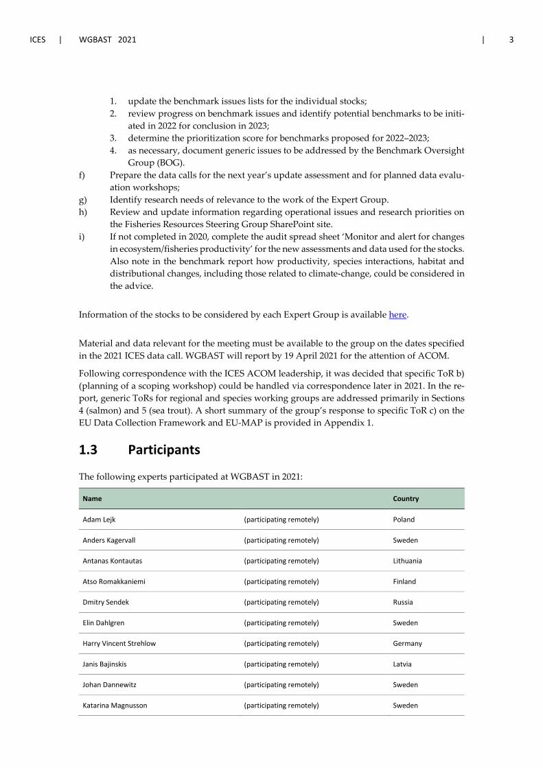
1.3 Participants
The following experts participated at WGBAST in 2021:
Name Country
Adam Lejk (participating remotely) Poland
Anders Kagervall (participating remotely) Sweden
Antanas Kontautas (participating remotely) Lithuania
Atso Romakkaniemi (participating remotely) Finland
Dmitry Sendek (participating remotely) Russia
Elin Dahlgren (participating remotely) Sweden
Harry Vincent Strehlow (participating remotely) Germany
Janis Bajinskis (participating remotely) Latvia
Johan Dannewitz (participating remotely) Sweden
Katarina Magnusson (participating remotely) Sweden
4 | ICES SCIENTIFIC REPORTS 3:26 | ICES
Name Country
Katarzyna Nadolna-Ałtyn (participating remotely) Poland
Martin Kesler (participating remotely) Estonia
Marja-Liisa Koljonen (participating remotely) Finland
Piotr Debowski (participating remotely) Poland
Rafal Bernas (participating remotely) Poland
Rebecca Whitlock (participating remotely) Sweden
Rūdolfs Tutiņš (participating remotely) Poland
Samu Mäntyniemi (participating remotely) Finland
Sergey Titov (participating remotely) Russia
Stefan Palm (participating remotely) Sweden
Stefan Stridsman (participating remotely) Sweden
Stig Pedersen (participating remotely) Denmark
Simon Weltersbach (participating remotely) Germany
Susanne Tärnlund (participating remotely) Sweden
Tapani Pakarinen (participating remotely) Finland
Tuomas Leinonen (participating remotely) Finland
Victoria Amosova (participating remotely) Russia
1.4 Code of Conduct
In 2018, ICES introduced a Code of Conduct that provides guidelines to its expert groups on identifying and handling actual, potential or perceived Conflicts of Interest. It further defines the standard for behaviours of experts contributing to ICES science. The aim is to safeguard the rep-utation of ICES as an impartial knowledge provider by ensuring the credibility, salience, legiti-macy, transparency, and accountability in ICES work. Therefore, all contributors to ICES work are required to abide by the ICES Code of Conduct.
At the beginning of the 2021 WGBAST meeting, the chair raised the ICES Code of Conduct with all attending member experts. In particular, they were asked if they would identify and disclose an actual, potential or perceived Conflict of Interest as described in the Code of Conduct. After reflection, none of the members identified a conflict of interest that challenged the scientific in-dependence, integrity, and impartiality of ICES.
ICES | WGBAST 2021 | 5
1.5 Ecosystem considerations
1.5.1 Salmon and sea trout in the Baltic ecosystem
Salmon (Salmo salar) and sea trout (Salmo trutta) are among the top fish predators in the Baltic Sea. Together with European eel (Anguilla anguilla) and migratory whitefish (Coregonus lavare-tus/Coregonus maraena) they form the group of keystone diadromous species in the Baltic Sea. Annex 2 contains background descriptions related to ecosystem aspects for Baltic salmon, in-cluding basic biology, ecological functioning, environmental pressures, disease outbreaks, ef-fects of climate change, and fisheries impacts, whereof most are common for both species. At the beginning of Section 5, a short description is also given on how the life history and ecology of sea trout differs from that of salmon.
6 | ICES SCIENTIFIC REPORTS 3:26 | ICES
2 Salmon fisheries
2.1 Overview of Baltic salmon fisheries
The fishery for Baltic salmon is heterogeneous. Commercial and recreational fisheries occur in the sea (offshore and coast) and in rivers, using a variety of gears. Below follows a brief overview of the most important fisheries and gears. A more comprehensive description of various fisheries including descriptions of gears and methods used is given in the Stock Annex (Annex 2). More extensive descriptions of this, as well as historical gear development in Baltic salmon fisheries, are also available in ICES (2003). Information on catches, effort, discards, unreporting, and mis-reporting is provided in Sections 2.2–2.4.
Commercial fisheries Coastal commercial fishing targeting salmon occurs mainly in Gulf of Bothnia and Gulf of Fin-land, along the coasts of Sweden and Finland, but to some extent also in Estonia and Latvia. Currently, this fishery stands for the majority of the commercial landings. Gears used include different types of trapnets. The fishery occurs during spring and summer and targets salmon on their spawning migration. Some commercial fisheries also exist in fresh water close to river mouths, such as in a few Swedish rivers with reared salmon and in River Daugava, Latvia.
Offshore commercial salmon fishing is mainly carried out in Southern Baltic Sea (Main Basin), although it has periodically occurred also in Southern Gulf of Bothnia. Currently the commercial offshore fishery is more or less limited to vessels from Denmark, Poland, Latvia and Lithuania, whereas earlier several other countries were also involved. Historically, driftnets were the most important gear, but after the driftnet ban was enforced in the Baltic Sea in 2008 commercial off-shore fisheries consist mainly of longlining and to some extent anchored floating gillnets. The offshore fishery takes place mainly during the period November to March, and targets non-ma-ture salmon in their feeding areas.
Recreational fisheries Recreational trolling has become a more and more popular fishing method to catch salmon in the Baltic Sea. Even though, the increase, due to various reasons, has levelled off in the latest years. So far, the trolling fishery is most developed in Sweden, Denmark, Germany and Poland. Also, in Latvia and Lithuania trolling fishery is developing. The trolling season varies between different sea areas and depends on the feeding and spawning migration of salmon and/or sea-sonal closures. In south-western Baltic Sea and Main Basin, it typically starts in late fall and ends in the middle of May. In the Åland Sea and Gulf of Bothnia, the season starts in the end of May and continues until late summer. Over the past few decades, the trolling fishery has increased, whereas the commercial offshore catches have declined. Thus, the relative importance of the rec-reational fishery has in a longer perspective increased over time.
The river fishing for salmon in the Baltic Sea region has a very long history. Until the mid-1990s, nets and weirs were used in many rivers throughout the Baltic Sea region. Currently the river fishery for wild salmon is entirely recreational and to a major part restricted to angling (rod and reel fishing). The most productive wild Baltic salmon rivers are by far the Finnish and Swedish large rivers flowing into the Bothnian Bay (SD 31). The main fishing season is between May–September, during the spawning run. Rod fishing for salmon in these rivers is very popular, attracting several thousands of anglers every year. The recreational river fishing for salmon in other countries surrounding the Baltic Sea is more limited, although salmon, to some extent, is caught in Estonian, Lithuanian, Latvian and Polish rivers. Russia has no recreational salmon
ICES | WGBAST 2021 | 7
fishery in their rivers feeding into the Baltic Sea, and no Baltic salmon rivers exist in Denmark and Germany.
While the recreational salmon fisheries is largely dominated by angling (offshore trolling and rod fishing in rivers) there are other types of recreational fisheries carried out in some countries. Where passive gears such as trapnets, gillnets or longlines are being used for catching salmon, either as a target species or bycatch, in both coastal and riverine recreational fisheries. These catches are generally estimated to be of minor importance, in terms of impact on the stocks (i.e. removals).
Brood stock fisheries Brood stock fisheries are aimed at collecting mature individuals for breeding purposes. Either within sea-ranching programmes, where mature breeders are caught annually to produce salmon for stocking, or to renew closed brood stocks kept in captivity during the whole life cycle. Brood stock fisheries usually occur in rivers with reared salmon, but adult salmon are also caught for breeding purposes in some wild salmon rivers. Catches for breeding purposes are, however, rather limited and occur in Estonia, Finland, Latvia, Lithuania, Poland, Russia and Sweden.
2.2 Catches
This section contains information on commercial and recreational Baltic salmon catches from sea, coast and rivers in 2020 and over time. The catches presented are, unless otherwise stated, landed (retained) salmon.
Commercial catch statistics provided for ICES WGBAST are based on EU logbooks, national re-porting system for vessels not obliged carrying logbook, and/or sales notes. As described in more detail in the Stock Annex (Annex 2), non-commercial recreational catches are typically estimated by a combination of different types of national surveys targeting various recreational fisheries (e.g. using access-point surveys, questionnaires, camera surveillance, etc.) and expert evalua-tions or expert opinion ‘guesstimates’. Further details on the collection of salmon catch data in the Baltic Sea (in total and by country) are given in Annex 2.
Due to the increasing share of recreational fishermen practicing catch-and-release, voluntarily or due to regulations, there is a need for separate time-series including released salmon. Further, since the effects of catch-and-release on the management of the stocks largely are unknown, re-liable data on survival rates and other effects on fish that have been caught and released are needed.
2020 data presented are principally data delivered in the ICES WGBAST and the WGBAST 2021 data calls respectively when parts of the data were still preliminary. Quality checks during the meeting resulted in a few changes in the dataset. Besides changes in conjunction with further quality checks, any future revision of data over time may e.g. be due to additional landings re-ported in the commercial fisheries or adjustments of catch estimates in the recreational fisheries.
The following seven tables with salmon catches divided in various ways (as described below) are annually updated and referred to in this report:
• Table 2.2.1.1: nominal reported and total salmon catches in weight by country for the years 2001–2020 (including discarded, unreported and misreported fish). Estimates of discards and unreported and misreported catches are presented separately.
• Table 2.2.1.2: corresponding annual catch data as in Table 2.2.1.1 in numbers. • Table 2.2.1.3: nominal reported catches in weight from sea, coast and rivers divided by
region (SD 22–29, 30–31 and 32) and country for the years 2001–2020. • Table 2.2.1.4: corresponding annual catch data as in Table 2.2.1.3 in numbers.
8 | ICES SCIENTIFIC REPORTS 3:26 | ICES
• Table 2.2.1.5: nominal catches from last year (2020) in weight and numbers from sea, coast and river, divided by country and by SD.
• Table 2.2.1.6: nominal commercial landings in numbers (2001–2020) from sea and coast com-pared to TAC, divided by fishing nation and region (SD 22–31 and 32).
• Table 2.2.1.7: nominal recreational (non-commercial) catches in numbers from sea and coast (pooled) and rivers, divided by country and region (SD 22–31 and 32) in 2001–2020.
In addition to tables, a number of figures on salmon catch data are also presented that illustrate catch development over time.
The estimated discards, unreported and misreported catches are not included in the nominal reported catches, but presented separately. The estimated catches are calculated using conver-sion factors and reported in terms of the most likely value with a 90% probability interval (PI). More details on the estimating procedures are given in Section 2.3 (see also the Stock Annex, Annex 2, Section B.1.3). In the Stock Annex, an overview of management areas (regions) and rivers is also presented.
2.2.1 Catch development over time
There has been a long-term decline of the total nominal catches in the Baltic Sea, starting from 5636 tonnes in 1990 down to just 926 tonnes in 2010. After that, the catches have remained rather stable up to 2017 when the historically lowest total nominal catch was registered: 797 tonnes. In 2018 catches increased again and in 2020, the total nominal catch was 912 tonnes (Table 2.2.1.1) or 145 294 salmon (Table 2.2.1.2). Where the weight and the numbers were slightly lower than in the previous year.
After the driftnet ban was enforced in 2008, the percentage of the total commercial offshore catch by this gear has been zero. At the same time, commercial catches with trapnets along the coast increased their share. Consequently, the proportion of the coastal catch has gradually increased over time, and in 2020, it was 46% out of the nominal total catch (in weight) (Table 2.2.1.3). In the same year, approximately 69.3% of all commercial catches (in weight) were taken in coastal trap (or fyke) nets.
Over the years, the total share represented by river catches has been fluctuating. However, in the latest years they have remained rather stable, being approximately 30% of the total (in weight). In Table 2.2.1.3 the distribution of total catches (in weight) from offshore, coastal and riverine fisheries are presented (see Table 2.2.1.4 for corresponding catches in numbers). The distribution of nominal catches in 2020 by country, per subdivision, offshore, coast and river are presented in Table 2.2.1.5.
A comparison of landings (coastal and offshore) per country compared to the EU TAC in 2019 is presented in Section 2.2.3. Compiled information on landings versus TAC is also presented in Table 2.2.1.6. Note that data presented in Section 2.2.3 are the latest available. Discards, unre-ported and misreported catches are not included in the utilisation of the TAC, but in Figure 2.2.1.1 total catches of salmon are presented (as a percentage of TAC) where such catches have been added. In this figure, the recreational landed catches are also included.
A notable change in the catch distribution occurring in the past few decades is that the propor-tion of non-commercial catches has grown in relation to the commercial catches. The develop-ment for the proportion of non-commercial catches (including river catches and expert trolling estimates) from 2001 and onwards is illustrated in Figure 2.2.1.2. In 1994, non-commercial catches comprised just 10% of the total nominal catches (in weight), whereas since 2013 the share has fluctuated between 40 and 50%. Nominal recreational (non-commercial) catches in numbers
ICES | WGBAST 2021 | 9
from sea and coast (pooled) and rivers in 2001–2020, divided by country and regions (SD 22–31 and 32), are presented in Table 2.2.1.7.
In 2020, WGBAST continued the work initiated in 2017 to pay extra attention to the recreational salmon fisheries that are becoming proportionally more important. For the growing trolling fish-ery, a time-series of trolling catches from an expert elicitation initiated in 2017 (ICES, 2017a; 2017c) was updated (Figure 2.2.1.3). The estimates were partly updated until 2020, to take into account new information from earlier years received from new surveys. The update resulted in a slightly modified time-series compared to in previous years, with lower annual estimates for some years. The estimates are, however, still more than 20 000 salmon larger than previously assumed (i.e. for the 2010–2016 assessments). Trolling catches from the Main Basin (SD 22–28) are dominating, and are only to a lesser degree taken in SD 29–32. Catches in the Main Basin have been declining since 2015, but in 2019, an increase was observed, however in 2020 catches declined again. The 2020 Main Basin estimate was about 19 720 salmon caught and retained, including estimated post-release mortality (Figure 2.2.1.3). In contrast to 2017, when the assess-ment model for salmon in AU 1–4 did not perform, the new updated trolling catch estimates have been included in later years’ stock assessments (Section 4).
In subdivisions 22–31, the total recreational river catch in 2020 was noticeably bigger than in previous years with 37 396 salmon retained. In SD 32, the river catch in 2020 was 438 salmon. Compared to 2019, this was a slight increase, however there is a strong downward trend in the SD 32 recreational river catches since the beginning of the 2000s (Figure 2.2.1.4). No further anal-ysis of the recreational river catches has been made. In Section 3.1, details on specific river catches are presented.
2.2.2 Catches by country (2020)
Denmark: The Danish salmon fishery is an open sea fishery. The total commercial and recrea-tional catches (excluding discards and seal damaged salmon estimates) in 2020 were 11 065 salmon. The amount of discarded BMS salmon was negligible while the number of seal damaged salmon according to logbooks was 1452. All catches, including the recreational, were in ICES SD 24–25. The commercial fishery uses longlines and it takes place from late autumn to spring (Oc-tober–May). The effort in the commercial salmon fishery has decreased in recent years. Com-pared to 2019 the effort was reduced by 46%. The most likely reason for this is heavy seal preda-tion. The commercial landings in numbers in 2020 was 3000, which is significantly lower than the 2019 landings (6009). The commercial landings in weight in 2020 was 16.6 tonnes (2019: 29.8 tonnes). The recreational fishery is mainly trolling, but some recreational passive gear fishing, i.e. longlining, also takes place in waters close to Bornholm. It is likely that the effort in this fish-ery has decreased in recent years with the increasing number of seals around Bornholm. It is guesstimated that catches are very small (<100 salmon per year). An estimate resulting from an Internet based recall survey in 2020 targeting annual licence holders yielded a result of 8065 salmon landed for trolling alone. However, the result is believed to be an overestimate due to recall- and avidity bias as respondents participating in such surveys often are the most avid an-glers and the recall period is long (6 month). An on-site survey has been established to adjust the recreational catch estimates from the off-site survey. From the off-site survey the estimated num-ber of salmon caught and released in 2020 was 3835 salmon.
Estonia: There is no specific Estonian salmon fishery. In the coastal fishery, salmon is a bycatch and the main targeted species are sprat, flounder and perch. The share of salmon in the total coastal catch is less than 1%. In 2020, similar to in previous years the Estonian salmon sea catch was below 1 tonne. The coastal catch (commercial and recreational) was 13.3 tonnes, which is slightly higher than 2019 catches (11.6 tonnes). The vast majority of salmon is caught in the Gulf of Finland (SD 32). There are about 570 commercial fishermen in Gulf of Finland, and in addition
10 | ICES SCIENTIFIC REPORTS 3:26 | ICES
up to 6433 monthly gillnet licences are distributed annually (standard length of a net is 70 me-ters). The commercial fishery takes 68% of the total catch. The vast majority of the salmon (88%) is caught in gillnets and the rest in trapnets. About 75% of the annual catch is taken in September, October and November. Nearly all caught salmon are spawners.
Finland: In 2020, Finnish fishers caught a total of 54 211 salmon (384 tonnes) in the Baltic Sea, which was 4% less than in 2019. The landed commercial catch was 28 606 salmon (187 tonnes). The recreational catch (including river catches) was 25 605 salmon (178 tonnes). Practically all commercial catch was taken in the coastal fishery mainly by trapnets and there was no salmon fishing in the southern Baltic Sea by the Finnish vessels. Commercial catch data for the year 2020 are preliminary. Recreational catch estimates in the sea for the years 2018–2020 are based on the results of the Finnish Recreational Fishing 2018 survey. National surveys are carried out every second year and for years with missing data the same sea catch estimates as the latest survey is assumed. Catch estimate of the recreational fishery in the sea was assumed to be the same as for the year 2018 (the latest survey year) and highly uncertain (39 t, CV>50%). River catch was 20 105 (138 tonnes) increasing 20% from 2019.
Finnish professional fishermen mainly use trapnets. In 2020, 158 coastal fishermen caught salmon with 343 trapnets, and total effort in the trapnet fishery was 18 453 gear days, about 6% more than in previous year. Reported discards of seal damages were 2200 salmon (13 tonnes) about the same as in previous year comprising about 7% of the total commercial catch.
Commercial salmon catch in subdivisions 22–31 was 20 589 salmon (132 tonnes) (commercial catch data from the River Iijoki and River Kemijoki is not available yet)). Recreational catch was 25 220 salmon (176 tonnes) of which 19 920 was caught from rivers (most from the River Torni-onjoki). According to the national survey in 2018 about two thirds of recreational sea catch was taken from the Gulf of Bothnia (5300 salmon, 39 tonnes, notice high uncertainty CV>50%). In the coastal fishery 127 fishermen caught salmon with 257 trapnets. The total fishing effort was 11 099 trapnet days about the same as year 2019 (data are preliminary). In Åland Islands, about 1250 salmon (10.5 tonnes) were caught with anchored floating nets. Discards of seal damaged salmon were 1450 fish (9 tonnes) comprising 7% of total commercial catch in subdivisions 29–31. The total fishing quota was 24 178 salmon (=22 370 salmon + 1808 salmon of transferred unutilized quota from previous year) in management unit 22–31. The quota was utilised to 85%.
Commercial salmon catch in Subdivision 32 was 8017 salmon (54 tonnes) and it was taken in the coastal fishery. Recreational catch in the area was 385 salmon (2 tonnes). River catch (all recrea-tional) was 185 salmon (1 tonne) and almost all of it was taken from the River Kymijoki. In 2018 (the latest survey year) the recreational catch the Gulf of Finland was very small (200 salmon, 1 tonne, CV>50%) compared to previous estimate in 2016. The 2016 estimate is probably a rich overestimate, and 2018 estimate an underestimate. Practically all commercial salmon catch in the area was taken by trapnets. In all 31 fishermen fished salmon with 86 trapnets with the effort of 7354 trapnetdays being 12% more than in 2019. Discards of the seal damaged salmon were 750 fish (4.5 tonnes) being 9% of the total commercial catch in the area. The fishing quota was utilised to 83% of total 9679 salmon (= 8708 salmon + 971 salmon of transferred unutilized quota from the previous year).
Recreational catch at sea is estimated with a national off-site survey. The last survey covers the year 2018 and was conducted in 2019. The 2020 survey is ongoing and results will be published in October 2021. Salmon and sea trout catch estimates are highly uncertain because these fishers are rare in the total population. Note that in this national survey, salmon (and sea trout) catch estimates are highly uncertain because these fishers are so rare in the total population (just 17 salmon trollers among all respondents). National surveys are carried out every second year. For the missing ‘odd’ years, the same sea catch estimate as in the preceding year is assumed. The catch estimate in 2016 was 55–137 tonnes (7000–17 000 salmon). Results suggest that almost 90%
ICES | WGBAST 2021 | 11
of the catch was taken by trolling. In 2017, the Finnish Federation for Recreational Fishing con-ducted a questionnaire among salmon trolling skippers (92 replies were received). The skippers are considered to represent the most active part of all trolling fishers. An expert estimate of the total number of active trolling boats in Finland is 300–400. In addition, about the same amount of less active boats exist that only go to sea 1–2 days per year (maybe not even for trolling). The responding skippers fished on average eight days in 2017 (range: 0–25 days) and the average catch was 0.2 salmon per fishing day in the Gulf of Finland and 0.4 salmon per fishing day at the Åland Islands and in Gulf of Bothnia. Extrapolation of these parameters to the estimated whole fleet suggests a total catch of about 300–1600 salmon in 2017.
Germany: The total reported commercial salmon catch in 2020 (SD 22–24) in numbers was 512 with a total weight of 25. tonnes (using a mean weight of 5 kg per salmon). In recent years, vir-tually no German commercial fishery has directly targeted salmon; hence, most of the salmon are caught as bycatch in other fisheries (mainly passive gear fisheries). The German TAC for 2019 was 1996 salmon (total for subdivisions 22–31) and the quota was utilized to 25.4%.
Recreational salmon fishing occurs almost exclusively from trolling boats in the waters off the island of Ruegen (SD 24) in Germany. Since 2017 (pilot in 2016), a regular survey has been estab-lished to monitor the recreational salmon trolling fishery in Germany. Recreational salmon boat fishing effort is evaluated by trolling boat trip counting via remote cameras in three relevant marinas on the island of Ruegen (covering ~60 % of the total fishing effort) during the salmon trolling season from December until May (see Kaiser (2016), ICES (2018) and Hartill et al. (2020) for details). Salmon trolling effort from marinas not monitored by cameras (n = 4) is extrapolated using monthly (in 2019 every two weeks) instantaneous trolling boat counts covering all marinas and the proportions of boats that went out for fishing derived from the marinas with camera monitoring. The camera monitoring is complemented by random on-site interviews of trolling anglers in four relevant marinas (including the marinas where the trolling boat trip counting was conducted) to determine catch per unit of effort in order to estimate catches and collect biological catch data and socio-economic information. In 2020, a total of 60 random on-site samplings were conducted and 252 trolling boats with 513 anglers targeting salmon were interviewed. The total number of retained salmon was estimated to be 1093 (95% CI: 556–1654) salmon in 2020. In ad-dition, 258 salmon have been released, resulting in a release rate of 2.3%.
There are no data available on freshwater salmon catches. However, commercial and recreational salmon freshwater catches are most likely insignificant as there are no rivers with significant salmon spawning migration and fishery along the German Baltic coast.
Latvia: The Latvian salmon landing statistics are based on the logbooks and landing declarations from the offshore and logbooks from coastal and inland fisheries. Landing data from a small-scale recreational fishing in the river Salaca and Venta are based on questionnaires. In 2020, the total number of Latvian salmon landings (commercial, recreational and brood stock fisheries) was 3585 salmon (15.2 tonnes).
Salmon commercial landings in the open sea (offshore) was 7.4 tonnes which is smaller amount than in 2019. Coastal landings (commercial and recreational) were 3.9 tonnes, which is similar to the last year. Vast majority of salmon was caught in SD 28. Commercial fishermen comprised only 48,5% of the total costal landings in 2020, the rest was taken by recreational fisherman (fish-erman without rights to sell the caught fish). In 2020, vast majority of salmon in the sea was caught by longlines and gillnets. In 2020, biggest salmon landings in coastal fisheries registered during March and September, but in the offshore fisheries during March and December.
Small-scale commercial fishery exists in Daugava river up to Rigas HPP and in Daugava river connection with Lielupe river mouth called Buļļupe river (both with reared salmon). Due to large number of grey seal in the Daugava river mouth, catches in this fishery are decreasing.
12 | ICES SCIENTIFIC REPORTS 3:26 | ICES
In the rivers where natural reproduction of salmon occur, all angling and fishing for salmon and sea trout is prohibited with exception of licensed angling for sea trout and salmon kelts during the spring season in the rivers Salaca, Venta and starting from 2020, also Gauja river.
In total 443 retained salmon and 772 retained sea trout kelts were reported in licensed angling in 2020. Biggest share of salmon and sea trout was caught in the Salaca river. From reported 476 salmon and 602 sea trout kelts, 86 salmon and 108 sea trout have been released back alive, the rest were kept. In Gauja river, 53 salmon and 381 sea trout kelts reported in licensed angling from which 103 sea trout have been released back alive.
Lithuania: Lithuanian salmon catch statistics are based on logbooks. In 2020, Lithuanian fisher-men caught 2813 salmon (16.4 tonnes). This is a large increase compared to the last year. Largest part was caught in sea: 1.14 tonnes, and the rest (0.15 tonnes) in the Curonian lagoon. Recrea-tional catch in coastal area was 9.6 t (1621 individuals, including trolling) which is higher than in previous years.
Commercial salmon fishery is banned in all Lithuanian rivers. Recreational fishery for salmon is allowed (together with sea trout) only in designated rivers on license basis. In 2020, the number of licences sold for salmon and sea trout is still not reported by the Ministry, the number of licences sold in year 2019 was 24 435.
Poland: Total sea, coastal and river commercial catch was 6705 salmon (37.40 tonnes). Total catch was basically unchanged compared with 2019. Main gears in use for salmon are the same as for sea trout and this is why the vessels have fishing licences for both species. Main gear in salmon fishery was LLD, 77% of offshore catch, and GNS, 85% of coastal catch. Other gears were: fykenets and trawls. Commercial sea and coastal catch statistics are based on e-logbooks of ves-sels longer than 12 m and on monthly reports of vessels smaller than 12 m. Most of the catch (76%) was taken from Subdivision 26. Out of the total catch, the coastal catch was lower (28%), then offshore (71%). Salmon fishery in Subdivision 24 was occasional. All fish was caught within Polish EEZ.
Until the year 2019, the most important factor to distinguish the coastal vs offshore catches in Polish EEZ was the length of the fishing vessels: coastal if vessels were smaller than 10 m, off-shore if vessels were 10 m long or longer. Such a rule does not reflect the reality, because small boats nowadays are able to operate in offshore waters (more than 4 miles from the coast line) and vessels longer than 10 m might operate in coastal waters (up to 4 miles from the coast line). Therefore, it was decided to use the fishing location (statistical fishing squares) as the main factor to distinguish coastal vs offshore catches for 2019 and 2020 data.
Pilot study relating to salmon and sea trout recreational fisheries was conducted in 2017–2019. More details of this work were described in Polish National Report for 2017. Based on the results of the Pilot Study, sampling programme was included into regular sampling since 2020. In 2020, trolling boats have been observed in ten harbors, i.e. Władysławowo, Kuźnica, Jastarnia, Hel, Gdańsk Górki Zachodnie, Gdynia, Łeba, Ustka, Darłowo, Kołobrzeg, Mrzeżyno and Dziwnów with particular importance of Hel, Gdynia, Gdańsk Górki Zachodnie, Kołobrzeg harbours. A total of 125 different active trolling boats had been inventoried in 2020. Number of active trolling boats varied between autumn/winter (87–94) and spring (103–107) seasons with a higher number of trolling boats in spring. On this time, there is no reliable information about CPUE (expressed as a number of fish per boat per day) depends on season and total number of trolling operations (boat-days) per year. The mean CPUE for 2020 was 1.9 salmon per trolling trip/day. The prelim-inary trolling catch estimates for 2020 are 4750 landed (retained) salmons and 190 released salm-ons (below minimum landing size fish). Because of COVID-19 issue, the catches have been af-fected by lower activity of trolling anglers, and national restrictions (lock-down). It is planned to update catch data for 2018–2020, based on obtained results. The estimated sea trout bycatch
ICES | WGBAST 2021 | 13
during salmon trolling trips in 2020 is 132 individuals (retained). The coastal sea trout catch es-timates including coastal trolling targeting sea trout for 2020 was 81 713 fish.
A pilot study of estimation of Polish river recreational catches has begun in 2017 and was con-tinued in next three years. First on three rives: Ina (SD 24), Rega and Słupia (SD 25) and from 2018, also on Parsęta River (SD 25). In 2020 three new rivers were added to the survey: Łeba, Reda (SD 25) and Drwęca River (SD 26). The method used is based on catch records provided by fishing users supplemented with data from on-site surveys of anglers carried out according to the same schedule on the rivers studied. The data obtained from the catch records are delayed by two years, which results from the fishing fee system. No river data are submitted to WGBAST yet.
Russia: In 2020, 752 salmon (3.4 tonnes) were caught in Russian fisheries. There is no specific Russian salmon fishery but a small number of salmon (30 fish) was reported as bycatch in the coastal fishery. The largest part of the reported catch is from brood stock fishing in River Neva (322), River Narva (306) and River Luga (31). In addition, 63 salmon were caught in scientific fishing. The catches in recreational fishing is currently unknown.
Sweden: The total salmon catch in 2020 was 56 841 salmon (336 tonnes). In 2020, the total number of salmon in the commercial sea fishery was 23 297 (147 tonnes). Coastal fishery with trap- and fykenets made up more than 99% of the commercial coast and sea salmon catches. In addition, commercial fishing in Additionally, commercial trap net fisheries in freshwater is increasing in SD 31 in river Luleälven were a total of 15 089 salmon were landed. Total weight of the commer-cial riverine salmon catches were 61.3 tonnes. Besides River Luleälven commercial fishing in freshwater exists in reared rivers in SD 30, but this year’s data were still not available and will be updated in the next data call.
Recreational fishing in Sweden have two main components, angling in rivers and trolling at open sea. River catches are estimated using catch reports from anglers combined with expert evalua-tions of unreported catch (using local experts). The quality of the data varies a lot and in rivers with developed fishing tourism and active management nearly all of the catch is reported. In other rivers most of the catch numbers are based on the expert evaluation. The 2020 catch of recreational fishers in rivers was 16 039 salmon (112 tonnes).
For the trolling fishing method development continued in 2020 with an on-site interview study in the two most popular harbours Simrishamn and Ystad were surveyed between 2020-03-23 and 2020-05-10. A total of 27 days, when all returning trolling boats were interviewed, was randomly selected and data on catches were obtained. The number of landed salmon during the survey period landed in Simrishamn and Ystad was estimated to 377 (CI 163–592) and 426 (CI 93–760) salmon released. The estimates from Simrishamn and Ystad were the raised to the catch in SD 25–29 during the full year with the assumption that the catch was distributed, in time and space, was distributed in similar way as in earlier studies. This resulted in an estimated total catch of 2416 (15.7 tonnes) salmon landed and 2730 salmon released in SD 25–29.
2.2.3 Landings by country compared with the EU TAC 2020
The total allowable catch (TAC) or fishing opportunity for Baltic salmon in 2020 was stated in COUNCIL REGULATION (EU) 2019/1838 of 30 October 2019. In SD 22-31, 66% of the original TAC of 86 575 individuals was utilized and in SD 32, 97% of the original TAC of 9703 individuals was utilized.
14 | ICES SCIENTIFIC REPORTS 3:26 | ICES
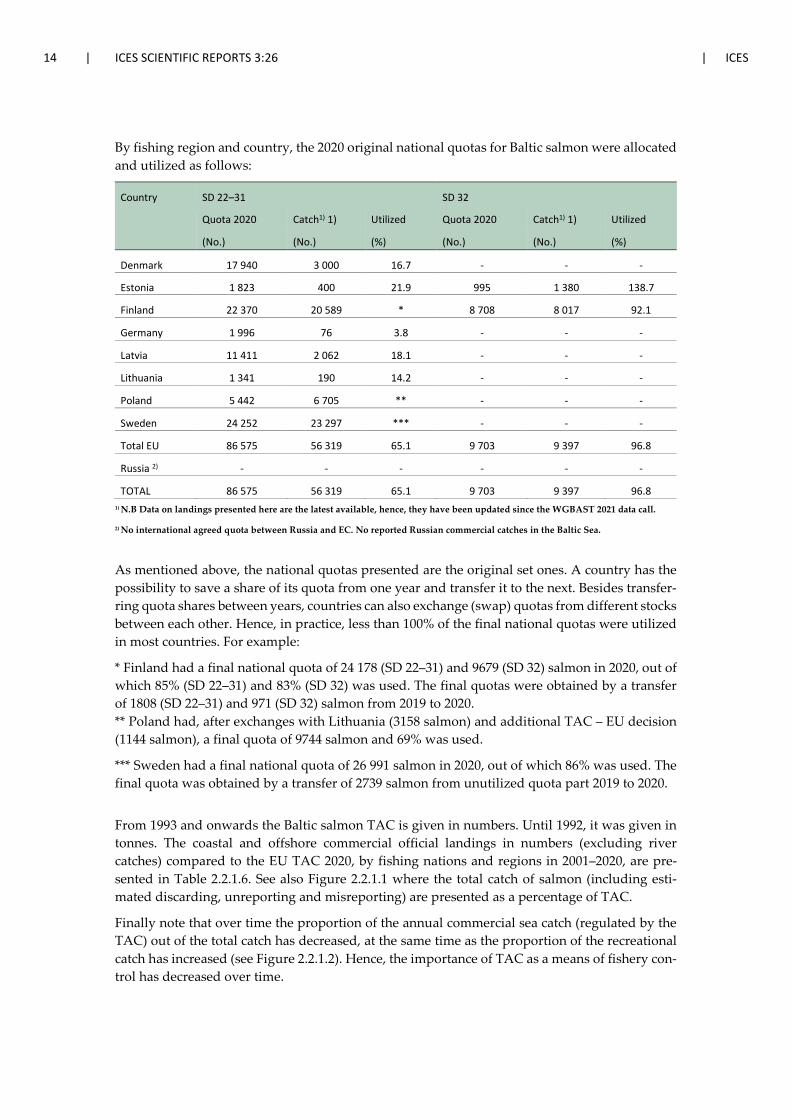
By fishing region and country, the 2020 original national quotas for Baltic salmon were allocated and utilized as follows:
Country SD 22–31 SD 32
Quota 2020 Catch1) 1) Utilized Quota 2020 Catch1) 1) Utilized
(No.) (No.) (%) (No.) (No.) (%)
Denmark 17 940 3 000 16.7 - - -
Estonia 1 823 400 21.9 995 1 380 138.7
Finland 22 370 20 589 * 8 708 8 017 92.1
Germany 1 996 76 3.8 - - -
Latvia 11 411 2 062 18.1 - - -
Lithuania 1 341 190 14.2 - - -
Poland 5 442 6 705 ** - - -
Sweden 24 252 23 297 *** - - -
Total EU 86 575 56 319 65.1 9 703 9 397 96.8
Russia 2) - - - - - -
TOTAL 86 575 56 319 65.1 9 703 9 397 96.8 1) N.B Data on landings presented here are the latest available, hence, they have been updated since the WGBAST 2021 data call.
2) No international agreed quota between Russia and EC. No reported Russian commercial catches in the Baltic Sea.
As mentioned above, the national quotas presented are the original set ones. A country has the possibility to save a share of its quota from one year and transfer it to the next. Besides transfer-ring quota shares between years, countries can also exchange (swap) quotas from different stocks between each other. Hence, in practice, less than 100% of the final national quotas were utilized in most countries. For example:
* Finland had a final national quota of 24 178 (SD 22–31) and 9679 (SD 32) salmon in 2020, out of which 85% (SD 22–31) and 83% (SD 32) was used. The final quotas were obtained by a transfer of 1808 (SD 22–31) and 971 (SD 32) salmon from 2019 to 2020. ** Poland had, after exchanges with Lithuania (3158 salmon) and additional TAC – EU decision (1144 salmon), a final quota of 9744 salmon and 69% was used.
*** Sweden had a final national quota of 26 991 salmon in 2020, out of which 86% was used. The final quota was obtained by a transfer of 2739 salmon from unutilized quota part 2019 to 2020.
From 1993 and onwards the Baltic salmon TAC is given in numbers. Until 1992, it was given in tonnes. The coastal and offshore commercial official landings in numbers (excluding river catches) compared to the EU TAC 2020, by fishing nations and regions in 2001–2020, are pre-sented in Table 2.2.1.6. See also Figure 2.2.1.1 where the total catch of salmon (including esti-mated discarding, unreporting and misreporting) are presented as a percentage of TAC.
Finally note that over time the proportion of the annual commercial sea catch (regulated by the TAC) out of the total catch has decreased, at the same time as the proportion of the recreational catch has increased (see Figure 2.2.1.2). Hence, the importance of TAC as a means of fishery con-trol has decreased over time.
ICES | WGBAST 2021 | 15
2.3 Discards, unreporting and misreporting of catches
Data on discards in the commercial fisheries are to some extent reported in the official statistics, and the latest country specific information on this is presented in Section 2.3.2. However, the quality of these data is very unsure. Therefore, additional estimates are made (see below). For obvious reasons, there are no official reports of unreported and misreported catches. However, for some countries, information collected from diverse sources is still available. In Section 2.3.3, the issue of misreporting is elaborated on further.
Data for the period 1981–2000 on discards and unreporting of salmon from different commercial fisheries in the Baltic Sea are incomplete and fragmentary. For years 2001–2020 the estimates for discards and unreporting have been computed with a new method based on updated expert evaluations (adopted in WGBAST 2013). The resulting parameter values for the elicited priors and pooled (average) probability distributions for different conversion factors are given in Table 2.3.1. In WGBAST 2021, mostly the same parameter values were used for 2020 fisheries as for previous years fisheries, because experts saw the situation remained unchanged in terms of dis-carding, unreporting rates, proportions of BMS salmon and seal damages. Only the rate of unre-porting in the Polish coastal fisheries was updated with a slightly lower estimated in 2020 and 2019 from earlier years. For detailed information about estimation procedures for these conver-sion factors, see Stock Annex (Annex 2, Section B.1.3).
A main part of discards is seal damaged salmon, which occurs in the coastal trapnet and gillnet fishery, but also in the offshore longline fishery (Table 2.3.2.). In the offshore fishery, it is small amounts of undersized salmon that are estimated to be discarded. Since 2015, there has been a landing obligation for the longline fishery; however, it has not been fully implemented since little reporting of such landings has occurred. Estimates for discards, unreporting and misreporting by management area are presented in Table 2.3.3. The estimates are uncertain and should be considered mainly as an order of magnitude.
In the recreational fisheries on the other hand, almost no data on discarded (caught and re-leased), unreported and misreported catch are collected, and no estimates are currently made by WGBAST.
2.3.1 Estimated discards
In 2020, approximately 5300 salmon are estimated to have been discarded due to seal damages in the Baltic Sea. About half of discards took place in the fishery in the south Baltic Sea (longline and other gears) and other half in the coastal trapnet fisheries in the northern Baltic Sea (Table 2.3.2). Estimates were based on the observed proportion of seal damaged catch in subsamples that has been extrapolated to the total catch. In this calculation, also potential misreporting and unreporting were accounted in the total catch. In WGBAST 2019, the Danish expert evaluation was updated retrospectively for years 2016 and 2017 using the same estimate as for 2018. Basis for the update was that there were no logbook data on discarded seal damaged salmon from Denmark in 2016–2017 and the previously estimated discard rate of 50% (5–65%) was based on sparse observer data in 2016 (i.e. no data in 2017). In 2018–2020, logbook records on seal damages were available from the Danish and Polish longline fisheries. The amount of seal damaged catches in the Main Basin have increased gradually to significant rates starting around 2013, as a result of increase in grey seal population in the area. In 2020, the proportion of seal damaged salmon in the total catch was 33% in the Danish and 38% in the Polish fisheries.
In the northern Baltic Sea, seal damages started to escalate gradually from 1993, but since the introduction of ‘seal safe’ trapnets, the catch losses in coastal fisheries have levelled off. In 2020, the total seal damaged discards were about 1900 salmon in the Gulf of Bothnia and 750 salmon
16 | ICES SCIENTIFIC REPORTS 3:26 | ICES
in the Gulf of Finland. Most of the damages were reported from Finnish coastal trapnet fisheries. In Finland, data on seal damages are based on logbook records. In Sweden, the level of seal dam-ages is estimated based on data from a voluntary logbook system and available data on seal interaction in the official statistics, for which an additional expert assessment has been made. The reported amounts of seal damaged salmon should, however, be regarded as a minimum estimate.
The reporting rate of the seal damaged catch is assumed to be the same as for the undamaged catch in the coastal fishery. For the time being, logbook-based data on numbers of sea damaged salmon is available from Finland, Sweden and in 2018–2020 also from Denmark and Poland. However, the reported amounts of sea damage salmon are minimum estimates and true volumes are potentially higher. In other countries, estimates are based on proportional damage rates de-rived from either logbook or expert evaluation.
Dead discards of undersized salmon in 2020 were estimated to about 700 salmon in the whole Baltic Sea (Table 2.3.2). Proportions of undersized salmon in the catches of different fisheries are mainly based on sampling data (Table 2.3.1) and are considered rather accurate. Mortality esti-mates of the discarded undersized salmon released back to the sea are based on expert opinions. Mortality of the undersized salmon released from longline hooks back to sea is currently as-sumed to be high (around 80%), but few studies have been carried out on this issue and the true rate is uncertain. In the trapnet fishery, post-release mortality is assumed to be lower (around 20%), but again the true rate is uncertain. Both the experimental design and the settings to study these mortalities are challenging, but such empirical studies are needed in order to get better estimates on the survival rate of salmon discarded.
Post-smolts and adult salmon are frequently caught as bycatch in pelagic commercial trawling for sprat (mostly for supplying fish for production of fishmeal and oil), but are probably often unreported in logbooks because the relative amount of salmon in these catches is low and can be identified only during unloading (ICES, 2011). Because of insufficient data, however, estimates of these potential removals are so uncertain that they are not considered in the present assess-ment. Only the reported catch from the trawls is accounted for in the catch data, although it has been very low over the years.
2.3.2 Reported information by country
Below follows country specific information on reported discards (seal damaged fish or fish al-lowed to discard), and for some countries, short general information on seal interactions is also included. If available, any records on eventual unreporting and misreporting of catches are pro-vided.
Denmark has not information from which it is possible to estimate trustworthy discard percent-ages. Since the quota for salmon in recent years has not been fully utilized, it seems unlikely, however uncertain, that there are unreported catches in the professional salmon fishery. The potential unreported landings would likely be the largest salmon with a weight > 7.9 kg, as these salmon cannot be landed for human consumption.
The bycatch of salmon in other fisheries has been observed to be quite low. Observers from DTU-Aqua participated in the herring and sprat fishery in the Baltic in the winter 2007/2008 for about 50 days, and bycatches of salmon were insignificant in this fishery.
In Estonia, the seal damages are serious problem in salmon and sea trout gillnet fishery. Accord-ing to the personal communications of fishermen damages are very common. Quantitative as-sessment of damages is not available as fishermen in most cases did not present claims for gear compensation.
ICES | WGBAST 2021 | 17
In Finland reported discards of seal damages were about 2200 salmon (13 t) about the same as in previous year. Seals caused severe damages to all fisheries mainly in subdivisions 29–32 where seal damages comprised about 7% of the total commercial catch in the region. Other discards (seagulls, cormorants, etc.) were 20 salmon. The compensation of seal damages is based on rec-orded catches (all species accounted), which is considered to improve the catch reporting. The rate of unreporting of catches is considered to have decrease to a very low magnitude as a con-sequence of the recent developments in the fishing regulations. In 2017, an individual quota sys-tem was initiated and since then also all landed salmon have had to carry a landing mark which probably steers to a careful catch reporting. There are no available records of misreporting.
In Germany there are no data available on predation by seals. The current seal population in German Baltic waters is small but increasing. No seal damaged salmon have been reported to the authorities in 2020. Concerning the current seal density and the low level of the commercial catches, it seems unlikely that predation by seals is an important issue in the commercial fishery in German waters. However, this situation may change in the future. Furthermore, German com-mercial fishers reported increased predation rates on salmon longline catches around the island of Bornholm in recent years, which has led to the cessation of the directed salmon fishery by German vessels in 2016.
In Latvia information on seal predation in trapnet and gillnet fisheries of salmon and trout is available from coastal fishery logbook statistics. Reported direct catch losses from logbook sta-tistics was 8% of the total salmon catch and 16.5% of the total sea trout catch. The inspection of logbooks reveals also high seasonal and spatial variation of catch damage. This was not consid-ered in estimation of Latvian fishery total catch damage. Thus, the data should be treated with caution. Damaged catch (direct catch loss) for salmon and sea trout in 2020 by numbers were estimated applying average weight of fishes in landings to reported catch damage in logbooks. There is no data on other types of salmon discards.
In Lithuania, reported data of seal damages, discards, unreporting and misreporting are not available.
In Poland, seal predation of 352 salmons and 235 sea trout were recorded in logbooks in 2020 and reported to Fishery Monitoring Centre (FMC). This is less than 2019 (422 SAL; 258 TRS). In addition, 2802 salmonid fish (both salmon and sea trout) have been reported to the Ministry of Maritime Economy and Inland Waterways in 2020. This is higher than in 2019 when 1978 fish, both salmon and sea trout were reported. Number of reported fish concerns to 268 individual reports. No information on site. Based on Regulation (EU) No 508/2014 of the European Parlia-ment and the European Council, on the European Maritime and Fisheries Fund, this Regulation gives the possibility to EU Member States to finance compensation from EMFF funds for losses caused by birds and mammals in sea areas. The seal damages occurred in 3.7% of fishing trips targeting salmon or sea trout. The mean value (%) of seal damaged salmonid fish in catch where the losses have been reported was 53.7% (median = 50.0%; min = 0.9%; max = 100%). Most of the reports came from the Gulf of Gdańsk. Misreporting of salmon as sea trout in the Polish fisheries is treated below (Section 2.3.3).
In Russia, no information on seal damages, discard, unreporting and misreporting is available. However, unofficial information indicates presence of significant poaching of salmon and sea trout, both in the coastal area and in rivers.
In Sweden, a total of 437 salmon were reported as seal damaged in 2020, all in the commercial coastal fisheries. In 2019, the total number of reported seal damaged salmon in the Swedish fisheries was 480. Since the possibility to record number of seal damaged fish was initiated, the reported number has been fluctuating and the latest years an increasing trend is seen. If this is due to an actual increase in the damage rate or if the willingness of the fishermen to report seal damaged fish has increased is unclear. If this is due to an actual increase in the damage rate or if
18 | ICES SCIENTIFIC REPORTS 3:26 | ICES
the willingness of the fishermen to report seal damaged fish has increased is unclear. Logbook data on discards and seal damage are likely incomplete (see below), therefore earlier estimates of the proportions discard, misreporting and unreporting of total catch are still the best available, see WGBAST 2020 report Table 2.3.1.
In the logbooks, it is possible, but not mandatory, to record seal damaged fish. If you report seal damaged fish they are saved as a special catch category in the official statistics. Seal damaged fish are not counted into the quota and in fisheries where the landing obligation is put in practice, seal damaged salmon do not have to be landed.
Data on seal damages in the Swedish official catch statistics from the commercial coastal (and off-shore) fisheries do not include a quantitative measure of injured fish. Instead, the information requested is whether you have caught any seal damaged fish or if your gear has been seal dam-aged during a fishing trip. A trip with seal damages is then tagged with a specific “reason code”. No information on seal damages is collected from the commercial river fisheries.
2.3.3 Misreporting of salmon as sea trout
From 2019, it has been prohibited to fish for sea trout beyond four nautical miles and to limit bycatches of sea trout to 3% of the combined catch of sea trout and salmon in order to contribute to preventing misreporting of salmon catches as sea trout catches (Council Regulation (EU) 2018/1628 of 30 October 2018 fixing for 2019 the fishing opportunities for certain fish stocks and groups of fish stocks applicable in the Baltic Sea and amending Regulation (EU) 2018/120 as re-gards certain fishing opportunities in other waters). This regulation in combination with unfa-vourable weather conditions and increasing seal damages, had a major impact on the Polish fish-eries in 2019 and 2020. Both the effort and the total catch in the offshore fishery were reduced and misreporting of salmon as a sea trout disappeared almost completely (estimated misreport-ing was only 600 and 200 salmon in 2019 and 2020 respectively). The coastal fisheries targeting sea trout, increased in 2019–2020 compared with previous years. Although there is no wild or mixed salmon rivers in Poland, about 1100 salmon were reported in the coastal waters in 2020. Although the sampling intensity is not fully representative for the whole fishery, the limited biological sampling in coastal waters 2019–2020, here scientific observers indicate that only sea trout has been caught and reported.
Misreporting of salmon as sea trout occurs in all countries with different scale, but apart from Poland, provided data have not indicated substantial misreporting. Until 2019, Polish data on catches of salmon and sea trout deviated markedly from corresponding data delivered by other countries fishing with the same gears in southern Main Basin open sea, indicating that salmon have been misreported as sea trout in the Polish offshore fishery. To be able to fit the assessment model to fairly realistic offshore catches of salmon, the working group agreed on estimation pro-cedures that have evolved over the years depending on availability of data. Estimation process is described e.g. in WGBAST 2019.
Misreporting in the coastal gillnet fishery has not been estimated. However, the Polish sampling data suggest very small proportions of salmon in coastal catches (annually maximum 5%).
Last, note that misreporting estimates should be considered as rough order of magnitudes.
2.4 Fishing effort
In the commercial fisheries, data on effort are reported in the official catch statistics. Further analysis is needed to evaluate the overall quality and accuracy of available effort data. The total fishing effort by gears in the Main Basin, and in the three main assessment areas for the coastal commercial salmon fishery (AU 1–3), excluding Gulf of Finland, is presented in Table 2.4.1. This
ICES | WGBAST 2021 | 19
table includes Baltic salmon fishery catches offshore and along the coasts in 1987–2020. The coastal fishing effort on AU 1 stocks refers to the total Finnish coastal fishing effort and partly to the Swedish effort in SD 31. The coastal fishing effort on AU 2 stocks refers to the Finnish coastal fishing effort in SD 30 and partly to the Swedish coastal fishing effort in SD 31. The coastal fishing effort on stocks of AU 3 refers to the Finnish and Swedish coastal fishing effort in SD 30. Because sea trout in Poland is targeted with the same gear type as salmon, effort from the Polish fishery targeting sea trout was included in the table before 2003.
The development over time in fishing effort for the commercial offshore fishery is presented in Figure 2.4.1. When the driftnet fishery was closed 2008, the effort in the longline fishery conse-quently increased. However, in later years the total effort in the longline fishery has levelled off and in last two years the effort decreased to 302 641 hook-days (i.e. number of fishing days times number of hooks) in 2019 and from 1 047 168 in 2018, to be compared with 2 639 116 hook-days in 2010 (Figure 2.4.1 and Table 2.4.1).
An overview of the longline offshore fishery for salmon in SD 22–32 during the latest six years (2014–2020) is presented in Table 2.4.2. Catch per unit of effort (CPUE) by country is also pre-sented in this table. For equivalent information for the years 1999–2013, see WGBAST 2018 report (ICES, 2018a). The total effort decreased in 2019 and 2020 to less than one-third compared to the effort in 2018. This is mainly explained by changes in the fishing activity of the Polish offshore fleet. In Section 2.3.3, reasons for the changes in the Polish fisheries in 2019 and 2020 are de-scribed. Besides Poland, also Denmark, Latvia and Lithuania had active vessel(s) in the longline fisheries in 2020. It is not possible to draw any conclusions on the overall number of vessels that were active due to that data on this are only available from Poland.
Unit of effort in the coastal trapnet fisheries is gear-days (number of fishing days times the num-ber of gears). Seen in a longer perspective, effort in the coastal commercial fisheries has decreased markedly. In more recent years, this trend has levelled off (Figure 2.4.2, Table 2.4.1). However, in 2020, the total reported effort in the trapnet fisheries in AU 1, 2 and 3 increased to 42 446 gear-days, almost doubled compared to 22 917 gear-days in 2019.
Table 2.4.3 shows effort and CPUE (number of salmon caught per gear-day) over time (1988–2020) in the Finnish trapnet fishery in Subdivision 32. In 2019 and 2020, CPUE in this fishery was higher (1.21 and 1.02 salmon per gear and day, respectively) than in the nine preceding years (average 0.68). Substantial differences can be seen when comparing CPUE in the Finnish and Swedish Gulf of Bothnia (SD 30–31) trapnet fisheries. Further analyses are needed to evaluate these differences and the quality of current and past effort data in Finnish and Swedish official catch statistics.
For recreational fisheries designated data collection of effort data is not yet implemented on any larger scale, and WGBAST is not currently analysing the sparse data that are available.
2.5 Biological sampling of salmon
General information on the structure of data collection in different fisheries, including length of time-series, is presented in the Stock Annex (Annex 2). The national work plans under the EU-MAP include data collected offshore, along the coasts and in rivers. Biological sampling is con-ducted both in commercial, recreational and brood stock fisheries. Biological sampling is also included in surveys targeting parr and smolts. General and future perspectives on sampling is further elaborated on in Section 4.7.
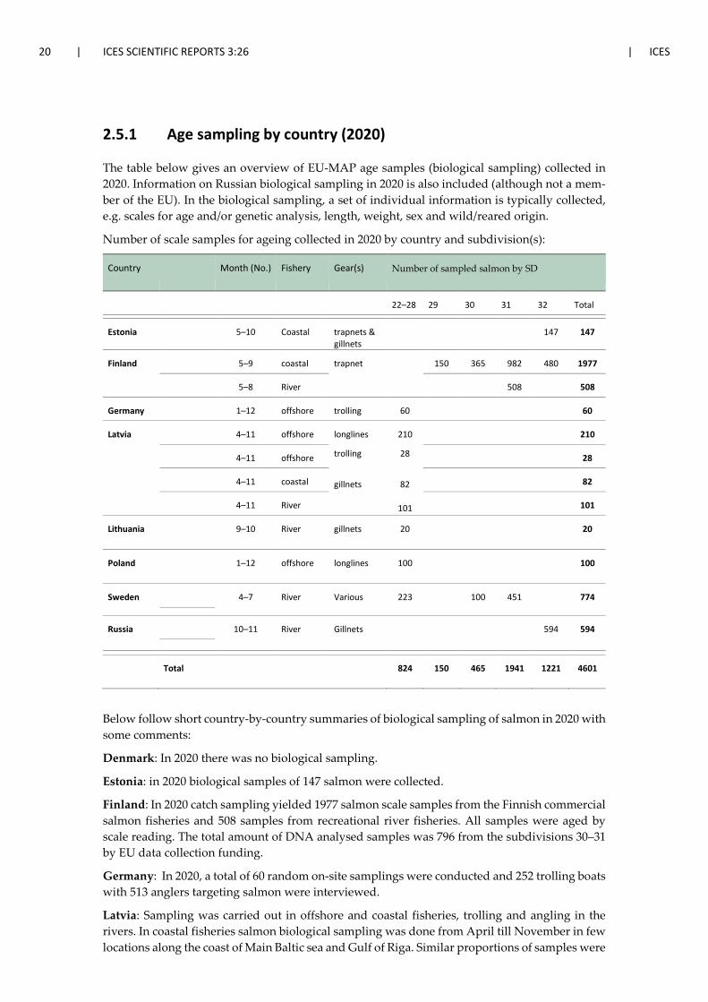
20 | ICES SCIENTIFIC REPORTS 3:26 | ICES
2.5.1 Age sampling by country (2020)
The table below gives an overview of EU-MAP age samples (biological sampling) collected in 2020. Information on Russian biological sampling in 2020 is also included (although not a mem-ber of the EU). In the biological sampling, a set of individual information is typically collected, e.g. scales for age and/or genetic analysis, length, weight, sex and wild/reared origin.
Number of scale samples for ageing collected in 2020 by country and subdivision(s):
Country Month (No.) Fishery Gear(s) Number of sampled salmon by SD
22–28 29 30 31 32 Total
Estonia 5–10 Coastal trapnets & gillnets
147 147
Finland 5–9 coastal trapnet 150 365 982 480 1977
5–8 River 508 508
Germany 1–12 offshore trolling 60 60
Latvia 4–11 offshore longlines
trolling
gillnets
210
28
82
101
210
4–11 offshore 28
4–11 coastal 82
4–11 River 101
Lithuania 9–10 River gillnets 20
20
Poland 1–12 offshore longlines 100 100
Sweden 4–7 River Various 223
100 451
774
Russia 10–11 River Gillnets
594 594
Total 824 150 465 1941 1221 4601
Below follow short country-by-country summaries of biological sampling of salmon in 2020 with some comments:
Denmark: In 2020 there was no biological sampling.
Estonia: in 2020 biological samples of 147 salmon were collected.
Finland: In 2020 catch sampling yielded 1977 salmon scale samples from the Finnish commercial salmon fisheries and 508 samples from recreational river fisheries. All samples were aged by scale reading. The total amount of DNA analysed samples was 796 from the subdivisions 30–31 by EU data collection funding.
Germany: In 2020, a total of 60 random on-site samplings were conducted and 252 trolling boats with 513 anglers targeting salmon were interviewed.
Latvia: Sampling was carried out in offshore and coastal fisheries, trolling and angling in the rivers. In coastal fisheries salmon biological sampling was done from April till November in few locations along the coast of Main Baltic sea and Gulf of Riga. Similar proportions of samples were
ICES | WGBAST 2021 | 21
collected at gillnet fishery at coast of Main Baltic and east coast of Gulf of Riga. 210 salmon sam-pled in offshore fishery with longlines (SD 28), 28 salmon sampled in offshore trolling. 98 salmon kelts were sampled in licensed angling in Salaca river and 3 in the Gauja river. All fish were aged by scale reading; in total 421 adult salmon.
Lithuania: Data of 20 migrating adult salmon caught in the Curonian lagoon analyzed.
Poland: There was only one sampling from catch on-board and two sampling from landings in 2020. The reason of that was significant harsh weather limiting number of fishing days. In addi-tion, a new sampling plan was implemented by Poland, starting from 2017/2018, in order to move gradually from metier based and purely opportunistic sampling towards the plan based on sta-tistics, with the aim to reach statistically sound sampling scheme (4S) in two–three years’ time. New sampling system provided high level of non-responses and refusals to take observers onboard. In addition, COVID-19 issue reduced the fishing effort in a spring time.
Russia: There is no ongoing biological sampling program running in Russia. Despite this, 594 salmon were collected and sampled for age, length and weight from brood stock fishing in 2020. Since Russia is not an EU Member State, the country is not obliged to follow EU regulations.
Sweden: Age sampling of smolts in rivers is included in the Swedish EU-MAP work plan. These data are needed in the WGBAST assessment modelling work; hence, the sampling is motivated on the ground of end-user needs. In 2020, a total of 774 smolt were sampled for age: 223 in Mör-rumsån (that flows into SD 25); 100 in Testeboån (SD 30) plus 315 in Ume/Vindelälven and 136 in Åbyälven (i.e. 451 altogether in SD 31).
2.5.2 Growth of salmon
Below a short summary of an ongoing study on growth of Baltic salmon in relation to composi-tion of the overall fish community is presented.
The average weight of salmon by age group increased around year 1990, simultaneously with an increase in sprat abundance (Figure 2.5.2.1). Despite some annual variation, the level of growth has remained rather stable. In 2016–2020, catch samples indicate a slight increase in mean weights by age (particularly in the MSW are groups) which is potentially a result of improved feeding conditions. Despite that salmon shares feeding areas with cod in the southern Baltic Main Basin, there is no clear reduction in the growth rate of salmon as has been observed for cod. The estimated post-smolt survival decreased strongly from the mid-1990s until 2005 (Figure 4.2.3.1) but this cannot be recognised in the growth data. Mortality mechanisms seem to affect salmon populations in such a way that survived individuals grow approximately as large in periods of high mortality as in periods of low mortality.
2.6 Genetic composition of Baltic salmon catches
In this section, results from recent analyses of stock proportions in catches are presented. De-scription of the genetic methodology used and how results are applied can be found in the Stock Annex (Annex 2).
2.6.1 Salmon stock and stock group proportions in Baltic salmon catches in the Bothnian Bay based on DNA microsatellite and freshwater age information
Combined DNA and smolt-age data have been used to estimate stock and stock group propor-tions of salmon catches in the Baltic Sea with a Bayesian method since the year 2000 (Pella and
22 | ICES SCIENTIFIC REPORTS 3:26 | ICES
Masuda, 2001; Koljonen, 2006; ICES, 2019). In 2020, Finnish coastal salmon catches from the Gulf of Bothnia were analysed from three fishing zones with temporal regulation of opening days. The regulation of the Finnish salmon fishing in the Gulf of Bothnia was changed in 2017, making it possible to start the fishing earlier (advanced starting date) than in previous years. To provide comparable data for the time-series from previous years, the estimates of stock and stock group proportions in the salmon catches from the fishing regulation zones were analyzed separately for catches preceding and succeeding the pre-2017 opening dates of the temporal regulation (Salmon fishing opening dates in 2016 were: Bothnian Sea: 10.6., the Quark area: 15.6., Bothnian Bay: 20.6., and the northernmost Bothnian Bay: 25.6.).
Methods The salmon river stock genotype baseline data used for the 2019 catches were also used for anal-ysis of the 2020 catch samples (Table 2.6.1, Figure 2.6.1) (ICES, 2020a). The current baseline river stock data set includes information on 17 DNA microsatellite loci from 39 Baltic salmon stocks from six countries, totalling 4453 individuals (Table 2.6.1).
As the temporal fishing regulation in the Gulf of Bothnia in Finland was changed in 2017, two separate collections of samples have been carried out since. In 2020, one sample (N=444) was collected from the late period, corresponding to the fishing period before the changed regula-tions in 2017. Another sample (N=352) was from the advanced season, early summer catches in 2020. Both samples were taken from three out of the four fishing zones (Bothnian Sea, the Quark area, Bothnian Bay and Northern Bothnian Bay). In all, scales from 796 salmon were analysed from the catches to produce the stock and stock group estimates.
Because smolt-age information was used for stock proportion estimation, the fish in the catch samples were divided into two smolt-age classes according to the smolt-age information from scale reading: 1–2 year old smolts and 3–5 year old smolts. As all released hatchery smolts are younger than three years, salmon in catch samples with a smolt age of older than two years originated presumably, or a priori, from the wild stocks, whereas individuals with a smolt age of one or two years could have originated either from a wild or a reared stock. The same assump-tion is used in scale reading as well, when differentiating wild and reared fish. Correspondingly, smolt-age distributions were needed for all baseline stocks in addition to genetic data (Table 2.6.2). Smolt age distributions of wild smolts in Tornionjoki, Simojoki, Kalixälven and Råneälven were updated to represent the smolt-age distributions of smolt year classes from 2017 to 2019, of which the catches of adult salmon in 2020 were mainly composed. For the other stocks an average of smolt ages over the years was used (Table 2.6.2).
Results In the Finnish Bothnian Bay salmon catch samples from the latter part of the summer fishing season (comparable to time of sampling in the years before 2017), the proportion of wild stocks was the lowest since 2009 (58% PI: 53–63%) (Table 2.6.3). The proportion of wild fish was about 70% in 2015 and 2016, and even 80% in the maximum year of 2014. The number of hatchery-released fish among smolts has been fairly constant over time, so it can be assumed that the number of wild salmon has decreased in the catches in 2020 compared to the 2018–2019 level, back to the level of the weak years of 2012, 2013 and 2017 (Figure 2.6.2).
During the advanced fishing season in 2020, the proportion of wild fish was about 15 percentage points higher, about 73% (PI: 68–78 %), than during the late fishing season (58% PI: 53–63%) (Table 2.6.3) (Figure 2.6.2). The difference in stock composition between early and late fishing seasons was larger in 2020 than in 2019, similar to the difference in stock composition in 2017 and 2018 (Table 2.6.3) (Figure 2.6.2). The share of hatchery fish increased during the early season. It seems that in the years, when the number of returning wild spawners is low, the difference between early and late season is larger. When there are less wild spawners to return, the catches
ICES | WGBAST 2021 | 23
of the late fishing season include more hatchery fish. The difference between the seasons in-creases when the number of returning spawners is low. When there are more wild born fish returning, their share in the latter season catches increases as well.
Focusing only on the four years when the early season fishing was allowed (2017–2020), the dif-ference between the wild stock group proportions during the early (77%) and late season (65%) fisheries was still on average 12 percentage points (Table 2.6.4.). The difference is clearest in the northernmost area of the Bothnian Bay, where in the advanced fishing season, from June 9th to June 24th, the proportion of wild stocks, pooled over four years, was 78%, decreasing after the early fishing season to 61%. In the Bothnian Sea catches, the proportion of wild stocks was more constant, and the differences in wild stock proportions between the advanced and late seasons were smaller than in the Bothnian Bay catches (Table 2.6.4) (Figure 2.6.3). The differences be-tween wild stock group proportions in the early and late seasons were also smaller in the Quark (Table 2.6.4, Figure 2.6.3). There were only few individual Swedish hatchery fish (< 1%) in the advanced fishing season catches, while their proportion in the later season was 7%, which also indicates the different migration timing tendencies of wild and reared stock groups.
The individual river stock proportions in the 2020 salmon catches during the late season were very near to the long term (2013–2020) total proportions (Table 2.6.5). The most common stock was the wild born Tornionjoki salmon (40%), the next common were hatchery origin salmon from Tornionjoki (14%), Kalixälven (13%), and Iijoki (12%). When stock proportions of early and late fishing seasons were compared the clearest difference was in the proportions of Kalixälven salmon: 22% in the early season, 13% in the late season (Figure 2.6.4.). Kalixälven salmon seem to leave the Finnish coast early, while the wild Tornionjoki salmon remain to be caught also in the late season. During the early, advanced fishing season, the stock composition of the catches was relatively homogenous in all three fishing zones (Table 2.6.6). Iijoki salmon were less com-mon in the northernmost area than in the southern zones. During the late season Iijoki salmon were less common (9%) in the Bothnian Sea catches than in the more northern zones (15–18%), and Kalixälven salmon less common (8%) in the most northern area, than in the more southern zones (15–19%) (Table 2.6.6). Early season fishery is targeting relatively more the wild-born salmon.
2.7 Management measures influencing the salmon fishery
2.7.1 International regulatory measures
Detailed information and evaluations of international regulatory measures are presented in the Stock Annex (Annex 2).
Exemption from landing obligation. In 2014, the European Commission decided to introduce a discard ban for commercial fisheries, covering all species under TACs (Commission Delegated Regulation (EU) No 1396/2014 of 20 October 2014). Salmon fisheries in the Baltic Sea have an exemption from the landing obligation for salmon caught with trapnets, creels/pots, fykenets and poundnets (see Annex 2 for more details). The exemption for salmon fisheries using partic-ular gears, is based on the assumption that fish caught in these gears has a high likelihood of survival after capture, handling and release (Commission delegated regulation (EU) 2018/211). However, at that time, information about survival rates of released salmon caught in the Baltic Sea commercial fishery, particularly in the most commonly used pontoon/pushup traps, was rather limited.
A review of recent studies carried out in the Baltic Sea (Östergren et al., 2020) indicate that discard mortality in the Baltic salmon coastal fishery is strongly dependent on the type of gear used, as well as emptying procedures and handling time. In addition, external factors, in particular high
24 | ICES SCIENTIFIC REPORTS 3:26 | ICES
water temperature and poor health status of the fish, may have a large negative impact on post-release survival. In the studies reviewed by Östergren et al. (2020), total discard mortality of salmon caught in pontoon traps varied between studies in the range of 47–88% when the gear was emptied using the traditional technique. These estimates include both immediate mortality, and subsequent post-release mortality (usually only estimated for shorter periods). Recent stud-ies also show that the mortality could be reduced by using emptying procedures where the fish is handled more gently. When a net bag, in Swedish “Vittjanpåse”, was attached to Pontoon traps, the total discard mortality was reduced to 17–63%.
The current exemption from the landing obligation for Baltic salmon fisheries will cease to apply on 31 December 2020. Whether there will be a continued exemption from 2021 and onwards will be handled by BALTFISH, STECF and EU COM during spring and summer 2020.
2.7.2 National regulatory measures
National regulatory measures are, unlike the international regulatory measures, updated more often, at times on a yearly basis, and therefore they are presented here and not in the Stock An-nex. Effects of national regulatory measures on stock development are generally not evaluated by WGBAST.
In Denmark, no new national regulatory measures were implemented in 2020. According to reg-ulations for the period 2014–2020 (BEK nr 212 af 01/03/2017 - Bekendtgørelse om regulering af fiskeriet i 2014–2020) the following rules must be followed:
• All commercial vessels fishing salmon must be registered as salmon fishing boats and have a specific permission for the fishery.
• Discard is not allowed, but seal damaged salmon can be discarded without deduction from the quota.
• Vessels with a catch of ten or more salmon must notify the Fisheries Inspection before entering the harbour.
For recreational trolling fisheries no national legislation is in practice. However, voluntary re-strictions are recommended by angler association(s).
Further restrictions: Throughout the year, all streams with outlets wider than 2 m are protected by closed areas within 500 m from the mouth. Otherwise, the closure period is four months at the time of spawning run. Estuaries are usually protected by an extended zone. Gillnetting is not permitted within 100 m of the low waterline. A closed period for salmon (and sea trout) has been established from 16th of November to 15th of January in freshwater. In the sea, this only applies for sexually mature fish in spawning dress (coloured). A maximum of three gillnets and three fykenets/sets of hooks are allowed per fisherman.
Around Bornholm, a maximum of six sets of gear (nets or hooks) are permitted per fisherman. Fishing with hooks is permitted only between 1st of October–1st of May. For each set of hooks, a maximum of 100 hooks is allowed. Maximum length of the six nets allowed is 270 m in total. Between 16th September and the last day in February nets may be combined as follows, either: (A) up to six bottom gillnets, or (B) up to five bottom gillnets and one floating net (maximum 45 m length, maximum height 3 m, minimum mesh size (total) 157 mm (called ‘Salmon nets’) OR five bottom gillnets and one floating net 45 m length and height 12 m with minimum mesh size (total) 57 mm (called ‘Bornholmer nets’), or (C) up to four bottom gillnets and one floating gillnet maximum 45 length and 3 m height, and one ‘salmon net’. Between 1st of March and 15th of September, maximum three of the six gillnets allowed can be floating (maximum length 135 m).
Further restrictions around Bornholm: On water with less than 30 m depth: a maximum of three gillnets is allowed (all year). Use of floating gillnets is prohibited from 16 September to the last
ICES | WGBAST 2021 | 25
day of February. Between 1st of March and 30th of April, maximum mesh size (total) is 60 mm in floating gillnets. All year, the use of both ‘Bornholmer nets’ and ‘Salmon nets’ is prohibited. On water with more than 30 m depth: use of ‘Bornholmer nets’ is prohibited between 1st of December and 31st of May. All year only one ‘Salmon net’ is permitted. Harvest of sea trout is limited to maximum three fish per man per day (and maximum three per boat per day). No mandatory bag limit exists for salmon, though local trolling fishers have agreed to harvest maximum two salmon per fisher per day, minimum length 75 cm and preferably retain only released (fin-clipped) salmon.
In Estonia salmon offshore fishery is regulated by EC regulations, coastal and river fishery also by national rules. No new fishing restrictions was established in 2020. There last new national regulatory measures were implemented in 2019 concerning the recreational sector.
• In river Pühajõgi, Loobu, Selja, Pirita, Vääna and Purtse recreational fishery for salmon and sea trout is closed from 20th of October–30th of November.
• Recreational salmon fishing was banned in Valgejõgi.
In general, since 2011, the following restrictions are in practice:
• no commercial fishery in salmon (and sea trout) spawning rivers is permitted, with the exception of lamprey fishing;
• only licensed angling is permitted.
Some specific management regulations are also in place on a river basis regarding closure peri-ods for angling. A closed period for salmon (and sea trout) angling is established in rivers Narva, Purtse, Kunda, Selja Loobu, Valgejõgi, Jägala, Pirita, Keila, Vasalemma, and Pärnu from 1 Sep-tember–30 November, and in other rivers from 1 September–31 October. Exceptions for these closures are allowed by decree of the Minister of Environment in rivers with a reared (Narva) or mixed salmon stock (Purtse, Selja, Valgejõgi, Jägala, Pirita and Vääna). Below of dams and wa-terfalls, all kind of fishing is prohibited at a distance of 100 m. In the River Pärnu, below Sindi dam, this distance is 500 m.
Furthermore, there is an all-year-round closed area of 1000 m radius at the river mouths of the present or potential salmon spawning rivers Purtse, Kunda, Selja, Loobu, Valgejõgi, Jägala, Pi-rita, Keila, and Vasalemma, and at the river mouths of the sea trout spawning rivers Punapea, Õngu, and Pidula. Since 2011, the closed area for fishing around the river mouth was extended from 1000–1500 m for the time period 1 September–31 October for rivers Kunda, Selja, Loobu, Valgejõe, Pirita, Keila, Vääna, Vasalemma and Purtse. In rivers Selja, Valgejõgi, Pirita, Vääna and Purtse, recreational fishery for salmon (and sea trout) is banned from 15 October to 15 November. In the case of the most important Estonian sea trout spawning rivers (Pada, Toolse, Vainupea, Mustoja, Altja, Võsu, Pudisoo, Loo, Vääna, Vihterpadu, Nõva, Riguldi, Kolga, Rannametsa, Va-najõgi, Jämaja) a closed area of 500 m is established from 15th of August to 1st of December. In most of the salmon (and sea trout) rivers, angling with natural bait is prohibited.
In Finland, in the Main Basin salmon fishing has been forbidden for the Finnish vessels from year 2013. Coastal salmon fishing regulation for the Gulf of Bothnia was renewed in 2017. Also, individual quota system was implemented in salmon fishery (and as well as Baltic herring and sprat fishery) in 2017. In Åland Islands prevails a separate regulation.
In the Gulf of Bothnia for commercial fisherman salmon fishing is allowed to start with one trap-net in the following dates in four zones: Bothnian Sea (59°00’N–62°30’N) May 1st, Quark (62°30’N–64°N) May 6th, Southern Bothnian Bay (64°00’N–65°30’N) May 11th and Northern Bot-nian Bay (65°30’N–->) May 16th. They can set one more trapnet for fishing in the following dates: Bothnian Sea (59°00’N–62°30’N) June 10th, Quark (62°30’N–64°N) June 15th, Southern Bothnian Bay (64°00’N–65°30’N) June 20th and Northern Bothnian Bay (65°30’N–>) June 25th. After one
26 | ICES SCIENTIFIC REPORTS 3:26 | ICES
week from these two, more trapnets are allowed to set for fishing (maximum a total of four trap-nets per fisherman).
Also, in terminal fishing areas, the number of trapnets and fishing period was restricted. Earlier in terminal fishing areas the number of trapnets was unlimited and only in Kemi terminal area there was a closure in the early summer. Now the regulation in terminal areas is more similar to the rest of the region. Fishing with one trapnet is allowed to start at the same time as outside the areas, but the number of trapnets can be raised up to three on June 17th and up to eight on June 25th (for fishers with turnover less than equal to 10 000 € up to two and four for respectively).
In the area outside of River Simojoki, salmon fishing may start on July 16th and outside the mouth of river Tornionjoki on June 17th.
All salmon have to be marked with a coded landing mark. In the first period of the season (when one trapnet is allowed) fisher is allowed to utilize of 25% his/her individual quota at maximum. Large trapnets (higher than 1.5 m) are allowed only for commercial fishers.
Salmon fishing with longlines and gillnets is forbidden in the Archipelago Sea and Gulf of Both-nia from April 1st to June 16th–July 1st depending on the area.
In Germany, no new national regulatory measures were implemented in 2020. For several years, there is no quota allocated in the commercial sector, i.e. there is no directed commercial salmon fishery anymore. There are two federal states bordering the Baltic coast: Schleswig-Holstein, (SH) and Mecklenburg-Western Pomerania (MV). Commercial (coastal) fishing and recreational fishing is under the jurisdiction of the German federal states. Consequently, marine coastal fish-ing is managed with different legislation. The fishing season is closed both for commercial and recreational fisheries during autumn, in SH 1st of October–31st of December (only coloured fish) and in MV 15th of September–14th of December. Closed areas in both federal states include pro-tected spawning grounds in coastal waters, 300–400 m around spawning streams/rivers. For commercial fisheries there is also a 200 m gillnet ban in front of the coastline. In MV, trolling fisheries is permitted at a distance >1 km from the coastline between September 15th and March 15th and there is a rod limit of three rods per angler in place. In MV, there is also a bag limit in place allowing landing of three salmonids (sea trout or salmon) per day and angler. Recreational fishery for salmon (and sea trout) is allowed on a licence basis. The minimum landing size is 60 cm in both states.
In Latvia in 2020, licensed angling for descending hatchery origin (finclipped) sea trout and salmon kelts was opened also in Gauja river. Similar to the regulations established in Salaca and Venta river, daily bag limit is one sea trout or salmon.
In summary, current national legislation in commercial offshore and in coastal waters includes the following restrictions:
• In the Gulf of Riga, salmon driftnet and longline fishing is not permitted; • In coastal waters, salmon fishing is prohibited from 1st of October–15th November; • Salmon fishing in coastal waters has been restricted indirectly, by limiting the number of
gears in the fishing season.
In the recreational trolling fishery, one person is allowed to use a maximum number of three fishing rods in the waters of the Baltic Sea and the Gulf of Riga, if each gear has no more than three hooks of any type (including treble hooks), and where more than one treble-hook hook is allowed only if it is free (moving) attached to one artificial bait. It is prohibited to use natural bait for salmon and trout. Daily bag limit is one salmon and one sea trout per person. Minimum size limit is 60 cm for salmon and 50 cm for sea trout.

ICES | WGBAST 2021 | 27
In the rivers with natural reproduction of salmon, all angling and fishing for salmon and sea trout is prohibited with exception of licensed angling for sea trout and salmon during the spring season in the rivers Salaca and Venta. Daily bag limit is one sea trout or one salmon. Since 2013, all gillnetting is prohibited all year round in a 3 km zone around the River Salaca outlet. In 2004, the restriction zones were enlarged from 1 to 2 km for the rivers Gauja and Venta. In rivers Dau-gava and Bullupe (connects rivers Lielupe and Daugava) angling and commercial fishing of salmon is allowed since 2007. However, it is prohibited to use gillnets in these rivers.
In Lithuania salmon offshore fishery is regulated by EC regulations, coastal and river fishery also by national rules. Most regulatory measures is as it was in previous years. It is some changes for fishing zones in Nemunas river and new requirement for commercial fishery in Curonian lagoon; all (dead or alive) salmon and sea trout caught with fykenets must be released.
The commercial fishery is regulated during time of salmon (and sea trout) migration in the Klaipėda Strait and the Curonian lagoon. Fishing is prohibited all year-round in a predefined part of the Klaipėda strait. From the 1st of September–31st of October, during the salmon (and sea trout) migration, fishing with nets is prohibited on the eastern stretch of the Curonian lagoon between Klaipėda and Skirvytė, at a 2 km distance from the eastern shore.
Recreational salmon (and sea trout) fisheries along the coast are regulated by one set of rules, whereas in inland waters another set of rules regulates the fisheries. For recreational fishing of salmon (and sea trout) in the Baltic Sea, one either needs to buy a fishing ticket or be entitled to special fishing rights to fish. In inland waters, you need a recreational fishing card for fishing. Both in the sea and in inland waters, there is a bag limit of one salmon or sea trout per angler and fishing day. In inland waters, the minimum size has been extended to 65 cm.
In the period September 15th to 31st of October, recreational fishing is prohibited within a 0.5 km radius from the Šventoji and Rėkstyne river mouths, and from the southern and northern break-waters of Klaipėda Strait. During the same period, commercial fishing is prohibited within a 0.5 km radius from Šventoji River mouth, and 3 km from the Curonian lagoon and Baltic Sea confluence. From 1st of October to 31st of December, all types of fishing are prohibited in 161 streams, because of brown trout and sea trout spawning.
In larger rivers, such as Neris and Šventoji (with twelve rivers/tributaries in total), special pro-tected zones have been selected where schooling of salmon and sea trout occurs. In these selected zones, licensed fishing is only permitted from 16th of September until 15th of October. Last year, the angling of salmon and sea trout in this selected river zones was limited by a ‘catch and re-lease’ rule (from 1st until 15th October). From 16th of October to 31st of December any kind of fishing is prohibited in these areas. From 1st of January, licensed salmon (and sea trout) kelt fishing is permitted in the Minija, Veiviržas, Skirvytė, Jūra, Atmata, Nemunas, Neris, Dubysa, Siesartis and Šventoji river. Fishing with a licence is allowed from 1st of January to 1st of October in designated stretches of the listed rivers. In the inland waters, regulation of fishing is more complex. In case of retaining a salmon (or sea trout), a specific part of the recreational fishing card must be removed not later than within five minutes. Such a marked recreational fishing card means that you are not allowed to continue fishing there and then.
In Poland one national regulatory measure was implemented in 2020: the protective period for salmon and sea trout for recreational fisheries have been shortened compared to the previous one (was: ‘between 15th September and 30th November’) to the period 'between 15th September and 15th November beyond four nautical miles from the shore'. That regulation has been imple-mented to unify the legal acts related to the protective period for salmon and sea trout, however, the shortened protective period has been chosen.
In addition to EC measures, seasonal closures and fixed protected areas are in force within terri-torial waters managed by Regional Fisheries Inspectorates. Fishing for salmon (and sea trout) in
28 | ICES SCIENTIFIC REPORTS 3:26 | ICES
the sea is not allowed between 15th of September and 15th of November within a predefined belt along the coastal zone (<4 Nm). A new law for recreational salmon fishing in Polish EEZ was introduced in 2015 including:
• catch quotas (per day/per angler); • minimum size limits (TL.); • periods and areas for protected fish species; • minimum distance between anglers.
Rod fishing (coastal fishing, boat/belly boat fishing, and organized cruises on board fishing ves-sels) and spear fishing is allowed. Recreational fishing with nets is not allowed. A new system of obtaining fishing licences has been established. Currently, proof of a bank transfer with spec-ified personal information is needed for legal fishing. The permit can be issued for a period of one week, one month or one year.
Since 2005, commercial fisheries for salmon (and sea trout) in rivers is based on new imple-mented rules. Fisheries opportunities were sold in 2005 by the state on a tender basis, where the bidder had to submit a fishing ten-year operational plan including restocking. Commercial river fisheries directed for sea trout and salmon already exist almost only in the Vistula River. How-ever, salmon are rare. In Pomeranian rivers, some salmon are collected annually for brood stock during spawning run.
In the rivers, angling for salmon and sea trout is forbidden between 1st of October and 31st of December. A fishing licence and permit are needed for fishing in the rivers. Only rod fishing is allowed for fishing for salmon and sea trout in the rivers. In addition, in Rivers Ina, Rega, Parsęta and Słupia, anglers must release all salmon that have been caught.
In Russia, no changes in the national regulations have been implemented since 2001. The inter-national fishery rules are extended to the coastline. In all rivers, and within one nautical mile of their mouths, fishing and angling for salmon is prohibited during all year, except fishing for brood stock for hatcheries.
In Sweden, for the commercial fisheries in 2020, as in recent years, the Swedish salmon quota was allocated to the coastal fishery as the Swedish offshore fishery targeting salmon and sea trout was phased out in 2012–2013. Management measures for salmon include an early summer ban and a minimum landing size of 60 cm. The aim of the early summer ban in the coastal fishery is to ensure that part of the migrating population of adult salmon ascend rivers before the fishing season starts. Starting dates of the Swedish commercial coastal fishing season in 2020 were the same as in 2019. North of latitude 62º55’N the fishing season started 17 June except in the pro-tection area outside River Umeälven where the starting date was set to 1 July. Exemptions from the seasonal regulation of the salmon fishery was allowed by the local county board to profes-sional fishermen in the area north of latitude 62º55’N up to the border between the counties Väs-terbotten and Norrbotten (except the protection area outside Umeälven), so that a limited fishery could start 12 June. South of latitude 62º55’N, commercial coastal fishing in 2020 was allowed from 1 April.
Salmon fishing opportunities for Swedish commercial fishermen in 2020 amounted to 26 991 salmon and consisted of the 2020 quota of 24 252 salmon plus an unutilized part (2739 salmon) of the 2019 quota. Of the 26 991 salmon, 591 were reserved for bycatches in fisheries targeting other species and as a buffer if catches would exceed the quota. 26 400 salmon were allocated to the commercial coastal fishery and were divided between ICES subdivisions (SD) in a similar way as in the last few years. In SD 31 the regional quota was set to 19 200 salmon. Among those, 2000 salmon were allocated specifically to the protection area outside River Umeälven, where fishing started 1 July. The aim of the changed regulations outside Umeälven was to protect the
ICES | WGBAST 2021 | 29
(early migrating) weak wild salmon population in the tributary Vindelälven during the spawn-ing migration. In SD 30, the regional quota was set to 7000 salmon. In SD 22–29 the regional quota was set to 200 salmon because of the higher expected proportion of salmon from weaker popu-lations in these catches (as compared to SD 30 and 31). According to the latest information, com-mercial catches in 2020 were below regional quotas in all three areas (landed share of quota was 68%, 71% and 95% in SD 22–29, SD 30 and SD 31, respectively). The total Swedish coastal catch in 2020 in SD 22–31 (23 292 salmon) corresponded to 88% of the total Swedish quota for the coastal fishery in these three areas (26 400 salmon).
Recreational fisheries in the sea and in rivers are also managed through national regulations. Recreational coastal fisheries with trap nets in the counties of Norrbotten, Västerbotten and part of Västernorrland were, as in latest years, allowed from 1 July until the quota of salmon within the commercial fishery was fulfilled. In SD 31, the salmon fishery was stopped 5 July 2020 when the regional salmon quota was filled. Hence, it was possible to conduct recreational fishing with trapnets in SD 31 between 1 and 4 July, but the recreational fishery using these gears is most likely very small or non-existent due to the ban for recreational fishermen in the Baltic Sea to sell their catches; many recreational trapnet fishermen have applied for a commercial licence and their catches are now included in the quota. The recreational fishery using trapnets in SD 30 is likely also small or non-existent. SLU Aqua plan to carry out an inventory of the recreational coastal fishery for salmon during 2021.
Since 2013, Swedish offshore trolling fisheries (that mainly takes place in the Main Basin) are only allowed to land salmon without an adipose fin (i.e. finclipped reared salmon). In all rivers there is a general bag limit of one salmon and one trout per fisherman and day. Also fishing periods are regulated on a national level. In Gulf of Bothnian wild rivers, for example, angling for salmon is forbidden from 1 September until 31 December, and in some rivers, angling is also forbidden between 1 May and 18 June. In 2019, new regulations were introduced in Vindelälven and Ljungan, including a maximum size limit of 65 cm in Vindelälven and a total ban for catching salmon in Ljungan. These restrictions were introduced to protect the weak wild salmon popula-tions is these rivers. In addition to national regulations, local fishing and management organiza-tions may stipulate more restrictive rules.
The management of fisheries in the boarder river Torneälven, including the coastal area directly outside the river mouth, is handled through an agreement between Sweden and Finland. The Swedish-Finnish agreement includes for example a specified time period within which the com-mercial coastal fishery in the river mouth is allowed to start. Regulations targeting the river fish-ery are also handled in the agreement. Deviations from the agreed fishing regulations in this area are negotiated and decided upon on an annual basis by SwAM (according to a Government com-mission from the Swedish Ministry of Enterprise and Innovation) and the Finnish Ministry of Agriculture and Forestry.
In order to improve the situation for weak sea trout stocks in SD 31, a number of changes have been implemented in recent years. The minimum size for landed sea trout was raised from 40 to 50 cm in the sea 1 July 2006. Furthermore, a ban of fishing with nets in areas with a depth of less than 3 meters during the period 1 April–10 June and 1 October–31 December was implemented in 2006 to decrease bycatch of trout in fisheries targeting other species. Further restrictions for rivers in Bothnian Bay (SD 31) were adopted in 2013, including shortening of the autumn period for fishing with two weeks, restrictions of catch size (window size 30–45 cm), and landing of only one trout per fisherman and day. In River Torneälven, sea trout fishing is forbidden. From 1 September 2019, new fishing regulations were introduced in SD 30 to improve the situation for coastal fish populations in this area. These regulations include a ban for fishing with nets in areas with less than 3 meters depth between 1 September and 10 June, a complete net ban between 15 October and 30 November, increase of the minimum size for sea trout from 40 to 50 cm, and a daily bag limit of one wild sea trout when fishing with sport fishing equipment or fykenets. In
30 | ICES SCIENTIFIC REPORTS 3:26 | ICES
April 2021, a daily bag limit of one wild sea trout when fishing with sport fishing equipment or fykenets was introduced also along the Swedish southeast coast (SD 27–29). The new regulations implemented in 2021 also include a few new protection areas along the southeast coast to protect sea trout during the autumn migration.
In 2020, the Swedish Agency for Marine and Water Management initiated an overview of the fishing regulations in both rivers and coastal areas (see Kagervall et al., 2020; Magnusson et al., 2020; Dannewitz et al., 2020 a, b). This process will likely result in updated regulations/re-strictions in the coming years. The aim of the overview is to develop the fishery management to become more stock-specific so that fishing possibilities will be adapted to the status of individual river stocks of salmon and sea trout, and also the situation for other migrating and coastal fish species.
A discard ban for quota-regulated species in the Baltic Sea was implemented by EU 1 January 2015. All salmon and other quota-regulated species caught in fisheries targeting salmon should be landed and registered. Likewise, all salmon taken as bycatch in fisheries targeting other spe-cies should be landed and registered. Salmon fisheries in the Baltic Sea have had an exemption from the landing obligation for salmon caught with trapnets, creels/pots, fykenets and pound-nets. An exemption makes it possible to release wild salmon back into the sea, as a measure to steer the exploitation towards reared (finclipped) salmon. The possibility to release salmon also makes it possible to catch other species outside the salmon fishing season or when the salmon quota is filled. The exemption from the landing obligation ceased to apply 31 December 2020, and at the time of writing it is unclear whether a new exemption will be decided by EU later this spring or not.
The earlier exemption was based on the assumption that salmon has a high likelihood of survival after capture, handling and release. The knowledge about long-term survival of salmon after release is, however, limited. A review of studies on the subject (Östergren et al., 2020), including results from recent studies in Sweden, indicates that the discard mortality in the Baltic salmon coastal fishery is strongly dependent on the type of gear used, as well as handling time and emptying procedures. Baltic salmon captured in the most common gear type (the pontoon trap) typically show physical injuries (e.g. blood in eyes, scale losses) which together with physiolog-ical stress increases the risk of discard mortality. In addition, extrinsic factors, in particular high water temperature and poor health, may have a large negative impact on post-release survival. With a modified design of the Pontoon trap, where a net bag (“Vittjanpåse”) is attached to the trap, which facilitates gentle handling of the fish, the total discard mortality can be reduced sub-stantially given that the fish are correctly/gently handled.
Member States around the Baltic Sea have, through BALTFISH, produced a Joint recommenda-tion regarding a new discard plan for Baltic salmon and an exemption from the landing obliga-tion for certain fishing gears. The pontoon trap is suggested to be included among gears ex-empted from the landing obligation only if a “vittjanpåse” is attached to the trap, thereby facili-tating gentle handling of the fish. As indicated above, however, EU has not yet taken any deci-sion regarding a new discard plan for Baltic salmon. A landing obligation that would involve also trapnet fisheries would most likely affect the exploitation pattern of both salmon and other species. The estimated share of undersized salmon in coastal fisheries with traps is low, so a discard ban will not have any major impacts on the fishery targeting salmon. However, the pos-sibility of releasing wild salmon back into the sea as a conservation measure to steer the exploi-tation towards reared (finclipped) salmon will disappear. Also, trapnet fisheries targeting other species may have to be more strongly regulated than today if salmon are taken as bycatch, which will probably have large economic consequences for fishermen in some areas. This effect may at least partly be overcome by the development of selective gears not catching salmon and/or redi-recting the fishery with trapnets for other species toward time periods when salmon are less frequent along the coast.
ICES | WGBAST 2021 | 31
2.8 Other factors influencing the salmon fishery
The incitement to fish salmon is (as for other species) influenced by a number of factors, such as the possibilities for selling the fish and then at which market prize, eventual opportunities to target and catch other species and problems with damages to the catches caused by seals and possibly birds.
Further, the possibilities for selling the fish is evidently affected by co-factors such as levels of contaminants, e.g. dioxin. Detailed information about dioxin contents in Baltic salmon, and how this affects the fishery, is presented in Stock Annex (Annex 2, Section A.2.6). Also, the overall health status of the fish is of importance. See Section 3.4.4 for a summary of disease problems seen in several rivers and areas in later years.
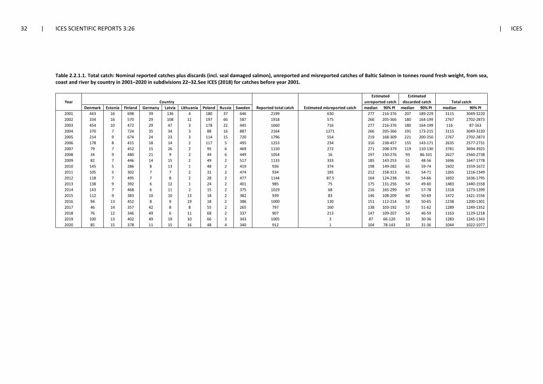
32 | ICES SCIENTIFIC REPORTS 3:26 | ICES
Table 2.2.1.1. Total catch: Nominal reported catches plus discards (incl. seal damaged salmon), unreported and misreported catches of Baltic Salmon in tonnes round fresh weight, from sea, coast and river by country in 2001–2020 in subdivisions 22–32.See ICES (2018) for catches before year 2001.
Year CountryDenmark Estonia Finland Germany Latvia Lithuania Poland Russia Sweden median 90% PI median 90% PI median 90% PI
2001 443 16 698 39 136 4 180 37 646 2199 630 277 216-376 207 189-229 3115 3049-32202002 334 16 570 29 108 11 197 66 587 1918 575 266 205-366 180 164-199 2767 2702-28732003 454 10 472 29 47 3 178 22 445 1660 716 277 216-376 180 164-199 116 87-1632004 370 7 724 35 34 3 88 16 887 2164 1271 266 205-366 191 173-215 3115 3049-32202005 214 9 674 24 23 3 114 15 720 1796 554 219 168-309 221 200-250 2767 2702-28732006 178 8 415 18 14 2 117 5 495 1253 234 316 238-457 155 143-171 2635 2577-27312007 79 7 452 15 26 2 95 6 469 1150 272 271 208-379 119 110-130 3781 3694-39252008 34 9 480 21 9 2 44 6 449 1054 16 197 150-276 93 86-101 2627 2560-27382009 82 7 446 14 15 2 49 2 517 1133 333 185 143-253 51 48-56 1696 1647-17782010 145 5 286 8 13 1 48 2 419 926 374 198 149-282 65 59-74 1602 1559-16722011 105 5 302 7 7 2 31 2 474 934 185 212 158-313 61 54-71 1265 1216-13492012 118 7 495 7 8 2 28 2 477 1144 87.5 164 124-238 59 54-66 1692 1636-17952013 138 9 392 6 12 1 24 2 401 985 75 175 131-256 54 49-60 1483 1440-15582014 143 7 468 6 11 2 15 2 375 1029 68 216 165-299 67 57-78 1318 1273-13992015 112 9 383 10 10 13 18 2 382 939 83 146 108-209 60 50-69 1472 1421-15562016 94 13 452 8 9 19 18 2 386 1000 130 151 112-214 58 50-65 1238 1200-13012017 46 14 357 42 8 8 55 2 265 797 160 138 103-192 57 51-62 1289 1249-13522018 76 12 346 49 6 11 68 2 337 907 213 147 109-207 54 46-59 1163 1129-12182019 100 13 402 49 19 10 66 3 343 1005 3 87 66-120 33 30-36 1283 1245-13432020 85 15 378 11 15 16 48 4 340 912 1 104 78-143 33 31-36 1044 1022-1077
Reported total catch Estimated misreported catch
Estimated unreported catch
Estimated discarded catch Total catch
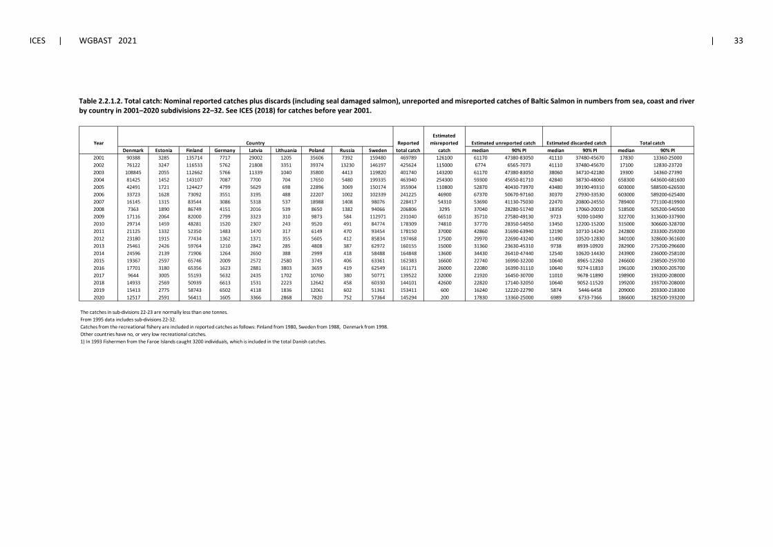
ICES | WGBAST 2021 | 33
Table 2.2.1.2. Total catch: Nominal reported catches plus discards (including seal damaged salmon), unreported and misreported catches of Baltic Salmon in numbers from sea, coast and river by country in 2001–2020 subdivisions 22–32. See ICES (2018) for catches before year 2001.
Year CountryDenmark Estonia Finland Germany Latvia Lithuania Poland Russia Sweden median 90% PI median 90% PI median 90% PI
2001 90388 3285 135714 7717 29002 1205 35606 7392 159480 469789 126100 61170 47380-83050 41110 37480-45670 17830 13360-250002002 76122 3247 116533 5762 21808 3351 39374 13230 146197 425624 115000 6774 6565-7073 41110 37480-45670 17100 12830-237202003 108845 2055 112662 5766 11339 1040 35800 4413 119820 401740 143200 61170 47380-83050 38060 34710-42180 19300 14360-273902004 81425 1452 143107 7087 7700 704 17650 5480 199335 463940 254300 59300 45650-81710 42840 38730-48060 658300 643600-6816002005 42491 1721 124427 4799 5629 698 22896 3069 150174 355904 110800 52870 40430-73970 43480 39190-49310 603000 588500-6265002006 33723 1628 73092 3551 3195 488 22207 1002 102339 241225 46900 67370 50670-97160 30370 27930-33530 603000 589200-6254002007 16145 1315 83544 3086 5318 537 18988 1408 98076 228417 54310 53690 41130-75030 22470 20800-24550 789400 771100-8199002008 7363 1890 86749 4151 2016 539 8650 1382 94066 206806 3295 37040 28280-51740 18350 17060-20010 518500 505200-5405002009 17116 2064 82000 2799 3323 310 9873 584 112971 231040 66510 35710 27580-49130 9723 9200-10490 322700 313600-3379002010 29714 1459 48281 1520 2307 243 9520 491 84774 178309 74810 37770 28350-54050 13450 12200-15200 315000 306600-3287002011 21125 1332 52350 1483 1470 317 6149 470 93454 178150 37000 42860 31690-63940 12190 10710-14240 242800 233300-2592002012 23180 1915 77434 1362 1371 355 5605 412 85834 197468 17500 29970 22690-43240 11490 10520-12830 340100 328600-3616002013 25461 2426 59764 1210 2842 285 4808 387 62972 160155 15000 31360 23630-45310 9738 8939-10920 282900 275200-2966002014 24596 2139 71906 1264 2650 388 2999 418 58488 164848 13600 34430 26410-47440 12540 10620-14430 243900 236000-2581002015 19367 2597 65746 2009 2572 2580 3745 406 63361 162383 16600 22740 16990-32200 10640 8965-12260 246600 238500-2597002016 17701 3180 65356 1623 2881 3803 3659 419 62549 161171 26000 22080 16390-31110 10640 9274-11810 196100 190300-2057002017 9644 3005 55193 5632 2435 1702 10760 380 50771 139522 32000 21920 16450-30700 11010 9678-11890 198900 193200-2080002018 14933 2569 50939 6613 1531 2223 12642 458 60330 144101 42600 22820 17140-32050 10640 9052-11520 199200 193700-2080002019 15413 2775 58743 6502 4118 1836 12061 602 51361 153411 600 16240 12220-22790 5874 5446-6458 209000 203300-2183002020 12517 2591 56411 1605 3366 2868 7820 752 57364 145294 200 17830 13360-25000 6989 6733-7366 186600 182500-193200
The catches in sub-divisions 22-23 are normally less than one tonnes.From 1995 data includes sub-divisions 22-32. Catches from the recreational fishery are included in reported catches as follows: Finland from 1980, Sweden from 1988, Denmark from 1998. Other countries have no, or very low recreational catches.1) In 1993 Fishermen from the Faroe Islands caught 3200 individuals, which is included in the total Danish catches.
Reported total catch
Estimated misreported
catchEstimated unreported catch Estimated discarded catch Total catch
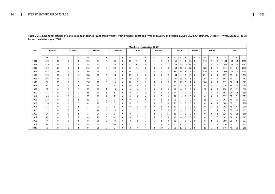
34 | ICES SCIENTIFIC REPORTS 3:26 | ICES
Table 2.2.1.3. Nominal catches of Baltic Salmon in tonnes round fresh weight, from offshore, coast and river by country and region in 2001–2020. O=offshore, C=coast, R=river. See ICES (2018) for catches before year 2001.
Year Estonia Finland Latvia Lithuania Sweden
O C O C O C R O C O C R O C R O C R O C R O C R O C R GT2001 433 10 0 4 135 64 0 39 0 66 71 0 1 4 0 165 9 6 33 0 310 2 7 1181 164 13 13582002 319 15 0 6 154 51 0 29 0 47 61 0 1 9 0 178 9 10 64 0 225 3 6 1018 153 16 11872003 439 15 0 3 115 33 0 29 0 33 14 0 0 3 0 154 22 3 20 0 188 3 3 977 94 6 10762004 355 15 0 3 169 74 0 35 0 19 13 2 0 2 0 83 0 5 14 0 410 5 3 1085 112 11 12082005 199 15 0 1 188 58 0 24 0 15 8 0 0 2 0 104 5 5 12 0 291 5 2 833 95 8 9362006 163 15 0 1 105 22 0 18 0 9 5 0 0 2 0 100 12 6 3 0 198 3 1 594 60 7 6612007 64 15 0 2 158 11 0 15 0 16 3 7 0 2 0 75 15 5 4 0 188 4 2 519 52 14 5852008 19 15 0 2 46 16 0 21 0 0 5 4 0 2 0 30 8 6 4 0 60 6 2 179 55 11 2442009 82 0 0 2 39 16 1 14 0 0 10 5 0 1 1 42 8 0 0 0 82 8 1 258 45 7 3102010 145 0 0 1 36 11 1 8 0 0 4 10 0 1 1 40 7 0 0 0 128 5 1 357 28 12 3982011 105 0 0 1 38 18 1 7 0 0 4 4 0 0 1 22 9 0 0 0 162 5 1 335 37 7 3792012 118 0 0 2 23 27 0 7 0 0 2 6 0 1 1 25 3 0 0 0 88 6 2 261 40 10 3122013 138 0 0 2 0 21 0 6 0 0 6 5 0 0 1 21 3 0 0 0 0 5 1 166 37 7 2102014 143 0 0 2 1 29 0 6 0 0 5 5 0 1 1 13 3 0 0 0 0 6 1 163 46 8 2162015 112 0 0 3 2 24 0 10 0 1 6 3 3 0 9 15 3 0 0 0 0 1 2 143 37 15 1952016 94 0 0 3 1 24 0 8 0 0 7 1 8 0 11 15 3 0 0 0 0 3 1 126 41 13 1802017 46 0 0 3 0 21 0 42 0 0 5 3 5 0 3 49 6 0 0 0 0 2 0 143 36 6 1852018 74 0 0 3 0 26 0 49 0 2 1 3 6 1 4 59 7 0 0 0 0 2 0 190 39 8 2372019 98 0 0 3 0 32 0 49 0 12 4 4 7 1 2 45 20 0 0 0 0 1 1 210 60 7 2772020 78 0 0 3 0 21 0 9 0 8 4 4 0 10 6 38 10 0 0 0 16 1 1 149 49 11 208
Denmark Poland TotalMain Basin (subdivisions 22–29)
RussiaGermany
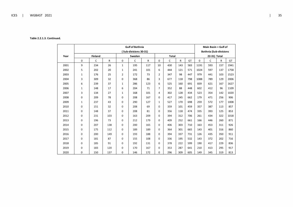
ICES | WGBAST 2021 | 35
Table 2.2.1.3. Continued.
Year Finland Sweden Total0 C R 0 C R 0 C R GT 0 C R GT
2001 9 234 26 1 195 117 10 430 143 583 1191 593 157 19412002 5 202 20 1 241 101 6 444 121 571 1024 597 137 17582003 1 176 25 2 172 73 2 347 98 447 979 441 103 15232004 3 309 32 0 368 86 3 677 118 798 1088 789 129 20062005 6 239 37 1 286 123 6 525 160 691 839 621 167 16272006 1 148 17 6 204 71 7 352 88 448 602 412 96 11092007 3 134 27 1 168 101 4 302 128 434 523 354 142 10202008 0 209 78 0 208 167 0 417 245 662 179 471 256 9062009 1 237 43 0 290 127 1 527 170 698 259 572 177 10082010 0 151 32 0 208 69 0 359 101 459 357 387 113 8572011 0 148 37 0 208 81 0 356 118 474 335 393 125 8532012 0 231 103 0 163 209 0 394 312 706 261 434 322 10182013 0 196 73 0 212 179 0 409 252 661 166 446 260 8712014 0 207 138 0 200 165 0 406 303 710 163 453 311 9262015 0 175 112 0 189 189 0 364 301 665 143 401 316 8602016 0 200 149 0 193 188 0 394 337 731 126 435 350 9112017 0 181 87 0 155 108 0 336 195 532 143 372 202 7162018 0 185 91 0 192 131 0 378 222 599 190 417 229 8362019 0 183 120 0 170 167 0 353 287 641 210 413 295 9172020 0 150 137 0 146 172 0 296 309 605 149 345 319 813
Gulf of Bothnia Main Basin + Gulf of ( Sub-divisions 30-31) Bothnia (Sub-divisions
22-31) Total
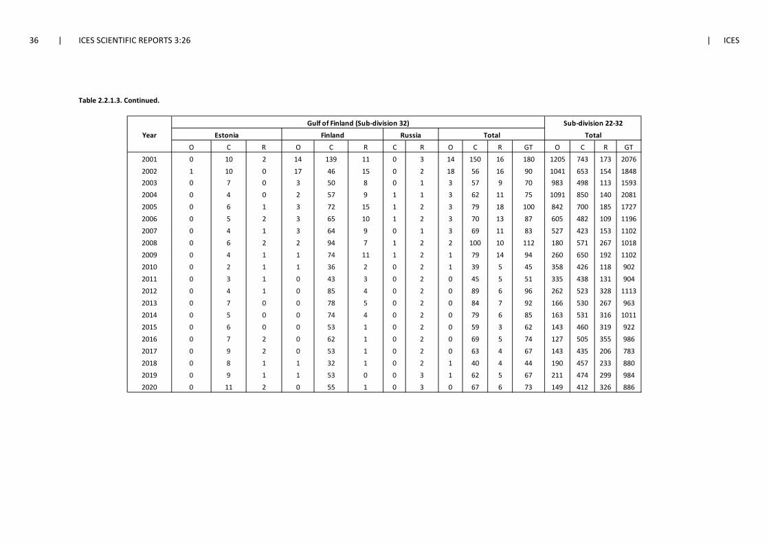
36 | ICES SCIENTIFIC REPORTS 3:26 | ICES
Table 2.2.1.3. Continued.
Gulf of Finland (Sub-division 32)Year Estonia Finland Russia Total
O C R O C R C R O C R GT O C R GT2001 0 10 2 14 139 11 0 3 14 150 16 180 1205 743 173 20762002 1 10 0 17 46 15 0 2 18 56 16 90 1041 653 154 18482003 0 7 0 3 50 8 0 1 3 57 9 70 983 498 113 15932004 0 4 0 2 57 9 1 1 3 62 11 75 1091 850 140 20812005 0 6 1 3 72 15 1 2 3 79 18 100 842 700 185 17272006 0 5 2 3 65 10 1 2 3 70 13 87 605 482 109 11962007 0 4 1 3 64 9 0 1 3 69 11 83 527 423 153 11022008 0 6 2 2 94 7 1 2 2 100 10 112 180 571 267 10182009 0 4 1 1 74 11 1 2 1 79 14 94 260 650 192 11022010 0 2 1 1 36 2 0 2 1 39 5 45 358 426 118 9022011 0 3 1 0 43 3 0 2 0 45 5 51 335 438 131 9042012 0 4 1 0 85 4 0 2 0 89 6 96 262 523 328 11132013 0 7 0 0 78 5 0 2 0 84 7 92 166 530 267 9632014 0 5 0 0 74 4 0 2 0 79 6 85 163 531 316 10112015 0 6 0 0 53 1 0 2 0 59 3 62 143 460 319 9222016 0 7 2 0 62 1 0 2 0 69 5 74 127 505 355 9862017 0 9 2 0 53 1 0 2 0 63 4 67 143 435 206 7832018 0 8 1 1 32 1 0 2 1 40 4 44 190 457 233 8802019 0 9 1 1 53 0 0 3 1 62 5 67 211 474 299 9842020 0 11 2 0 55 1 0 3 0 67 6 73 149 412 326 886
TotalSub-division 22-32
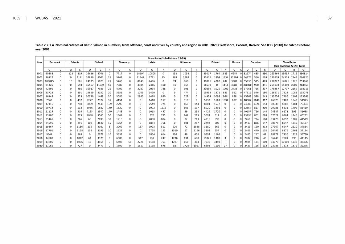
ICES | WGBAST 2021 | 37
Table 2.2.1.4. Nominal catches of Baltic Salmon in numbers, from offshore, coast and river by country and region in 2001–2020 O=offshore, C=coast, R=river. See ICES (2018) for catches before year 2001.
Main Basin (Sub-divisions 22-29)Year Estonia Latvia Poland Sweden
O C O C O C R O C O C R O C R O C R O C O C R O C R GT2001 90388 0 122 819 26616 8706 0 7717 0 18194 10808 0 152 1053 0 33017 1764 825 6584 0 82674 485 890 265464 23635 1715 2908142002 76122 0 0 1171 32870 8003 25 5762 0 11942 9781 85 363 2988 0 35636 1804 1934 12804 0 64275 556 699 239774 24303 2743 2668202003 108845 0 16 681 24975 5021 25 5766 0 8843 2496 0 74 966 0 30886 4282 632 3982 0 55335 575 469 238722 14021 1126 2538692004 81425 0 0 594 35567 11024 50 7087 0 4984 2316 400 49 655 0 16539 0 1111 4983 0 ###### 900 441 251078 15489 2002 2685692005 42491 0 0 286 36917 7936 25 4799 0 2787 2054 788 0 691 0 20869 1025 1002 2433 0 67961 715 337 178257 12707 2152 1931162006 33723 0 0 291 19859 3152 20 3551 0 1705 1490 0 9 474 0 19953 1371 883 552 0 47319 546 180 126671 7324 1083 1350782007 16145 0 0 325 30390 1468 20 3086 0 2960 1478 880 0 529 0 14924 3098 966 888 0 45263 598 243 113656 7496 2109 1232612008 7363 0 0 432 9277 2324 35 4151 0 0 1410 157 0 518 0 5933 1683 1034 697 0 18602 1040 317 46023 7407 1543 549732009 17116 0 0 740 8039 2435 109 2799 0 0 2549 774 0 166 144 8301 1572 0 0 0 24080 1326 154 60335 8788 1181 703042010 29714 0 0 538 6966 1587 140 1520 0 0 1092 1215 0 106 137 8029 1491 0 0 0 32857 817 210 79086 5631 1702 864192011 21125 0 0 414 7193 2340 140 1483 0 0 1013 457 0 59 258 4429 1720 0 0 0 40157 726 144 74387 6272 999 816582012 23180 0 0 713 4088 3560 50 1362 0 0 576 795 0 142 213 5094 511 0 0 0 23798 862 288 57522 6364 1346 652322013 25461 0 0 766 66 2699 30 1210 0 0 2038 804 0 72 213 4215 593 0 0 0 2468 724 160 33420 6892 1207 415192014 24596 0 0 891 108 3840 15 1264 0 0 1884 766 0 101 287 2494 505 0 0 0 2413 826 147 30875 8047 1215 401372015 19367 0 0 1186 235 3081 8 2009 0 137 1923 512 620 72 1888 3180 565 0 0 0 2419 120 212 27967 6947 2620 375342016 17701 0 0 1158 152 3196 10 1623 0 0 2728 153 1510 97 2196 3102 557 0 0 0 2409 440 102 26497 8176 2461 371342017 9644 0 0 863 0 2978 10 5632 0 0 1864 614 996 48 658 9594 1166 0 0 2405 217 41 28271 7136 1323 367302018 14588 0 0 1042 64 3375 0 6586 0 347 937 247 1236 131 600 11021 1300 3 0 0 2407 216 45 36249 7001 895 441452019 13805 0 0 1036 13 4155 0 6408 56 2226 1138 753 1287 166 384 7936 3498 0 0 2404 131 100 34079 10180 1237 454962020 11065 0 0 727 0 2473 0 1599 0 1517 1158 676 82 1729 1057 6393 1105 27 0 0 2429 126 112 23085 7318 1872 32275
(sub-divisions 22-29) TotalMain BasinDenmark Finland Lithuania RussiaGermany
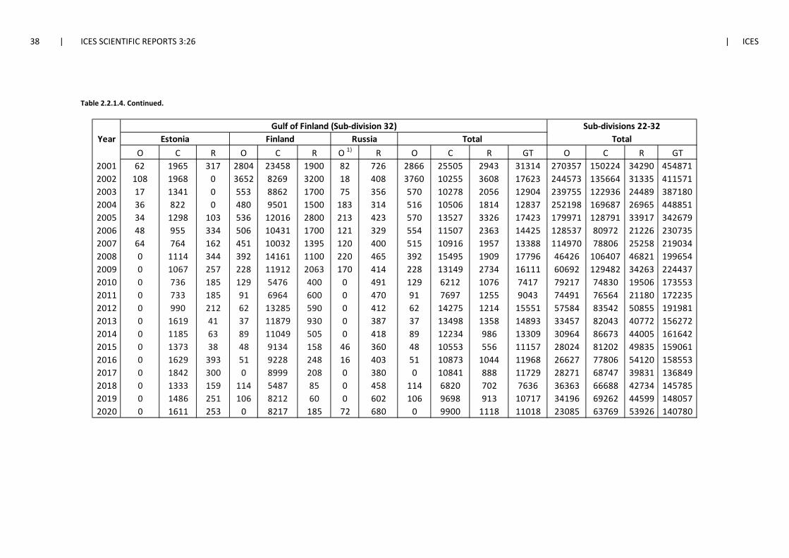
38 | ICES SCIENTIFIC REPORTS 3:26 | ICES
Table 2.2.1.4. Continued.
Gulf of Finland (Sub-division 32)Year Estonia Finland Russia Total
O C R O C R O 1) R O C R GT O C R GT2001 62 1965 317 2804 23458 1900 82 726 2866 25505 2943 31314 270357 150224 34290 4548712002 108 1968 0 3652 8269 3200 18 408 3760 10255 3608 17623 244573 135664 31335 4115712003 17 1341 0 553 8862 1700 75 356 570 10278 2056 12904 239755 122936 24489 3871802004 36 822 0 480 9501 1500 183 314 516 10506 1814 12837 252198 169687 26965 4488512005 34 1298 103 536 12016 2800 213 423 570 13527 3326 17423 179971 128791 33917 3426792006 48 955 334 506 10431 1700 121 329 554 11507 2363 14425 128537 80972 21226 2307352007 64 764 162 451 10032 1395 120 400 515 10916 1957 13388 114970 78806 25258 2190342008 0 1114 344 392 14161 1100 220 465 392 15495 1909 17796 46426 106407 46821 1996542009 0 1067 257 228 11912 2063 170 414 228 13149 2734 16111 60692 129482 34263 2244372010 0 736 185 129 5476 400 0 491 129 6212 1076 7417 79217 74830 19506 1735532011 0 733 185 91 6964 600 0 470 91 7697 1255 9043 74491 76564 21180 1722352012 0 990 212 62 13285 590 0 412 62 14275 1214 15551 57584 83542 50855 1919812013 0 1619 41 37 11879 930 0 387 37 13498 1358 14893 33457 82043 40772 1562722014 0 1185 63 89 11049 505 0 418 89 12234 986 13309 30964 86673 44005 1616422015 0 1373 38 48 9134 158 46 360 48 10553 556 11157 28024 81202 49835 1590612016 0 1629 393 51 9228 248 16 403 51 10873 1044 11968 26627 77806 54120 1585532017 0 1842 300 0 8999 208 0 380 0 10841 888 11729 28271 68747 39831 1368492018 0 1333 159 114 5487 85 0 458 114 6820 702 7636 36363 66688 42734 1457852019 0 1486 251 106 8212 60 0 602 106 9698 913 10717 34196 69262 44599 1480572020 0 1611 253 0 8217 185 72 680 0 9900 1118 11018 23085 63769 53926 140780
TotalSub-divisions 22-32
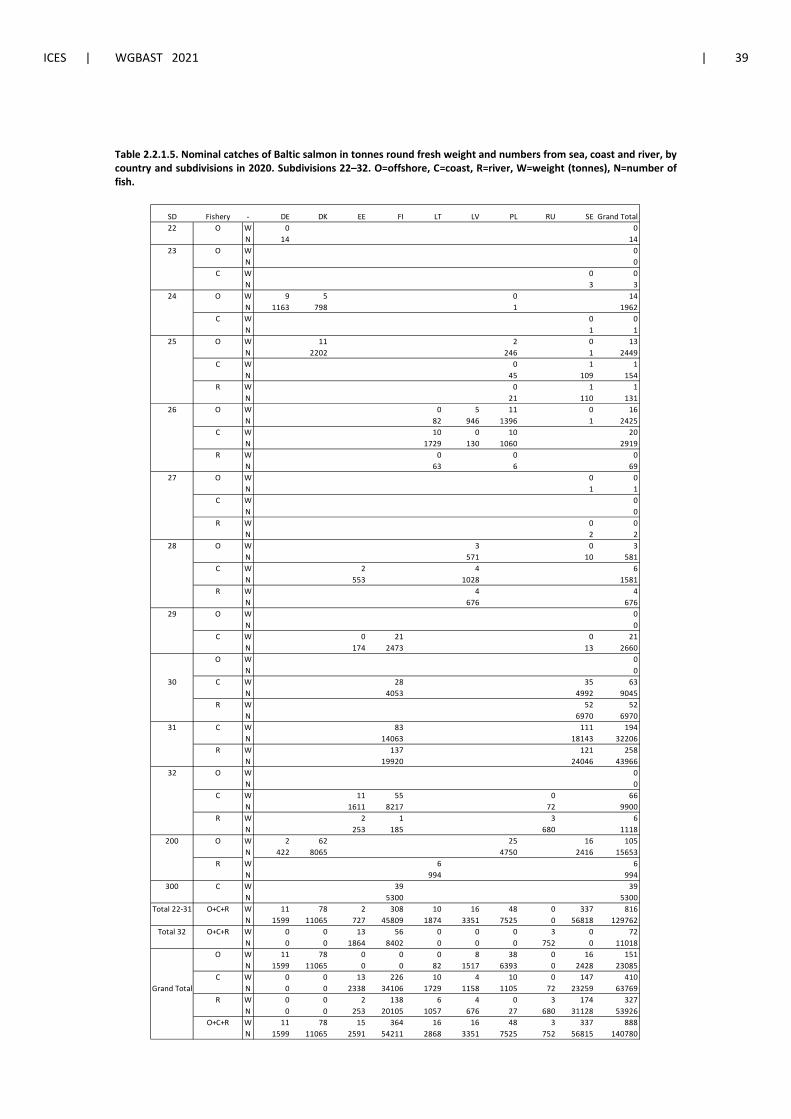
ICES | WGBAST 2021 | 39
Table 2.2.1.5. Nominal catches of Baltic salmon in tonnes round fresh weight and numbers from sea, coast and river, by country and subdivisions in 2020. Subdivisions 22–32. O=offshore, C=coast, R=river, W=weight (tonnes), N=number of fish.
SD Fishery - DE DK EE FI LT LV PL RU SE Grand TotalO W 0 0
N 14 1423 O W 0
N 0C W 0 0
N 3 324 O W 9 5 0 14
N 1163 798 1 1962C W 0 0
N 1 125 O W 11 2 0 13
N 2202 246 1 2449C W 0 1 1
N 45 109 154R W 0 1 1
N 21 110 13126 O W 0 5 11 0 16
N 82 946 1396 1 2425C W 10 0 10 20
N 1729 130 1060 2919R W 0 0 0
N 63 6 6927 O W 0 0
N 1 1C W 0
N 0R W 0 0
N 2 2O W 3 0 3
N 571 10 581C W 2 4 6
N 553 1028 1581R W 4 4
N 676 67629 O W 0
N 0C W 0 21 0 21
N 174 2473 13 2660O W 0
N 030 C W 28 35 63
N 4053 4992 9045R W 52 52
N 6970 697031 C W 83 111 194
N 14063 18143 32206R W 137 121 258
N 19920 24046 4396632 O W 0
N 0C W 11 55 0 66
N 1611 8217 72 9900R W 2 1 3 6
N 253 185 680 1118200 O W 2 62 25 16 105
N 422 8065 4750 2416 15653R W 6 6
N 994 994300 C W 39 39
N 5300 5300Total 22-31 O+C+R W 11 78 2 308 10 16 48 0 337 816
N 1599 11065 727 45809 1874 3351 7525 0 56818 129762Total 32 O+C+R W 0 0 13 56 0 0 0 3 0 72
N 0 0 1864 8402 0 0 0 752 0 11018O W 11 78 0 0 0 8 38 0 16 151
N 1599 11065 0 0 82 1517 6393 0 2428 23085C W 0 0 13 226 10 4 10 0 147 410
Grand Total N 0 0 2338 34106 1729 1158 1105 72 23259 63769R W 0 0 2 138 6 4 0 3 174 327
N 0 0 253 20105 1057 676 27 680 31128 53926O+C+R W 11 78 15 364 16 16 48 3 337 888
N 1599 11065 2591 54211 2868 3351 7525 752 56815 140780
22
28
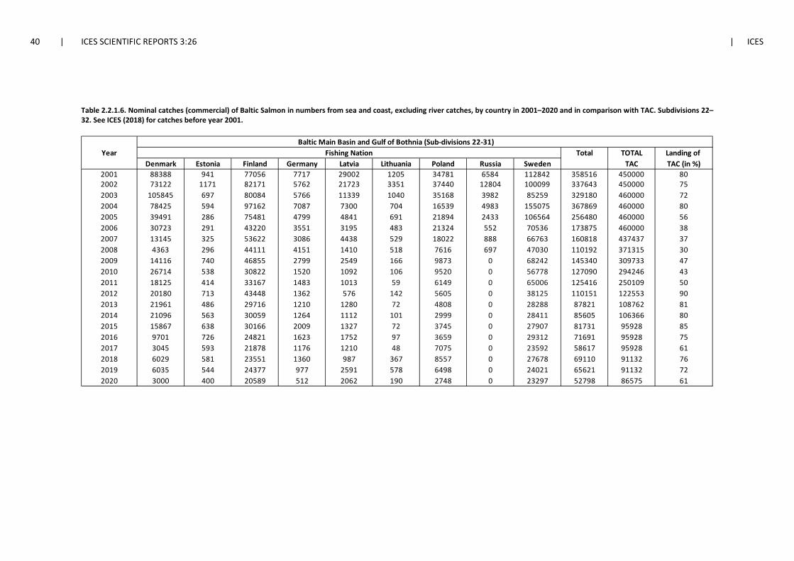
40 | ICES SCIENTIFIC REPORTS 3:26 | ICES
Table 2.2.1.6. Nominal catches (commercial) of Baltic Salmon in numbers from sea and coast, excluding river catches, by country in 2001–2020 and in comparison with TAC. Subdivisions 22–32. See ICES (2018) for catches before year 2001.
Year Total TOTAL Landing of Denmark Estonia Finland Germany Latvia Lithuania Poland Russia Sweden TAC TAC (in %)
2001 88388 941 77056 7717 29002 1205 34781 6584 112842 358516 450000 802002 73122 1171 82171 5762 21723 3351 37440 12804 100099 337643 450000 752003 105845 697 80084 5766 11339 1040 35168 3982 85259 329180 460000 722004 78425 594 97162 7087 7300 704 16539 4983 155075 367869 460000 802005 39491 286 75481 4799 4841 691 21894 2433 106564 256480 460000 562006 30723 291 43220 3551 3195 483 21324 552 70536 173875 460000 382007 13145 325 53622 3086 4438 529 18022 888 66763 160818 437437 372008 4363 296 44111 4151 1410 518 7616 697 47030 110192 371315 302009 14116 740 46855 2799 2549 166 9873 0 68242 145340 309733 472010 26714 538 30822 1520 1092 106 9520 0 56778 127090 294246 432011 18125 414 33167 1483 1013 59 6149 0 65006 125416 250109 502012 20180 713 43448 1362 576 142 5605 0 38125 110151 122553 902013 21961 486 29716 1210 1280 72 4808 0 28288 87821 108762 812014 21096 563 30059 1264 1112 101 2999 0 28411 85605 106366 802015 15867 638 30166 2009 1327 72 3745 0 27907 81731 95928 852016 9701 726 24821 1623 1752 97 3659 0 29312 71691 95928 752017 3045 593 21878 1176 1210 48 7075 0 23592 58617 95928 612018 6029 581 23551 1360 987 367 8557 0 27678 69110 91132 762019 6035 544 24377 977 2591 578 6498 0 24021 65621 91132 722020 3000 400 20589 512 2062 190 2748 0 23297 52798 86575 61
Baltic Main Basin and Gulf of Bothnia (Sub-divisions 22-31)Fishing Nation
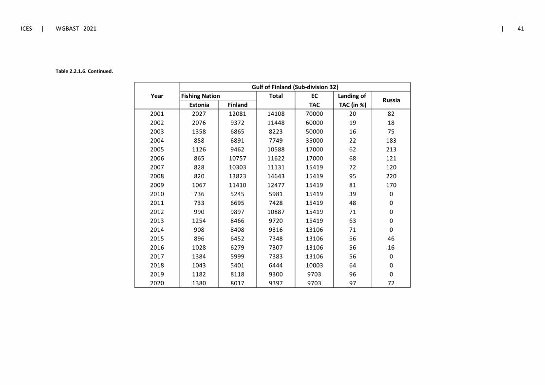
ICES | WGBAST 2021 | 41
Table 2.2.1.6. Continued.
Year Fishing Nation Total EC Landing of Estonia Finland TAC TAC (in %)
2001 2027 12081 14108 70000 20 822002 2076 9372 11448 60000 19 182003 1358 6865 8223 50000 16 752004 858 6891 7749 35000 22 1832005 1126 9462 10588 17000 62 2132006 865 10757 11622 17000 68 1212007 828 10303 11131 15419 72 1202008 820 13823 14643 15419 95 2202009 1067 11410 12477 15419 81 1702010 736 5245 5981 15419 39 02011 733 6695 7428 15419 48 02012 990 9897 10887 15419 71 02013 1254 8466 9720 15419 63 02014 908 8408 9316 13106 71 02015 896 6452 7348 13106 56 462016 1028 6279 7307 13106 56 162017 1384 5999 7383 13106 56 02018 1043 5401 6444 10003 64 02019 1182 8118 9300 9703 96 02020 1380 8017 9397 9703 97 72
Russia
Gulf of Finland (Sub-division 32)
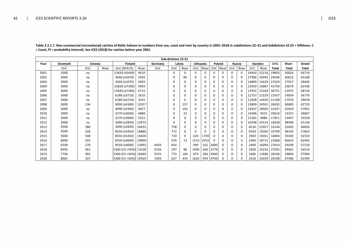
42 | ICES SCIENTIFIC REPORTS 3:26 | ICES
Table 2.2.1.7. Non-commercial (recreational) catches of Baltic Salmon in numbers from sea, coast and river by country in 2001–2018 in subdivisions 22–31 and Subdivision 32 (O = Offshore, C = Coast, PI = probability interval). See ICES (2018) for catches before year 2001.
Year O+C River GrandO+C River River O+C River O+C River O+C River O+C River O+C River Total Total Total
2001 na 4610 0 0 0 0 0 0 0 0 14443 22216 29893 26826 567192002 na 3592 0 85 0 0 0 0 0 0 17906 16945 24546 20622 451682003 na 4493 0 0 0 0 0 0 0 0 14889 13424 21529 17917 394462004 na 5992 0 0 0 0 0 0 0 0 22939 14687 41759 20679 624382005 na 6715 0 0 0 0 0 0 0 0 17931 15260 36751 21975 587262006 na 2610 0 0 0 0 0 0 0 0 12757 12229 21937 14839 367762007 na 3541 0 0 0 0 0 0 0 0 11928 14429 21108 17970 390782008 136 12027 0 157 0 0 0 0 0 0 13809 24501 26035 36685 627202009 na 6957 0 192 0 0 0 0 0 0 19347 18505 31437 25654 570912010 na 4884 0 22 0 0 0 0 0 0 14346 9325 20616 14231 348472011 na 5521 0 0 0 0 0 0 0 0 11581 9886 17851 15407 332582012 na 12975 0 0 0 0 0 0 0 0 10548 25523 16638 38498 551362013 280 10635 758 0 0 0 0 0 0 0 6516 22057 14144 32692 468362014 328 18880 772 0 0 0 0 0 0 0 6559 19265 19709 38145 578542015 548 14420 733 0 620 1749 0 0 0 0 2943 19261 16894 35430 523242016 432 19890 976 13 1510 2010 0 0 0 0 2400 18711 21868 40624 624922017 270 12893 654 996 562 3685 0 0 0 2400 16094 27610 29549 571592018 461 13528 297 98 1000 600 3776 0 0 0 2400 15235 27055 29461 565162019 492 16640 773 184 874 384 4940 0 0 0 2400 12686 28100 29894 579942020 327 19920 627 443 1620 994 4750 0 0 0 2416 16039 24198 37396 615948065 5300 (CV >50%) 1093
8595 5300 (CV >50%) 52267796 5300 (CV >50%) 5525
8000 8550 (±4000)6599 8550 (±4000) 4456
3500 8550 (±5450)3500 8550 (±5450)
3000 3090 (±2830)3500 3090 (±2830)
3000 3270 (±3600)3000 3270 (±3600)
3000 9090 (±4380)3000 9090 (±4380)
3000 6180 (±3710)3000 6180 (±3710)
3000 15820 (±7300)3000 15820 (±7300)
3000 3640 (±1070)3000 3640 (±1070)
O+C O+C (95% PI) O+C2000 13450 (±5490)
Sub-divisions 22-31Denmark Estonia Finland Germany Latvia Lithuania Poland Russia Sweden
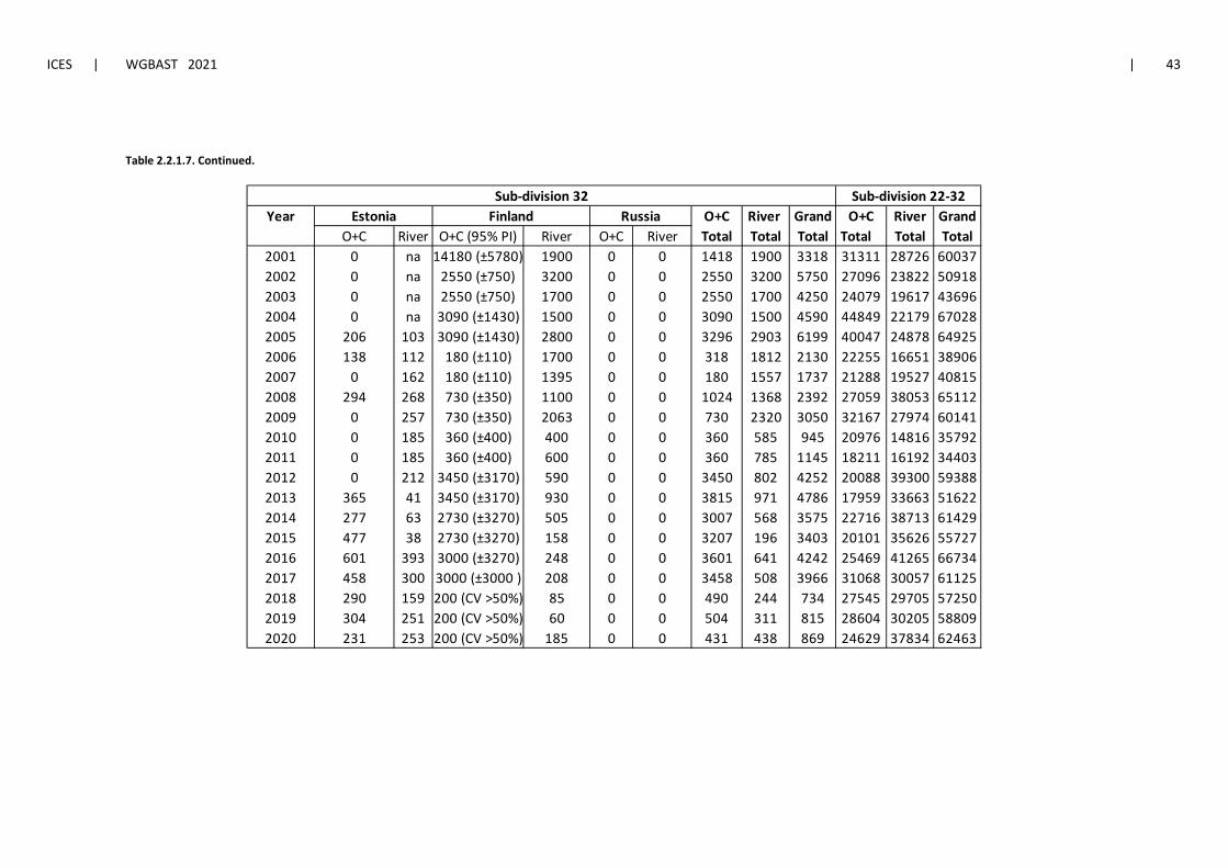
ICES | WGBAST 2021 | 43
Table 2.2.1.7. Continued.
Year O+C River Grand O+C River GrandO+C River O+C (95% PI) River O+C River Total Total Total Total Total Total
2001 0 na 14180 (±5780) 1900 0 0 1418 1900 3318 31311 28726 600372002 0 na 2550 (±750) 3200 0 0 2550 3200 5750 27096 23822 509182003 0 na 2550 (±750) 1700 0 0 2550 1700 4250 24079 19617 436962004 0 na 3090 (±1430) 1500 0 0 3090 1500 4590 44849 22179 670282005 206 103 3090 (±1430) 2800 0 0 3296 2903 6199 40047 24878 649252006 138 112 180 (±110) 1700 0 0 318 1812 2130 22255 16651 389062007 0 162 180 (±110) 1395 0 0 180 1557 1737 21288 19527 408152008 294 268 730 (±350) 1100 0 0 1024 1368 2392 27059 38053 651122009 0 257 730 (±350) 2063 0 0 730 2320 3050 32167 27974 601412010 0 185 360 (±400) 400 0 0 360 585 945 20976 14816 357922011 0 185 360 (±400) 600 0 0 360 785 1145 18211 16192 344032012 0 212 3450 (±3170) 590 0 0 3450 802 4252 20088 39300 593882013 365 41 3450 (±3170) 930 0 0 3815 971 4786 17959 33663 516222014 277 63 2730 (±3270) 505 0 0 3007 568 3575 22716 38713 614292015 477 38 2730 (±3270) 158 0 0 3207 196 3403 20101 35626 557272016 601 393 3000 (±3270) 248 0 0 3601 641 4242 25469 41265 667342017 458 300 3000 (±3000 ) 208 0 0 3458 508 3966 31068 30057 611252018 290 159 200 (CV >50%) 85 0 0 490 244 734 27545 29705 572502019 304 251 200 (CV >50%) 60 0 0 504 311 815 28604 30205 588092020 231 253 200 (CV >50%) 185 0 0 431 438 869 24629 37834 62463
Estonia Finland RussiaSub-division 32 Sub-division 22-32
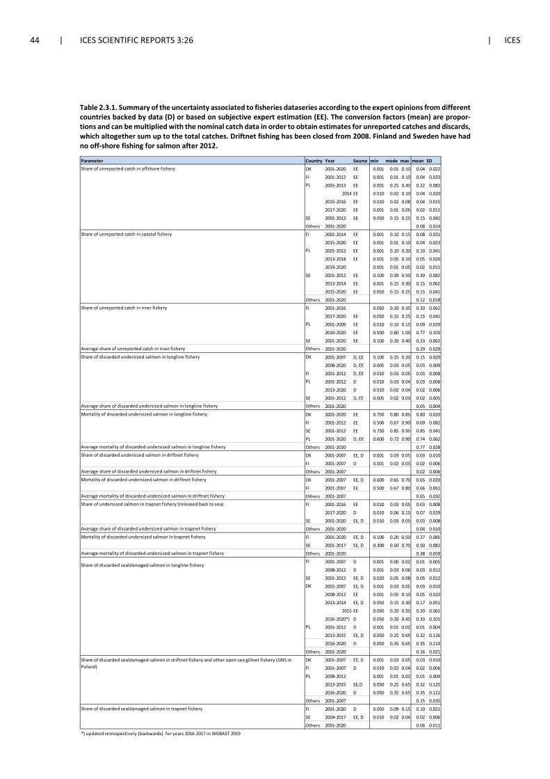
44 | ICES SCIENTIFIC REPORTS 3:26 | ICES
Table 2.3.1. Summary of the uncertainty associated to fisheries dataseries according to the expert opinions from different countries backed by data (D) or based on subjective expert estimation (EE). The conversion factors (mean) are propor-tions and can be multiplied with the nominal catch data in order to obtain estimates for unreported catches and discards, which altogether sum up to the total catches. Driftnet fishing has been closed from 2008. Finland and Sweden have had no off-shore fishing for salmon after 2012.
Parameter Country Year Source min mode max mean SDShare of unreported catch in offshore fishery DK 2001-2020 EE 0.001 0.01 0.10 0.04 0.022
FI 2001-2012 EE 0.001 0.01 0.10 0.04 0.023PL 2001-2013 EE 0.001 0.25 0.40 0.22 0.082
2014 EE 0.010 0.02 0.10 0.04 0.020
2015-2016 EE 0.010 0.02 0.08 0.04 0.015
2017-2020 EE 0.001 0.01 0.05 0.02 0.011
SE 2001-2012 EE 0.050 0.15 0.25 0.15 0.041
Others 2001-2020 0.08 0.014Share of unreported catch in coastal fishery FI 2001-2014 EE 0.001 0.10 0.15 0.08 0.031
2015-2020 EE 0.001 0.01 0.10 0.04 0.023PL 2001-2012 EE 0.001 0.10 0.20 0.10 0.041
2013-2018 EE 0.001 0.05 0.10 0.05 0.020
2019-2020 0.001 0.01 0.05 0.02 0.011
SE 2001-2012 EE 0.100 0.30 0.50 0.30 0.082
2013-2014 EE 0.001 0.15 0.30 0.15 0.062
2015-2020 EE 0.050 0.15 0.25 0.15 0.041
Others 2001-2020 0.12 0.018Share of unreported catch in river fishery FI 2001-2016 0.050 0.20 0.35 0.20 0.062
2017-2020 EE 0.050 0.15 0.25 0.15 0.041PL 2001-2009 EE 0.010 0.10 0.15 0.09 0.029
2010-2020 EE 0.500 0.80 1.00 0.77 0.103
SE 2001-2020 EE 0.100 0.20 0.40 0.23 0.062Average share of unreported catch in river fishery Others 2001-2020 0.29 0.029Share of discarded undersized salmon in longline fishery DK 2001-2007 D, EE 0.100 0.15 0.20 0.15 0.020
2008-2020 D, EE 0.005 0.03 0.05 0.03 0.009
FI 2001-2012 D, EE 0.010 0.03 0.05 0.03 0.008PL 2001-2012 D 0.010 0.03 0.04 0.03 0.006
2013-2020 D 0.010 0.02 0.04 0.02 0.006
SE 2001-2012 D, EE 0.005 0.02 0.03 0.02 0.005Average share of discarded undersized salmon in longline fishery Others 2001-2020 0.05 0.004Mortality of discarded undersized salmon in longline fishery DK 2001-2020 EE 0.750 0.80 0.85 0.80 0.020
FI 2001-2012 EE 0.500 0.67 0.90 0.69 0.082
SE 2001-2012 EE 0.750 0.85 0.95 0.85 0.041
PL 2001-2020 D, EE 0.600 0.72 0.90 0.74 0.062Average mortality of discarded undersized salmon in longline fishery Others 2001-2020 0.77 0.028Share of discarded undersized salmon in driftnet fishery DK 2001-2007 EE, D 0.001 0.03 0.05 0.03 0.010
FI 2001-2007 D 0.001 0.02 0.03 0.02 0.006Average share of discarded undersized salmon in driftnet fishery Others 2001-2007 0.02 0.006Mortality of discarded undersized salmon in driftnet fishery DK 2001-2007 EE, D 0.600 0.65 0.70 0.65 0.020
FI 2001-2007 EE 0.500 0.67 0.80 0.66 0.061Average mortality of discarded undersized salmon in driftnet fishery Others 2001-2007 0.65 0.032Share of undersized salmon in trapnet fishery (released back to sea) FI 2001-2016 EE 0.010 0.03 0.05 0.03 0.008
2017-2020 D 0.010 0.06 0.15 0.07 0.029
SE 2001-2020 EE, D 0.010 0.03 0.05 0.03 0.008Average share of discarded undersized salmon in trapnet fishery Others 2001-2020 0.04 0.010Mortality of discarded undersized salmon in trapnet fishery FI 2001-2020 EE, D 0.100 0.20 0.50 0.27 0.085
SE 2001-2017 EE, D 0.300 0.50 0.70 0.50 0.082Average mortality of discarded undersized salmon in trapnet fishery Others 2001-2020 0.38 0.059
FI 2001-2007 D 0.001 0.00 0.02 0.01 0.005
2008-2012 D 0.001 0.03 0.06 0.03 0.012
SE 2001-2012 EE, D 0.020 0.05 0.08 0.05 0.012DK 2001-2007 EE, D 0.001 0.03 0.05 0.03 0.010
2008-2012 EE 0.001 0.05 0.10 0.05 0.020
2013-2014 EE, D 0.050 0.15 0.30 0.17 0.051
2015 EE 0.050 0.20 0.35 0.20 0.061
2016-2020*) D 0.050 0.20 0.45 0.33 0.101PL 2001-2012 D 0.001 0.01 0.02 0.01 0.004
2013-2015 EE, D 0.050 0.25 0.65 0.32 0.126
2016-2020 D 0.050 0.35 0.65 0.35 0.124
Others 2001-2020 0.16 0.021
DK 2001-2007 EE, D 0.001 0.03 0.05 0.03 0.010
FI 2001-2007 D 0.010 0.02 0.04 0.02 0.006
PL 2008-2012 0.001 0.01 0.02 0.01 0.004
2013-2015 EE,D 0.050 0.25 0.65 0.32 0.125
2016-2020 D 0.050 0.35 0.65 0.35 0.122
Others 2001-2007 0.15 0.035Share of discarded sealdamaged salmon in trapnet fishery FI 2001-2020 D 0.050 0.09 0.15 0.10 0.021
SE 2004-2017 EE, D 0.010 0.02 0.04 0.02 0.006
Others 2001-2020 0.06 0.011
*) updated retrospectively (backwards) for years 2016-2017 in WGBAST 2019
Share of discarded sealdamaged salmon in longline fishery
Share of discarded sealdamaged salmon in driftnet fishery and other open sea gillnet fishery (GNS in Poland)
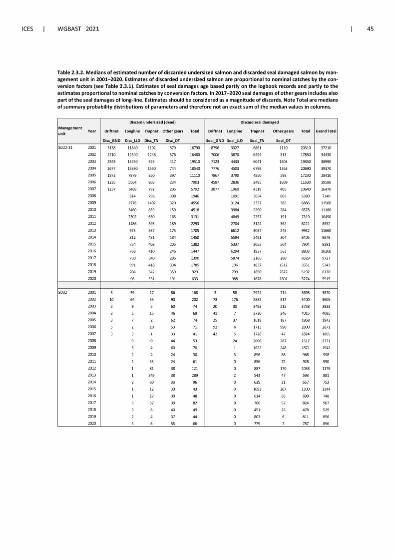
ICES | WGBAST 2021 | 45
Table 2.3.2. Medians of estimated number of discarded undersized salmon and discarded seal damaged salmon by man-agement unit in 2001–2020. Estimates of discarded undersized salmon are proportional to nominal catches by the con-version factors (see Table 2.3.1). Estimates of seal damages age based partly on the logbook records and partly to the estimates proportional to nominal catches by conversion factors. In 2017–2020 seal damages of other gears includes also part of the seal damages of long-line. Estimates should be considered as a magnitude of discards. Note Total are medians of summary probability distributions of parameters and therefore not an exact sum of the median values in columns.
Management unit Year Driftnet Longline Trapnet Other gears Total Driftnet Longline Trapnet Other gears Total Grand Total
Disc_GND Disc_LLD Disc_TN Disc_OT Seal_GND Seal_LLD Seal_TN Seal_OT
SD22-31 2001 3138 11840 1102 579 16790 8796 3327 6861 1110 20310 372102002 2210 12340 1248 576 16480 7006 3870 6494 313 17850 344302003 2343 15730 923 417 19510 7123 4433 6041 1603 19350 389902004 2677 13390 1560 744 18540 7776 4503 6799 1363 20690 393702005 1872 7879 850 397 11110 7867 3790 4850 598 17230 284102006 1235 5564 803 234 7903 4587 2836 2495 1609 11630 195802007 1237 3488 792 205 5792 3877 1960 4319 405 10640 164702008 814 796 308 1946 1091 3654 603 5380 73402009 2776 1402 320 4556 3124 3337 385 6886 115002010 3460 859 159 4518 3984 2290 284 6578 111802011 2302 630 165 3131 4849 2257 191 7319 104902012 1486 593 189 2293 2704 3124 362 6221 85522013 973 537 175 1705 6612 3057 245 9932 116602014 812 431 184 1450 5594 2491 304 8405 98792015 754 402 205 1382 5337 2053 504 7904 92912016 768 410 246 1447 6294 1937 563 8803 102602017 730 340 286 1390 5874 2166 280 8329 97272018 991 418 334 1785 196 1837 1512 3551 53432019 204 342 359 929 709 1850 2627 5192 61302020 96 331 191 633 988 1678 2601 5274 5915
SD32 2001 3 59 17 86 168 3 58 2924 714 3698 38702002 10 64 35 90 202 73 176 2832 317 3400 36052003 2 9 2 60 74 20 30 3493 215 3758 38332004 3 5 15 46 69 41 7 3720 246 4015 40852005 3 7 2 62 74 25 37 1618 187 1868 19432006 5 2 10 53 71 92 4 1713 990 2800 28712007 3 3 1 33 41 42 5 1728 47 1824 18652008 9 0 44 53 24 2006 287 2317 23712009 5 4 60 70 1 1622 248 1871 19422010 2 4 24 30 3 896 68 968 9982011 2 35 24 61 0 856 72 928 9902012 1 81 38 121 0 887 170 1058 11792013 1 249 38 289 2 543 47 593 8812014 2 60 33 96 0 635 21 657 7532015 1 12 30 43 0 1093 207 1300 13442016 1 17 30 48 0 614 85 699 7482017 5 37 39 82 0 766 57 824 9072018 3 6 40 49 0 451 26 478 5292019 2 4 37 44 0 803 6 811 8562020 5 6 55 66 0 779 7 787 856
Discard undersized (dead) Discard seal damaged
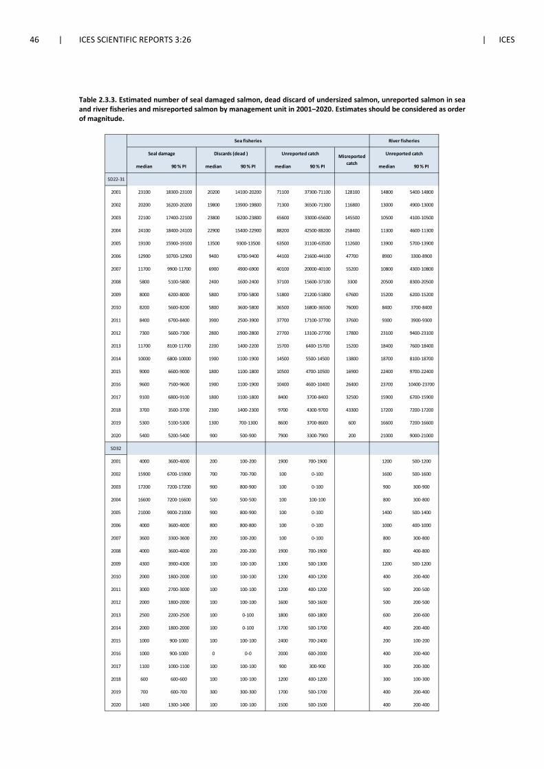
46 | ICES SCIENTIFIC REPORTS 3:26 | ICES
Table 2.3.3. Estimated number of seal damaged salmon, dead discard of undersized salmon, unreported salmon in sea and river fisheries and misreported salmon by management unit in 2001–2020. Estimates should be considered as order of magnitude.
median 90 % PI median 90 % PI median 90 % PI median 90 % PI
SD22-31
2001 23100 18300-23100 20200 14100-20200 71100 37300-71100 128100 14800 5400-14800
2002 20200 16200-20200 19800 13900-19800 71300 36500-71300 116800 13000 4900-13000
2003 22100 17400-22100 23800 16200-23800 65600 33000-65600 145500 10500 4100-10500
2004 24100 18400-24100 22900 15400-22900 88200 42500-88200 258400 11300 4600-11300
2005 19100 15900-19100 13500 9300-13500 63500 31100-63500 112600 13900 5700-13900
2006 12900 10700-12900 9400 6700-9400 44100 21600-44100 47700 8900 3300-8900
2007 11700 9900-11700 6900 4900-6900 40100 20000-40100 55200 10800 4300-10800
2008 5800 5100-5800 2400 1600-2400 37100 15600-37100 3300 20500 8300-20500
2009 8000 6200-8000 5800 3700-5800 51800 21200-51800 67600 15200 6200-15200
2010 8200 5600-8200 5800 3600-5800 36500 16800-36500 76000 8400 3700-8400
2011 8400 6700-8400 3900 2500-3900 37700 17100-37700 37600 9300 3900-9300
2012 7300 5600-7300 2800 1900-2800 27700 13100-27700 17800 23100 9400-23100
2013 11700 8100-11700 2200 1400-2200 15700 6400-15700 15200 18400 7600-18400
2014 10000 6800-10000 1900 1100-1900 14500 5500-14500 13800 18700 8100-18700
2015 9000 6600-9000 1800 1100-1800 10500 4700-10500 16900 22400 9700-22400
2016 9600 7500-9600 1900 1100-1900 10400 4600-10400 26400 23700 10400-23700
2017 9100 6800-9100 1800 1100-1800 8400 3700-8400 32500 15900 6700-15900
2018 3700 3500-3700 2300 1400-2300 9700 4300-9700 43300 17200 7200-17200
2019 5300 5100-5300 1300 700-1300 8600 3700-8600 600 16600 7200-16600
2020 5400 5200-5400 900 500-900 7900 3300-7900 200 21000 9000-21000
SD32
2001 4000 3600-4000 200 100-200 1900 700-1900 1200 500-1200
2002 15900 6700-15900 700 700-700 100 0-100 1600 500-1600
2003 17200 7200-17200 900 800-900 100 0-100 900 300-900
2004 16600 7200-16600 500 500-500 100 100-100 800 300-800
2005 21000 9000-21000 900 800-900 100 0-100 1400 500-1400
2006 4000 3600-4000 800 800-800 100 0-100 1000 400-1000
2007 3600 3300-3600 200 100-200 100 0-100 800 300-800
2008 4000 3600-4000 200 200-200 1900 700-1900 800 400-800
2009 4300 3900-4300 100 100-100 1300 500-1300 1200 500-1200
2010 2000 1800-2000 100 100-100 1200 400-1200 400 200-400
2011 3000 2700-3000 100 100-100 1200 400-1200 500 200-500
2012 2000 1800-2000 100 100-100 1600 500-1600 500 200-500
2013 2500 2200-2500 100 0-100 1800 600-1800 600 200-600
2014 2000 1800-2000 100 0-100 1700 500-1700 400 200-400
2015 1000 900-1000 100 100-100 2400 700-2400 200 100-200
2016 1000 900-1000 0 0-0 2000 600-2000 400 200-400
2017 1100 1000-1100 100 100-100 900 300-900 300 200-300
2018 600 600-600 100 100-100 1200 400-1200 300 100-300
2019 700 600-700 300 300-300 1700 500-1700 400 200-400
2020 1400 1300-1400 100 100-100 1500 500-1500 400 200-400
River fisheries
Seal damage Discards (dead ) Unreported catch Misreported catch
Unreported catch
Sea fisheries
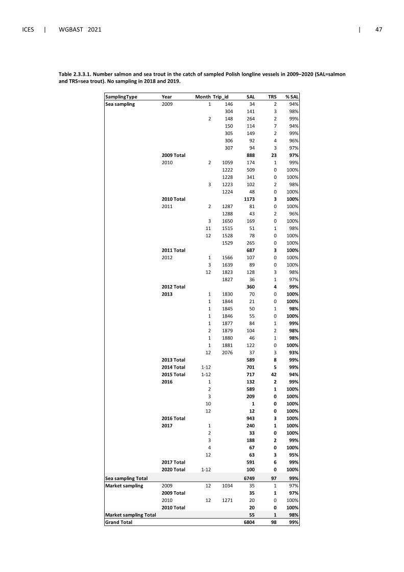
ICES | WGBAST 2021 | 47
Table 2.3.3.1. Number salmon and sea trout in the catch of sampled Polish longline vessels in 2009–2020 (SAL=salmon and TRS=sea trout). No sampling in 2018 and 2019.
SamplingType Year Month Trip_id SAL TRS % SALSea sampling 2009 1 146 34 2 94%
304 141 3 98%2 148 264 2 99%
150 114 7 94%305 149 2 99%306 92 4 96%307 94 3 97%
2009 Total 888 23 97%2010 2 1059 174 1 99%
1222 509 0 100%1228 341 0 100%
3 1223 102 2 98%1224 48 0 100%
2010 Total 1173 3 100%2011 2 1287 81 0 100%
1288 43 2 96%3 1650 169 0 100%
11 1515 51 1 98%12 1528 78 0 100%
1529 265 0 100%2011 Total 687 3 100%2012 1 1566 107 0 100%
3 1639 89 0 100%12 1823 128 3 98%
1827 36 1 97%2012 Total 360 4 99%2013 1 1830 70 0 100%
1 1844 21 0 100%1 1845 50 1 98%1 1846 55 0 100%1 1877 84 1 99%2 1879 104 2 98%1 1880 46 1 98%1 1881 122 0 100%
12 2076 37 3 93%2013 Total 589 8 99%2014 Total 1-12 701 5 99%2015 Total 1-12 717 42 94%2016 1 132 2 99%
2 589 1 100%3 209 0 100%
10 1 0 100%12 12 0 100%
2016 Total 943 3 100%2017 1 240 1 100%
2 33 0 100%3 188 2 99%4 67 0 100%
12 63 3 95%2017 Total 591 6 99%2020 Total 1-12 100 0 100%
Sea sampling Total 6749 97 99%Market sampling 2009 12 1034 35 1 97%
2009 Total 35 1 97%2010 12 1271 20 0 100%2010 Total 20 0 100%
Market sampling Total 55 1 98%Grand Total 6804 98 99%
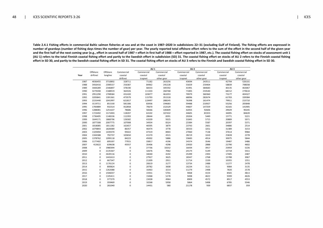
48 | ICES SCIENTIFIC REPORTS 3:26 | ICES
Table 2.4.1 Fishing efforts in commercial Baltic salmon fisheries at sea and at the coast in 1987–2020 in subdivisions 22–31 (excluding Gulf of Finland). The fishing efforts are expressed in number of geardays (number of fishing days times the number of gear) per year. The yearly reported total offshore effort refers to the sum of the effort in the second half of the given year and the first half of the next coming year (e.g., effort in second half of 1987 + effort in first half of 1988 = effort reported in 1987, etc.). The coastal fishing effort on stocks of assessment unit 1 (AU 1) refers to the total Finnish coastal fishing effort and partly to the Swedish effort in subdivision (SD) 31. The coastal fishing effort on stocks of AU 2 refers to the Finnish coastal fishing effort in SD 30, and partly to the Swedish coastal fishing effort in SD 31. The coastal fishing effort on stocks of AU 3 refers to the Finnish and Swedish coastal fishing effort in SD 30.
Offshore Offshore Commercial Commercial Commercial Commercial Commercial Commercial Commercial Year driftnet longline coastal coastal coastal coastal coastal coastal coastal
driftnet trapnet other gear trapnet other gear trapnet other gear1987 4036455 3710892 328711 71182 263256 43694 243511 42704 5261011988 3456416 2390537 256387 84962 245228 55659 259404 58839 7980381989 3444289 2346897 378190 68333 345592 41991 384683 40135 4630671990 3279200 2188919 364326 111333 260768 71005 233540 68152 2796101991 2951290 1708584 431420 103077 461053 70979 360360 73177 4043271992 3205841 1391361 473579 115793 351518 68096 282674 61703 3393841993 2155440 1041997 621817 119497 288245 76398 161474 79911 2157101994 3119711 851530 581306 83936 194683 59488 210927 55256 2058481995 1783889 932314 452858 70670 152529 44607 147259 42165 1419051996 1288081 1251637 78686 58266 100409 42055 92606 29029 902451997 1723492 1571003 118207 63102 107432 44605 81923 34095 846391998 1736495 1148336 112393 28644 8391 20204 5449 15771 52211999 1644171 1868796 126582 43339 9325 31845 5715 20889 50712000 1877308 2007775 107008 34934 8324 23384 5587 20397 53712001 1818085 1811282 102657 40595 3879 23743 2661 34886 25142002 1079893 1828389 86357 46474 3778 30333 3251 31389 31532003 1329494 1439370 95022 47319 8903 27060 7138 37614 99842004 1344588 792737 103650 41570 4315 28219 1610 25828 22782005 1378762 1099118 84223 45002 5886 33683 4914 30075 58442006 1177402 695597 77915 33817 4196 24374 3546 19487 54862007 413622 639638 45557 35406 4298 23920 2888 21790 46022008 0 1980394 0 27736 10252 16434 3917 25959 52262009 0 2135367 0 32676 7062 24174 5149 15718 54112010 0 2639116 0 34040 4192 25399 2393 17405 24872011 0 1441613 0 27927 3625 18347 2768 15788 30672012 0 667347 0 21309 2911 11714 1539 10355 15512013 0 1176124 0 20619 3177 13734 2488 11277 24782014 0 800824 0 20782 3608 16234 3121 9084 31352015 0 1262088 0 16463 3214 11279 2498 7820 25782016 0 1506037 0 15931 5701 9068 4154 8565 48132017 0 1105411 0 15068 5278 9498 4622 9399 46262018 0 377379 0 15028 4964 8909 4572 8917 45532019 0 359469 0 10268 5958 5864 5498 6785 55462020 0 281040 0 14431 580 21178 939 6837 359
AU 1 AU 2 AU 3
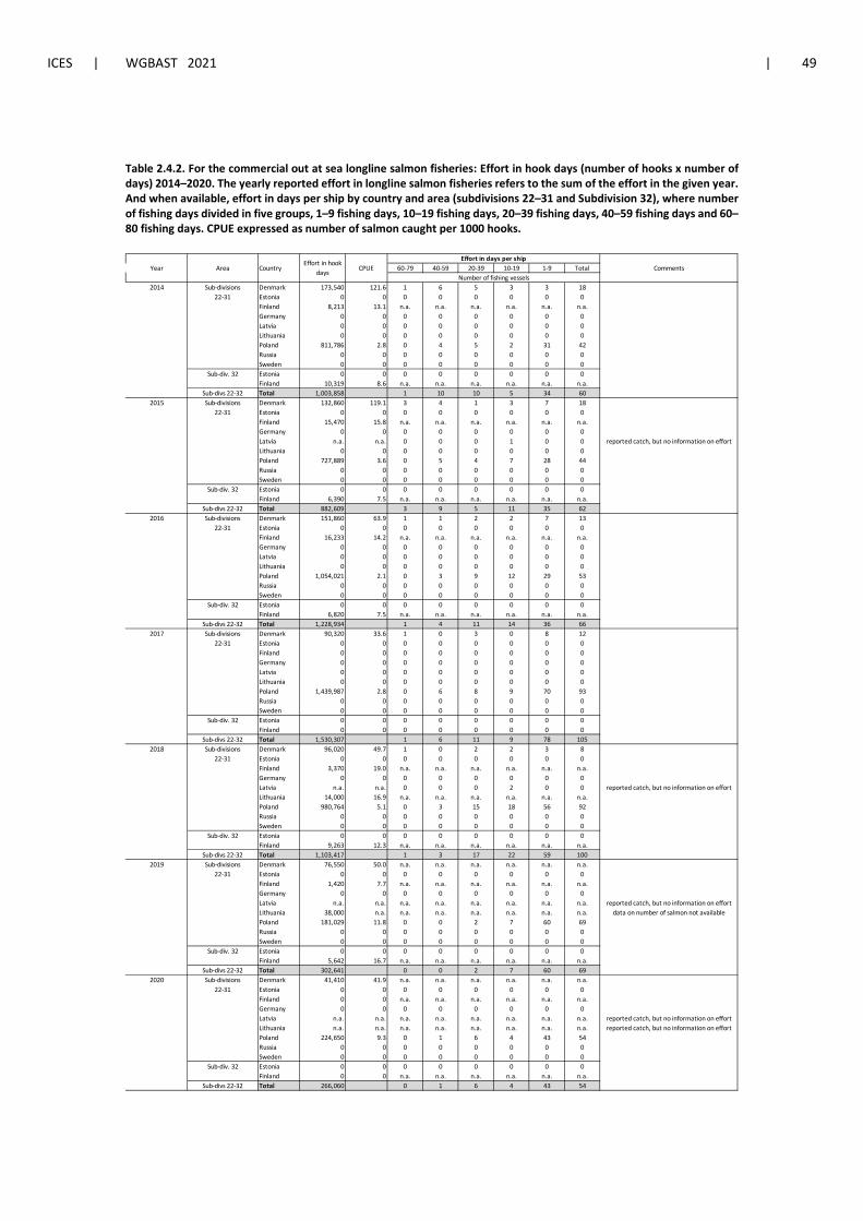
ICES | WGBAST 2021 | 49
Table 2.4.2. For the commercial out at sea longline salmon fisheries: Effort in hook days (number of hooks x number of days) 2014–2020. The yearly reported effort in longline salmon fisheries refers to the sum of the effort in the given year. And when available, effort in days per ship by country and area (subdivisions 22–31 and Subdivision 32), where number of fishing days divided in five groups, 1–9 fishing days, 10–19 fishing days, 20–39 fishing days, 40–59 fishing days and 60–80 fishing days. CPUE expressed as number of salmon caught per 1000 hooks.
Year Area Country CPUE 60-79 40-59 20-39 10-19 1-9 Total Comments
2014 Sub-divisions Denmark 173,540 121.6 1 6 5 3 3 1822-31 Estonia 0 0 0 0 0 0 0 0
Finland 8,213 13.1 n.a. n.a. n.a. n.a. n.a. n.a.Germany 0 0 0 0 0 0 0 0Latvia 0 0 0 0 0 0 0 0Lithuania 0 0 0 0 0 0 0 0Poland 811,786 2.8 0 4 5 2 31 42Russia 0 0 0 0 0 0 0 0Sweden 0 0 0 0 0 0 0 0
Sub-div. 32 Estonia 0 0 0 0 0 0 0 0Finland 10,319 8.6 n.a. n.a. n.a. n.a. n.a. n.a.
Sub-divs 22-32 Total 1,003,858 1 10 10 5 34 602015 Sub-divisions Denmark 132,860 119.1 3 4 1 3 7 18
22-31 Estonia 0 0 0 0 0 0 0 0Finland 15,470 15.8 n.a. n.a. n.a. n.a. n.a. n.a.Germany 0 0 0 0 0 0 0 0Latvia n.a. n.a. 0 0 0 1 0 0 reported catch, but no information on effortLithuania 0 0 0 0 0 0 0 0Poland 727,889 3.6 0 5 4 7 28 44Russia 0 0 0 0 0 0 0 0Sweden 0 0 0 0 0 0 0 0
Sub-div. 32 Estonia 0 0 0 0 0 0 0 0Finland 6,390 7.5 n.a. n.a. n.a. n.a. n.a. n.a.
Sub-divs 22-32 Total 882,609 3 9 5 11 35 622016 Sub-divisions Denmark 151,860 63.9 1 1 2 2 7 13
22-31 Estonia 0 0 0 0 0 0 0 0Finland 16,233 14.2 n.a. n.a. n.a. n.a. n.a. n.a.Germany 0 0 0 0 0 0 0 0Latvia 0 0 0 0 0 0 0 0Lithuania 0 0 0 0 0 0 0 0Poland 1,054,021 2.1 0 3 9 12 29 53Russia 0 0 0 0 0 0 0 0Sweden 0 0 0 0 0 0 0 0
Sub-div. 32 Estonia 0 0 0 0 0 0 0 0Finland 6,820 7.5 n.a. n.a. n.a. n.a. n.a. n.a.
Sub-divs 22-32 Total 1,228,934 1 4 11 14 36 662017 Sub-divisions Denmark 90,320 33.6 1 0 3 0 8 12
22-31 Estonia 0 0 0 0 0 0 0 0Finland 0 0 0 0 0 0 0 0Germany 0 0 0 0 0 0 0 0Latvia 0 0 0 0 0 0 0 0Lithuania 0 0 0 0 0 0 0 0Poland 1,439,987 2.8 0 6 8 9 70 93Russia 0 0 0 0 0 0 0 0Sweden 0 0 0 0 0 0 0 0
Sub-div. 32 Estonia 0 0 0 0 0 0 0 0Finland 0 0 0 0 0 0 0 0
Sub-divs 22-32 Total 1,530,307 1 6 11 9 78 1052018 Sub-divisions Denmark 96,020 49.7 1 0 2 2 3 8
22-31 Estonia 0 0 0 0 0 0 0 0Finland 3,370 19.0 n.a. n.a. n.a. n.a. n.a. n.a.Germany 0 0 0 0 0 0 0 0Latvia n.a. n.a. 0 0 0 2 0 0 reported catch, but no information on effortLithuania 14,000 16.9 n.a. n.a. n.a. n.a. n.a. n.a.Poland 980,764 5.1 0 3 15 18 56 92Russia 0 0 0 0 0 0 0 0Sweden 0 0 0 0 0 0 0 0
Sub-div. 32 Estonia 0 0 0 0 0 0 0 0Finland 9,263 12.3 n.a. n.a. n.a. n.a. n.a. n.a.
Sub-divs 22-32 Total 1,103,417 1 3 17 22 59 1002019 Sub-divisions Denmark 76,550 50.0 n.a. n.a. n.a. n.a. n.a. n.a.
22-31 Estonia 0 0 0 0 0 0 0 0Finland 1,420 7.7 n.a. n.a. n.a. n.a. n.a. n.a.Germany 0 0 0 0 0 0 0 0Latvia n.a. n.a. n.a. n.a. n.a. n.a. n.a. n.a. reported catch, but no information on effortLithuania 38,000 n.a. n.a. n.a. n.a. n.a. n.a. n.a. data on number of salmon not availablePoland 181,029 11.8 0 0 2 7 60 69Russia 0 0 0 0 0 0 0 0Sweden 0 0 0 0 0 0 0 0
Sub-div. 32 Estonia 0 0 0 0 0 0 0 0Finland 5,642 16.7 n.a. n.a. n.a. n.a. n.a. n.a.
Sub-divs 22-32 Total 302,641 0 0 2 7 60 692020 Sub-divisions Denmark 41,410 41.9 n.a. n.a. n.a. n.a. n.a. n.a.
22-31 Estonia 0 0 0 0 0 0 0 0Finland 0 0 n.a. n.a. n.a. n.a. n.a. n.a.Germany 0 0 0 0 0 0 0 0Latvia n.a. n.a. n.a. n.a. n.a. n.a. n.a. n.a. reported catch, but no information on effortLithuania n.a. n.a. n.a. n.a. n.a. n.a. n.a. n.a. reported catch, but no information on effortPoland 224,650 9.3 0 1 6 4 43 54Russia 0 0 0 0 0 0 0 0Sweden 0 0 0 0 0 0 0 0
Sub-div. 32 Estonia 0 0 0 0 0 0 0 0Finland 0 0 n.a. n.a. n.a. n.a. n.a. n.a.
Sub-divs 22-32 Total 266,060 0 1 6 4 43 54
Number of fishing vessels
Effort in days per shipEffort in hook
days
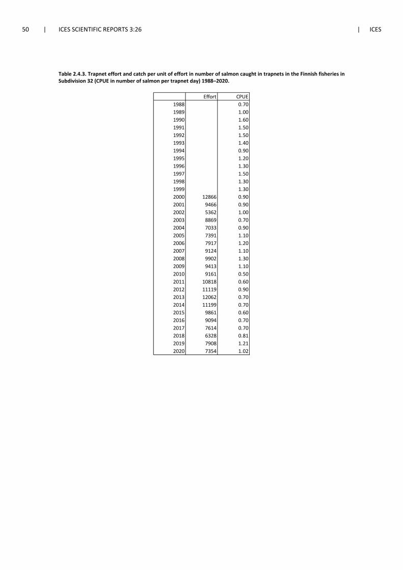
50 | ICES SCIENTIFIC REPORTS 3:26 | ICES
Table 2.4.3. Trapnet effort and catch per unit of effort in number of salmon caught in trapnets in the Finnish fisheries in Subdivision 32 (CPUE in number of salmon per trapnet day) 1988–2020.
Effort CPUE1988 0.701989 1.001990 1.601991 1.501992 1.501993 1.401994 0.901995 1.201996 1.301997 1.501998 1.301999 1.302000 12866 0.902001 9466 0.902002 5362 1.002003 8869 0.702004 7033 0.902005 7391 1.102006 7917 1.202007 9124 1.102008 9902 1.302009 9413 1.102010 9161 0.502011 10818 0.602012 11119 0.902013 12062 0.702014 11199 0.702015 9861 0.602016 9094 0.702017 7614 0.702018 6328 0.812019 7908 1.212020 7354 1.02
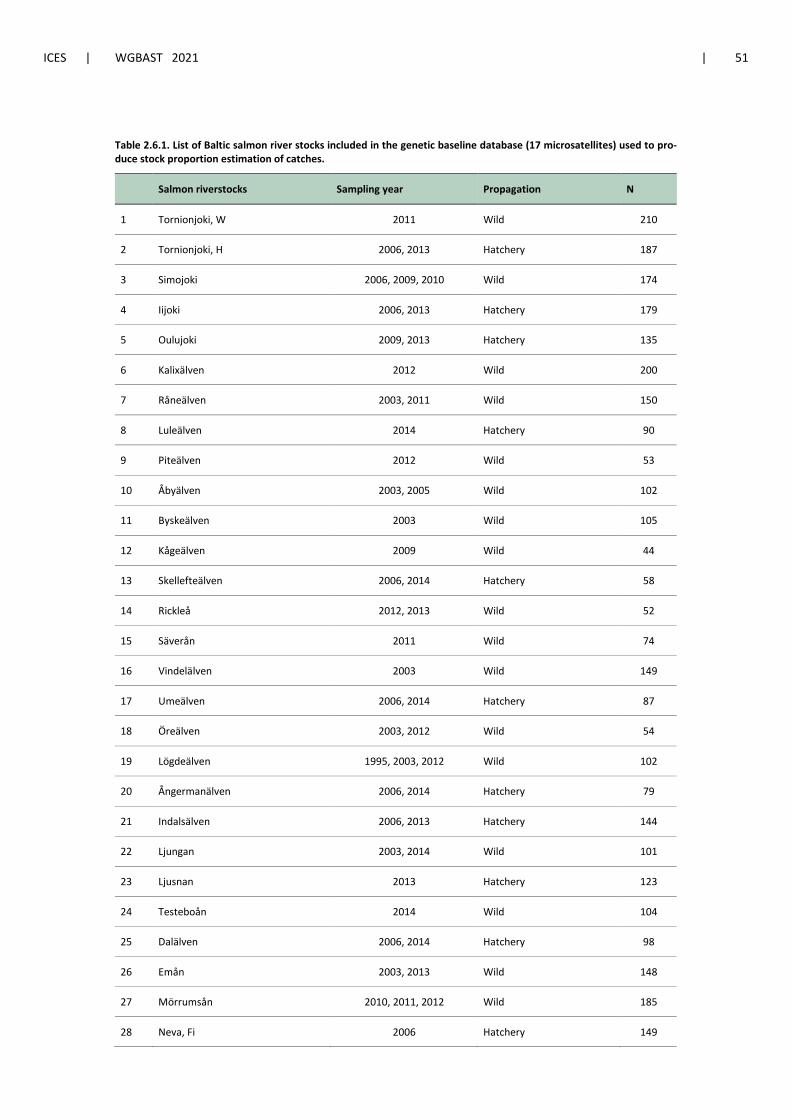
ICES | WGBAST 2021 | 51
Table 2.6.1. List of Baltic salmon river stocks included in the genetic baseline database (17 microsatellites) used to pro-duce stock proportion estimation of catches.
Salmon riverstocks Sampling year Propagation N
1 Tornionjoki, W 2011 Wild 210
2 Tornionjoki, H 2006, 2013 Hatchery 187
3 Simojoki 2006, 2009, 2010 Wild 174
4 Iijoki 2006, 2013 Hatchery 179
5 Oulujoki 2009, 2013 Hatchery 135
6 Kalixälven 2012 Wild 200
7 Råneälven 2003, 2011 Wild 150
8 Luleälven 2014 Hatchery 90
9 Piteälven 2012 Wild 53
10 Åbyälven 2003, 2005 Wild 102
11 Byskeälven 2003 Wild 105
12 Kågeälven 2009 Wild 44
13 Skellefteälven 2006, 2014 Hatchery 58
14 Rickleå 2012, 2013 Wild 52
15 Säverån 2011 Wild 74
16 Vindelälven 2003 Wild 149
17 Umeälven 2006, 2014 Hatchery 87
18 Öreälven 2003, 2012 Wild 54
19 Lögdeälven 1995, 2003, 2012 Wild 102
20 Ångermanälven 2006, 2014 Hatchery 79
21 Indalsälven 2006, 2013 Hatchery 144
22 Ljungan 2003, 2014 Wild 101
23 Ljusnan 2013 Hatchery 123
24 Testeboån 2014 Wild 104
25 Dalälven 2006, 2014 Hatchery 98
26 Emån 2003, 2013 Wild 148
27 Mörrumsån 2010, 2011, 2012 Wild 185
28 Neva, Fi 2006 Hatchery 149
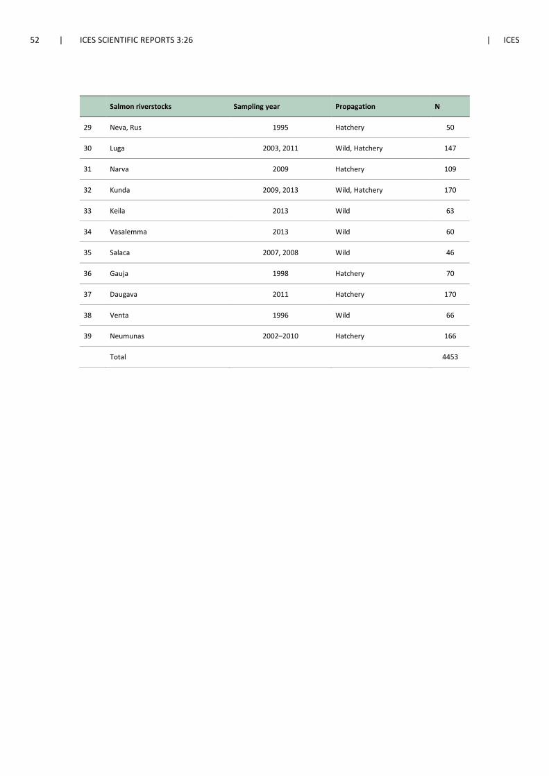
52 | ICES SCIENTIFIC REPORTS 3:26 | ICES
Salmon riverstocks Sampling year Propagation N
29 Neva, Rus 1995 Hatchery 50
30 Luga 2003, 2011 Wild, Hatchery 147
31 Narva 2009 Hatchery 109
32 Kunda 2009, 2013 Wild, Hatchery 170
33 Keila 2013 Wild 63
34 Vasalemma 2013 Wild 60
35 Salaca 2007, 2008 Wild 46
36 Gauja 1998 Hatchery 70
37 Daugava 2011 Hatchery 170
38 Venta 1996 Wild 66
39 Neumunas 2002–2010 Hatchery 166
Total
4453
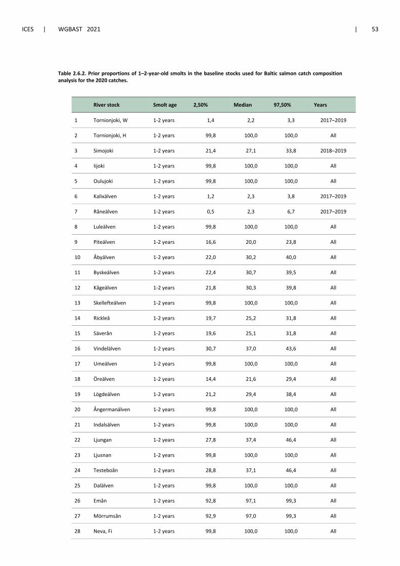
ICES | WGBAST 2021 | 53
Table 2.6.2. Prior proportions of 1–2-year-old smolts in the baseline stocks used for Baltic salmon catch composition analysis for the 2020 catches.
River stock Smolt age 2,50% Median 97,50% Years
1 Tornionjoki, W 1-2 years 1,4 2,2 3,3 2017–2019
2 Tornionjoki, H 1-2 years 99,8 100,0 100,0 All
3 Simojoki 1-2 years 21,4 27,1 33,8 2018–2019
4 Iijoki 1-2 years 99,8 100,0 100,0 All
5 Oulujoki 1-2 years 99,8 100,0 100,0 All
6 Kalixälven 1-2 years 1,2 2,3 3,8 2017–2019
7 Råneälven 1-2 years 0,5 2,3 6,7 2017–2019
8 Luleälven 1-2 years 99,8 100,0 100,0 All
9 Piteälven 1-2 years 16,6 20,0 23,8 All
10 Åbyälven 1-2 years 22,0 30,2 40,0 All
11 Byskeälven 1-2 years 22,4 30,7 39,5 All
12 Kågeälven 1-2 years 21,8 30,3 39,8 All
13 Skellefteälven 1-2 years 99,8 100,0 100,0 All
14 Rickleå 1-2 years 19,7 25,2 31,8 All
15 Säverån 1-2 years 19,6 25,1 31,8 All
16 Vindelälven 1-2 years 30,7 37,0 43,6 All
17 Umeälven 1-2 years 99,8 100,0 100,0 All
18 Öreälven 1-2 years 14,4 21,6 29,4 All
19 Lögdeälven 1-2 years 21,2 29,4 38,4 All
20 Ångermanälven 1-2 years 99,8 100,0 100,0 All
21 Indalsälven 1-2 years 99,8 100,0 100,0 All
22 Ljungan 1-2 years 27,8 37,4 46,4 All
23 Ljusnan 1-2 years 99,8 100,0 100,0 All
24 Testeboån 1-2 years 28,8 37,1 46,4 All
25 Dalälven 1-2 years 99,8 100,0 100,0 All
26 Emån 1-2 years 92,8 97,1 99,3 All
27 Mörrumsån 1-2 years 92,9 97,0 99,3 All
28 Neva, Fi 1-2 years 99,8 100,0 100,0 All
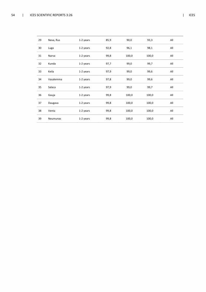
54 | ICES SCIENTIFIC REPORTS 3:26 | ICES
29 Neva, Rus 1-2 years 85,9 90,0 93,3 All
30 Luga 1-2 years 92,8 96,1 98,1 All
31 Narva 1-2 years 99,8 100,0 100,0 All
32 Kunda 1-2 years 97,7 99,0 99,7 All
33 Keila 1-2 years 97,9 99,0 99,6 All
34 Vasalemma 1-2 years 97,8 99,0 99,6 All
35 Salaca 1-2 years 97,9 99,0 99,7 All
36 Gauja 1-2 years 99,8 100,0 100,0 All
37 Daugava 1-2 years 99,8 100,0 100,0 All
38 Venta 1-2 years 99,8 100,0 100,0 All
39 Neumunas 1-2 years 99,8 100,0 100,0 All
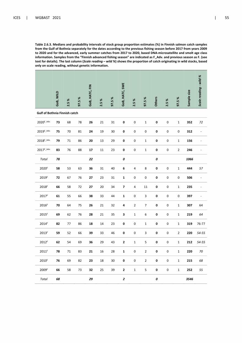
ICES | WGBAST 2021 | 55
Table 2.6.3. Medians and probability intervals of stock group proportion estimates (%) in Finnish salmon catch samples from the Gulf of Bothnia separately for the dates according to the previous fishing season before 2017 from years 2009 to 2020 and for the advanced, early summer catches from 2017 to 2020, based DNA-microsatellite and smolt age class information. Samples from the “Finnish advanced fishing season” are indicated as F_Adv. and previous season as F. (see text for details). The last column (Scale reading – wild %) shows the proportion of catch originating in wild stocks, based only on scale reading, without genetic information.
GoB
, WIL
D
2.5
%
97.5
%
GoB
, HAT
C, F
IN
2.5
%
97.5
%
GoB
, HAT
C, S
WE
2.5
%
97.5
%
Oth
ers
2.5
%
97.5
%
Sam
ple
size
Scal
e re
adin
g - w
ild %
Gulf of Bothnia Finnish catch
2020F_Adv. 73 68 78 26 21 31 0 0 1 0 0 1 352 72
2019F_Adv. 75 70 81 24 19 30 0 0 0 0 0 0 312 -
2018F_Adv. 79 71 86 20 13 29 0 0 1 0 0 1 156 -
2017F_Adv. 83 76 88 17 11 23 0 0 1 0 0 2 246 -
Total 78 22 0 0 1066
2020F 58 53 63 36 31 40 6 4 8 0 0 1 444 57
2019F 72 67 76 27 23 31 1 0 0 0 0 0 506 -
2018F 66 58 72 27 20 34 7 4 11 0 0 1 235 -
2017F 61 55 66 38 33 44 1 0 3 0 0 0 397 -
2016F 70 64 75 26 21 32 4 2 7 0 0 1 307 64
2015F 69 62 76 28 21 35 3 1 6 0 0 1 219 64
2014F 82 77 86 18 14 23 0 0 1 0 0 1 319 76-77
2013F 59 52 66 39 33 46 0 0 3 0 0 2 220 54-55
2012F 62 54 69 36 29 43 2 1 5 0 0 1 212 54-55
2011F 78 71 83 21 16 28 1 0 2 0 0 1 220 70
2010F 76 69 82 23 18 30 0 0 2 0 0 1 215 68
2009F 66 58 73 32 25 39 2 1 5 0 0 1 252 55
Total 68 29 2 0 3546
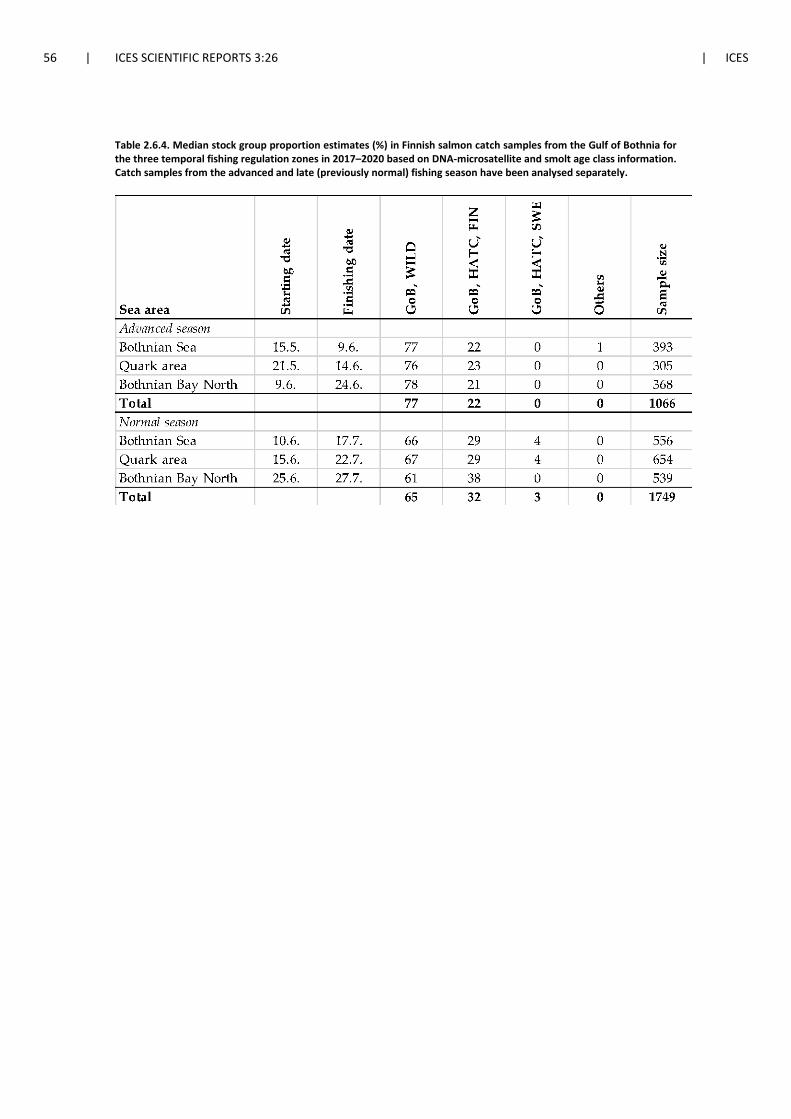
56 | ICES SCIENTIFIC REPORTS 3:26 | ICES
Table 2.6.4. Median stock group proportion estimates (%) in Finnish salmon catch samples from the Gulf of Bothnia for the three temporal fishing regulation zones in 2017–2020 based on DNA-microsatellite and smolt age class information. Catch samples from the advanced and late (previously normal) fishing season have been analysed separately.
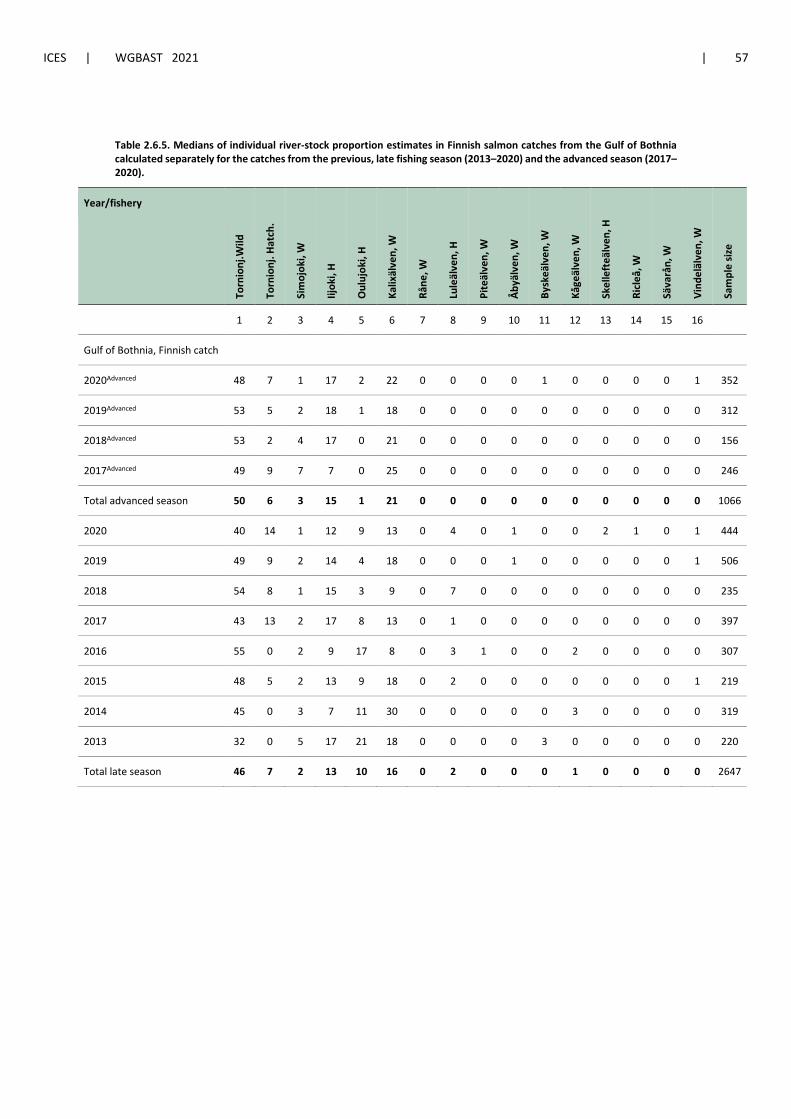
ICES | WGBAST 2021 | 57
Table 2.6.5. Medians of individual river-stock proportion estimates in Finnish salmon catches from the Gulf of Bothnia calculated separately for the catches from the previous, late fishing season (2013–2020) and the advanced season (2017–2020).
Year/fishery
Torn
ionj
.Wild
Torn
ionj
. Hat
ch.
Sim
ojok
i, W
Iijok
i, H
Oul
ujok
i, H
Kalix
älve
n, W
Råne
, W
Lule
älve
n, H
Pite
älve
n, W
Åbyä
lven
, W
Bysk
eälv
en, W
Kåge
älve
n, W
Skel
left
eälv
en, H
Ricl
eå, W
Säva
rån,
W
Vind
eläl
ven,
W
Sam
ple
size
1 2 3 4 5 6 7 8 9 10 11 12 13 14 15 16
Gulf of Bothnia, Finnish catch
2020Advanced 48 7 1 17 2 22 0 0 0 0 1 0 0 0 0 1 352
2019Advanced 53 5 2 18 1 18 0 0 0 0 0 0 0 0 0 0 312
2018Advanced 53 2 4 17 0 21 0 0 0 0 0 0 0 0 0 0 156
2017Advanced 49 9 7 7 0 25 0 0 0 0 0 0 0 0 0 0 246
Total advanced season 50 6 3 15 1 21 0 0 0 0 0 0 0 0 0 0 1066
2020 40 14 1 12 9 13 0 4 0 1 0 0 2 1 0 1 444
2019 49 9 2 14 4 18 0 0 0 1 0 0 0 0 0 1 506
2018 54 8 1 15 3 9 0 7 0 0 0 0 0 0 0 0 235
2017 43 13 2 17 8 13 0 1 0 0 0 0 0 0 0 0 397
2016 55 0 2 9 17 8 0 3 1 0 0 2 0 0 0 0 307
2015 48 5 2 13 9 18 0 2 0 0 0 0 0 0 0 1 219
2014 45 0 3 7 11 30 0 0 0 0 0 3 0 0 0 0 319
2013 32 0 5 17 21 18 0 0 0 0 3 0 0 0 0 0 220
Total late season 46 7 2 13 10 16 0 2 0 0 0 1 0 0 0 0 2647
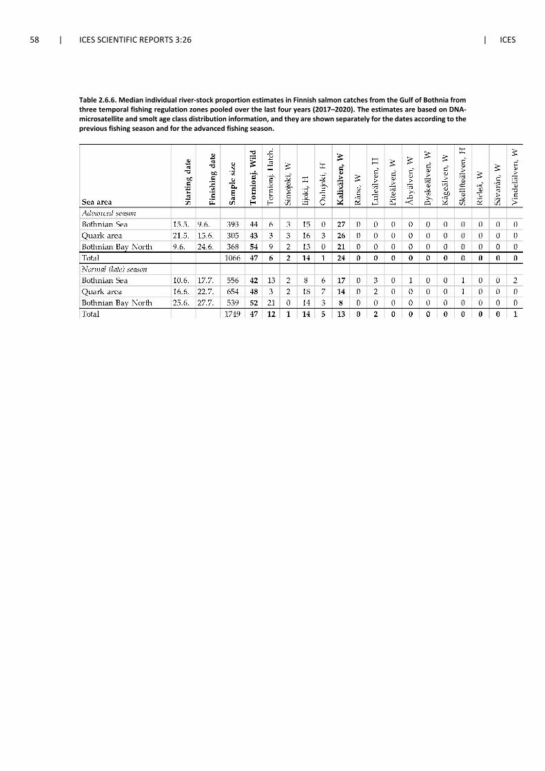
58 | ICES SCIENTIFIC REPORTS 3:26 | ICES
Table 2.6.6. Median individual river-stock proportion estimates in Finnish salmon catches from the Gulf of Bothnia from three temporal fishing regulation zones pooled over the last four years (2017–2020). The estimates are based on DNA-microsatellite and smolt age class distribution information, and they are shown separately for the dates according to the previous fishing season and for the advanced fishing season.
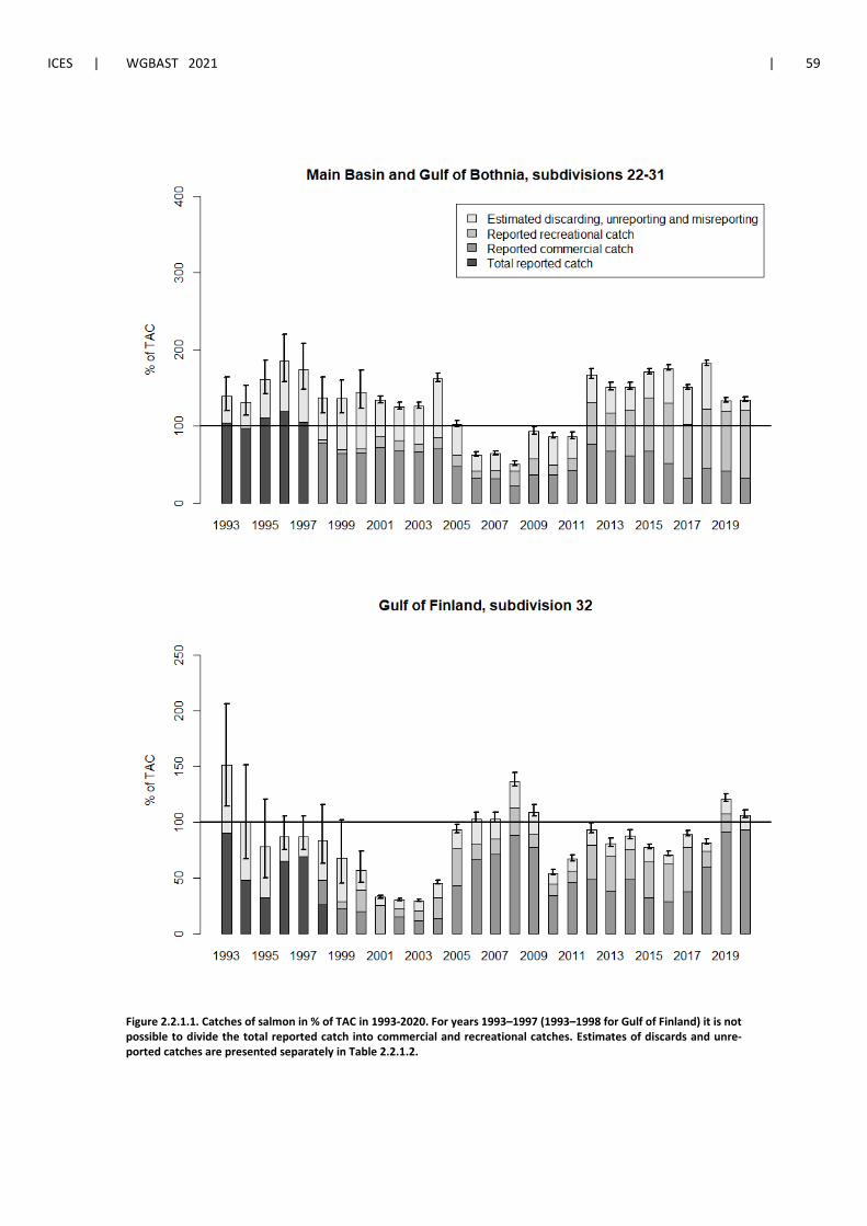
ICES | WGBAST 2021 | 59
Figure 2.2.1.1. Catches of salmon in % of TAC in 1993-2020. For years 1993–1997 (1993–1998 for Gulf of Finland) it is not possible to divide the total reported catch into commercial and recreational catches. Estimates of discards and unre-ported catches are presented separately in Table 2.2.1.2.
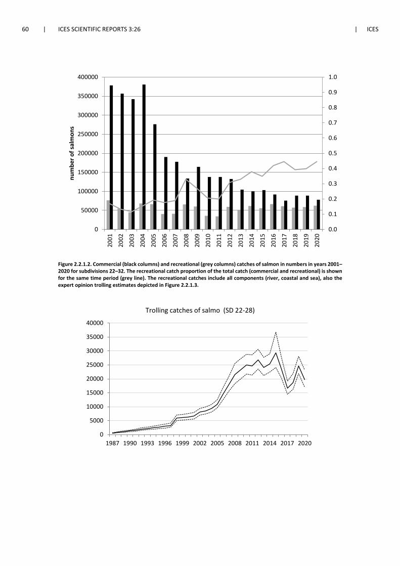
60 | ICES SCIENTIFIC REPORTS 3:26 | ICES
Figure 2.2.1.2. Commercial (black columns) and recreational (grey columns) catches of salmon in numbers in years 2001–2020 for subdivisions 22–32. The recreational catch proportion of the total catch (commercial and recreational) is shown for the same time period (grey line). The recreational catches include all components (river, coastal and sea), also the expert opinion trolling estimates depicted in Figure 2.2.1.3.
0.0
0.1
0.2
0.3
0.4
0.5
0.6
0.7
0.8
0.9
1.0
0
50000
100000
150000
200000
250000
300000
350000
400000
2001
2002
2003
2004
2005
2006
2007
2008
2009
2010
2011
2012
2013
2014
2015
2016
2017
2018
2019
2020
num
ber o
f sal
mon
s
0
5000
10000
15000
20000
25000
30000
35000
40000
1987 1990 1993 1996 1999 2002 2005 2008 2011 2014 2017 2020
Trolling catches of salmo (SD 22-28)
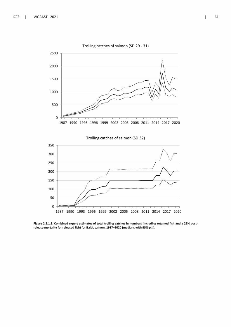
ICES | WGBAST 2021 | 61
Figure 2.2.1.3. Combined expert estimates of total trolling catches in numbers (including retained fish and a 25% post-release mortality for released fish) for Baltic salmon, 1987–2020 (medians with 95% p.i.).
0
500
1000
1500
2000
2500
1987 1990 1993 1996 1999 2002 2005 2008 2011 2014 2017 2020
Trolling catches of salmon (SD 29 - 31)
0
50
100
150
200
250
300
350
1987 1990 1993 1996 1999 2002 2005 2008 2011 2014 2017 2020
Trolling catches of salmon (SD 32)
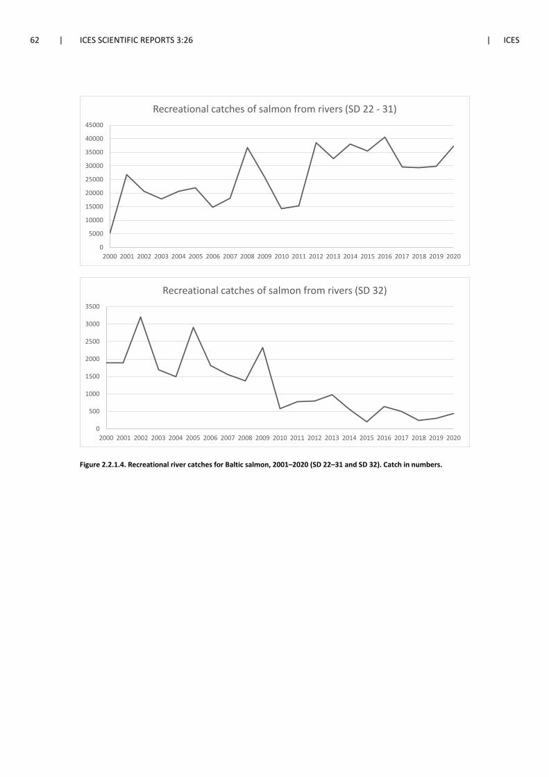
62 | ICES SCIENTIFIC REPORTS 3:26 | ICES
Figure 2.2.1.4. Recreational river catches for Baltic salmon, 2001–2020 (SD 22–31 and SD 32). Catch in numbers.
0
5000
10000
15000
20000
25000
30000
35000
40000
45000
2000 2001 2002 2003 2004 2005 2006 2007 2008 2009 2010 2011 2012 2013 2014 2015 2016 2017 2018 2019 2020
Recreational catches of salmon from rivers (SD 22 - 31)
0
500
1000
1500
2000
2500
3000
3500
2000 2001 2002 2003 2004 2005 2006 2007 2008 2009 2010 2011 2012 2013 2014 2015 2016 2017 2018 2019 2020
Recreational catches of salmon from rivers (SD 32)
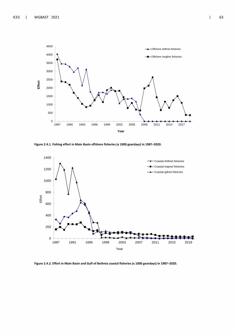
ICES | WGBAST 2021 | 63
Figure 2.4.1. Fishing effort in Main Basin offshore fisheries (x 1000 geardays) in 1987–2020.
Figure 2.4.2. Effort in Main Basin and Gulf of Bothnia coastal fisheries (x 1000 geardays) in 1987–2020.
0
500
1000
1500
2000
2500
3000
3500
4000
4500
1987 1990 1993 1996 1999 2002 2005 2008 2011 2014 2017
Effo
rt
Year
Offshore driftnet fisheries
Offshore longline fisheries
0
200
400
600
800
1000
1200
1400
1987 1991 1995 1999 2003 2007 2011 2015 2019
Effo
rt
Year
Coastal driftnet fisheries
Coastal trapnet fisheries
Coastal gillnet fisheries
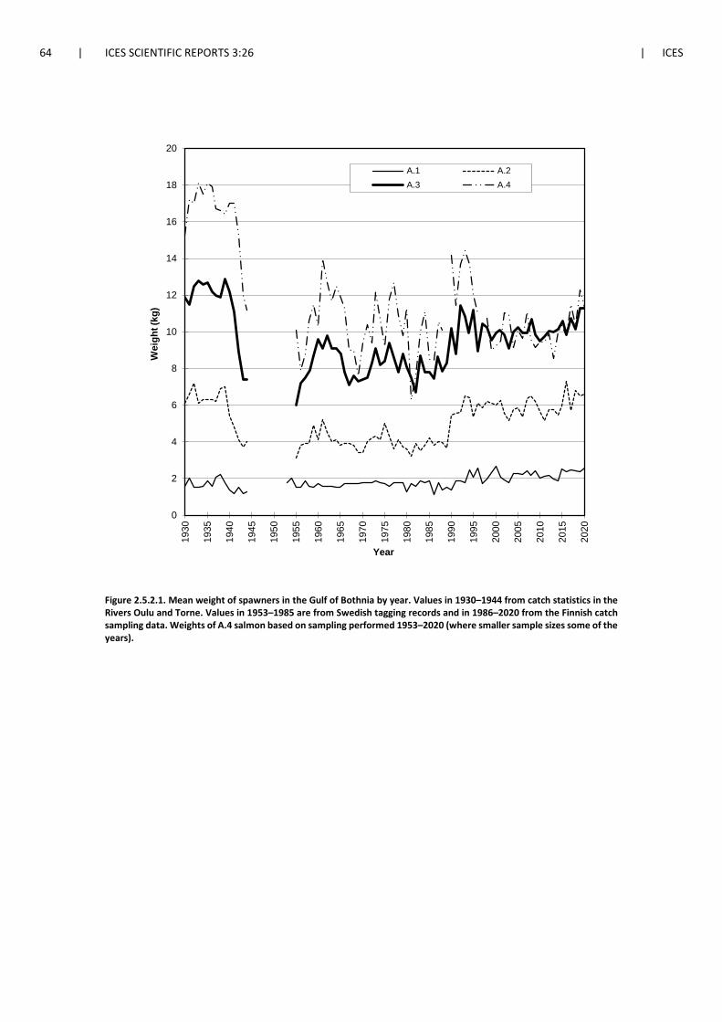
64 | ICES SCIENTIFIC REPORTS 3:26 | ICES
Figure 2.5.2.1. Mean weight of spawners in the Gulf of Bothnia by year. Values in 1930–1944 from catch statistics in the Rivers Oulu and Torne. Values in 1953–1985 are from Swedish tagging records and in 1986–2020 from the Finnish catch sampling data. Weights of A.4 salmon based on sampling performed 1953–2020 (where smaller sample sizes some of the years).
0
2
4
6
8
10
12
14
16
18
20
1930
1935
1940
1945
1950
1955
1960
1965
1970
1975
1980
1985
1990
1995
2000
2005
2010
2015
2020
Wei
ght (
kg)
Year
A.1 A.2A.3 A.4
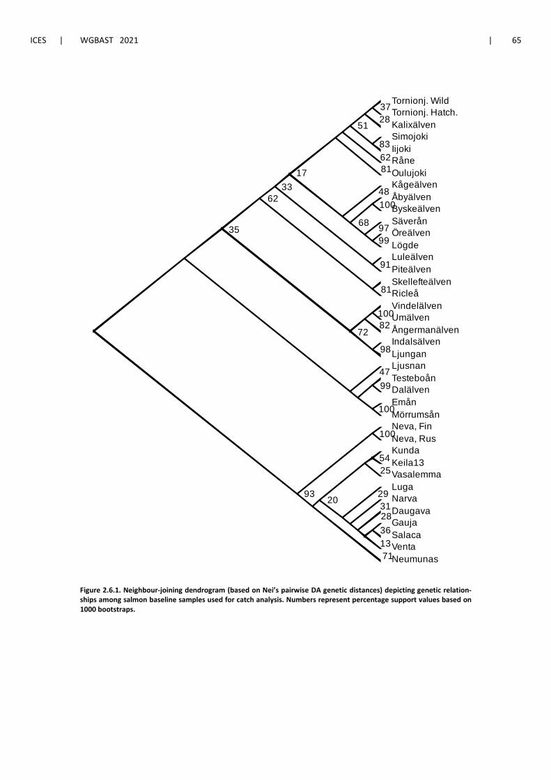
ICES | WGBAST 2021 | 65
Figure 2.6.1. Neighbour-joining dendrogram (based on Nei’s pairwise DA genetic distances) depicting genetic relation-ships among salmon baseline samples used for catch analysis. Numbers represent percentage support values based on 1000 bootstraps.
Tornionj. Wild Tornionj. Hatch. 37
Kalixälven 28
Simojoki Iijoki 83
51
Råne 62 Oulujoki 81 Kågeälven Åbyälven Byskeälven 100
Säverån Öreälven Lögde99
9768
48
17
Luleälven Piteälven 91
33
Skellefteälven Ricleå 81
62
Vindelälven Umälven100
Ångermanälven 82
Indalsälven Ljungan 98
72
35
Ljusnan Testeboån Dalälven 99
Emån Mörrumsån100
47
Neva, Fin Neva, Rus 100
Kunda Keila1354
Vasalemma25
Luga Narva Daugava Gauja Salaca36
Venta13
28312920
Neumunas71
93
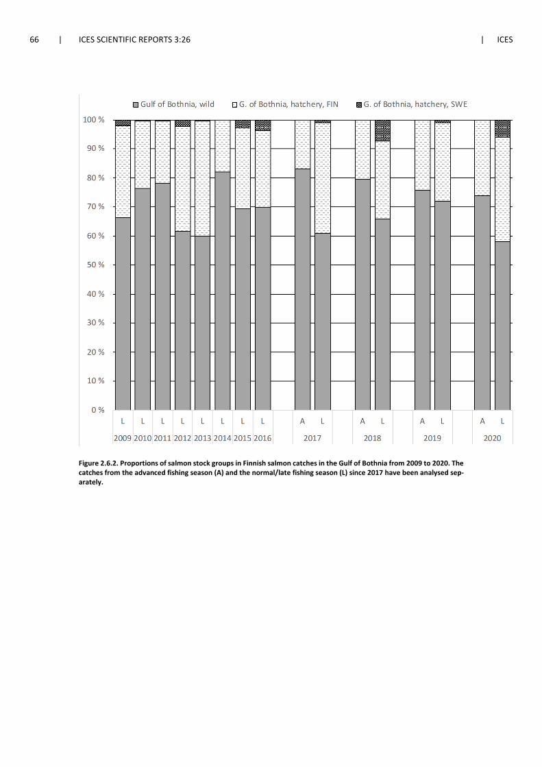
66 | ICES SCIENTIFIC REPORTS 3:26 | ICES
Figure 2.6.2. Proportions of salmon stock groups in Finnish salmon catches in the Gulf of Bothnia from 2009 to 2020. The catches from the advanced fishing season (A) and the normal/late fishing season (L) since 2017 have been analysed sep-arately.
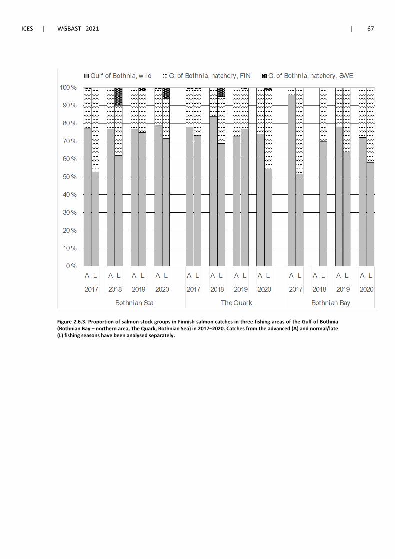
ICES | WGBAST 2021 | 67
Figure 2.6.3. Proportion of salmon stock groups in Finnish salmon catches in three fishing areas of the Gulf of Bothnia (Bothnian Bay – northern area, The Quark, Bothnian Sea) in 2017–2020. Catches from the advanced (A) and normal/late (L) fishing seasons have been analysed separately.
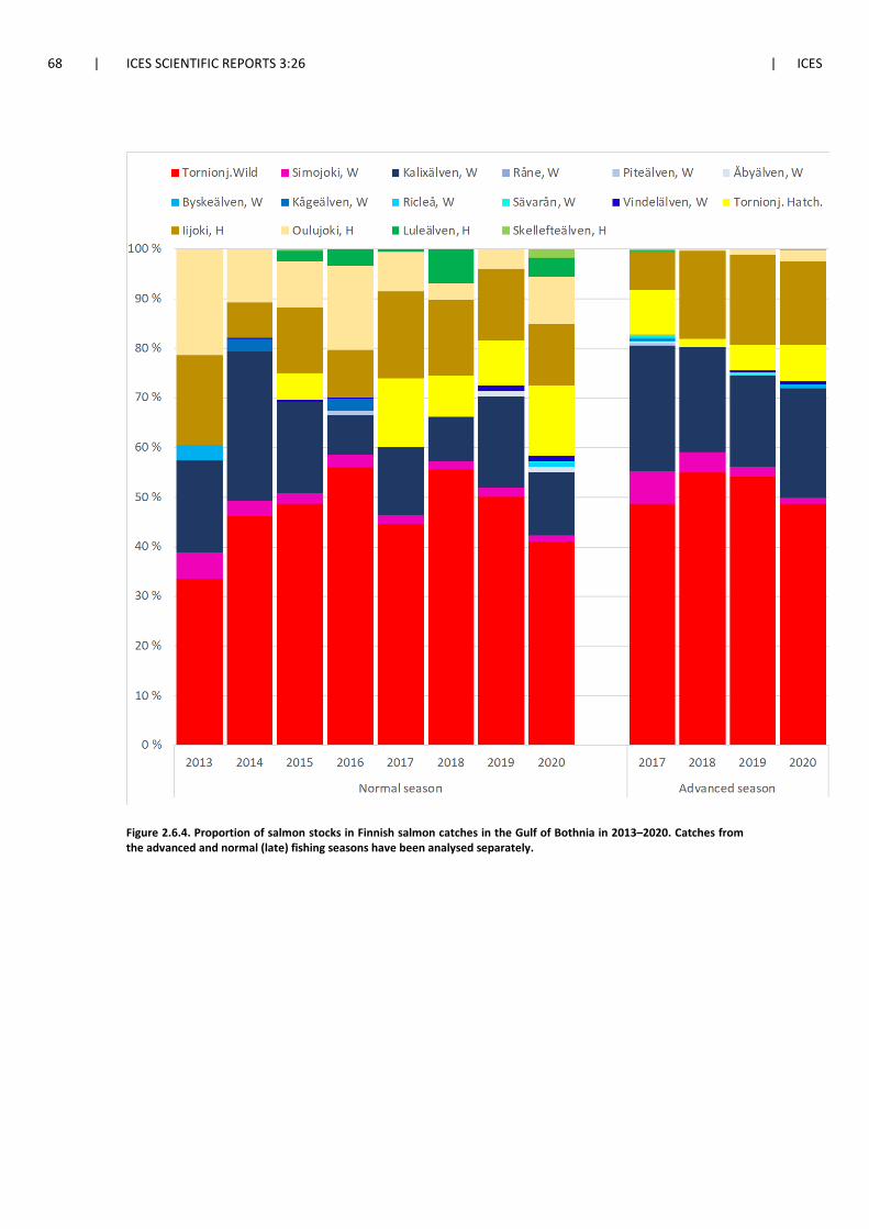
68 | ICES SCIENTIFIC REPORTS 3:26 | ICES
Figure 2.6.4. Proportion of salmon stocks in Finnish salmon catches in the Gulf of Bothnia in 2013–2020. Catches from the advanced and normal (late) fishing seasons have been analysed separately.
ICES | WGBAST 2021 | 69
3 River data on salmon populations
The Baltic salmon rivers are divided into four main categories: wild, mixed, reared and poten-tial. Details on how rivers in countries and assessment units (AUs) are classified into these four river categories are given in the Stock Annex (Annex 2). At present there are 58 salmon rivers out of which 27, 14 and 17 are considered as wild, mixed (i.e. with both natural and reared pro-duction) and reared, respectively. In addition, there currently exist 21 potential salmon rivers in five countries (Section 3.2).
Over the years, some rivers have received altered status and further changes are likely to occur in the future. For example, in 2013 and 2014 the formerly potential salmon rivers Testeboån (AU 3) and Kågeälven (AU 2) in Sweden received status as wild, as they had fulfilled criteria previously set up by WGBAST (ICES, 2008c). Among the 14 rivers currently classified as mixed, the present level of salmon releases in Estonian rivers Pirita and Väänä (AU 6) are already close to the threshold of less than 10% reared smolt production adopted by WGBAST as a criteria for wild rivers (Annex 2, Table A.1.2.1). Hence, if stocking would be further reduced or stopped, these rivers could become candidates for receiving wild status by WGBAST. Conversely, the previously wild river Pärnu in Estonia (AU 5) was listed in 2018 as mixed, because of an ongoing restoration programme that includes substantial annual releases of hatchery-reared juveniles (ICES, 2018a; 2018b). In the coming years, WGBAST plans to review its criteria and update the list of wild, mixed, and potential salmon rivers, according to river specific information, new studies and internationally recognized recommendations.
3.1 Wild salmon populations in Main Basin and Gulf of Bothnia
Current wild salmon rivers in Main Basin and Gulf of Bothnia are listed per country and assess-ment unit in the Stock Annex (Annex 2).
3.1.1 Rivers in assessment unit 1 (Gulf of Bothnia, SD 31)
River catches and fishery In 2012, the catch in Tornionjoki was three times higher than in 2011 and for the first time since the beginning of the time-series with annual catch statistics, it exceeded 100 tonnes (Table 3.1.1.1). In 2014, the catch increased to 147 tonnes, and in 2016 it reached the present record of 161 tonnes (Table 3.1.1.1). In 2017 and 2018, the catch again declined to around 90 tonnes, but in 2019 and 2020 it increased again, and was 111 and 130 tonnes, respectively. Catch levels similar to those observed in 2012–2020 were observed in the early 20th century (Figure 3.1.1.1). Salmon catches in Simojoki did not rise much in 2012–2013, which is partly due to a low fishing effort. However, in 2014 and 2015 there was a clear increase in the catch and the rising trend continued until 2016, when the catch was 1.8 tonnes (Table 3.1.1.1). As in Tornionjoki, 2017 catches dropped also in Simojoki, and they have been between 0.5–1 tonnes in 2017–2019 but increased again in 2020 to 1.5 tonnes. The catches in Kalixälven have decreased in later years mostly depending on not functional catch reporting system and they do not correspond to the registered number of salmon that have passed the fishway, totally 250 salmon were caught and out of which 100 were retained.
A special kind of fishing from boat (rod fishing by rowing) dominates the salmon fishing in Tor-nionjoki. This type of fishing also occurs in Kalixälven, but there it is not as dominating as in
70 | ICES SCIENTIFIC REPORTS 3:26 | ICES
Tornionjoki. CPUE of this fishery in Tornionjoki has increased tens of times since the late 1980s (Table 3.1.1.1), apparently reflecting the parallel increase in the abundance of spawners in the river. The CPUE has been high (over 1000 grams/fishing day) in 1997, 2008 and 2012–2016, when the total river catches were also peaking. In 2017 CPUE dropped to 860 g/day. In 2018, it in-creased to 1200 g/day and in 2019 and 2020 the CPUE was 970 g/day and 930 g/day, respectively. Annual changes in CPUE and in total river catch generally follow each other. However, in 2019 and 2020 the CPUE was exceptionally low compared to the total catch.
In Råneälven, the local administration has since 2014 utilized a seasonal catch bag limit regula-tion of maximum of three salmon per person and season. Both obligatory tagging of killed fish (maximum of three tags per person and year) and a digital catch reporting system has been uti-lized to aid in enforcement. Most (80–90%) of the salmon caught with rod are released back; in 2017 a total of 56 salmon were caught, out of which 45 were released, whereas in 2018 only two salmon were caught and tagged (retained). The catch in 2019 was 45 salmon out of which seven were tagged and retained; in 2020 only two salmon were caught and retained.
Spawning runs and their composition In Kalixälven salmon are counted in the fishway at the waterfall in Jockfall about 100 km from the river mouth. From 2007 to 2012 the mean annual run was 5500 salmon. In 2013, the run in-creased to the highest observed when more than 15 000 salmon passed the fishway. The counted runs in 2014–2019 stayed at a lower level (between 5000–10 000 salmon). In 2020, nearly 19 000 were registered in the fishcounter (Table 3.1.1.2). Yearly very few reared (adipose finclipped) salmon has been registered in the fish counter. Between 2015 to 2018 no reared salmon was reg-istered in the counter. In 2019, six reared salmon was registered of 9957 salmon, and in 2020 only one salmon with clipped adipose fin was registered of 18 664which results in very low propor-tion of strayers.
A hydroacoustic split-beam technique was employed in 2003–2007 to count the spawning run in Simojoki. It seems evident that these counts covered only a fraction of the total run, as there are irregularities in the river bottom at the counting site, allowing salmon to pass without being recorded. Since 2008, the split-beam technique has been replaced by an echosounder called DID-SON (Dual frequency IDentification SONar) and in 2020 a new generation version of DIDSON (called ARIS) replaced DIDSON. According to monitoring results, the seasonal run size has ranged from less than 1000 up to more than 5000 fish (Table 3.1.1.2). Spawning runs gradually increased from 2004 to 2008–2009, but again dropped in 2010–2011. In 2012, the run increased fourfold from the previous year (to about 3000) and also the runs in 2013–2015 were about as abundant (3000–4000 salmon). The 2016 run was record-high with 5400 salmon counted. In 2017, the run dropped below 2000 salmon but increased in 2018, 2019 and 2020 to about 4000 salmon/year (Table 3.1.1.2). A lot of back-and-forth movement of salmon has been detected in Simojoki, especially in 2018, which erodes the accuracy of the counts. There have also been prob-lems connected to the separation of species.
The spawning runs into Tornionjoki have also been monitored using the DIDSON technique since 2009, but in 2019 the old DIDSON units were replaced by ARIS sonars. The observed sea-sonal run size has ranged from 17 200 (year 2010) to 100 200 (year 2014) salmon (Table 3.1.1.2). Grilse account for a minority (7–24%) of the annual spawning runs. The run size in 2016 (98 300 salmon) was almost as high as in the record year 2014 (101 000 salmon), but as in the Simojoki, the run again dropped in 2017 (to about 41 000 salmon). In 2018 the counted amount increased only slightly (to 47 000 salmon), but in 2019 and 2020 the total count increased further, to 65 500 and 69 100 salmon, respectively.
The Tornionjoki counting site is located about 100 km upstream from the river mouth. Therefore, salmon which are either caught below the site or stay to spawn below the site must be assessed
ICES | WGBAST 2021 | 71
and added into the hydroacoustic count, in order to get an estimate of the total run size into the river (Lilja et al., 2010). Also, according to auxiliary studies, a small fraction of the spawners pass the counting site via the fast-flowing mid-channel without being detected by sonars. The mid-channel seems to be utilised the more by salmon the lower the river water level is (Isometsä et al., 2021). The 2018 and 2019 counts probably represents a smaller-than-normal proportion of the total run size into the river; observations were made of unusually high amounts of salmon stay-ing on the lowermost river until autumn 2018. Moreover, the very low prevailing water level in 2018 and 2019 probably allowed many spawners to pass the hydroacoustic counter via the deep-est mid-channel where they may have remained undetected.
In 2014–2019, the spawning run in Råneälven has been monitored with an ultra-sound camera (SIMSONAR). The technique is similar to that used in Tornionjoki and Simojoki. The counting site is located about 35 km upstream from the river mouth, and the counts are expected to rep-resent the total run as almost no salmon spawning areas exist downstream. The total counted salmon runs in the period 2014–2019 has varied between 1000–4000 and in 2020 the salmon run was 2461 (Table 3.1.1.3).
Over 13 000 catch samples have been collected from the Tornionjoki salmon fishery since the mid-1970s. Table 3.1.1.3 shows sample size, sea age composition, sex composition and propor-tion of reared fish (identified either by the absence of adipose fin or by scale reading) of the data for the given time periods. Caught fish have generally become older, and the proportion of repeat spawners has increased in parallel with a decreasing sea fishing pressure (see Section 4). The strong spawning runs into Tornionjoki in 2012–2016 were a result of fish from several smolt co-horts. In these years, the proportion of females has been fairly stable, about two thirds of total biomass, but in 2018 and 2019 only about 55% of the total biomass were females. The proportion of repeat spawners has generally been between 5–10% during the last decade. However, a record high proportion of repeat spawners (14%) was observed in 2014, and the proportion was high also in 2018 and 2020 (12% and 11%, respectively). On the contrary, in 2017 and 2019 the propor-tion of repeat spawners was only 3%, indicating large interannual variation. Very few salmon of reared origin (<1%) have been observed in the Tornionjoki catch samples in the last decade (Table 3.1.1.3).
Parr densities and smolt trapping The lowest parr densities in AU 1 rivers were observed in the mid-1980s (Table 3.1.1.4, Figures 3.1.1.4 and 3.1.1.5). During the 1990s, densities increased in a cyclic pattern with two ‘jumps’. The second, higher jump started in 1996–1997. Between these increases there was a collapse in densities around the mid-1990s, when also the highest M74 mortality was observed (see below). Average parr densities are nowadays 5–60 times higher than in the mid-1980s. Since the turn of the millennium, annual parr densities have varied 2–6 fold. In Simojoki, some years with higher-than-earlier densities of 0+ parr have been observed recently, but annual variation has been large and densities of older parr have often not increased in this river after years with high 0+ densities. In the other AU 1 rivers, however, parr densities of all ages have continued to increase rather steadily until in the mid-2010s.
In some years, like in 2003, high densities of parr hatched in Simojoki, Tornionjoki and Kalixäl-ven despite relatively low preceding river catches (indicating low spawner abundance). Simi-larly, high densities of 0+ parr were observed in Tornionjoki in 2008 and 2011, although river catches and spawners counts in the preceding years were not among the highest. Possible rea-sons for this inconsistency include exceptionally warm and low summer-time river water, which might have affected fishing success in the river and even measurements of parr densities. In years 2006, 2013, 2014, 2018 and 2019 conditions for electrofishing were favourable because of very low river water levels, whereas they were the opposite in 2004 and 2005. These kinds of
72 | ICES SCIENTIFIC REPORTS 3:26 | ICES
changes in electrofishing conditions may have affected the results, and one must therefore be somewhat cautious when interpreting the data obtained.
In Simojoki, the mean density of one-summer old parr increased by about 50% from 2015 to 2016 and it continued to increase in 2017 (Table 3.1.1.4). The 2019 density of 0+ parr (40.9 ind./100 sqm) is record high in the time-series, although most of the uppermost sites still lack 0+ parr. In 2020 the 0+ parr density dropped to about half (21.3 ind./100 sqm) of that of 2019, although the number of spawners giving rise to these parr densities was almost identical (Table 3.1.1.2). The density of older parr increased rapidly from 2015 (6.5 ind./100 sqm) to a record high level in 2018 (42 ind./100 sqm). In 2019, however, the density dropped to 14.4 ind./100 sqm and in 2020 the density increased to 19.9 ind./100 sqm. In Tornionjoki the densities of 0+ parr in 2014 and 2015 were clearly higher than in any earlier year in the time-series. In 2016, the average density of 0+ parr on the sampled sites was somewhat lower than in 2015. Several flood peaks due to heavy rains prevented electrofishing on the lower and on some of the middle and upper sections of the river system. In 2017, the average density of 0+ parr increased and was the third highest in the time-series (28.5 ind./100 sqm). In 2018 the mean 0+ parr density again dropped to only 18.3 ind./100 sqm, however in 2019 and 2020 the densities were higher: 25.5 and 20.5 ind./100 sqm, respectively. The average density of older parr in 2017 (17.2 ind./100 m2) dropped from the two earlier years and in 2019 a further decrease (to 15.2 ind./100 sqm) was observed, but there was again an increase in 2020 (19.8 ind./100 sqm). Thus, in Tornionjoki parr production dropped after the record years in the mid-2010s, but again a slight increase is observed during the last 1–2 years.
In Kalixälven, the mean density of 0+ stayed at same level in 2020 compared to the average for the five latest years. The density of older parr has been relative stable, varying between 12-26 ind./100 sqm during the five latest year. (Table 3.1.1.4). In Råneälven the density of 0+ parr decreased with half compared to densities 2019. The density of older parr increased and was the highest observed so far.
Smolt production has been monitored in Simojoki and Tornionjoki by annual partial smolt trapping and mark–recapture experiments (see Annex 2 for methodology) since 1977 and 1987, respectively (Table 3.1.1.5). A so-called river model (also referred to as “hierarchical linear re-gression analysis”) has been applied to combine information from electrofishing and smolt trap-ping results, to obtain updated estimates of wild smolt production in years when high water flow has prevented complete trapping, including also rivers without smolt trapping (Annex 2).
With a 1–3 year time-lag (needed for parr to transform to smolts) wild smolt runs have followed changes in wild parr densities. In the late 1980s, the annual estimated wild smolt run was only some thousands in Simojoki and less than 100 000 in Tornionjoki (Table 3.1.1.5). The first in-crease in the production occurred in the early 1990s, and a second, higher jump occurred in the turn of the millennium. Since then, smolt runs have not increased in Simojoki, while in Torni-onjoki the runs have continued to increase until the late 2010s Since the turn of the millennium, annual estimated runs of wild smolt have exceeded 20 000 and 500 000 smolts with high certainty in Simojoki and Tornionjoki, respectively. Since 2008, estimates of wild smolt runs have ex-ceeded one million smolts in the Tornionjoki.
Smolt trapping in 2020 was unsuccessful in Tornionjoki, due to too high and late spring flood, which prevented setting up the trap early enough. The river model updated with the latest parr density and smolt trapping data estimated the 2020 smolt run to be approximately 1.4 million smolts (median value, 90% PI’s 1.2–1.8 million). The river model predicts about 1.5–1.8 million smolts for 2021–2022.
Smolt trapping in Simojoki was conducted successfully in 2020, although the trap was set up relatively late in comparison to the water temperature. This together with daily catches being record high soon after the starting date indicate that some smolts had already migrated to the sea before trapping started. The trapping with mark–recapture experiments resulted in an
ICES | WGBAST 2021 | 73
estimate of about 30 000 smolts (median value, 95% PI’s 19 400–49 300). The river model with electrofishing and smolt trapping data up to 2020 updated the smolt run estimate to about 38 000 smolts for 2020 (median value, 90% PI’s 27 100–53 800 inds.). Moreover, the river model predicts an increase to approx. 50 000 smolts/year for the years 2021–2022.
3.1.2 Rivers in assessment unit 2 (Gulf of Bothnia, SD 31)
River catches and fishery The 2020 catches in Piteälven and Åbyälven stayed at the same low level as in previous years. The retained catch in Byskeälven was 29 in 2020 compared to 98 in 2019. (Table 3.1.1.1). In Kågeälven (wild river since 2014) the sport fishery was regulated in 2012 by the local admin-istration to become 100% catch and release, with all fish released to be registered in an obligatory reporting system. In the period 2015–2019 on average about 75 salmon per year (range: six to 92) have been caught and released in Kågeälven. In 2020, 26 salmon were caught and released.
In Rickleån only six salmon were retained in 2020 compared with six in 2019 and two salmon in 2018 and 2017. In the period 2008–2016 the retained catches varied between 10–20 salmon with releases ranging from 13 to 23.
In Sävarån the catches have been very low in recent years only seven salmon were retained in 2020. No (four released) salmon where retained in 2019 and in 2018, only five salmon were caught and released. In 2017, no salmon were caught, compared to in 2016 when 13 salmon were caught and released. The catch in Ume/Vindelälven increased to 900 salmon compared with 2019 when 300 salmon was retained. All reported caught salmon in the five latest year showed signs of disease. In Öreälven the catch in 2017 decreased to 95 salmon (whereof 60 released) compared to 600 (whereof 400 released) in 2016. No salmon was retained in 2018 (four released). In 2019, the catch was 106 salmon whereof 29 were retained and in 2020 the catches increased when 300 salmon were caught and retained. In Lögdeälven the catches from 2016 and onwards has varied from 80 to 143 whereof about half has been released. In 2020 the retained catches increased to 276 salmon.
Spawning runs and their composition In the fishway in Piteälven the counted salmon run in 2020 was 1006 which is half of the run in 2019 when 2089 salmon were recorded. In 2018, the run was 1431, which is the same amount as in 2017 (Table 3.1.1.2, Figure 3.1.1.3).
In 2020, the counted salmon in the fishway at the hydropower station in Åbyälven was 55, which is half of the amount in 2019 when 93 salmon were registered, which is at the same level as the three previous year (Table 3.1.1.2, Figure 3.1.1.3). In 2018, the hydropower station owner has sent in an application to the environmental court asking for reconstruction of the fishway to achieve a higher passage efficiency.
In the two fishways at Fällforsen in Byskeälven, the total counted salmon run increased in 2020 to 6675 registrered salmon compared with the three previous years (Table 3.1.1.2, Figure 3.1.1.3). The counter (Riverwatcher) in the fishway where a majority of the salmon run occurs had breaks due to problems with different hardware issues and high water level. During those periods, the run was extrapolated by the company Fiskevårdsteknik AB, who is responsible for analysing the registrations.
In Rickleån a total of 57 salmon passed the fishways in 2020, which is the same amount as in 2019. In 2017, a total of 15 salmon passed the fishways, which is at the same level as in the two previous years (Table 3.1.1.2).
74 | ICES SCIENTIFIC REPORTS 3:26 | ICES
In Ume/Vindelälven a total of 12 911 salmon passed the fishway in 2020 which is at the same level as in the two previous years, whereof a high portion were MSW (78%). In 2017, the run was only 4100 salmon (Table 3.1.1.2, Figure 3.1.1.3). Severe disease outbreaks have occurred in Ume/Vindelälven since 2015 and very few females passed the fishway in 2018, but in 2019, the number of females increased to earlier level (see Section 3.4.4). In 2019, modification was carried in the very last pool of the technical fishway so that fish more efficiently can detect the next pool and continue the upstream migration. In the beginning of the run season 2019 and 2020, a large proportion of adult salmon suffered of some form of disease and died in the fishway or soon after passing the fishway, this also occurred previous year. In the middle of the summer, very few salmon passed the fishway. From August and onwards the salmon run increased, the signs that salmon were suffering from visible diseases more or less disappeared, at the same time as the performance in the fishway improved.
In Öreälven the control of ascending fish ended in 2000 (Table 3.1.1.2). The reason was high water levels that destroyed the part of the dam where the fish trap was located.
Parr densities and smolt trapping Densities of salmon parr in electrofishing surveys in AU 2 rivers (Gulf of Bothnia, ICES SD 31) are shown in Table 3.1.2.1 and in Figures 3.1.2.1 and 3.1.2.2. In the summers of 2006, 2013 and 2014 conditions for electrofishing were extraordinary because of very low water levels, opposite to the conditions prevailing in 2004–2005. For the electrofishing carried out in 2009, 2010, 2012 and 2015, the water levels were normal, but in 2011 and 2016 high water levels due to rain pre-vented surveys in several rivers. In 2020, the water levels were normal from late summer into autumn.
Due to problems to electrofish large parts of Piteälven, only the number of ascending adults is used for indirectly estimating smolt abundance (details in Section 4.2.1). No consistent electro-fishing surveys were made in the 1990s. The density of 0+ parr has been rather low in most of the years (Table 3.1.2.1). No surveys were done in 2011 and 2012 due to high water levels. In 2014 the densities of 0+ parr was the highest recorded (12 ind./100 sqm). In 2016, the average density increased compared to in the previous year. The density of older parr has also been low, varying between 4–9 ind./100 sqm the latest four years. No surveys were carried out in 2017, 2018, 2019 and 2020.
In Åbyälvenweighted mean densities, including sites above the hydropower station and also the extended electrofishing surveys below the hydropower station, have served as input in the river model used to calculate prior smolt abundances. The consecvense of using weighted mean den-sities results in lower mean densties of 0+ and older parr compared with mean densites from using only the sites below the hydropower station. The mean densities of 0+ parr in the latest five years has varied betveen 12 to 23 ind./100 sqm. In 2020 the densities decrased to 7 ind./100 sqm which id half of the densites in previous year. For older parr the mean densities for the latest five latest years has been stable and varied between 8-11 ind./100 sqm. . Weighted mean densi-ties, including sites above the hydropower station and also the extended electrofishing surveys, have served as input in the river model used to calculate prior smolt abundances (Table 3.1.2.1). In Åbyälven smolt have been counted 2018-2020. The 2018 smolt trapping appeared successful, but the salmon smolt estimate was surprisingly low in relation to previous estimates based on parr densities and production areas. Subsequent analyses of daily smolt counts in relation to water temperature also indicated that the earliest part of the run may have been missed. In 2019 the Åbyälven total salmon smolt estimate was higher, but still below previous expectations. The smolt count in 2020 was again lower
ICES | WGBAST 2021 | 75
In Byskeälven, the mean densities of 0+ parr in 1989–1995 were about five ind./100 sqm. In 1996–1997 the densities increased to about 11 ind./100 sqm, and in 1999 and 2000 the 0+ parr densities increased further (they were about 70% higher than in 1996–1997). During the 2000s, the densities have been on rather high levels with a few exceptions, and in 2016 the 0+ density increased to the so far highest recorded level (43 ind./100 sqm) and it stayed at the same high level in 2017. In 2018, the densities decreased with half compared with the two previous years. In 2019 the 0+ density increased to the highest recorded (52 ind./100 sqm) so far but dropped with half in 2020. The densities of older parr have remained rather stable during previous years with a mean around 20 ind./100 sqm (Table 3.1.2.1).
In Kågeälven, the last releases of reared salmon parr were made in 2004, which means that the wild-born 0+ observed in 2013 were mainly offspring of spawners which themselves were wild-born. Stable occurrence of parr in recent years with means around 11 ind./100 sqm has decreased with half three years in a rowfor 0+ and the densities of older parr increased in 2020 compared with previous year(Table 3.1.2.1) indicates that the population has become self-sustaining.. Spawning also occurs along the whole river stretch available for salmon.
In Rickleånweighted mean densities, including sites above the three hydropower stations, have served as input in the river model used to calculate prior smolt abundances (for more details see Section 4.2.2 in ICES, 2015). The consecvense of using weighted mean densities results in lower mean densties of 0+ and older parr compared with mean densites from using only the sites below the hydropower station. The mean density of 0+ parr were less than 3 ind./100 sqm in 1988–2014, whereas since 2015 the mean density has been around 6 ind./100 sqm (Table 3.1.2.1). The mean density of older parr the latest five years has been 4 ind./100 sqm. In Table 3.1.2.1 also average densities from extended electrofishing surveys in Rickleån are presented, including sites in the upper part of the river that was recently colonized.
In 2014–2017, smolts of salmon and sea trout were counted during their downstream migration in Rickleån using a smolt wheel (‘Rotary-Screw-trap’) and mark–recapture experiments. The trap was positioned close to the river mouth. In 2014, a total of 434 salmon smolts were caught. The calculated recapture rate for tagged salmon was 20.3%, which was used to estimate a total smolt production of 2149 (Table 3.1.1.5). Because of many breaks when drifting the screw-trap in 2015, no reliable estimate of the smolt production could be obtained in that year. In 2016 and 2017, the estimated total run was about 4000 and 4800 salmon smolts, respectively (Table 3.1.1.5). No smolt trapping was performed in 2018 -2020 (the trap was moved to Råneälven).
In Sävarån the mean densities of 0+ parr in 1989–1995 were about 1.4 ind./100 sqm. In 1996, the average density increased to 10.3 ind./100 sqm, and in 2000 to 12.8 ind./100 sqm. No electrofish-ing was made in 2001 and 2004. The 0+ density in 2015 was the so far highest recorded (45 ind./100 sqm) followed by the highest for older parr in 2016 (34 ind./100 sqm). The densities of 0+ parr have decreased in the four lasts years, and in 2019 the density was 9 ind./100 sqm, but in 2020 the densities increased to 37 ind./100 sqm Also the density of older parr significantly decreased in 2019 compared to in previous years but slightly increased in 2020 (Table 3.1.2.1).
From 2005 to 2013, smolts of salmon and sea trout were caught in Sävarån on their downstream migration from mid-May to mid-June using a smolt wheel (originally two parallel wheels were used). The trapping site was positioned 15 km from the river mouth. Estimates of total salmon smolt production are presented in Table 3.1.1.5. On average ca. 470 wild salmon smolts per year were caught. Smolts were measured for length and weight, with scale samples taken for age determination and genetic analyses. The dominating age group was three years. The proportion of recaptured tagged fish in the trap varied between 4–31 % corresponding to an average esti-mated annual smolt abundance close to 3000 (Table 3.1.1.5). No trapping of smolts has been car-ried out since 2014, as the smolt trap was moved and used in Rickleån during 2014–2017 (see above).
76 | ICES SCIENTIFIC REPORTS 3:26 | ICES
In Ume/Vindelälven, mean densities of 0+ parr in the 1990s were only about 0.8 ind./100 sqm. During the 2000s, densities have fluctuated within the range of 5–25 ind./100 sqm. No surveys were carried out in 2011 due to high water level. In 2014, the density of 0+ parr increased to the so far highest recorded (39 ind./100 sqm) followed by a decrease in 2015 with almost 50%. In years 2016-2019 the mean 0+ parr density has declined to very low values (<5 ind./100 sqm), levels not seen in the river since the peak years of M74 (fry mortality) in the early 1990s. In 2018, only two 0+ parr were caught across 27 electrofished sites. The reason for the very low density seems to be linked to the record small proportion of females passing the fish ladder in Stornorr-fors in 2017 and 2018 and also in 2015 and 2016 (Table 3.1.1.2; Figure 3.1.2.3) combined with a low survival rate after having passed the ladder. In recent years, a large proportion of the as-cending spawning fish have suffered from (a still unknown) disease followed by secondary fun-gus (Section 3.4.4). The establishment of fungus has weakened the fish and resulted in high mor-tality, which has been observed in the fishway, at the intake grid to the hydropower station, and in the hatchery facilities where fish have died long before spawning time. In addition, the M74-frequency increased in the spawning years 2015–2017 (Section 3.4). These factors combined prob-ably have led to a low egg deposition in autumns 2015, 2016, 2017 and 2018 and to the very low densities of 0+parr seen in 2016–2019. In 2020 the densities of 0+ parr increased to 20 ind./100 sqm including the extended electrofishing sites. The densities of older parr has also decreased because of the low 0+ parr densties latest years.
In Table 3.1.2.1, average densities from extended electrofishing surveys in Vindelälven are also shown, including additional sites from upper parts in the river that recently have been colonized (see Section 4.2.2 in ICES, 2015). Since some years, weighted mean densities including these ex-tended electrofishing surveys have served as input in the river model used to calculate prior smolt abundances.
A smolt fykenet for catching smolts, similar to the one used in Tornionjoki, was operated in Vindelälven between 2009 and 2015. The entire smolt production area is located upstream of the trapping site. On average around 2500 salmon smolts were caught, and the annual proportion of recaptured tagged fish varied between 2.2–3.6%. In 2009, the trap was operated from end of May to beginning of July, and smolts were likely caught during the whole time period with a peak in mid-June. In 2010, a pronounced spring flood caused problems to set up the fykenet and a con-siderable part of the smolt run was missed. In 2011, a period with very high water flow late during the season again prevented smolt trapping. Although the break was rather short (six days) a very high smolt catch the day immediately before the break indicated presence of a sig-nificant ‘peak’ that was likely missed. In 2012–2015, several episodes of high water flow again resulted in repeated breaks, and for those years, it was difficult to even produce crude guesses of the proportion of the total smolt run that was missed.
Due to the above mentioned interruptions in the function of the trap, direct smolt estimates from the mark–recapture experiments with the fykenet have not been possible to produce. However, estimates have still been obtained based on data for returning 1SW adults (grilse) that can be identified from their smaller body size even without age data. Since 2010, all captured smolts have been marked using PIT-tags. VAKI counters and PIT-antennas in the Ume/Vindelälven fishway record all marked and unmarked wild returning spawners. Assuming a common smolt-to-adult survival rate for marked and unmarked grilse, the size of a given smolt cohort has thus been possible to estimate indirectly (see Table 3.1.1.5) and used as prior information for the river model.
Since 2016, the Vindelälven smolt trapping has been moved to a newly built permanent smolt trap within the fishway at Stornorrfors (hydropower dam that must be passed by down-migrat-ing smolts) just a few kilometres downstream the former trapping site. In 2016–2018, however, there have been technical problems with the new smolt trap, and as a consequence only few smolts were caught and marked. During 2019 and 2020 the smolt trapping improved and wild
ICES | WGBAST 2021 | 77
smolt where pit tag marked. In 2020, a total of 4168 smolts were caught in the fishway and re-leased downstream afterwards tagging.
In Öreälven, mean densities of 0+ parr in 1986–2000 were very low, just about 0.5 ind./100 sqm. The densities increased somewhat during the early 2000s, and then stayed around 3–10 ind./100 sqm until in 2015 when the density increased by three times compared with earlier to the highest value recorded so far (21.6 ind./100 sqm). In 2018 the mean density decreased to only 1.6 ind./100 sqm. In 2020, the densities of 0+ increased to 33 ind./100 sqm the highest observed when the extended sites are included (Table 3.1.2.1). Densities of older parr has stayed at the same mean level (four ind./100 sqm) during 2017–2020. In Table 3.1.2.1, average densities from extended electrofishing surveys in Öreälven are shown, including sites from upper parts of the river that recently have been colonised (see Section 4.4.2 in ICES, 2017a). Since the 2018 assessment, weighted mean densities including these extended electrofishing surveys have served as input in the river model used to calculate prior smolt abundances.
In Lögdeälven, mean densities of 0+ parr in 1990s were about 1.5 ind./100 sqm. Densities during the 2000s have fluctuated between three and almost 15 ind./100 sqm. In 2017, the mean 0+ density decreased with about 50% compared to in the three previous years, and in 2018 the densities decreased to a very low level (1.5 ind./100 sqm), similar to as in the 1990s. In 2019 and 2020 the densities of 0+ increased to highest recorded at 20 ind./100 sqm (Table 3.1.2.1). In Table 3.1.2.1 also average densities from extended electrofishing surveys in Lögdeälven are shown, including sites from upper parts of the river that recently have been colonised (see Section 4.4.2 in ICES, 2017a). Since the 2018 assessment, weighted mean densities including these extended electro-fishing surveys have served as input in the river model used to calculate prior smolt abundances.
In 2015–2016, a smolt wheel was operated in Lögdeälven, close to the river mouth. The number of caught salmon smolts were 299 (2015) and 463 (2016), with 11% and 10% of the marked smolts being recaptured. In 2015, the trap had to be closed before the migration was finished, and the total smolt run for this year was therefore likely underestimated. In 2016, however, the whole run was monitored, yielding an estimate of about 5200 smolts. No smolt trapping was done from 2017 and onwards (Table 3.1.1.5).
3.1.3 Rivers in assessment unit 3 (Gulf of Bothnia, SD 30)
Spawning runs and their composition In Testeboån, an electronic fish counter was installed in late August 2015 in the new built fish-way; a total of five salmon and 54 sea trout were counted in that incomplete season. In 2016, 2017 and 2018, a total of 73, 67 and 21 salmon were registered in the fishway, respectively. In 2019, the counted number of salmon in Testeboån was the highest recorded so far even though fish could pass through the spill gates during a period of one month in the beginning of the spawning run (Table 3.1.1.2). In 2020, the counted number of salmon decreased, totally 104 where registered in the fishcounter. In 2016, salmon may have passed beside the counter in early June during high water flow, but on the other hand, salmon migration may not have started at that time of the year. In 2017, 2018 and 2020, in principle the entire run salmon passed through the fishway.
River catches and fishery In Ljungan, only one salmon was caught and retained in 2020 compared with 2019 when 95 salmon were caught and all were released. In 2018, 210 salmon were caught whereof 190 re-leased. Compared to an average annual total catch of 220 salmon in the period 2010–2016. In general, the catches have increased since the early 2000s, but in the last year, the catch decreased to a level similar to that in the early 2000s. As detailed below, Ljungan is one of the wild salmon
78 | ICES SCIENTIFIC REPORTS 3:26 | ICES
rivers where considerable disease problems have occurred in recent years. In Testeboån (wild river since 2013) landing of salmon is not allowed.
Parr densities and smolt trapping Parr densities from Ljungan are missing for several years, due to high water levels in late au-tumn making electrofishing impossible. For example, the relatively high value for 2012 only mir-rors data from one electrofishing site (Table 3.1.3.1) as the other sites could not be fished due to high water levels. Recorded average densities of 0+ salmon varied markedly from three to 45 ind./100 sqm between 1990 and 2008, but without any clear trend (Table 3.1.3.1 and Figure 3.1.3.1). However, in 2012, 2014 and 2015 (especially) parr densities showed signs of increase. In 2017, the mean 0+ density in Ljungan dropped markedly to just 0.8 ind./100 sqm and in 2018 no 0+ parr were caught. In 2019 and 2020 the densities of 0+ was low (4 ind./100 sqm). The densities of older parr from 2018-2020 has been very low, in average 0.5 ind./100 sqm. This low density likely reflects that many adults died before spawning in the preceding autumn (Section 3.4.4).
Testeboån received status as a wild salmon river by WGBAST in 2013. The latest releases of reared salmon (fry) in the river occurred in 2006, which means that the wild-born 0+ parr ob-served at electrofishing from 2012 and onwards most likely were offspring to salmon which themselves were wild-born. Fairly stable levels of 0+ parr densities in recent years, except for in 2008 when 0+ parr were absent due to a very poor spawning run in 2007, indicates that the pop-ulation is self-sustaining (Table 3.1.3.1). The mean density of 0+ parr decreased in 2014 compared to in the four previous years, but after that it increased, and in 2016, it was the so far highest recorded (about 28 ind./100 sqm). From 2017 to 2019, the average 0+ density has decreased to about five ind./100 sqm. In 2020 the densities increased to the highest observed of 28 ind./100 sqm (Table 3.1.3.1).
Smolt trapping using a smolt wheel has taken place in Testeboån since 2014. In 2015, the river was equipped with permanent facilities for counting of both smolts and ascending adults. Hence, since 2018, Testeboån represents a full index river. Annual estimates of the total smolt runs in 2014–2017 have varied in the range from about 2000 to 4300 smolts. In index river Testeboån, smolt counting could not be carried out in 2018–2019 due to high water levels (spring floods). In 2020, the total smolt catch in the smolt wheel was 207 smolts and all were tagged, and those 16 were recaptured.
3.1.4 Rivers in assessment unit 4 (Western Main Basin, SD 25 and 27)
River catches and fishery In Emån, anglers have increasingly applied catch and release over the past 10–15 years, and the river fishery is nowadays basically a ‘no-kill fishing’. Therefore, the retained catches have de-creased markedly, from more than 100 salmon fish per year in the early 2000s to nearly zero in recent years. In 2020, only two salmon were caught and retained. In 2019, a total of 105 salmon were caught whereof five salmon were retained.
In Mörrumsån the retained salmon catch in 2020 was 110 salmon. In 2019, the catch was 490 salmon whereof 95 was retained. Between 2010 and 2017 the total river catch has on average been 777 salmon, with large annual variation (range: 462–1511). Similar to in Emån, anglers have in-creasingly applied catch and release, which largely explains a decline in retained catches seen in recent years.
Parr densities and smolt trapping For Emån the Table 3.1.4.1 contains average densities from surveys below the first partial obsta-cle, and also densities calculated across all sections in Emån that are accessible for salmon, in-cluding sites above partial obstacles (dams with fish ladders) located in habitats that currently
ICES | WGBAST 2021 | 79
seem to be recolonized. For the present assessment, these weighted mean densities were used as input in the recently developed Southern river model (ICES, 2017c) to calculate prior AU 4 smolt abundances (Section 4).
The densities of 0+ parr in the lowermost part of the river varied between 13–71 ind./100 sqm during 1992–2007, with a mean density of 43. The highest 0+ density so far occurred in 1997. The density of 0+ parr was 53 ind./100 sqm in 2016 and stayed at about the same level in 2017, which is just over the mean value for earlier years in the time-series. In 2018, the densities of 0+ parr decreased to the lowest, nine ind./100 sqm, recoded since electrofishing surveys started. In 2019 and 2020, the densities of 0+ increased and was even slightly higher when extended sites were included compared to only “old” sites (30 ind./100 sqm). The densities of older parr, extended sites including, have varied from 1–8 ind./100 sqm during the period 1992–2020 with a mean value of two ind./100 sqm in recent two years.
The estimated smolt production in River Emån has appeared very low compared to the pre-sumed production capacity. In 2007, an overview of the conditions in the river concluded that probably the difficulties for particularly salmon spawners, and to a minor extent also sea trout, to ascend fishways may give rise to low production of juveniles above the fishways. Electrofish-ing sites in these upstream areas do therefore normally show low juvenile abundance. On the other hand, there is a highly successful sea trout and salmon fishery in the lower part of the river (at Em), and this fishery has not shown signs of lesser abundance of either species. On the con-trary, salmon seems to have increased in abundance.
Monitoring of salmon migration in one fishway during 2001–2004 also suggested that very few salmon could reach some of the upstream potential spawning areas. In 2006, the lowermost dam (at Emsfors) was opened permanently, and since then increased electrofishing densities for salmon have been recorded at the closest upstream electrofishing site. Activities are also ongoing to facilitate up- and downstream migration at the second dam counted from the sea, above which significant habitats regarded suitable for salmon reproduction are located.
In Mörrumsån the Table 3.1.4.1 also contains average densities calculated across all sections in Mörrumsån (weighted according to relative habitat areas) that are currently accessible for salmon, including sites in upstream habitats that recently have been recolonized following the construction of two fishways in 2004 (see below). For the present assessment, these weighted mean densities have been used as input for the recently developed Southern river model (ICES, 2017c) to calculate prior AU 4 smolt abundances (Section 4). The 0+ parr densities increased (119 ind./100 sqm) in 2019 to the highest observed since 1998. The 0+ parr densities in the period 1973–2011 varied between 12–307 ind./100 sqm (Table 3.1.4.1, Figures 3.1.4.1 and 3.1.4.2). The by far highest average density so far was observed in 1989 (>300 ind./100 sqm). At that time, however, substantial supplementary hatchery releases based on smolts from returning spawners were on-going, with aim to support the fishery.
In 2011, the average 0+ density decreased to 36 ind./100 sqm, the lowest value since the mid-1990s. One reason for the low density in 2011 could be high water level, as only part of the survey sites was possible to electrofish. However, it should be noted that the number of ascending salmon counted in the preceding autumn (2010) was also the lowest recorded at the Marieberg power plant, ca. 13 kilometres from the sea, since an electronic counter was installed in the fish-way in 2002. In Mörrumsån, 12 km from the river mouth, the hydropower station in Marieberg was removed in 2020 allowing fish to freely pass. Test with counting fish further downstream from the previous hydropower station was carried out 2020 with video and ecosounder registra-tion. During 2021 these tests will continue. The future aim is to install counters and cover the whole spawning.
80 | ICES SCIENTIFIC REPORTS 3:26 | ICES
Since 2015, the average parr densities in Mörrumsån has decreased, and in 2018, the 0+ density decreased more than half of the mean for the years 2012–2014. The recent decline may reflect current disease problems, with a large number of dead and affected salmon and sea trout in the river since 2014. Notably, however, this decrease cannot be seen in the average densities for all river sections (above). For several years, a slight decline in average parr densities could be seen in the downstream river sections, whereas the uppermost (most recently accessible) part seemed to be in a building-up phase with increasing densities. Therefore, two contrasting trends were partly counteracting each other in the weighted averages used for computing smolt prior esti-mates. Since the health problems accelerated in 2014, however, the most marked decreases in parr densities have be seen above the first migration obstacle (Marieberg dam), which may indi-cate that spawners in poor condition have not managed to migrate upstream.
In Mörrumsån, hybrids between salmon and trout have been found during electrofishing since the early 1990s. In 1993–1994, at a period with high levels of M74-mortality and disease problems, the proportion of hybrids was high, up to over 50% in some sampling sites. After that, the occur-rence of hybrids has varied. In 1995 and 1996, it was only some percent of the total catch. In 2005, the density of 0+ hybrids were 14 ind./100 sqm which is higher than in the three years before. The amount of hybrids has decreased during 2006–2019. In 2019, the densities of hybrids were 0.6 ind./100 sqm. Occasionally over the years, genetic markers have been used to evaluate iden-tifications made in the field of salmon/trout hybrid parr; in a majority of those cases identifica-tions were found to be correct.
In 2004, two new fishways were built at the power plant station about 20 km from the river mouth, which opened up about 9 km of suitable habitat for salmon, including about 16–21 ha of production area. In 2009–2020, a smolt wheel has been operated in Mörrumsån, ca. 12 km up-stream from the river mouth. About 55% of the total production area for salmonids is located upstream the trap. A main reason for choosing this upstream, location was that ascending adults are counted in a nearby fishway close to the smolt trap site, which should allow comparisons among numbers of ascending spawners and smolts from the upper part of Mörrumsån. So far however, only preliminary numbers of ascending adult spawners exist; to obtain such reliable estimates, further work will be needed that accounts for (i) a relatively large share of missing or unclear species identifications (due to absent or low quality camera images from the fishway) and (ii) the fact that a rather large proportion of salmon–trout hybrids exists in the river (Palm et al., 2013).
In 2009–2012, the estimated smolt production in the upstream parts of the river was lower than expected (ca. 2000–8000 per year). As a comparison, Lindroth (1977) performed smolt trapping in 1963–1965 at a site close to the one currently used, and estimated the average annual salmon smolt production to 17 600 (range 12 400–25 000). However, since 2013, the smolt production in the monitored upper reaches of Mörrumsån has increased. In 2013, it was estimated to ca. 15 000, and in 2014, it was estimated to be the highest recorded so far (ca. 21 400). In 2015, the estimated smolt production decreased to ca. 10 000, but in 2016, it again increased to ca. 18 000. In 2017, the smolt production decreased to 10 200 and has after that continued to decline to only 3 000 smolt in 2019 but in 2020 the smolt production increased to 7900 smolt.
3.1.5 Rivers in assessment unit 5 (Eastern Main Basin, SD 26 and 28)
Estonian rivers The River Pärnu flows into the Gulf of Riga and is the only Estonian salmon river in the Main Basin. The first obstacle for salmon migrating in the river is the Sindi dam, located 14 km from the river mouth. The fish ladder at the dam has not been effective due to its small size and the location of the entrance. The quality of spawning areas above the dam is relatively good, and parr abundancy is associated with poor accessibility.
ICES | WGBAST 2021 | 81
Electrofishing surveys on the spawning and nursery ground below the dam have been per-formed since 1996; the number of ind./100 sqm has been very low during the whole period (Table 3.1.5.1 and Figure 3.1.5.1). No salmon parr were found in 2003, 2004, 2007, 2008, 2010 and 2011. In 2018, the 0+ parr density below Sindi dam was 1.4 ind./100 sqm. The habitat quality below the dam is poor, and that is the main cause for the low parr density. Since 2013, electrofishing is also carried out upstream from the Sindi dam. Above the dam salmon parr have been found only in some years, and densities have been very low. In 2017, however, average 0+ parr density (four sites electrofished) was 26 parr/100 m2. In 2018, 13 sites were electrofished upstream the dam; salmon parr were found at only two of these, with an average density of 0.1 parr/100 m2. In 2019, average 0+ parr density was 6.5 ind./100 sqm and increased in 2020 to 8.1 ind./100 sqm.
In autumn 2018, removal of the Sindi dam started, and ascending salmon were able to pass the dam in November same year. As salmon now has free access to all spawning grounds, the pop-ulation should be able to recover. A juvenile supplemental release programme was also initiated in 2012 aimed at assisting population recovery. The first juvenile salmon were released in 2013, and as pointed out initially in this section, under present conditions with large numbers of juve-niles being stocked every year, Pärnu should be considered as a mixed river.
Latvian rivers There are seven wild salmon rivers in Latvia, mainly flowing into the Gulf of Riga. Some rivers have been annually stocked with hatchery-reared parr and smolts, and salmon in these rivers thus consist of a mixture of wild and reared fish. In 2018, salmon parr were found at 31 sites (15 rivers) sampled by electrofishing. Parr densities are presented in Table 3.1.5.1 and Figure 3.1.5.2.
The wild salmon population in river Salaca has been monitored by smolt trapping since 1964 and by parr electrofishing since 1993. From 2000, no releases of artificially reared salmon have been carried out. High water level in Salaca River during the monitoring week, may have af-fected the electrofishing results in 2020 when eleven sites were electrofished in the river Salaca and its tributaries. All sites in the main river hold 0+ age salmon parr. The 0+ salmon parr were present in the Salaca tributaries - Jaunupe, Svētupe and also Korģe which is considered a sea trout river. Average density of 0+ salmon parr in the whole river Salaca basin (including tribu-taries) was greater than in 2019 - 80,2 ind./100 sqm and density of older salmon parr was 0,9 ind./100 sqm. Smolt trap in the Salaca river was operated between April 21st and June 4th 2020. There were a few days when smolt trap was not set due to hydrological conditions or strong flow of woody debris. Data for such days were interpolated. Highest salmon and sea trout smolt run amount was registered on 10th of April. In total 904 salmon and 552 sea trout smolts were caught and 266 salmon and 134 sea trout smolts were marked using streamer tags for trap efficiency estimation. Smolt trap efficiency in Salaca River ranged from 5 to 20,6 % (on average 14% for salmon smolts and 10,7% for sea trout). Total salmon smolt production was calculated from the numbers of smolts captured and the trap efficiency. Total smolt run in 2020 was estimated to be 12,8 (±4,2) thousand salmon and 4,8 (±1,3) thousand sea trout smolts that migrated from Salaca river to the Gulf of Riga.
Disregarding the recommendations of the Institute BIOR to start works not earlier than on June 1st, in 2020 during the smolt migration time, dredging works of the Salacgriva Port were carried out. The works were performed in the period from 10th of May to 20th of August, using a self-propelled type dredger. Dredging works were carried out during daylight hours below smolt trap. It could have a negative effect on smolt run, but the exact magnitude of the impact is un-known. The damage to fish resources was estimated at EUR 3836.91 to be compensated by the port authority.
82 | ICES SCIENTIFIC REPORTS 3:26 | ICES
At the beginning of August 2020, the counting of ascending salmon was started in Salaca river 3 km upstream from the river mouth using Riverwatcher (Vaki Ltd) fish counter installed in the resistance board weir. Due to technical problems with Riverwatcher, counting was stopped at the end of the August, and it was not possible to continue even after receiving the replacement part from Vaki - there was a unexpectedly large increase in water level. During the one month operation period 15 ascending salmon females, two salmon males and four sea trout females were registered.
In 2021, it is planned to move the fish counter ~2 km upstream from previous site to more calm and shallower site, which unfortunately excludes the salmon population of Jaunupe River.
In river Venta, wild salmon parr were found above the Rumba waterfall because of a high water level in the autumn of 2017. In 2020 only 4 ind./100 sqm 0+ and 0.1 ind./100 sqm 1+ and older parr were caught in river Venta. Average parr production has negative trend due to high water temperatures and low water level in recent summers.
In river Gauja, 2020 wild salmon 0+ parr production decreased (1.8 ind./100 sqm) compared to in 2019 (6.2 ind./100 sqm). In Amata, which is a tributary to Gauja, salmon 0+ parr production increased to 9.2 ind./100 sqm compared to previous year when the densities were (0.9 ind./100 sqm).
In 2020, wild salmon parr were also found in the small Gulf of the Riga rivers Vitrupe, Aģe and Pēterupe. Age structures of parr in these rivers testify that salmon reproduction does not occur in every year. Parr production seems to be most stable an on a higher level in Aģe.
Wild 0+ salmon parr were also detected in Užava, Irbe, Tebra and Durbe river (Saka river basin) and in some of their tributaries. Older salmon parr were not present in these rivers. In the Durbe river after habitat mapping two sampling stations were established in representative rapid sec-tions.
In 2018, habitat mapping was initiated to re-evaluate productive habitat sizes in Latvian rivers. According to the first results from river Bārta, the total area of riffles suitable for salmon spawn-ing and nursery constituted only 0.6 ha in the river section from the Latvian-Lithuanian border to Lake Liepājas, which is many times less than the 10 ha estimated earlier. None of the mapped riffles were evaluated to have high or good quality, 67% of the habitats had moderate quality, whereas the remaining ones had poor quality. Problems with habitat siltation and overgrowing are common in the river.
In 2019, habitat re-assessment was carried out in the Irbe, Užava river and Saka river basin. In the Irbe river deposition of sand and silt in rapids suitable for salmon reproduction is visible problem. Rapids and riffles suitable for salmon spawning and nursery constitute 0.21 ha instead of 10 ha assumed previously. Habitat mapping in Užava river show that canalisation in 1960s has left considerable effect on available habitats in this river. Total available and suitable habitats constitute only 0.59 ha (0.46 ha with good quality). The size of the reproduction area was previ-ously thought to be 5 ha. In the Saka river basin, upper parts of Tebra 2.4 ha of suitable habitats for salmon spawning and nursery areas was found. Previous estimate was 20 ha.
Lithuanian rivers Lithuanian salmon rivers are listed in the Annex 2. Salmon inhabits 12 tributaries in the Nemu-nas river basin and river B. Šventoji that flows directly into the Baltic Sea. Purely natural salmon population inhabits only the Nemunas tributary Žeimena and its tributaries Mera and Saria. The index river Žeimena has never been stocked with artificially reared salmonids. Its tributary Mera is a typical sea trout river, and therefore has the salmon production been very low all the time. Mixed populations are found in the B. Šventoji (river that flows directly in to the Baltic Sea) and the following tributaries of river Nemunas; Neris, Šventoji, Vilnia, Dubysa, Siesartis,
ICES | WGBAST 2021 | 83
Širvinta, Virinta, Minija, Vokė. Reared populations occur in the Nemunas tributary river Jūra and some smaller tributaries. In these rivers, salmon releases have been made regularly for sev-eral years.
Electrofishing is the main monitoring method for evaluation of occurrence and densities of 0+ and older salmon parr. Parr densities in Lithuanian rivers are presented in Table 3.1.5.2 and Fig-ures 3.1.5.3 and 3.1.5.4. The abundance of salmon parr depends on hydrological conditions, spawning success, and protection of spawning grounds.
In 2020, the average density of salmon 0+ parr in the index river Žeimena increased to 11.7 ind./100 sqm and the densities of older parr was 0.1 ind./100 sqm. The 2020 density is above the mean values for the whole survey period. Parr density in Neris in 2020 stayed on a highest ob-served level. Average 0+ parr density was 11 ind./100 m2 and older parr density was 0.2 ind./100 m2 (Table 3.1.5.2).
The correlation between salmon juvenile density and water temperature during July, the warm-est month of the year, has been investigated in two rivers characterized by different thermal regimes; Neris (r = -0,530, p =0,035) and Žeimena (r = -0,555, p =0,021). It was found that during a period of several years, water temperatures in July varied within a range of a few degrees (19.1°C on average). However, in 2010 the water temperature reached 22.6°C, which could have had a lethal impact on some of the weaker juveniles in the river. In that year, the parr density was also estimated to be the lowest in Žeimena recorded so far; only 0.2 ind./100 sqm. The average tem-perature during July in Neris is 20.9°C. Temperatures above the ‘stress level’ (>22°C) were seen seven times during a period of 17 years; in 2001, 2002, 2006, 2010, 2012, 2014 and 2018. These results illustrate that the thermal regime is a very important determinant for salmon production in Lithuanian rivers. Other concerns include pollution, and that rivers are of lowland type with scarce parr rearing habitats. Finally, quite high mortality rates are expected due to predation; densities of several predators are significantly higher than in more northern Baltic salmon rivers.
3.1.6 Rivers in assessment unit 6 (Gulf of Finland, SD 32)
All three wild salmon populations in the Gulf of Finland area are located in Estonia: Kunda, Keila and Vasalemma. These rivers are small and their potential production is small. In addition, there is natural reproduction supported with regular releases in ten other rivers: Kymijoki, Gladyshevka, Luga, Purtse, Selja, Loobu, Valgejõgi, Jägala, Pirita and Vääna. In these mixed rivers, natural reproduction is variable, and enhancement releases have been carried out since year 2000. The salmon in rivers Narva, Neva and Vantaanjoki are of reared origin.
Status of wild and mixed AU 6 populations Parr density in the wild river Keila started to increase significantly in 2005 and has increased furthermore since 2013. The parr density has remained on a high level in recent years. Therefore, it can be stated that the river Keila population is in a good and seemingly stable state (Figure 3.1.6.1). The parr densities in river Kunda have been varying and a positive trend is only evident in the past six years (Table 3.1.6.2). In comparison, the river Vasalemma is in a more precarious state, although some stronger year classes have occurred. The average 0+ density in 2017 in-creased to 52 ind./100 sqm but again decreased to 17 ind./100 sqm in 2019 and increased slightly in 2020. In 2018, the Vanaveski dam in river Vasalemma was opened, and salmon gained access to all spawning and rearing areas. Previously only 2.4 ha of spawning areas below the dam were accessible, but now the total spawning area is at least 5 ha (the exact size of the added habitat area needs to be investigated). Despite free access no salmon parr was found upstream of the Vanaveski dam in 2019.
84 | ICES SCIENTIFIC REPORTS 3:26 | ICES
The most important change in the 1990s was the occurrence of salmon spawning in the Estonian mixed rivers Selja, Valgejõgi and Jägala, after many years without natural reproduction. In 2006, wild salmon parr were also found in rivers Purtse and Vääna. Since then, a low and varying wild reproduction has occurred in all these mixed rivers (Table 3.1.6.3). In the period 2012–2015, parr densities increased to relatively high levels in these rivers. However, in 2016 parr densities were very low. In 2016, the Kotka dam in river Valgejõgi broke, and has not been rebuilt. Thus, in autumn of 2016, salmon were able to ascend to potential spawning areas that before were not accessible, and a considerable increase in salmon abundance may be expected but so far parr densities in upstream areas has remained very low.
Salmon releases are carried out annually in Valgejõgi (since 1996), in Selja (since 1997), in Jägala and Pirita (since 1998), in Loobu (since 2002) and in Purtse (since 2005). According to the rearing programme by Estonian Ministry of Environment (for the period 2011–2020) releases will be con-tinued in these rivers. Salmon used for stocking in late 1990s originated from spawners caught in the rivers Narva and Selja broodstock fisheries. In addition, salmon from the Neva strain were imported as eyed eggs from a Finnish hatchery in 1995–1999. In 2003–2009, brood fish were again caught from river Narva. A captive broodstock based on salmon from wild river Kunda was established in 2007 at Polula Fish Rearing Centre, and all current salmon releases in Estonia (SD 32) are based on that stock. In river Vääna, releases were carried out from 1999 to 2005. The stocking was stopped due to the high risk of returning reared adults to stray into neighbouring river Keila, which is considered as a wild salmon river.
On the north side of AU 6, all wild salmon populations in Finland were lost in the 1950s due to gradual establishment of a paper mill industry and construction of hydroelectric dams. The ge-ographically nearest available strain, Neva salmon, was imported from Russia in the late 1970s, and releases into rivers Kymijoki and Vantaanjoki started in 1980. The water quality in the mixed river Kymijoki has improved significantly since the early 1980s. Reproduction areas exist on the lowest 40 kilometres of the river. Water conditions in winter influence the hatching success in productions areas below the lowest dams. In general, parr densities have been on a moderate level, but some improvement has occurred over time (Table 3.1.6.3). In 2011 and 2012, parr den-sities were low because of exceptional flow conditions, whereas higher water levels in mild and rainy winters were followed by high parr densities. The annual average densities of wild salmon parr in the lower reaches of the Kymijoki (Subdivision 32) have in 2015–2020 ranged between 11 and 113 parr/100 sq.m, the record high density being observed in 2015. In general, there is an increasing trend in parr densities.
Despite rainy autumns, most of the nursery areas in the lower part of Kymijoki dry out, because of water regulation between the power plants. Good quality habitats are located above the lowest power plants, but currently spawners can only access those areas via two river branches with dams equipped with fishways. The fish ladders in the Langinkoski branch do not function well, and salmon can ascend the dam only in rainy summers when the discharge is high. Because of higher outflow, usually most of the spawning salmon ascend to the Korkeakoski branch, where a fish pass at the hydropower station was finished in 2016. So far, the smolt production areas beyond the dams are only partially utilized. The new fish pass is expected to allow access of a much larger number of spawners to the better spawning and rearing habitats located upstream. If the fish pass will work well, it is anticipated to increase the natural smolt production of the river significantly. However, in autumns 2016–2018 only some tens of adult salmon passed the new fish pass, although a much larger number of spawners were observed below the dam. Korkeakoski fish pass functioned much better in 2019 but in 2020 the numbers of salmon were low again. The overall number of spawners that pass the lower Kymijoki dams in 2016–2020 has been between 300–700. In 2019, more salmon ascended in the ladder than years before (Figure 2.7). The low salmon run in 2020 was as a result flow distribution between river branches and poor fucctionality of fishway in the prevailed water flow conditions. In Langinkoski branch a
ICES | WGBAST 2021 | 85
varying number of salmon has ascended into the fishway (at Koivukoski power plant) depend-ing on the water flow. Kymijoki flows to sea in three branches of which Langinkoski and Korkeakosi have partial migration obstacle and Ahvenkoski is still a total block (since 1930s).
Natural smolt production in Kymijoki has been estimated to vary between 7000 and 78 000 in the last fifteen years. Along with the gradual increase in natural production, smolt releases have been decreased in the last few years. The released number of smolts (on average 81 000 per year, 2014–2017) is, however, still clearly larger than the estimated natural production (on average 38 000 smolts per year, 2015–2020). The broodstock of salmon is held in hatcheries, and it has frequently been partially renewed by ascending spawners.
An inventory of rearing habitats in the river Kymijoki suggests 75 ha of smolt production area in the eastern branches of the river, between the sea and Myllykoski (40 km from the river outlet). Out of this total, about 15 ha of the rapids are situated in the lower reaches with no obstacles for migration, whereas about 60 ha are located beyond dams. Potential smolt production has been assessed based on assumed parr density and smolt age distribution. The annual mean potential was calculated to 1.34 smolts per ha, yielding a total potential of the river of about 100 000 smolts per year. From this potential, annually about 20 000 smolts could be produced in the lower reaches and 80 000 in the upper reaches of the river (Table 4.2.3.3).
In the river Vantaanjoki, electrofishing surveys in 2010–2014 have shown only sporadic occur-rence of salmon parr at just a few sites.
In Russia, Luga and Gladyshevka are the only rivers with natural Baltic salmon reproduction. In Luga, the salmon population is supported by large and long-term releases. The released smolts are based on ascending Luga and Narva river spawners, as well as on a broodstock of mixed origin. In the mixed River Luga, a smolt trapping survey has been conducted since 2001. The natural production has been estimated to vary from about 2000 to 8000 smolts per year. In 2019, the estimated smolt number was 8800 which is close to the long-term average. In 2020, the esti-mated smolt production was 6300. The total potential smolt production of the river has been assessed to be about 100 000–150 000 smolts, and the current wild reproduction is thus very far from its expected maximum level. The main reason for this poor situation in believed to be in-tensive poaching in the river.
3.2 Potential salmon rivers
3.2.1 General
The definition of a potential salmon river is a river with potential for establishment of natural reproduction of salmon (ICES, 2000). For most potential rivers there exists documentation of his-torical salmon occurrence. The current status of restoration programmes in Baltic Sea potential salmon rivers is presented in Table 3.2.1.1. Releases of salmon fry, parr and smolt have resulted in natural reproduction in some rivers (see Table 3.2.2.1). Reproduction and occurrence of wild salmon parr has, in some potential rivers, occurred for at least one salmon generation. However, before any of these rivers may be transferred to the wild salmon river category, the Working Group needs more information on river-specific stock status and rearing practices. Such evalua-tions were made in 2013 and 2014, when the formerly potential salmon rivers Kågeälven and Testeboån in Sweden were assessed as wild, as they had fulfilled the criteria for wild salmon rivers.
86 | ICES SCIENTIFIC REPORTS 3:26 | ICES
3.2.2 Potential rivers by country
Finland Eight potential salmon rivers are listed in Table 3.2.1.1. Out of these three rivers Kuivajoki, Kiiminkijoki and Pyhäjoki were selected to be included in the Finnish Salmon Action Plan (SAP) programme. These SAP rivers are all located in AU 1 (Subdivision 31). Densities of wild salmon parr in electrofishing surveys in the SAP rivers are presented in Table 3.2.2.1.
Hatchery reared parr and smolts have been stocked annually in the rivers since the 1990s. Due to poor success of stock rebuilding to date, especially in the Pyhäjoki and Kuivajoki, the moni-toring activities and stocking volumes have been decreased. Current activities include regular salmon releases only in Kiiminkijoki. In 2020, 27 000 smolts and 5000 one-year old parr of the river Iijoki origin were stocked in the Kiiminkijoki.
Electrofishing is currently conducted in Kiiminkijoki, when water level allows. In 1999–2020, the average densities of wild 0+ (one-summer old) parr have ranged between 0.7–8.2 ind./100 sqm (Table 3.2.2.1). There was no electrofishing in 2015–2017 due to high summer water levels in the river. In 2018, average 0+ parr density was low but in 2019 close to the long-term average observed in this river. In 2018–2020, the older parr originating from natural reproduction could be identified because of the finclipping of the stocked parr. The densities of these wild parr were 3.8, 0.7 and 1.5 ind./100 sqm in 2018, 2019 and 2020, respectively.
In rivers Kuivajoki and Pyhäjoki, the observed densities in 1999–2007 ranged from 0–3.2 and 0–1.9 parr/100 m2, respectively. The poor success of stock rebuilding is probably due to a combina-tion of fishing pressure, insufficient quality of water and physical habitat in rivers and their tem-porally low flow, which together keep the lifetime survival and reproductive success of salmon low.
Small-scale natural reproduction has also been observed in rivers Merikarvianjoki and Harjun-päänjoki (tributary of Kokemäenjoki at the Bothnian Sea, Subdivision 30) and in the rivers Kis-konjoki (Subdivision 29), Vantaanjoki, Urpalanjoki, Rakkolanjoki and Soskuanjoki at the Gulf of Finland (Subdivision 32).
Lately, plans have emerged for building up fish ladders and rebuilding migratory fish stocks in the large, former Finnish salmon rivers. Projects are underway to study the preconditions for these activities in the rivers Kemijoki, Iijoki, Oulujoki and Kymijoki. Observed densities of the 0+ parr in River Kymijoki in 1991–2020 ranged from 2,3-113. During recent years, the trend has been increasing. For instance, salmon have been caught from the mouths of Iijoki and Kemijoki and they have been tagged with radio transmitters, transported and released to the upstream reproduction areas. In the River Oulujoki, a catching cage for spawners has been constructed in 2017 at the Montta hydro-power station. From the cage spawners are transported by a truck into two upstream tributaries. The in-river behaviour of these salmon was monitored until the spawning time. Also, downstream migration and survival of smolts through dams have been studied in these rivers.
Sweden Three potential Swedish salmon rivers are listed in Table 3.2.1.1: Moälven, Alsterån and Helgeån. Densities of wild salmon parr in electrofishing surveys in Alsterån are presented in Table 3.2.2.1.
Restoration efforts are ongoing at the regional–local level in several of the remaining potential Swedish salmon rivers. However, so far recent stocking activities and/or too low natural produc-tion have prevented them from having their status upgraded. Until next year (2022), the intention is to review and potentially update the list of Swedish potential salmon rivers.
ICES | WGBAST 2021 | 87
Lithuania Two potential Lithuanian salmon rivers, Sventoji and Minija/Veivirzas, are listed in Table 3.2.1.1.
In May 2020, 73 000 salmon smolts were released into five rivers: Neris, Šventoji (Neris basin), Dubysa, Minija, and Jūra. A total of 133 000 salmon fry were released divided as follows: 38 000 into Neris basin (Neris, Muse, Vokė, Dūkšta, Kena Nemenčia); Šventoji basin - 42 000 into (Šven-toji, Širvinta, Siesartis, Virinta, Armona); Dubysa basin - 17 000 to (Kražantė, Luknė); Minija ba-sin - 15 000 ; Jūra basin - 13 000 into (Jūra, Ančia, Akmena). The survey indicates that in larger rivers mortality of juveniles is greater, although the estimation error is also expected to be higher.
Electrofishing densities of wild salmon parr in potential (mixed) Lithuanian rivers are presented in Table 3.2.2.1. In some larger tributaries of Neris and Šventoji, salmon densities in 2020 were higher relatively to the long-term average. Parr densities in Šventoji basin increased compared to in the previous year to the highest observed so far. In the Siesartis tributary, the average den-sity of salmon juveniles has increased and in 2019, the densities was the highest observed so far.. In Virinta the density in 2020 of 0+ stayed at same level as in 2019 (2.2 ind./100 sqm) also the older parr increased (2.3 ind./100 sqm).
In Vilnia and Vokė, the density of 0+ salmon decreased compared to the previous year and was (16 ind. /100 sqm in Vilnia and 10 ind. /100 sqm in Vokė). In western Lithuania, the potential salmon river B. Šventoji showed same low 0+ parr density compared to in the previous year (2 ind./100 sqm.). In Dubysa the densities decreased to the highest observed (4.3 ind./100 sqm) and Minija the densities of 0+ parr increased to (4.5 ind./100 sqm).
Poland Restoration programmes for salmon in seven potential Polish rivers (Table 3.2.1.1) were started in 1994, based on releases of hatchery reared Daugava salmon. To date, however, there is no good evidence of a successful re-establishment of any self-sustaining salmon population.
In 2020, Polish hatcheries almost exclusively based on eggs obtained from reared broodstock of River Daugava origin, except salmon released to Parsęta River where stocking based on fish col-lected in this river. Total number of released hatchery reared alevins was 29 000, fry - 642 000 and one-year smolts - 360 000. 52% of smolts and 45% of younger fish were released to Pomera-nian rivers (SD 25). The total number of released fish was higher than in 2019. Since at least 2011, salmon spawners have been observed in the Vistula river system, but there are still no data on wild progeny.
In almost all Pomeranian rivers, ascending and spent adult salmon have been observed and caught by anglers, but so far wild parr has only been found in the Slupia River (but no electro-fishing there in 2019) and for the first time in lower Łupawa River (SD 25).
Salmon spawning has been observed in the Drawa River (Odra R. system) for some years, but the number of redds has stayed on a low level (not higher than ten per year). Until present, there is only one piece of evidence of a few wild salmon progeny born in the river (result from spawn-ing in 2013). In 2020, nine salmon were recorded by a fish counter in a new fishpass on Drawa River and four salmon redds were found below the dam. Only one fish was recorded in a fish-pass on Parseta River, one in Slupia River and no one in Vistula in Wloclawek.
Russia The Gladyshevka River was selected as a potential river for the Russian Salmon Action Plan and is listed in Table 3.2.1.1. Stocking of salmon with hatchery-reared (Neva origin) young salmon is ongoing in this river. Since 2001, a total of nearly 190 000 salmon parr and smolts has been re-leased in the river. About 15 000 of one-year old salmon were released in 2020.
88 | ICES SCIENTIFIC REPORTS 3:26 | ICES
Densities of wild salmon parr from electrofishing surveys in Gladyshevka are presented in Table 3.2.2.1. Since 2004, wild salmon parr have occurred in the river. In 2015, the average density increased to the highest observed so far: 24 parr/100 m2. No electrofishing surveys were carried out in 2016 due to high water level. In 2017, the densities stayed at almost the same level as previous year 18.4 parr/100 m2. No electrofishing surveys were carried out in 2018. In 2019, the densites of 0+ parr increased to the highest observed so far (51 ind./100 sqm) and in 2020, the densities of 0+ decreased to 4.8 ind./100 sqm. Older parr stayed at same level as in previous year (4.5 ind./100 sqm).
Estonia No potential salmon rivers have been listed in Estonia.
Latvia No potential salmon rivers have so far been listed in Latvia. However, rivers Lielā Jugla and Mazā Jugla in the lower part of the river Daugava system are regularly stocked by one summer salmon and sea trout parr. Electrofishing and habitat mapping are carried out, and the mapped potential reproduction areas in these rivers are 41 ha and 38 ha respectively.
Germany No potential Baltic salmon rivers have been listed in Germany. So far, no rivers with outlet into the Baltic Sea exist with a known (former) wild salmon population. However, in recent years very few salmon were caught during upriver spawning migration in the river Warnow (W. Loch, pers. comm.). Nevertheless, those fish are most likely strayers and there is potentially no signif-icant natural salmon smolt production in the German Baltic catchment area.
Denmark No potential Baltic salmon rivers have been listed in Denmark.
3.3 Reared salmon populations
3.3.1 Releases
The total number of salmon smolts released in reared rivers around the Baltic Sea in 2020 is pre-sented in Table 3.3.1.1 In AU 1–5 (subdivisions 22–31), about 3.7 million smolt were released, with an additional 0.9 million in AU 6 (Subdivision 32), making a grand total of 4.6 million smolts released in 2019.
Releases of younger life stages (eggs, alevins, fry, parr) are presented in Table 3.3.1.2. These re-leases have in many cases consisted of hatchery surplus, often carried out at areas with poor rearing habitats. In such cases, mortality among parr is high and releases correspond only to small amounts of smolts. On the other hand, when releases have taken place in potential, mixed or wild salmon rivers with good rearing habitats, they have had a true contribution to the smolt production. When comparing the total annual number of releases (of younger life stages) in the last two years, the number has stayed at the same level AU 1–3, whereas in AU 5–6, the releases has increases. In AU 4, there have been no releases since in 2012.
Seen from a longer perspective, releases of younger life stages have decreased in the majority of the assessment units, with exception of AU 5 where the observed trend is not as evident. Roughly, these releases are expected to produce less than 100 000 smolts in the next few years. However, the stocking statistics available to the working group do not allow distinction between single rivers and release categories (age stages), and therefore the corresponding number of smolts expected from releases of younger life stages has not been possible to estimate properly.
ICES | WGBAST 2021 | 89
The yield from salmon smolt releases has decreased in the Baltic Sea during the last 10–15 years, according to results from ongoing national tagging studies (Figures 3.3.3.1–3.3.3.3). Possible ex-planations for lower catches include decreased offshore fishing and strong regulations in the coastal fishery. Initially, no substantial surplus of fish was observed in the rivers where compen-satory releases were carried out, which most likely was due to decreased post-smolt survival. In recent years (2010–2019), however, the amount of salmon returning to reared rivers has in-creased, in some cases even considerably. In 2020, however, there was a decline in the amount of returning salmon to some Swedish rivers with compensatory releases that may partly be con-nected to the health issues described in Section 3.4.4.
In line with an increased wild smolt production since the mid-1990s, catch samples from the years 2000–2020 indicate that the proportion of reared salmon has decreased over time; currently reared salmon represents well below 50 percent of adults caught in most Baltic Sea fisheries (see Figure 4.2.3.9).
Releases country by country Most releases in Sweden are regulated through water-court decisions. Since the reared (and wild) stocks were severely affected by the M74-syndrome in the early 1990s, the number of Swe-dish compensatory released salmon smolts in 1995 were only 60–70 percent of the intended amount. However, already in 1996, the releases increased to the levels set in the water-court decisions. From that year and onwards, the releases have been kept close to the intended level each year.
In 2020, a total of 1.67 million salmon smolts were released in Swedish AU 2, AU 3 and AU 4 rivers. The releases in AU 4 are minor and amounts to less than one percent of the total Swedish releases (Table 3.3.1.1). The number of one-year-old salmon smolts released in Sweden has in-creased over time, especially in the most southern rivers; in the period 2007–2020 the share of one-year old smolts has increased from 23% to 60% of the total releases. This development re-flects a combination of high-energy feed (faster growth) and longer growth seasons due to early springs and warm and long autumns.
Many broodstock traps in Swedish reared rivers were previously operated with equal intensity throughout the fishing season. The catch could therefore be considered as a relative index of escapement. A reduced fishing intensity in most rivers with smolt releases reflects the increasing abundance of returning adults during the last ten years. Broodstock fishing at low intensity dur-ing the migrating season is nowadays sufficient to get the amount of spawners (eggs) needed to fulfil terms in court decisions, but the broodstock catches cannot be used as indices of spawning run strengths.
In Finland, the production of smolts is based on broodstocks reared from eggs and kept in hatch-eries. The number of captive spawners is high enough to secure the whole smolt production. A partial renewal of the broodstocks has been regarded necessary in order to avoid inbreeding, and is consequently enforced occasionally by broodstock fishing in the specific river. In 2020, the total Finnish releases in AU 1 and AU 3 were 1.2 million smolts and in AU 6 it was 134 000 smolts (Table 3.3.1.1). When the Finnish compensatory release programmes were enforced in the early 1980s, the total annual salmon smolt releases were about 2 million in total, whereof 1.5 million released in AU 1 and AU 3, and 0.5 million in AU 6. In recent years, the releases have gradually been reduced. As in Sweden, the reared stocks in Finland have been affected by M74 over the years.
In Russia there are annual releases in AU 6; in 2020 a total of 519 000 reared smolts were stocked.
In Estonia a rearing programme using the Neva salmon stock was started in 1994. Eggs were collected from the reared Narva stock and the mixed Selja stock. In the late 1990s, eggs were also
90 | ICES SCIENTIFIC REPORTS 3:26 | ICES
imported from Finland. A captive stock based on spawners from river Kunda was established in 2007. One hatchery is at present engaged in salmon rearing. In 2020, the total annual smolt pro-duction was 19 000 smolts released in AU 6 (Table 3.3.1.1).
In Latvia, the artificial reproduction is based on sea-run wild- and hatchery-origin salmon brood-stock. The broodstock fishery is carried out in the coastal waters of the Gulf of Riga in October–November, as well as in the rivers Daugava and Venta. The mortality of yolk-sac fry has been low, indicating that M74 might be absent in this region. In 2018, the annual smolt production in Latvian hatcheries was 787 000 (Table 3.3.1.1). It is 200 thousand more than in 2018, but still be-low the average number of releases during the last decade. Earlier, from 1987 and onwards, the annual Latvian releases ranged up to 1.1 million smolts in several years. In 2020, the releases were 730 000 smolts. Occasionally, also Lithuania makes annual releases of a smaller number of smolts in AU 5; in 2020 a total of 73 000 smolts were released (Table 3.3.1.1).
In Poland, the last wild salmon population became extinct in the mid-1980s. A restoration pro-gramme was started in 1984, when eyed eggs of Daugava salmon were imported from Latvia. Import of eggs continued until 1990. In 1988–1995, eggs for rearing purposes were collected from a salmon broodstock kept in sea cages located in the Bay of Puck. In subsequent years, eggs have been collected from returning spawners caught in Polish rivers, besides from spawners reared in the Miastko hatchery. Spawners are caught mainly in the Wieprza River and in the mouth of Wisla River, but also from rivers Drweca, Parseta, Rega and Slupia. The yearly production amounts to 2.5–3.0 million eggs. Stocking material (smolts, one-year old parr and one summer old parr) are reared in five hatcheries. In 2020, the total smolt production was 360 000 released in AU 5 (Table 3.3.1.1). Starting from 1994, the annual releases have fluctuated between 24 000 and 0.5 million smolts.
In Germany, no regular release programme for salmon exists in the Baltic region, as there are no known natural populations. Consequently, there were no official releases of salmon in rivers with outlet into the Baltic Sea in 2019. However, a few irregular releases have been reported recently and in the past (e.g. in rivers Trave and Warnow). There is a controversy regarding the potential historic existence of wild Baltic salmon populations in some German rivers.
Until 2005, a rearing programme was run in Denmark in a hatchery on the Island of Bornholm using the river Mörrumsån stock (AU 4). The last year releases occurred was 2005. No new re-leases have been planned.
3.3.2 Straying
Observations on straying rates of released salmon vary between areas. The level of straying is evidently dependent on several factors. For example, in Finland rearing of smolts is based on broodstock kept in hatcheries, whereas in Sweden it is based on annual broodstock fishing (‘sea ranching’). These differences in rearing practices may also influence straying rates. Strayers are often observed in the lower stretches of the rivers into which they have strayed. This may indi-cate that not all strayers necessarily enter the spawning grounds and contribute to spawning, but instead that a proportion of them may only temporally visit the ‘wrong’ river. This also implies that the place and time of collecting observations about straying is expected to influence obtained estimates of straying rate. More information is needed to study these aspects of straying.
According to scale analysis of catch samples collected from the Tornionjoki river fishery in 2000–2011, only eight salmon out of a total of 4364 analysed were identified as potential strayers from releases in other Baltic rivers. This indicates that about 0.2% of the salmon run into Tornionjoki were from other (reared) rivers, which corresponds to about 100 strayers per year, if one assumes an average spawning run into Tornionjoki of about 50 000 salmon. Tag–recapture data of com-pensatory releases in the Finnish Bothnian Bay indicate that the straying rate of these reared fish
ICES | WGBAST 2021 | 91
to other rivers is 3–4%. From all these releases, however, strayers were found only among the Tornionjoki hatchery strain stocked into the mouth of Kemijoki, and all these strayers were ob-served in the Tornionjoki. Using these tag recaptures to calculate the amount of strayers in the Tornionjoki, assuming no strayers from the Swedish releases, there would be annually about 200 strayers in the Tornionjoki spawning run (corresponding to 0.4% straying into the river, again assuming a spawning run of about 50 000 salmon).
In Sweden, tag recoveries indicate that the average straying rate of reared salmon into other rivers has been 3.5–4.0% on average, but for some releases, the straying rate has been as high as 10–30%. Highest straying rate of tagged salmon is often observed in reared rivers with annual releases, due to a high total exploitation rate from the commercial, recreational and broodstock collection, and probably also because broodstock fisheries are carried out close to river mouths.
3.3.3 Tagging data
Tagging data, mainly from external Carlin tags, have been used historically within the Baltic salmon assessment, to estimate population parameters as well as exploitation rates by different fisheries (see Annex 2 for further details). Both wild and reared salmon of different ages may be tagged, but a majority of the fish tagged over the years represent hatchery-reared smolts. For various reasons, the number of tag returns has become very sparse after 2009, and therefore, in later years, tag return data have not been used in the assessment. As the tagging used are from external tags, it is vital that fishermen find and report tags. However, earlier reports (summa-rised in e.g. ICES, 2014) indicate an obvious unreporting of tags.
As the tag return data influence e.g. the annual post-smolt survival estimates, which is a key parameter in the Baltic salmon assessment, there is a need to supplement or replace the sparse tagging data in the near future. The WGBAST 2010 (ICES, 2010) dealt with potential measures to improve and supplement the tagging data, including alternative tagging methods and supple-mentary catch sample data. In 2010, the WG also noted need for a comprehensive study to ex-plore potential tagging systems, before a change to a new system in the Baltic Sea may be con-sidered.
Since smolt abundance is included as a parameter in the EU-MAP, tagging has to be carried out as part of the data collection (for mark–recapture experiments) (Table 3.3.3.1). Furthermore, salmon smolts are tagged for other monitoring purposes. In 2020, the total number of Carlin tagged reared salmon released in the Baltic Sea was 6998 (Table 3.3.3.2), which was similar to 2018 and 2019. Number of Carlin tagged salmon smolts was 22% less than in 2017.Carlin tagged salmon smolts were only released only by Finland and Sweden. As alternative methods, T-bar anchor tags are also used for tagging of smolts in Estonia. Furthermore, in Sweden internal PIT-tags have also been used in several wild (index) rivers and also in reared rivers (Table 3.3.4.2) and for tagging adult fish e.g. in Poland in the previous years. In addition, a batch marking method with alizarin red S dye was used in Finland in 2020 for experimental marking of stocked fish in the early development stages of salmon embryos and alevins (Table 3.3.4.2). Part of fin-clipped parr was additionally tagged with acoustic tags and released into Dalälven (Sweden).
As mentioned above, tag return rates show decreasing trends, as illustrated in Figures 3.3.3.1 and 3.3.3.2 for salmon tagged and released in the Gulf of Bothnia and Gulf of Finland, respec-tively. Since 2015, the return rate of Finnish Carlin tagged reared salmon smolts released in the Gulf of Bothnia and Gulf of Finland varied between 0.04–0.43% and 0.03–1.55% for 1-year and 2-year old smolts, respectively (Figure 3.3.3.1). The return rate of 1-year old Carlin tagged salmon smolts in the Gulf of Finland in Estonian experiments varied around 0.2% in years 2000–2004. There were no returns of tags in 2006, but in the following year, the recapture rate exceeded 0.8%. Because of the low recapture rate and changes in stocking practices, no 1-year-old salmon smolts
92 | ICES SCIENTIFIC REPORTS 3:26 | ICES
have been Carlin tagged in Estonia since 2012. The mean recapture rate of 2-year-olds in Estonian experiments for years 2001–2008 was 0.7% and varied between 0.03–0.1% in years 2009–2014 (Figure 3.3.3.2). Since 2015, only T-bar anchor tags are used in Estonian experiments for tagging of salmon smolts. The recapture rate for fish from the 2015 cohort was around 0.39%. For fish from the 2016 cohort, the tag–recapture rate increased significantly compared to in the last years and was around 0.68%. But for fish from the cohort 2017, 2018 and 2019 it again decreased to 0.3%, 0.35 and 0.15% respectively. A similarly low recapture rate has been seen for Polish Carlin tags, where the reporting rate was around 1.5–2.0% in 2000–2008, whereas it decreased below 0.5% since 2009 (Figure 3.3.3.3). No salmon mass tagging with Carlin tags or other tagging meth-ods was conducted in Poland in 2019, because of low recapture rates in previous years.
3.3.4 Finclipping
Finclipping makes it possible to distinguish between reared and wild salmon in catches. Such information has been used, e.g. to estimate proportion of wild and reared salmon in different mixed-stock fisheries. However, since not all Baltic salmon smolts released are finclipped, this type of information is not directly utilised in the WGBAST assessment model.
Since 2005, it has been mandatory in Sweden to finclip all released salmon (and sea trout). All reared Estonian and Latvian salmon smolts released in 2020 were also finclipped. A part of 1000 salmon smolts were finclipped and released in Lithuania for experimental purposes. In Poland, all types of tagging were stopped in 2013 and 2014, because of national veterinarian’s objections. In 2015, tagging was again permitted in Poland; however, since 2016 finclipping of smolts has not continued. From 2017 and onwards, all salmon released in Finland are finclipped (except releases for enhancement purposes, mostly parr). Salmon smolts released 2020 in Russia, Lithu-ania (most part), Poland, Germany and Denmark were not finclipped.
In Table 3.3.4.1 information on the total number of released adipose finclipped young salmon in years 1987–2020 is presented together with data on the proportion of adipose finclipped adult salmon in Latvian offshore catches in the period 1984–2007. In 2020, the total number of fin-clipped young salmon released was 3 849 160, and it was 5% smaller compared with 2019. Out of this, 26 700 were parr and 3 822 460 smolts (Tables 3.3.4.1 and 3.3.4.2). The numer of finclipped smolts increase of 2% compared to 2019. At the same time, the numer of finclipped and released salmon parr decreased of 30% compared to 2019. Most finclipping (in numbers) were carried out in SD 30–32, but part of the finclipped fish were also released in SD 267–29 (Table 3.3.4.2).
3.4 M74, dioxin and disease outbreaks
In this section updated information is provided on monitoring of M74, dioxin and disease out-breaks. See Stock Annex (Annex 2) for further background information.
3.4.1 M74 in Gulf of Bothnia and Bothnian Sea
The reproductive disorder “M74” causes mortality among yolk-sac fry of Baltic salmon. The de-velopment of M74 is linked with a deficiency in the salmon eggs of antioxidants, such as thiamine (vitamin B1), together with signs of oxidative stress and an unbalance in fatty acids of the paren-tal fish. The ultimate cause of M74 is unclear, but seems to be coupled to the species composition and flow of thiamine in the Baltic Sea food web (Keinänen et al., 2012; Ejsmond et al., 2019; Ma-janeva et al., 2020). More background information about the M74 syndrome can be found in the Stock Annex (Annex 3).
ICES | WGBAST 2021 | 93
When calculated from Swedish and Finnish data combined, the proportion of salmon females whose offspring hatched in 2020 displayed increased mortality was on average 1%, compared to 6% in the preceding year (Table 3.4.1.1). The M74 incidences presented in Table 3.4.1.1 predom-inantly represent the percentage of females in a hatchery with a recorded increase in offspring mortality. In the rivers Simojoki, Tornionjoki, Kemijoki and Iijoki, however, mortalities are re-ported for the proportion of females affected by M74 and the mean percentage yolk-sac fry mor-tality (Table 3.4.1.2). In Swedish hatcheries, where only the proportion of females affected is reg-istered (and not the mean percentage yolk-sac fry mortality), the average proportion of offspring groups with increased M74-like mortality in 2020 across hatcheries was 1% (range 0–4%), com-pared to 7% (0–24%) in 2019 and 18% (11–22%) in 2018 (Table 3.2.1.1). Thus, the incidence of the M74 syndrome has decreased to the same low level as in the reproductive periods 2011/2012–2013/2014, when no M74-related mortality was reported in the Finnish M74 monitoring data (Ta-ble 3.4.1.2) and historically low proportions of affected females were reported from Swedish hatcheries (Table 3.4.1.3).
In Finnish data, annual M74 estimates are based on female-specific experimental incubations in which M74 symptom-related mortality has been ascertained by observations of yolk-sac fry (un-til the reproductive period 2009/2010) and/or comparing mortalities with the thiamine concen-tration of eggs (from 1994/1995 and onwards) (Figure 3.4.1.1). From 2011/2012 to 2017/2018, Finn-ish data of the incidence of M74 are principally based on the free thiamine concentration of un-fertilized eggs, which has a strong correlation with M74-related mortality of yolk-sac fry (Vuo-rinen and Keinänen, 1999; Keinänen et al., 2014; 2018). However, control female-specific incuba-tions have been run at a hatchery (Vuorinen et al., 2014). Two type of results are presented: (1) the average yolk-sac fry mortality, and (2) the proportion of females with offspring affected by M74, (Keinänen et al., 2000; 2008; 2014; 2018; Vuorinen et al., 2014).
In line with the recent decrease in M74, the thiamine concentration in unfertilized eggs in autumn 2020 (reproductive period 2020/2021), computed as a mean for females from Finnish Bothnian Bay rivers, continued to increase compared to the preceding year (Figure 3.4.1.1); the concentra-tion was of the approximately magnitude as in the reproductive periods 2011/2012–2013/2014, when no M74-related mortality was reported in the Finnish M74 monitoring data (Table 3.4.1.2). A yearly prognosis for the incidence of M74 in offspring groups (females) is carried out based on the concentration of free thiamine in eggs vs. yolk-sac fry mortality (%) relating to thiamine deficiency in female-specific laboratory incubations (in Finnish M74 monitoring data from the reproduction period 1995/1996‒2009/2010, n = 1009). The limit values of free thiamine used in prognosis are: for 100% mortality ≤0.2 nmol/g, for occurrence of M74 mortality ≤0.5 nmol/g, but excluding possible late M74 (M74?) ≤1.0 nmol/g. The prognosis for the proportions of M74 mor-tality among offspring groups hatching in spring 2021 was 0% (Table 3.4.1.1).
Mean annual yolk-sac fry mortalities and proportions of M74 females correlate significantly, but the M74 frequency has usually been somewhat higher than the offspring M74 mortality, es-pecially in years when many offspring groups with mild M74 occur, i.e. when only a propor-tion of yolk-sac fry die. In years when the M74 syndrome is moderate in most offspring groups, the difference between the proportion of M74 females and mean yolk-sac fry mortality can ex-ceed 20 percentage units (Keinänen et al., 2008). Currently (from 2019/2020 and onwards) the incidence of M74 in Finnish M74-monitoring is exclusively determined from the concentrations of free thiamine in unfertilized eggs. Proportions of M74 females and offspring mortalities are derived from the model by relating the free thiamine concentrations with yolk-sac fry mortali-ties from laboratory incubations in the spawning years 1994−2009 from the Finnish M74 moni-toring data. As mentioned above, in contrast to in Finland, Swedish data across the time-series are based only on the proportion of females whose offspring display increased mortality re-gardless of the proportion dying (Table 3.4.1.3).
94 | ICES SCIENTIFIC REPORTS 3:26 | ICES
In the hatching years 1992–1996, the M74 syndrome resulted in a high mortality of salmon yolk-sac fry with an M74 frequency (i.e. the proportion of the females whose offspring were affected) over 50% in most Swedish and Finnish rivers (Table 3.4.1.1). Since then the incidence of M74 has on average decreased. However, it has varied greatly even between successive years with ele-vated mortalities in some years (e.g. 1999, 2002, and 2006–2007) compared to others with low or non-existent mortalities (e.g. 1998, 2003–2005 and 2011–2015). In the reproductive period 2011/2012, the incidence of M74 could be considered as non-existent for the first time since the large outbreak in the 1990s. However, M74 returned in the reproductive period 2015/2016.
In years with a high M74 incidence, there has been a tendency that estimates of M74 mortality have been higher in Finland than in Sweden, but this difference seems to have disappeared in the years when the mortality has been low (Figure 3.4.1.2). The difference may be due to the fact that, in Finland all females caught for M74 monitoring have been included, whereas in Sweden females that have displayed uncoordinated swimming (wigglers) have been excluded from in-cubation.
Wiggling females are known to inevitably produce offspring that all die from M74. The propor-tion of wiggling females was high in the early and mid-1990s (Fiskhälsan, 2007). Trends and annual fluctuations in average proportions of M74-affected females have been very similar in Swedish and Finnish rivers (Figure 3.4.1.2). However, in some years M74 has been insignificant or absent in the Finnish M74 monitoring, whereas rather high M74 frequencies have been re-ported from some Swedish rivers. It seems that those Swedish results may rather result from technical failures or too high or variable water temperatures, as reported by Börjeson (2013).
In the ongoing Finnish M74 monitoring the estimated mortality and proportions of females af-fected have been ascertained by measuring the thiamine concentration of eggs (Figure 3.4.1.1). Between 2015/2016 and 2018/2019, corresponding information was also obtained from two Swe-dish hatcheries (ICES, 2020a). In the Finnish M74 data, the annual M74 incidence among the monitored Bothnian Bay rivers has been very similar. Therefore, it is relevant to express the pro- portion of M74 females and annual M74 mortality as an average of all individual monitored salmon females (and respective offspring groups) that ascended those rivers (Keinänen et al., 2014). However, there may be some differences between salmon populations from rivers in the Bothnian Bay and in the Bothnian Sea, if migration routes and feeding grounds during the whole feeding migration differ, as reported by Jacobson et al. (2020). This could also explain different mortalities, reported during the early 1990s (Table 3.4.1.1), among offspring of salmon from the River Mörrum in AU 4, from where smolts descend directly into the Baltic Proper.
As described above, the incidence of M74 decreased and was virtually non-existent in 2012–2015. However, the thiamine concentrations in unfertilized eggs of salmon ascended the rivers of the Gulf of Bothnia decreased in autumn 2015, and were even lower in salmon ascended in autumn 2016. Thus, after several favourable years, M74 again impaired salmon yolk-sac fry survival in 2016–2018. As detailed in the Stock Annex (Annex 3), the level of M74 in salmon shows a positive correlation to the abundance of important prey species in the Baltic, especially young sprat. The return of M74 in 2016–2018 thus has been suggested to be the consequence of an exceptionally strong year class of sprat hatched in 2014 (ICES, 2017b). Young sprat were exceptionally numer-ous in the northern areas of the Baltic Proper and Gulf of Finland. Moreover, the year class of herring (Clupea harengus) in 2014 was strong, e.g. in the Bothnian Sea (Raitaniemi, 2018).
In unfertilized eggs of salmon having ascended the Lithuanian River Neris in autumn 2017, the free thiamine concentrations were considerably higher compared to salmon of the Gulf of Both-nian rivers, and the incidence of M74 in hatching years 2018–2020 was very low or almost insig-nificant (albeit based on a small number of sampled fish). Apparently, those salmon have been feeding in the southern Baltic Proper, where the presence of cod, contrary to the northern Baltic Sea, has reduced sprat from its exceptionally high year class 2014 (ICES, 2017b). Thus, young
ICES | WGBAST 2021 | 95
sprat from the year 2014 have been less numerous in the southern Baltic Proper than in the north-ern areas of the Baltic Sea (Raitaniemi, 2018), and the herring biomass as food for salmon, e.g. in SD 25, has been higher than that of sprat (Jacobson et al., 2018).
In the Stock Annex (Annex 3, Section C.1.6), a description is given of a Bayesian hierarchical model applied to the Gulf of Bothnian (GoB) monitoring data (Tables 3.4.1.2 and 3.4.1.3) of M74 occurrence from rivers in Finland and Sweden, to obtain annual estimates of the M74-derived yolk-sac fry mortality. This information is needed to fully assess the effects of M74 on the repro-ductive success of spawners. Besides annual estimates of M74 mortality in the rivers, where such has been recorded, the model provides annual estimates of the mortality for any GoB river, in which no monitoring has been carried out (Table 4.2.2.2, Figure 4.2.2.2). Most of the wild stocks, including all smaller wild rivers in the GoB, belong to this group. The results demonstrate that in some years, the actual M74 mortality among offspring has been lower than the proportion of M74 females indicated, which apparently is related (see above) to mildness of the syndrome, i.e. to partial mortalities in offspring groups.
3.4.2 M 74 in Gulf of Finland and Gulf of Riga
In the River Kymijoki in AU 6 (Gulf of Finland) the incidence of M74 has in many years been lower than in the northern AU 1 rivers Simojoki and Tornionjoki (Table 3.4.1.1; Keinänen et al., 2008; 2014). However, in the reproductive period 1997/1998, for example, when M74 mortalities among salmon yolk-sac fry of the Gulf of Bothnia rivers were temporarily low, the situation was the opposite; evidently this reflected variation in sprat abundance between the main feeding ar-eas, i.e. the Baltic Proper and the Gulf of Finland. The long-term tendency has however, been roughly similar. The River Kymijoki of the Gulf of Finland, with introduced salmon originating from the Neva stock, was included in the Finnish M74 monitoring programme from the year 1995, but no data for the years 2008–2013 and 2015–2019 exist, because of problems in salmon collection for monitoring. Therefore, the latest mortality data from the R. Kymijoki are from spring 2007 (Table 3.4.1.1). However, in autumn 2013 a few Kymijoki salmon females were caught for renewing of the broodstock. Based on relatively high concentrations of free thiamine in unfertilized eggs (mean 3.2 ± 1.1 nmol/g, N = 5) of all five females, M74 mortalities in spring 2014 were unlikely.
In Estonia, M74 has been observed in hatcheries in some years during the period 1997–2006, but the mortality has not exceeded 15%. A small number of spawners is collected for broodstock from river Kunda since 2013, and no fry mortality has been observed. However, in 2016 the eggs from one female (out of four) displayed mortality after hatching. This recent observation indi-cates that the incidence of M74 may have increased also in the Gulf of Finland, apparently as a consequence of the exceptionally strong 2014 year class of sprat (ICES, 2017b). In autumn 2019, salmon of the River Kymijoki were again caught for renewing of the broodstock. Similarly, to salmon of the River Tornionjoki, the concentrations of free thiamine in eggs of salmon ascending the River Kymijoki were relatively high (mean 3.02 ± 0.31 nmol/g, N = 15). Thus, significant M74 mortalities were not expected in spring 2020 (Table 3.4.1.1).
There is no evidence to suggest that M74 occur in Latvian salmon populations. In the main hatch-ery Tome, the mortality from hatching until the start of feeding varied in the range of 2–10% in the years 1993–1999. In addition, parr densities in Latvian river Salaca did not decrease during the period in the 1990s when salmon reproduction in the Gulf of Bothnia was negatively influ-enced by M74 (Table 3.1.5.1). Before ascending the river, salmon from Daugava and Salaca feed in the Gulf of Riga, where the main prey species of salmon was herring during the years 1995–1997 (Karlsson et al., 1999; Hansson et al., 2001). Although sprat was the dominant prey species in the Baltic Proper during that time period, the salmon diet in the Gulf of Riga did not include sprat. Furthermore, in contrast to salmon feeding in the Baltic Proper or in the Bothnian Sea, the
96 | ICES SCIENTIFIC REPORTS 3:26 | ICES
proportion of other prey species, such as sand eel (Ammodytes spp.), perch (Perca fluviatilis), smelt (Osmerus eperlanus) and cod, was considerable in the Gulf of Riga (Karlsson et al., 1999; Hansson et al., 2001). Salmon in River Daugava moreover ascended later than salmon in Gulf of Bothnia rivers (Karlsson et al., 1999).
3.4.3 Dioxin
In Sweden, the National Food Agency (NFA) is responsible for sampling, analysing and provid-ing dietary recommendations regarding dioxins and other toxic substances in fish. The NFA monitoring of dioxin and dioxin-like PCBs in salmon and sea trout demonstrate a tendency to-wards lowered concentrations during 2014–2019 (Bergkvist and Aune, 2020). The Swedish con-trol programme is set up in accordance with EU regulation 589/2014. Limits are set out in EU Regulation 1881/2006 with updates in EU Regulation 1259/2011. Sweden has an exception to the limits of dioxin when it comes to salmon and a few other fish species in the Baltic Sea (and in Lakes Vänern and Vättern). In 2018, EFSA (European Food Safety Authority) altered its state-ment on the risk posed to humans by dioxins and PCBs, something that has yet to be imple-mented by the Swedish National Food Agency. EFSA is in the process of performing a larger risk-benefit study about fish consumption and exposure to contaminants, which may have ef-fects on guidelines for human consumption. Also, Finland has an exemption to the EC regulation 1259/2011 which allows selling of Baltic salmon and sea trout on the domestic market. No export of wild-caught salmon or sea trout is allowed. According to the Finnish survey for EU reporting (Airaksinen et al., 2018) the concentrations of dioxins in salmon decreased approximately with 50% during the 2000s. However, dioxin concentrations in salmon sampled in 2016 still exceeded the maximum allowable value set by the EU (Airaksinen et al., 2018).
In Denmark, the following restrictions for marketing of salmon (and sea trout) were enforced from December 5th, 2016: Salmon ≤5.5 kg gutted weight caught in ICES subdivisions 24–26 must be trimmed (deep-skinned) before marketing. In the same SDs, salmon weighing >5.5 kg and <7.9 kg can be marketed, if trimmed and the ventral part of the fish is removed. Each batch of salmon >2.0 kg caught in ICES SD 27–32 must also be analysed for dioxin before marketing. Di-oxin concentrations in samples taken in 2006 and 2013 were comparable, while samples from 2011 contained slightly lower concentrations of dioxin.
3.4.4 Disease outbreaks
Since 2014, an increasing number of reports from fishermen and local administrators of dying or dead salmon have come from Swedish and Finnish salmon rivers, spanning from Tornionjoki to Mörrumsån. Health issues for salmon have also been reported from other countries around the Baltic, and to some extent from the Atlantic. There are similarities between these reports, but also differences, and there is a need for further research and evaluations before any overall conclu-sions for the current health status of Baltic salmon can be drawn. The main type of health prob-lem observed (with an unknown cause) was recently defined as Red Skin Disease (RSD, Weichert et al., 2020). RSD is associated with external clinical signs like haemorrhage, erosions and ulcer-ative/necrotic skin conditions in returning adults, typically followed by secondary fungal infec-tions causing death.
The disease prevalence has varied considerably between both rivers and years. In some rivers, there are so far no reports of elevated levels of elevated salmon death. The poor health of return-ing adult Baltic salmon continued in 2020, although to a lesser extent. Symptoms resembled those in previous years, again with large variation among rivers (SVA, 2020 in preparation, Baltic Sea Salmon Foundation, 2021). In addition to reports of dead or dying salmon, individuals with de-viating behaviour have occasionally been observed (swimming close to river surface, not afraid
ICES | WGBAST 2021 | 97
of boats, etc.). Severe disease outbreaks have so far occurred in Tornionjoki (2014–2015, 2019), Kalixälven (2015), Ume/Vindelälven (2015–2020), Ljungan (2016, 2018) and Mörrumsån (2014–2018). In several cases, the number of dead salmon (and other species) has been considerable, although quantitative estimates of total death rates are missing. However, in Mörrumsån it has been noted that following years with larger disease outbreaks very few overwintered salmon spawners (kelts) seem to have remained according to river catches in the following spring. Re-sults received in 2018 and 2019 within an ongoing radio-tagging study of spawning migrating salmon (and sea trout) further revealed an alarmingly high proportion of salmon caught in the Torneälven/Tornionjoki estuary with “red bellies” or other skin-damages. In both years, a ma-jority of the tagged salmon also left the river after having spent just some weeks in its lowermost part, i.e. long before the spawning period (Huusko et al., 2020).
In Ljungan, very low 0+ salmon densities were observed in 2017–2019, coinciding with recent health problems among adults (especially in 2016 and 2018). A minor increase in parr densities was observed in 2020, but the level is still far below what was observed before the period of health problems.
In Vindelälven, the average 0+ parr density also declined and remained very low in 2016–2019. In 2020, however, the 0+ parr density increased to historically rather high levels. The low salmon production in Vindelälven in 2016–2019 reflects a combination of few ascending MSW spawners, low proportion of female spawners, elevated M74-mortality (Sections 3.1.2 and 3.4) and observed and presumed additional mortality among spawners after having passed the Norrfors fishway (where counting takes place). In 2019 and 2020, the health situation was likely better as higher amounts of ascending MSW salmon (with an increased proportion of females) were observed. The higher parr density in 2020 is a direct consequence of more and healthier MSW spawners in 2019 in combination with low M74 mortality among offspring in 2020. It should be noted that in the past two decades the proportion of females in Ume/Vindelälven has decreased markedly over time; a development not yet seen in Torneälven/Tornionjoki (Figure 3.1.2.3) or in other riv-ers (with more scattered data) with less pronounced salmon health problems.
The effects of health problems in Ume/Vindelälven in recent years are particularly evident from tagging studies. In studies carried out in 2017 only one out of 400 salmon (0.25%) tagged at the river mouth managed to pass the counter in the Norrfors fishway. Most of these tagged fish stayed further downstream in the river for some time, without managing to migrate further up-stream, before finally leaving the river (Kjell Leonardsson, SLU, pers. comm.). In 2018, the pro-portion of tagged salmon passing the counter was higher (15%), but still low compared to most previous years with tagging experiments. In 2019 and 2020, not a single individual of the tagged salmon passed the fish counter, but the very poor results were not representative for the entire migration season during these two years; all tagged salmon were handled relatively early, when the health situation in Vindelälven was bad (many dead or dying salmon and few females). However, later during the migration season in 2019 and 2020, when the tagging studies had been ended, the situation improved and the number of MSW salmon (including females) passing the fishway increased significantly.
During 2015, 2016, 2018 and 2020 ascending salmon were investigated for health-related symp-toms, including RSD, in rivers Mörrumsån, Torne- and Ume/Vindelälven. The work was carried out in collaboration between SVA, Ruokavirasto, Luke, Gothenburg University and SLU (SVA, 2017, 2019, 2020 in prep.). The sampling conducted by SVA is part of a newly initiated Swedish national monitoring program targeting salmon health. There are several potential factors associ-ated with the RSD, and it is not clear what is driving the problem. Thus, so far, the monitoring has been focused on collection of samples for future research. In addition, the value of various methods of data collection without sampling fish materials is evaluated, such as questionnaires to anglers in rivers, information from compensatory hatcheries, camera surveillance (detection
98 | ICES SCIENTIFIC REPORTS 3:26 | ICES
of unhealthy fish via fish counters), and inventories at spawning areas. More extensive analyses of collected material, that hopefully will provide more knowledge on the cause of RSD, will be performed during 2021. In 2020, salmon biologists and veterinarians in Finland and Sweden jointly monitored and investigated the health status of Tornionjoki/Torneälven salmon. The work comprised documentation of the external condition of salmon over the migration season, studying the behaviour of radio-tagged salmon, and collecting tissue samples of salmon from different periods of the season followed by laboratory analyses.
So far, there have been no reports of RSD or UDN-like disease problems in Russian or Estonian salmon rivers. Late in 2017, pre-spawning mortality in salmon (and sea trout) was reported for the first time from river Gauja in Latvia. Similar to in Swedish rivers, the fish were described as apathetic; they showed slow response to irritants and were easily caught. There were also mul-tiple observations of skin wounds with fungal infections. Studies on presence of infectious vi-ruses and bacteria on salmon and sea trout, as well as histological examinations, did not reveal the cause of pre-spawning mortality. No new reports on health-related mortality in adult salm-onids were received from Latvian anglers in 2018–2020, and no further veterinarian investiga-tions have been conducted. In 2018, elevated mortality among adult salmon (mainly) and sea trout was also reported from tributaries within the Neris catchment (Nemunas river system) in Lithuania. Fish were observed to die from skin infections of fungal and/or bacterial origin, pos-sibly reflecting secondary infections associated with UDN (not confirmed). In some cases, the proportion of affected individuals during and after the spawning period exceeded 90%. In 2019 and 2020, however, only few reports of affected or dead salmonids (no more than five fish per year) have been received from Lithuanian rivers.
Besides national sampling programmes, the ICES Working Group on Pathology and Diseases of Marine Organisms (WGPDMO) has Baltic salmon health issues listed in its ToRs for the period 2019–2021; a synthesis with recommendations related to this ToR is planned for 2021. In addition, with funding from the Nordic Council of Ministers, a research project targeting networking ac-tivities and a joint research study on RSD in salmon in relation to pathology, gene expression and means for non-lethal sampling will be conducted during 2021–2023. Participating countries are Sweden, Finland, Norway, Denmark and Iceland.
Potential consequences of health-related problems for the future development of wild salmon stocks, and how such extra mortality may be monitored and handled in stock assessment is briefly discussed in Section 4.7. See Section 5.8 for additional observations on health issues re-lated to sea trout.
3.5 Summary of the information on wild and potential salmon rivers
Wild smolt production in relation to the smolt production capacity is one of the ultimate measures of management success. Among the wild rivers flowing into the Gulf of Bothnia and the Main Basin (assessment units 1–5), smolt abundance is measured directly in the current index rivers Simojoki and Tornionjoki/Torneälven (AU 1), Vindelälven (AU 2), Testeboån (AU 3), Mörrumsån (AU 4) and in Salaca (AU 5). In addition, 1–2 years of smolt counting has also been performed in Lögdeälven (AU 2) and Emån (AU 4) (Sections 3.1.2–3.1.4) and counting in addi-tional rivers Råneälven initiated in 2019 and Åbyälven in 2018. The river model (Annex 2), which utilises all available juvenile abundance data, is a rigorous tool for formal assessment of current smolt production.
Differences in the status of wild stocks are apparent, not only in terms of the level of smolt pro-duction in relation to potential production (Section 4.2), but also in terms of trends for various abundance indices. Differences in trends are clear between regions: most Northern Gulf of
ICES | WGBAST 2021 | 99
Bothnia (AU 1–3) rivers have shown increases in abundance while many of the Southern Main Basin (AU 4–5) rivers have shown either decreasing or stable abundances, whereas the develop-ment in the AU 6 rivers generally falls between these two regions.
Rivers in the Gulf of Bothnia (assessment units 1–3) The parr production in the hatching years of 1992–1996 was as low as in the 1980s (Tables 3.1.1.4, 3.1.2.1 and 3.1.3.1, and Figures 3.1.1.4, 3.1.1.5, 3.1.2.1, 3.1.2.2 and 3.1.3.1), although the spawning runs were apparently larger (Tables 3.1.1.1, 3.1.1.2, and Figures 3.1.1.2, 3.1.1.3). In those years, the M74 syndrome caused high mortality (Table 3.4.1.1 and Figure 3.4.1.1), which decreased parr production considerably. In the hatching years 1997–1999, parr densities increased to higher lev-els, about five to ten times higher than in the earlier years. These strong year classes resulted from large spawning runs in 1996–1997 and a simultaneous decrease in the level of M74. The large parr year classes hatching in 1997–1998 resulted in increased smolt runs in 2000 and 2001 (Table 3.1.1.5).
Despite some reduction in parr densities during 1999–2002, parr densities and subsequent smolt runs stayed on elevated levels compared to the situation in the mid-1990s. In 2003, densities of one-summer old parr increased in some rivers back to the peak level observed around 1998, while no similar increase was observed in other rivers. From 2004–2006, densities of one-summer old parr showed a yearly increase in most of the rivers, but in 2007 the densities of one summer old parr again decreased. Despite the relative high spawning run in 2009 the densities of one summer old parr in 2010 decreased substantially in most rivers, compared to the densities in 2009. The densities of one summer old parr in 2012 stayed at the same level as in 2011, or even increased, despite the relatively weak 2011 spawning run. The increased spawning run in 2012 did not substantially increase the densities of one summer old parr in 2013, whereas the increased spawning runs in 2013 and 2014 resulted in elevated densities of one summer old parr. The lower spawning run in 2017, 2018 and 2019 resulted in decreased densities of one summer old parr in 2018, 2019 and 2020.
Catch statistics and fishway counts also indicate some differences among rivers in the develop-ment in number of ascending spawners. To some extent, these differences may reflect problems with fish passages through fishways in certain rivers. For example, a survey in 2015 and 2016 of the efficiency of the fishway in Piteälven indicated a large delay in the spawning run and loss of salmon that didn’t pass the fishway at the hydropower station located below the spawning areas. Similar observations have also been identified in Åbyälven (Section 3.1.2).
There has been pronounced annual variation in the indices of wild reproduction of salmon both between and within rivers. Variation in abundance indices might partly be explained to extreme summer conditions in the rivers during some years, e.g. in 2002–2003 and in 2006, which might have affected river catches and the fish migration in some fishways. Counted number of salmon in 2007 increased with about 50% compared to 2006. The additional increase in fishway counts in 2008 is in agreement with increased river catches, which more than doubled in 2008 compared to 2007 and were almost as high as in the highest recorded years (1996 and 1997). The spawner counts in 2010 and 2011 in combination with information on river catches indicated weak spawn-ing runs in those years. The large increased spawning run in Tornionjoki in 2012, 2013, 2014 and 2016, as compared to 2011, resulted in increased total river catches with 40–70% compared to the two previous years. The spawning run in 2018 and 2019 was relatively weak in many rivers, and one reason could be that salmon was suffering from some kind of disease and relative high water temperatures during the summer in 2018. Likely for the same reasons, most river catches de-creased.
Most data from the Gulf of Bothnia rivers indicate an increasing trend in salmon production. Rivers in AU 1 have shown the most positive development, while stocks in the small rivers in
100 | ICES SCIENTIFIC REPORTS 3:26 | ICES
AUs 2–3 have yet not shown as strong positive development. These small rivers are located on the Swedish coast close to the Quark area (northern Bothnian Sea, southern Bothnian Bay). The recent period with historically low M74-levels close to zero in spawning years 2010 to 2015 and low levels in previous years (Figure 3.4.1.3) most likely affected the wild production positively. After that, slightly higher M74 frequencies have followed. Preliminary data from thiamine anal-yses of eggs from two Swedish and two Finnish stocks indicate that M74-mortality among off-spring hatching in 2021 (from spawning 2020) will further decrease somewhat; preliminary re-sults from, Tornionjoki, Kemijoki, Ume/Vindelälven and Dalälven indicate that offspring mor-tality for those rivers may be around 5–15%. Disease outbreaks seen in recent years in several rivers is another mortality factor that may have a negative impact on future stock development (Sections 3.4 and 4.4.1).
Rivers in the Main Basin (assessment units 4–5) The status of the Swedish AU 4 salmon populations in rivers Mörrumsån and Emån in the Main Basin differ, but they both show a similar slight negative trend in average parr densities (Table 3.1.4.1 and Figures 3.1.4.1 and 3.1.4.2). The outbreak of M74 mortality in the early 1990s might have decreased smolt production in mid-1990s, after reaching the historical highest parr densi-ties in Mörrumsån at the turn of the 1980s and 1990s. In Emån, the smolt production has for long been far below the required level, which is most likely a result of insufficient numbers of spawn-ers that so far have managed to find their way to reproduction areas further upstream in the river.
Updated production capacity priors for Mörrumsån and Emån (ICES, 2015) and smolt estimates from the river model tailored for southern rivers (ICES, 2017c) are now used in the full life-his-tory model. The improvements allow more reliable status assessment of stocks in these rivers (Section 4.4). High disease related mortality among spawners in Mörrumsån (but not yet in Emån) in recent years is another factor that also may affect the future stock development (Sec-tions 3.4 and 4.4.1). According to results from analytical assessment, present stock status is higher in Mörrumsån than in Emån (Section 4). Although average parr densities have not increased since the mid-1990s in Mörrumsån. Smolt trapping results for the production in the upper part of Mörrumsån showed a generally positive trend from 2009 and onwards. In 2019, however, the production decreased to the lowest observed during the nine latest years but increased slightly in 2020 (Section 3.1.4).
Among rivers in AU 5, the Pärnu river exhibit the most precarious state: no parr at all were found in the river in 2003–2004. In 2005–2006, the densities increased slightly, but in 2007, 2008, 2010 and 2011 again no parr were found. Reproduction occurred in 2008, 2011 and 2012 resulting in low densities of parr in 2009 and 2012–2016. Parr density was remarkably high in 2017 but again decreased in 2018 to increase again in 2019, staying at same level in 2020 (Table 3.1.5.1, Figure 3.1.5.1). There has been very large annual variation in parr densities, both within and between rivers in AU 5. Since 1997, parr densities in the river Salaca in Latvia have been on relatively high levels (Table 3.1.5.1, Figure 3.1.5.2), but in 2010 and 2011 the densities decreased to the low-est observed level since the mid-1990s. In 2015 the density increased to the highest observed so far, and in 2017 the densities increased compared with previous year. However, in 2018 one summer parr densities dropped significantly, most likely due to high water temperatures and low water levels in summer. In 2020 the densities of one summer parr again increased. In river Gauja, parr density levels have been very low since 2004. In 2014, the 0+ parr density increased to a slightly higher level and it also increased in 2019 to the highest observed so far. In 2020 the densites of 0+ decreased. It seems that in some of the AU 5 salmon rivers (Saka, Užava and Irbe) reproduction occurs only occasionally, as the salmon 0+ parr densities in some years are close to zero or zero.
ICES | WGBAST 2021 | 101
Although only relatively short time-series of parr and smolt abundances are available from Lith-uanian salmon rivers, the latest monitoring results (Table 3.1.5.2) indicate somewhat similar var-iation in juvenile production as seen in Latvian rivers. The observed parr densities are very low in relation to observed parr densities in most other Baltic rivers. This illustrates the poor state of several wild salmon stocks in AU 5. These stocks might have a higher risk of extinction than any of the stocks in AU 1–3 (Gulf of Bothnia). In Lithuania, various measures have been carried out since 1998 to assist the salmon populations (Section 3.1.5). The implemented measures have sta-bilized the populations in Lithuanian rivers, but production in different rivers and years still show significant fluctuations. Variation in climatic and ecological factors are believed to influ-ence salmon parr densities and levels of smolt production. Pollution also affects the salmon riv-ers. Another important factor in Lithuanian rivers, which are of lowland type, is lack of suitable habitats for salmon parr.
Besides regulation of fisheries, many of the salmon rivers in the Main Basin (AU 4–5) may need habitat restoration and re-established connectivity, to stabilize and improve natural reproduc-tion. For instance, in the Pärnu River, the Sindi dam prevented access to over 90% of the potential reproduction areas until 2018. Now salmon has access to all spawning areas in the river. In Mör-rumsån and Emån, new fish passes have significantly increased the available reproduction areas for salmon. In summer 2020, the dam in Marieberg in Mörrumsån was removed making free access for salmonids to reach the spawning and nursery habitats above the removed dam.
Rivers in assessment unit 6 (Gulf of Finland, Subdivision 32) The 0+ parr densities in Estonian wild rivers Kunda and Keila were high in 2017–2020. In Vasa-lemma, the 0+ parr density was on an average level in 2020. The status of river Keila and Kunda is considered to be good, whereas improvement has been modest in river Vasalemma. In 2018, a dam was opened in river Vasalemma, yet no salmon parr was found upstream of the dam in 2020. Because of highly variable annual parr densities in Vasalemma and Kunda, the status of these wild populations must still be considered uncertain.
In the Estonian mixed rivers Purtse, Selja, Loobu, Valgejõgi, Jägala, Pirita and Vääna, wild parr densities mostly decreased in 2016. However, in the preceding three years (2012–2015) parr den-sity stayed above the long-term average in all of these rivers. In 2017 and 2018, parr densities increased to very high levels. The clearest positive trend can be seen in Selja, Valgejõgi, Loobu and Pirita. However, because of the high fluctuations in recruitment, the status of these popula-tions remains uncertain. To safeguard these stocks additional regulatory measures were en-forced in 2011 and more recently in 2019 (see Section 2.7.2) and positive effect of these measures can be seen as increases in wild parr densities and as a relatively satisfactory amount of ascend-ing spawners to R. Pirita in recent years (2014–2020).
In Russia, wild salmon reproduction occurs in rivers Luga and Gladyshevka. The status of both these stocks is considered very uncertain. However, high densities of 0+ salmon parr occurred in Gladyshevka in 2015, 2017 and 2019. Since 2003, there is no information that suggests natural salmon reproduction in river Neva.
In Finland, natural reproduction in the mixed river Kymijoki has increased during the last ten years. However, reproduction varies a lot between years and it mainly takes place on the lower part of the river, although possibilities for salmon to access above the first dams have been im-proved. Smolt production still remains well below the river’s potential (Section 3.1.6).
Total natural smolt production in Estonian, Finnish, and Russian rivers in the Gulf of Finland area was estimated to about 52 600 in 2018. In 2019, the estimated wild AU 6 smolt production decreased to about 48 000. It is estimated that the wild smolt production will increase to 99 000 in 2020. The AU 6 smolt releases since year 2000 have been on a stable level. The exception was year 2011, when releases were reduced with almost 50% (Table 3.3.1).
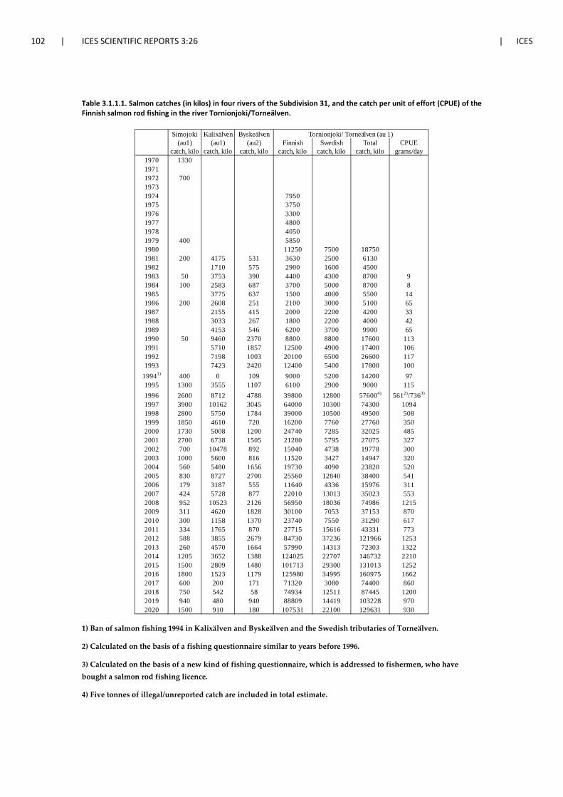
102 | ICES SCIENTIFIC REPORTS 3:26 | ICES
Table 3.1.1.1. Salmon catches (in kilos) in four rivers of the Subdivision 31, and the catch per unit of effort (CPUE) of the Finnish salmon rod fishing in the river Tornionjoki/Torneälven.
1) Ban of salmon fishing 1994 in Kalixälven and Byskeälven and the Swedish tributaries of Torneälven.
2) Calculated on the basis of a fishing questionnaire similar to years before 1996.
3) Calculated on the basis of a new kind of fishing questionnaire, which is addressed to fishermen, who have bought a salmon rod fishing licence.
4) Five tonnes of illegal/unreported catch are included in total estimate.
Simojoki Kalixälven Byskeälven(au1) (au1) (au2) Finnish Swedish Total CPUE
catch, kilo catch, kilo catch, kilo catch, kilo catch, kilo catch, kilo grams/day1970 133019711972 70019731974 79501975 37501976 33001977 48001978 40501979 400 58501980 11250 7500 187501981 200 4175 531 3630 2500 61301982 1710 575 2900 1600 45001983 50 3753 390 4400 4300 8700 91984 100 2583 687 3700 5000 8700 81985 3775 637 1500 4000 5500 141986 200 2608 251 2100 3000 5100 651987 2155 415 2000 2200 4200 331988 3033 267 1800 2200 4000 421989 4153 546 6200 3700 9900 651990 50 9460 2370 8800 8800 17600 1131991 5710 1857 12500 4900 17400 1061992 7198 1003 20100 6500 26600 1171993 7423 2420 12400 5400 17800 100
19941) 400 0 109 9000 5200 14200 971995 1300 3555 1107 6100 2900 9000 1151996 2600 8712 4788 39800 12800 576004) 5612)/7363)
1997 3900 10162 3045 64000 10300 74300 10941998 2800 5750 1784 39000 10500 49500 5081999 1850 4610 720 16200 7760 27760 3502000 1730 5008 1200 24740 7285 32025 4852001 2700 6738 1505 21280 5795 27075 3272002 700 10478 892 15040 4738 19778 3002003 1000 5600 816 11520 3427 14947 3202004 560 5480 1656 19730 4090 23820 5202005 830 8727 2700 25560 12840 38400 5412006 179 3187 555 11640 4336 15976 3112007 424 5728 877 22010 13013 35023 5532008 952 10523 2126 56950 18036 74986 12152009 311 4620 1828 30100 7053 37153 8702010 300 1158 1370 23740 7550 31290 6172011 334 1765 870 27715 15616 43331 7732012 588 3855 2679 84730 37236 121966 12532013 260 4570 1664 57990 14313 72303 13222014 1205 3652 1388 124025 22707 146732 22102015 1500 2809 1480 101713 29300 131013 12522016 1800 1523 1179 125980 34995 160975 16622017 600 200 171 71320 3080 74400 8602018 750 542 58 74934 12511 87445 12002019 940 480 940 88809 14419 103228 9702020 1500 910 180 107531 22100 129631 930
Tornionjoki/ Torneälven (au 1)
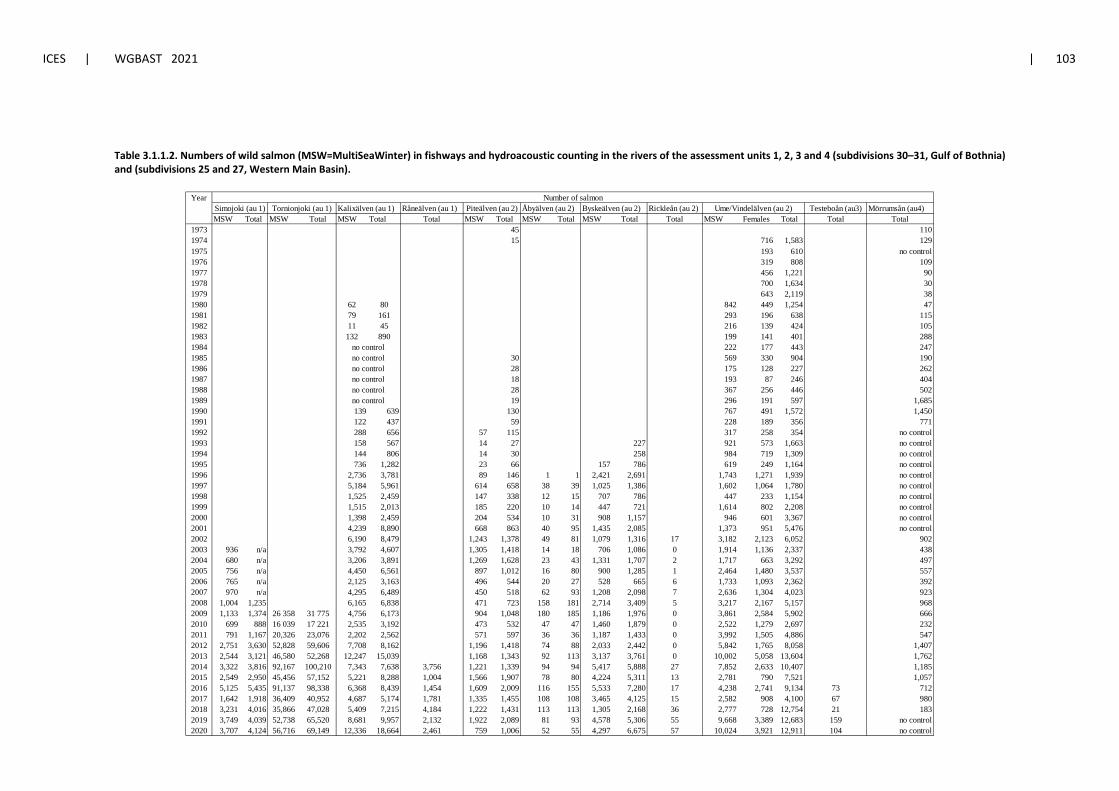
ICES | WGBAST 2021 | 103
Table 3.1.1.2. Numbers of wild salmon (MSW=MultiSeaWinter) in fishways and hydroacoustic counting in the rivers of the assessment units 1, 2, 3 and 4 (subdivisions 30–31, Gulf of Bothnia) and (subdivisions 25 and 27, Western Main Basin).
YearKalixälven (au 1) Råneälven (au 1) Åbyälven (au 2) Byskeälven (au 2) Rickleån (au 2) Testeboån (au3) Mörrumsån (au4)
MSW Total MSW Total MSW Total Total MSW Total MSW Total MSW Total Total MSW Females Total Total Total1973 45 1101974 15 716 1,583 1291975 193 610 no control1976 319 808 1091977 456 1,221 901978 700 1,634 301979 643 2,119 381980 62 80 842 449 1,254 471981 79 161 293 196 638 1151982 11 45 216 139 424 1051983 132 890 199 141 401 2881984 222 177 443 2471985 30 569 330 904 1901986 28 175 128 227 2621987 18 193 87 246 4041988 28 367 256 446 5021989 19 296 191 597 1,6851990 139 639 130 767 491 1,572 1,4501991 122 437 59 228 189 356 7711992 288 656 57 115 317 258 354 no control1993 158 567 14 27 227 921 573 1,663 no control1994 144 806 14 30 258 984 719 1,309 no control1995 736 1,282 23 66 157 786 619 249 1,164 no control1996 2,736 3,781 89 146 1 1 2,421 2,691 1,743 1,271 1,939 no control1997 5,184 5,961 614 658 38 39 1,025 1,386 1,602 1,064 1,780 no control1998 1,525 2,459 147 338 12 15 707 786 447 233 1,154 no control1999 1,515 2,013 185 220 10 14 447 721 1,614 802 2,208 no control2000 1,398 2,459 204 534 10 31 908 1,157 946 601 3,367 no control2001 4,239 8,890 668 863 40 95 1,435 2,085 1,373 951 5,476 no control2002 6,190 8,479 1,243 1,378 49 81 1,079 1,316 17 3,182 2,123 6,052 9022003 936 n/a 3,792 4,607 1,305 1,418 14 18 706 1,086 0 1,914 1,136 2,337 4382004 680 n/a 3,206 3,891 1,269 1,628 23 43 1,331 1,707 2 1,717 663 3,292 4972005 756 n/a 4,450 6,561 897 1,012 16 80 900 1,285 1 2,464 1,480 3,537 5572006 765 n/a 2,125 3,163 496 544 20 27 528 665 6 1,733 1,093 2,362 3922007 970 n/a 4,295 6,489 450 518 62 93 1,208 2,098 7 2,636 1,304 4,023 9232008 1,004 1,235 6,165 6,838 471 723 158 181 2,714 3,409 5 3,217 2,167 5,157 9682009 1,133 1,374 26 358 31 775 4,756 6,173 904 1,048 180 185 1,186 1,976 0 3,861 2,584 5,902 6662010 699 888 16 039 17 221 2,535 3,192 473 532 47 47 1,460 1,879 0 2,522 1,279 2,697 2322011 791 1,167 20,326 23,076 2,202 2,562 571 597 36 36 1,187 1,433 0 3,992 1,505 4,886 5472012 2,751 3,630 52,828 59,606 7,708 8,162 1,196 1,418 74 88 2,033 2,442 0 5,842 1,765 8,058 1,4072013 2,544 3,121 46,580 52,268 12,247 15,039 1,168 1,343 92 113 3,137 3,761 0 10,002 5,058 13,604 1,7622014 3,322 3,816 92,167 100,210 7,343 7,638 3,756 1,221 1,339 94 94 5,417 5,888 27 7,852 2,633 10,407 1,1852015 2,549 2,950 45,456 57,152 5,221 8,288 1,004 1,566 1,907 78 80 4,224 5,311 13 2,781 790 7,521 1,0572016 5,125 5,435 91,137 98,338 6,368 8,439 1,454 1,609 2,009 116 155 5,533 7,280 17 4,238 2,741 9,134 73 7122017 1,642 1,918 36,409 40,952 4,687 5,174 1,781 1,335 1,455 108 108 3,465 4,125 15 2,582 908 4,100 67 9802018 3,231 4,016 35,866 47,028 5,409 7,215 4,184 1,222 1,431 113 113 1,305 2,168 36 2,777 728 12,754 21 1832019 3,749 4,039 52,738 65,520 8,681 9,957 2,132 1,922 2,089 81 93 4,578 5,306 55 9,668 3,389 12,683 159 no control2020 3,707 4,124 56,716 69,149 12,336 18,664 2,461 759 1,006 52 55 4,297 6,675 57 10,024 3,921 12,911 104 no control
Number of salmonSimojoki (au 1) Tornionjoki (au 1) Piteälven (au 2) Ume/Vindelälven (au 2)
no controlno controlno controlno control
no controlno control
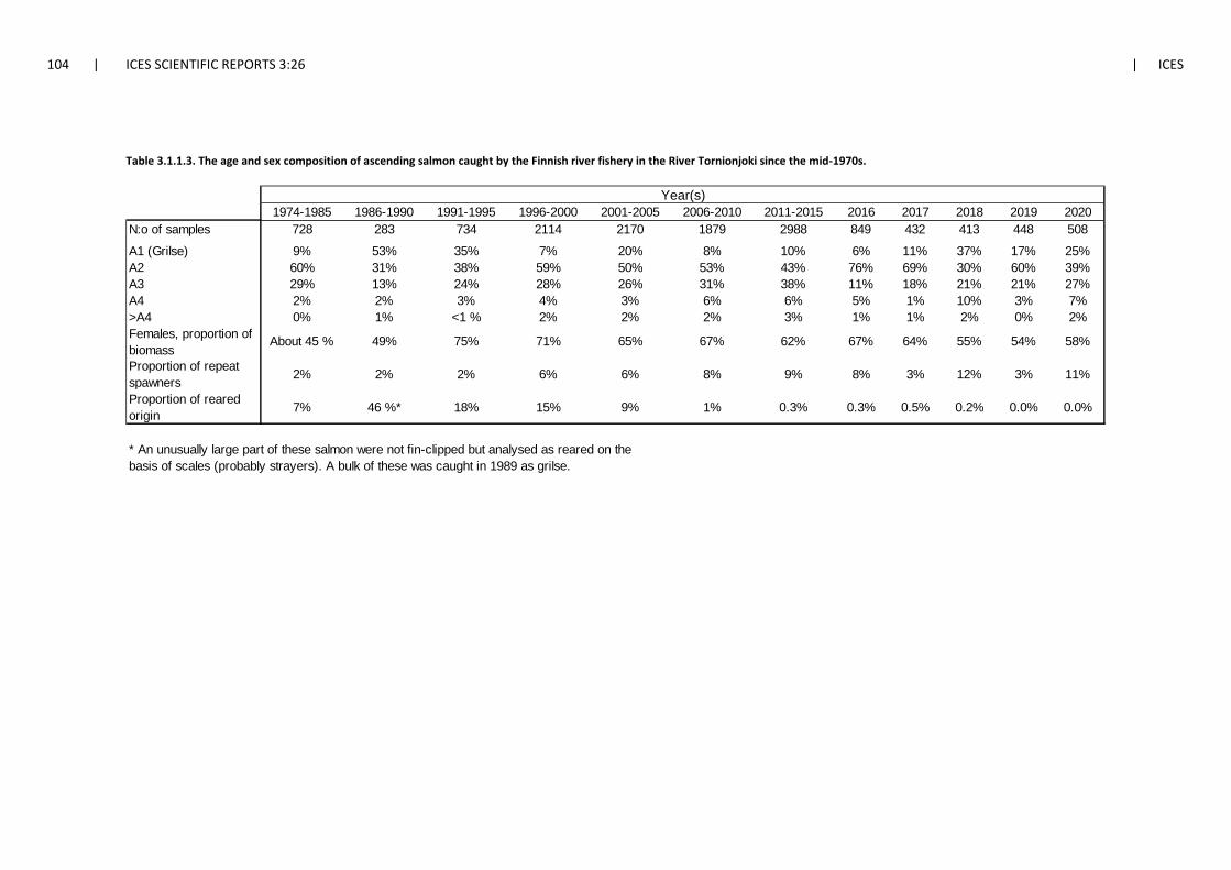
104 | ICES SCIENTIFIC REPORTS 3:26 | ICES
Table 3.1.1.3. The age and sex composition of ascending salmon caught by the Finnish river fishery in the River Tornionjoki since the mid-1970s.
1974-1985 1986-1990 1991-1995 1996-2000 2001-2005 2006-2010 2011-2015 2016 2017 2018 2019 2020N:o of samples 728 283 734 2114 2170 1879 2988 849 432 413 448 508A1 (Grilse) 9% 53% 35% 7% 20% 8% 10% 6% 11% 37% 17% 25%A2 60% 31% 38% 59% 50% 53% 43% 76% 69% 30% 60% 39%A3 29% 13% 24% 28% 26% 31% 38% 11% 18% 21% 21% 27%A4 2% 2% 3% 4% 3% 6% 6% 5% 1% 10% 3% 7%>A4 0% 1% <1 % 2% 2% 2% 3% 1% 1% 2% 0% 2%
* An unusually large part of these salmon were not fin-clipped but analysed as reared on the basis of scales (probably strayers). A bulk of these was caught in 1989 as grilse.
62%
0.3%15% 9%
6% 6% 9%
1%
2% 2%
49% 75% 71% 65%
8%
67%Females, proportion of biomass
Proportion of reared origin 7% 46 %*
About 45 %
18%
Proportion of repeat spawners 2%
0.2%
3%
Year(s)
67%
8%
0.3% 0.0%
54%64%
0.5%
3%
58%
11%
0.0%
55%
12%
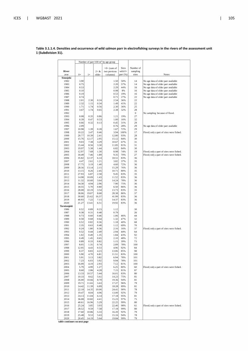
ICES | WGBAST 2021 | 105
Table 3.1.1.4. Densities and occurrence of wild salmon parr in electrofishing surveys in the rivers of the assessment unit 1 (Subdivision 31).
0+ 1+ 2+ & older
>0+ (sum of two previous
columns) Simojoki
1982 3.90 1.50 50% 14 No age data of older parr available1983 0.75 2.20 57% 14 No age data of older parr available1984 0.53 2.29 44% 16 No age data of older parr available1985 0.10 0.98 8% 16 No age data of older parr available1986 0.19 0.53 19% 16 No age data of older parr available1987 0.74 0.71 27% 22 No age data of older parr available1988 2.01 2.30 0.24 2.54 36% 221989 2.32 1.15 0.34 1.49 41% 221990 1.71 1.74 0.56 2.30 36% 251991 3.67 1.74 0.65 2.38 32% 281992 0 No sampling because of flood.1993 0.08 0.35 0.86 1.21 19% 271994 0.39 0.47 0.53 1.00 16% 321995 0.66 0.32 0.13 0.45 31% 291996 2.09 0.76 28% 29 No age data of older parr available1997 10.98 1.39 0.28 1.67 72% 291998 10.22 3.47 0.46 3.94 100% 17 Flood; only a part of sites were fished.1999 20.77 10.39 2.41 12.80 93% 282000 15.76 12.17 2.95 15.12 84% 302001 9.03 7.38 3.29 10.67 67% 312002 15.44 8.56 3.30 11.85 81% 312003 19.97 5.38 1.44 6.82 84% 302004 12.97 7.68 1.30 8.98 74% 19 Flood; only a part of sites were fished.2005 18.49 7.46 1.89 9.35 70% 27 Flood; only a part of sites were fished.2006 35.82 12.37 6.14 18.51 83% 362007 4.47 2.61 1.21 3.82 37% 352008 17.75 3.19 1.40 4.60 72% 362009 28.56 13.14 2.15 15.29 76% 362010 13.15 8.26 2.45 10.71 80% 352011 27.93 6.87 2.58 9.45 83% 352012 14.98 10.09 1.43 11.52 83% 362013 11.32 10.60 3.64 14.24 78% 362014 34.30 4.94 2.96 7.90 75% 362015 18.55 5.70 0.80 6.50 86% 362016 28.08 10.19 3.54 13.73 83% 352017 38.06 19.07 8.68 28.38 86% 372018 30.60 25.62 16.37 41.99 83% 362019 40.93 7.22 7.15 14.37 83% 362020 21.27 13.41 6.51 19.92 83% 36
Tornionjoki1986 0.52 0.89 0.23 1.12 301987 0.38 0.31 0.48 0.79 261988 0.73 0.60 0.46 1.06 46% 441989 0.58 0.68 0.64 1.32 47% 321990 0.52 0.82 0.36 1.18 40% 681991 2.35 0.63 0.48 1.12 69% 701992 0.24 1.80 0.36 2.16 16% 37 Flood; only a part of sites were fished.1993 0.52 0.44 2.49 2.94 44% 641994 1.02 0.49 1.35 1.84 43% 921995 0.49 1.45 0.65 2.10 48% 721996 0.89 0.33 0.82 1.15 39% 731997 8.05 1.35 0.74 2.09 78% 1001998 12.95 4.43 0.53 4.96 92% 841999 8.37 8.83 4.23 13.06 85% 982000 5.90 4.70 6.81 11.51 83% 1002001 5.91 3.13 3.82 6.94 78% 1012002 7.23 6.03 3.92 9.94 78% 1012003 16.09 4.19 2.93 7.12 81% 1002004 5.79 4.99 1.27 6.25 80% 60 Flood; only a part of sites were fished.2005 8.60 2.86 4.28 7.15 81% 872006 13.33 10.57 5.44 16.01 83% 802007 10.33 8.62 5.61 14.23 75% 812008 26.00 10.66 8.70 19.36 94% 812009 19.71 11.65 5.63 17.27 96% 792010 14.42 11.39 6.89 18.28 89% 812011 22.18 14.35 10.06 24.41 90% 782012 19.47 8.04 4.96 13.00 92% 792013 24.13 11.04 6.14 17.18 95% 812014 36.08 10.82 4.41 15.23 97% 752015 40.61 16.96 5.29 22.25 99% 802016 25.24 3.85 3.93 22.46 98% 61 Flood; only a part of sites were fished.2017 28.52 9.59 7.58 17.18 99% 802018 17.60 10.86 5.33 16.20 92% 792019 25.48 9.53 5.63 15.16 94% 782020 20.45 14.19 5.64 19.84 99% 79
table continues on next page
Number of parr/100 m² by age group
Number of sampling
sitesRiver year
Sites with 0+ parr (%) Notes
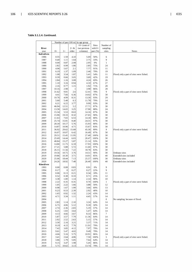
106 | ICES SCIENTIFIC REPORTS 3:26 | ICES
Table 3.1.1.4. Continued.
0+ 1+ 2+ & older
>0+ (sum of two previous
columns) Kalixälven
1986 0.55 1.59 4.10 5.69 50% 61987 0.40 1.11 1.64 2.75 33% 91988 0.00 0.87 2.08 2.95 0% 11989 2.82 0.99 1.86 2.85 75% 241990 4.96 5.67 2.1 7.77 91% 111991 6.19 1.37 1.09 2.46 79% 191992 1.08 3.54 1.87 5.41 54% 11 Flood; only a part of sites were fished.1993 0.59 0.66 3.05 3.69 42% 191994 2.84 1.16 3.08 4.24 69% 261995 1.10 3.16 0.94 4.10 67% 271996 2.16 0.77 1.15 1.92 71% 281997 10.16 2.98 1 3.98 86% 281998 31.62 9.81 2.6 12.41 78% 9 Flood; only a part of sites were fished.1999 4.41 7.66 6.36 14.02 87% 302000 10.76 4.99 8.31 13.30 93% 292001 5.60 5.48 6.3 11.78 79% 142002 6.21 6.22 3.77 9.99 93% 302003 46.94 12.51 5.2 17.71 87% 302004 13.58 14.65 3.25 17.90 88% 242005 15.34 5.53 8.63 14.16 87% 302006 15.96 19.33 8.32 27.65 90% 302007 11.63 7.65 6.53 14.18 80% 302008 25.74 15.91 8.40 24.31 97% 302009 28.18 10.17 5.76 15.93 80% 302010 14.87 10.96 4.71 15.67 83% 302011 36.92 29.62 15.68 45.30 89% 9 Flood; only a part of sites were fished.2012 16.07 10.07 6.42 16.49 87% 302013 29.51 15.45 11.95 27.40 100% 302014 25.69 14.44 6.03 20.47 100% 302015 48.84 15.27 5.87 21.14 93% 302016 14.80 11.75 6.18 17.93 100% 302017 17.21 5.88 5.72 11.60 97% 302018 26.15 11.56 7.22 18.78 83% 302019 19.56 10.75 3.76 14.51 90% 30 Ordinary sites2019 19.86 10.30 3.71 14.01 85% 40 Extended sites included2020 25.06 18.44 7.13 25.57 100% 30 Ordinary sites2020 24.26 18.92 7.48 26.40 100% 40 Extended sites included
Råneälven1993 0.00 0.08 0.83 0.91 0% 91994 0.17 0 0.27 0.27 22% 91995 0.06 0.13 0.21 0.34 18% 111996 0.52 0.38 0.33 0.71 25% 121997 3.38 1.00 1.14 2.14 90% 101998 2.22 0.35 0.35 0.70 100% 1 Flood; only a part of sites were fished.1999 1.05 2.22 1.66 3.88 50% 122000 0.98 1.67 1.99 3.66 69% 132001 0.23 0.53 2.39 2.92 40% 102002 1.65 0.92 1.32 2.24 43% 142003 4.71 3.34 1.11 4.45 57% 142004 0 No sampling because of flood.2005 2.83 1.14 2.10 3.24 64% 142006 6.75 4.06 5.12 9.18 50% 142007 2.74 2.36 2.83 5.19 57% 142008 6.25 1.83 3.64 5.47 64% 142009 4.13 4.66 3.67 8.33 86% 72010 5.87 3.57 7.79 11.36 64% 142011 2.92 2.52 2.63 5.15 57% 142012 3.30 2.16 3.21 5.37 71% 142013 8.19 4.15 7.76 11.91 79% 142014 7.42 3.85 4.12 7.97 79% 142015 9.61 5.47 4.02 9.49 79% 142016 4.66 5.16 5.75 10.91 86% 142017 3.41 2.64 4.86 7.50 100% 5 Flood; only a part of sites were fished.2018 3.86 1.79 5.85 7.64 64% 142019 9.15 3.47 1.98 5.45 86% 142020 5.71 10.62 3.13 13.74 79% 14
NotesRiver year
Number of parr/100 m2 by age groupSites
with 0+ parr (%)
Number of sampling
sites
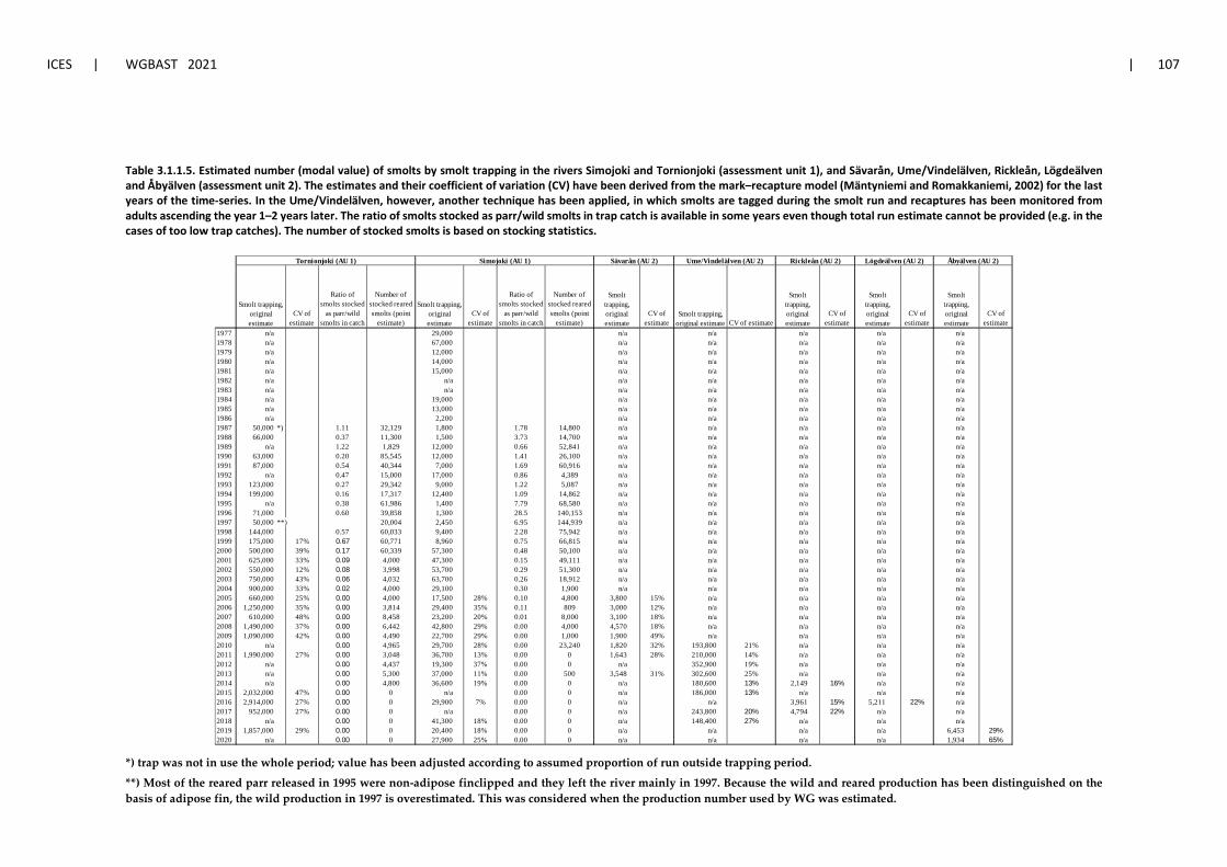
ICES | WGBAST 2021 | 107
Table 3.1.1.5. Estimated number (modal value) of smolts by smolt trapping in the rivers Simojoki and Tornionjoki (assessment unit 1), and Sävarån, Ume/Vindelälven, Rickleån, Lögdeälven and Åbyälven (assessment unit 2). The estimates and their coefficient of variation (CV) have been derived from the mark–recapture model (Mäntyniemi and Romakkaniemi, 2002) for the last years of the time-series. In the Ume/Vindelälven, however, another technique has been applied, in which smolts are tagged during the smolt run and recaptures has been monitored from adults ascending the year 1–2 years later. The ratio of smolts stocked as parr/wild smolts in trap catch is available in some years even though total run estimate cannot be provided (e.g. in the cases of too low trap catches). The number of stocked smolts is based on stocking statistics.
*) trap was not in use the whole period; value has been adjusted according to assumed proportion of run outside trapping period.
**) Most of the reared parr released in 1995 were non-adipose finclipped and they left the river mainly in 1997. Because the wild and reared production has been distinguished on the basis of adipose fin, the wild production in 1997 is overestimated. This was considered when the production number used by WG was estimated.
CV of estimate
Ratio of smolts stocked
as parr/wild smolts in catch
Number of stocked reared smolts (point
estimate)CV of
estimate
Ratio of smolts stocked
as parr/wild smolts in catch
Number of stocked reared smolts (point
estimate)CV of
estimate CV of estimateCV of
estimateCV of
estimateCV of
estimate1977 n/a 29,000 n/a n/a n/a n/a n/a1978 n/a 67,000 n/a n/a n/a n/a n/a1979 n/a 12,000 n/a n/a n/a n/a n/a1980 n/a 14,000 n/a n/a n/a n/a n/a1981 n/a 15,000 n/a n/a n/a n/a n/a1982 n/a n/a n/a n/a n/a n/a n/a1983 n/a n/a n/a n/a n/a n/a n/a1984 n/a 19,000 n/a n/a n/a n/a n/a1985 n/a 13,000 n/a n/a n/a n/a n/a1986 n/a 2,200 n/a n/a n/a n/a n/a1987 50,000 *) 1.11 32,129 1,800 1.78 14,800 n/a n/a n/a n/a n/a1988 66,000 0.37 11,300 1,500 3.73 14,700 n/a n/a n/a n/a n/a1989 n/a 1.22 1,829 12,000 0.66 52,841 n/a n/a n/a n/a n/a1990 63,000 0.20 85,545 12,000 1.41 26,100 n/a n/a n/a n/a n/a1991 87,000 0.54 40,344 7,000 1.69 60,916 n/a n/a n/a n/a n/a1992 n/a 0.47 15,000 17,000 0.86 4,389 n/a n/a n/a n/a n/a1993 123,000 0.27 29,342 9,000 1.22 5,087 n/a n/a n/a n/a n/a1994 199,000 0.16 17,317 12,400 1.09 14,862 n/a n/a n/a n/a n/a1995 n/a 0.38 61,986 1,400 7.79 68,580 n/a n/a n/a n/a n/a1996 71,000 0.60 39,858 1,300 28.5 140,153 n/a n/a n/a n/a n/a1997 50,000 **) 20,004 2,450 6.95 144,939 n/a n/a n/a n/a n/a1998 144,000 0.57 60,033 9,400 2.28 75,942 n/a n/a n/a n/a n/a1999 175,000 17% 0.67 60,771 8,960 0.75 66,815 n/a n/a n/a n/a n/a2000 500,000 39% 0.17 60,339 57,300 0.48 50,100 n/a n/a n/a n/a n/a2001 625,000 33% 0.09 4,000 47,300 0.15 49,111 n/a n/a n/a n/a n/a2002 550,000 12% 0.08 3,998 53,700 0.29 51,300 n/a n/a n/a n/a n/a2003 750,000 43% 0.06 4,032 63,700 0.26 18,912 n/a n/a n/a n/a n/a2004 900,000 33% 0.02 4,000 29,100 0.30 1,900 n/a n/a n/a n/a n/a2005 660,000 25% 0.00 4,000 17,500 28% 0.10 4,800 3,800 15% n/a n/a n/a n/a2006 1,250,000 35% 0.00 3,814 29,400 35% 0.11 809 3,000 12% n/a n/a n/a n/a2007 610,000 48% 0.00 8,458 23,200 20% 0.01 8,000 3,100 18% n/a n/a n/a n/a2008 1,490,000 37% 0.00 6,442 42,800 29% 0.00 4,000 4,570 18% n/a n/a n/a n/a2009 1,090,000 42% 0.00 4,490 22,700 29% 0.00 1,000 1,900 49% n/a n/a n/a n/a2010 n/a 0.00 4,965 29,700 28% 0.00 23,240 1,820 32% 193,800 21% n/a n/a n/a2011 1,990,000 27% 0.00 3,048 36,700 13% 0.00 0 1,643 28% 210,000 14% n/a n/a n/a2012 n/a 0.00 4,437 19,300 37% 0.00 0 n/a 352,900 19% n/a n/a n/a2013 n/a 0.00 5,300 37,000 11% 0.00 500 3,548 31% 302,600 25% n/a n/a n/a2014 n/a 0.00 4,800 36,600 19% 0.00 0 n/a 180,600 13% 2,149 16% n/a n/a2015 2,032,000 47% 0.00 0 n/a 0.00 0 n/a 186,000 13% n/a n/a n/a2016 2,914,000 27% 0.00 0 29,900 7% 0.00 0 n/a n/a 3,961 15% 5,211 22% n/a2017 952,000 27% 0.00 0 n/a 0.00 0 n/a 243,800 20% 4,794 22% n/a n/a2018 n/a 0.00 0 41,300 18% 0.00 0 n/a 148,400 27% n/a n/a n/a2019 1,857,000 29% 0.00 0 20,400 18% 0.00 0 n/a n/a n/a n/a 6,453 29%2020 n/a 0.00 0 27,900 25% 0.00 0 n/a n/a n/a n/a 1,934 65%
Smolt trapping, original estimate
Sävarån (AU 2)
Smolt trapping, original estimate
Simojoki (AU 1)
Smolt trapping, original estimate
Tornionjoki (AU 1) Åbyälven (AU 2)
Smolt trapping, original estimate
Rickleån (AU 2)
Smolt trapping, original estimate
Ume/Vindelälven (AU 2)
Smolt trapping, original estimate
Lögdeälven (AU 2)
Smolt trapping, original estimate
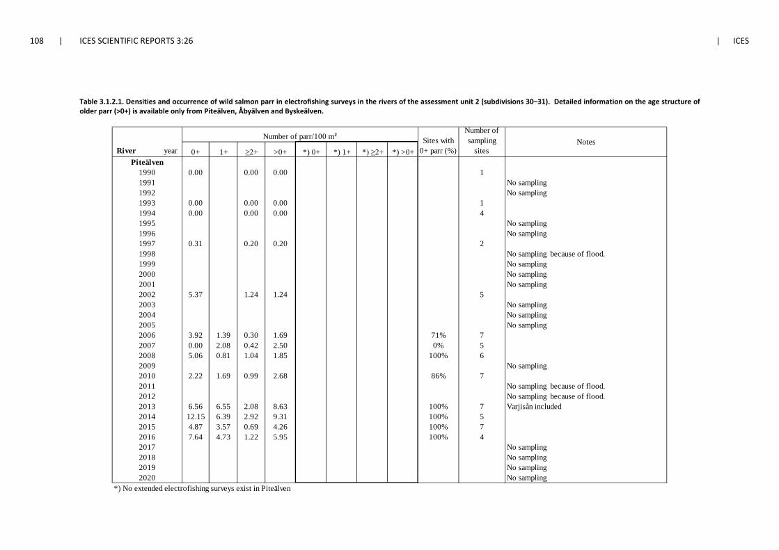
108 | ICES SCIENTIFIC REPORTS 3:26 | ICES
Table 3.1.2.1. Densities and occurrence of wild salmon parr in electrofishing surveys in the rivers of the assessment unit 2 (subdivisions 30–31). Detailed information on the age structure of older parr (>0+) is available only from Piteälven, Åbyälven and Byskeälven.
0+ 1+ ≥2+ >0+ *) 0+ *) 1+ *) ≥2+ *) >0+ Piteälven
1990 0.00 0.00 0.00 11991 No sampling1992 No sampling1993 0.00 0.00 0.00 11994 0.00 0.00 0.00 41995 No sampling1996 No sampling1997 0.31 0.20 0.20 21998 No sampling because of flood.1999 No sampling2000 No sampling2001 No sampling2002 5.37 1.24 1.24 52003 No sampling2004 No sampling2005 No sampling2006 3.92 1.39 0.30 1.69 71% 72007 0.00 2.08 0.42 2.50 0% 52008 5.06 0.81 1.04 1.85 100% 62009 No sampling2010 2.22 1.69 0.99 2.68 86% 72011 No sampling because of flood.2012 No sampling because of flood.2013 6.56 6.55 2.08 8.63 100% 7 Varjisån included2014 12.15 6.39 2.92 9.31 100% 52015 4.87 3.57 0.69 4.26 100% 72016 7.64 4.73 1.22 5.95 100% 42017 No sampling2018 No sampling2019 No sampling2020 No sampling
*) No extended electrofishing surveys exist in Piteälven
Number of sampling
sitesRiver yearSites with
0+ parr (%)Notes
Number of parr/100 m²
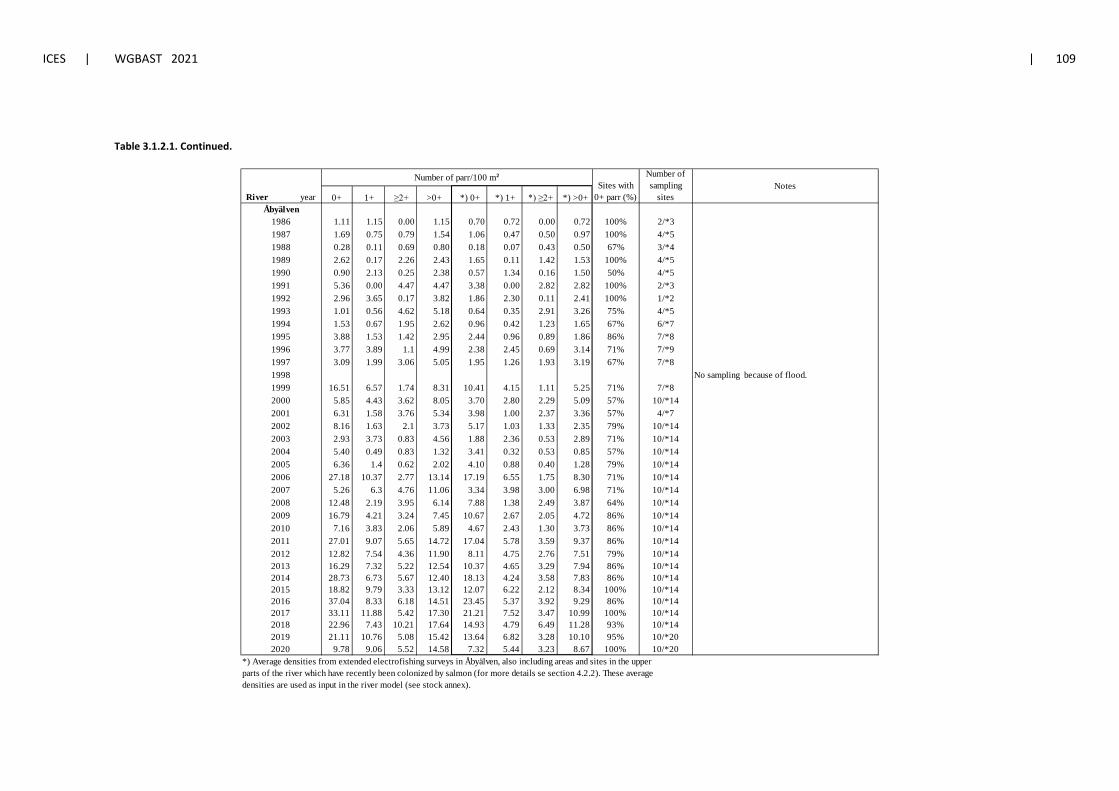
ICES | WGBAST 2021 | 109
Table 3.1.2.1. Continued.
0+ 1+ ≥2+ >0+ *) 0+ *) 1+ *) ≥2+ *) >0+ Åbyälven
1986 1.11 1.15 0.00 1.15 0.70 0.72 0.00 0.72 100% 2/*31987 1.69 0.75 0.79 1.54 1.06 0.47 0.50 0.97 100% 4/*51988 0.28 0.11 0.69 0.80 0.18 0.07 0.43 0.50 67% 3/*41989 2.62 0.17 2.26 2.43 1.65 0.11 1.42 1.53 100% 4/*51990 0.90 2.13 0.25 2.38 0.57 1.34 0.16 1.50 50% 4/*51991 5.36 0.00 4.47 4.47 3.38 0.00 2.82 2.82 100% 2/*31992 2.96 3.65 0.17 3.82 1.86 2.30 0.11 2.41 100% 1/*21993 1.01 0.56 4.62 5.18 0.64 0.35 2.91 3.26 75% 4/*51994 1.53 0.67 1.95 2.62 0.96 0.42 1.23 1.65 67% 6/*71995 3.88 1.53 1.42 2.95 2.44 0.96 0.89 1.86 86% 7/*81996 3.77 3.89 1.1 4.99 2.38 2.45 0.69 3.14 71% 7/*91997 3.09 1.99 3.06 5.05 1.95 1.26 1.93 3.19 67% 7/*81998 No sampling because of flood.1999 16.51 6.57 1.74 8.31 10.41 4.15 1.11 5.25 71% 7/*82000 5.85 4.43 3.62 8.05 3.70 2.80 2.29 5.09 57% 10/*142001 6.31 1.58 3.76 5.34 3.98 1.00 2.37 3.36 57% 4/*72002 8.16 1.63 2.1 3.73 5.17 1.03 1.33 2.35 79% 10/*142003 2.93 3.73 0.83 4.56 1.88 2.36 0.53 2.89 71% 10/*142004 5.40 0.49 0.83 1.32 3.41 0.32 0.53 0.85 57% 10/*142005 6.36 1.4 0.62 2.02 4.10 0.88 0.40 1.28 79% 10/*142006 27.18 10.37 2.77 13.14 17.19 6.55 1.75 8.30 71% 10/*142007 5.26 6.3 4.76 11.06 3.34 3.98 3.00 6.98 71% 10/*142008 12.48 2.19 3.95 6.14 7.88 1.38 2.49 3.87 64% 10/*142009 16.79 4.21 3.24 7.45 10.67 2.67 2.05 4.72 86% 10/*142010 7.16 3.83 2.06 5.89 4.67 2.43 1.30 3.73 86% 10/*142011 27.01 9.07 5.65 14.72 17.04 5.78 3.59 9.37 86% 10/*142012 12.82 7.54 4.36 11.90 8.11 4.75 2.76 7.51 79% 10/*142013 16.29 7.32 5.22 12.54 10.37 4.65 3.29 7.94 86% 10/*142014 28.73 6.73 5.67 12.40 18.13 4.24 3.58 7.83 86% 10/*142015 18.82 9.79 3.33 13.12 12.07 6.22 2.12 8.34 100% 10/*142016 37.04 8.33 6.18 14.51 23.45 5.37 3.92 9.29 86% 10/*142017 33.11 11.88 5.42 17.30 21.21 7.52 3.47 10.99 100% 10/*142018 22.96 7.43 10.21 17.64 14.93 4.79 6.49 11.28 93% 10/*142019 21.11 10.76 5.08 15.42 13.64 6.82 3.28 10.10 95% 10/*202020 9.78 9.06 5.52 14.58 7.32 5.44 3.23 8.67 100% 10/*20
*) Average densities from extended electrofishing surveys in Åbyälven, also including areas and sites in the upper parts of the river which have recently been colonized by salmon (for more details se section 4.2.2). These averagedensities are used as input in the river model (see stock annex).
River yearSites with
0+ parr (%)
Number of sampling
sites
Number of parr/100 m²Notes
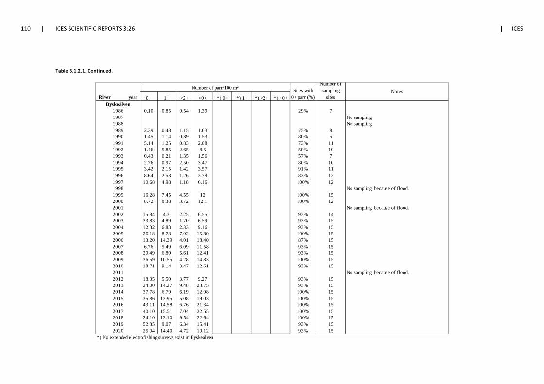
110 | ICES SCIENTIFIC REPORTS 3:26 | ICES
Table 3.1.2.1. Continued.
0+ 1+ ≥2+ >0+ *) 0+ *) 1+ *) ≥2+ *) >0+ Byskeälven
1986 0.10 0.85 0.54 1.39 29% 71987 No sampling1988 No sampling1989 2.39 0.48 1.15 1.63 75% 81990 1.45 1.14 0.39 1.53 80% 51991 5.14 1.25 0.83 2.08 73% 111992 1.46 5.85 2.65 8.5 50% 101993 0.43 0.21 1.35 1.56 57% 71994 2.76 0.97 2.50 3.47 80% 101995 3.42 2.15 1.42 3.57 91% 111996 8.64 2.53 1.26 3.79 83% 121997 10.68 4.98 1.18 6.16 100% 121998 No sampling because of flood.1999 16.28 7.45 4.55 12 100% 152000 8.72 8.38 3.72 12.1 100% 122001 No sampling because of flood.2002 15.84 4.3 2.25 6.55 93% 142003 33.83 4.89 1.70 6.59 93% 152004 12.32 6.83 2.33 9.16 93% 152005 26.18 8.78 7.02 15.80 100% 152006 13.20 14.39 4.01 18.40 87% 152007 6.76 5.49 6.09 11.58 93% 152008 20.49 6.80 5.61 12.41 93% 152009 36.59 10.55 4.28 14.83 100% 152010 18.71 9.14 3.47 12.61 93% 152011 No sampling because of flood.2012 18.35 5.50 3.77 9.27 93% 152013 24.00 14.27 9.48 23.75 93% 152014 37.78 6.79 6.19 12.98 100% 152015 35.86 13.95 5.08 19.03 100% 152016 43.11 14.58 6.76 21.34 100% 152017 40.10 15.51 7.04 22.55 100% 152018 24.10 13.10 9.54 22.64 100% 152019 52.35 9.07 6.34 15.41 93% 152020 25.04 14.40 4.72 19.12 93% 15
*) No extended electrofishing surveys exist in Byskeälven
Sites with 0+ parr (%)River year
Number of sampling
sites
Number of parr/100 m²Notes
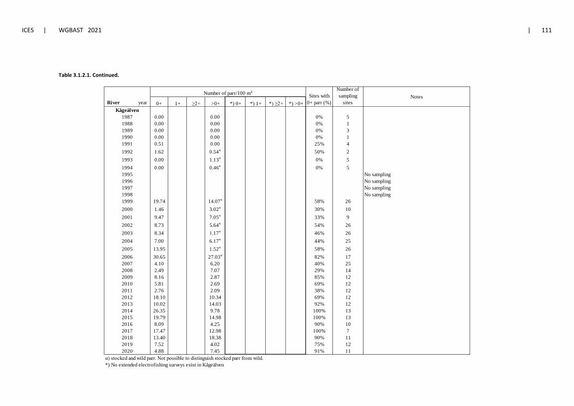
ICES | WGBAST 2021 | 111
Table 3.1.2.1. Continued.
0+ 1+ ≥2+ >0+ *) 0+ *) 1+ *) ≥2+ *) >0+ Kågeälven
1987 0.00 0.00 0% 51988 0.00 0.00 0% 11989 0.00 0.00 0% 31990 0.00 0.00 0% 11991 0.51 0.00 25% 41992 1.62 0.54α 50% 21993 0.00 1.13α 0% 51994 0.00 0.46α 0% 51995 No sampling1996 No sampling1997 No sampling1998 No sampling1999 19.74 14.07α 58% 262000 1.46 3.02α 30% 102001 9.47 7.05α 33% 92002 8.73 5.64α 54% 262003 8.34 1.17α 46% 262004 7.00 6.17α 44% 252005 13.95 1.52α 58% 262006 30.65 27.03α 82% 172007 4.10 6.20 40% 252008 2.49 7.07 29% 142009 8.16 2.87 85% 122010 5.81 2.69 69% 122011 2.76 2.09 38% 122012 18.10 10.34 69% 122013 10.02 14.03 92% 122014 26.35 9.78 100% 132015 19.79 14.98 100% 132016 8.09 4.25 90% 102017 17.47 12.98 100% 72018 13.40 18.38 90% 112019 7.52 4.02 75% 122020 4.88 7.45 91% 11
α) stocked and wild parr. Not possible to distinguish stocked parr from wild.*) No extended electrofishing surveys exist in Kågeälven
River yearSites with
0+ parr (%)
Number of sampling
sitesNotes
Number of parr/100 m²
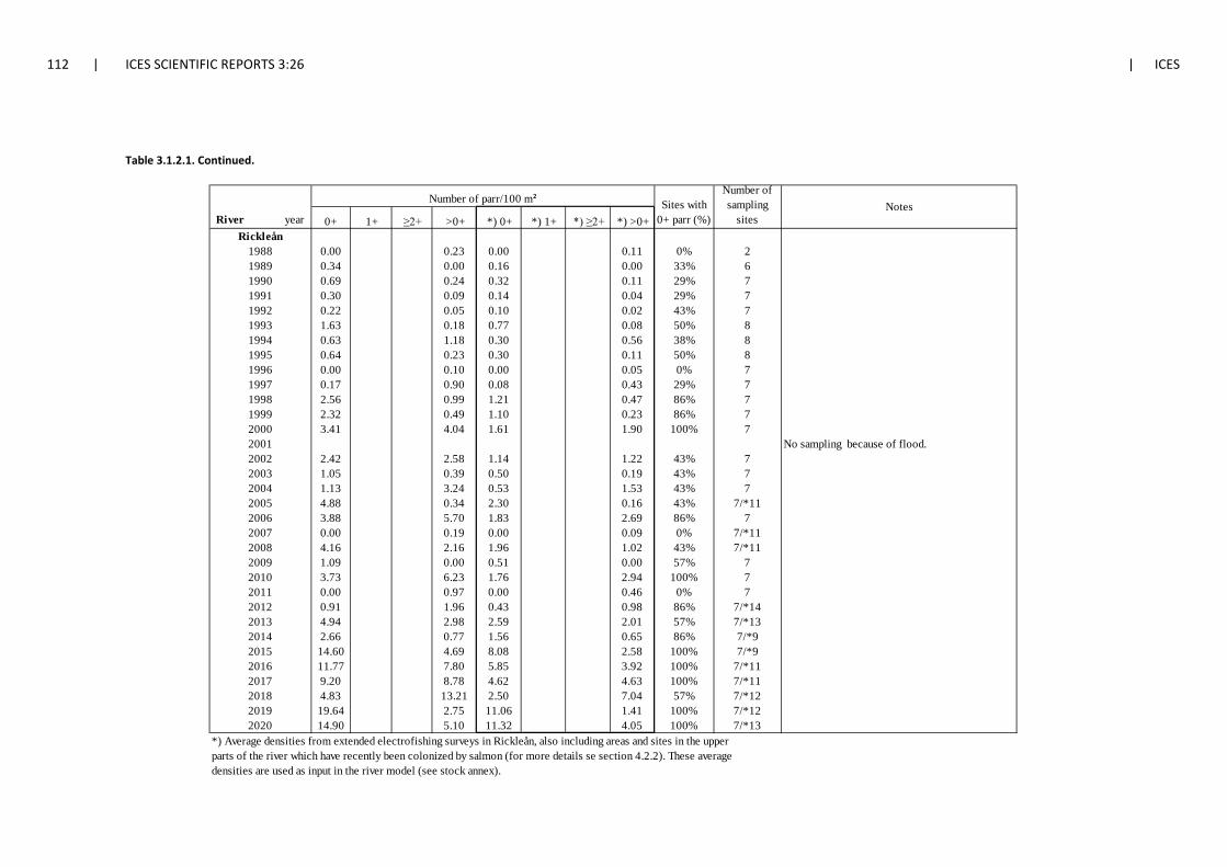
112 | ICES SCIENTIFIC REPORTS 3:26 | ICES
Table 3.1.2.1. Continued.
0+ 1+ ≥2+ >0+ *) 0+ *) 1+ *) ≥2+ *) >0+ Rickleån
1988 0.00 0.23 0.00 0.11 0% 21989 0.34 0.00 0.16 0.00 33% 61990 0.69 0.24 0.32 0.11 29% 71991 0.30 0.09 0.14 0.04 29% 71992 0.22 0.05 0.10 0.02 43% 71993 1.63 0.18 0.77 0.08 50% 81994 0.63 1.18 0.30 0.56 38% 81995 0.64 0.23 0.30 0.11 50% 81996 0.00 0.10 0.00 0.05 0% 71997 0.17 0.90 0.08 0.43 29% 71998 2.56 0.99 1.21 0.47 86% 71999 2.32 0.49 1.10 0.23 86% 72000 3.41 4.04 1.61 1.90 100% 72001 No sampling because of flood.2002 2.42 2.58 1.14 1.22 43% 72003 1.05 0.39 0.50 0.19 43% 72004 1.13 3.24 0.53 1.53 43% 72005 4.88 0.34 2.30 0.16 43% 7/*112006 3.88 5.70 1.83 2.69 86% 72007 0.00 0.19 0.00 0.09 0% 7/*112008 4.16 2.16 1.96 1.02 43% 7/*112009 1.09 0.00 0.51 0.00 57% 72010 3.73 6.23 1.76 2.94 100% 72011 0.00 0.97 0.00 0.46 0% 72012 0.91 1.96 0.43 0.98 86% 7/*142013 4.94 2.98 2.59 2.01 57% 7/*132014 2.66 0.77 1.56 0.65 86% 7/*92015 14.60 4.69 8.08 2.58 100% 7/*92016 11.77 7.80 5.85 3.92 100% 7/*112017 9.20 8.78 4.62 4.63 100% 7/*112018 4.83 13.21 2.50 7.04 57% 7/*122019 19.64 2.75 11.06 1.41 100% 7/*122020 14.90 5.10 11.32 4.05 100% 7/*13
*) Average densities from extended electrofishing surveys in Rickleån, also including areas and sites in the upper parts of the river which have recently been colonized by salmon (for more details se section 4.2.2). These averagedensities are used as input in the river model (see stock annex).
River yearSites with
0+ parr (%)
Number of sampling
sitesNotes
Number of parr/100 m²
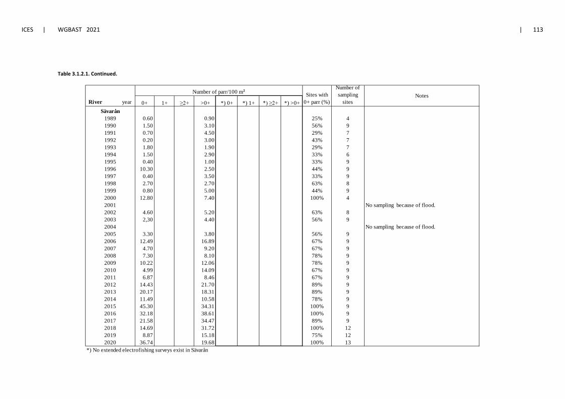
ICES | WGBAST 2021 | 113
Table 3.1.2.1. Continued.
0+ 1+ ≥2+ >0+ *) 0+ *) 1+ *) ≥2+ *) >0+ Sävarån
1989 0.60 0.90 25% 41990 1.50 3.10 56% 91991 0.70 4.50 29% 71992 0.20 3.00 43% 71993 1.80 1.90 29% 71994 1.50 2.90 33% 61995 0.40 1.00 33% 91996 10.30 2.50 44% 91997 0.40 3.50 33% 91998 2.70 2.70 63% 81999 0.80 5.00 44% 92000 12.80 7.40 100% 42001 No sampling because of flood.2002 4.60 5.20 63% 82003 2,30 4.40 56% 92004 No sampling because of flood.2005 3.30 3.80 56% 92006 12.49 16.89 67% 92007 4.70 9.20 67% 92008 7.30 8.10 78% 92009 10.22 12.06 78% 92010 4.99 14.09 67% 92011 6.87 8.46 67% 92012 14.43 21.70 89% 92013 20.17 18.31 89% 92014 11.49 10.58 78% 92015 45.30 34.31 100% 92016 32.18 38.61 100% 92017 21.58 34.47 89% 92018 14.69 31.72 100% 122019 8.87 15.18 75% 122020 36.74 19.68 100% 13
*) No extended electrofishing surveys exist in Sävarån
Sites with 0+ parr (%)
Number of sampling
sitesRiver yearNotes
Number of parr/100 m²
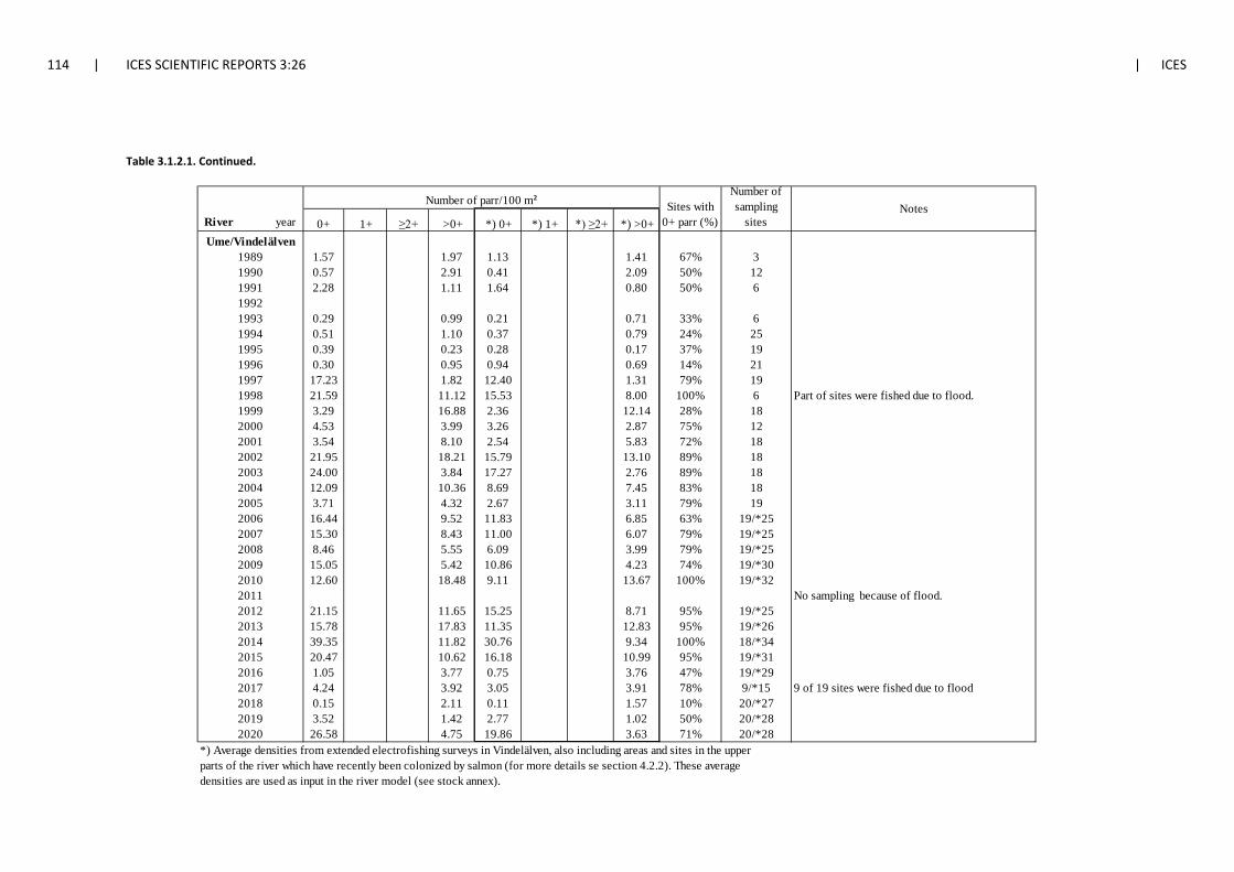
114 | ICES SCIENTIFIC REPORTS 3:26 | ICES
Table 3.1.2.1. Continued.
0+ 1+ ≥2+ >0+ *) 0+ *) 1+ *) ≥2+ *) >0+ Ume/Vindelälven
1989 1.57 1.97 1.13 1.41 67% 31990 0.57 2.91 0.41 2.09 50% 121991 2.28 1.11 1.64 0.80 50% 619921993 0.29 0.99 0.21 0.71 33% 61994 0.51 1.10 0.37 0.79 24% 251995 0.39 0.23 0.28 0.17 37% 191996 0.30 0.95 0.94 0.69 14% 211997 17.23 1.82 12.40 1.31 79% 191998 21.59 11.12 15.53 8.00 100% 6 Part of sites were fished due to flood.1999 3.29 16.88 2.36 12.14 28% 182000 4.53 3.99 3.26 2.87 75% 122001 3.54 8.10 2.54 5.83 72% 182002 21.95 18.21 15.79 13.10 89% 182003 24.00 3.84 17.27 2.76 89% 182004 12.09 10.36 8.69 7.45 83% 182005 3.71 4.32 2.67 3.11 79% 192006 16.44 9.52 11.83 6.85 63% 19/*252007 15.30 8.43 11.00 6.07 79% 19/*252008 8.46 5.55 6.09 3.99 79% 19/*252009 15.05 5.42 10.86 4.23 74% 19/*302010 12.60 18.48 9.11 13.67 100% 19/*322011 No sampling because of flood.2012 21.15 11.65 15.25 8.71 95% 19/*252013 15.78 17.83 11.35 12.83 95% 19/*262014 39.35 11.82 30.76 9.34 100% 18/*342015 20.47 10.62 16.18 10.99 95% 19/*312016 1.05 3.77 0.75 3.76 47% 19/*292017 4.24 3.92 3.05 3.91 78% 9/*15 9 of 19 sites were fished due to flood2018 0.15 2.11 0.11 1.57 10% 20/*272019 3.52 1.42 2.77 1.02 50% 20/*282020 26.58 4.75 19.86 3.63 71% 20/*28
*) Average densities from extended electrofishing surveys in Vindelälven, also including areas and sites in the upper parts of the river which have recently been colonized by salmon (for more details se section 4.2.2). These averagedensities are used as input in the river model (see stock annex).
River yearSites with
0+ parr (%)
Number of sampling
sitesNotes
Number of parr/100 m²
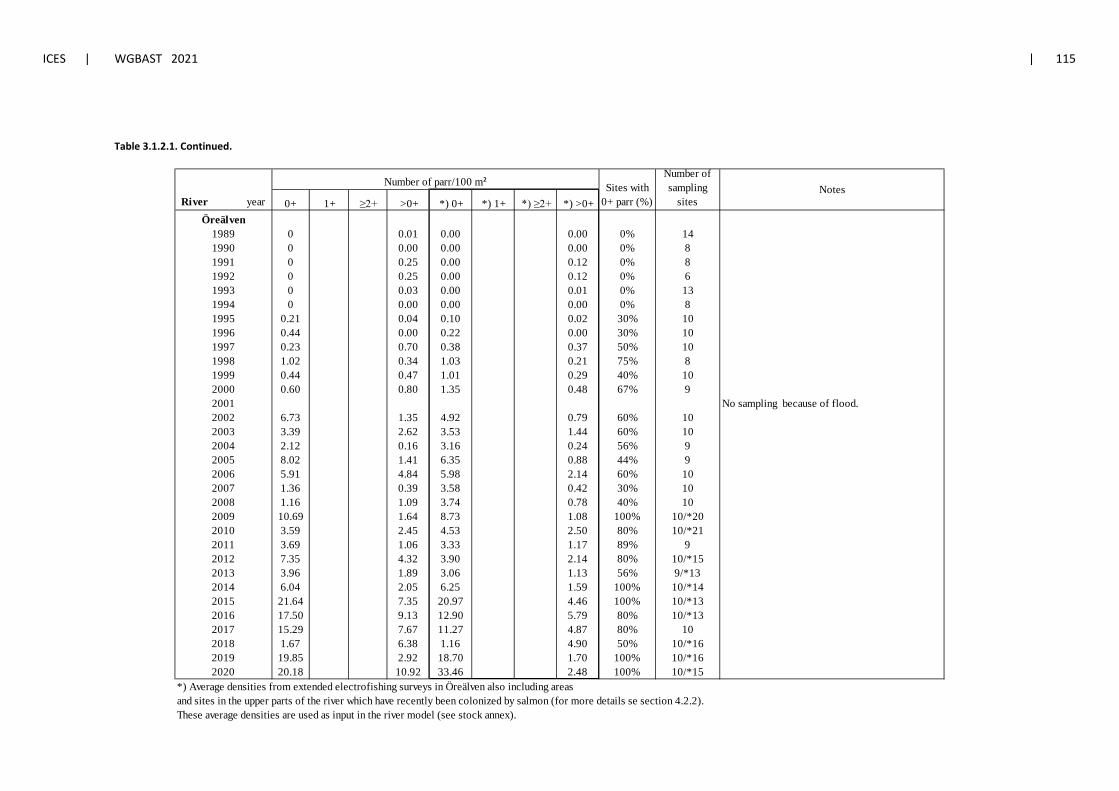
ICES | WGBAST 2021 | 115
Table 3.1.2.1. Continued.
0+ 1+ ≥2+ >0+ *) 0+ *) 1+ *) ≥2+ *) >0+ Öreälven
1989 0 0.01 0.00 0.00 0% 141990 0 0.00 0.00 0.00 0% 81991 0 0.25 0.00 0.12 0% 81992 0 0.25 0.00 0.12 0% 61993 0 0.03 0.00 0.01 0% 131994 0 0.00 0.00 0.00 0% 81995 0.21 0.04 0.10 0.02 30% 101996 0.44 0.00 0.22 0.00 30% 101997 0.23 0.70 0.38 0.37 50% 101998 1.02 0.34 1.03 0.21 75% 81999 0.44 0.47 1.01 0.29 40% 102000 0.60 0.80 1.35 0.48 67% 92001 No sampling because of flood.2002 6.73 1.35 4.92 0.79 60% 102003 3.39 2.62 3.53 1.44 60% 102004 2.12 0.16 3.16 0.24 56% 92005 8.02 1.41 6.35 0.88 44% 92006 5.91 4.84 5.98 2.14 60% 102007 1.36 0.39 3.58 0.42 30% 102008 1.16 1.09 3.74 0.78 40% 102009 10.69 1.64 8.73 1.08 100% 10/*202010 3.59 2.45 4.53 2.50 80% 10/*212011 3.69 1.06 3.33 1.17 89% 92012 7.35 4.32 3.90 2.14 80% 10/*152013 3.96 1.89 3.06 1.13 56% 9/*132014 6.04 2.05 6.25 1.59 100% 10/*142015 21.64 7.35 20.97 4.46 100% 10/*132016 17.50 9.13 12.90 5.79 80% 10/*132017 15.29 7.67 11.27 4.87 80% 102018 1.67 6.38 1.16 4.90 50% 10/*162019 19.85 2.92 18.70 1.70 100% 10/*162020 20.18 10.92 33.46 2.48 100% 10/*15
*) Average densities from extended electrofishing surveys in Öreälven also including areasand sites in the upper parts of the river which have recently been colonized by salmon (for more details se section 4.2.2).These average densities are used as input in the river model (see stock annex).
Number of sampling
sitesRiver yearNotes
Number of parr/100 m² Sites with 0+ parr (%)
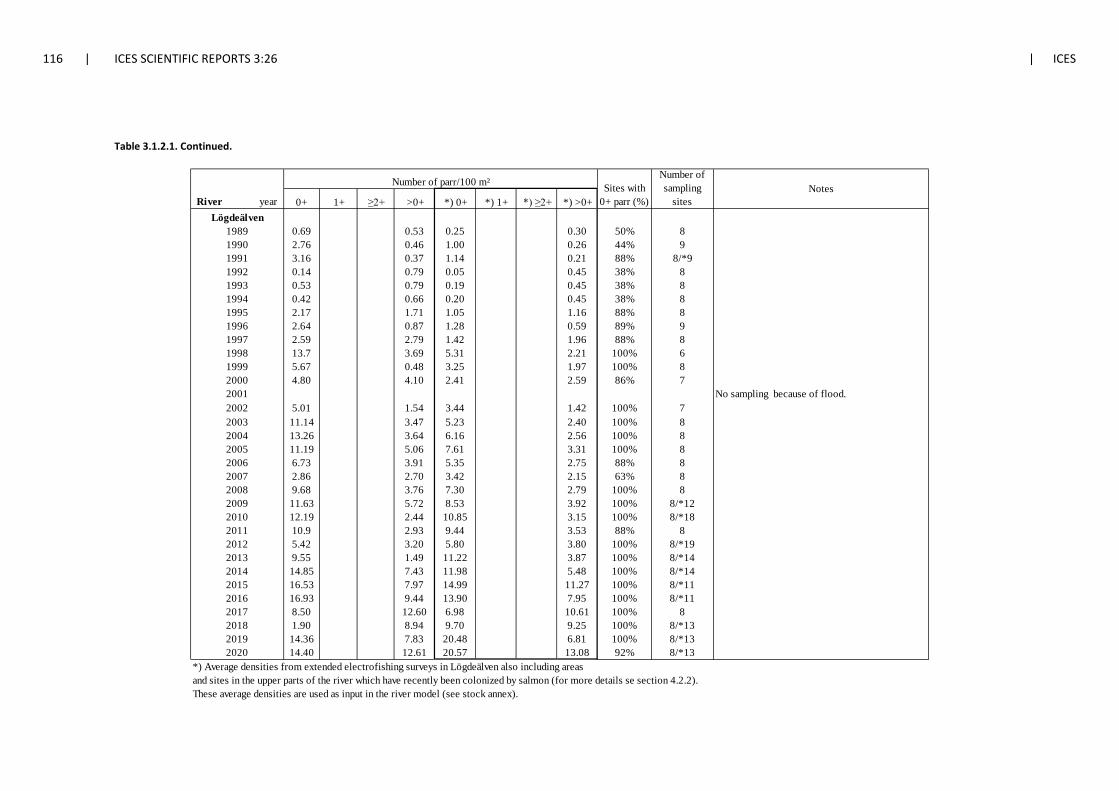
116 | ICES SCIENTIFIC REPORTS 3:26 | ICES
Table 3.1.2.1. Continued.
0+ 1+ ≥2+ >0+ *) 0+ *) 1+ *) ≥2+ *) >0+ Lögdeälven
1989 0.69 0.53 0.25 0.30 50% 81990 2.76 0.46 1.00 0.26 44% 91991 3.16 0.37 1.14 0.21 88% 8/*91992 0.14 0.79 0.05 0.45 38% 81993 0.53 0.79 0.19 0.45 38% 81994 0.42 0.66 0.20 0.45 38% 81995 2.17 1.71 1.05 1.16 88% 81996 2.64 0.87 1.28 0.59 89% 91997 2.59 2.79 1.42 1.96 88% 81998 13.7 3.69 5.31 2.21 100% 61999 5.67 0.48 3.25 1.97 100% 82000 4.80 4.10 2.41 2.59 86% 72001 No sampling because of flood.2002 5.01 1.54 3.44 1.42 100% 72003 11.14 3.47 5.23 2.40 100% 82004 13.26 3.64 6.16 2.56 100% 82005 11.19 5.06 7.61 3.31 100% 82006 6.73 3.91 5.35 2.75 88% 82007 2.86 2.70 3.42 2.15 63% 82008 9.68 3.76 7.30 2.79 100% 82009 11.63 5.72 8.53 3.92 100% 8/*122010 12.19 2.44 10.85 3.15 100% 8/*182011 10.9 2.93 9.44 3.53 88% 82012 5.42 3.20 5.80 3.80 100% 8/*192013 9.55 1.49 11.22 3.87 100% 8/*142014 14.85 7.43 11.98 5.48 100% 8/*142015 16.53 7.97 14.99 11.27 100% 8/*112016 16.93 9.44 13.90 7.95 100% 8/*112017 8.50 12.60 6.98 10.61 100% 82018 1.90 8.94 9.70 9.25 100% 8/*132019 14.36 7.83 20.48 6.81 100% 8/*132020 14.40 12.61 20.57 13.08 92% 8/*13
*) Average densities from extended electrofishing surveys in Lögdeälven also including areasand sites in the upper parts of the river which have recently been colonized by salmon (for more details se section 4.2.2).These average densities are used as input in the river model (see stock annex).
River yearSites with
0+ parr (%)
Number of sampling
sitesNotesNumber of parr/100 m²
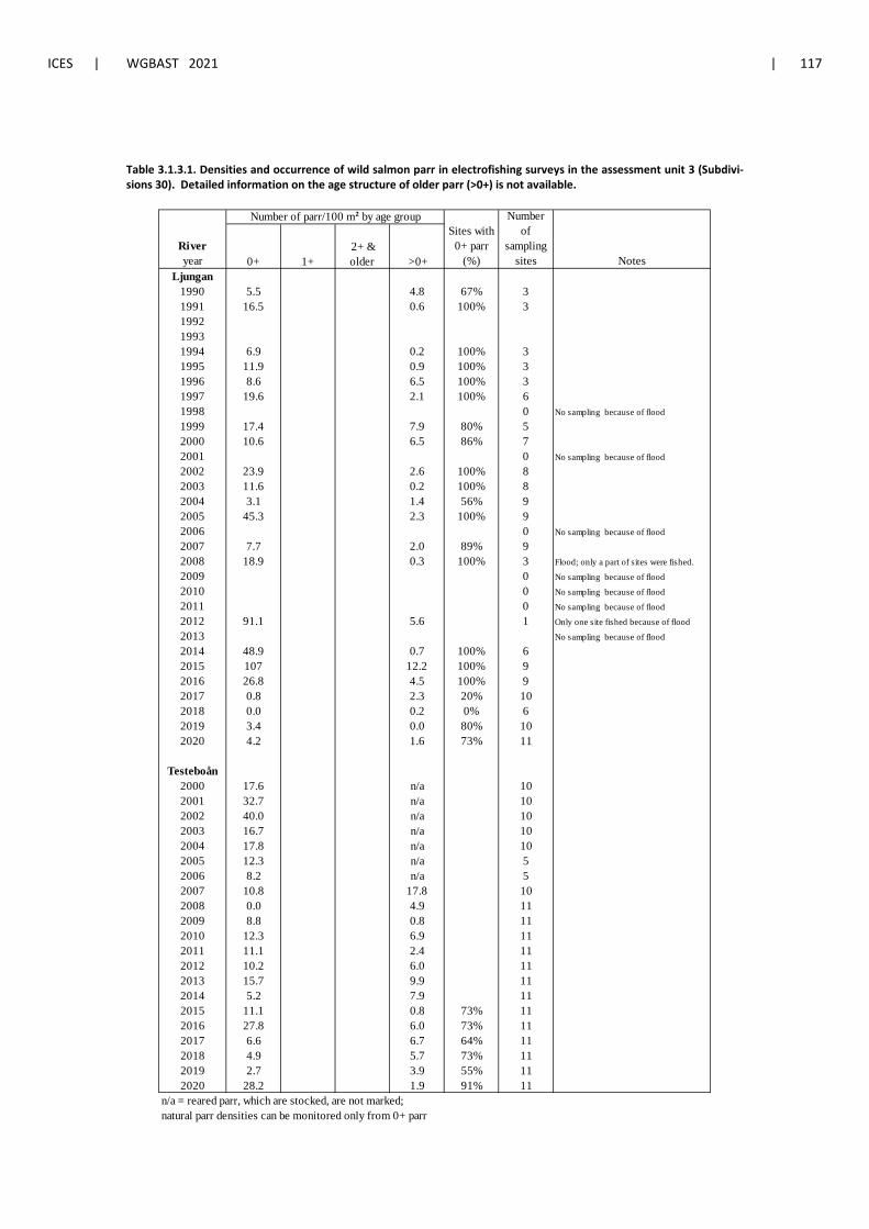
ICES | WGBAST 2021 | 117
Table 3.1.3.1. Densities and occurrence of wild salmon parr in electrofishing surveys in the assessment unit 3 (Subdivi-sions 30). Detailed information on the age structure of older parr (>0+) is not available.
0+ 1+ 2+ & older >0+
Ljungan1990 5.5 4.8 67% 31991 16.5 0.6 100% 3199219931994 6.9 0.2 100% 31995 11.9 0.9 100% 31996 8.6 6.5 100% 31997 19.6 2.1 100% 61998 0 No sampling because of flood
1999 17.4 7.9 80% 52000 10.6 6.5 86% 72001 0 No sampling because of flood
2002 23.9 2.6 100% 82003 11.6 0.2 100% 82004 3.1 1.4 56% 92005 45.3 2.3 100% 92006 0 No sampling because of flood
2007 7.7 2.0 89% 92008 18.9 0.3 100% 3 Flood; only a part of sites were fished.
2009 0 No sampling because of flood
2010 0 No sampling because of flood
2011 0 No sampling because of flood
2012 91.1 5.6 1 Only one site fished because of flood
2013 No sampling because of flood
2014 48.9 0.7 100% 62015 107 12.2 100% 92016 26.8 4.5 100% 92017 0.8 2.3 20% 102018 0.0 0.2 0% 62019 3.4 0.0 80% 102020 4.2 1.6 73% 11
Testeboån2000 17.6 n/a 102001 32.7 n/a 102002 40.0 n/a 102003 16.7 n/a 102004 17.8 n/a 102005 12.3 n/a 52006 8.2 n/a 52007 10.8 17.8 102008 0.0 4.9 112009 8.8 0.8 112010 12.3 6.9 112011 11.1 2.4 112012 10.2 6.0 112013 15.7 9.9 112014 5.2 7.9 112015 11.1 0.8 73% 112016 27.8 6.0 73% 112017 6.6 6.7 64% 112018 4.9 5.7 73% 112019 2.7 3.9 55% 112020 28.2 1.9 91% 11
n/a = reared parr, which are stocked, are not marked; natural parr densities can be monitored only from 0+ parr
River year
Number of parr/100 m² by age groupSites with
0+ parr (%)
Number of
sampling sites Notes
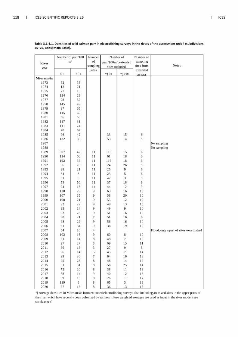
118 | ICES SCIENTIFIC REPORTS 3:26 | ICES
Table 3.1.4.1. Densities of wild salmon parr in electrofishing surveys in the rivers of the assessment unit 4 (subdivisions 25–26, Baltic Main Basin).
0+ >0+ *) 0+ *) >0+Mörrumsån
1973 32 331974 12 211975 77 131976 124 291977 78 571978 145 491979 97 651980 115 601981 56 501982 117 311983 111 741984 70 671985 96 42 33 15 61986 132 39 53 14 51987 No sampling1988 No sampling1989 307 42 11 116 15 61990 114 60 11 61 18 61991 192 55 11 116 18 51992 36 78 11 24 26 51993 28 21 11 25 9 61994 34 8 11 23 5 61995 61 5 11 47 3 91996 53 50 11 37 18 91997 74 15 14 44 12 91998 120 29 9 63 16 101999 107 35 9 58 20 102000 108 21 9 55 12 102001 92 22 9 49 13 102002 95 14 9 49 9 102003 92 28 9 51 16 102004 80 21 7 51 16 62005 98 29 9 56 16 102006 61 34 9 36 19 102007 54 10 4 Flood, only a part of sites were fished.2008 102 16 9 60 8 102009 61 14 8 48 7 102010 97 27 8 69 15 112011 36 18 5 27 9 82012 96 14 5 45 7 142013 99 30 7 64 16 182014 95 23 8 48 14 172015 81 31 8 56 25 142016 72 20 8 38 11 182017 58 14 9 40 12 182018 39 15 8 26 11 172019 119 6 8 65 3 182020 37 13 8 36 13 18
Number of parr/100 m²
Number of parr/100m², extended
sites included. Notes
*) Average densities in Mörrumsån from extended electrofishing surveys also including areas and sites in the upper parts of the river which have recently been colonized by salmon. These weighted averages are used as input in the river model (see stock annex)
River year
Number of sampling
sites from extended survays
Number of
sampling sites
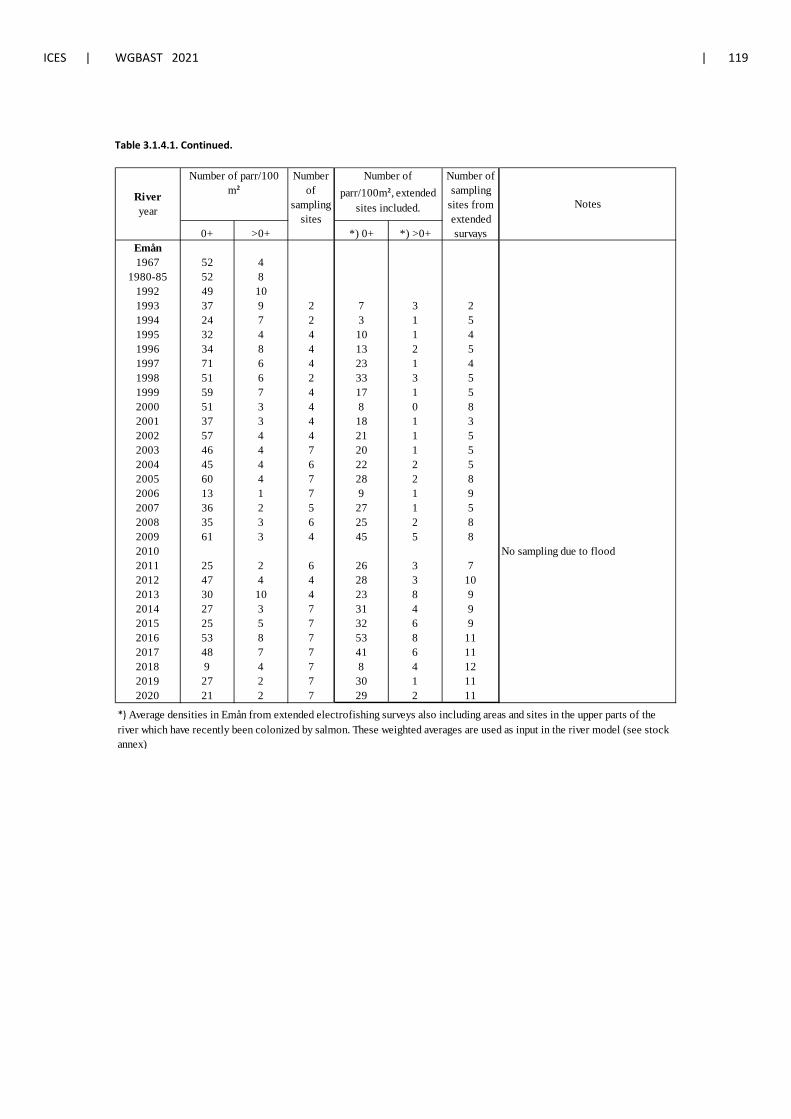
ICES | WGBAST 2021 | 119
Table 3.1.4.1. Continued.
0+ >0+ *) 0+ *) >0+Emån1967 52 4
1980-85 52 81992 49 101993 37 9 2 7 3 21994 24 7 2 3 1 51995 32 4 4 10 1 41996 34 8 4 13 2 51997 71 6 4 23 1 41998 51 6 2 33 3 51999 59 7 4 17 1 52000 51 3 4 8 0 82001 37 3 4 18 1 32002 57 4 4 21 1 52003 46 4 7 20 1 52004 45 4 6 22 2 52005 60 4 7 28 2 82006 13 1 7 9 1 92007 36 2 5 27 1 52008 35 3 6 25 2 82009 61 3 4 45 5 82010 No sampling due to flood2011 25 2 6 26 3 72012 47 4 4 28 3 102013 30 10 4 23 8 92014 27 3 7 31 4 92015 25 5 7 32 6 92016 53 8 7 53 8 112017 48 7 7 41 6 112018 9 4 7 8 4 122019 27 2 7 30 1 112020 21 2 7 29 2 11
*) Average densities in Emån from extended electrofishing surveys also including areas and sites in the upper parts of the river which have recently been colonized by salmon. These weighted averages are used as input in the river model (see stock annex)
Number of parr/100 m²
Number of
sampling sites
Number of parr/100m², extended
sites included.
Number of sampling
sites from extended survays
NotesRiver year
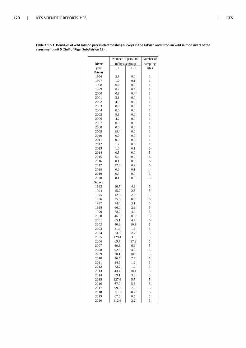
120 | ICES SCIENTIFIC REPORTS 3:26 | ICES
Table 3.1.5.1. Densities of wild salmon parr in electrofishing surveys in the Latvian and Estonian wild salmon rivers of the assessment unit 5 (Gulf of Riga. Subdivision 28).
Number ofsampling
0+ >0+ sitesPärnu1996 3.8 0.0 11997 1.0 0.1 11998 0.0 0.0 11999 0.2 0.4 12000 0.8 0.4 12001 3.1 0.0 12002 4.9 0.0 12003 0.0 0.0 12004 0.0 0.0 12005 9.8 0.0 12006 4.2 0.0 12007 0.0 0.0 12008 0.0 0.0 12009 18.4 0.0 12010 0.0 0.0 12011 0.0 0.0 12012 1.7 0.0 12013 1.0 0.1 52014 0.5 0.0 52015 5.4 0.2 62016 0.1 0.3 62017 22.8 0.2 52018 0.6 0.1 142019 6.5 0.0 52020 8.1 0.0 5
Salaca1993 16.7 4.9 51994 15.2 2.6 51995 12.8 2.8 51996 25.3 0.9 61997 74.4 3.1 51998 60.0 2.8 51999 68.7 4.0 52000 46.3 0.8 52001 65.1 4.4 52002 40.2 10.3 62003 31.5 1.3 52004 73.8 2.7 52005 129.4 3.8 52006 69.7 17.9 52007 69.6 6.9 52008 92.3 4.9 52009 70.1 10.3 52010 26.5 7.4 52011 34.5 1.2 52012 72.2 1.9 52013 43.4 10.4 52014 59.1 3.8 52015 137.6 5.7 52016 67.7 5.5 52017 99.9 7.3 52018 21.3 8.2 52019 67.6 0.5 52020 112.6 2.2 5
River year
Number of parr/100 m2 by age group
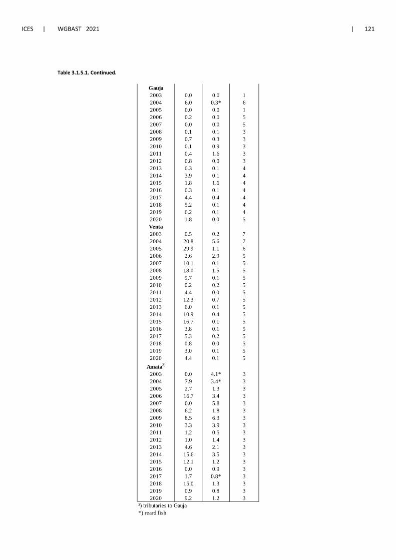
ICES | WGBAST 2021 | 121
Table 3.1.5.1. Continued.
Gauja2003 0.0 0.0 12004 6.0 0.3* 62005 0.0 0.0 12006 0.2 0.0 52007 0.0 0.0 52008 0.1 0.1 32009 0.7 0.3 32010 0.1 0.9 32011 0.4 1.6 32012 0.8 0.0 32013 0.3 0.1 42014 3.9 0.1 42015 1.8 1.6 42016 0.3 0.1 42017 4.4 0.4 42018 5.2 0.1 42019 6.2 0.1 42020 1.8 0.0 5Venta2003 0.5 0.2 72004 20.8 5.6 72005 29.9 1.1 62006 2.6 2.9 52007 10.1 0.1 52008 18.0 1.5 52009 9.7 0.1 52010 0.2 0.2 52011 4.4 0.0 52012 12.3 0.7 52013 6.0 0.1 52014 10.9 0.4 52015 16.7 0.1 52016 3.8 0.1 52017 5.3 0.2 52018 0.8 0.0 52019 3.0 0.1 52020 4.4 0.1 5
Amata2)
2003 0.0 4.1* 32004 7.9 3.4* 32005 2.7 1.3 32006 16.7 3.4 32007 0.0 5.8 32008 6.2 1.8 32009 8.5 6.3 32010 3.3 3.9 32011 1.2 0.5 32012 1.0 1.4 32013 4.6 2.1 32014 15.6 3.5 32015 12.1 1.2 32016 0.0 0.9 32017 1.7 0.8* 32018 15.0 1.3 32019 0.9 0.8 32020 9.2 1.2 3
²) tributaries to Gauja*) reard fish
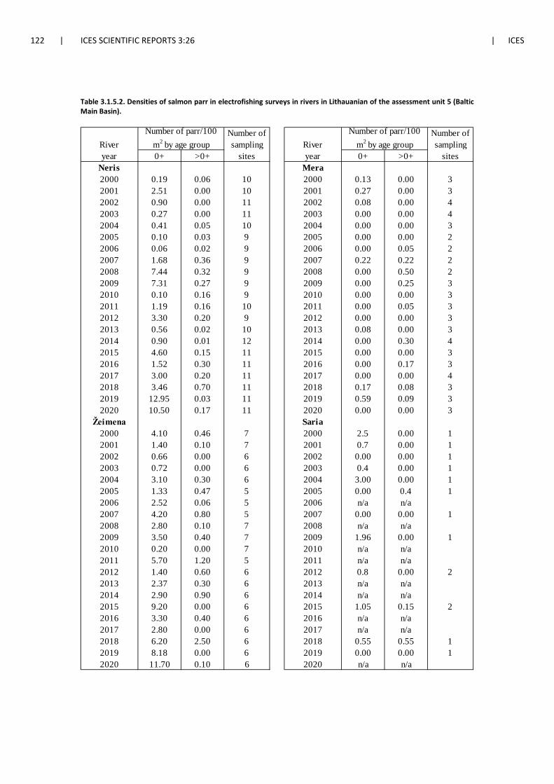
122 | ICES SCIENTIFIC REPORTS 3:26 | ICES
Table 3.1.5.2. Densities of salmon parr in electrofishing surveys in rivers in Lithauanian of the assessment unit 5 (Baltic Main Basin).
Number of Number ofsampling sampling
0+ >0+ sites 0+ >0+ sitesNeris Mera2000 0.19 0.06 10 2000 0.13 0.00 32001 2.51 0.00 10 2001 0.27 0.00 32002 0.90 0.00 11 2002 0.08 0.00 42003 0.27 0.00 11 2003 0.00 0.00 42004 0.41 0.05 10 2004 0.00 0.00 32005 0.10 0.03 9 2005 0.00 0.00 22006 0.06 0.02 9 2006 0.00 0.05 22007 1.68 0.36 9 2007 0.22 0.22 22008 7.44 0.32 9 2008 0.00 0.50 22009 7.31 0.27 9 2009 0.00 0.25 32010 0.10 0.16 9 2010 0.00 0.00 32011 1.19 0.16 10 2011 0.00 0.05 32012 3.30 0.20 9 2012 0.00 0.00 32013 0.56 0.02 10 2013 0.08 0.00 32014 0.90 0.01 12 2014 0.00 0.30 42015 4.60 0.15 11 2015 0.00 0.00 32016 1.52 0.30 11 2016 0.00 0.17 32017 3.00 0.20 11 2017 0.00 0.00 42018 3.46 0.70 11 2018 0.17 0.08 32019 12.95 0.03 11 2019 0.59 0.09 32020 10.50 0.17 11 2020 0.00 0.00 3
Žeimena Saria2000 4.10 0.46 7 2000 2.5 0.00 12001 1.40 0.10 7 2001 0.7 0.00 12002 0.66 0.00 6 2002 0.00 0.00 12003 0.72 0.00 6 2003 0.4 0.00 12004 3.10 0.30 6 2004 3.00 0.00 12005 1.33 0.47 5 2005 0.00 0.4 12006 2.52 0.06 5 2006 n/a n/a2007 4.20 0.80 5 2007 0.00 0.00 12008 2.80 0.10 7 2008 n/a n/a2009 3.50 0.40 7 2009 1.96 0.00 12010 0.20 0.00 7 2010 n/a n/a2011 5.70 1.20 5 2011 n/a n/a2012 1.40 0.60 6 2012 0.8 0.00 22013 2.37 0.30 6 2013 n/a n/a2014 2.90 0.90 6 2014 n/a n/a2015 9.20 0.00 6 2015 1.05 0.15 22016 3.30 0.40 6 2016 n/a n/a2017 2.80 0.00 6 2017 n/a n/a2018 6.20 2.50 6 2018 0.55 0.55 12019 8.18 0.00 6 2019 0.00 0.00 12020 11.70 0.10 6 2020 n/a n/a
River year
Number of parr/100 m2 by age group River
year
Number of parr/100 m2 by age group
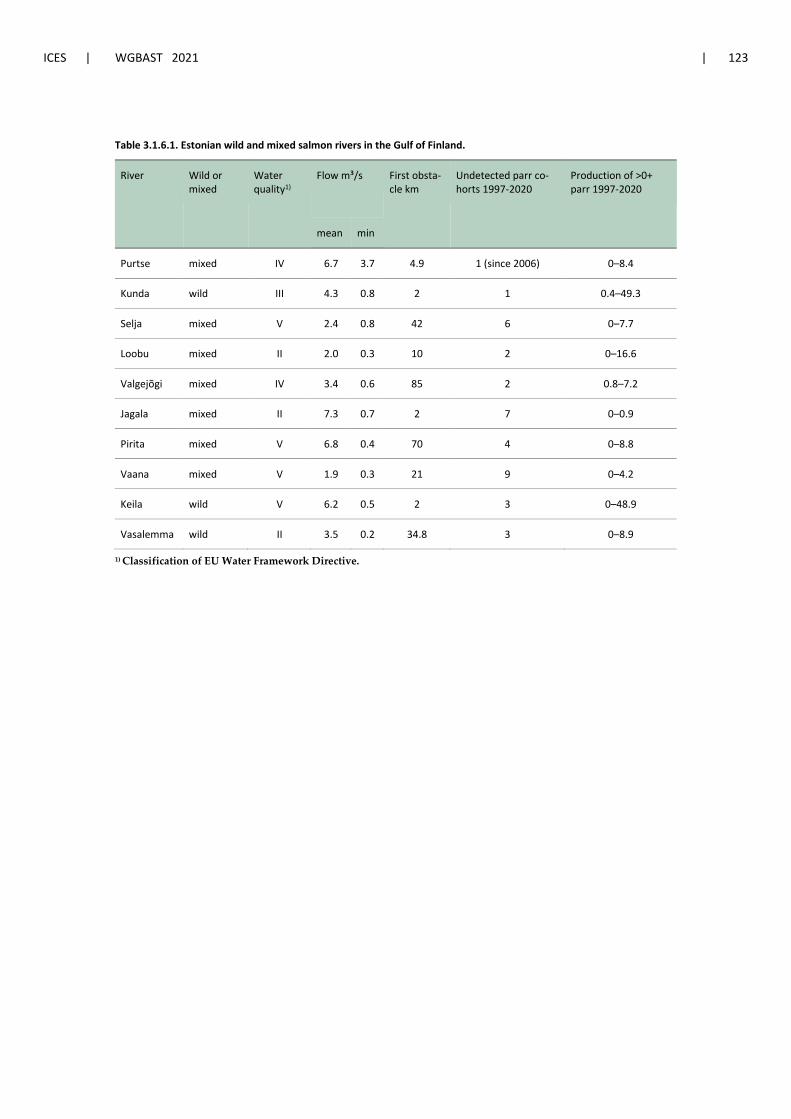
ICES | WGBAST 2021 | 123
Table 3.1.6.1. Estonian wild and mixed salmon rivers in the Gulf of Finland.
River Wild or mixed
Water quality1)
Flow m³/s First obsta-cle km
Undetected parr co-horts 1997-2020
Production of >0+ parr 1997-2020
mean min
Purtse mixed IV 6.7 3.7 4.9 1 (since 2006) 0–8.4
Kunda wild III 4.3 0.8 2 1 0.4–49.3
Selja mixed V 2.4 0.8 42 6 0–7.7
Loobu mixed II 2.0 0.3 10 2 0–16.6
Valgejõgi mixed IV 3.4 0.6 85 2 0.8–7.2
Jagala mixed II 7.3 0.7 2 7 0–0.9
Pirita mixed V 6.8 0.4 70 4 0–8.8
Vaana mixed V 1.9 0.3 21 9 0–4.2
Keila wild V 6.2 0.5 2 3 0–48.9
Vasalemma wild II 3.5 0.2 34.8 3 0–8.9
1) Classification of EU Water Framework Directive.
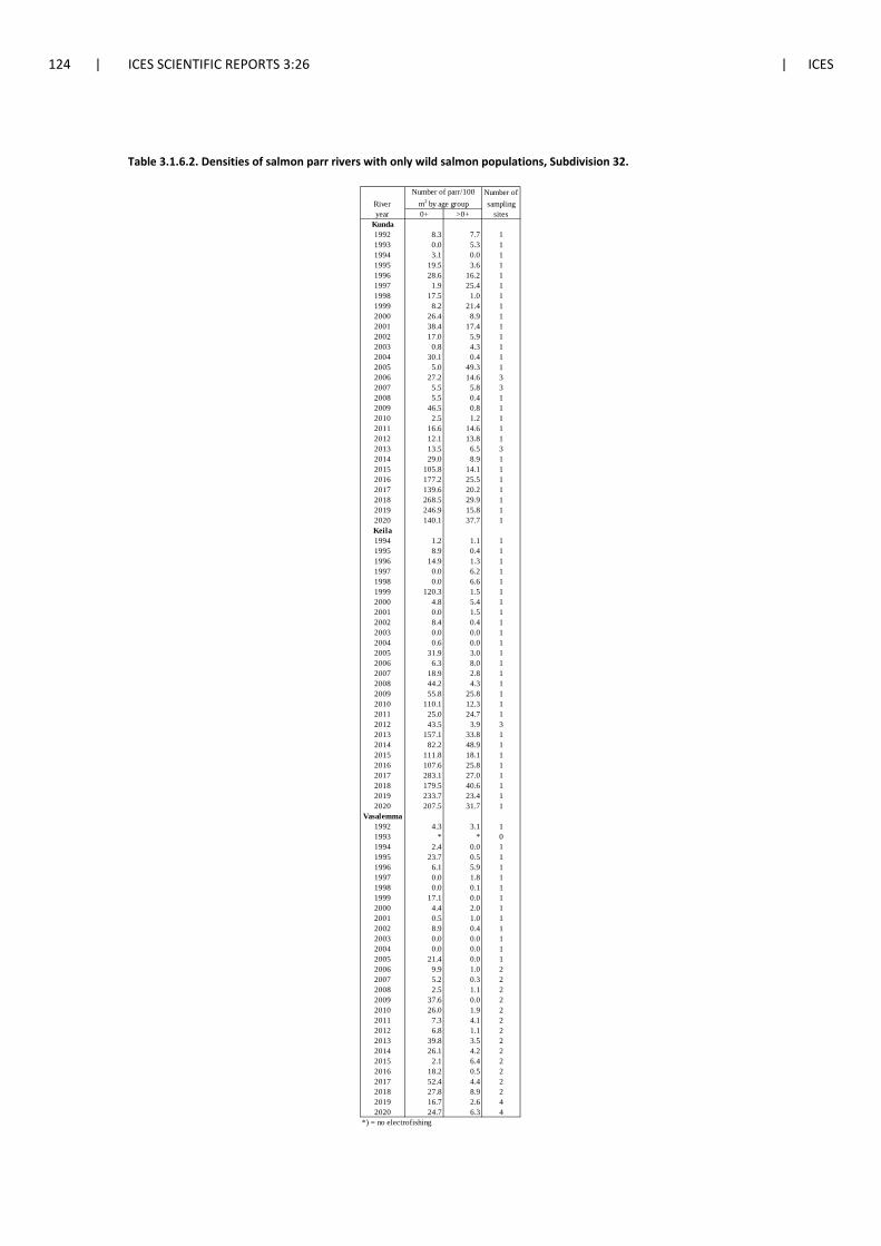
124 | ICES SCIENTIFIC REPORTS 3:26 | ICES
Table 3.1.6.2. Densities of salmon parr rivers with only wild salmon populations, Subdivision 32.
Number ofsampling
0+ >0+ sitesKunda1992 8.3 7.7 11993 0.0 5.3 11994 3.1 0.0 11995 19.5 3.6 11996 28.6 16.2 11997 1.9 25.4 11998 17.5 1.0 11999 8.2 21.4 12000 26.4 8.9 12001 38.4 17.4 12002 17.0 5.9 12003 0.8 4.3 12004 30.1 0.4 12005 5.0 49.3 12006 27.2 14.6 32007 5.5 5.8 32008 5.5 0.4 12009 46.5 0.8 12010 2.5 1.2 12011 16.6 14.6 12012 12.1 13.8 12013 13.5 6.5 32014 29.0 8.9 12015 105.8 14.1 12016 177.2 25.5 12017 139.6 20.2 12018 268.5 29.9 12019 246.9 15.8 12020 140.1 37.7 1Keila1994 1.2 1.1 11995 8.9 0.4 11996 14.9 1.3 11997 0.0 6.2 11998 0.0 6.6 11999 120.3 1.5 12000 4.8 5.4 12001 0.0 1.5 12002 8.4 0.4 12003 0.0 0.0 12004 0.6 0.0 12005 31.9 3.0 12006 6.3 8.0 12007 18.9 2.8 12008 44.2 4.3 12009 55.8 25.8 12010 110.1 12.3 12011 25.0 24.7 12012 43.5 3.9 32013 157.1 33.8 12014 82.2 48.9 12015 111.8 18.1 12016 107.6 25.8 12017 283.1 27.0 12018 179.5 40.6 12019 233.7 23.4 12020 207.5 31.7 1
Vasalemma1992 4.3 3.1 11993 * * 01994 2.4 0.0 11995 23.7 0.5 11996 6.1 5.9 11997 0.0 1.8 11998 0.0 0.1 11999 17.1 0.0 12000 4.4 2.0 12001 0.5 1.0 12002 8.9 0.4 12003 0.0 0.0 12004 0.0 0.0 12005 21.4 0.0 12006 9.9 1.0 22007 5.2 0.3 22008 2.5 1.1 22009 37.6 0.0 22010 26.0 1.9 22011 7.3 4.1 22012 6.8 1.1 22013 39.8 3.5 22014 26.1 4.2 22015 2.1 6.4 22016 18.2 0.5 22017 52.4 4.4 22018 27.8 8.9 22019 16.7 2.6 42020 24.7 6.3 4
*) = no electrofishing
River year
Number of parr/100 m2 by age group
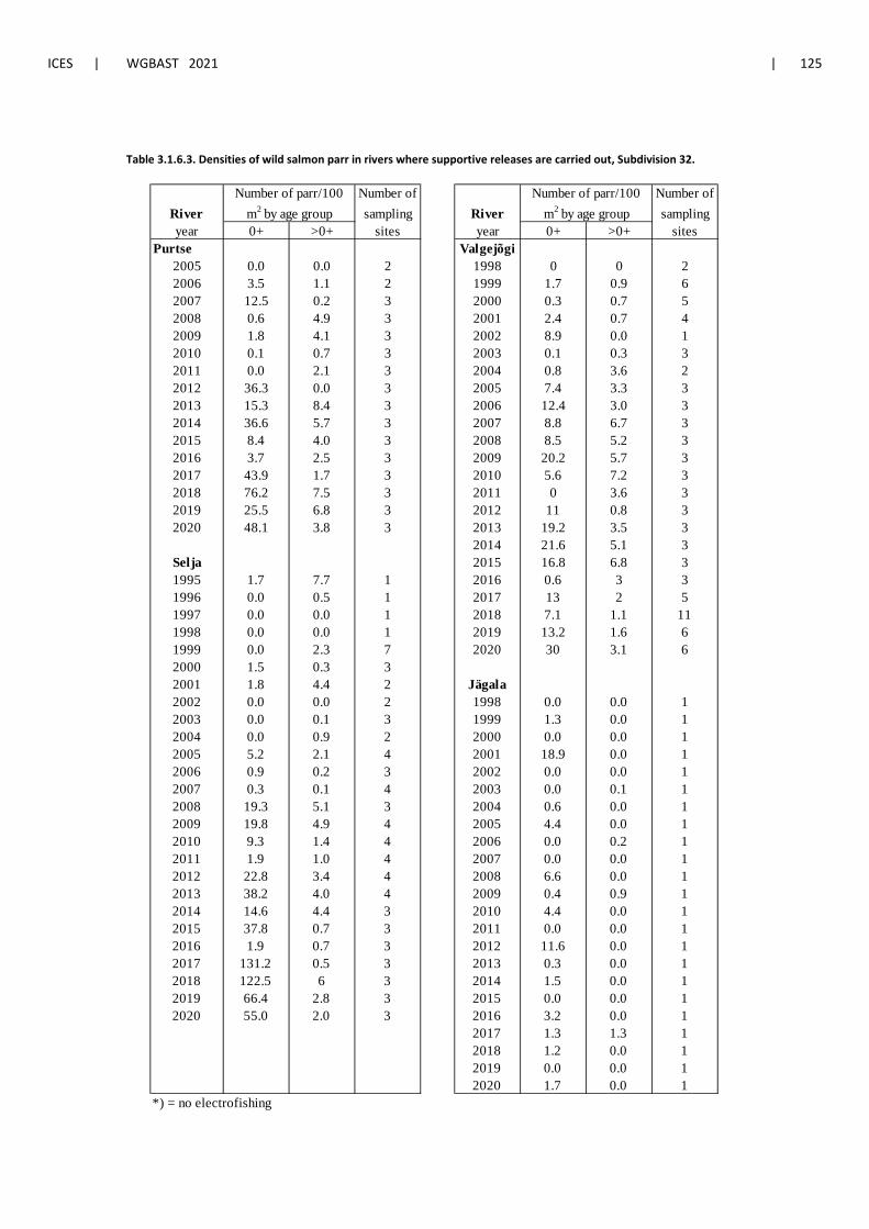
ICES | WGBAST 2021 | 125
Table 3.1.6.3. Densities of wild salmon parr in rivers where supportive releases are carried out, Subdivision 32.
Number of Number ofsampling sampling
0+ >0+ sites 0+ >0+ sitesPurtse Valgejõgi
2005 0.0 0.0 2 1998 0 0 22006 3.5 1.1 2 1999 1.7 0.9 62007 12.5 0.2 3 2000 0.3 0.7 52008 0.6 4.9 3 2001 2.4 0.7 42009 1.8 4.1 3 2002 8.9 0.0 12010 0.1 0.7 3 2003 0.1 0.3 32011 0.0 2.1 3 2004 0.8 3.6 22012 36.3 0.0 3 2005 7.4 3.3 32013 15.3 8.4 3 2006 12.4 3.0 32014 36.6 5.7 3 2007 8.8 6.7 32015 8.4 4.0 3 2008 8.5 5.2 32016 3.7 2.5 3 2009 20.2 5.7 32017 43.9 1.7 3 2010 5.6 7.2 32018 76.2 7.5 3 2011 0 3.6 32019 25.5 6.8 3 2012 11 0.8 32020 48.1 3.8 3 2013 19.2 3.5 3
2014 21.6 5.1 3Selja 2015 16.8 6.8 31995 1.7 7.7 1 2016 0.6 3 31996 0.0 0.5 1 2017 13 2 51997 0.0 0.0 1 2018 7.1 1.1 111998 0.0 0.0 1 2019 13.2 1.6 61999 0.0 2.3 7 2020 30 3.1 62000 1.5 0.3 32001 1.8 4.4 2 Jägala2002 0.0 0.0 2 1998 0.0 0.0 12003 0.0 0.1 3 1999 1.3 0.0 12004 0.0 0.9 2 2000 0.0 0.0 12005 5.2 2.1 4 2001 18.9 0.0 12006 0.9 0.2 3 2002 0.0 0.0 12007 0.3 0.1 4 2003 0.0 0.1 12008 19.3 5.1 3 2004 0.6 0.0 12009 19.8 4.9 4 2005 4.4 0.0 12010 9.3 1.4 4 2006 0.0 0.2 12011 1.9 1.0 4 2007 0.0 0.0 12012 22.8 3.4 4 2008 6.6 0.0 12013 38.2 4.0 4 2009 0.4 0.9 12014 14.6 4.4 3 2010 4.4 0.0 12015 37.8 0.7 3 2011 0.0 0.0 12016 1.9 0.7 3 2012 11.6 0.0 12017 131.2 0.5 3 2013 0.3 0.0 12018 122.5 6 3 2014 1.5 0.0 12019 66.4 2.8 3 2015 0.0 0.0 12020 55.0 2.0 3 2016 3.2 0.0 1
2017 1.3 1.3 12018 1.2 0.0 12019 0.0 0.0 12020 1.7 0.0 1
*) = no electrofishing
River year
Number of parr/100 m2 by age group River
year
Number of parr/100 m2 by age group
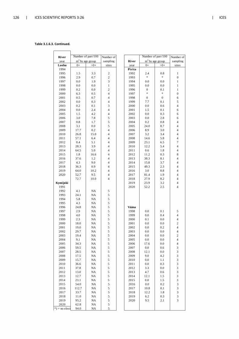
126 | ICES SCIENTIFIC REPORTS 3:26 | ICES
Table 3.1.6.3. Continued.
Number of Number ofsampling sampling
Loobu 0+ >0+ sites 0+ >0+ sites1994 Pirita1995 1.5 3.3 2 1992 2.4 0.8 11996 2.9 0.7 2 1993 * * 01997 0.0 1.9 3 1994 0.0 0.0 11998 0.0 0.0 1 1995 0.0 0.0 11999 0.2 0.0 2 1996 0 0.1 12000 6.3 0.5 4 1997 * * 02001 0.5 0.7 4 1998 0 0 62002 0.0 0.3 4 1999 7.7 0.1 52003 0.2 0.1 3 2000 0.0 0.6 42004 0.0 2.4 4 2001 1.5 0.1 62005 1.5 4.2 4 2002 0.0 0.3 62006 3.0 7.8 5 2003 0.0 2.8 62007 0.8 1.7 5 2004 0.2 0.8 42008 3.1 0.0 5 2005 24.0 8.7 42009 17.7 0.2 4 2006 8.9 3.0 42010 26.8 15.0 4 2007 3.2 3.4 42011 57.1 6.4 4 2008 14.6 5.8 42012 0.4 5.1 4 2009 23.1 6.5 72013 28.3 3.9 4 2010 12.2 5.4 42014 64.5 5.0 4 2011 0.6 1.8 42015 1.8 16.6 4 2012 11.2 0.3 82016 37.6 1.2 4 2013 38.3 8.1 42017 4.3 9.0 4 2014 15.8 3.7 42018 36.3 0.9 4 2015 49.3 2.3 42019 64.0 10.2 4 2016 3.0 8.8 42020 52.7 9.5 4 2017 81.4 1.9 4
72.7 10.0 4 2018 27.9 8.2 4Kymijoki 2019 23.9 3.2 4
1991 2020 52.2 2.5 41992 4.1 NA 51993 24.1 NA 51994 5.8 NA 51995 4.3 NA 51996 24.8 NA 5 Vääna1997 2.9 NA 5 1998 0.0 0.1 51998 4.0 NA 5 1999 0.0 0.4 41999 2.3 NA 5 2000 0.1 0.0 42000 18.0 NA 5 2001 0.0 0.0 22001 19.0 NA 5 2002 0.0 0.2 42002 29.7 NA 5 2003 0.0 0.0 42003 19.4 NA 5 2004 0.0 0.0 22004 9.1 NA 5 2005 0.0 0.0 42005 34.3 NA 5 2006 17.6 0.0 42006 59.5 NA 5 2007 0.0 0.6 32007 28.5 NA 5 2008 12.1 0.0 32008 17.5 NA 5 2009 9.0 4.2 32009 15.7 NA 5 2010 0.0 1.1 32010 36.6 NA 5 2011 0.0 0.3 32011 37.8 NA 5 2012 3.3 0.0 32012 13.0 NA 5 2013 4.7 0.6 32013 12.7 NA 5 2014 12.1 1.5 32014 23.1 NA 5 2015 0.0 1.5 32015 54.0 NA 5 2016 0.0 0.2 32016 112.7 NA 5 2017 10.8 0.1 32017 33.7 NA 5 2018 12.2 1.8 32018 11.0 NA 5 2019 6.2 0.3 32019 95.2 NA 5 2020 9.5 2.1 32020 62.8 NA 5
*) = no electr 94.0 NA 5
River year
Number of parr/100 m2 by age group River
year
Number of parr/100 m2 by age group
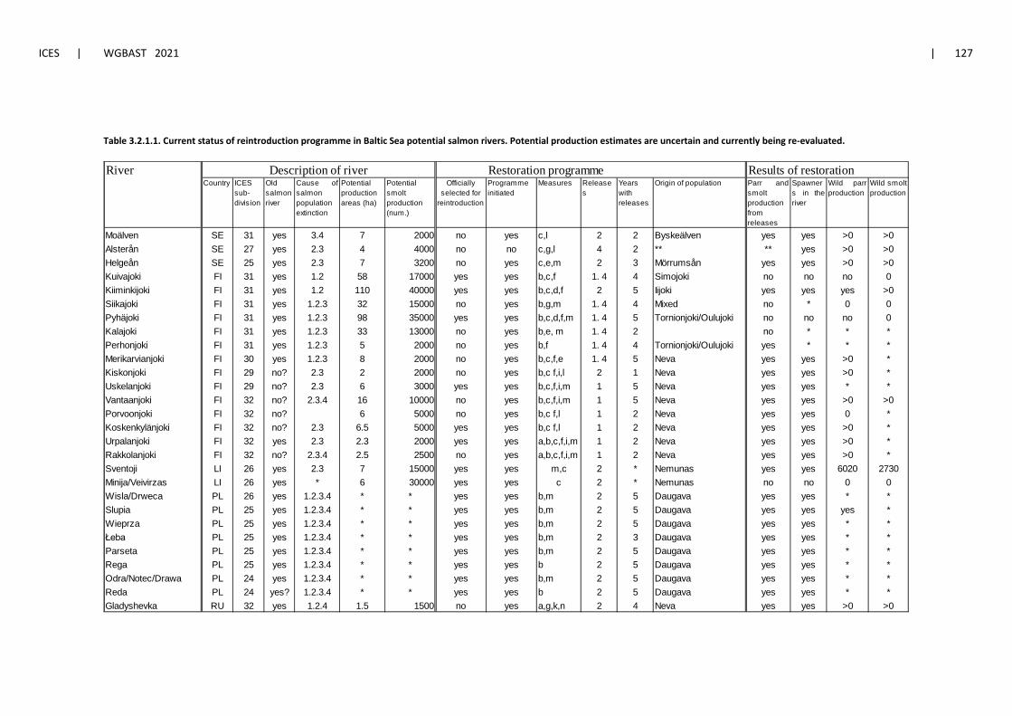
ICES | WGBAST 2021 | 127
Table 3.2.1.1. Current status of reintroduction programme in Baltic Sea potential salmon rivers. Potential production estimates are uncertain and currently being re-evaluated.
River Restoration programme Results of restorationCountry ICES
sub- division
Old salmon river
Cause ofsalmon population extinction
Potential production areas (ha)
Potential smolt production (num.)
Officially selected for
reintroduction
Programme initiated
Measures Releases
Years with releases
Origin of population Parr andsmolt production from releases
Spawners in theriver
Wild parrproduction
Wild smoltproduction
Moälven SE 31 yes 3.4 7 2000 no yes c,l 2 2 Byskeälven yes yes >0 >0Alsterån SE 27 yes 2.3 4 4000 no no c,g,l 4 2 ** ** yes >0 >0Helgeån SE 25 yes 2.3 7 3200 no yes c,e,m 2 3 Mörrumsån yes yes >0 >0Kuivajoki FI 31 yes 1.2 58 17000 yes yes b,c,f 1. 4 4 Simojoki no no no 0Kiiminkijoki FI 31 yes 1.2 110 40000 yes yes b,c,d,f 2 5 Iijoki yes yes yes >0Siikajoki FI 31 yes 1.2.3 32 15000 no yes b,g,m 1. 4 4 Mixed no * 0 0Pyhäjoki FI 31 yes 1.2.3 98 35000 yes yes b,c,d,f,m 1. 4 5 Tornionjoki/Oulujoki no no no 0Kalajoki FI 31 yes 1.2.3 33 13000 no yes b,e, m 1. 4 2 no * * *Perhonjoki FI 31 yes 1.2.3 5 2000 no yes b,f 1. 4 4 Tornionjoki/Oulujoki yes * * *Merikarvianjoki FI 30 yes 1.2.3 8 2000 no yes b,c,f,e 1. 4 5 Neva yes yes >0 *Kiskonjoki FI 29 no? 2.3 2 2000 no yes b,c f,i,l 2 1 Neva yes yes >0 *Uskelanjoki FI 29 no? 2.3 6 3000 yes yes b,c,f,i,m 1 5 Neva yes yes * *Vantaanjoki FI 32 no? 2.3.4 16 10000 no yes b,c,f,i,m 1 5 Neva yes yes >0 >0Porvoonjoki FI 32 no? 6 5000 no yes b,c f,l 1 2 Neva yes yes 0 *Koskenkylänjoki FI 32 no? 2.3 6.5 5000 yes yes b,c f,l 1 2 Neva yes yes >0 *Urpalanjoki FI 32 yes 2.3 2.3 2000 yes yes a,b,c,f,i,m 1 2 Neva yes yes >0 *Rakkolanjoki FI 32 no? 2.3.4 2.5 2500 no yes a,b,c,f,i,m 1 2 Neva yes yes >0 *Sventoji LI 26 yes 2.3 7 15000 yes yes m,c 2 * Nemunas yes yes 6020 2730Minija/Veivirzas LI 26 yes * 6 30000 yes yes c 2 * Nemunas no no 0 0Wisla/Drweca PL 26 yes 1.2.3.4 * * yes yes b,m 2 5 Daugava yes yes * *Slupia PL 25 yes 1.2.3.4 * * yes yes b,m 2 5 Daugava yes yes yes *Wieprza PL 25 yes 1.2.3.4 * * yes yes b,m 2 5 Daugava yes yes * *Łeba PL 25 yes 1.2.3.4 * * yes yes b,m 2 3 Daugava yes yes * *Parseta PL 25 yes 1.2.3.4 * * yes yes b,m 2 5 Daugava yes yes * *Rega PL 25 yes 1.2.3.4 * * yes yes b 2 5 Daugava yes yes * *Odra/Notec/Drawa PL 24 yes 1.2.3.4 * * yes yes b,m 2 5 Daugava yes yes * *Reda PL 24 yes? 1.2.3.4 * * yes yes b 2 5 Daugava yes yes * *Gladyshevka RU 32 yes 1.2.4 1.5 1500 no yes a,g,k,n 2 4 Neva yes yes >0 >0
Description of river
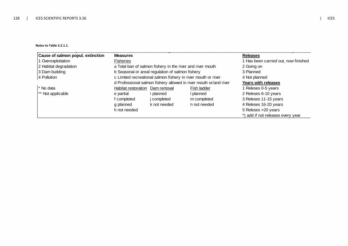
128 | ICES SCIENTIFIC REPORTS 3:26 | ICES
Notes to Table 3.2.1.1.
Cause of salmon popul. extinction Measures Releases1 Overexploitation Fisheries 1 Has been carried out, now finished2 Habitat degradation a Total ban of salmon fishery in the river and river mouth 2 Going on3 Dam building b Seasonal or areal regulation of salmon fishery 3 Planned4 Pollution c Limited recreational salmon fishery in river mouth or river 4 Not planned
d Professional salmon fishery allowed in river mouth or/and river Years with releases* No data Habitat restoration Dam removal Fish ladder 1 Releses 0-5 years** Not applicable e partial i planned l planned 2 Releses 6-10 years
f completed j completed m completed 3 Releses 11-15 yearsg planned k not needed n not needed 4 Releses 16-20 yearsh not needed 5 Releses >20 years
*) add if not releases every year
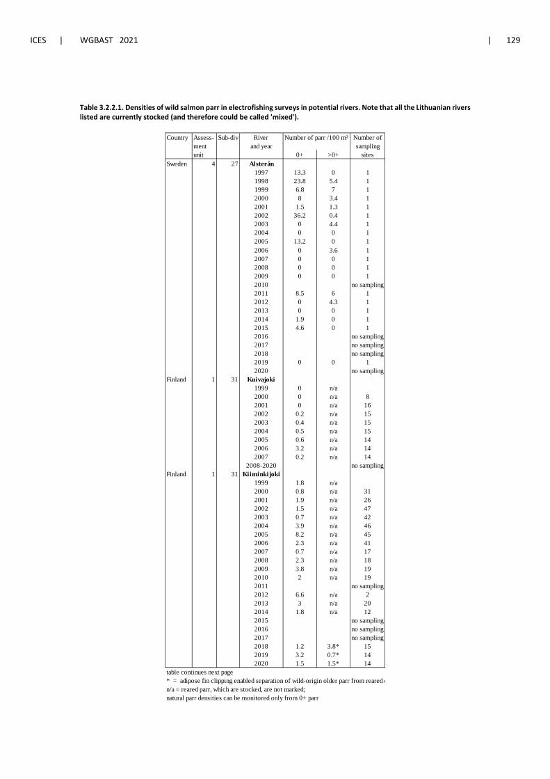
ICES | WGBAST 2021 | 129
Table 3.2.2.1. Densities of wild salmon parr in electrofishing surveys in potential rivers. Note that all the Lithuanian rivers listed are currently stocked (and therefore could be called 'mixed').
Country Assess- Sub-div River Number ofment and year samplingunit 0+ >0+ sites
Sweden 4 27 Alsterån1997 13.3 0 11998 23.8 5.4 11999 6.8 7 12000 8 3.4 12001 1.5 1.3 12002 36.2 0.4 12003 0 4.4 12004 0 0 12005 13.2 0 12006 0 3.6 12007 0 0 12008 0 0 12009 0 0 12010 no sampling2011 8.5 6 12012 0 4.3 12013 0 0 12014 1.9 0 12015 4.6 0 12016 no sampling2017 no sampling2018 no sampling2019 0 0 12020 no sampling
Finland 1 31 Kuivajoki1999 0 n/a2000 0 n/a 82001 0 n/a 162002 0.2 n/a 152003 0.4 n/a 152004 0.5 n/a 152005 0.6 n/a 142006 3.2 n/a 142007 0.2 n/a 14
2008-2020 no samplingFinland 1 31 Kiiminkijoki
1999 1.8 n/a2000 0.8 n/a 312001 1.9 n/a 262002 1.5 n/a 472003 0.7 n/a 422004 3.9 n/a 462005 8.2 n/a 452006 2.3 n/a 412007 0.7 n/a 172008 2.3 n/a 182009 3.8 n/a 192010 2 n/a 192011 no sampling2012 6.6 n/a 22013 3 n/a 202014 1.8 n/a 122015 no sampling2016 no sampling2017 no sampling2018 1.2 3.8* 152019 3.2 0.7* 142020 1.5 1.5* 14
table continues next page* = adipose fin clipping enabled separation of wild-origin older parr from reared o n/a = reared parr, which are stocked, are not marked; natural parr densities can be monitored only from 0+ parr
Number of parr /100 m²
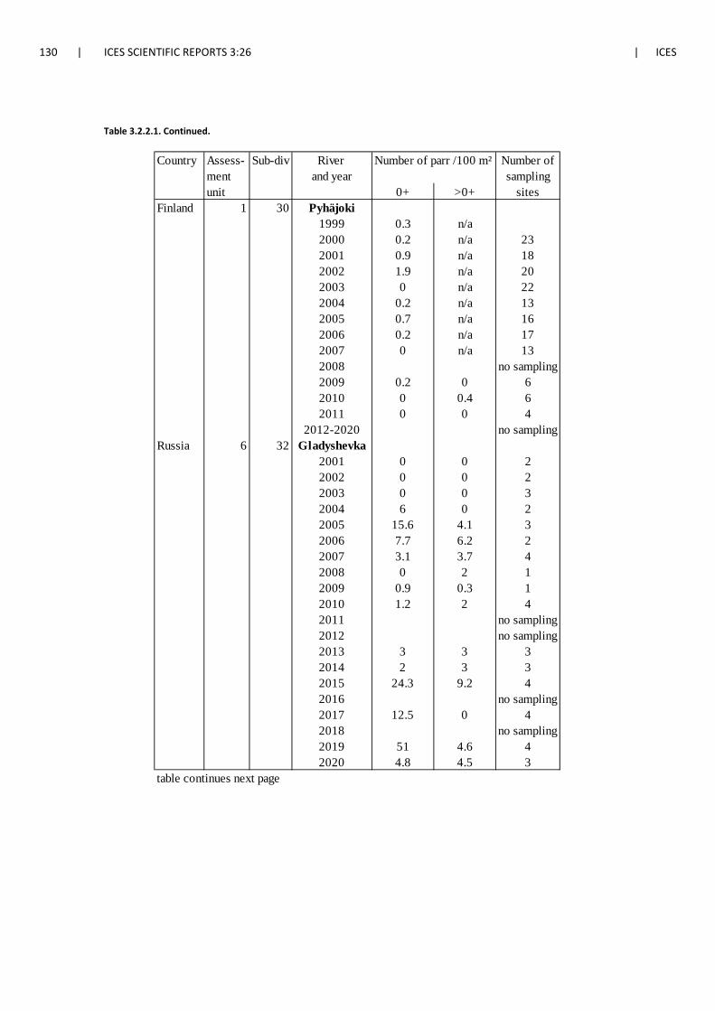
130 | ICES SCIENTIFIC REPORTS 3:26 | ICES
Table 3.2.2.1. Continued.
Country Assess- Sub-div River Number ofment and year samplingunit 0+ >0+ sites
Finland 1 30 Pyhäjoki1999 0.3 n/a2000 0.2 n/a 232001 0.9 n/a 182002 1.9 n/a 202003 0 n/a 222004 0.2 n/a 132005 0.7 n/a 162006 0.2 n/a 172007 0 n/a 132008 no sampling2009 0.2 0 62010 0 0.4 62011 0 0 4
2012-2020 no samplingRussia 6 32 Gladyshevka
2001 0 0 22002 0 0 22003 0 0 32004 6 0 22005 15.6 4.1 32006 7.7 6.2 22007 3.1 3.7 42008 0 2 12009 0.9 0.3 12010 1.2 2 42011 no sampling2012 no sampling2013 3 3 32014 2 3 32015 24.3 9.2 42016 no sampling2017 12.5 0 42018 no sampling2019 51 4.6 42020 4.8 4.5 3
table continues next page
Number of parr /100 m²
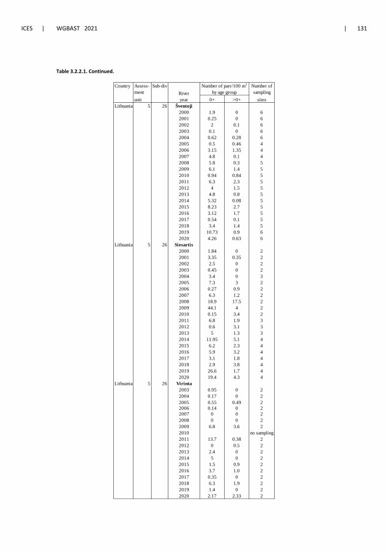
ICES | WGBAST 2021 | 131
Table 3.2.2.1. Continued.
Country Assess- Sub-div Number ofment samplingunit 0+ >0+ sites
Lithuania 5 26 Šventoji2000 1.9 0 62001 0.25 0 62002 2 0.1 62003 0.1 0 62004 0.62 0.28 62005 0.5 0.46 42006 3.15 1.35 42007 4.8 0.1 42008 5.8 0.3 52009 6.1 1.4 52010 0.94 0.84 52011 6.3 2.3 52012 4 1.5 52013 4.8 0.8 52014 5.32 0.08 52015 8.23 2.7 52016 3.12 1.7 52017 0.54 0.1 52018 3.4 1.4 52019 10.73 0.9 62020 4.26 0.63 6
Lithuania 5 26 Siesartis2000 1.84 0 22001 3.35 0.35 22002 2.5 0 22003 0.45 0 22004 3.4 0 32005 7.3 3 22006 0.27 0.9 22007 6.3 1.2 22008 18.9 17.5 22009 44.1 4 22010 0.15 3.4 22011 6.8 1.9 32012 0.6 3.1 32013 5 1.3 32014 11.95 5.1 42015 6.2 2.3 42016 5.9 3.2 42017 3.1 1.8 42018 2.9 3.8 42019 26.6 1.7 42020 19.4 4.3 4
Lithuania 5 26 Virinta2003 0.95 0 22004 0.17 0 22005 0.55 0.49 22006 0.14 0 22007 0 0 22008 0 0 22009 6.8 3.6 22010 no sampling2011 13.7 0.38 22012 0 0.5 22013 2.4 0 22014 5 0 22015 1.5 0.9 22016 3.7 1.0 22017 0.35 0 22018 6.3 1.9 22019 1.4 0 22020 2.17 2.33 2
River year
Number of parr/100 m2
by age group
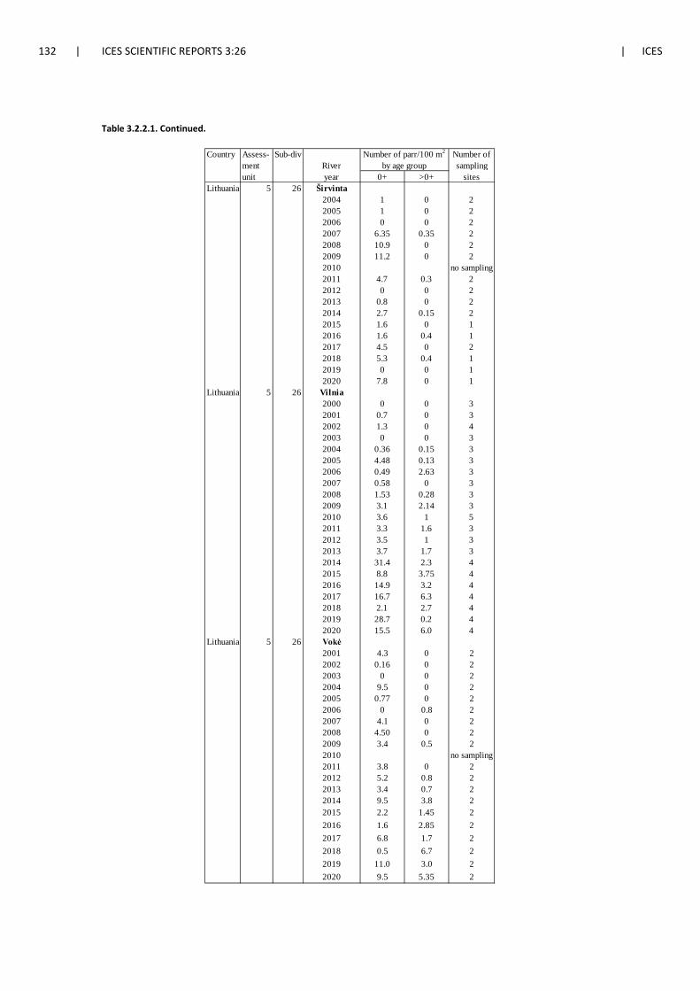
132 | ICES SCIENTIFIC REPORTS 3:26 | ICES
Table 3.2.2.1. Continued.
Country Assess- Sub-div Number ofment samplingunit 0+ >0+ sites
Lithuania 5 26 Širvinta2004 1 0 22005 1 0 22006 0 0 22007 6.35 0.35 22008 10.9 0 22009 11.2 0 22010 no sampling2011 4.7 0.3 22012 0 0 22013 0.8 0 22014 2.7 0.15 22015 1.6 0 12016 1.6 0.4 12017 4.5 0 22018 5.3 0.4 12019 0 0 12020 7.8 0 1
Lithuania 5 26 Vilnia2000 0 0 32001 0.7 0 32002 1.3 0 42003 0 0 32004 0.36 0.15 32005 4.48 0.13 32006 0.49 2.63 32007 0.58 0 32008 1.53 0.28 32009 3.1 2.14 32010 3.6 1 52011 3.3 1.6 32012 3.5 1 32013 3.7 1.7 32014 31.4 2.3 42015 8.8 3.75 42016 14.9 3.2 42017 16.7 6.3 42018 2.1 2.7 42019 28.7 0.2 42020 15.5 6.0 4
Lithuania 5 26 Vokė2001 4.3 0 22002 0.16 0 22003 0 0 22004 9.5 0 22005 0.77 0 22006 0 0.8 22007 4.1 0 22008 4.50 0 22009 3.4 0.5 22010 no sampling2011 3.8 0 22012 5.2 0.8 22013 3.4 0.7 22014 9.5 3.8 22015 2.2 1.45 22016 1.6 2.85 22017 6.8 1.7 22018 0.5 6.7 22019 11.0 3.0 22020 9.5 5.35 2
River year
Number of parr/100 m2
by age group
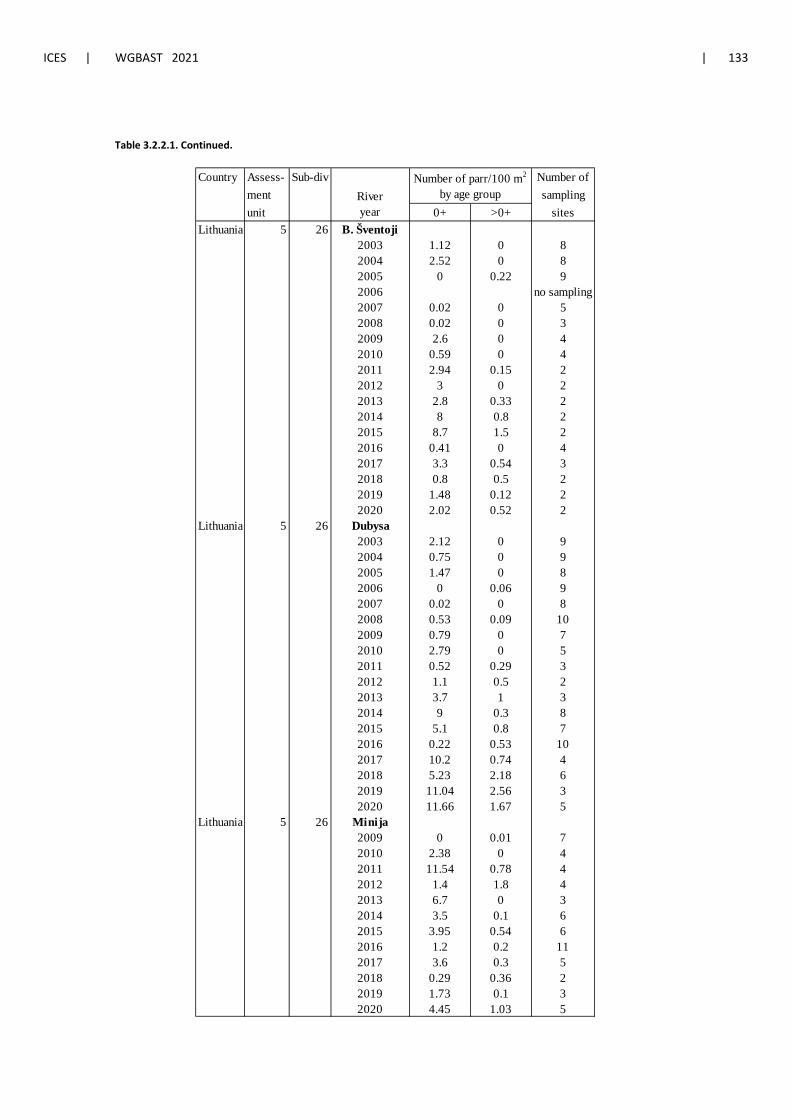
ICES | WGBAST 2021 | 133
Table 3.2.2.1. Continued.
Country Assess- Sub-div Number ofment samplingunit 0+ >0+ sites
Lithuania 5 26 B. Šventoji2003 1.12 0 82004 2.52 0 82005 0 0.22 92006 no sampling2007 0.02 0 52008 0.02 0 32009 2.6 0 42010 0.59 0 42011 2.94 0.15 22012 3 0 22013 2.8 0.33 22014 8 0.8 22015 8.7 1.5 22016 0.41 0 42017 3.3 0.54 32018 0.8 0.5 22019 1.48 0.12 22020 2.02 0.52 2
Lithuania 5 26 Dubysa2003 2.12 0 92004 0.75 0 92005 1.47 0 82006 0 0.06 92007 0.02 0 82008 0.53 0.09 102009 0.79 0 72010 2.79 0 52011 0.52 0.29 32012 1.1 0.5 22013 3.7 1 32014 9 0.3 82015 5.1 0.8 72016 0.22 0.53 102017 10.2 0.74 42018 5.23 2.18 62019 11.04 2.56 32020 11.66 1.67 5
Lithuania 5 26 Minija2009 0 0.01 72010 2.38 0 42011 11.54 0.78 42012 1.4 1.8 42013 6.7 0 32014 3.5 0.1 62015 3.95 0.54 62016 1.2 0.2 112017 3.6 0.3 52018 0.29 0.36 22019 1.73 0.1 32020 4.45 1.03 5
River year
Number of parr/100 m2
by age group
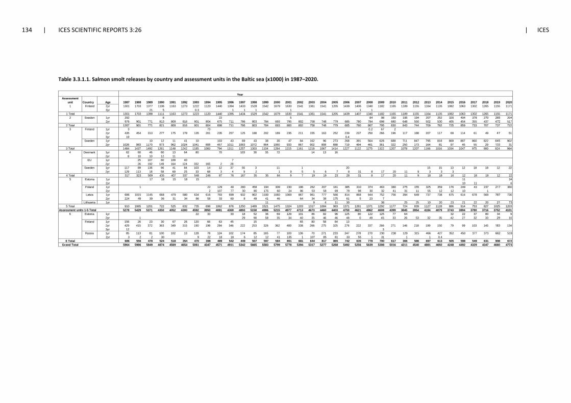
134 | ICES SCIENTIFIC REPORTS 3:26 | ICES
Table 3.3.1.1. Salmon smolt releases by country and assessment units in the Baltic sea (x1000) in 1987–2020.
Assessment unit Country Age 1987 1988 1989 1990 1991 1992 1993 1994 1995 1996 1997 1998 1999 2000 2001 2002 2003 2004 2005 2006 2007 2008 2009 2010 2011 2012 2013 2014 2015 2016 2017 2018 2019 2020
1 Finland 2yr 1301 1703 1377 1106 1163 1273 1222 1120 1440 1394 1433 1528 1542 1679 1630 1541 1361 1541 1205 1439 1406 1340 1182 1165 1189 1155 1164 1135 1082 1063 1302 1265 1155 11713yr 21 5 0.3 1 1 1 1 1 1
1 Total 1301 1703 1398 1111 1163 1273 1223 1120 1440 1395 1434 1529 1542 1679 1630 1541 1361 1541 1205 1439 1407 1340 1182 1165 1189 1155 1164 1135 1082 1063 1302 1265 1155 11712 Sweden 1yr 292 8 22 5 84 98 150 195 194 207 252 320 404 378 270 265 204
2yr 976 901 771 813 809 816 901 804 675 711 786 803 784 693 795 802 758 748 779 685 780 784 698 680 648 550 502 530 405 454 355 437 472 5172 Total 1267 901 771 821 809 816 901 804 698 711 786 803 784 693 800 802 758 748 779 685 780 867 795 830 843 744 709 782 725 859 733 707 737 722
3 Finland 1yr 3 73 0.2 67 22yr 435 454 313 277 175 178 135 201 235 257 125 188 202 189 235 211 155 163 252 239 237 250 266 196 117 188 207 117 69 114 61 49 47 513yr 19 0.4
Sweden 1yr 10 12 11 41 10 103 43 69 43 38 35 47 84 162 96 273 268 391 564 628 688 711 847 795 818 869 887 860 822 645 9022yr 1026 983 1170 973 962 1024 1041 808 457 1011 1063 1072 864 1060 933 867 902 808 888 719 494 461 361 322 250 173 164 81 97 45 55 29 133 31
3 Total 1484 1437 1492 1261 1148 1242 1185 1083 794 1311 1257 1303 1104 1284 1215 1161 1218 1067 1414 1227 1122 1275 1322 1207 1078 1207 1166 1016 1034 1047 975 900 824 9844 Denmark 1yr 62 60 46 60 13 64 80 70 103 30 35 72 14 13 16
2yr 8 10 10 12 11EU 1yr 25 107 60 109 40 7
2yr 26 192 149 164 124 332 165 2 28Sweden 1yr 117 89 136 96 41 84 103 14 12 37 55 3 11 1 20 15 15 13 12 18 18 12 22
2yr 129 113 18 58 69 25 33 68 3 4 9 2 1 9 5 5 6 7 8 31 8 17 20 11 9 3 3 34 Total 317 323 509 435 407 337 548 246 87 76 167 35 35 84 9 7 19 19 23 28 31 8 17 20 11 9 18 18 16 12 18 18 12 22
5 1yr 17 18 15 18 15 11 342yr 10 11 6
Poland 1yr 1 22 129 40 280 458 194 309 230 186 262 207 161 385 310 374 463 380 275 155 325 359 176 249 43 237 217 3602yr 2 107 77 30 80 175 60 24 86 53 58 69 79 98 30 32 41 31 11 55 12 12 10 1
Latvia 1yr 686 1015 1145 668 479 580 634 616 793 699 932 902 1100 1060 1069 867 961 777 566 814 868 944 752 756 394 649 737 738 675 614 678 569 787 7302yr 224 49 39 36 31 34 86 58 33 60 8 49 41 46 64 34 38 175 61 5 23 7
Lithuania 1yr 11 9 4 11 30 38 25 25 10 20 23 21 22 20 21 735 Total 910 1065 1201 722 525 632 735 698 1062 876 1250 1489 1521 1475 1324 1203 1317 1084 983 1371 1281 1371 1292 1177 724 839 1127 1128 886 914 753 827 1025 1203
Assessment units 1-5 Total 5278 5429 5371 4350 4052 4300 4592 3950 4081 4369 4893 5158 4986 5215 4977 4713 4673 4460 4403 4750 4621 4862 4608 4399 3845 3954 4184 4079 3743 3894 3780 3716 3752 41016 Estonia 1yr 22 33 30 18 52 36 69 129 101 86 82 96 125 80 122 125 77 64 32 22 37 80 34 9
2yr 1 29 90 58 35 34 40 35 46 46 48 0 49 45 33 26 53 32 35 42 27 32 33 29 10Finland 1yr 156 26 23 30 67 26 120 66 63 45 15 65 80 58 84 13
2yr 429 415 372 363 349 315 190 198 284 346 222 253 326 362 400 338 266 275 325 276 222 337 266 271 146 218 199 150 79 99 103 145 183 1343yr 12 3
Russia 1yr 85 113 81 100 102 13 128 78 124 102 174 85 165 77 103 136 70 271 233 247 278 270 230 238 129 315 466 427 352 450 377 373 662 5192yr 3 2 2 30 9 22 18 18 6 12 12 41 135 1 107 85 81 33 55 1 31 1 1 0.4
6 Total 686 556 478 524 518 354 470 398 489 542 449 507 597 584 801 681 644 817 865 742 635 778 700 617 366 586 697 613 505 598 549 631 908 672Grand Total 5964 5986 5849 4874 4569 4654 5061 4347 4571 4911 5342 5665 5583 5799 5778 5394 5317 5277 5268 5492 5256 5639 5308 5016 4211 4540 4881 4692 4248 4492 4329 4347 4660 4773
Year
Estonia
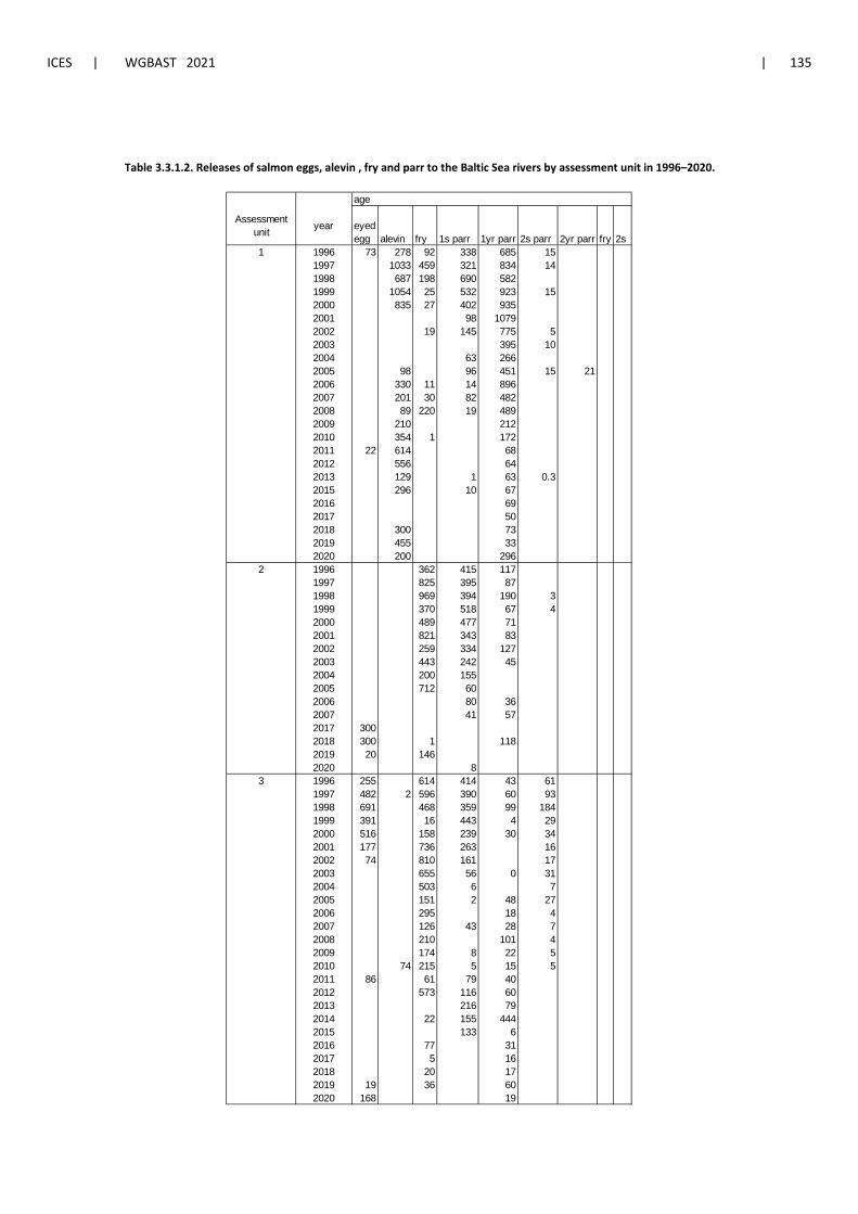
ICES | WGBAST 2021 | 135
Table 3.3.1.2. Releases of salmon eggs, alevin , fry and parr to the Baltic Sea rivers by assessment unit in 1996–2020.
age
Assessment unit year eyed
egg alevin fry 1s parr 1yr parr 2s parr 2yr parr fry 2s1 1996 73 278 92 338 685 15
1997 1033 459 321 834 141998 687 198 690 5821999 1054 25 532 923 152000 835 27 402 9352001 98 10792002 19 145 775 52003 395 102004 63 2662005 98 96 451 15 212006 330 11 14 8962007 201 30 82 4822008 89 220 19 4892009 210 2122010 354 1 1722011 22 614 682012 556 642013 129 1 63 0.32015 296 10 672016 692017 502018 300 732019 455 332020 200 296
2 1996 362 415 1171997 825 395 871998 969 394 190 31999 370 518 67 42000 489 477 712001 821 343 832002 259 334 1272003 443 242 452004 200 1552005 712 602006 80 362007 41 572017 3002018 300 1 1182019 20 1462020 8
3 1996 255 614 414 43 611997 482 2 596 390 60 931998 691 468 359 99 1841999 391 16 443 4 292000 516 158 239 30 342001 177 736 263 162002 74 810 161 172003 655 56 0 312004 503 6 72005 151 2 48 272006 295 18 42007 126 43 28 72008 210 101 42009 174 8 22 52010 74 215 5 15 52011 86 61 79 402012 573 116 602013 216 792014 22 155 4442015 133 62016 77 312017 5 162018 20 172019 19 36 602020 168 19
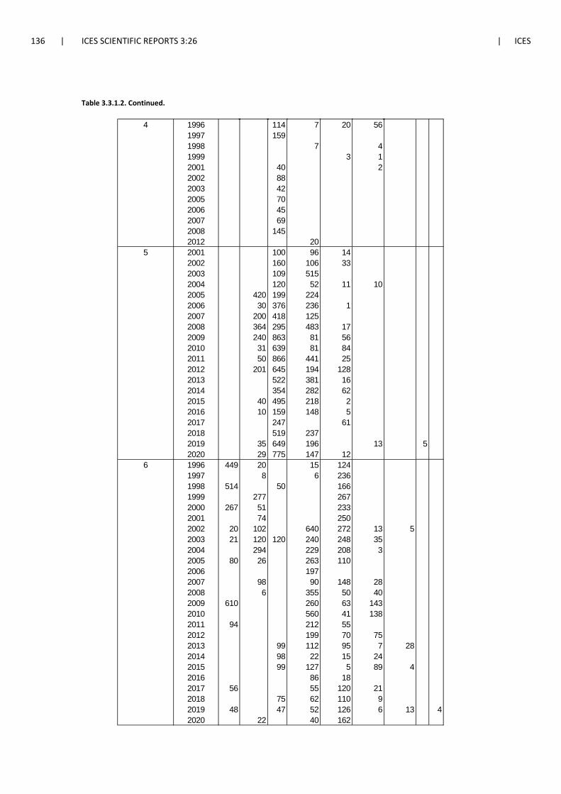
136 | ICES SCIENTIFIC REPORTS 3:26 | ICES
Table 3.3.1.2. Continued.
4 1996 114 7 20 561997 1591998 7 41999 3 12001 40 22002 882003 422005 702006 452007 692008 1452012 20
5 2001 100 96 142002 160 106 332003 109 5152004 120 52 11 102005 420 199 2242006 30 376 236 12007 200 418 1252008 364 295 483 172009 240 863 81 562010 31 639 81 842011 50 866 441 252012 201 645 194 1282013 522 381 162014 354 282 622015 40 495 218 22016 10 159 148 52017 247 612018 519 2372019 35 649 196 13 52020 29 775 147 12
6 1996 449 20 15 1241997 8 6 2361998 514 50 1661999 277 2672000 267 51 2332001 74 2502002 20 102 640 272 13 52003 21 120 120 240 248 352004 294 229 208 32005 80 26 263 1102006 1972007 98 90 148 282008 6 355 50 402009 610 260 63 1432010 560 41 1382011 94 212 552012 199 70 752013 99 112 95 7 282014 98 22 15 242015 99 127 5 89 42016 86 182017 56 55 120 212018 75 62 110 92019 48 47 52 126 6 13 42020 22 40 162
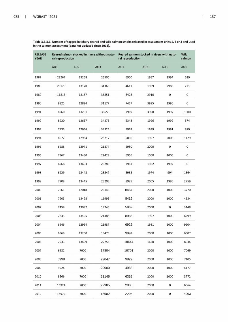
ICES | WGBAST 2021 | 137
Table 3.3.3.1. Number of tagged hatchery-reared and wild salmon smolts released in assessment units 1, 2 or 3 and used in the salmon assessment (data not updated since 2012).
RELEASE YEAR
Reared salmon stocked in rivers without natu-ral reproduction
Reared salmon stocked in rivers with natu-ral reproduction
Wild salmon
AU1 AU2 AU3 AU1 AU2 AU3 AU1
1987 29267 13258 23500 6900 1987 1994 629
1988 25179 13170 31366 4611 1989 2983 771
1989 11813 13157 36851 6428 2910 0 0
1990 9825 12824 31177 7467 3995 1996 0
1991 8960 13251 36655 7969 3990 1997 1000
1992 8920 12657 34275 5348 1996 1999 574
1993 7835 12656 34325 5968 1999 1991 979
1994 8077 12964 28717 5096 1997 2000 1129
1995 6988 12971 21877 6980 2000 0 0
1996 7967 13480 22429 6956 1000 1000 0
1997 6968 13403 23788 7981 1982 1997 0
1998 6929 13448 23547 5988 1974 994 1364
1999 7908 13445 23203 8925 2005 1996 2759
2000 7661 12018 26145 8484 2000 1000 3770
2001 7903 13498 16993 8412 2000 1000 4534
2002 7458 13992 18746 5969 2000 0 3148
2003 7233 13495 21485 8938 1997 1000 6299
2004 6946 12994 21987 6922 1981 1000 9604
2005 6968 13250 19478 9994 2000 1000 6607
2006 7933 13499 22755 10644 1650 1000 8034
2007 6982 7000 17804 10701 2000 1000 7069
2008 6998 7000 22047 9929 2000 1000 7105
2009 9924 7000 20000 4988 2000 1000 4177
2010 8566 7000 23145 6352 2000 1000 3772
2011 16924 7000 22985 2000 2000 0 6064
2012 15972 7000 18982 2205 2000 0 4993
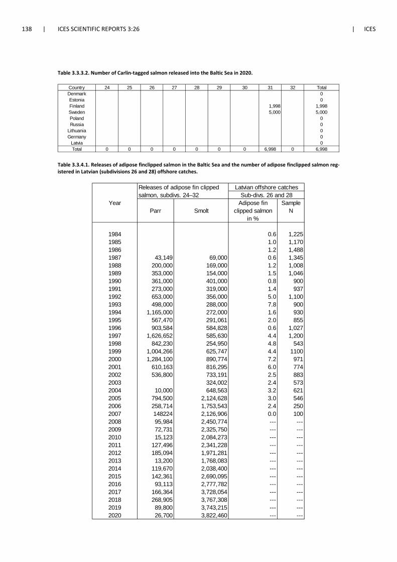
138 | ICES SCIENTIFIC REPORTS 3:26 | ICES
Table 3.3.3.2. Number of Carlin-tagged salmon released into the Baltic Sea in 2020.
Table 3.3.4.1. Releases of adipose finclipped salmon in the Baltic Sea and the number of adipose finclipped salmon reg-istered in Latvian (subdivisions 26 and 28) offshore catches.
Country 24 25 26 27 28 29 30 31 32 TotalDenmark 0Estonia 0Finland 1,998 1,998Sweden 5,000 5,000Poland 0Russia 0
Lithuania 0Germany 0
Latvia 0Total 0 0 0 0 0 0 0 6,998 0 6,998
Releases of adipose fin clipped Latvian offshore catchessalmon, subdivs. 24–32 Sub-divs. 26 and 28
Year Adipose fin SampleParr Smolt clipped salmon N
in %
1984 0.6 1,2251985 1.0 1,1701986 1.2 1,4881987 43,149 69,000 0.6 1,3451988 200,000 169,000 1.2 1,0081989 353,000 154,000 1.5 1,0461990 361,000 401,000 0.8 9001991 273,000 319,000 1.4 9371992 653,000 356,000 5.0 1,1001993 498,000 288,000 7.8 9001994 1,165,000 272,000 1.6 9301995 567,470 291,061 2.0 8551996 903,584 584,828 0.6 1,0271997 1,626,652 585,630 4.4 1,2001998 842,230 254,950 4.8 5431999 1,004,266 625,747 4.4 11002000 1,284,100 890,774 7.2 9712001 610,163 816,295 6.0 7742002 536,800 733,191 2.5 8832003 324,002 2.4 5732004 10,000 648,563 3.2 6212005 794,500 2,124,628 3.0 5462006 258,714 1,753,543 2.4 2502007 148224 2,126,906 0.0 1002008 95,984 2,450,774 --- ---2009 72,731 2,325,750 --- ---2010 15,123 2,084,273 --- ---2011 127,496 2,341,228 --- ---2012 185,094 1,971,281 --- ---2013 13,200 1,768,083 --- ---2014 119,670 2,038,400 --- ---2015 142,361 2,690,095 --- ---2016 93,113 2,777,782 --- ---2017 166,364 3,728,054 --- ---2018 268,905 3,767,308 --- ---2019 89,800 3,743,215 --- ---2020 26,700 3,822,460 --- ---
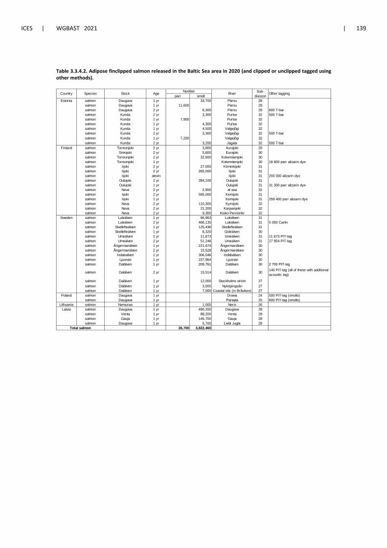
ICES | WGBAST 2021 | 139
Table 3.3.4.2. Adipose finclipped salmon released in the Baltic Sea area in 2020 (and clipped or unclipped tagged using other methods).
Sub-parr smolt division
Estonia salmon Daugava 1 yr 33,700 Pärnu 28salmon Daugava 1 yr 11,600 Pärnu 28salmon Daugava 2 yr 6,300 Pärnu 28 600 T-barsalmon Kunda 2 yr 3,300 Purtse 32 500 T-barsalmon Kunda 1 yr 7,900 Purtse 32salmon Kunda 1 yr 4,300 Purtse 32salmon Kunda 1 yr 4,500 Valgejõgi 32salmon Kunda 2 yr 3,300 Valgejõgi 32 500 T-barsalmon Kunda 1 yr 7,200 Valgejõgi 32salmon Kunda 2 yr 3,200 Jägala 32 500 T-bar
Finland salmon Tornionjoki 2 yr 3,800 Aurajoki 29salmon Simojoki 2 yr 5,600 Eurajoki 30salmon Tornionjoki 2 yr 32,600 Kokemäenjoki 30salmon Tornionjoki 1 yr Kokemäenjoki 30 18 800 parr alizarin dyesalmon Iijoki 2 yr 27,000 Kiiminkijoki 31salmon Iijoki 2 yr 265,000 Iijoki 31salmon Iijoki alevin Iijoki 31 200 000 alizarin dyesalmon Oulujoki 2 yr 284,100 Oulujoki 31salmon Oulujoki 1 yr Oulujoki 31 31 300 parr alizarin dye salmon Neva 2 yr 2,900 at sea 32salmon Iijoki 2 yr 595,000 Kemijoki 31salmon Iijoki 1 yr Kemijoki 31 259 400 parr alizarin dyesalmon Neva 2 yr 110,300 Kymijoki 32salmon Neva 2 yr 21,200 Karjaanjoki 32salmon Neva 2 yr 9,300 Kisko-Perniönki 32
Sweden salmon Luleälven 1 yr 66,963 Luleälven 31salmon Luleälven 2 yr 466,135 Luleälven 31 5 000 Carlinsalmon Skellefteälven 1 yr 125,436 Skellefteälven 31salmon Skellefteälven 1 yr 6,320 Gideälven 30salmon Umeälven 1 yr 11,673 Umeälven 31 11 673 PIT-tagsalmon Umeälven 2 yr 51,246 Umeälven 31 27 954 PIT-tagsalmon Ångermanälven 1 yr 221,674 Ångermanälven 30salmon Ångermanälven 2 yr 15,528 Ångermanälven 30salmon Indalsälven 1 yr 306,046 Indalsälven 30salmon Ljusnan 1 yr 157,964 Ljusnan 30salmon Dalälven 1 yr 209,761 Dalälven 30 2 700 PIT-tag
salmon Dalälven 2 yr 15,514 Dalälven 30 140 PIT-tag (all of these with additional acoustic tag)
salmon Dalälven 1 yr 12,000 Stockholms ström 27salmon Dalälven 1 yr 3,000 Nyköpingsån 27salmon Dalälven 1 yr 7,000 Coastal site (in Bråviken) 27
Poland salmon Daugava 1 yr Drawa 24 500 PIT-tag (smolts)salmon Daugava 1 yr Parsęta 25 600 PIT-tag (smolts)
Lithuania salmon Nemunas 1 yr 1,000 Neris 26Latvia salmon Daugava 1 yr 490,200 Daugava 28
salmon Venta 1 yr 88,200 Venta 28salmon Gauja 1 yr 145,700 Gauja 28salmon Daugava 1 yr 5,700 Lielā Jugla 28
26,700 3,822,460
Other taggingRiver
Total salmon
NumberStockSpeciesCountry Age
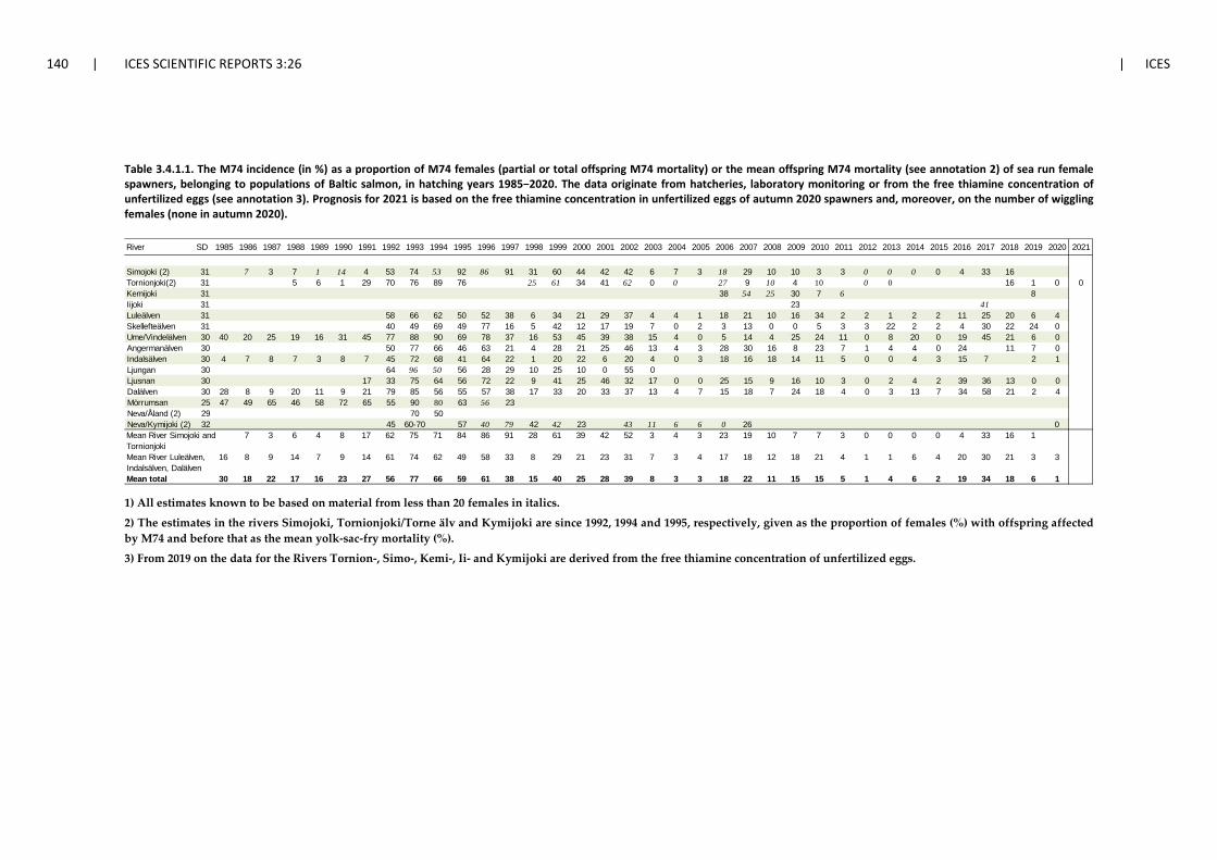
140 | ICES SCIENTIFIC REPORTS 3:26 | ICES
Table 3.4.1.1. The M74 incidence (in %) as a proportion of M74 females (partial or total offspring M74 mortality) or the mean offspring M74 mortality (see annotation 2) of sea run female spawners, belonging to populations of Baltic salmon, in hatching years 1985−2020. The data originate from hatcheries, laboratory monitoring or from the free thiamine concentration of unfertilized eggs (see annotation 3). Prognosis for 2021 is based on the free thiamine concentration in unfertilized eggs of autumn 2020 spawners and, moreover, on the number of wiggling females (none in autumn 2020).
1) All estimates known to be based on material from less than 20 females in italics.
2) The estimates in the rivers Simojoki, Tornionjoki/Torne älv and Kymijoki are since 1992, 1994 and 1995, respectively, given as the proportion of females (%) with offspring affected by M74 and before that as the mean yolk-sac-fry mortality (%).
3) From 2019 on the data for the Rivers Tornion-, Simo-, Kemi-, Ii- and Kymijoki are derived from the free thiamine concentration of unfertilized eggs.
River SD 1985 1986 1987 1988 1989 1990 1991 1992 1993 1994 1995 1996 1997 1998 1999 2000 2001 2002 2003 2004 2005 2006 2007 2008 2009 2010 2011 2012 2013 2014 2015 2016 2017 2018 2019 2020 2021
Simojoki (2) 31 7 3 7 1 14 4 53 74 53 92 86 91 31 60 44 42 42 6 7 3 18 29 10 10 3 3 0 0 0 0 4 33 16Tornionjoki(2) 31 5 6 1 29 70 76 89 76 25 61 34 41 62 0 0 27 9 10 4 10 0 0 16 1 0 0Kemijoki 31 38 54 25 30 7 6 8Iijoki 31 23 41Luleälven 31 58 66 62 50 52 38 6 34 21 29 37 4 4 1 18 21 10 16 34 2 2 1 2 2 11 25 20 6 4Skellefteälven 31 40 49 69 49 77 16 5 42 12 17 19 7 0 2 3 13 0 0 5 3 3 22 2 2 4 30 22 24 0Ume/Vindelälven 30 40 20 25 19 16 31 45 77 88 90 69 78 37 16 53 45 39 38 15 4 0 5 14 4 25 24 11 0 8 20 0 19 45 21 6 0Angermanälven 30 50 77 66 46 63 21 4 28 21 25 46 13 4 3 28 30 16 8 23 7 1 4 4 0 24 11 7 0Indalsälven 30 4 7 8 7 3 8 7 45 72 68 41 64 22 1 20 22 6 20 4 0 3 18 16 18 14 11 5 0 0 4 3 15 7 2 1Ljungan 30 64 96 50 56 28 29 10 25 10 0 55 0Ljusnan 30 17 33 75 64 56 72 22 9 41 25 46 32 17 0 0 25 15 9 16 10 3 0 2 4 2 39 36 13 0 0Dalälven 30 28 8 9 20 11 9 21 79 85 56 55 57 38 17 33 20 33 37 13 4 7 15 18 7 24 18 4 0 3 13 7 34 58 21 2 4Mörrumsan 25 47 49 65 46 58 72 65 55 90 80 63 56 23Neva/Åland (2) 29 70 50Neva/Kymijoki (2) 32 45 60-70 57 40 79 42 42 23 43 11 6 6 0 26 0Mean River Simojoki and 7 3 6 4 8 17 62 75 71 84 86 91 28 61 39 42 52 3 4 3 23 19 10 7 7 3 0 0 0 0 4 33 16 1TornionjokiMean River Luleälven, 16 8 9 14 7 9 14 61 74 62 49 58 33 8 29 21 23 31 7 3 4 17 18 12 18 21 4 1 1 6 4 20 30 21 3 3Indalsälven, DalälvenMean total 30 18 22 17 16 23 27 56 77 66 59 61 38 15 40 25 28 39 8 3 3 18 22 11 15 15 5 1 4 6 2 19 34 18 6 1
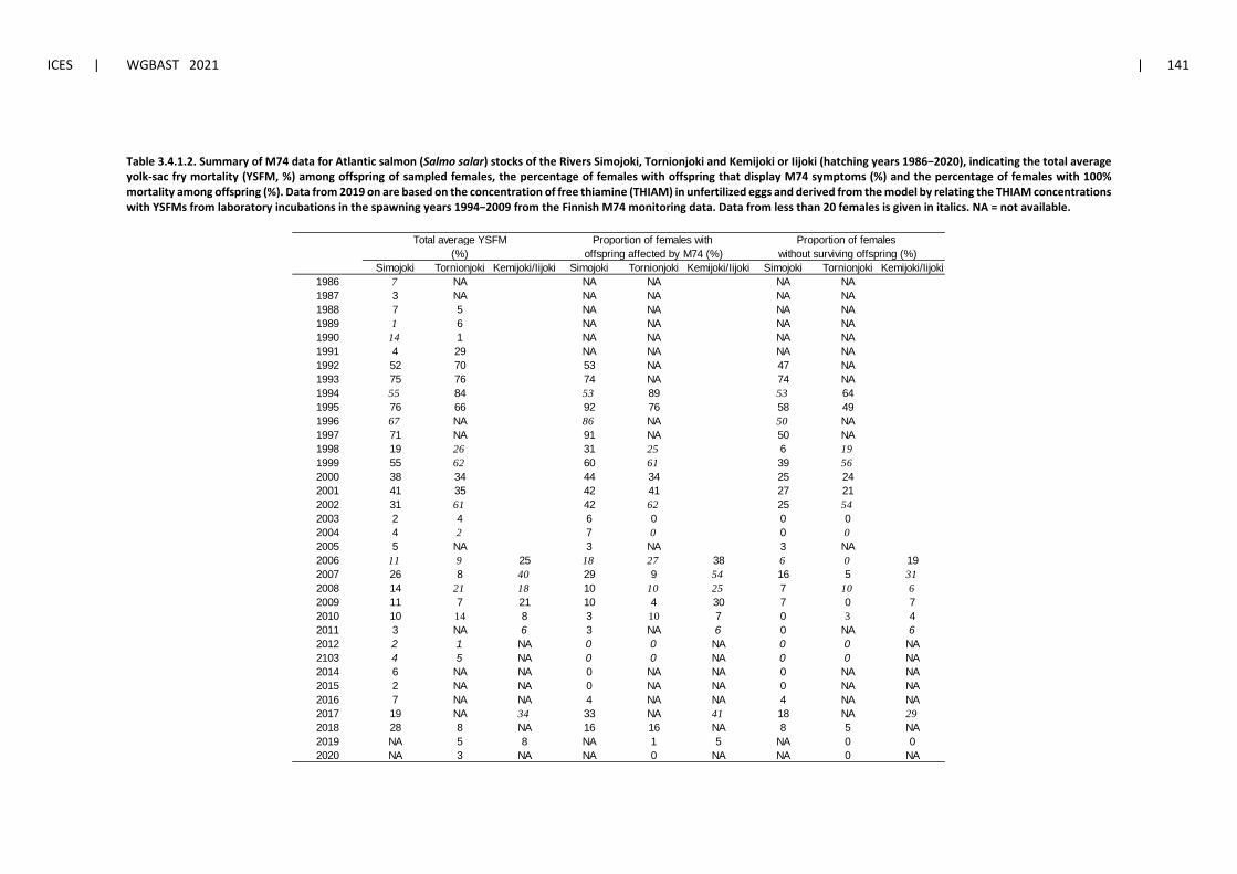
ICES | WGBAST 2021 | 141
Table 3.4.1.2. Summary of M74 data for Atlantic salmon (Salmo salar) stocks of the Rivers Simojoki, Tornionjoki and Kemijoki or Iijoki (hatching years 1986−2020), indicating the total average yolk-sac fry mortality (YSFM, %) among offspring of sampled females, the percentage of females with offspring that display M74 symptoms (%) and the percentage of females with 100% mortality among offspring (%). Data from 2019 on are based on the concentration of free thiamine (THIAM) in unfertilized eggs and derived from the model by relating the THIAM concentrations with YSFMs from laboratory incubations in the spawning years 1994−2009 from the Finnish M74 monitoring data. Data from less than 20 females is given in italics. NA = not available.
Simojoki Tornionjoki Kemijoki/Iijoki Simojoki Tornionjoki Kemijoki/Iijoki Simojoki Tornionjoki Kemijoki/Iijoki1986 7 NA NA NA NA NA1987 3 NA NA NA NA NA1988 7 5 NA NA NA NA1989 1 6 NA NA NA NA1990 14 1 NA NA NA NA1991 4 29 NA NA NA NA1992 52 70 53 NA 47 NA1993 75 76 74 NA 74 NA1994 55 84 53 89 53 641995 76 66 92 76 58 491996 67 NA 86 NA 50 NA1997 71 NA 91 NA 50 NA1998 19 26 31 25 6 191999 55 62 60 61 39 562000 38 34 44 34 25 242001 41 35 42 41 27 212002 31 61 42 62 25 542003 2 4 6 0 0 02004 4 2 7 0 0 02005 5 NA 3 NA 3 NA2006 11 9 25 18 27 38 6 0 192007 26 8 40 29 9 54 16 5 312008 14 21 18 10 10 25 7 10 62009 11 7 21 10 4 30 7 0 72010 10 14 8 3 10 7 0 3 42011 3 NA 6 3 NA 6 0 NA 62012 2 1 NA 0 0 NA 0 0 NA2103 4 5 NA 0 0 NA 0 0 NA2014 6 NA NA 0 NA NA 0 NA NA2015 2 NA NA 0 NA NA 0 NA NA2016 7 NA NA 4 NA NA 4 NA NA2017 19 NA 34 33 NA 41 18 NA 292018 28 8 NA 16 16 NA 8 5 NA2019 NA 5 8 NA 1 5 NA 0 02020 NA 3 NA NA 0 NA NA 0 NA
offspring affected by M74 (%)(%) without surviving offspring (%)Proportion of females with Total average YSFM Proportion of females
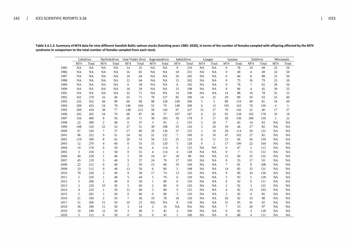
142 | ICES SCIENTIFIC REPORTS 3:26 | ICES
Table 3.4.1.3. Summary of M74 data for nine different Swedish Baltic salmon stocks (hatching years 1985−2020), in terms of the number of females sampled with offspring affected by the M74 syndrome in comparison to the total number of females sampled from each stock.
M74 Total M74 Total M74 Total M74 Total M74 Total M74 Total M74 Total M74 Total M74 Total1985 NA NA NA NA 14 35 NA NA 9 219 NA NA 0 78 19 69 23 501986 NA NA NA NA 16 82 NA NA 18 251 NA NA 0 49 4 49 24 501987 NA NA NA NA 16 64 NA NA 20 245 NA NA 0 84 8 88 32 501988 NA NA NA NA 12 64 NA NA 15 202 NA NA 0 75 16 79 23 501989 NA NA NA NA 6 38 NA NA 6 192 NA NA 0 78 7 65 29 501990 NA NA NA NA 18 59 NA NA 15 198 NA NA 0 86 4 45 39 551991 NA NA NA NA 32 71 NA NA 14 196 NA NA 14 88 16 78 35 551992 161 279 16 40 55 71 78 157 85 190 14 22 29 89 50 63 33 601993 232 352 44 89 60 68 98 128 149 206 5 5 89 119 69 81 54 601994 269 435 54 78 146 164 52 79 148 208 6 12 105 163 70 126 4 51995 209 418 38 77 148 215 58 126 97 237 15 27 79 142 22 40 17 271996 202 392 54 70 68 87 36 57 107 167 6 22 92 128 102 178 10 181997 156 409 8 50 26 71 38 183 39 178 5 17 28 130 360 159 5 221998 22 389 2 48 6 37 3 81 2 155 2 20 7 82 14 83 NA NA1999 108 316 22 53 27 51 30 108 25 126 5 20 19 46 27 82 NA NA2000 67 320 7 57 27 60 29 136 27 125 1 10 29 114 36 131 NA NA2001 96 322 9 51 24 62 31 122 7 100 0 10 47 102 27 82 NA NA2002 119 300 8 42 20 53 56 122 25 123 6 11 23 60 56 150 NA NA2003 12 270 4 60 8 53 15 120 5 128 0 2 17 100 22 164 NA NA2004 10 270 0 59 2 56 4 114 0 125 NA NA 0 47 5 112 NA NA2005 3 250 1 58 0 55 4 114 4 128 NA NA 0 7 11 151 NA NA2006 40 228 1 40 2 39 19 67 18 98 NA NA 15 60 25 132 NA NA2007 45 219 5 40 5 37 24 79 17 105 NA NA 8 55 17 93 NA NA2008 22 212 0 40 2 50 13 80 19 106 NA NA 7 81 8 108 NA NA2009 33 212 0 40 13 50 6 80 5 108 NA NA 14 85 32 131 NA NA2010 78 226 2 40 9 38 17 74 13 120 NA NA 9 90 24 136 NA NA2011 5 220 1 40 5 44 5 76 6 120 NA NA 3 93 5 128 NA NA2012 5 260 1 40 0 50 1 80 0 120 NA NA 0 92 0 111 NA NA2013 2 220 10 45 5 60 2 80 0 120 NA NA 2 92 3 121 NA NA2014 4 220 1 50 12 60 3 80 5 125 NA NA 4 92 13 103 NA NA2015 5 202 1 50 0 60 0 80 3 120 NA NA 2 92 6 85 NA NA2016 21 184 2 50 7 36 19 78 18 120 NA NA 36 92 33 98 NA NA2017 51 206 15 50 10 22 NA NA 8 120 NA NA 31 85 41 92 NA NA2018 36 180 11 50 3 14 2 19 NA NA NA NA 7 53 20 97 NA NA2019 10 180 12 50 3 48 3 45 2 100 NA NA 0 92 2 118 NA NA2020 5 112 0 50 0 52 0 45 1 100 NA NA 0 80 4 111 NA NA
Luleälven Skellelteälven Ume/Vindel älven Angermanälven MörrumsånIndalsälven Ljungan Ljusnan Dalälven
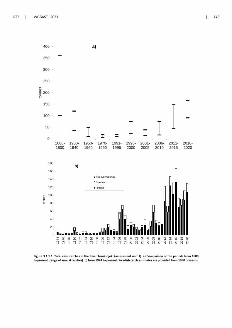
ICES | WGBAST 2021 | 143
Figure 3.1.1.1. Total river catches in the River Tornionjoki (assessment unit 1). a) Comparison of the periods from 1600 to present (range of annual catches). b) from 1974 to present. Swedish catch estimates are provided from 1980 onwards.
0
50
100
150
200
250
300
350
400
1600-1800
1900-1940
1950-1960
1970-1990
1991-1995
1996-2000
2001-2005
2006-2010
2011-2015
2016-2020
tonn
es
a)
0
20
40
60
80
100
120
140
160
180
1974
1976
1978
1980
1982
1984
1986
1988
1990
1992
1994
1996
1998
2000
2002
2004
2006
2008
2010
2012
2014
2016
2018
2020
tonn
es
Illegal/unreported
Sweden
Finland
b)
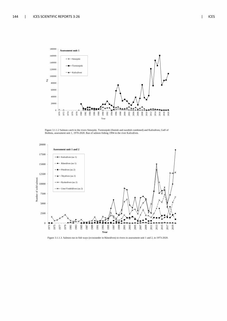
144 | ICES SCIENTIFIC REPORTS 3:26 | ICES
0
20000
40000
60000
80000
100000
120000
140000
160000
180000
1970
1972
1974
1976
1978
1980
1982
1984
1986
1988
1990
1992
1994
1996
1998
2000
2002
2004
2006
2008
2010
2012
2014
2016
2018
2020
Kg
Year
Figure 3.1.1.2 Salmon catch in the rivers Simojoki, Tornionjoki (finnish and swedish combined) and Kalixälven, Gulf of Bothnia, assessment unit 1, 1970-2020. Ban of salmon fishing 1994 in the river Kalixälven.
Simojoki
Tornionjoki
Kalixälven
Assessment unit 1
0
2500
5000
7500
10000
12500
15000
17500
20000
1973
1975
1977
1979
1981
1983
1985
1987
1989
1991
1993
1995
1997
1999
2001
2003
2005
2007
2009
2011
2013
2015
2017
2019
Year
Kalixälven (au 1)
Råneälven (au 1)
Piteälven (au 2)
Åbyälven (au 2)
Byskeälven (au 2)
Ume/Vindelälven (au 2)
Figure 3.1.1.3. Salmon run in fish ways (ecosounder in Råneälven) in rivers in assessment unit 1 and 2, in 1973-2020.
Num
ber o
f wild
salm
on
Assessment unit 1 and 2
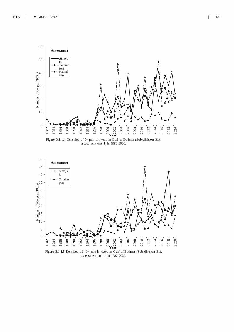
ICES | WGBAST 2021 | 145
0
10
20
30
40
50
6019
82
1984
1986
1988
1990
1992
1994
1996
1998
2000
2002
2004
2006
2008
2010
2012
2014
2016
2018
2020
YearFigure 3.1.1.4 Densities of 0+ parr in rivers in Gulf of Bothnia (Sub-division 31),
assessment unit 1, in 1982-2020.
SimojokiTornionjokiKalixälven
Assessment
Num
ber
of 0
+ pa
rr/10
0m²
0
5
10
15
20
25
30
35
40
45
50
1982
1984
1986
1988
1990
1992
1994
1996
1998
2000
2002
2004
2006
2008
2010
2012
2014
2016
2018
2020
YearFigure 3.1.1.5 Densities of >0+ parr in rivers in Gulf of Bothnia (Sub-division 31),
assessment unit 1, in 1982-2020.
SimojokiTornionjoki
Assessment
Num
ber
of >
0+ p
arr/1
00m
²
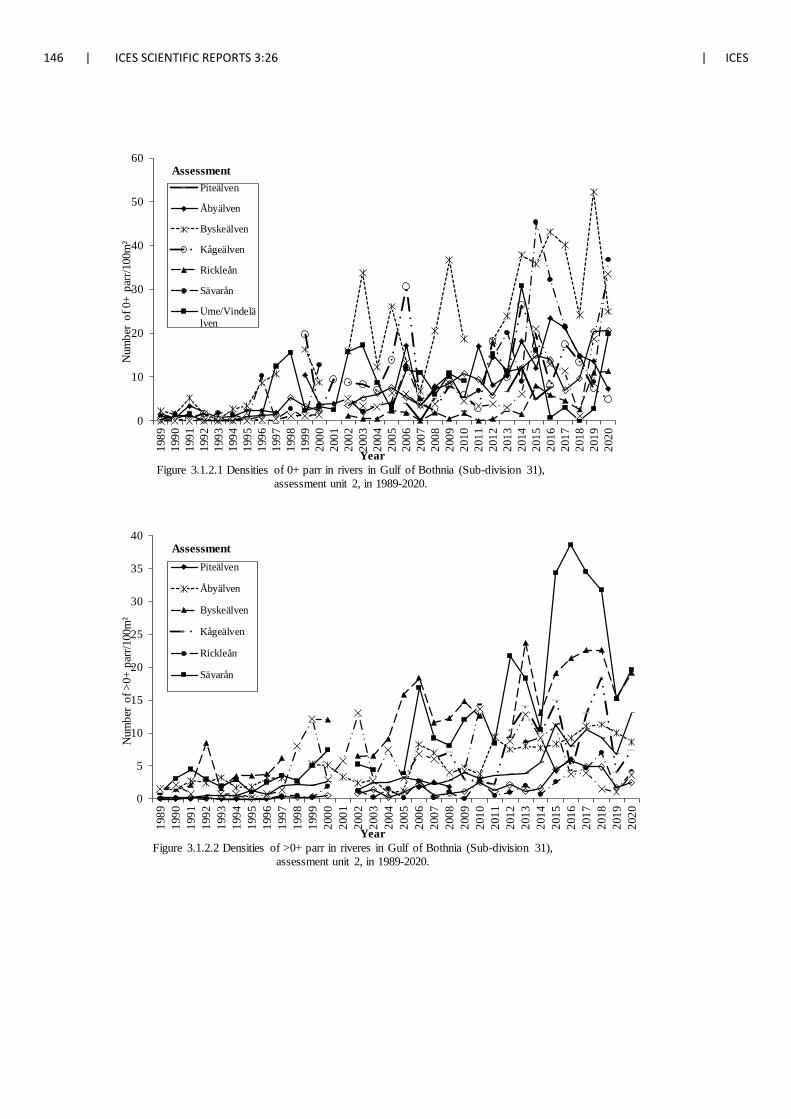
146 | ICES SCIENTIFIC REPORTS 3:26 | ICES
0
10
20
30
40
50
6019
8919
9019
9119
9219
9319
9419
9519
9619
9719
9819
9920
0020
0120
0220
0320
0420
0520
0620
0720
0820
0920
1020
1120
1220
1320
1420
1520
1620
1720
1820
1920
20
YearFigure 3.1.2.1 Densities of 0+ parr in rivers in Gulf of Bothnia (Sub-division 31),
assessment unit 2, in 1989-2020.
Piteälven
Åbyälven
Byskeälven
Kågeälven
Rickleån
Sävarån
Ume/Vindelälven
Assessment
Num
ber
of 0
+ pa
rr/10
0m²
0
5
10
15
20
25
30
35
40
1989
1990
1991
1992
1993
1994
1995
1996
1997
1998
1999
2000
2001
2002
2003
2004
2005
2006
2007
2008
2009
2010
2011
2012
2013
2014
2015
2016
2017
2018
2019
2020
YearFigure 3.1.2.2 Densities of >0+ parr in riveres in Gulf of Bothnia (Sub-division 31),
assessment unit 2, in 1989-2020.
Piteälven
Åbyälven
Byskeälven
Kågeälven
Rickleån
Sävarån
Assessment
Num
ber
of >
0+ p
arr/1
00m
²
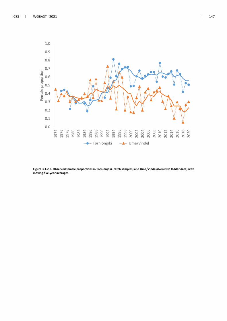
ICES | WGBAST 2021 | 147
Figure 3.1.2.3. Observed female proportions in Tornionjoki (catch samples) and Ume/Vindelälven (fish ladder data) with moving five-year averages.
0.0
0.1
0.2
0.3
0.4
0.5
0.6
0.7
0.8
0.9
1.0
1974
1976
1978
1980
1982
1984
1986
1988
1990
1992
1994
1996
1998
2000
2002
2004
2006
2008
2010
2012
2014
2016
2018
2020
Fem
ale
prop
ortio
n
Tornionjoki Ume/Vindel
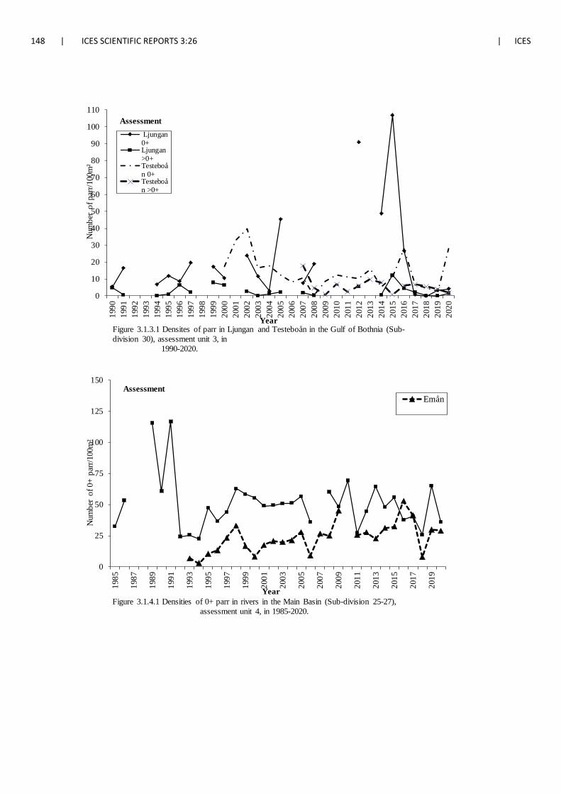
148 | ICES SCIENTIFIC REPORTS 3:26 | ICES
0
10
20
30
40
50
60
70
80
90
100
11019
9019
9119
9219
9319
9419
9519
9619
9719
9819
9920
0020
0120
0220
0320
0420
0520
0620
0720
0820
0920
1020
1120
1220
1320
1420
1520
1620
1720
1820
1920
20
YearFigure 3.1.3.1 Densites of parr in Ljungan and Testeboån in the Gulf of Bothnia (Sub-division 30), assessment unit 3, in
1990-2020.
Ljungan0+Ljungan>0+Testeboån 0+Testeboån >0+
Assessment
Num
ber
of p
arr/1
00m
²
0
25
50
75
100
125
150
1985
1987
1989
1991
1993
1995
1997
1999
2001
2003
2005
2007
2009
2011
2013
2015
2017
2019
YearFigure 3.1.4.1 Densities of 0+ parr in rivers in the Main Basin (Sub-division 25-27),
assessment unit 4, in 1985-2020.
EmånAssessment
Num
ber
of 0
+ pa
rr/10
0m²
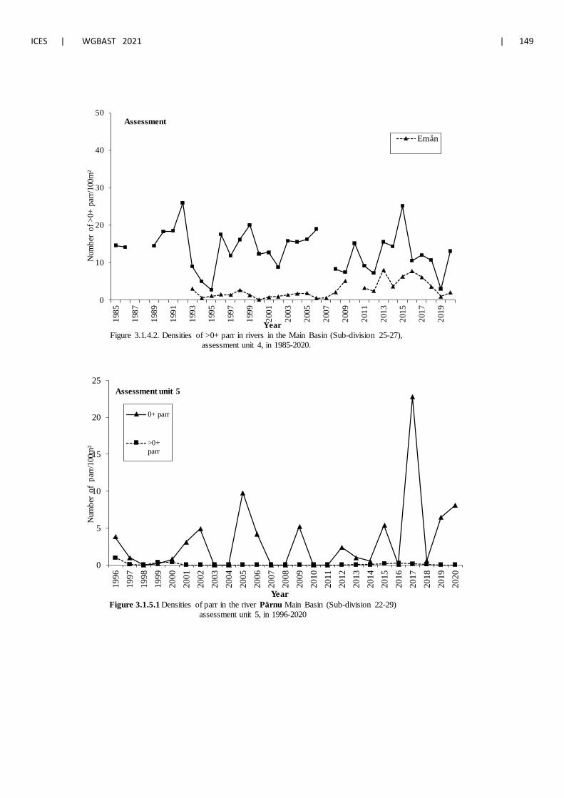
ICES | WGBAST 2021 | 149
0
10
20
30
40
5019
85
1987
1989
1991
1993
1995
1997
1999
2001
2003
2005
2007
2009
2011
2013
2015
2017
2019
YearFigure 3.1.4.2. Densities of >0+ parr in rivers in the Main Basin (Sub-division 25-27),
assessment unit 4, in 1985-2020.
Emån
Assessment
Num
ber
of >
0+ p
arr/1
00m
²
0
5
10
15
20
25
1996
1997
1998
1999
2000
2001
2002
2003
2004
2005
2006
2007
2008
2009
2010
2011
2012
2013
2014
2015
2016
2017
2018
2019
2020
YearFigure 3.1.5.1 Densities of parr in the river Pärnu Main Basin (Sub-division 22-29)
assessment unit 5, in 1996-2020
0+ parr
>0+parr
Assessment unit 5
Num
ber
of p
arr/1
00m
²
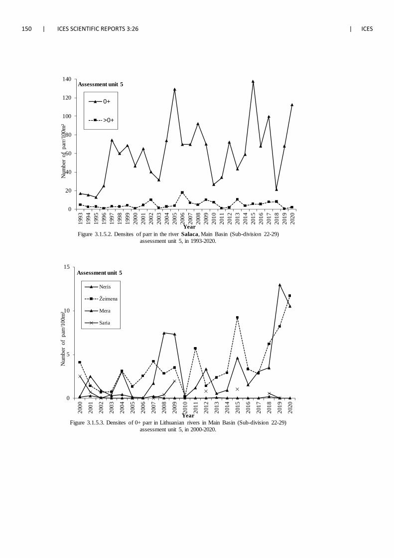
150 | ICES SCIENTIFIC REPORTS 3:26 | ICES
0
20
40
60
80
100
120
14019
9319
9419
9519
9619
9719
9819
9920
0020
0120
0220
0320
0420
0520
0620
0720
0820
0920
1020
1120
1220
1320
1420
1520
1620
1720
1820
1920
20
YearFigure 3.1.5.2. Densites of parr in the river Salaca, Main Basin (Sub-division 22-29)
assessment unit 5, in 1993-2020.
0+
>0+
Assessment unit 5
Num
ber
of p
arr/1
00m
²
0
5
10
15
2000
2001
2002
2003
2004
2005
2006
2007
2008
2009
2010
2011
2012
2013
2014
2015
2016
2017
2018
2019
2020
YearFigure 3.1.5.3. Densites of 0+ parr in Lithuanian rivers in Main Basin (Sub-division 22-29)
assessment unit 5, in 2000-2020.
Neris
Žeimena
Mera
Saria
Assessment unit 5
Num
ber
of p
arr/1
00m
²
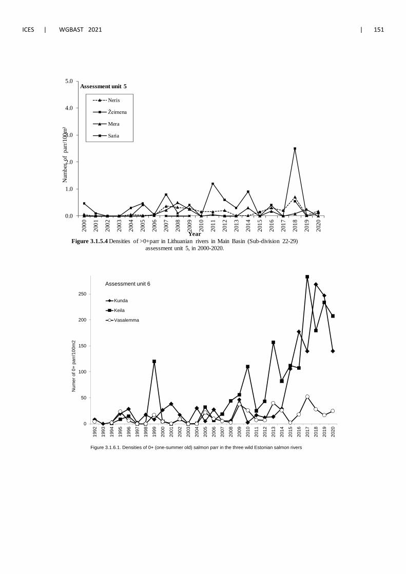
ICES | WGBAST 2021 | 151
0.0
1.0
2.0
3.0
4.0
5.020
00
2001
2002
2003
2004
2005
2006
2007
2008
2009
2010
2011
2012
2013
2014
2015
2016
2017
2018
2019
2020
YearFigure 3.1.5.4 Densities of >0+parr in Lithuanian rivers in Main Basin (Sub-division 22-29)
assessment unit 5, in 2000-2020.
Neris
Žeimena
Mera
Saria
Assessment unit 5
Num
ber
of p
arr/1
00m
²
0
50
100
150
200
250
1992
1993
1994
1995
1996
1997
1998
1999
2000
2001
2002
2003
2004
2005
2006
2007
2008
2009
2010
2011
2012
2013
2014
2015
2016
2017
2018
2019
2020
Num
er o
f 0+
parr/
100m
2
Figure 3.1.6.1. Densities of 0+ (one-summer old) salmon parr in the three wild Estonian salmon rivers
Kunda
Keila
Vasalemma
Assessment unit 6
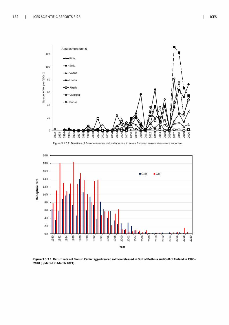
152 | ICES SCIENTIFIC REPORTS 3:26 | ICES
Figure 3.3.3.1. Return rates of Finnish Carlin tagged reared salmon released in Gulf of Bothnia and Gulf of Finland in 1980–2020 (updated in March 2021).
0
20
40
60
80
100
12019
92
1993
1994
1995
1996
1997
1998
1999
2000
2001
2002
2003
2004
2005
2006
2007
2008
2009
2010
2011
2012
2013
2014
2015
2016
2017
2018
2019
2020
Num
ber o
f 0+
parr/
100m
2
Pirita
Selja
Vääna
Loobu
Jägala
Valgejõgi
Purtse
Figure 3.1.6.2. Densities of 0+ (one-summer old) salmon parr in seven Estonian salmon rivers were suportive
Assessment unit 6
0%
2%
4%
6%
8%
10%
12%
14%
16%
18%
20%
1980
1982
1984
1986
1988
1990
1992
1994
1996
1998
2000
2002
2004
2006
2008
2010
2012
2014
2016
2018
2020
Reca
ptur
e ra
te
Year
GoB GoF
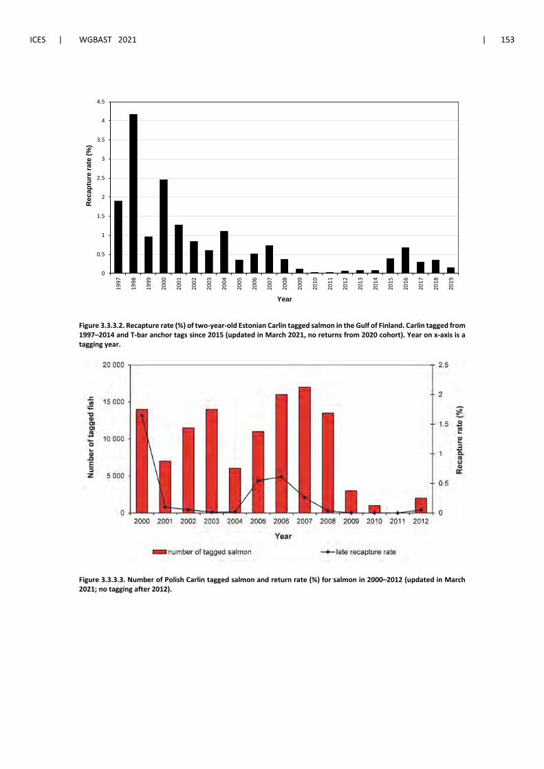
ICES | WGBAST 2021 | 153
Figure 3.3.3.2. Recapture rate (%) of two-year-old Estonian Carlin tagged salmon in the Gulf of Finland. Carlin tagged from 1997–2014 and T-bar anchor tags since 2015 (updated in March 2021, no returns from 2020 cohort). Year on x-axis is a tagging year.
Figure 3.3.3.3. Number of Polish Carlin tagged salmon and return rate (%) for salmon in 2000–2012 (updated in March 2021; no tagging after 2012).
0
0.5
1
1.5
2
2.5
3
3.5
4
4.5
1997
1998
1999
2000
2001
2002
2003
2004
2005
2006
2007
2008
2009
2010
2011
2012
2013
2014
2015
2016
2017
2018
2019
Reca
ptur
e ra
te (%
)
Year
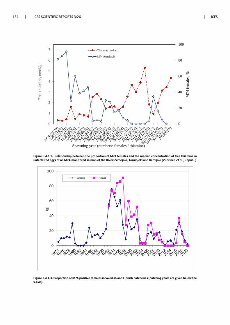
154 | ICES SCIENTIFIC REPORTS 3:26 | ICES
Figure 3.4.1.1. Relationship between the proportion of M74 females and the median concentration of free thiamine in unfertilized eggs of all M74-monitored salmon of the Rivers Simojoki, Torniojoki and Kemijoki (Vuorinen et al., unpubl.)
Figure 3.4.1.3. Proportion of M74 positive females in Swedish and Finnish hatcheries (hatching years are given below the x-axis).
0
20
40
60
80
100
0
1
2
3
4
5
6
7
M74
fem
ales
, %
Free
thia
min
e, n
mol
/g
Spawning year (numbers: females / thiamine)
Thiamine median
M74 females,%
0
20
40
60
80
100
%
Sweden Finland
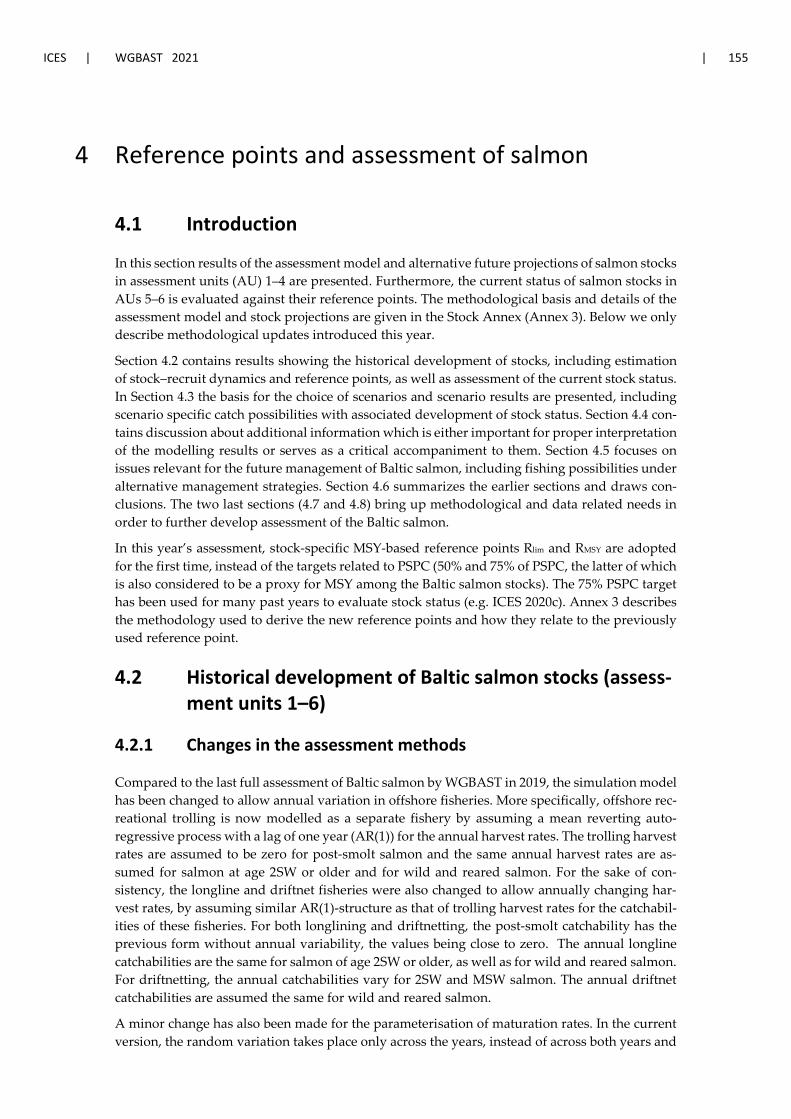
ICES | WGBAST 2021 | 155
4 Reference points and assessment of salmon
4.1 Introduction
In this section results of the assessment model and alternative future projections of salmon stocks in assessment units (AU) 1–4 are presented. Furthermore, the current status of salmon stocks in AUs 5–6 is evaluated against their reference points. The methodological basis and details of the assessment model and stock projections are given in the Stock Annex (Annex 3). Below we only describe methodological updates introduced this year.
Section 4.2 contains results showing the historical development of stocks, including estimation of stock–recruit dynamics and reference points, as well as assessment of the current stock status. In Section 4.3 the basis for the choice of scenarios and scenario results are presented, including scenario specific catch possibilities with associated development of stock status. Section 4.4 con-tains discussion about additional information which is either important for proper interpretation of the modelling results or serves as a critical accompaniment to them. Section 4.5 focuses on issues relevant for the future management of Baltic salmon, including fishing possibilities under alternative management strategies. Section 4.6 summarizes the earlier sections and draws con-clusions. The two last sections (4.7 and 4.8) bring up methodological and data related needs in order to further develop assessment of the Baltic salmon.
In this year’s assessment, stock-specific MSY-based reference points Rlim and RMSY are adopted for the first time, instead of the targets related to PSPC (50% and 75% of PSPC, the latter of which is also considered to be a proxy for MSY among the Baltic salmon stocks). The 75% PSPC target has been used for many past years to evaluate stock status (e.g. ICES 2020c). Annex 3 describes the methodology used to derive the new reference points and how they relate to the previously used reference point.
4.2 Historical development of Baltic salmon stocks (assess-ment units 1–6)
4.2.1 Changes in the assessment methods
Compared to the last full assessment of Baltic salmon by WGBAST in 2019, the simulation model has been changed to allow annual variation in offshore fisheries. More specifically, offshore rec-reational trolling is now modelled as a separate fishery by assuming a mean reverting auto-regressive process with a lag of one year (AR(1)) for the annual harvest rates. The trolling harvest rates are assumed to be zero for post-smolt salmon and the same annual harvest rates are as-sumed for salmon at age 2SW or older and for wild and reared salmon. For the sake of con-sistency, the longline and driftnet fisheries were also changed to allow annually changing har-vest rates, by assuming similar AR(1)-structure as that of trolling harvest rates for the catchabil-ities of these fisheries. For both longlining and driftnetting, the post-smolt catchability has the previous form without annual variability, the values being close to zero. The annual longline catchabilities are the same for salmon of age 2SW or older, as well as for wild and reared salmon. For driftnetting, the annual catchabilities vary for 2SW and MSW salmon. The annual driftnet catchabilities are assumed the same for wild and reared salmon.
A minor change has also been made for the parameterisation of maturation rates. In the current version, the random variation takes place only across the years, instead of across both years and
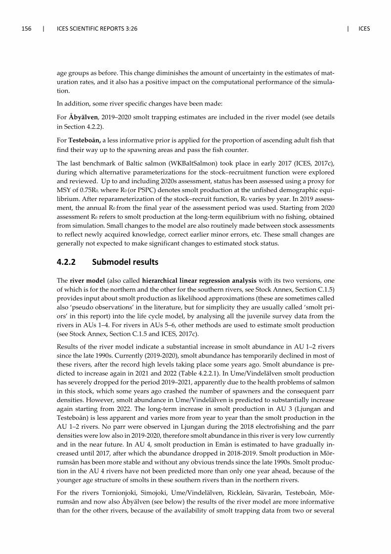
156 | ICES SCIENTIFIC REPORTS 3:26 | ICES
age groups as before. This change diminishes the amount of uncertainty in the estimates of mat-uration rates, and it also has a positive impact on the computational performance of the simula-tion.
In addition, some river specific changes have been made:
For Åbyälven, 2019–2020 smolt trapping estimates are included in the river model (see details in Section 4.2.2).
For Testeboån, a less informative prior is applied for the proportion of ascending adult fish that find their way up to the spawning areas and pass the fish counter.
The last benchmark of Baltic salmon (WKBaltSalmon) took place in early 2017 (ICES, 2017c), during which alternative parameterizations for the stock–recruitment function were explored and reviewed. Up to and including 2020s assessment, status has been assessed using a proxy for MSY of 0.75R0, where R0 (or PSPC) denotes smolt production at the unfished demographic equi-librium. After reparameterization of the stock–recruit function, R0 varies by year. In 2019 assess-ment, the annual R0 from the final year of the assessment period was used. Starting from 2020 assessment R0 refers to smolt production at the long-term equilibrium with no fishing, obtained from simulation. Small changes to the model are also routinely made between stock assessments to reflect newly acquired knowledge, correct earlier minor errors, etc. These small changes are generally not expected to make significant changes to estimated stock status.
4.2.2 Submodel results
The river model (also called hierarchical linear regression analysis with its two versions, one of which is for the northern and the other for the southern rivers, see Stock Annex, Section C.1.5) provides input about smolt production as likelihood approximations (these are sometimes called also ‘pseudo observations’ in the literature, but for simplicity they are usually called ‘smolt pri-ors’ in this report) into the life cycle model, by analysing all the juvenile survey data from the rivers in AUs 1–4. For rivers in AUs 5–6, other methods are used to estimate smolt production (see Stock Annex, Section C.1.5 and ICES, 2017c).
Results of the river model indicate a substantial increase in smolt abundance in AU 1–2 rivers since the late 1990s. Currently (2019-2020), smolt abundance has temporarily declined in most of these rivers, after the record high levels taking place some years ago. Smolt abundance is pre-dicted to increase again in 2021 and 2022 (Table 4.2.2.1). In Ume/Vindelälven smolt production has severely dropped for the period 2019–2021, apparently due to the health problems of salmon in this stock, which some years ago crashed the number of spawners and the consequent parr densities. However, smolt abundance in Ume/Vindelälven is predicted to substantially increase again starting from 2022. The long-term increase in smolt production in AU 3 (Ljungan and Testeboån) is less apparent and varies more from year to year than the smolt production in the AU 1–2 rivers. No parr were observed in Ljungan during the 2018 electrofishing and the parr densities were low also in 2019-2020, therefore smolt abundance in this river is very low currently and in the near future. In AU 4, smolt production in Emån is estimated to have gradually in-creased until 2017, after which the abundance dropped in 2018-2019. Smolt production in Mör-rumsån has been more stable and without any obvious trends since the late 1990s. Smolt produc-tion in the AU 4 rivers have not been predicted more than only one year ahead, because of the younger age structure of smolts in these southern rivers than in the northern rivers.
For the rivers Tornionjoki, Simojoki, Ume/Vindelälven, Rickleån, Sävarån, Testeboån, Mör-rumsån and now also Åbyälven (see below) the results of the river model are more informative than for the other rivers, because of the availability of smolt trapping data from two or several
ICES | WGBAST 2021 | 157
years. Also, smolt estimates of years without smolt trapping have become somewhat more pre-cise in these rivers. Smolt trapping has been conducted only in one year in Lögdeälven and Emån, which increases the precision of smolt abundance mainly in that specific year.
This year, some important modifications to the river model indata for Åbyälven (AU 2) were made. The salmon habitats in this river consist of two main sections - below and above the Hed-näs hydropower dam, located 36 km from the river mouth. The power plant was constructed in 1920, rebuilt in 1977, and equipped with a fish ladder in 1995. Earlier, salmon and sea trout could only reproduce below the dam. The amount of adult salmon passing Hednäs has increased over time (see Section 3.1.2), but the number of fish counted in the ladder is perceived low in relation to the amount of available habitat located in the upstream part of the river. The reason seems to be migration problems for ascending adults at the dam combined with very high mortality (>90%) among smolts when passing the reservoir, turbines and the fish ladder (Gustafsson, 2010).
Since the early 2000s, a total of 14 (20 since 2019) electrofishing stations have been fished annu-ally, whereof four are located above the dam. Although parr abundance in both river sections (below/above Hednäs) show positive trends, average parr densities have remained clearly higher in the downstream section (Table 3.1.2.1). Following a recent review of why results from smolt trapping 2018–2020 yielded markedly lower estimates of smolt abundance in Åbyälven compared to results from the river model (in which smolt trapping data have not been included in previous assessments), it was revealed that only the ten (16 since 2019) downstream electro-fishing stations have so far been used in the model. In contrast, spawning habitats located below and above Hednäs are included in the total river habitat that goes into the model. This may ex-plain why the river model estimates of smolt abundance for Åbyälven have been much higher than indicated by the smolt counting.
To adjust this previous mismatch, combined parr densities for the two river sections, weighted according to relative estimated habitat areas (63% below and 37% above Hednäs), were used as input data for the 2021 river model. For years before 1995, when salmon could not pass the Hed-näs power station, average parr densities for the upper section were set to zero. Before weighting, the high estimated mortality (93%) among smolts from the upper river section was accounted for by multiplying the corresponding average parr density with 0.07. In addition to updated parr densities, smolt trapping estimates from 2019 and 2020 are now included in the river model, whereas the 2018 estimate was omitted as the earliest part of the Åbyälven smolt run in that year may have been missed.
Until next year, the plan is to revisit estimated sizes of salmon habitats in Åbyälven, including the relative proportion below and above Hednäs. In addition, the prior distribution for carrying capacity (K) needs to be updated using the same approach as has recently been used for other salmon rivers. Development of a more refined method to model the high mortality for smolts when passing Hednäs would also be desirable.
A model for M74 mortality provides input about fry mortality due to M74 into the life cycle model by analysing all data on incidence of M74 in the stocks (see Stock Annex, Section C.1.6). Figure 4.2.2.1 shows the estimates for M74 mortality (median and 95% probability interval); within the last ten years, the mortality decreased until the spawning years 2015–2016 when it increased to the level of magnitude of 5–20%. The results from the spawning in 2017, 2018 and 2019 (Figure 4.2.2.1) and the predictions made for 2020 spawning (Section 3.4) show a return to the low level prevailed in the early 2010s. In general, the percentage of females with offspring affected by M74 overestimates the M74 mortality due to the fact that part of the offspring will die due to normal yolk-sac-fry mortality, unrelated to M74. Also, not all offspring necessarily die when affected by M74. Because of the decreasing trend in mortality among offspring of females affected by M74, the data on proportion of females affected by M74 especially overestimate M74 mortality in recent years. Data on the total average yolk-sac-fry mortality are much better at
158 | ICES SCIENTIFIC REPORTS 3:26 | ICES
tracking the general trend but overestimate the actual M74 mortality, because these data do not distinguish between normal yolk-sac-fry mortality and yolk-sac-fry mortality caused by the M74 syndrome. Table 4.2.2.2 shows the actual values of the M74 mortality for the different salmon stocks. Figure 4.2.2.2 illustrates the probability that offspring of M74-affected females would die, which has been possible to calculate for Simojoki, Tornionjoki and an “unsampled salmon stock”.
4.2.3 Status of the assessment unit 1–4 stocks and development of fisheries in the Gulf of Bothnia and the Main Basin
The full life-history model (FLHM) was run with two chains for 675 000 iterations after an adap-tive phase of 10 000 iterations. The first 150 000 iterations were discarded as burn-in and the chains were thinned with an interval of 350 to yield a final sample size of 3000 (1500 iterations from each of two chains). Inspection of traceplots and Gelman-Rubin diagnostics indicated poor convergence for many parameters. On closer inspection it became apparent that one of the chains (chain one) was getting stuck at implausible values for many variables. It was therefore decided to base results on only one chain for this year’s assessment as in 2019. In order to ensure that the most representative chain was selected for each parameter and variable in the model, the means from each chain were compared to posterior means from a longer converged run of 2020s assess-ment model, and the chain with the closest mean was selected for that parameter/variable. Start-ing with chain two as the default, this resulted in 9219 parameter/variables being substituted in from chain one, out of a possible 19 606 in the longer converged run. Some caution must therefore be taken in the interpretation of results. In the text and figures that follow, medians and 90% probability intervals (PI’s) are used where possible as statistics of posterior probability distribu-tions.
The results indicate a decreasing long-term trend in the post-smolt survival until mid-2000, after which survival has generally somewhat improved (Figure 4.2.3.1). The lowest overall survival was estimated for salmon that smolted in years 2005–2006 (median estimate around 8–10% among wild and 5% among reared smolts), and survival was relatively low also in 2007–2009. Low survivals were estimated for either wild or reared smolts also in some years of the last dec-ade, but the average survival in that decade was higher than in 2005–2009: 15% for wild smolts and 9% for reared smolts (median estimates ranging from 11–19% and 3–14% among wild and reared post-smolts, respectively). Survival was relatively high especially among wild salmon that smolted in 2010–2012 and 2014 (Figure 4.2.3.1). After the relatively high survival among 2017 wild smolts (16%) and poor survival among 2018 wild smolts (11%), survival is currently close to its average level (14% in 2019, which is the last smolting year with data to estimate).
The adult natural annual survival of wild salmon (median 91%, PI 86–95%) is estimated to be clearly higher than that of reared salmon (median 76%, PI 71–85%). Thus, the difference in total sea survival back to the spawning/stocking site for wild and reared salmon is large because of the survival difference both at post-smolt and at later marine stages.
Maturation (homing rate) of 1-sea winter salmon (grilse) has in most years been around 10–20% (average of medians over the whole time-series is 16%) and 20–50% (average of medians over the whole time-series is 34%) among wild and reared individuals, respectively (Figure 4.2.3.2). Differences between wild and reared salmon are smaller among multi-sea winter salmon, but in each sea age reared salmon has on average higher maturation rate. Generally, 30–60%, 60–70% and 50–70% of 2SW, 3SW and 4SW feeding salmon have matured, respectively. The estimated maturation rates of four-sea winter are on average lower than those of three-sea winter salmon. This is against intuition but might be an artefact due to the inconsistency between current model assumptions (no repeat spawners, all fish mature at latest after five sea winters) and the biology of salmon (some repeat spawners exist and some salmon have a longer lifespan than five years
ICES | WGBAST 2021 | 159
at sea). Maturation rates of reared salmon have generally increased over time, but no similar trend is visible among wild salmon. Maturation rates were generally on the lowest levels around 2010–2012.
The full life-history model allows estimation of the stock-specific stock–recruit relationships, which are presented as summary statistics (Tables 4.2.3.1 and 4.2.3.2) and graphically (Figures 4.2.1.1, 4.2.3.3 and 4.2.3.4). Table 4.2.3.2 and Figure 4.2.3.4 also show the estimates of the stock-specific reference points (Rlim and RMSY), which are used to assess stock status. “Equilibrium smolt production” corresponds to the Potential Smolt Production Capacity PSPC, i.e. the average smolt production that can be reached in the long term without fishing. It is important to note, that these PSPC estimates are not directly comparable to the PSPC estimates presented in earlier years’ assessments (e.g. ICES, 2019), where estimated PSPCs from the final year of the assessment pe-riod were used. In this year’s assessment, PSPCs from simulation are used (as in 2020), assuming reversion to long-term average vital rates (covering the whole historical time-series) for most time-varying parameters into the future. Among stocks the point values of Rlim and RMSY range from 15–40% and 60–85% of their corresponding PSPC’s point values, respectively (Table 4.2.3.2). Figure 4.2.3.3 gives an indication of river-specific stock–recruit curves. The blue clouds in the figure panels indicate posterior probability distributions of all the historical estimates of yearly egg deposition and corresponding smolt abundance (the density of the cloud indicates the prob-ability). Curves added in the figure panels are draws from the posterior distribution of the Beverton–Holt stock–recruit function. Figure 4.2.3.4 illustrates how uncertainty related to the estimates of PSPC, Rlim and RMSY vary between stocks. It is difficult to fully explain the between-stock variation in the level of uncertainty, but it is likely an outcome of several factors like stock-specific assumptions about vital rates, the amount of stock-specific data, the coherence of data and the amount of contrast existing in the data in relation to the stock size. The total combined PSPC estimate containing all the AU 1-4 stocks is about 3.1 million (median, 90% PI’s 2.5-4.1 million) smolts (Table 4.2.3.2). Of this, AU 1 stocks account for about 80%, and AU 2 stocks ac-count for about 18%. When adding the point estimates of PSPC shown in the Table 4.2.3.3 for the AU 5 (301 000 smolts) and AU 6 (273 000 smolts), which are based of expert judgments, the total combined PSPC of all the assessed Baltic Sea salmon stocks is about 3.7 million smolts.
Since the mid-1990s, the status of many wild salmon populations in the Baltic Sea has improved, and the total wild production has increased from less than 0.5 to about three million smolts (Fig-ure 4.2.3.5, Table 4.2.3.3). After the record year 2017 (with median estimate of 3.14 million smolts) the total wild production has somewhat declined and it was 2.75 million smolts (median esti-mate) in 2020. Since the mid-2010s, the total smolt production of the AU 1 stocks has been clearly above the median estimates of both the combined Rlim and RMSY of AU 1, and it has been fluctu-ating close to the median estimate of combined PSPC (R0) of these stocks. In AU 2, the combined smolt production has been fluctuating around the median estimate of the combined RMSY of AU 2 stocks. Also, in the AU 3 and AU 4 total smolt production has been recently near the median estimates of the combined RMSY of the respective AU’s. Since the mid-2010s, the total combined AU 1–4 smolt production has been fluctuating between the median estimates of the total com-bined Rlim and RMSY of all these AUs (Figure 4.2.3.5).
There are regional differences in trends in smolt production. For the wild salmon stocks of AUs 1–2, the very fast recovery of smolt production indicates high steepness for stock–recruit rela-tionships in these rivers. The recovery is most pronounced in the largest rivers, but recently the salmon stocks spawning in smaller ‘forest rivers’ of the region (Åbyälven, Rickleån, Sävarån, Öreälven, Lögdeälven) have speeded up their recovery. However, their stock status (current pro-duction level against MSY) is assessed to be lower than that of the larger salmon rivers, as dis-cussed below. The two wild stocks in AU 3 have also recovered, but the estimates of the current and/or the potential smolt production of Ljungan and Testeboån are highly uncertain. In AU 4
160 | ICES SCIENTIFIC REPORTS 3:26 | ICES
the Mörrumsån stock has stayed relatively stable, while the abundance in Emån has been grad-ually increasing. The AU 5 stocks are characterized by large interannual variation in smolt pro-duction and varying trends in the production. Smolt production in the Nemunas river system has been increasing especially in the latest years, while in Salaca and Gauja the production has been fluctuation without clear trends. Smolt production in Venta shows a decreasing trend. Many AU 5 rivers are very small and their estimated PSPC is in some thousands of smolts only; the existing data from these rivers are fragmentary and typically indicate zero or near-zero an-nual smolt production (see more details in Section 4.2.4).
By comparing the final year (2020) posterior smolt production (Table 4.2.3.3) against the esti-mated reference points Rlim and RMSY, it is possible to evaluate the current status of the AU 1–4 stocks in terms of their probability to reach the reference points (Table 4.2.3.4a). Table 4.2.3.4b contains wild and mixed AU 5–6 stocks, which are currently not included in the FLHM. These stocks have not been analytically derived, but expert judgments are used to classify their current status in relation to their PSPC. Because the estimates of annual smolt production vary greatly among AU 5–6 stocks (partly an artefact caused by assuming that all smolts are 2-year olds), the current status assessment is calculated in two ways: 1) by using only the 2020 smolt production estimate, and 2) by using the average of the 2018–2020 smolt production estimates.
Out of the 17 assessed stocks in AU 1–4, nine have reached Rlim with >95% probability, three stocks have reached Rlim with 70–95% probability, two stocks have reached Rlim with 50–70% probability, and three stocks have reached Rlim with <50% probability (Table 4.2.3.4a). All stocks in the AU 1 are estimated to have reached their Rlim with 99–100% probability, and the corre-sponding probabilities of having reached their RMSY vary between 60–80%. In AU 2, three stocks (Piteälven, Byskeälven and Vindelälven) have reached their Rlim with >95% probability, while among the rest of the AU 2 rivers the corresponding probabilities range from 40% (Lögdeälven) to 89% (Sävarån). The probabilities for having reached RMSY vary between 9% (Rickleån and Lö-gdeälven) and 77% (Piteälven). In AU 3, Ljungan has a low probability (< 40%) of having reached either of the reference points, while Testeboån has likely (with >70% probability) reached both reference points. A similar divided status prevails among the AU 4 stocks, where Mörrumsån has likely reached both Rlim (100% probability) and RMSY (76% probability), whereas Emån has unlikely reached either of them (28% and 9% corresponding probabilities). As discussed in Sec-tion 4.4.2, current stock status of Piteälven (AU 2) and Testeboån (AU 3) is most likely overesti-mated.
Among the twelve AU 5 stocks, the wild Salaca (2020 and 2018–2010 average smolt production is 43% and 40% of PSPC, respectively) and mixed Nemunas (2020 and 2018–2010 average smolt production is 32% and 21% of PSPC, respectively) stocks have the highest current status. Among the remaining wild and mixed AU 5 stocks, current smolt production is <10% of the respective PSPC (Table 4.2.3.4b).
A large majority of the twelve AU 6 stocks has reached a higher proportion of their PSPC than the AU 5 stocks. Smolt production in the Kunda stock has reached 100% of its PSPC, and the production in the Keila stock is also very high (2020 and 2018–2010 average smolt production is 88% and 96% of PSPC, respectively). The current smolt production is <10% of the PSPC in the mixed stocks of Luga, Valgejögi, Jägala and Vääna (Table 4.2.3.4b).
The full life-history model (FLHM) captures quite well the overall historic fluctuation of catches in various fisheries, especially from the last ten years (Figure 4.2.3.6). However, catches from the first decade of this millennium tend to become underestimated for most of the years and fisher-ies. The model also does not fully capture the high river catches of the years 2008–2009 (Figure 4.2.3.6).
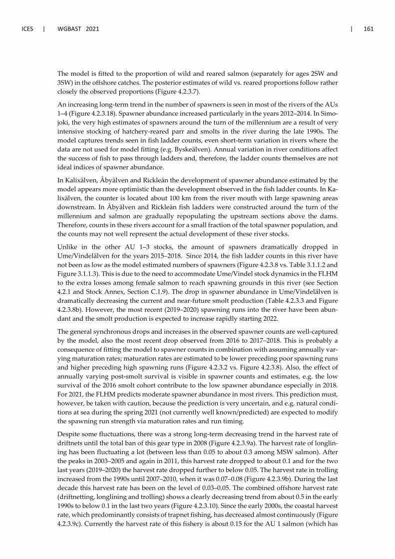
ICES | WGBAST 2021 | 161
The model is fitted to the proportion of wild and reared salmon (separately for ages 2SW and 3SW) in the offshore catches. The posterior estimates of wild vs. reared proportions follow rather closely the observed proportions (Figure 4.2.3.7).
An increasing long-term trend in the number of spawners is seen in most of the rivers of the AUs 1–4 (Figure 4.2.3.18). Spawner abundance increased particularly in the years 2012–2014. In Simo-joki, the very high estimates of spawners around the turn of the millennium are a result of very intensive stocking of hatchery-reared parr and smolts in the river during the late 1990s. The model captures trends seen in fish ladder counts, even short-term variation in rivers where the data are not used for model fitting (e.g. Byskeälven). Annual variation in river conditions affect the success of fish to pass through ladders and, therefore, the ladder counts themselves are not ideal indices of spawner abundance.
In Kalixälven, Åbyälven and Rickleån the development of spawner abundance estimated by the model appears more optimistic than the development observed in the fish ladder counts. In Ka-lixälven, the counter is located about 100 km from the river mouth with large spawning areas downstream. In Åbyälven and Rickleån fish ladders were constructed around the turn of the millennium and salmon are gradually repopulating the upstream sections above the dams. Therefore, counts in these rivers account for a small fraction of the total spawner population, and the counts may not well represent the actual development of these river stocks.
Unlike in the other AU 1–3 stocks, the amount of spawners dramatically dropped in Ume/Vindelälven for the years 2015–2018. Since 2014, the fish ladder counts in this river have not been as low as the model estimated numbers of spawners (Figure 4.2.3.8 vs. Table 3.1.1.2 and Figure 3.1.1.3). This is due to the need to accommodate Ume/Vindel stock dynamics in the FLHM to the extra losses among female salmon to reach spawning grounds in this river (see Section 4.2.1 and Stock Annex, Section C.1.9). The drop in spawner abundance in Ume/Vindelälven is dramatically decreasing the current and near-future smolt production (Table 4.2.3.3 and Figure 4.2.3.8b). However, the most recent (2019–2020) spawning runs into the river have been abun-dant and the smolt production is expected to increase rapidly starting 2022.
The general synchronous drops and increases in the observed spawner counts are well-captured by the model, also the most recent drop observed from 2016 to 2017–2018. This is probably a consequence of fitting the model to spawner counts in combination with assuming annually var-ying maturation rates; maturation rates are estimated to be lower preceding poor spawning runs and higher preceding high spawning runs (Figure 4.2.3.2 vs. Figure 4.2.3.8). Also, the effect of annually varying post-smolt survival is visible in spawner counts and estimates, e.g. the low survival of the 2016 smolt cohort contribute to the low spawner abundance especially in 2018. For 2021, the FLHM predicts moderate spawner abundance in most rivers. This prediction must, however, be taken with caution, because the prediction is very uncertain, and e.g. natural condi-tions at sea during the spring 2021 (not currently well known/predicted) are expected to modify the spawning run strength via maturation rates and run timing.
Despite some fluctuations, there was a strong long-term decreasing trend in the harvest rate of driftnets until the total ban of this gear type in 2008 (Figure 4.2.3.9a). The harvest rate of longlin-ing has been fluctuating a lot (between less than 0.05 to about 0.3 among MSW salmon). After the peaks in 2003–2005 and again in 2011, this harvest rate dropped to about 0.1 and for the two last years (2019–2020) the harvest rate dropped further to below 0.05. The harvest rate in trolling increased from the 1990s until 2007–2010, when it was 0.07–0.08 (Figure 4.2.3.9b). During the last decade this harvest rate has been on the level of 0.03–0.05. The combined offshore harvest rate (driftnetting, longlining and trolling) shows a clearly decreasing trend from about 0.5 in the early 1990s to below 0.1 in the last two years (Figure 4.2.3.10). Since the early 2000s, the coastal harvest rate, which predominantly consists of trapnet fishing, has decreased almost continuously (Figure 4.2.3.9c). Currently the harvest rate of this fishery is about 0.15 for the AU 1 salmon (which has
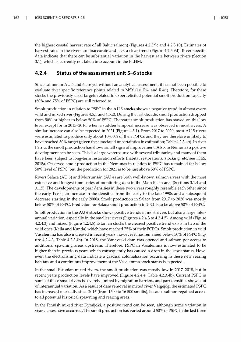
162 | ICES SCIENTIFIC REPORTS 3:26 | ICES
the highest coastal harvest rate of all Baltic salmon) (Figures 4.2.3.9c and 4.2.3.10). Estimates of harvest rates in the rivers are inaccurate and lack a clear trend (Figure 4.2.3.9d). River-specific data indicate that there can be substantial variation in the harvest rate between rivers (Section 3.1), which is currently not taken into account in the FLHM.
4.2.4 Status of the assessment unit 5–6 stocks
Since salmon in AU 5 and 6 are yet without an analytical assessment, it has not been possible to evaluate river specific reference points related to MSY (i.e. Rlim and RMSY). Therefore, for these stocks the previously used targets related to expert elicited potential smolt production capacity (50% and 75% of PSPC) are still referred to.
Smolt production in relation to PSPC in the AU 5 stocks shows a negative trend in almost every wild and mixed river (Figures 4.5.1 and 4.5.2). During the last decade, smolt production dropped from 50% or higher to below 50% of PSPC. Thereafter smolt production has stayed on this low level except for in 2015–2016, when a sudden temporal increase was observed in most rivers. A similar increase can also be expected in 2021 (Figure 4.5.1). From 2017 to 2020, most AU 5 rivers were estimated to produce only about 10–30% of their PSPCs and they are therefore unlikely to have reached 50% target (given the associated uncertainties in estimation; Table 4.2.3.4b). In river Pärnu, the smolt production has shown small signs of improvement. Also, in Nemunas a positive development can be seen. This is a large watercourse with several tributaries, and many of them have been subject to long-term restoration efforts (habitat restorations, stocking, etc. see ICES, 2018a. Observed smolt production in the Nemunas in relation to PSPC has remained far below 50% level of PSPC, but the prediction for 2021 is to be just above 50% of PSPC.
Rivers Salaca (AU 5) and Mörrumsån (AU 4) are both well-known salmon rivers with the most extensive and longest time-series of monitoring data in the Main Basin area (Sections 3.1.4 and 3.1.5). The developments of parr densities in these two rivers roughly resemble each other since the early 1990s; an increase in the densities from the early to the late 1990s and a subsequent decrease starting in the early 2000s. Smolt production in Salaca from 2017 to 2020 was mostly below 50% of PSPC. Prediction for Salaca smolt production in 2021 is to be above 50% of PSPC.
Smolt production in the AU 6 stocks shows positive trends in most rivers but also a large inter-annual variation, especially in the smallest rivers (Figures 4.2.4.3 to 4.2.4.5). Among wild (Figure 4.2.4.3) and mixed (Figure 4.2.4.5) Estonian stocks the clearest positive trend exists in two of the wild ones (Keila and Kunda) which have reached 75% of their PCPCs. Smolt production in wild Vasalemma has also increased in recent years, however it has remained below 50% of PSPC (Fig-ure 4.2.4.3, Table 4.2.3.4b). In 2018, the Vanaveski dam was opened and salmon got access to additional spawning areas upstream. Therefore, PSPC in Vasalemma is now estimated to be higher than in previous years which consequently has caused a drop in the stock status. How-ever, the electrofishing data indicate a gradual colonialization occurring in these new rearing habitats and a continuous improvement of the Vasalemma stock status is expected.
In the small Estonian mixed rivers, the smolt production was mostly low in 2017–2018, but in recent years production levels have improved (Figure 4.2.4.4, Table 4.2.3.4b). Current PSPC in some of these small rivers is severely limited by migration barriers, and parr densities show a lot of interannual variation. As a result of dam removal in mixed river Valgejõgi the estimated PSPC has increased markedly since 2016 (from 1500 to 16 500 smolts), because salmon regained access to all potential historical spawning and rearing areas.
In the Finnish mixed river Kymijoki, a positive trend can be seen, although some variation in year classes have occurred. The smolt production has varied around 50% of PSPC in the last three
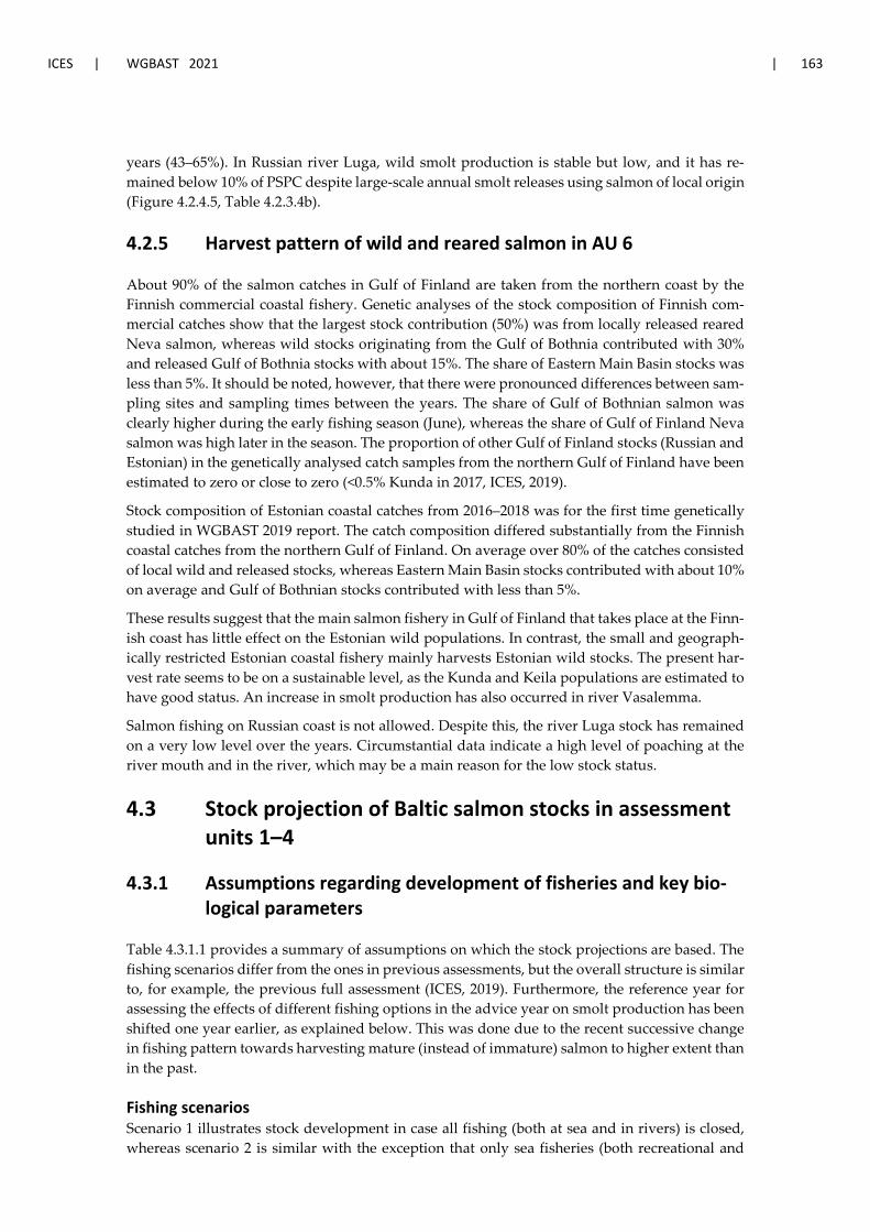
ICES | WGBAST 2021 | 163
years (43–65%). In Russian river Luga, wild smolt production is stable but low, and it has re-mained below 10% of PSPC despite large-scale annual smolt releases using salmon of local origin (Figure 4.2.4.5, Table 4.2.3.4b).
4.2.5 Harvest pattern of wild and reared salmon in AU 6
About 90% of the salmon catches in Gulf of Finland are taken from the northern coast by the Finnish commercial coastal fishery. Genetic analyses of the stock composition of Finnish com-mercial catches show that the largest stock contribution (50%) was from locally released reared Neva salmon, whereas wild stocks originating from the Gulf of Bothnia contributed with 30% and released Gulf of Bothnia stocks with about 15%. The share of Eastern Main Basin stocks was less than 5%. It should be noted, however, that there were pronounced differences between sam-pling sites and sampling times between the years. The share of Gulf of Bothnian salmon was clearly higher during the early fishing season (June), whereas the share of Gulf of Finland Neva salmon was high later in the season. The proportion of other Gulf of Finland stocks (Russian and Estonian) in the genetically analysed catch samples from the northern Gulf of Finland have been estimated to zero or close to zero (<0.5% Kunda in 2017, ICES, 2019).
Stock composition of Estonian coastal catches from 2016–2018 was for the first time genetically studied in WGBAST 2019 report. The catch composition differed substantially from the Finnish coastal catches from the northern Gulf of Finland. On average over 80% of the catches consisted of local wild and released stocks, whereas Eastern Main Basin stocks contributed with about 10% on average and Gulf of Bothnian stocks contributed with less than 5%.
These results suggest that the main salmon fishery in Gulf of Finland that takes place at the Finn-ish coast has little effect on the Estonian wild populations. In contrast, the small and geograph-ically restricted Estonian coastal fishery mainly harvests Estonian wild stocks. The present har-vest rate seems to be on a sustainable level, as the Kunda and Keila populations are estimated to have good status. An increase in smolt production has also occurred in river Vasalemma.
Salmon fishing on Russian coast is not allowed. Despite this, the river Luga stock has remained on a very low level over the years. Circumstantial data indicate a high level of poaching at the river mouth and in the river, which may be a main reason for the low stock status.
4.3 Stock projection of Baltic salmon stocks in assessment units 1–4
4.3.1 Assumptions regarding development of fisheries and key bio-logical parameters
Table 4.3.1.1 provides a summary of assumptions on which the stock projections are based. The fishing scenarios differ from the ones in previous assessments, but the overall structure is similar to, for example, the previous full assessment (ICES, 2019). Furthermore, the reference year for assessing the effects of different fishing options in the advice year on smolt production has been shifted one year earlier, as explained below. This was done due to the recent successive change in fishing pattern towards harvesting mature (instead of immature) salmon to higher extent than in the past.
Fishing scenarios Scenario 1 illustrates stock development in case all fishing (both at sea and in rivers) is closed, whereas scenario 2 is similar with the exception that only sea fisheries (both recreational and
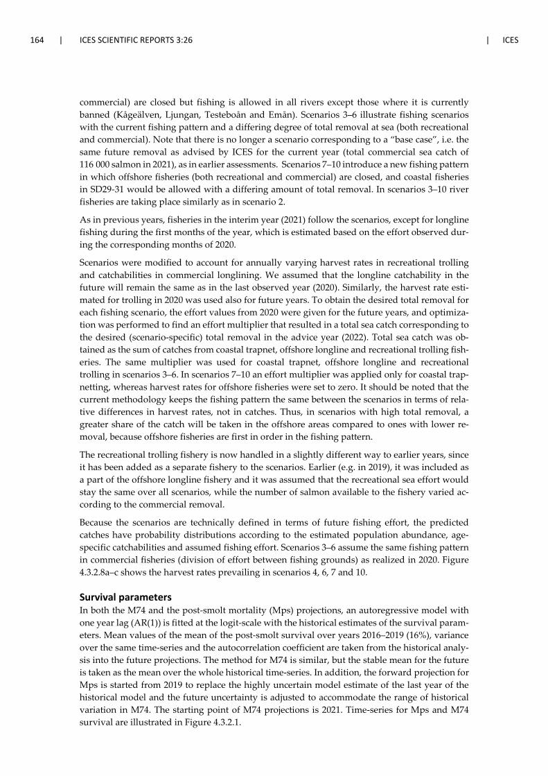
164 | ICES SCIENTIFIC REPORTS 3:26 | ICES
commercial) are closed but fishing is allowed in all rivers except those where it is currently banned (Kågeälven, Ljungan, Testeboån and Emån). Scenarios 3–6 illustrate fishing scenarios with the current fishing pattern and a differing degree of total removal at sea (both recreational and commercial). Note that there is no longer a scenario corresponding to a “base case”, i.e. the same future removal as advised by ICES for the current year (total commercial sea catch of 116 000 salmon in 2021), as in earlier assessments. Scenarios 7–10 introduce a new fishing pattern in which offshore fisheries (both recreational and commercial) are closed, and coastal fisheries in SD29-31 would be allowed with a differing amount of total removal. In scenarios 3–10 river fisheries are taking place similarly as in scenario 2.
As in previous years, fisheries in the interim year (2021) follow the scenarios, except for longline fishing during the first months of the year, which is estimated based on the effort observed dur-ing the corresponding months of 2020.
Scenarios were modified to account for annually varying harvest rates in recreational trolling and catchabilities in commercial longlining. We assumed that the longline catchability in the future will remain the same as in the last observed year (2020). Similarly, the harvest rate esti-mated for trolling in 2020 was used also for future years. To obtain the desired total removal for each fishing scenario, the effort values from 2020 were given for the future years, and optimiza-tion was performed to find an effort multiplier that resulted in a total sea catch corresponding to the desired (scenario-specific) total removal in the advice year (2022). Total sea catch was ob-tained as the sum of catches from coastal trapnet, offshore longline and recreational trolling fish-eries. The same multiplier was used for coastal trapnet, offshore longline and recreational trolling in scenarios 3–6. In scenarios 7–10 an effort multiplier was applied only for coastal trap-netting, whereas harvest rates for offshore fisheries were set to zero. It should be noted that the current methodology keeps the fishing pattern the same between the scenarios in terms of rela-tive differences in harvest rates, not in catches. Thus, in scenarios with high total removal, a greater share of the catch will be taken in the offshore areas compared to ones with lower re-moval, because offshore fisheries are first in order in the fishing pattern.
The recreational trolling fishery is now handled in a slightly different way to earlier years, since it has been added as a separate fishery to the scenarios. Earlier (e.g. in 2019), it was included as a part of the offshore longline fishery and it was assumed that the recreational sea effort would stay the same over all scenarios, while the number of salmon available to the fishery varied ac-cording to the commercial removal.
Because the scenarios are technically defined in terms of future fishing effort, the predicted catches have probability distributions according to the estimated population abundance, age-specific catchabilities and assumed fishing effort. Scenarios 3–6 assume the same fishing pattern in commercial fisheries (division of effort between fishing grounds) as realized in 2020. Figure 4.3.2.8a–c shows the harvest rates prevailing in scenarios 4, 6, 7 and 10.
Survival parameters In both the M74 and the post-smolt mortality (Mps) projections, an autoregressive model with one year lag (AR(1)) is fitted at the logit-scale with the historical estimates of the survival param-eters. Mean values of the mean of the post-smolt survival over years 2016–2019 (16%), variance over the same time-series and the autocorrelation coefficient are taken from the historical analy-sis into the future projections. The method for M74 is similar, but the stable mean for the future is taken as the mean over the whole historical time-series. In addition, the forward projection for Mps is started from 2019 to replace the highly uncertain model estimate of the last year of the historical model and the future uncertainty is adjusted to accommodate the range of historical variation in M74. The starting point of M74 projections is 2021. Time-series for Mps and M74 survival are illustrated in Figure 4.3.2.1.
ICES | WGBAST 2021 | 165
Adult natural mortality (M) is assumed to stay constant in future, equalling the values estimated from the historical assessment. Different fisheries occur at different points in time and space, and many catch only maturing salmon, which have been subject to several months’ natural mortality within a year. Thus, to increase comparability of abundances and catches, the abundances at sea have been calculated by letting M first decrease the PFA (stock size at the beginning of year) of multi-sea-winter salmon for six months. Moreover, the stock size of grilse has been presented as the abundance after the period of post-smolt mortality and four months of adult natural mortal-ity. This period is considered because the post-smolt mortality period ends in April, after which eight months of that calendar year remain during which grilse are large enough to be fished. Half of that period, i.e. four months, is considered to best represent the natural mortality that takes place before the fishing.
Maturation Annual sea-age group-specific maturation rates are given as the average level computed over the historical period, separately for wild and reared salmon. This projection starts from 2022, as the maturation rates of 2021 can be predicted based on sea surface temperature (SST) information from early 2021 (ICES, 2014, Annex 4). The time series of maturation rates are presented in Figure 4.3.2.2.
Releases of reared salmon The number of released reared salmon per assessment unit is assumed to remain at the same level in the future as in 2020 (Table 3.3.1).
Evaluation of stock status under various catch options for 2022 For other fish stocks assessed by ICES, biological reference points often apply to spawning stock (typically expressed in terms of biomass, SSB) at the end of the advice year. For Baltic salmon, however, there is a half-century-long tradition of using smolt production as the main metric of abundance (ICES 2020b). Accordingly, reference points and stock status for Baltic salmon are expressed and evaluated in terms of smolts (i.e. recruits produced by a certain spawning stock) rather than the spawning stock itself. Because of the time lag between spawning and smoltifica-tion, fishing in any specific year will not affect smolt production until some years later.
The schematic and approximate figure below illustrates how sea fishing for Baltic salmon in a particular calendar year affects future smolt production and status (e.g. evaluated using Rlim). As shown by blue arrows, fishing in 2022 will mainly affect smolt production in 2026 (or 2025, de-pending on the AU), whereas current stock status – i.e. smolt production in 2020 (last year with data) – reflects past fishing and spawning stocks (mainly 2016).
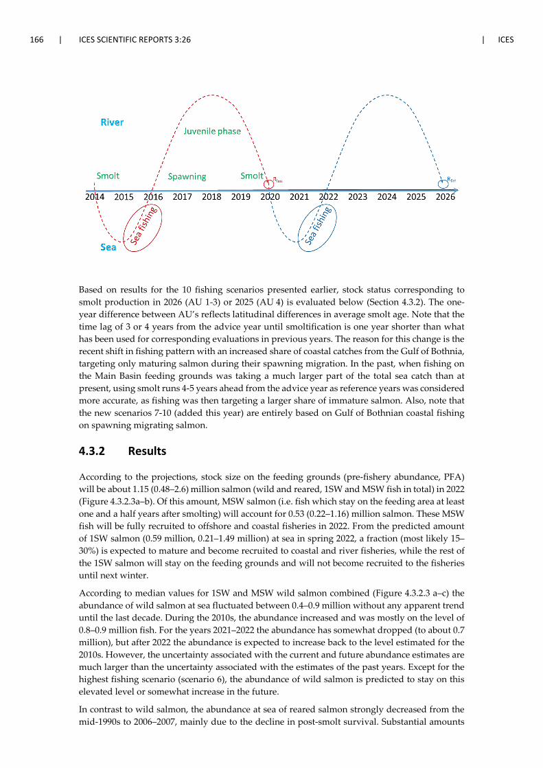
166 | ICES SCIENTIFIC REPORTS 3:26 | ICES
Based on results for the 10 fishing scenarios presented earlier, stock status corresponding to smolt production in 2026 (AU 1-3) or 2025 (AU 4) is evaluated below (Section 4.3.2). The one-year difference between AU’s reflects latitudinal differences in average smolt age. Note that the time lag of 3 or 4 years from the advice year until smoltification is one year shorter than what has been used for corresponding evaluations in previous years. The reason for this change is the recent shift in fishing pattern with an increased share of coastal catches from the Gulf of Bothnia, targeting only maturing salmon during their spawning migration. In the past, when fishing on the Main Basin feeding grounds was taking a much larger part of the total sea catch than at present, using smolt runs 4-5 years ahead from the advice year as reference years was considered more accurate, as fishing was then targeting a larger share of immature salmon. Also, note that the new scenarios 7-10 (added this year) are entirely based on Gulf of Bothnian coastal fishing on spawning migrating salmon.
4.3.2 Results
According to the projections, stock size on the feeding grounds (pre-fishery abundance, PFA) will be about 1.15 (0.48–2.6) million salmon (wild and reared, 1SW and MSW fish in total) in 2022 (Figure 4.3.2.3a–b). Of this amount, MSW salmon (i.e. fish which stay on the feeding area at least one and a half years after smolting) will account for 0.53 (0.22–1.16) million salmon. These MSW fish will be fully recruited to offshore and coastal fisheries in 2022. From the predicted amount of 1SW salmon (0.59 million, 0.21–1.49 million) at sea in spring 2022, a fraction (most likely 15–30%) is expected to mature and become recruited to coastal and river fisheries, while the rest of the 1SW salmon will stay on the feeding grounds and will not become recruited to the fisheries until next winter.
According to median values for 1SW and MSW wild salmon combined (Figure 4.3.2.3 a–c) the abundance of wild salmon at sea fluctuated between 0.4–0.9 million without any apparent trend until the last decade. During the 2010s, the abundance increased and was mostly on the level of 0.8–0.9 million fish. For the years 2021–2022 the abundance has somewhat dropped (to about 0.7 million), but after 2022 the abundance is expected to increase back to the level estimated for the 2010s. However, the uncertainty associated with the current and future abundance estimates are much larger than the uncertainty associated with the estimates of the past years. Except for the highest fishing scenario (scenario 6), the abundance of wild salmon is predicted to stay on this elevated level or somewhat increase in the future.
In contrast to wild salmon, the abundance at sea of reared salmon strongly decreased from the mid-1990s to 2006–2007, mainly due to the decline in post-smolt survival. Substantial amounts
ICES | WGBAST 2021 | 167
of reared salmon are assessed to have recruited to the fisheries for short periods both in the early and the late 2010s, but the current abundance is estimated low and it is also predicted to stay low during the coming years. The combined wild and reared abundance (PFA) also declined sub-stantially from mid-1990s until 2006–2007, but thereafter the total abundance has somewhat in-creased (Figure 4.3.2.3a–c).
Because one of the simplifying assumptions of the modelled life cycle is that all salmon die after spawning, a lower maturation rate will increase the survival of the cohort to the next year com-pared to years with the same abundance but with average maturation. Similarly, a high matura-tion rate will decrease the abundance of MSW salmon in following years. Because of this feature, it is important to note that the predicted abundance may easily become over- or underestimated because of the (predicted) development of maturation rates.
Table 4.3.2.1a shows the predicted catches by scenario for the year 2022. The table also shows the predicted fishing mortalities, as well as the predicted number of spawners and number of non-harvested (surplus) reared salmon in 2022 for each scenario.
How the catch in each scenario would become divided between various fisheries and their com-ponents (commercial, recreational, reported, unreported etc.) depends on the applied manage-ment. Table 4.3.2.1b and Figure 4.3.2.9 show how the catch components have developed and what they were in the latest year (2020) with the available information. For instance, from the total combined sea and freshwater catch in 2020, 42%, 16% and 42% were taken by commercial, recreational sea and recreational river fisheries, respectively. During the last five years these pro-portions have been fluctuating without any trend, but the share of both types of recreational catches have increased so that in 2016–2018 their combined share was close to 40%, while in 2019–2020 their share exceeded 50%. From the total sea catch in 2020, commercial catch ac-counted for 73% (ranging between 73–84% during the last five years). Reported commercial catch accounted for about 81% (ranging from 55–83% during the last five years) of the total commercial sea catch (i.e. total fishery related mortality). Unreporting, misreporting and discarding in 2020 are considered to have taken 6%, 0.2% and 8% shares of the total commercial sea catch, respec-tively. Among these catch components, only misreporting has been varying considerably during the last five years (between 0.2–28%).
The scenarios 7–10 consider a situation, in which sea fisheries take place only on coastal waters, which means that almost the whole sea catch would be caught in subdivisions 29–31. In this sea area, about 90% of the total sea catch has been taken by commercial fisheries during the last five years. About 84% of this has been reported commercial catch. Among the rest of the components of commercial catch, unreporting has been accounting for the largest share (8–9%) (Table 4.3.2.1b).
Figure 4.3.2.4 illustrates the longer term development of future sea catches given each scenario. Note that in the scenarios 3–6 the sea catches are taken both by offshore and coastal fisheries, while in the scenarios 7–10 only coastal fisheries exist. In scenarios 3–6 the current fishing pattern is applied by keeping the relative differences between the harvest rates of various fisheries con-stant. Because of the sequential nature of fisheries, this application results in changes to the rel-ative share of catches between fisheries: the higher the total removal, the higher the proportion of catch taken by offshore fisheries (which catch fish first). This phenomenon does not occur in the scenarios 7–10.
Figures 4.3.2.5a–d present the stock-specific annual probabilities to meet RMSY under the scenar-ios 1–6, while Figures 4.3.2.5e–h present the corresponding probabilities under the scenarios 7–10. Tables 4.3.2.2 to 4.3.2.5 show stock-specific probabilities to meet Rlim and RMSY in the smolt production in the years 2026/2025 and five generations (G=6 years for the AU 4 stocks and 7 years for the AU 1–3 stocks) ahead from 2020, whose smolt production is used to evaluate current stock
168 | ICES SCIENTIFIC REPORTS 3:26 | ICES
status. As explained earlier (section 4.3.1), the stocks status measured from the smolt production in 2026/2025 reflects the direct, immediate effects of the 2022 fishing on salmon reproduction. Finally, Table 4.3.2.6 shows, what proportions of the 17 assessed stocks reach Rlim in 2026/2025 and 5 generations ahead from 2020, given different levels of certainty.
As expected, the lower the harvesting, the higher is the status of stocks. For some of the stocks, river fishing alone (scenario 2) has a visible effect on the probability to reach the reference points compared to zero fishing scenario (scenario 1). This is the case especially among the stocks with the weakest status; therefore restrictions or ban of river fishing (like already enforced in Kågeäl-ven, Ljungan, Testeboån and Emån) are likely to improve the status of the weakest stocks. How-ever, for most of the stocks there is little difference in the predicted stock development among the scenarios with no fishing or removals below 100 000 salmon, i.e. in the scenarios 1–3 and 7-9. The effects of harvesting on future development and stock status become widely significant in scenario 6, in which total sea removal is assumed as high as 200 000 salmon. For a number of stocks, the future probabilities to reach Rlim and RMSY notably decrease under this scenario. The scenarios 4–5 with total sea removals of 100 000 and 150 000 respectively, which roughly corre-spond to the most recent harvest levels, indicate gradual improvements (higher probabilities to reach Rlim and RMSY compared to the year 2020) for most of the stocks, whereas some of the health-iest ones maintain their current high status.
All the stocks are expected to reach Rlim with >0.5 probability by 2026/2025 in the scenarios 1–3 and 7-9 (Table 4.3.2.2). Five salmon generations ahead from 2020 Rlim is predicted to be reached with >0.5 probability in all other stocks and scenarios, except in Ljungan under the scenario 6 (Table 4.3.2.3). Moreover, the probability to reach Rlim is predicted to mostly increase in all other scenarios except in the scenario 6. The long-term prediction indicates, which level of harvesting allows stocks to gradually continue their recovery, as summarized in the above paragraph.
As expected, RMSY has been and will be reached by lower probabilities than Rlim (Table 4.3.2.4). Decreases in the probability of some rivers to reach RMSY in 2026/2025 and 5 generations ahead compared with the current situation occur mainly in the scenario 6, but in some cases also in the scenario 5 and in a couple of cases even in all the scenarios (Table 4.3.2.4-5). In the other scenarios than 5 and 6, the drop in the probability is so small that it is explained by more accurate estimates of smolt runs in 2020 (from which year data exists) than in the future (which are predictions) (Figure 4.3.2.6).
Among the scenarios 7–10, which assume no offshore fishing and therefore in practice move sea harvesting to the spawning runs of AU 1–3 stocks, there are only small and sometimes almost unnoticeable differences in the AU 1–3 stocks’ status with the given range of removals (from 25 000 to 100 000 salmon). This results from the altered size/age selectivity of this fishing pattern, as well as it indicates a greater resilience among the northern (AU 1–3) stocks to harvesting, compared to the southern (AU 4, possibly also AU 5) stocks which are not harvested at sea in these scenarios. Within the Gulf of Bothnia, the weakest stocks of the Gulf are located in the AUs 2-3, which are not harvested by coastal fishing as much as the AU 1 stocks because fishing within the Gulf is aggregated to the coastal stretches where only AU 1 stocks are present (section 4.5.3.2). This further explains why the coastal fishing scenarios do not result in more negative effects among these stocks. Instead, the scenarios 7-10 predict somewhat stronger improvements to the status of the southern stocks than the scenarios with the current fishing pattern and similar levels of total removal (scen 3 vs. scen 8 and scen 4 vs. scen 10; Tables 4.3.2.2–4.3.2.5, Figure 4.2.3.5a–h).
When comparing the total smolt production in each AU in the year 2020, 2026/2025 and five generations ahead from 2020 vs. the combined total AU specific Rlim, all AUs have reached Rlim in 2020 with high probability (prob 0.86–1) and they are predicted to maintain high status also in the future (Tables 4.3.2.2 and 4.3.2.3). However, in the scenarios 5–6 the probability for AU 3
ICES | WGBAST 2021 | 169
to reach Rlim somewhat decreases. When comparing the smolt production in each AU with RMSY, the corresponding probabilities are clearly lower than those for Rlim both in the current and the future situations (Tables 4.3.2.4 and 4.3.2.5). The probabilities mostly increase (or stay on the current level) in scenarios 1–4 and 7–10, while in scenario 6 probabilities decrease in most of the AUs.
Currently (year 2020), 53% and 82% of the 17 assessed stocks have reached Rlim with probabilities above 90% and 50%, respectively (Table 4.3.2.6). Interestingly, the proportion of stocks which have reached Rlim with at least 50% probability is predicted to increase substantially even in the scenarios with the highest fishing mortality. The proportion is predicted to increase especially over the long term (after five generations this proportion is 94% in the scenario 6, for example). On the other hand, the proportion of stocks which will be above Rlim with high (>90%) probability is predicted to decrease in the scenario 6. Of the scenarios with the most similar removals to the 2021 advice (4 and 5), the scenario 4 allows two additional stocks and the scenario 5 allows one additional stock to reach Rlim with 90% probability in 2026/2025 (compared with current status). The proportion of stocks having very high (>95%) probability to be above Rlim increases in the scenarios 1-3 and 7-9, but this proportion begins to decrease in the rest of the scenarios. Among the scenarios 7-10 with only coastal fishing the proportions to reach Rlim increase in all except one case: in short-term the proportion of stocks exceeding Rlim with >95% decreases by one stock in the scenario 10. To summarize, these results show how most of the stocks which are currently recovering tend to recover also in the future, whilst increases in harvesting generally prevent stocks to hold high status with very high probability.
As expected, changes in fishing have the smallest effect on those stocks that are close to their PSPC (Tornionjoki, Kalixälven, Piteälven, Byskeälven, Mörrumsån). Because the overall level of harvesting is low or moderate in these scenarios compared to historical levels, the examined range of fishing mortalities (except the most extreme scenarios 1, 2 and 6) only results in modest impacts on the chances of reaching the reference points. Future predictions about smolt abun-dance are naturally more uncertain than the estimated abundance until 2020 (Figure 4.3.2.6). However, in those stocks which are close to their PSPC, also the predictions are rather certain, indicating that smolt abundance will stay close to PSPC in these rivers under different fishing scenarios.
Figure 4.3.2.7a-d shows longer term predictions in the river-specific smolt and spawner abun-dances for three scenarios (1=zero fishing; 4= 100 000 sea catch; and 6= 200 000 sea catch). The two most extreme scenarios (1 and 6) illustrate the predicted effects of contrasting amounts of fishing.
4.4 Additional information affecting perception of stock status
This section focuses on auxiliary information of importance for a complete evaluation of the cur-rent stock status. In particular, we highlight information about diseases and other factors that may affect development in stock status, but which are not fully taken into consideration in the current modelling. Likewise, weaknesses in input data and/or difficulties to take into account certain river-specific issues in the modelling might affect the precision of status evaluations, and in the worst case introduce biases. Such shortcomings in the current assessment model are also discussed in this section.
170 | ICES SCIENTIFIC REPORTS 3:26 | ICES
4.4.1 Potential effects of M74 and disease on stock development
Many of the M74-fluctuations seen since the early 1990s have tended to last for some years before changing in direction (Figure 3.4.1.3). After a period with very low M74 abundance in 2011–2015, mortalities increased to higher levels in 2016–2018. In 2019, M74 related mortalities decreased considerably, and mortalities among offspring hatched in 2020 were even lower. The latest thia-mine analyses of eggs spawned in 2020 indicate that M74 mortality among offspring is predicted to decline to close to zero in 2021. Despite the recent positive development, the future occurrence and development of M74 is difficult to predict, which introduces uncertainty in forecasts of the development of salmon stocks. The disease outbreaks reported in several rivers in recent years (Section 3.4.4) is also a concern for the future. The cause(s) of the disease is still unknown, and to accurately quantify the amount of affected or dead salmon in a river appears difficult, if at all possible.
To quantify the effects of health issues among spawners on the recruitment in rivers is difficult. Existing information indicates that M74 or disease among spawners mainly affect number of eggs deposited or hatched or the number of dispersing fry. That is, losses seem to take place before the offspring reach stages with highest density-dependent mortality. Therefore, a stock with high status is expected to show more resilience against various events that negatively affects early reproduction (i.e. from egg deposition to dispersal of fry), because these effects may partly be compensated by reduced density-dependent mortality among the offspring. In contrast, weaker populations are not expected to have similar ‘buffers’ against such losses.
Average salmon 0+ parr densities in many rivers decreased in 2016–2018 compared to the histor-ically high densities observed around year 2015. In 2019 and 2020, parr densities again increased in many rivers. Part of these fluctuations may be explained by generation effects, i.e. variation in year-class strength among spawners, but mortality due to M74 and/or other disease outbreaks is likely also part of the explanation. Compared to other rivers, the very low parr densities recently observed in Vindelälven and Ljungan are exceptional. In Vindelälven, the average 0+ density dropped drastically, from ca. 40 parr/100 m2 in 2015 to only one parr/100 m2 in 2016, and re-mained at very low levels until 2019 (Table 3.1.2.1). The decline likely reflects a combination of factors. In 2015, only 790 females were counted in the Norrfors fish ladder, which represented 18% among MSW salmon and 11% of the total spawning run (if assuming 6% females among grilse). In 2016, the number of females counted was higher (2741), but a large proportion of the salmon passing the ladder had severe skin problems (fungus infections) and many died soon after having been counted. Female numbers again decreased to 908 in 2017 and 728 in 2018, which represented only 32% and 26%, respectively, among MSW salmon. There are no observa-tions of such skewed sex ratios in the sea or at the river mouth of Umeälven, or in other rivers. Hence, the recent disease problems in Ume/Vindelälven seem to have prevented particularly females from reaching the spawning areas.
In 2019, the number of MSW Vindelälven salmon counted at Norrfors increased significantly. In total 3389 females, representing 33% of the MSW salmon, passed the counting site. Salmon still expressed symptoms of having health problems, but these were mainly observed during the early part of the migration period. The increase of female MSW salmon in 2019, resulted in a pronounced increase in densities of 0+ salmon in 2020. In 2020, the number of ascending MSW females increased further, indicating that the negative trend in recruitment observed in recent years has likely reversed into recovery phase. Furthermore, as described above, the M74 situa-tion has generally improved with low fry mortalities in 2020 (Table 3.4.1.1) and even lower pre-dicted mortalities in 2021, which will likely improve possibilities for recovery of this river stock.
Also, in Ljungan average 0+ salmon densities in 2017 and 2018 were exceptionally low (<1 parr/100 m2) compared to other rivers in Gulf of Bothnia. There was a slight increase in 2019 and
ICES | WGBAST 2021 | 171
2020, but the abundance of 0+ parr is still low compared to that of the preceding years (average density of 61 0+ salmon in 2014–2016; Table 3.1.3.1). Notably, the collapsed parr density in 2017 followed after a year with many dead salmon observed in the river, combined with a high ex-pected level of M74-mortality. The very low parr densities in Vindelälven (2016–2019) and Ljun-gan (2017–2020) are expected to result in a successive reduction in smolt production from 2019 and a few years onwards, affecting pre-fishery abundance of salmon from these two rivers from 2021. Because of the exceptional situation for these two rivers, local fishing restrictions, aimed at protecting ascending spawners in the estuarine sea during upstream migration, were enforced in 2019 and were in operation also in 2020. Most likely, these fishing restrictions will continue in 2021.
Although the FLHM cannot in its current form incorporate all details of the specific events af-fecting salmon stocks in Ume/Vindelälven and Ljungan, their consequences for recruitment are incorporated mainly via the time-series of smolt production (including predictions of the near-future production) based on parr densities fed into the river model, as explained and shown in the Section 4.2.2. Also, the recent low success of females to reach spawning grounds in the Ume/Vindelälven is incorporated, but currently there are no methods for predicting the future development of health problems.
4.4.2 Biases in stock status evaluations
The precision in status evaluations of individual river stocks depends to a large extent on the amount of available data. Data from several life stages (parr densities, smolt numbers and num-ber of ascending spawners) and long time-series increase the possibility for an accurate status evaluation, whereas status evaluations of river stocks for which only information on parr densi-ties and/or short time-series is available becomes more uncertain. Also, river-specific factors may introduce uncertainties and/or biases in status evaluations. Migration obstacles, for example fish ways at dams, affect migration possibilities and/or survival of spawners and smolts to a varying extent. If not accounted for (e.g. because of lack of information), such factors may introduce bi-ases in status evaluations. For most stocks included in the FLHM, status evaluations are thought to be reasonably accurate without any severe biases. A few exceptions exist, however, among which particularly Testeboån and Piteälven stand out. A common denominator of these two riv-ers is the occurrence of dams which (to a largely unknown extent) affect migration possibilities and survival of both upstream and downstream migrating salmon. Weaknesses in input data and difficulties to take into account such river-specific issues in the modelling of these two stocks are discussed in more detail below. Although the status evaluations for Testeboån and Piteälven seem to be particularly affected by problems related to migration obstacles, similar issues may at least to some extent exist also in other rivers.
Testeboån was included in the FLHM for the first time in the assessment carried out in 2019. As described in ICES (2019), the PSPC posterior was heavily updated downwards, which resulted in a surprisingly high status of this new wild salmon river, given that salmon parr densities are still comparably low in substantial parts of the river system. The updated PSPC was thought to result from the omission of spawner count data at that time. In 2020, the FLHM was not updated. This year, spawner count data for years 2016–2020 have been included in the model for the first time, but the PSPC posterior was again heavily updated downwards, resulting in high estimated stock status, similar to the 2019 assessment results. Expert opinions on PSPC in combination with empirical data on the amount of out-migrating smolts, indicate that smolt production in recent years has fluctuated between 20–40% of the PSPC, which clearly deviates from the assessment results suggesting that current smolt production has already approached the river’s production potential.
172 | ICES SCIENTIFIC REPORTS 3:26 | ICES
The reason for the biased results is still not fully understood. A possible explanation is that the time-series on spawner counts is still too short (2016–2020) to provide enough information on the stock–recruit relationship in the river (there are currently only two spawner-recruit data pairs, since only offspring from reproduction in 2016 and 2017 have so far (2020) left the river system as smolts). The possibility for ascending spawners to find their way up and past the power plant in Strömsbro (where the fish counter is situated) to reach the main reproduction areas probably varies considerably between years depending on variation in water flow and op-eration of the power plant. Thus, recruitment of smolts may to a large extent be dependent on migration possibilities rather than the absolute number of spawners that entered the river mouth a few years earlier. The FLHM may interpret this apparent lack of correlation between ascending spawners and subsequent smolt production as if stock status is high (a smolt production close to PSPC). If so, the posterior PSPC may then be updated downwards to match smolt abundances backed up by empirical data. It is also possible that a lack of flexibility in the FLHM when it comes to stock-specific differences in vital rates may affect estimation of stock–recruit parame-ters for river stocks with few stock–recruitment observations. Spawner counts in 2018 (n=22) and 2019 (n=177) represent rather extreme values from a historical perspective, and the resulting smolt production in 2021 and 2022 will hopefully provide useful information on the stock–recruit dynamics, which, in turn, may result in more realistic estimates of the production potential and stock status in the coming years. Until then, status evaluations and projection results for Testeboån must be viewed with caution.
In the 2019 assessment, the modelling of Piteälven was changed so that observations on spawner counts were used directly in the FLHM instead of using them to produce smolt production priors as earlier. The reason for this change was to avoid making assumptions about stock–recruitment parameters outside the model when converting from spawners to smolts. As a consequence of this change, estimates of spawner and smolt abundances as well as stock–recruit parameters were significantly updated (higher stock–recruit steepness, lower PSPC), resulting in changes in status evaluation as compared to the previous year’s assessment. Based on fragmented inde-pendent data currently not used in the model, there is a concern that the status for Piteälven is biased upwards. The reason behind this bias is not known, but similarly as for Testeboån, it may be partially explained by insufficient flexibility in modelling of vital rates and between-river var-iability in the FLHM, which means that smolt-spawner survival is driven by data from other, not necessarily similar rivers. It is also possible that migration problems at the dam at Sikfors (located below the reproduction areas) introduce a similar phenomenon as in Testeboån, i.e. that annual variation in recruitment of parr and smolts to a large extent depends on varying migration pos-sibilities for spawners in the river rather than the absolute number of ascending spawners at the river mouth. As discussed above, the resulting weak correlation between ascending spawners and subsequent recruitment may be interpreted by the model as if the production level is close to PSPC. Although the working group has planned to evaluate the way Piteälven is handled in the FLHM and explore alternative modelling options, this work has not yet been carried out due to time constrains. Therefore, status evaluations and projection results for Piteälven should be viewed with caution.
Independent information, such as river catches and results from genetic mixed-stock analyses from the Main Basin (ICES, 2014), indicate that the smolt production in Ljungan is likely under-estimated by the assessment model, which may also affect status evaluations to an unknown extent. The main reason for the bias is that Ljungan is difficult to electrofish and it is unclear to what extent electrofishing data represent the true abundance of salmon parr. As only electrofish-ing data is currently available from this river, the plan is to start counting smolts in the near future. Until then, smolt production estimates and status evaluations of this river stock should be viewed with caution.
ICES | WGBAST 2021 | 173
4.5 Future management of Baltic salmon fisheries
4.5.1 Current management system
The current management of Baltic salmon is based on two management areas, only one quota (TAC) in each of them, which regulate sea and coastal mixed-stock fisheries targeting both weak and strong wild stocks as well as reared salmon. All wild salmon stocks were heavily overfished and severely depleted less than three decades ago, after which they have recovered thanks to strengthened fishing regulations. However, many (weak) stocks are still in their recovery phase. So far, no ‘rules’ or guidelines exist for how fast (within which time frames) weak salmon stocks should recover, or when a certain proportion of all stocks should have obtained their manage-ment goal. Therefore, the ICES catch advice for the commercial mixed-stock fishery on Baltic salmon has for many years been associated with some degree of subjective consideration regard-ing trade-offs between time to fulfil management objectives and exploitation possibilities. The biological basis for the advice has been that the commercial sea fishery should be kept low enough to allow for a gradual recovery of all wild stocks, including the weakest ones. The ad-vised fishery has not been zero, however, thus allowing for some exploitation which likely has slowed down the recovery rate.
As presented in Section 4.2, the latest status evaluations show that six of the 17 analytically as-sessed stocks in AU 1–4 are at or above the stock-specific MSY level (RMSY) with relatively high (>70%) probability, while weaker stocks, which have not yet obtained their management objec-tives have had a positive development and are expected to show continued recovery under the current exploitation rate and fishing pattern. A few exceptions exist, represented by stocks that have been affected by health problems in recent years (Section 4.4.1). The temporal decline in production in these rivers is, however, not fishery related and would likely have been of similar magnitude also in a situation with a lower exploitation rate.
In contrast to AU 1–4, salmon stocks in AU 5 are not analytically assessed, and a majority have not responded positively to previous reductions in fisheries exploitation. Status evaluations of AU 5 stocks are uncertain and to a large extent dependent on expert opinions, and stock projec-tions needed to evaluate effects of different exploitation levels on stock development are thus not possible. In addition, problems in the freshwater environment such as reduced migration possibilities, poaching, poor spawning and rearing habitats, eutrophication, and bad water qual-ity, are likely affecting the stock status and development of many AU 5 stocks (e.g. ICES, 2014). This raises questions to what extent salmon stock dynamics in AU 5 are regulated by riverine conditions in relation to sea survival. This distinction is critical in order to steer management actions towards either improving riverine conditions (which, except poaching, falls more on en-vironmental management), or implementing further measures by international fisheries man-agement.
Recent calculations based on limited data from four AU 5 stocks (ICES, 2020b, see below) demon-strated some positive correlation between sea survival and recruitment (parr densities), indicat-ing that sea survival probably has played a role in explaining the dynamics of at least some AU 5 stocks. These calculations further showed that for the period up to and including 2018, around 1000–1500 wild AU 5 spawners were annually harvested by offshore fishing in the Main Basin, whereas 3000–4000 salmon returned to the rivers (ICES, 2020b). Thus, a complete phasing out of this sea fishery would likely result in a significant increase in spawner numbers. Note, however, that the latest estimates of harvest rate in offshore fishing (which catches also AU 5 stocks) in 2019 and 2020 are significantly lower than for previous years (Figure 4.2.3.9). Furthermore, pro-nounced annual variation in recruitment indicates that also river conditions play a significant
174 | ICES SCIENTIFIC REPORTS 3:26 | ICES
role. It is therefore likely that different areas/rivers need different measures to improve the situ-ation for weak AU 5 stocks, of which reduced exploitation at sea constitute one of several possi-ble management actions. Non-fishery related actions are likely also required to enable these stocks to recover.
So far, salmon stocks in AU 6 (Gulf of Finland) are also without an analytical assessment. In contrast to the situation in AU 5, the wild AU 6 stocks have shown a positive development since the late 2000s with a presumed high current stock status. Little is known about the harvest rates of AU 6 salmon at sea. However, various pieces of information indicate that these stocks have different migration routes than salmon in the other AUs, as they mainly seem to stay for feeding in the Gulf of Finland or further to the north in the Main Basin.
4.5.2 Evaluation of a new multiannual management plan
During the years 1997–2010, the management of salmon in the Baltic Sea was covered by the IBSFC Salmon Action Plan (SAP). The objective of this plan was to re-establish/recover wild Bal-tic salmon to attain, for each salmon river, a natural smolt production of at least 50% of the river-specific (best estimate of) PSPC until 2010. In 2008, the SAP had already become obsolete relative to fishing, and the European Commission decided to develop options for a new SAP to address all life stages of salmon and all human impacts. Based on the results of an ICES workshop (ICES 2008) and a subsequent consultation process, an EC proposal for a multiannual plan was pre-sented in 2011 (EC, 2011). This proposal was never realized, due mainly to political reasons.
A few years ago, managers from Baltic Sea countries (BALTFISH) finalized an updated draft of the original EC proposal from 2011. In 2018, ICES received a special request from the EC to eval-uate parts of the plan proposed by BALTFISH. The work to respond to the special request was carried out in an ICES workshop (WKBaltSalMP; ICES, 2020b) that included two meetings at-tended by scientific experts, national managers and stakeholder representatives. As requested, existing and alternative reference points for the assessment of stock status and fishing opportu-nities were examined. The existing targets formulated in terms of smolt production (50% and 75% of PSPC) were found to be inconsistent with the overall objective in the draft plan of achiev-ing MSY, as they in most cases deviate from the stock-specific targets corresponding to this level (RMSY). A precautionary reference point (Rlim) was further evaluated, defined as the lowest level of smolt production from which a stock is expected to recover to RMSY in one salmon generation, if all fishing was completely closed (ICES, 2020b). Based on these results, ICES advised to use stock-specific smolt production targets (RMSY and Rlim) as future reference points for Baltic salmon (ICES, 2020c).
A further request to ICES was to evaluate the recovery rate of individual wild salmon stocks under alternative fishing scenarios. Simulations developed specifically for the workshop allowed evaluation of such rates for river stocks with analytical assessment. Neither the EC request nor the draft multiannual plan specified criteria for when targets have been reached (i.e. the proba-bility of achieving the target). Therefore, ICES was not in a position to advise on when (or if) a stock had met one or several of the alternative targets. Instead, the probabilities of the smolt production being above alternative reference points for each stock were provided for a range of fishing scenarios. For river stocks without analytical assessment, correlative analyses between total estimated sea survival and recruitment over generations were performed in order to eval-uate to what extent sea fisheries may affect dynamics of these stocks.
A simplified stable state population dynamics model was constructed to study trade-offs be-tween mixed (sea) and stock-specific (river) fisheries in terms of achievable catches and propor-tions of stocks above/below reference points. This analysis illustrated that when the mixed-fish-ery harvest rate is kept low, all river stocks may achieve MSY, whereas when this harvest rate
ICES | WGBAST 2021 | 175
increases, less resilient stocks fall below this target. However, the fact that less productive river stocks fall below MSY (and may go towards extinction if the fishing mortality increases) does not make a noticeable difference to the total yield. Hence, there exists an inbuilt conflict between overall production and conservation aims that can only be resolved if mixed-stock fisheries for Baltic salmon are kept at a low level. The most efficient way to utilise the total resource is a stock-specific management, where stocks are harvested separately according to their respective char-acteristics and capacities.
Finally, the report from WKBaltSalMP also contained general comments on the draft manage-ment plan. The workshop identified that the draft had a strict focus on commercial sea fisheries, although the relative importance of recreational fisheries for Baltic salmon has increased signifi-cantly over time. The current two management units for EU commercial fisheries (Subdivision 22 to 31 and Subdivision 32) were also maintained in the draft, whereas evidence is accumulating that salmon are migrating between these areas more than previously recognized. The draft plan further did not address management of hatchery reared Baltic salmon more than marginally, despite large ongoing releases for various purposes in most countries.
In 2020, the European Commission decided to withdraw its originally proposed multiannual management plan for Baltic salmon from 2011 (EC, 2020). At present, it is unclear if, or when, a new proposal may be developed, and to what extent such a new draft will contain elements from the previous ones.
4.5.3 Fishing possibilities under alternative management strategies
Managing the Baltic salmon, with its many genetically distinct river stocks with varying status, is a challenge. The species is exploited both in the sea, along the coasts and in rivers, where the sea and coastal fisheries mainly target mixed stocks. Despite this complexity, the current man-agement system is based on only two TACs, one for SD 22-31 and one for SD 32. As indicated above, under current conditions with considerable variation in stock status, this rather blunt management system is associated with a difficult trade-offs between exploitation possibilities, the time required to achieve management objectives, and protection of weak stocks. Many of these difficulties may be overcome by the development of a more stock-specific management system, enabling fishing opportunities to be better-adapted to the situation for individual stocks. This could be achieved by spatial management of the sea and coastal fisheries, with the aim to steer exploitation towards harvesting of reared salmon and stronger wild stocks, thereby reduc-ing the exploitation of weak stocks.
The current assessment results with future projections (Section 4.2–4.3) and analyses carried out in WKBaltSalMP show that virtually all river stocks in AU 1–4 are expected to have a positive future development under the current (historically low) fishing pressure. At the same time, for weak stocks it may take considerable time (more than five salmon generations) until recovery to RMSY with high probability, also in a situation with no fishing at sea. For some rivers, there are additional river-specific factors (e.g. disease outbreaks) explaining the currently low status and slow recovery rate, which are likely of larger importance than fishing mortality for the future development of these stocks. For the weak AU 5 stocks, the lack of an analytical assessment pre-cludes reliable status evaluations and future stock projections under different fishing scenarios. However, as mentioned in Section 4.5.1, there are reasons to believe that a reduced offshore fish-ing pressure in the sea would improve recovery rate of these stocks, although management measures in the freshwater environment may be of equal or even larger importance for some rivers.
Under current conditions, one spatial management option could be to phase out commercial and recreational mixed-stock offshore fisheries in the Main Basin (that harvest all the weak stocks)
176 | ICES SCIENTIFIC REPORTS 3:26 | ICES
while keeping exploitation in the Gulf of Bothnia at the current level. As AU 4-5 stocks are not present in Gulf of Bothnia during the fishing season (see Section 4.5.3.1 for a review of genetic mixed stock analyses), such a change of the fishing pattern would reduce the exploitation of these weak stocks to a minimum without jeopardizing the management objectives of the gener-ally healthier AU 1–3 stocks (see scenarios 7–10 above). With respect to the recreational trolling fishery at sea in the Main Basin, which is a pure mixed-stock fishery that has expanded over time, one management option instead of a total ban could be to only allow landing of fin-clipped (reared) salmon. Such a measure has been implemented in Sweden since 2013. If followed by additional countries, the fishing mortality on several of the weakest wild salmon stocks would likely be reduced (although levels of post-release mortality for salmon caught in trolling are largely uncertain, and studies of this topic are warranted).
The coastal fishery may also be managed spatially to become more stock-specific than at present. In Gulf of Bothnia, this can be achieved by steering the coastal fishery towards estuaries of salmon rivers with healthy stocks and/or coastal areas where salmon from weak stocks is rare according to model results based on genetic data and other information (Whitlock et al., 2018; Dannewitz et al., 2020a,b; Section 4.5.3.2). Coastal fisheries in the Main Basin may also be man-aged spatially to avoid exploitation of weak stocks. However, there is a lack of knowledge about the mixture of salmon stocks in space and time in this area, and studies similar to those carried out in the Gulf of Bothnia (Whitlock et al., 2018; Section 4.5.3.2) are needed to evaluate how dif-ferent coastal fishing scenarios in the Main Basin may affect the development of weak stocks.
In addition to the above management considerations regarding recovery of weak wild salmon stocks, the presence of a significant portion of reared salmon in the Baltic Sea should also be accounted for. As shown in Table 4.3.2.1, the different exploitation scenarios evaluated result in different “surpluses” of reared salmon spawners returning to rivers without being utilised in the fishery. As an example, the expected surplus of reared salmon in 2022 under a no-fishing sce-nario in the sea is about 51 000 salmon, whereas the expected surplus under scenario 4, which roughly corresponds to the realised exploitation rate in 2020, is approximately 25% lower (Table 4.3.2.1). As outlined below, the main purpose of the substantial releases of reared salmon is to compensate for lost fishing opportunities due to hydropower exploitation. However, continuous large-scale releases are also associated with genetic and ecological risks for wild salmon stocks. One management option aimed at increasing the relative exploitation of reared salmon could be to exclude certain fisheries (e.g. in estuaries of reared rivers) from the quota system, given that solid scientific information exists showing that reared salmon completely dominate in those catches.
4.5.3.1 Genetic mixed-stock analyses of Baltic salmon – a review
Stock proportions in commercial salmon catches from the Baltic Sea have been analysed as a part of annual WGBAST reports since 2005. Stock proportions have been analysed yearly for Finnish catches from the Gulf of Bothnia. Swedish catches from the Gulf of Bothnia were also analysed yearly as a part of the WGBAST reports until 2017 (ICES, 2017a). Stock proportions in Swedish coastal salmon catches have further been analysed for national reports in 2014 and 2015 (Öster-gren et al., 2014; 2015). Finnish and Estonian commercial catches from the Gulf of Finland were most recently analysed in 2019 (ICES 2019). Stock proportions in the commercial catches from the Main Basin have been analysed for the 2015 and 2017 WGBAST reports (ICES, 2015; 2017a). In addition, the presence of salmon from individual stocks in either commercial or experimental catches from the Baltic Sea have been analysed and presented in several peer-reviewed publica-tions (Koljonen and McKinnell, 1996; Koljonen and Pella, 1997; Pella and Masuda, 2001; Koljonen et al., 2005; Koljonen, 2006; Palm et al., 2008; Vuori et al., 2012; Whitlock et al., 2018).
ICES | WGBAST 2021 | 177
The estimates of stock proportions in commercial catches of the Baltic Sea as reported in the annual WGBAST reports (ICES, 2005–2020) are based on stock assignment with DNA-microsat-ellite data. In short, each sampled fish from commercial catches is genotyped with 17 microsat-ellite loci and the smolt age of each sampled fish is determined. The genotypes and smolt age are then compared to a baseline dataset, which consists of genotypes and smolt age distributions of different salmon stocks from different spawning rivers around the Baltic Sea. Based on the com-parison of genotypes and smolt age with the baseline data, each salmon from commercial catches is then assigned the most probable stock of origin. Presently, the baseline dataset consists of 4453 individual salmon from 39 individual stocks from six different countries, each genotyped with 17 microsatellite loci. The stock assignment is based on Bayesian inference as implemented in the software BAYES (Pella and Masuda, 2001), which allows integrating smolt age information into the stock assignment, making especially the distinction between wild and hatchery origin stocks more reliable (Koljonen, 2006).
In general, the reliability of stock assignment with 17 microsatellite markers combined with smolt-age data is quite high. For example, the mean proportion of times an individual was as-signed to a particular stock in 1 000 iterations of MCMC in the 2017 Gulf of Finland catch samples was 0.95 (N = 411 individual salmon). In the Bothnian Bay catch samples from 2020, the mean proportion of assignment to a certain stock was slightly lower, 0.88 (N = 111 individual salmon, regular fishing season), due to the genetic similarity of wild stocks from the Kalixälven and Tor-nionjoki rivers (see Miettinen et al., 2021) as well as the mixed genetic background of the river IIjoki hatchery stock (Säisä et al., 2003). It must also be noted that stock proportion estimates prior to 2008 were based on eight microsatellite markers, which is likely to reduce their power of res-olution, especially of genetically similar stocks.
The most comprehensive data on stock proportions in commercial catches are from the Gulf of Bothnia, where the stock proportions in Finnish catches from three fishing areas along the coast have been estimated annually for the past 20 years. In summary, the data show that the great majority of salmon caught by the Finnish commercial fisheries originate from wild stocks of riv-ers Tornionjoki and Kalixälven, and hatchery stocks with their genetic origin in the river Torni-onjoki (means in the regular fishing season 2009-2020: 68% wild stocks and 29% hatchery stocks). In addition, a small proportion of the catches originate in Swedish hatchery stocks (mean 2009–2020: 2%). Salmon originating in Swedish wild stocks other than river Kalixälven are only caught occasionally; their total proportion of the Finnish salmon catch in the Gulf of Bothnia always has been <1%. No salmon from AUs 4–6 have been encountered in the commercial catches from the Gulf of Bothnia. The proportion of wild stock salmon from the rivers Tornionjoki and Kalixälven has increased following the change in temporal fishing regulations implemented in Finland since 2017, which has allowed an earlier start of fishing with limited number of fykenets (mean pro-portion of wild stock salmon in the advanced fishing season catches 2017–2020: 78%). There is, however, annual variation in the proportions of wild and hatchery origin stocks in the catches (proportions in regular season catches from 2009–2020: wild origin 58%–82%, hatchery origin 18%–38%).
Stock proportions in Swedish commercial catches from the Gulf of Bothnia were last reported in the 2017 WGBAST report (ICES, 2017a). As for the Finnish Gulf of Bothnia catches, a large pro-portion of the caught salmon originated in the wild northernmost Bothnian Bay rivers Torni-onjoki and Kalixälven (63% in 2013–2016 Finnish catches, 38% in 2013–2016 Swedish catches). Compared to the Finnish catches, there were less salmon from the Finnish hatchery stocks (rivers Kemijoki, Simojoki, Iijoki, and Oulujoki). The other main difference was that in these Swedish catches, there were salmon from additional wild Swedish rivers, especially Byskeälven and Vindelälven (mean proportions in 2013–2016: 12% and 10%, respectively). In total, the proportion of wild salmon has been higher in the analysed Swedish catches from the Gulf of Bothnia (mean 2009–2016: 82%) than in the Finnish catches (mean 2009–2016: 70%) (ICES, 2017a). It must be
178 | ICES SCIENTIFIC REPORTS 3:26 | ICES
noted, however, that the Swedish catch data analysed until 2017 was just collected from a limited number of fishing sites, and that the stock composition estimates from the western Gulf of Both-nia are much more influenced by the geographic position than on the eastern side along the Finnish coast, where a more homogenous stock mixture is harvested (ICES, 2017a; below). Salmon from the weakest Swedish stocks have only appeared once in Swedish commercial catches in 2006–2016 in the Gulf of Bothnia (Ljungan: 1% in 2010). The only stock from AUs 4–6 that has been caught by the Swedish fishery in 2006–2016 in the Gulf of Bothnia has been the Finnish hatchery stock genetically originating in the river Neva (2% in 2007).
Stock proportions in the Swedish coastal fishery in 2013–2014 have been reported in a national report by Östergren et al. (2015). Compared to the above ICES-analyses, a significantly larger number of fishing sites distributed along the Swedish coastline were included (18 sites, whereof eight were sampled in both 2013 and 2014, comprising a total of 2 850 individuals; Östergren et al., 2015). The same genetic data from 2014 have also been analysed by Whitlock et al. (2018; in press) in peer-reviewed methodological studies on the integration of genetic analysis of mixed stocks with a population dynamics model. In these analyses, samples from the Finnish coastal fishery in the same fishing year were also included. The genetic data from 2013 and 2014 (in combination with catch data from 2019) have also been analysed, using the same model, in a national report focusing on stock composition in Swedish coastal catches (Dannewitz et al., 2020b, see Section 4.5.3.2).
The main difference between the stock abundance estimates in catches presented by Östergren et al. (2015), Whitlock et al. (2018) and Dannewitz et al. (2020b) compared to those for Finnish and Swedish sea catches reported in earlier WGBAST reports was that the coastal Swedish catches were mainly composed of salmon from the rivers (wild or reared) closest to the catch sites. Also, the river Kalixälven and Tornionjoki wild stocks, which dominate the Finnish and Swedish catches reported by WGBAST, were nearly absent in the Swedish coastal catches (other than in the catches from near their own river mouths). Whitlock et al. (2018) further showed that the migration patterns can vary greatly among different Baltic Sea salmon stocks, meaning that there may exist strong variation in stock compositions at different times in a given area. Combining genetic marker data with information on population dynamics and movement provides a means for temporal and spatial regulation of fishing efforts to target reared and healthy wild stocks while avoiding weak ones (Whitlock et al., 2018). See Section 4.7.1 for a discussion on future potentials of including results from the Whitlock et al. (2018) coastal model as prior information into the regular WGBAST stock assessment.
Estimates of stock proportions in Finnish commercial catches from the Åland Sea are available from 2000–2016 (ICES, 2017a). Again, the largest proportions in the catches are from the rivers Kalixälven and Tornionjoki wild stocks (means 2000–2016: 23% and 34%, respectively). There are also small, but yearly varying proportions of salmon from the northern Bothnian Bay stocks as well as from the stocks from Swedish rivers (all means 2000–2016: 0–6%).
Stock proportion estimates from catches in the Gulf of Finland have been last reported in the 2019 WGBAST report (ICES, 2019) and include Estonian (2016–2018) and Finnish (2009–2018) coastal fisheries. The stock with the largest proportion in the Estonian catches has been the river Kunda stock, which includes both wild and hatchery origin fish (mean 2016–2018: 40%). The catches have also included salmon from rivers Keila (wild origin, mean 2016–2018: 17%) and Narva (hatchery origin, mean 2016–2018: 12%). The Estonian catches have further included salmon from the wild and hatchery stocks from AU5: Salaca (wild origin, mean 2016–2018: 3%) and Daugava (hatchery origin, mean 2016–2018: 6%). The Finnish coastal catches from the Gulf of Finland are mainly comprised of stocked salmon of river Neva origin (mean 2009–2018: 49%) and salmon from the northern Bothnian Bay rivers (Tornionjoki, Kalixälven, Oulujoki, mean 2009–2018: 43%). Salmon from other Swedish rivers have only been found occasionally in these
ICES | WGBAST 2021 | 179
Finnish catches (<1%), and salmon from AU5 and AU6 rivers only have been found in the 2018 Finnish catch: Daugava, AU5, hatchery origin: 3% (95% Confidence bounds: 1–5%); Keila, AU6, wild origin: 1% (95% Cb: 0–2%).
Stock proportion estimates for the Main Basin salmon fishery include data from commercial catches in selected years from Danish (2006, 2010–2016), Finnish (2006–2007, 2009–2012), Latvian (2006), Polish (2006–2016), and Swedish (2006–2007, 2010–2012) offshore catches. Catch data from different countries have been pooled and analysed together for each year. The stocks with largest proportions in the Main Basin salmon catches have been the wild stocks from rivers Kalixälven and Tornionjoki (means 2006–2016: 14% and 37%, respectively) (ICES, 2017a). The rest of the catches have been mainly composed of salmon from Swedish wild and reared river stocks (mean proportions for each stock in 2006–2016: 1–6%). The catches from the Main Basin have also in-cluded a few salmon from the AU5 hatchery stocks of rivers Gauja, Daugava, and Neumunas (2006–2016 means: 0–1%; 95% confidence bounds always including zero). Salmon from the wild Salaca (AU5) and mixed Luga (AU6) stocks have also been found in low proportions (1–2%) in the Main Basin catches from 2006–2007 and 2010–2011 (ICES, 2017a).
Stock proportion estimates for different areas of the Baltic Sea have also been published in peer-reviewed publications by Koljonen (2006), Palm et al., (2008), Vuori et al. (2012), and Whitlock et al. (2018). Koljonen (2006) analysed stock proportions in catches from the Gulf of Bothnia, Gulf of Finland, Åland Sea, and the Main Basin with 8 microsatellite markers, and with a baseline of 32 stocks. The data are in large part the same that have been published in the WGBAST reports in 2005 and 2006 (ICES, 2005–2006). The catch data in the WGBAST reports are based on sam-pling of commercial catches in open sea fisheries in winter and early spring in the Main Basin and coastal fisheries in summer in other areas. Palm et al. (2008) used a slightly extended baseline data from Koljonen et al. (2008) to estimate stock proportions in catches taken in late autumn in 2002–2003 from the Main Basin. Their stock proportion estimates were very similar to those in Koljonen et al. (2006): most of the salmon were from the Bothnian Bay stocks. There were no salmon from the currently weak stocks of river Ljungan or Emån. The only AU 4–6 stocks that were present in the catches were the hatchery stocks of rivers Neva (stocked into Finnish rivers; 1%; PI: 0–3%) and Gauja (1%: PI: 0–3%).
Vuori et al. (2012) have in addition analysed stock proportions of salmon catches in late autumn and winter from the Bothnian Sea, Gulf of Finland, and the Main Basin. The catch data analysed by Vuori et al. (2012) are a combination of commercial catches and samples collected for scientific purposes in 2006–2007. The data in Vuori et al. (2012) provide information on migration patterns of salmon from Baltic Sea stocks, but does not reflect the proportions of different stocks in today’s commercial catches as there is no longer commercial fishing of salmon in autumn and winter in the middle and northern Main Basin and northern Baltic Sea. The largest numbers of salmon in the samples from the Main Basin were from the river Tornionjoki wild and hatchery stocks (63/141 salmon, 45%). The number of samples from the Bothnian Sea was low (n = 31) and in-cluded individual fish (1–6) from wild and hatchery stocks of Finnish and Swedish rivers, and a few fish from the mixed stock of the Russian river Luga (n = 2) and hatchery stocks of the Latvian rivers Gauja and Daugava (n = 1 and n = 3, respectively). The most numerous stocks in the sam-ples from the Gulf of Finland were the Finnish river Neva hatchery stock (30/55 salmon) and the mixed stock from the river Luga (15/55 salmon). The rest of the salmon in the Gulf of Finland catch samples were from hatchery stocks of rivers Narva (n = 2), Gauja (n = 1), and Daugava (n = 7).
Whitlock et al. (2018) estimated stock proportions in catches from 18 coastal fishing sites in Fin-land and Sweden. Their findings also followed those reported in the annual WGBAST reports: stock composition along the Finnish coastline was dominated by the wild Tornionjoki stock,
180 | ICES SCIENTIFIC REPORTS 3:26 | ICES
while the catches on the Swedish side were more mixed, local stocks well presented in the catches.
In summary, mixed stock genetic analyses of Baltic Sea salmon catches performed over several years show that salmon from the AU 4–6 stocks do not occur in catches of Åland Islands and Gulf of Bothnian coastal salmon fisheries that take place only in summer. The WGBAST full life-history model (that currently includes only AU1–AU4 stocks) is constructed accordingly (see Stock Annex). In the Gulf of Finland commercial fishery, AU5 and AU6 fishes occur in small proportions in Estonian catches. In the main basin, AU5 and AU6 fish are also caught only occa-sionally in very small proportions by the commercial fisheries. The weak stocks of the Swedish rivers Ljungan and Emån have only been present in the catches near their respective river mouths. Fisheries in these weak rivers are presently closed.
4.5.3.2 A model predicting stock composition and catches of individual stocks in the coastal fishery in Gulf of Bothnia
A modelling tool for utilizing genetic data to learn about spatial patterns in stock-specific abun-dances (Whitlock et al., 2018) can be used to support interpretation of genetic mixed-stock anal-yses for stocks in assessment units 1–4. This model takes into account a prior probability weighting based on stock-specific migration patterns to probabilistically assign individuals to stocks, which is expected to be more robust than assignment with an uninformative prior (Whit-lock et al., 2018). This “multistock migration model” has now been extended to a multiple year version that includes an observation model for catches in the Swedish and Finnish commercial coastal trapnet fisheries, allowing estimation of stock-specific catches and harvest rates in time and space (Whitlock et al., in press). It is important to note that the results from this model are not currently used in the assessment, but their incorporation is planned as a key model develop-ment task for the future (see Section 4.7).
The model currently estimates stock-specific abundances in time and space for 17 wild and ten hatchery-reared Baltic salmon (S. salar) stocks, including all wild stocks in assessment units 1–4. It spans the coastal fishing period, following the population dynamics of migrating reproduc-tively mature salmon between April 15th and August 18th in each year in 48 spatial areas, as they migrate north from feeding areas in the Southern Baltic (Main Basin), along the Swedish and Finnish coasts to their natal rivers for spawning. An observation model for microsatellite allele frequency data at 17 loci, sampled at multiple locations over the fishing season is used together with a genetic baseline to learn about stock composition in time and space.
The latest version of the multistock migration model can be used for exploring stock-specific migration paths, abundances and stock compositions of catches from different areas and times. As an example, Figures 4.5.3.2.1a–d show estimated spatio-temporal distributions of the abun-dance of maturing salmon from four river stocks (one per AU) during six consecutive fortnights. From such heat maps, it is evident that the spawning migration paths of different river stocks differ in time and space and become increasingly unique when salmon are approaching their natal rivers. Hence, stock compositions of catches are highly dependent on when and where those catches have been taken.
As another example, Figure 4.5.3.2.2 shows total and stock specific catches in 2019. The upper left panel shows total reported catches and illustrates the pronounced differences between coastal sections, with the largest catches taken close to the most productive wild and reared riv-ers in the north. The other three panels in Figure 4.5.3.2.2 show estimated numbers of salmon in the same total (2019) catches for the three weakest river stocks in each of AUs 1–3 respectively (Simojoki, Lögdeälven, Ljungan). In total, the proportion of salmon from those weaker river stocks is just approximately 1% or lower, and in some areas a particular stock may not be caught
ICES | WGBAST 2021 | 181
at all. For example, salmon from Lögdeälven and Ljungan are estimated to be absent in the large catches taken from the northernmost Gulf of Bothnia (Figure 4.5.3.2.2).
4.5.4 Challenges for Baltic salmon management
Both the management and scientific advice process related to Baltic salmon would benefit from a decided framework including rules and guidelines on management objectives for this species. Such elements may be regulated within a multiannual management plan, or as a part of the pro-cess when EC request advice from ICES. Regardless, a sustainable management of Baltic salmon and its mixed-stock sea and coastal fisheries, that accounts for both conservation needs and ex-ploitation possibilities, requires that the following aspects or trade-offs are carefully considered:
• Time for recovery. Fishing mortality is a factor that determines the recovery rate of weak river stocks. If the main goal is to reach management objectives as fast as possible, fishing mortality must be as low as possible. However, if the goal is to combine recovery with some continued exploitation, time for recovery will be longer (as shown in Section 4.3). This trade-off between conservation and exploitation needs to be decided by managers in terms of acceptable time frames with respect to recovery, which, in turn, is a prereq-uisite for the formulation of appropriate advice on fishing opportunities (given the de-cided time frames). A related, more technical aspect, which also needs to be considered, is with which probability management objectives should be fulfilled, as this will deter-mine the risk to fall below the management target (note that the Baltic salmon assessment to a large extent accounts for uncertainties in data and model parameters, which needs to be considered when deciding upon appropriate probability limits).
• Proportion of stocks above management target. Independent of exploitation rate and time frames for recovery, some wild river stocks will likely remain below management targets for various fishery-independent reasons, such as local environmental problems, health issues or because they represent “new” wild rivers stocks added into the assess-ment (e.g. previously potential rivers) with initially low status. In addition, colonization of new river areas (due to e.g. dam removals) will affect the production potential of a river. This affects stock status, because status is evaluated based on comparisons between current smolt production and RMSY, of which the latter is expected to be updated upwards when the estimated smolt production potential increases in the future. Therefore, man-agers need to decide on what may be perceived as an acceptable share of river stocks which, at any given time, are not likely to reach their management objective for reasons as those mentioned above.
• MSY vs. conservation targets. The concept of maximum sustainable yield (MSY) aims at producing a long-term sustainable catch as large as possible, and it does not explicitly account for conservation aspects. Thus, when a river stock is assessed to be below RMSY or Rlim, this does not necessarily mean that it is ‘threatened’ by extinction; in the case of RMSY it simply means that it cannot produce a sustainable catch of the same magnitude as the potential maximum. To evaluate the level of threat and what constitutes a mini-mum viable population size (MVP), additional biological factors need to be accounted for in a formal population viability analysis (PVA). Although no such analyses have so far been carried out for Baltic salmon, it seems likely that the number of spawners corre-sponding to MSY (and Rlim) in large salmon rivers is located above any minimum con-servation target. For certain small rivers it is possible, though, that a higher target than stipulated by MSY may be needed to reduce risks for local extinction or loss of genetic variation.
• Releases of reared salmon. The total amount of reared salmon released annually in the Baltic Sea (between 4 and 7 million smolts) has for several decades outnumbered the
182 | ICES SCIENTIFIC REPORTS 3:26 | ICES
amount of wild salmon smolts produced in rivers. Continuous releases of this magnitude are associated with biological risks, through genetic and ecologic interactions between reared and wild salmon and spread of disease (e.g. Araki and Schmid, 2010; ICES, 2016; Hagen et al., 2019; Östergren et al., 2021). The bulk of releases in the Baltic Sea area are carried out in rivers exploited by hydropower, with the aim to compensate fisheries for the loss of natural production and fishing opportunities. To decrease risks associated with such releases, it is important that release volumes are adapted to the exploitation level in the fishery, to reduce the amount of unutilised reared salmon that may interact with wild conspecifics. As reared salmon is an important resource for Baltic Sea fisheries that at the same time constitutes a biological risk for wild salmon, Member States in the Baltic Sea area should agree on how stocking activities with different purposes should be managed in the future, based on scientific information (ICES, 2020b). Such a long-term plan should also provide recommendations/guidelines for management of hatchery pop-ulations and stocking activities so that negative impacts on wild stocks are minimized.
• Bycatches of salmon. Salmon is by-caught in several Baltic Sea fisheries targeting other species, but such catch data are sparse and estimates of their true magnitude highly un-certain. In coastal fisheries with passive gears (nets, trapnets, etc.) the amount of by-caught salmon varies depending on place and time of the year. As an example, in the Swedish coastal fishery for whitefish (with trapnets), which takes place mainly during summer months, salmon are by-caught to an uncertain but probably large extent (Dannewitz et al., 2020b). These salmon must be released back if caught outside the salmon fishing season. Recent studies indicate that catch and release from the most com-monly used gear (Pontoon traps) results in reduced survival probabilities (Östergren et al., 2020). Therefore, a better understanding of the amount of by-caught salmon in differ-ent fisheries targeting other species is important to evaluate effects on the development of salmon stocks. Salmon is also bycaught in the pelagic trawling fishery for herring and sprat, but again reported bycatches likely represent gross underestimates of true levels. One main reason may be that the smaller salmon (post-smolts) remain unnoticed. A crude extrapolation, based on data from scientific pelagic trawl surveys, suggested that the annual bycatch of salmon in the commercial pelagic fishery may have ranged from around 50 000 individuals in the 1980s to almost 200 000 in the 2000s (ICES, 2011). A ma-jority of these estimated by-caught salmon comprised post-smolts, although a consider-able portion of larger adults also existed in the scientific trawl catches. Updated and more refined estimates of the amount of salmon taken as bycatch in the commercial trawling catches appear warranted, especially given plans to commence large-scaled pelagic trawling for three-spined stickleback to reduce biomass of that species (such pilot studies are currently planned) that may increase the amount of bycatch even further.
4.6 Conclusions
The pre-fishery abundance is expected to show a minor decline in 2021 and 2022, followed by a gradual increase in line with the projected smolt production. Therefore, with stable fishing mor-tality, a somewhat smaller catch would be caught in 2021-2022 than before or after these years.
Out of the 17 analytically assessed stocks, three (Lögdeälven in AU 2, Ljungan in AU 3, and Emån in AU 4) were below their Rlim in the year 2020 (Table 4.2.3.4a). Results from the stock projections indicate, however, that exploitation similar to the current realized total catch (most similar to scenario 4) will result in either a maintained or positive trend in status for almost all AU 1–4 stocks (Section 4.3.2). Positive or maintained trends in the status of the AU 1-3 stocks have been seen already in the past years (e.g. Figure 4.3.2.5a–e), apparently due to the gradually decreased overall exploitation (Figure 4.2.3.10). The development of a few river stocks, in particular
ICES | WGBAST 2021 | 183
Vindelälven and Ljungan, is expected to show a somewhat delayed and slower increase due to disease problems in recent years. For Vindelälven, however, two years of increased numbers of returning MSW females indicate that the health situation in this river may be improving.
All the AU 1–4 stocks are predicted to reach >50% of their Rlim in the scenarios 1–3 and 7–10 (Table 4.3.2.2). In other words, a total catch of at least 50 000 (scen 3) but less than 100 000 (scen 4) could be harvested in 2022 with the current fishing pattern to allow all the AU 1–4 stocks to reach their Rlim in the 2025/2026 smolt production. However, the current analytical assessment does not include the AU 5 stocks, for which sea migrations are restricted to the Main Basin (and partly the Gulf of Finland; see Section 4.5.3.1). Most of the wild stocks in this AU are considered to currently be below Rlim, according to expert based elicitations. Analyses performed in 2020 (ICES, 2020b,c) indicated that maintaining a mixed-stock fishery in the Main Basin would likely negatively affect the recovery of these weak wild stocks.
According to new scenarios added this year (7–10), evaluating consequences of a sea fishery con-fined to Åland Sea and Gulf of Bothnia where only AU 1–3 salmon are harvested during their spawning migration, up to 75 000 salmon could be harvested. Under this exploitation rate and a fishing pattern with no Main Basin offshore fisheries, Rlim is expected to be reached in the 2025/2026 for all the analytically assessed stocks (AU 1–4). Such a change in the sea fishery would also increase the protection of the weakest AU 5 stocks.
As observed in earlier assessments, projections under different exploitation rates (+/-50 000 salmon compared to the approximate current level of removal) indicate that such changes in the sea fishery are not expected to result in large changes on the status development of the AU 1–4 stocks, with differences mainly manifesting for weak stocks. This further indicates that fishing mortality is currently at a relatively low level in comparison to other (natural) sources of mortal-ity affecting the stock development. Obviously, probabilities to reach the smolt production tar-gets are higher for scenarios with lower exploitation, but differences between scenarios are rela-tively small except for the ones with a drastically reduced or increased fishing (i.e. scenarios 1, 2 and 6).
Although the AU 5 stocks are not analytically assessed, data on recruitment combined with ex-pert evaluations on production potential indicate no obvious recovery; most of these stocks are currently (year 2020) believed to be far below their MSY-level and most of them are also likely below their Rlim. AU 5 stocks have not generally responded positively to previous reductions in fisheries exploitation, although indications exist about positive effects of temporally increasing overall sea survival (survival from both the natural and fishing induced mortalities) on the re-cruitment among these stocks (ICES, 2020b). AU 5 stocks are exploited in the Main Basin by offshore commercial and recreational fisheries and in rivers by angling, indicating that current exploitation and natural mortality rates (at sea and/or in freshwater) has not allowed for their recovery. One management option to assist the recovery of the AU 5 stocks is to reduce or phase out the Main Basin offshore fisheries (as indirectly seen for AU 4 stocks, with similar migration pattern at sea, in the scenarios 7–10). As discussed above, however, several environmental factors acting during the freshwater phase are believed to affect the development of the AU 5 salmon stocks negatively in addition to sea fishing. Therefore it should be noted, that even without any fishery it may still take considerable time (several salmon generations) until the currently weak-est river stocks will recover.
In contrast to AU 5 stocks, wild AU 6 stocks have shown a positive development in recent years. The stocks of Kunda and Keila are with high certainty above their MSY level (considering that their current smolt production is at or near 100% of their expert elicited PSPC), whereas the stock status of Vasalemma is rapidly increasing. This indicates that the current exploitation level al-lows a successful recovery of the AU 6 stocks.
184 | ICES SCIENTIFIC REPORTS 3:26 | ICES
Following a temporary and modest increase in M74 in recent years, this mortality factor has again decreased to a very low level. Another factor influencing stock development is the health problem affecting adults that have been observed in certain rivers since 2014 (Sections 3.4.4 and 4.4.1). If these health-related problems should prevail or increase further this may result in de-creased status, particularly for weaker stocks, as well as reduced fishing possibilities, and may easily counteract any positive effects of e.g. good post-smolt survival.
For some weak stocks, additional measures (on top of restrictions through the TAC system) may need to be implemented on the national level to increase the number of spawners, for example by reducing fisheries in rivers or coastal areas where these stocks are currently harvested. For instance, fishing restrictions have been enforced in Vindelälven and Ljungan due to health prob-lems among ascending adults in recent years. Similarly, in Emån and in the recently appointed wild salmon rivers Testeboån and Kågeälven, a fishing ban on salmon has prevailed for many years to increase the recovery rate of these river stocks. A comparison of scenarios 1 (no fishing at all) and 2 (only river fishing allowed) illustrates the positive effects of river fishing regulations. Measures focused on the freshwater environment, such as work to improve river habitats and migration possibilities, may also be necessary. Thus, special actions directed to the weakest stocks which are not only fishery-related ones are likely required at any advised TAC level, es-pecially in AU 5 but also for a few weak rivers in other AUs, to enable these stocks to recover. Such work is already ongoing in several countries (see Chapters 2 and 3).
Several of the northern stocks are assessed to be close to or above the MSY-level, and the surplus produced by these stronger stocks could in theory be directed towards stock-specific fisheries. However, the current management system, with a single TAC for SD 22–31 that is set at a rela-tively low level (from a historical perspective) to safeguard weaker salmon stocks, prevents much of this surplus to be utilised by the commercial sea fishery. Similarly, a large proportion of reared salmon cannot be utilised today because reared salmon is included in the same TAC as wild salmon. Some of the advantages of changing the current management system can be seen in scenarios 7–10, in which the exploitation is focused on reared salmon and the strongest and largest wild stocks in AU 1–3, while the harvesting of the weakest stocks which are located in AU 4–5 is kept close to zero (at much lower levels as compared to under the current fishing pattern; scenarios 3–6).
Consequently, Baltic salmon fisheries management could be developed to become more stock-specific, by implementing more flexible systems for the regulation of fisheries with the aim of steering exploitation towards harvesting of reared salmon and stronger wild stocks and avoiding weak ones. This could be achieved through spatial management, e.g. by implementing area-spe-cific quotas and/or exclusion of certain single-stock fisheries from the quota system (such as fish-eries in estuaries of rivers with reared stocks). Integration of genetic data into population dy-namics models can provide information about stock-specific abundance patterns and harvest rates in time and space, allowing evaluation of spatio-temporal management measures. This creates the potential to move towards stock-specific management whilst maintaining some level of catches in mixed-stock fisheries, since fishing mortality can be directed towards certain stocks (and away from others) using knowledge of stock-specific migration patterns. Such tools are now available and have been applied to the coastal fisheries in Finland and Sweden (Section 4.5.3.2); these tools could be adapted to form part of the WGBAST assessment framework in the future. In contrast, the increasing recreational trolling in Main Basin is a true mixed-stock fishery where fully stock-specific harvesting is not possible. Regulations that only allow the landing of fin-clipped (reared) salmon, such as has been implemented in Sweden since 2013, may reduce fish-ing mortality of wild stocks by trolling if the post-release mortality is relatively low.
As outlined in Section 4.5, the current management of Baltic salmon lacks specific ‘rules’ or guidelines for how fast (within which time frames) weak salmon stocks should recover, and what
ICES | WGBAST 2021 | 185
proportion of all stocks should have obtained their management goal within a certain time. Therefore, under current conditions with only TAC regulated commercial sea fisheries and river stocks with varying status, any catch advice for the mixed-stock fishery on Baltic salmon will be associated with some degree of subjective consideration of trade-offs. Sustainable management of Baltic salmon and its mixed-stock fisheries, which accounts for both conservation needs and exploitation possibilities, requires that management accounts for the above and other aspects or trade-offs discussed in Section 4.5. A clarified framework on how to manage Baltic salmon, e.g. formulated within a multiannual management plan, would also be beneficial for the biological advice process related to this species.
4.7 Ongoing and future development of the stock assess-ment
4.7.1 Road map for development of the assessment
The tasks listed below refer to ongoing, planned and potential updates of the assessment meth-odology. The “Ongoing and short-term tasks” below are intended to be undertaken as part of routine assessment model development, while some of the longer term tasks may require even-tual benchmarking. A list of tasks for the next benchmark can be found in Annex 3. That list relates to evaluation of the methodology for assessing stock status including the new reference points, as well as development of an analytical model for AU 6 stocks.
Ongoing and short term
• Incorporating estimates of stock-specific exploitation rates in the coastal fishery. There is a need to replace the present (crude) assumptions about how coastal fisheries affect develop-ment of the river stocks with more precise stock-specific estimates as input in the assess-ment model. Stock-specific harvest rate estimates from a spatially and temporally-struc-tured Bayesian mixed-stock analysis (MSA)/population dynamics model for the coastal migration of spawning Baltic salmon (Whitlock et al., 2018) are now available (Whitlock et al., in press). Some development of the MSA model is first needed to ensure that data in the FLHM are not used twice (the current version of the MSA model uses posterior distributions for natural mortality and pre-season abundances from the FLHM).
• Improvement of the fishing scenarios. The current method to set up the fishing scenarios enables maintaining the same relative differences between harvest rates of different fish-eries. However, it would be more practical to be able to maintain this pattern in terms of the relative differences between the catches. Also, the amount of uncertainty related to each harvest rate/catch at different fisheries and scenarios should be made more con-sistent, as in the current method, uncertainty increases heavily when higher removal is assumed. The magnitude of the uncertainty has a direct effect on the probability of meet-ing the reference points at each scenario.
• Investigating the reasons for implausible status evaluations in rivers Testeboån and Piteälven. More analysis is needed to understand the implausibly high-status evaluations for rivers Testeboån and Piteälven. This will be initiated by comparing model structures with in-creased stock-specific variability in vital rates, to see whether such increased flexibility can offer any improvements.
• Adding annual variation to the catchability parameters of coastal trapnet and gillnet fisheries. Annual variation in these parameters would be allowed by utilising autoregressive pro-cesses with a lag of one year similarly as has now been done for offshore fisheries. How-ever, an assumption of equal catchabilities for wild and reared salmon cannot be applied
186 | ICES SCIENTIFIC REPORTS 3:26 | ICES
to the coastal fisheries, which may require testing several types of parameterisation to find a suitable version.
• Improved description of river fisheries in the FLHM and scenarios. River harvest rates are cur-rently assumed to be equal for all wild stocks (and all reared stocks) in the FLHM and scenarios code. This is an unrealistic assumption and makes evaluation of probabilities to reach management targets under different fishing scenarios problematic, if the true river harvest rate is higher than that assumed. Improving the description of river fisher-ies will be a long-term process, but could be started over the next year (assembling avail-able data, etc.)
• Development of an analytical assessment of AU 6 stocks. See Annex 3 (tasks for bench-marking.
• Improvement of computation and model convergence. Work is ongoing to improve conver-gence times for the JAGS model and test other softwares for inference. One promising candidate is the R package Nimble that allows compilation of the model in C++ for in-creased speed. A Nimble version of the FLHM has now been developed, and early indi-cations are that significant reductions in model run time can be made. The Nimble ver-sion of the FLHM will be run in parallel to the JAGS version in 2022.
Medium-term, important issues planned to be dealt with in the next 2–3 years
• Adding repeat spawners to the FLHM. Salmon are currently assumed to die after first spawning in the FLHM. This assumption is known to be unrealistic (repeat spawners in some stocks now account for ~10% of all spawners). This is likely to cause bias in some parameter estimates e.g. stock–recruit parameters such as steepness, with implications for management reference points. A version of the FLHM that accounts for repeat spawn-ers has been developed. The repeat spawning model uses observations on the propor-tions of maiden spawners by year and sea-winter to learn about the propensity for repeat spawning by sea-age. The model structure is now ready, but further input is needed to parameterize the population dynamics of repeat spawning salmon This work is expected to be completed until 2022s or 2023s assessment.
• Refine the two river models to improve smolt priors used in the FLHM. The present river mod-els (northern and southern version) do not account for annual fluctuations in smolt age structure, which may result in biases. Development of the river models to account for fluctuations in parr growth rates and length-specific smoltification probabilities to im-prove estimates of smolt age structure would help solve this issue.
• Continuing the work of including data from established index rivers and expanding data collection in other rivers. Some of the datasets collected in index rivers are still not used in the as-sessment model, such as e.g. spawner count data from River Mörrumsån. To improve precision in assessment results, there is also a need to increase collection of abundance data in non-index rivers. Therefore, an ongoing ‘rolling’ sampling programme that reg-ularly collects smolt abundance data from rivers with limited data was established in Sweden in 2018.
• Improving precision in short-term projections by including covariates for sea survival. The po-tential for incorporating covariates such as herring recruitment strength and sea surface temperatures should be investigated, as means to increase precision in short-term pro-jections.
• Inclusion of AU 5 stocks in the full life-history model. At present, these stocks are treated separately from the AU 1–4 stocks. Inclusion in the full life-history model will require updated information regarding e.g. smolt age distributions, maturation rates, exploita-tion rates and post-smolt survival. In addition, increased amounts of basic biological data (e.g. smolt and spawner counts, updating of habitat size estimates, additional electrofish-ing sites) may be needed for some rivers. The smolt production model (“river model”)
ICES | WGBAST 2021 | 187
for southern stocks that has been developed could be expanded to also include AU 5 stocks in future, to produce smolt production priors and estimates for the full life-history model.
Long-term and/or less urgent issues, good to keep in mind
• Allow for fluctuations in the stock–recruitment carrying capacity (K) over time in rivers. Changes in physical river characteristics (e.g. habitat restoration and removal of obstacles to migration) have very likely led to increases in K over the assessment period for some rivers. K is time-invariant in the current model version, which may lead to biases in esti-mates of stock–recruit parameters and stock development for affected rivers.
• Inclusion of data on composition of stocks at sea: The life-history model is already fitted to information on proportions of wild and reared salmon in Main Basin, as determined from scale readings. A next step would be to include genetic information on proportions of fish from different AUs in catches, separating also wild and reared salmon from those areas. Subsequently, information on the representation of single-stocks may be included. See more on possible future utilisation of MSA-results in ICES (2015, Section 4.7).
• Further use of scale-reading data: In addition to wild/reared proportions, age data from catch samples could be used to get improved knowledge of year-class strength, matura-tion and natural mortality rates.
4.8 Needs for improving the use and collection of data for assessment
Because requirements for data will always exceed available resources, preferences must be given. The identification and prioritisation of new data collection is of importance with respect to the European data collection framework (EU-MAP). Modifications to ongoing monitoring work should be based on end-user needs, particularly those related to ICES assessment.
Over the years, WGBAST has repeatedly highlighted and discussed various needs for data col-lection (e.g. ICES, 2014; 2015; 2016). For example, the need for genetic analysis to study stock composition in catch samples (MSA) has been reviewed (ICES, 2015), with suggestions provided regarding future studies. Comments have also been given to a comprehensive list of proposals for Baltic salmon data collection produced at an earlier ICES workshop in 2012 (ICES, 2016). Further, the need for at least one wild index river per assessment unit has been highlighted, with suggestions given on potential candidates in AUs 5–6. As a part of the last benchmark for Baltic salmon (WKBALTSalmon; ICES, 2017c) all different types of information needed as input for the Baltic salmon stock assessment (fisheries statistics, biological data, etc.) were reviewed with re-spect to needs, availability and quality. Data issues and questions listed in that benchmark report are rather extensive and prioritizations will thus be needed before decisions on data collection included in EU-MAP.
In brief, WKBALTSalmon highlighted the below data needs and development areas. WGBAST encourage Member States to include these elements into their national data collection pro-grammes.
River data
Biological monitoring • Expansion of networks for electrofishing sites, to cover also recently populated river
stretches;
188 | ICES SCIENTIFIC REPORTS 3:26 | ICES
• Updates of size estimates for river-specific reproduction areas using standardised meth-odology;
• Inventories of habitat quality, particularly in ‘weak’ salmon rivers (i.e. those with low stock status);
• Compilation of stocking data on young life stages combined with information that ena-bles estimation of survival for these releases until the smolt stage;
• Counting data of ascending spawners from additional rivers. Guidelines to assure com-parability of such data should also be compiled. In rivers where counting is ongoing but data are yet not used in the assessment, additional information may be needed (e.g. from tagging studies).
River fisheries • The amount and quality of catch statistics varies considerably between rivers and coun-
tries. There is a general need for improvement and harmonisation of methods used for data collection, including estimates of unreporting;
• River-specific salmon catches should be included in InterCatch (ICES database); • Available effort data from river fisheries should be evaluated.
Sea fisheries data • The level of misreporting of salmon as sea trout may be underestimated. For the Polish
coastal fishery, no misreporting is accounted for so far, although it potentially may occur in substantial amounts there. Data on proportions of sea trout and salmon in catches should be provided to the working group to facilitate estimation of the development of misreporting.
• Recreational trolling open sea catches have been estimated to be higher than previously recognised. Initiated work to improve methods and estimates should continue. Time-series of country-specific catch estimates by three main fishing areas should be added into InterCatch;
• Also estimates of other recreational salmon sea catches (i.e. from coastal fishing in Swe-den and Finland) should be added into InterCatch;
• Unreporting of catches is challenging to estimate, and it is possible that higher than cur-rently estimated unreporting takes place in some countries and fisheries. An expert elic-itation covering all relevant fisheries is needed in order to update unreporting estimates. Also, discards (e.g. undersized and seal-damaged catch, or wild salmon when only fish-ing on reared salmon is allowed due to local/national regulations) may be substantially underestimated and studies on these (including post-release mortality) are needed;
• Shortcomings in currently available fisheries data may cause bias in mortality estimates (F and M). At present, the possible magnitude of such bias, and consequently its potential impact on conclusions regarding stock status and catch advice, has not been evaluated. The present assessment model is assumed to estimate the magnitude of total mortality reasonably reliably. However, an exercise exploring extra uncertainties emerging from data deficiencies, currently not accounted for, and how these may influence the catch advices (both qualitatively and quantitatively) should be carried out.
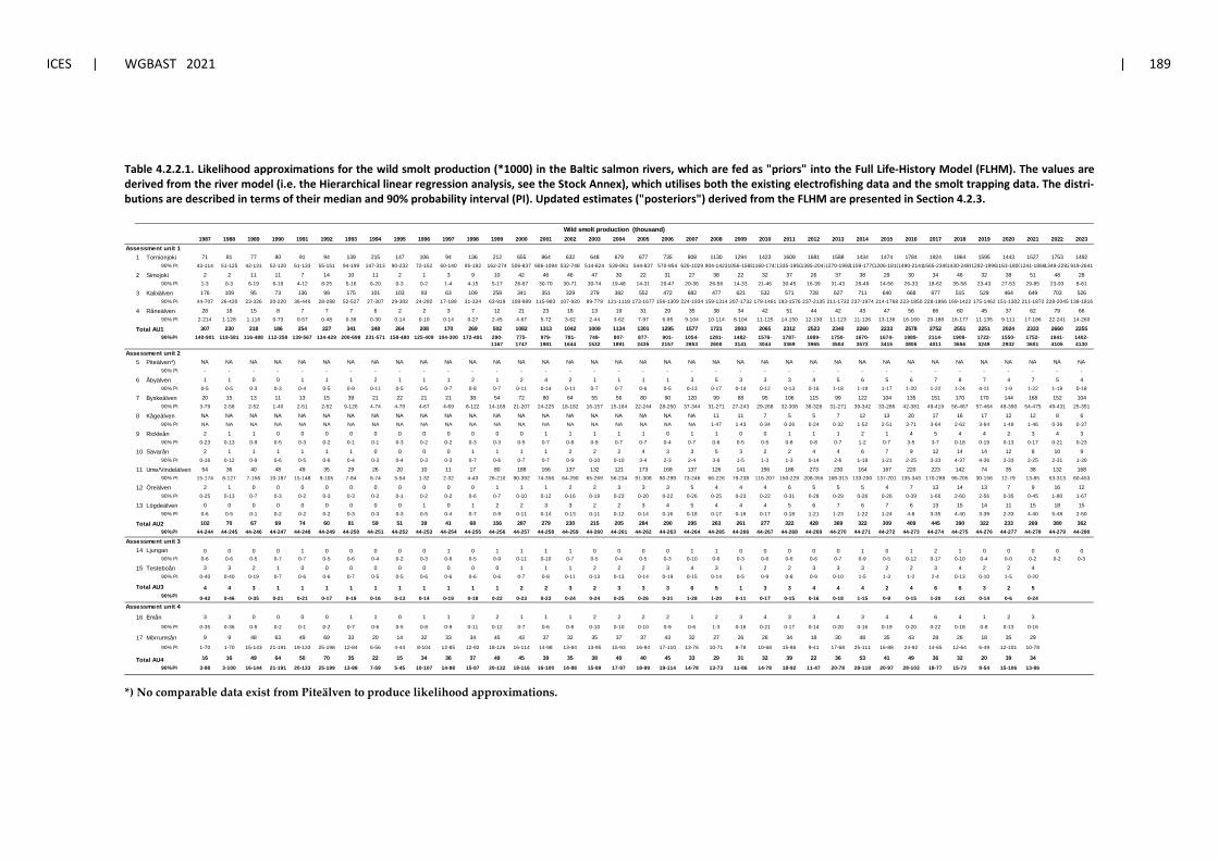
ICES | WGBAST 2021 | 189
Table 4.2.2.1. Likelihood approximations for the wild smolt production (*1000) in the Baltic salmon rivers, which are fed as "priors" into the Full Life-History Model (FLHM). The values are derived from the river model (i.e. the Hierarchical linear regression analysis, see the Stock Annex), which utilises both the existing electrofishing data and the smolt trapping data. The distri-butions are described in terms of their median and 90% probability interval (PI). Updated estimates ("posteriors") derived from the FLHM are presented in Section 4.2.3.
*) No comparable data exist from Piteälven to produce likelihood approximations.
1987 1988 1989 1990 1991 1992 1993 1994 1995 1996 1997 1998 1999 2000 2001 2002 2003 2004 2005 2006 2007 2008 2009 2010 2011 2012 2013 2014 2015 2016 2017 2018 2019 2020 2021 2022 2023
1 71 81 77 80 91 94 139 215 147 106 94 136 212 655 864 632 648 679 677 735 808 1130 1294 1423 1609 1681 1588 1434 1474 1784 1924 1864 1595 1443 1527 1753 149290% PI 43-114 51-125 42-131 52-120 61-133 55-151 94-199 147-313 90-232 72-152 60-140 95-192 162-274 506-837 686-1094 532-748 514-824 539-861 544-837 570-954 626-1029 904-14231056-15881160-17411335-19501385-20471270-19921159-17701206-18101490-21411565-23461430-24881292-19961163-18001241-18661349-2292919-2641
2 2 2 11 11 7 14 10 11 2 1 3 9 10 42 46 46 47 30 22 31 27 38 22 32 37 26 37 38 29 30 34 46 32 38 51 48 2890% PI 1-3 0-3 6-19 6-19 4-12 8-25 5-16 6-20 0-3 0-2 1-4 4-15 5-17 26-67 30-70 30-71 30-74 19-48 14-31 20-47 20-36 26-56 14-33 21-46 30-45 16-39 31-43 29-49 14-56 26-33 18-62 35-58 23-43 27-53 29-85 23-93 8-81
3 176 109 95 73 136 99 175 101 103 93 63 109 258 341 351 329 279 382 552 472 682 477 621 532 571 728 627 711 640 668 677 515 529 464 649 703 52690% PI 44-707 26-420 23-326 20-220 36-440 28-288 52-527 27-307 29-302 24-292 17-189 31-324 63-919 108-989 115-983 107-920 89-779 121-1118 173-1677 156-1309 224-1934 159-1314 207-1732 179-1461 193-1576 237-2135 211-1732 237-1974 214-1768 223-1850 228-1866 169-1422 175-1462 151-1302 211-1872 228-2045 138-1816
4 28 18 15 8 7 7 7 6 2 2 3 7 12 21 23 18 13 19 31 29 35 38 34 42 51 44 42 43 47 56 66 60 45 37 62 79 6690% PI 2-214 1-128 1-116 0-73 0-57 0-48 0-36 0-30 0-14 0-10 0-14 0-27 2-45 4-67 5-72 3-62 2-44 3-62 7-97 6-95 9-104 10-114 8-104 11-125 14-150 12-130 11-123 11-126 13-136 16-160 20-188 16-177 11-135 9-111 17-186 22-241 14-260
307 230 218 186 254 227 341 348 264 208 170 269 502 1082 1313 1042 1009 1134 1301 1295 1577 1721 2003 2065 2312 2523 2340 2260 2233 2578 2752 2551 2251 2024 2333 2660 225590% PI 140-901 119-581 116-488 112-358 139-567 134-429 200-698 231-571 158-480 125-409 104-300 172-491 290-
1167775-1747
979-1981
781-1644
749-1532
807-1891
877-2435
901-2157
1054-2853
1281-2600
1482-3141
1576-3044
1787-3369
1889-3965
1750-3504
1670-3572
1674-3415
1989-3805
2114-4011
1908-3656
1722-3249
1550-2932
1752-3601
1941-4105
1402-4130
5 NA NA NA NA NA NA NA NA NA NA NA NA NA NA NA NA NA NA NA NA NA NA NA NA NA NA NA NA NA NA NA NA NA NA NA NA NA90% PI - - - - - - - - - - - - - - - - - - - - - - - - - - - - - - - - - - - - -
6 1 1 0 0 1 1 1 2 1 1 1 2 1 2 4 2 1 1 1 1 3 5 3 3 3 4 5 6 5 6 7 8 7 4 7 5 490% PI 0-5 0-5 0-3 0-3 0-4 0-5 0-9 0-11 0-5 0-5 0-7 0-8 0-7 0-11 0-14 0-11 0-7 0-7 0-6 0-5 0-13 0-17 0-14 0-12 0-13 0-16 1-18 1-19 1-17 1-20 1-22 1-24 4-11 1-9 1-22 1-19 0-18
7 20 15 13 11 13 15 39 21 22 21 21 38 54 72 80 64 55 56 80 90 120 99 88 95 106 115 99 122 104 135 151 170 170 144 168 152 10490% PI 3-79 2-58 2-52 1-40 2-51 2-52 9-126 4-74 4-70 4-67 4-69 8-122 14-169 21-207 24-225 18-182 16-157 15-164 22-244 28-250 37-344 31-271 27-243 29-268 32-308 36-328 31-271 39-342 33-286 42-381 49-419 56-467 57-464 48-390 54-475 49-431 25-351
8 NA NA NA NA NA NA NA NA NA NA NA NA NA NA NA NA NA NA NA NA NA 11 11 7 5 5 7 12 13 20 17 16 17 12 12 8 690% PI NA NA NA NA NA NA NA NA NA NA NA NA NA NA NA NA NA NA NA NA NA 1-47 1-43 0-34 0-26 0-24 0-32 1-52 2-51 3-71 3-64 2-62 3-64 1-49 1-46 0-36 0-37
9 2 1 1 0 0 0 0 0 0 0 0 0 0 0 1 1 1 1 1 0 1 1 0 0 1 1 1 2 1 4 5 4 4 2 3 4 390% PI 0-23 0-13 0-9 0-5 0-3 0-2 0-1 0-1 0-3 0-2 0-2 0-3 0-3 0-5 0-7 0-8 0-9 0-7 0-7 0-4 0-7 0-6 0-5 0-5 0-8 0-8 0-7 1-2 0-7 3-5 3-7 0-18 0-19 0-13 0-17 0-21 0-23
10 2 1 1 1 1 1 1 0 0 0 0 1 1 1 1 2 2 2 4 3 3 5 3 2 2 4 4 6 7 9 12 14 14 12 8 10 990% PI 0-16 0-12 0-9 0-6 0-5 0-6 0-4 0-3 0-4 0-3 0-3 0-7 0-6 0-7 0-7 0-9 0-10 0-10 3-4 2-3 2-4 3-6 1-5 1-3 1-3 0-14 2-6 1-18 1-21 2-25 3-33 4-37 4-36 3-33 2-25 2-31 1-30
11 54 36 40 48 49 35 29 26 20 10 11 17 80 188 166 137 132 121 173 168 137 126 141 156 186 273 230 164 167 220 223 142 74 35 38 132 16890% PI 15-174 8-127 7-156 10-187 15-148 9-105 7-84 6-74 5-54 1-32 2-32 4-43 26-210 90-392 74-356 64-290 65-269 56-234 91-308 90-299 73-246 66-226 79-238 116-207 150-229 208-355 168-313 133-200 137-201 135-343 170-289 96-205 30-156 12-79 13-85 53-313 60-453
12 2 1 0 0 0 0 0 0 0 0 0 0 1 1 1 2 2 3 3 3 5 4 4 4 6 5 5 5 4 7 13 14 13 7 9 16 1290% PI 0-25 0-13 0-7 0-3 0-2 0-3 0-3 0-2 0-1 0-2 0-2 0-6 0-7 0-10 0-12 0-16 0-19 0-23 0-20 0-22 0-26 0-25 0-23 0-22 0-31 0-28 0-29 0-26 0-26 0-39 1-60 2-60 2-56 0-35 0-45 1-80 1-67
13 0 0 0 0 0 0 0 0 0 1 0 1 2 2 3 3 2 2 3 4 5 4 4 4 5 6 7 6 7 6 13 15 14 11 15 18 1590% PI 0-6 0-5 0-1 0-2 0-2 0-2 0-3 0-3 0-3 0-5 0-4 0-7 0-9 0-11 0-14 0-13 0-11 0-12 0-14 0-16 0-18 0-17 0-16 0-17 0-18 1-21 1-23 1-22 1-24 4-8 3-35 4-40 3-39 2-33 4-40 5-48 2-50
102 70 67 69 74 60 81 59 51 39 41 68 156 287 279 230 215 205 284 290 295 263 261 277 322 428 369 322 309 409 445 390 322 233 269 380 36290% PI 44-244 44-245 44-246 44-247 44-248 44-249 44-250 44-251 44-252 44-253 44-254 44-255 44-256 44-257 44-258 44-259 44-260 44-261 44-262 44-263 44-264 44-265 44-266 44-267 44-268 44-269 44-270 44-271 44-272 44-273 44-274 44-275 44-276 44-277 44-278 44-279 44-280
14 0 0 0 0 1 0 0 0 0 0 1 0 1 1 1 1 0 0 0 0 1 1 0 0 0 0 0 1 0 1 2 1 0 0 0 0 090% PI 0-6 0-6 0-5 0-7 0-7 0-5 0-6 0-4 0-2 0-3 0-6 0-5 0-9 0-11 0-10 0-7 0-5 0-4 0-5 0-3 0-10 0-6 0-3 0-6 0-6 0-6 0-7 0-9 0-5 0-12 0-17 0-10 0-4 0-0 0-2 0-2 0-3
15 3 3 2 1 0 0 0 0 0 0 0 0 0 1 1 1 2 2 2 3 4 3 1 2 2 3 3 3 2 2 3 4 2 2 490% PI 0-40 0-40 0-19 0-7 0-6 0-6 0-7 0-5 0-5 0-6 0-6 0-6 0-6 0-7 0-8 0-11 0-13 0-13 0-14 0-19 0-15 0-14 0-5 0-9 0-8 0-9 0-10 1-5 1-3 1-2 2-4 0-13 0-10 1-5 0-20
4 4 3 1 1 1 1 1 1 1 1 1 1 2 2 3 2 3 3 3 6 5 1 3 3 4 4 4 2 4 6 6 3 2 590% PI 0-42 0-46 0-35 0-21 0-21 0-17 0-19 0-16 0-13 0-14 0-19 0-18 0-22 0-23 0-23 0-24 0-24 0-25 0-26 0-31 1-28 1-20 0-11 0-17 0-15 0-16 0-18 1-15 0-9 0-15 1-20 1-21 0-14 0-6 0-24
16 3 3 0 0 0 0 1 1 0 1 1 2 2 1 1 1 2 2 2 2 1 2 3 4 3 3 4 3 4 4 6 4 1 2 3
90% PI 0-35 0-36 0-5 0-2 0-1 0-2 0-7 0-6 0-5 0-8 0-9 0-11 0-12 0-7 0-6 0-8 0-10 0-10 0-10 0-9 0-6 1-3 0-16 0-21 0-17 0-14 0-20 0-16 0-19 0-20 0-22 0-18 0-8 0-13 0-16
17 9 9 48 63 49 69 33 20 14 32 33 34 45 43 37 32 35 37 37 43 32 27 26 26 34 18 30 48 35 43 28 26 18 35 29
90% PI 1-70 1-70 15-143 21-191 19-133 25-198 12-84 6-56 4-44 8-104 12-85 12-92 18-126 16-114 14-98 13-84 13-95 15-93 16-94 17-110 13-76 10-71 8-78 10-68 15-86 9-41 17-68 25-111 16-88 24-92 14-65 12-64 6-49 12-101 10-78
16 16 49 64 50 70 35 22 15 34 36 37 49 45 39 35 38 40 40 45 33 29 31 32 39 22 36 53 41 49 36 32 20 39 3490% PI 3-98 3-100 16-144 21-191 20-133 25-199 13-88 7-59 5-45 10-107 14-88 15-97 20-132 18-116 16-100 14-88 15-99 17-97 18-99 19-114 14-78 13-73 11-86 14-78 18-92 11-47 20-78 28-118 20-97 28-103 18-77 15-73 8-54 15-106 13-86
Assessment unit 1
Assessment unit 2
Assessment unit 3
Total AU4
Ume/Vindelälven
Lögdeälven
Total AU3
Ljungan
Total AU2
Emån
Mörrumsån
Assessment unit 4
Testeboån
Byskeälven
Kågeälven
Rickleån
Sävarån
Tornionjoki
Simojoki
Kalixälven
Råneälven
Öreälven
Wild smolt production (thousand)
Piteälven*)
Åbyälven
Total AU1
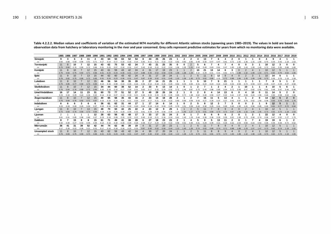
190 | ICES SCIENTIFIC REPORTS 3:26 | ICES
Table 4.2.2.2. Median values and coefficients of variation of the estimated M74 mortality for different Atlantic salmon stocks (spawning years 1985–2019). The values in bold are based on observation data from hatchery or laboratory monitoring in the river and year concerned. Grey cells represent predictive estimates for years from which no monitoring data were available.
1985 1986 1987 1988 1989 1990 1991 1992 1993 1994 1995 1996 1997 1998 1999 2000 2001 2002 2003 2004 2005 2006 2007 2008 2009 2010 2011 2012 2013 2014 2015 2016 2017 2018 2019Simojoki 9 3 6 3 11 4 43 64 50 63 52 54 8 44 25 26 23 1 2 2 4 13 7 6 4 2 0 1 1 0 4 9 4 1 1 cv 0.60 0.88 0.58 0.96 0.51 0.71 0.17 0.14 0.17 0.10 0.16 0.14 0.30 0.11 0.21 0.22 0.22 0.62 0.60 0.90 0.49 0.30 0.47 0.47 0.61 0.72 1.92 1.36 1.15 1.60 0.70 0.33 0.42 1.19 1.63Tornionjoki 11 8 10 7 12 15 43 62 75 53 42 24 7 43 21 25 35 0 0 2 5 6 7 4 7 4 0 0 3 1 10 12 3 0 0 cv 0.75 0.84 0.76 0.90 0.72 0.66 0.31 0.25 0.07 0.10 0.31 0.47 0.43 0.18 0.22 0.22 0.24 1.06 1.39 1.31 0.50 0.49 0.63 0.61 0.47 1.00 1.99 1.43 1.09 1.45 0.72 0.63 0.35 0.88 1.80Kemijoki 11 8 10 7 12 15 43 61 59 43 42 24 4 31 17 19 23 1 1 2 10 21 13 14 6 3 0 2 4 1 10 12 5 1 1 cv 0.76 0.83 0.75 0.92 0.71 0.66 0.31 0.24 0.23 0.30 0.31 0.47 0.88 0.40 0.52 0.50 0.45 1.09 1.38 1.28 0.32 0.29 0.41 0.31 0.52 0.71 1.88 1.32 1.09 1.44 0.71 0.62 0.75 0.63 1.65Iijoki 11 9 10 7 13 15 44 62 60 43 42 24 4 31 17 19 24 1 1 2 5 11 8 12 9 4 0 2 3 1 10 14 5 1 1 cv 0.76 0.82 0.75 0.90 0.72 0.65 0.31 0.24 0.23 0.30 0.31 0.47 0.87 0.39 0.52 0.51 0.45 1.10 1.39 1.30 0.73 0.62 0.80 0.33 0.72 0.99 1.84 1.35 1.09 1.46 0.73 0.35 0.76 1.19 1.59Luleälven 11 8 10 7 12 15 46 56 54 38 35 28 2 27 14 21 25 1 1 1 5 10 7 9 21 1 1 1 1 1 7 8 5 1 2 cv 0.75 0.85 0.77 0.90 0.73 0.65 0.13 0.16 0.08 0.13 0.20 0.16 0.36 0.12 0.18 0.15 0.20 0.62 0.43 0.65 0.41 0.24 0.24 0.22 0.20 0.42 0.58 0.74 0.59 0.57 0.39 0.47 0.44 0.47 0.58Skellelteälven 11 8 10 7 12 15 34 44 60 38 52 14 2 33 9 13 14 1 0 1 2 7 1 2 4 2 1 10 1 1 4 10 5 6 1 cv 0.76 0.84 0.76 0.89 0.72 0.66 0.20 0.18 0.10 0.17 0.20 0.31 0.63 0.17 0.32 0.29 0.32 0.72 1.46 0.87 0.70 0.40 0.88 0.80 0.54 0.72 0.99 0.47 0.82 0.91 0.61 0.49 0.47 0.44 0.98Ume/Vindelälven 16 17 14 11 23 31 60 73 77 51 52 27 5 40 28 26 24 2 1 0 2 8 4 14 13 6 0 4 10 0 11 14 5 2 0 cv 0.23 0.33 0.29 0.43 0.26 0.32 0.14 0.16 0.07 0.13 0.19 0.21 0.45 0.15 0.20 0.19 0.25 0.65 0.72 1.38 0.62 0.40 0.55 0.27 0.32 0.41 1.97 0.56 0.43 1.55 0.46 0.50 0.58 0.63 1.66Ångermanälven 11 8 10 7 12 15 40 65 58 35 43 16 2 23 14 18 28 2 1 2 7 15 11 5 13 4 1 1 2 0 14 12 5 2 0 cv 0.75 0.84 0.76 0.92 0.71 0.67 0.15 0.16 0.10 0.16 0.21 0.20 0.57 0.17 0.21 0.19 0.22 0.60 0.56 0.59 0.43 0.27 0.28 0.37 0.27 0.42 0.97 0.75 0.62 1.50 0.39 0.63 0.75 0.63 1.76Indalsälven 6 6 6 3 6 6 36 61 62 31 44 17 1 17 14 6 14 1 0 2 5 8 12 3 7 3 0 0 2 1 9 12 5 1 1 cv 0.23 0.33 0.29 0.45 0.30 0.37 0.15 0.16 0.08 0.15 0.20 0.20 0.64 0.19 0.22 0.33 0.25 0.70 1.51 0.59 0.44 0.30 0.25 0.41 0.30 0.40 1.95 1.41 0.56 0.65 0.40 0.61 0.77 0.72 0.94Ljungan 11 8 10 7 13 15 48 70 50 42 25 22 4 23 12 9 29 1 1 2 5 11 7 8 9 4 0 2 4 1 10 12 5 1 1 cv 0.75 0.83 0.76 0.90 0.72 0.66 0.19 0.20 0.20 0.19 0.30 0.32 0.61 0.29 0.49 0.56 0.30 1.14 1.40 1.27 0.73 0.61 0.80 0.73 0.72 0.97 1.85 1.32 1.06 1.45 0.73 0.62 0.75 1.18 1.63Ljusnan 2 1 1 1 1 12 28 63 56 42 48 17 3 33 17 31 24 2 0 1 7 8 6 9 6 2 0 1 2 1 22 12 4 0 0 cv 0.81 0.91 0.85 0.98 0.80 0.37 0.19 0.16 0.09 0.15 0.20 0.22 0.45 0.18 0.21 0.16 0.24 0.61 1.43 1.29 0.44 0.36 0.36 0.28 0.35 0.52 1.98 0.75 0.58 0.74 0.36 0.47 0.52 1.27 1.70Dalälven 8 7 15 8 8 15 61 71 49 41 39 28 6 27 18 23 23 2 1 4 5 9 5 13 11 2 0 1 7 4 19 19 6 1 2 cv 0.42 0.40 0.27 0.42 0.45 0.35 0.14 0.16 0.10 0.18 0.20 0.18 0.38 0.17 0.20 0.19 0.22 0.58 0.52 0.45 0.41 0.29 0.35 0.21 0.26 0.42 2.03 0.66 0.44 0.53 0.36 0.45 0.44 0.72 0.62Mörrumsån 36 41 31 39 52 42 44 74 62 46 39 19 4 31 17 20 23 1 1 2 5 11 7 8 9 4 0 2 4 1 10 12 5 1 1 cv 0.17 0.28 0.22 0.28 0.21 0.31 0.17 0.16 0.18 0.18 0.25 0.33 0.87 0.40 0.52 0.50 0.44 1.13 1.40 1.26 0.74 0.62 0.80 0.74 0.71 0.98 1.88 1.33 1.07 1.47 0.73 0.62 0.74 1.19 1.62Unsampled stock 11 8 10 7 12 15 43 62 59 43 42 24 4 30 17 20 24 1 1 2 5 11 8 8 9 4 0 2 4 1 10 12 5 1 1 cv 0.76 0.83 0.75 0.90 0.72 0.66 0.31 0.24 0.23 0.30 0.31 0.47 0.87 0.40 0.52 0.50 0.44 1.12 1.38 1.23 0.74 0.61 0.81 0.73 0.72 1.00 1.88 1.32 1.08 1.45 0.73 0.62 0.74 1.18 1.65
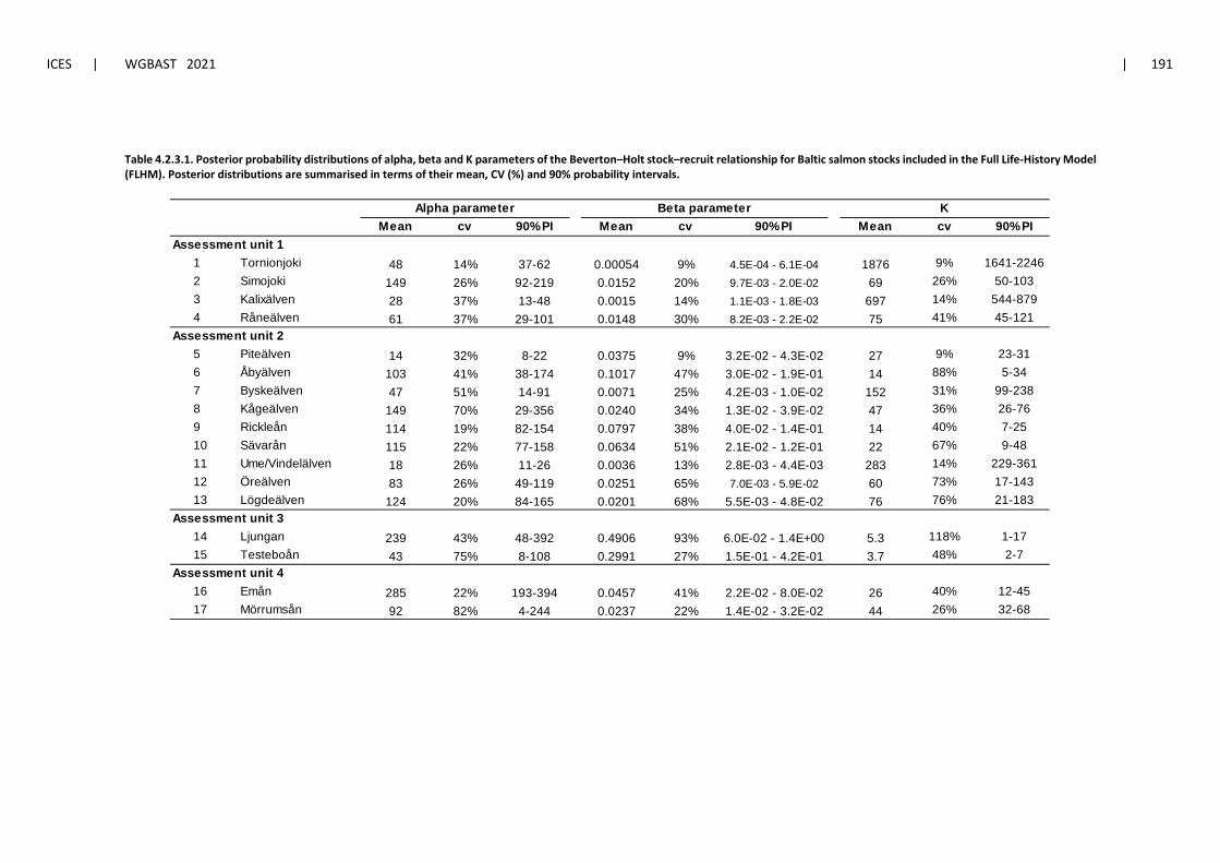
ICES | WGBAST 2021 | 191
Table 4.2.3.1. Posterior probability distributions of alpha, beta and K parameters of the Beverton–Holt stock–recruit relationship for Baltic salmon stocks included in the Full Life-History Model (FLHM). Posterior distributions are summarised in terms of their mean, CV (%) and 90% probability intervals.
Mean cv 90% PI Mean cv 90% PI Mean cv 90% PI
1 Tornionjoki 48 14% 37-62 0.00054 9% 4.5E-04 - 6.1E-04 1876 9% 1641-22462 Simojoki 149 26% 92-219 0.0152 20% 9.7E-03 - 2.0E-02 69 26% 50-1033 Kalixälven 28 37% 13-48 0.0015 14% 1.1E-03 - 1.8E-03 697 14% 544-8794 Råneälven 61 37% 29-101 0.0148 30% 8.2E-03 - 2.2E-02 75 41% 45-121
5 Piteälven 14 32% 8-22 0.0375 9% 3.2E-02 - 4.3E-02 27 9% 23-316 Åbyälven 103 41% 38-174 0.1017 47% 3.0E-02 - 1.9E-01 14 88% 5-347 Byskeälven 47 51% 14-91 0.0071 25% 4.2E-03 - 1.0E-02 152 31% 99-2388 Kågeälven 149 70% 29-356 0.0240 34% 1.3E-02 - 3.9E-02 47 36% 26-769 Rickleån 114 19% 82-154 0.0797 38% 4.0E-02 - 1.4E-01 14 40% 7-2510 Sävarån 115 22% 77-158 0.0634 51% 2.1E-02 - 1.2E-01 22 67% 9-4811 Ume/Vindelälven 18 26% 11-26 0.0036 13% 2.8E-03 - 4.4E-03 283 14% 229-36112 Öreälven 83 26% 49-119 0.0251 65% 7.0E-03 - 5.9E-02 60 73% 17-14313 Lögdeälven 124 20% 84-165 0.0201 68% 5.5E-03 - 4.8E-02 76 76% 21-183
14 Ljungan 239 43% 48-392 0.4906 93% 6.0E-02 - 1.4E+00 5.3 118% 1-1715 Testeboån 43 75% 8-108 0.2991 27% 1.5E-01 - 4.2E-01 3.7 48% 2-7
16 Emån 285 22% 193-394 0.0457 41% 2.2E-02 - 8.0E-02 26 40% 12-4517 Mörrumsån 92 82% 4-244 0.0237 22% 1.4E-02 - 3.2E-02 44 26% 32-68
Assessment unit 4
Assessment unit 1
Assessment unit 2
KAlpha parameter Beta parameter
Assessment unit 3
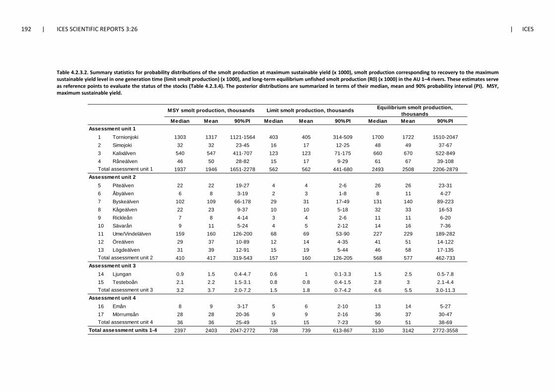
192 | ICES SCIENTIFIC REPORTS 3:26 | ICES
Table 4.2.3.2. Summary statistics for probability distributions of the smolt production at maximum sustainable yield (x 1000), smolt production corresponding to recovery to the maximum sustainable yield level in one generation time (limit smolt production) (x 1000), and long-term equilibrium unfished smolt production (R0) (x 1000) in the AU 1–4 rivers. These estimates serve as reference points to evaluate the status of the stocks (Table 4.2.3.4). The posterior distributions are summarized in terms of their median, mean and 90% probability interval (PI). MSY, maximum sustainable yield.
Median Mean 90% PI Median Mean 90% PI Median Mean 90% PI
1 Tornionjoki 1303 1317 1121-1564 403 405 314-509 1700 1722 1510-20472 Simojoki 32 32 23-45 16 17 12-25 48 49 37-673 Kalixälven 540 547 411-707 123 123 71-175 660 670 522-8494 Råneälven 46 50 28-82 15 17 9-29 61 67 39-108
1937 1946 1651-2278 562 562 441-680 2493 2508 2206-2879
5 Piteälven 22 22 19-27 4 4 2-6 26 26 23-316 Åbyälven 6 8 3-19 2 3 1-8 8 11 4-277 Byskeälven 102 109 66-178 29 31 17-49 131 140 89-2238 Kågeälven 22 23 9-37 10 10 5-18 32 33 16-539 Rickleån 7 8 4-14 3 4 2-6 11 11 6-2010 Sävarån 9 11 5-24 4 5 2-12 14 16 7-3611 Ume/Vindelälven 159 160 126-200 68 69 53-90 227 229 189-28212 Öreälven 29 37 10-89 12 14 4-35 41 51 14-12213 Lögdeälven 31 39 12-91 15 19 5-44 46 58 17-135
410 417 319-543 157 160 126-205 568 577 462-733
14 Ljungan 0.9 1.5 0.4-4.7 0.6 1 0.1-3.3 1.5 2.5 0.5-7.815 Testeboån 2.1 2.2 1.5-3.1 0.8 0.8 0.4-1.5 2.8 3 2.1-4.4
3.2 3.7 2.0-7.2 1.5 1.8 0.7-4.2 4.6 5.5 3.0-11.3
16 Emån 8 9 3-17 5 6 2-10 13 14 5-2717 Mörrumsån 28 28 20-36 9 9 2-16 36 37 30-47
36 36 25-49 15 15 7-23 50 51 38-692397 2403 2047-2772 738 739 613-867 3130 3142 2772-3558
Total assessment unit 4Total assessment units 1-4
Assessment unit 3
Assessment unit 2
Total assessment unit 2
MSY smolt production, thousands
Total assessment unit 3Assessment unit 4
Limit smolt production, thousands Equilibrium smolt production, thousands
Assessment unit 1
Total assessment unit 1
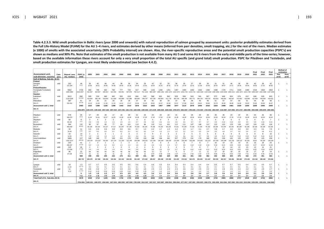
ICES | WGBAST 2021 | 193
Table 4.2.3.3. Wild smolt production in Baltic rivers (year 2000 and onwards) with natural reproduction of salmon grouped by assessment units: posterior probability estimates derived from the Full Life-History Model (FLHM) for the AU 1–4 rivers, and estimates derived by other means (inferred from parr densities, smolt trapping, etc.) for the rest of the rivers. Median estimates (x 1000) of smolts with the associated uncertainty (90% Probability interval) are shown. Also, the river-specific reproductive areas and the potential smolt production capacities (PSPC's) are shown as medians and 90% PIs. Note that estimates of the smolt production is not available from many AU 5 and some AU 6 rivers from the early and middle parts of the time-series; however, based on the available information these rivers account for only a very small proportion of the total AU specific (and grand total) smolt production. PSPC for Piteälven and Testeboån, and smolt production estimates for Ljungan, are most likely underestimated (see Section 4.4.2).
Pred Pred Pred2000 2001 2002 2003 2004 2005 2006 2007 2008 2009 2010 2011 2012 2013 2014 2015 2016 2017 2018 2019 2020 2021 2022 2023 Pot. Pres.
prod. prod.Gulf of Bothnia, Sub-div. 30-31:FinlandSimojoki wild 252 48 26 40 46 44 38 30 34 29 42 32 33 36 30 37 38 35 31 51 46 36 38 40 38 42 1 190% PI 222-284 37-67 18-36 30-51 35-60 34-58 29-50 23-39 26-45 23-36 33-54 25-42 26-42 31-43 23-40 32-43 31-48 25-49 28-35 38-67 37-57 29-45 30-49 30-55 27-52 30-60Finland/SwedenTornionjoki;Torneälven wild 5562 1700 680 795 692 765 777 728 917 909 1163 1260 1251 1357 1465 1450 1363 1360 1598 1725 1711 1549 1485 1533 1663 1653 1 190% PI 4405-6985 1510-2047 561-827 653-947 595-813 621-930 634-951 607-876 750-1117 751-1103 980-1397 1055-1491 1051-1473 1154-1575 1256-1732 1218-1721 1160-1620 1133-1618 1365-1856 1443-2040 1393-2111 1282-1872 1225-1769 1298-1837 1352-2060 1197-2259SwedenKalixälven wild 2612 660 585 534 460 462 593 618 684 543 568 631 562 539 568 543 541 567 572 648 654 676 612 626 628 643 1 190% PI 2129-3208 522-849 415-804 385-738 320-654 317-658 403-888 427-886 484-963 390-767 407-790 440-903 411-778 383-740 408-789 392-772 384-755 400-787 403-816 460-891 460-937 473-952 426-886 427-904 436-930 429-921Råneälven wild 387 61 24 28 21 20 25 29 37 33 42 38 34 37 40 44 43 45 51 57 57 54 51 54 56 59 1 190% PI 333-451 39-108 13-43 15-48 11-36 11-34 14-41 17-47 23-56 21-49 28-62 24-57 22-55 24-57 27-60 29-67 28-64 30-66 33-78 36-90 36-89 34-86 33-83 34-85 35-90 36-97Assessment unit 1, total 2493 1323 1398 1226 1298 1443 1410 1676 1523 1833 1967 1898 1977 2110 2078 2006 2016 2264 2498 2481 2329 2200 2269 2405 2409 1 1
90% PI 2206-2879 1105-1575 1196-1643 1057-1442 1087-1533 1197-1766 1181-1716 1402-2036 1290-1819 1571-2139 1690-2320 1628-2186 1709-2270 1852-2467 1798-2435 1710-2307 1730-2353 1963-2597 2144-2887 2107-2956 1971-2737 1866-2596 1953-2668 2005-2876 1892-3081
Piteälven wild 576 26 17 29 28 17 19 20 21 23 23 24 22 21 22 26 26 26 26 26 24 24 25 25 25 26 1 190% PI 482-670 23-31 11-24 21-41 22-37 12-23 14-26 14-28 15-28 17-30 17-30 17-32 17-29 15-28 16-29 19-34 20-34 19-35 19-36 20-34 17-33 17-33 18-36 18-35 18-36 18-36Åbyälven wild 84 8 3 4 3 2 3 3 4 4 5 4 3 3 4 5 4 5 6 6 6 6 6 6 6 7 1 190% PI 69-102 4-27 2-6 2-8 1-5 1-5 1-5 1-5 2-7 2-6 3-8 2-6 2-6 2-6 2-6 3-7 3-7 3-7 4-9 4-10 4-10 5-9 4-9 4-9 4-10 4-13Byskeälven wild 564 131 95 97 85 77 93 101 113 96 115 111 101 112 111 107 106 112 123 133 125 128 122 124 125 126 1 190% PI 483-658 89-223 60-140 65-143 54-127 47-117 62-140 67-146 79-163 66-140 79-168 76-163 69-149 74-161 76-158 74-155 72-155 76-162 84-184 92-199 84-195 88-199 82-185 83-185 82-189 83-203Rickleån wild 34 11 0.3 0.9 0.9 0.8 0.8 0.6 0.7 1.0 2.2 1.7 1.3 1.2 1.2 1.7 2.1 2.7 3.8 4.7 4.2 3.6 3.9 4.3 5.1 7.0 1 190% PI 24-49 6-20 0-1 0-2 0-2 0-1 0-2 0-1 0-1 0-2 1-4 1-3 1-2 1-2 1-2 1-3 2-3 2-4 3-5 4-6 3-7 2-6 2-6 3-7 3-8 4-11Sävarån wild 23 14 2 3 2 1 2 4 3 3 5 3 3 3 4 5 4 5 6 8 9 8 8 8 8 10 1 190% PI 14-35 7-36 1-3 1-5 1-3 1-3 1-4 3-4 3-4 2-4 4-6 2-5 2-4 2-4 3-6 3-6 3-7 3-8 4-9 5-12 6-13 5-12 5-13 5-12 5-14 6-19Ume/Vindelälven wild 1806 227 185 160 77 139 151 176 216 193 186 194 181 207 279 231 170 180 221 238 181 153 125 53 125 208 1 190% PI 1432-2272 189-282 145-234 123-210 56-105 107-179 111-205 131-240 164-286 149-252 137-249 146-249 145-220 173-245 228-340 183-289 143-201 151-215 167-293 194-288 142-233 109-212 84-183 30-87 83-183 149-293Öreälven wild 244 41 1 2 1 1 1 2 3 3 4 3 3 3 5 7 6 7 10 14 15 14 15 15 18 23 1 190% PI 200-297 14-122 0-2 1-3 0-2 0-2 1-3 1-3 1-6 1-5 2-8 2-6 1-5 2-7 3-9 3-12 4-12 4-13 5-18 8-23 9-26 8-25 8-26 8-27 10-32 12-45Lögdeälven wild 210 46 2 3 2 1 2 3 4 4 5 3 3 4 5 7 6 7 7 12 14 13 13 13 14 2190% PI 172-256 17-135 1-5 1-6 1-3 1-3 1-4 1-6 2-8 2-6 3-8 2-6 2-5 2-7 3-9 4-11 4-10 4-11 5-10 8-19 9-23 8-22 8-22 8-22 '9-23 13-35Kågeälven wild 96 32 na na na na na na na na 12 11 7 5 5 7 11 11 17 20 18 16 16 17 19 24 1 190% PI 67-138 16-53 na na na na na na na na 3-57 3-49 1-30 1-27 1-23 2-32 3-37 3-37 5-66 9-36 8-32 7-30 7-31 8-33 9-35 12-43Assessment unit 2, total 568 308 302 200 242 276 311 369 331 367 363 329 365 441 401 343 362 432 468 403 375 342 272 351 464 1 1
90% PI 462-733 249-378 247-368 156-250 193-304 221-343 249-391 301-449 270-402 299-457 295-448 276-395 315-430 376-522 340-478 293-404 311-427 355-535 402-557 340-494 308-460 275-430 216-342 286-440 378-584
Ljungan wild 19 1.5 0.7 0.7 0.5 0.5 0.5 0.5 0.6 0.4 0.6 0.5 0.4 0.4 0.4 0.4 0.4 0.4 0.5 0.7 0.7 0.5 0.4 0.4 0.5 0.7 1 190% PI 11-34 0,5-7,8 0-2 0-2 0-1 0-1 0-1 0-1 0-1 0-1 0-1 0-1 0-1 0-1 0-1 0-1 0-1 0-1 0-1 0-1 0-1 0-1 0-1 0-1 0-1 0-2Testeboån wild 11 2.8 0.6 0.9 1.7 2.2 2.0 2.4 3.3 3.8 2.5 2.2 2.3 2.3 2.6 2.4 2.5 2.2 2.1 2.8 2.5 2.3 2.4 1.6 2.9 2.7 1 190% PI 9-13 2,1-4,4 0-13 0-15 0-52 0-35 0-25 0-22 0-32 1-25 1-4 1-4 1-4 1-4 1-4 1-4 2-4 1-3 2-3 2-4 1-4 1-3 2-3 1-3 2-5 2-4Assessment unit 3, total 5 1.5 1.8 2.3 2.7 2.5 2.9 4.0 4.3 3.2 2.7 2.8 2.8 3.0 2.8 3.0 2.7 2.6 3.5 3.2 2.8 2.9 2.1 3.5 3.5 1 195% PI 3-11 0-14 1-16 1-53 1-35 1-26 1-22 1-33 1-25 2-5 1-4 1-4 1-4 2-5 2-4 2-4 2-4 2-3 3-5 2-5 2-4 2-4 1-3 2-5 2-5Total Gulf of B., Sub-divs.30-31 3078 1638 1712 1445 1554 1732 1734 2058 1860 2202 2335 2232 2346 2556 2491 2349 2380 2702 2965 2888 2707 2549 2547 2764 2882 1 1
90% PI 2726-3504 1400-1911 1490-1973 1264-1691 1327-1816 1482-2058 1487-2049 1782-2430 1612-2167 1937-2517 2047-2697 1959-2524 2080-2645 2277-2917 2197-2851 2055-2670 2082-2731 2381-3059 2613-3364 2507-3369 2351-3124 2210-2944 2226-2951 2355-3251 2344-3568
Cate-gory
estimationMethod of
PSPC (x 1000)
Reprod. area (ha, median)
Assessment unit, sub-division, country
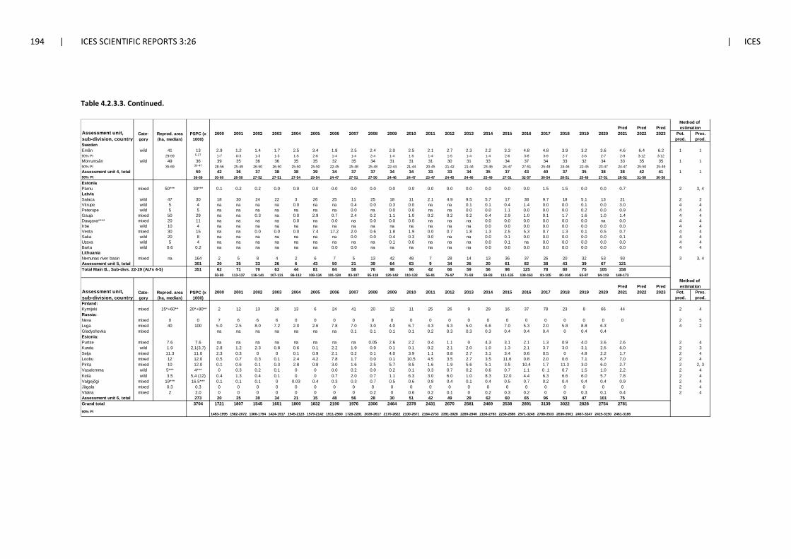
194 | ICES SCIENTIFIC REPORTS 3:26 | ICES
Table 4.2.3.3. Continued.
Pred Pred Pred2000 2001 2002 2003 2004 2005 2006 2007 2008 2009 2010 2011 2012 2013 2014 2015 2016 2017 2018 2019 2020 2021 2022 2023 Pot. Pres.
prod. prod.SwedenEmån wild 41 13 2.9 1.2 1.4 1.7 2.5 3.4 1.8 2.5 2.4 2.0 2.5 2.1 2.7 2.3 2.2 3.3 4.8 4.8 3.9 3.2 3.6 4.6 6.4 6.2 1 190% PI 29-59 5-27 1-7 0-3 1-3 1-3 1-5 2-6 1-4 1-4 2-4 1-4 1-5 1-4 1-5 1-4 1-4 2-6 3-8 3-9 2-7 2-6 2-7 2-9 3-12 3-12Mörrumsån wild 49 36 39 35 36 36 35 35 32 35 34 31 31 31 30 31 33 34 37 34 33 32 34 33 35 35 1 190% PI 35-69 30-47 28-56 25-49 26-50 26-50 25-50 25-50 22-45 25-48 25-48 22-44 21-44 20-45 21-42 21-44 23-46 24-47 27-51 25-48 24-46 22-45 23-47 24-47 25-50 25-49Assessment unit 4, total 50 42 36 37 38 38 39 34 37 37 34 34 33 33 34 35 37 43 40 37 35 38 38 42 41 1 190% PI 38-69 30-60 26-50 27-52 27-51 27-54 29-54 24-47 27-51 27-50 24-46 24-47 23-47 24-45 24-46 25-49 27-51 32-57 30-54 28-51 25-49 27-51 28-52 31-58 30-58EstoniaPärnu mixed 50*** 30*** 0.1 0.2 0.2 0.0 0.0 0.0 0.0 0.0 0.0 0.0 0.0 0.0 0.0 0.0 0.0 0.0 0.0 1.5 1.5 0.0 0.0 0.7 2 3, 4LatviaSalaca wild 47 30 18 30 24 22 3 26 25 11 25 18 11 2.1 4.9 9.5 5.7 17 38 9.7 18 5.1 13 21 2 2Vitrupe wild 5 4 na na na na 0.0 na na 0.4 0.0 0.3 0.0 na na 0.1 0.1 0.4 1.4 0.0 0.0 0.1 0.0 3.0 4 4Peterupe wild 5 5 na na na na na na na 0.0 na 0.0 0.0 na na 0.0 0.0 1.1 0.0 0.0 0.0 0.2 0.0 0.9 4 4Gauja mixed 50 29 na na 0.3 na 0.0 2.9 0.7 2.4 0.2 1.1 1.0 0.2 0.2 0.2 0.4 2.9 1.0 0.1 1.7 1.6 1.0 1.4 4 4Daugava**** mixed 20 11 na na na na 0.0 na 0.0 na 0.0 0.0 0.0 na na na 0.0 0.0 0.0 0.0 0.0 0.0 na 0.0 4 4Irbe wild 10 4 na na na na na na na na na na na na na na 0.0 0.0 0.0 0.0 0.0 0.0 0.0 0.0 4 4Venta mixed 30 15 na na 0.0 0.0 0.0 7.4 17.2 2.0 0.6 1.8 1.9 0.0 0.7 1.8 1.3 2.5 5.3 0.7 1.3 0.1 0.5 0.7 4 4Saka wild 20 8 na na na na na na na 0.0 0.0 0.4 0.3 0.0 na na 0.0 0.1 0.0 0.0 0.0 0.0 0.0 0.1 4 4Uzava wild 5 4 na na na na na na na na na 0.1 0.0 na na na 0.0 0.1 na 0.0 0.0 0.0 0.0 0.0 4 4Barta wild 0.6 0.2 na na na na na na 0.0 0.0 na na na na na na 0.0 0.0 0.0 0.0 0.0 0.0 0.0 0.0 4 4LithuaniaNemunas river basin mixed na 164 2 5 8 4 2 6 7 5 13 42 48 7 28 14 13 36 37 26 20 32 53 93 3 3, 4Assessment unit 5, total 301 20 35 33 26 6 43 50 21 39 64 63 9 34 26 20 61 82 38 43 39 67 121Total Main B., Sub-divs. 22-29 (AU's 4-5) 351 62 71 70 63 44 81 84 58 76 98 96 42 66 59 56 98 125 78 80 75 105 158
50-80 113-137 116-141 107-131 86-112 108-134 101-124 83-107 95-118 120-142 110-133 56-81 76-97 71-93 59-83 111-135 138-163 81-105 80-104 63-87 94-119 149-173
Pred Pred Pred2000 2001 2002 2003 2004 2005 2006 2007 2008 2009 2010 2011 2012 2013 2014 2015 2016 2017 2018 2019 2020 2021 2022 2023 Pot. Pres.
prod. prod.Finland:Kymijoki mixed 15*+60** 20*+80** 2 12 13 20 13 6 24 41 20 12 11 25 26 9 29 16 37 78 23 8 66 44 2 4Russia:Neva mixed 0 0 7 6 6 6 0 0 0 0 0 0 0 0 0 0 0 0 0 0 0 0 0 0 2 5Luga mixed 40 100 5.0 2.5 8.0 7.2 2.0 2.6 7.8 7.0 3.0 4.0 6.7 4.3 6.3 5.0 6.6 7.0 5.3 2.0 5.8 8.8 6.3 4 2Gladyshevka mixed na na na na na na na 0.1 0.1 0.1 0.1 0.2 0.3 0.3 0.3 0.4 0.4 0.4 0 0.4 0.4Estonia:Purtse mixed 7.6 7.6 na na na na na na na na 0.05 2.6 2.2 0.4 1.1 0 4.3 3.1 2.1 1.3 0.9 4.0 3.6 2.6 2 4Kunda wild 1.9 2,1(3,7) 2.8 1.2 2.3 0.8 0.6 0.1 2.2 1.9 0.9 0.1 0.1 0.2 2.1 2.0 1.0 1.3 2.1 3.7 3.0 3.1 2.5 6.0 2 3Selja mixed 11.3 11.0 2.3 0.3 0 0 0.1 0.9 2.1 0.2 0.1 4.0 3.9 1.1 0.8 2.7 3.1 3.4 0.6 0.5 0 4.8 2.2 1.7 2 4Loobu mixed 12 12.0 0.5 0.7 0.3 0.1 2.4 4.2 7.8 1.7 0.0 0.1 10.5 4.5 3.5 2.7 3.5 11.6 0.8 2.0 0.6 7.1 6.7 7.0 2 4Pirita mixed 10 12.0 0.1 0.6 0.1 0.3 2.8 0.8 3.0 1.6 2.5 5.7 8.5 1.6 1.9 5.6 5.1 3.5 10.4 1.7 11.3 3.0 6.0 2.7 2 2, 3Vasalemma wild 5*** 4*** 0 0.3 0.2 0.1 0 0 0.0 0.2 0.0 0.2 0.1 0.3 0.7 0.2 0.6 0.7 1.1 0 .1 0.7 1.5 1.0 2.2 2 4Keila wild 3.5 5,4 (12) 0.4 1.3 0.4 0.1 0 0 0.7 2.0 0.7 1.1 6.3 3.0 6.0 1.0 8.3 12.0 4.4 6.3 6.6 6.0 5.7 7.8 2 4Valgejõgi mixed 19*** 16.5*** 0.1 0.1 0.1 0 0.03 0.4 0.3 0.3 0.7 0.5 0.6 0.8 0.4 0.1 0.4 0.5 0.7 0.2 0.4 0.4 0.4 0.9 2 4Jägala mixed 0.3 0.3 0 0 0 0 0 0 0 0 0 0 0 0 0 0 0 0 0 0 0 0 0 0 2 4Vääna mixed 2 2.0 0 0 0 0 0 0 0 0 0.2 0 0.6 0.2 0.1 0 0.2 0.3 0.2 0 0 0.3 0.1 0.4 2 4Assessment unit 6, total 273 20 25 30 34 21 15 48 56 28 30 51 42 49 29 62 60 65 96 53 47 101 75
3704 1721 1807 1545 1651 1800 1832 2190 1976 2306 2464 2378 2431 2670 2581 2469 2538 2891 3139 3022 2828 2754 2781
90% PI 1483-1995 1582-2072 1366-1794 1424-1917 1545-2123 1579-2142 1911-2560 1728-2281 2039-2617 2170-2822 2100-2671 2164-2733 2391-3028 2280-2940 2168-2793 2238-2886 2571-3248 2788-3533 2636-3501 2467-3247 2415-3150 2461-3186
Grand total
Reprod. area (ha, median)
PSPC (x 1000)
Method of estimation
Reprod. area (ha, median)
PSPC (x 1000)
Method of estimation
Assessment unit, sub-division, country
Cate-gory
Assessment unit, sub-division, country
Cate-gory
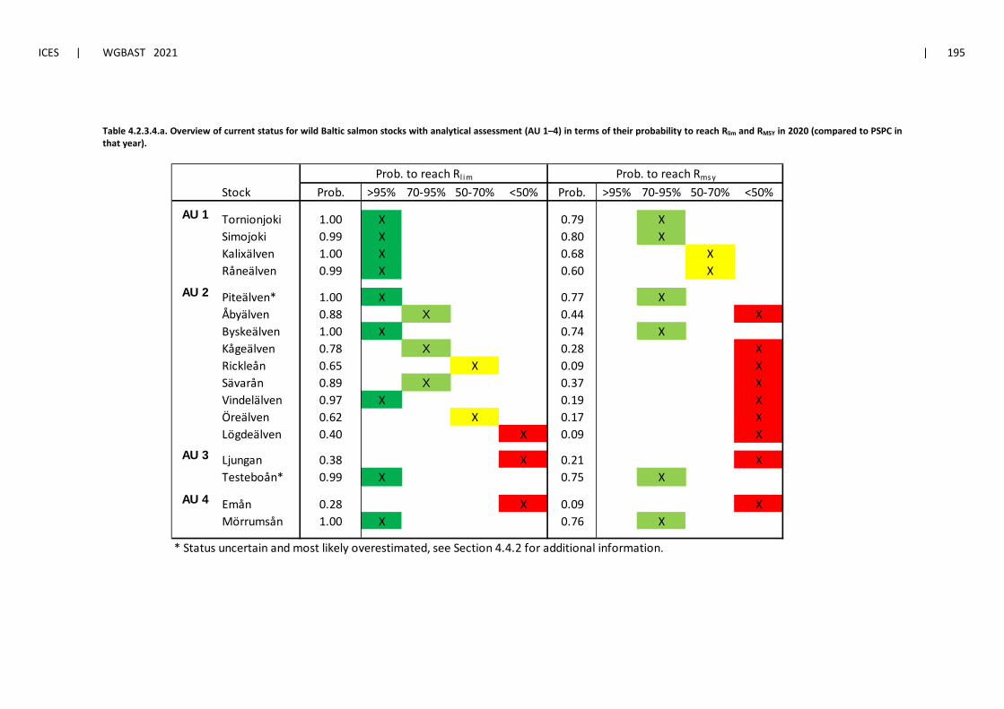
ICES | WGBAST 2021 | 195
Table 4.2.3.4.a. Overview of current status for wild Baltic salmon stocks with analytical assessment (AU 1–4) in terms of their probability to reach Rlim and RMSY in 2020 (compared to PSPC in that year).
Stock Prob. >95% 70-95% 50-70% <50% Prob. >95% 70-95% 50-70% <50%
Tornionjoki 1.00 X 0.79 XSimojoki 0.99 X 0.80 XKalixälven 1.00 X 0.68 XRåneälven 0.99 X 0.60 X
Piteälven* 1.00 X 0.77 XÅbyälven 0.88 X 0.44 XByskeälven 1.00 X 0.74 XKågeälven 0.78 X 0.28 XRickleån 0.65 X 0.09 XSävarån 0.89 X 0.37 XVindelälven 0.97 X 0.19 XÖreälven 0.62 X 0.17 XLögdeälven 0.40 X 0.09 X
Ljungan 0.38 X 0.21 XTesteboån* 0.99 X 0.75 X
Emån 0.28 X 0.09 XMörrumsån 1.00 X 0.76 X
* Status uncertain and most likely overestimated, see Section 4.4.2 for additional information.
AU 2
AU 3
AU 4
Prob. to reach Rl im Prob. to reach Rmsy
AU 1
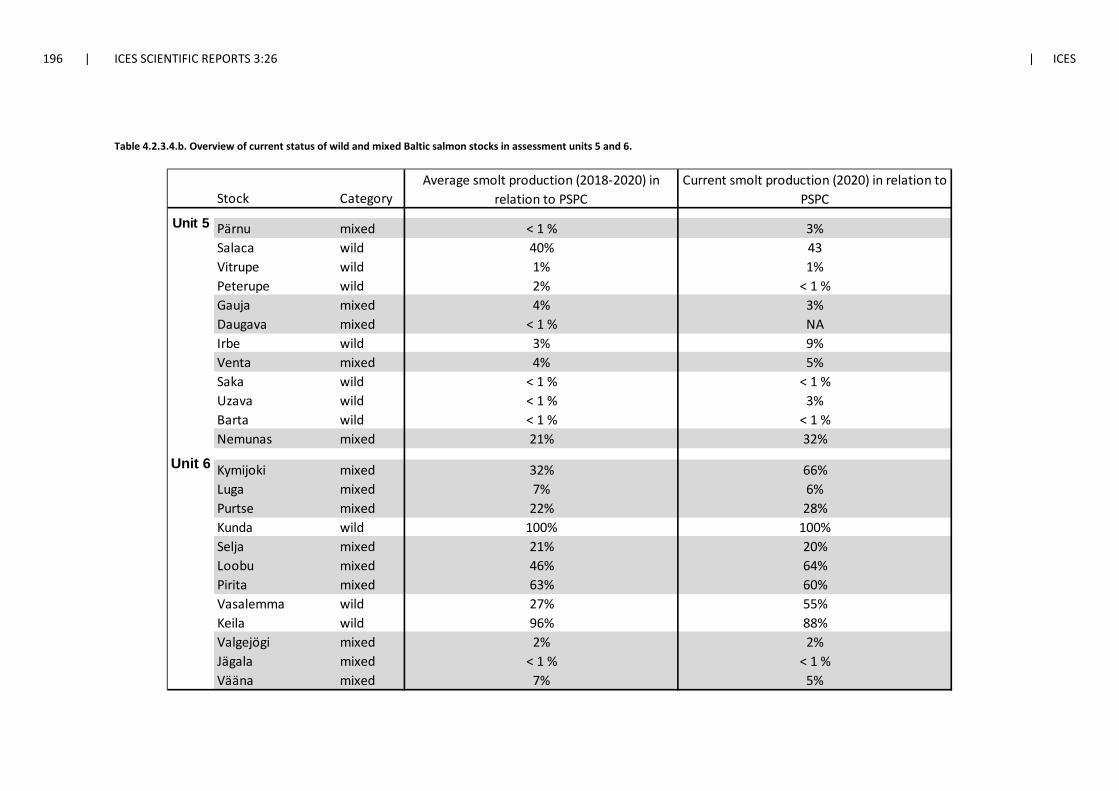
196 | ICES SCIENTIFIC REPORTS 3:26 | ICES
Table 4.2.3.4.b. Overview of current status of wild and mixed Baltic salmon stocks in assessment units 5 and 6.
Stock Category
Pärnu mixed < 1 % 3%Salaca wild 40% 43Vitrupe wild 1% 1%Peterupe wild 2% < 1 %Gauja mixed 4% 3%Daugava mixed < 1 % NAIrbe wild 3% 9%Venta mixed 4% 5%Saka wild < 1 % < 1 %Uzava wild < 1 % 3%Barta wild < 1 % < 1 %Nemunas mixed 21% 32%
Kymijoki mixed 32% 66%Luga mixed 7% 6%Purtse mixed 22% 28%Kunda wild 100% 100%Selja mixed 21% 20%Loobu mixed 46% 64%Pirita mixed 63% 60%Vasalemma wild 27% 55%Keila wild 96% 88%Valgejögi mixed 2% 2%Jägala mixed < 1 % < 1 %Vääna mixed 7% 5%
Unit 6
Unit 5
Average smolt production (2018-2020) in relation to PSPC
Current smolt production (2020) in relation to PSPC
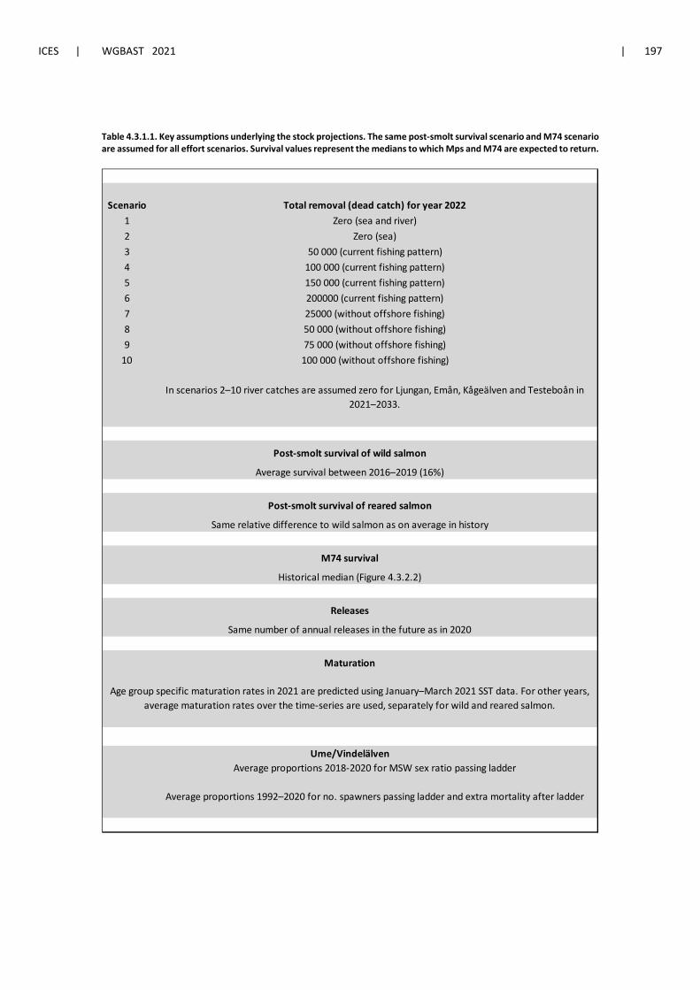
ICES | WGBAST 2021 | 197
Table 4.3.1.1. Key assumptions underlying the stock projections. The same post-smolt survival scenario and M74 scenario are assumed for all effort scenarios. Survival values represent the medians to which Mps and M74 are expected to return.
Scenario Total removal (dead catch) for year 20221 Zero (sea and river)2 Zero (sea)3 50 000 (current fishing pattern)4 100 000 (current fishing pattern)5 150 000 (current fishing pattern)6 200000 (current fishing pattern)7 25000 (without offshore fishing)8 50 000 (without offshore fishing)9 75 000 (without offshore fishing)
10 100 000 (without offshore fishing)
In scenarios 2–10 river catches are assumed zero for Ljungan, Emån, Kågeälven and Testeboån in 2021–2033.
Average proportions 2018-2020 for MSW sex ratio passing ladder
Average proportions 1992–2020 for no. spawners passing ladder and extra mortality after ladder
Ume/Vindelälven
Maturation
M74 survival
Same number of annual releases in the future as in 2020
Releases
Age group specific maturation rates in 2021 are predicted using January–March 2021 SST data. For other years, average maturation rates over the time-series are used, separately for wild and reared salmon.
Post-smolt survival of wild salmon
Average survival between 2016–2019 (16%)
Post-smolt survival of reared salmon
Same relative difference to wild salmon as on average in history
Historical median (Figure 4.3.2.2)
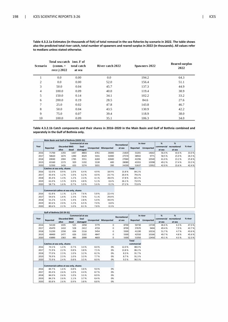
198 | ICES SCIENTIFIC REPORTS 3:26 | ICES
Table 4.3.2.1a Estimates (in thousands of fish) of total removal in the sea fisheries by scenario in 2022. The table shows also the predicted total river catch, total number of spawners and reared surplus in 2022 (in thousands). All values refer to medians unless stated otherwise.
Table 4.3.2.1b Catch components and their shares in 2016–2020 in the Main Basin and Gulf of Bothnia combined and separately in the Gulf of Bothnia only.
ScenarioTotal sea catch
(comm. + recr.) 2022
inst. F of total catch
at seaRiver catch 2022 Spawners 2022 Reared surplus
2022
1 0.0 0.00 0.0 194.2 64.32 0.0 0.00 52.0 156.4 51.13 50.0 0.04 45.7 137.3 44.94 100.0 0.09 40.0 119.4 38.95 150.0 0.14 34.1 102.2 33.26 200.0 0.19 28.5 84.6 27.67 25.0 0.02 47.8 143.8 46.78 50.0 0.04 43.5 130.9 42.29 75.0 0.07 39.4 118.9 38.010 100.0 0.09 35.1 106.3 34.0
Main Basin and Gulf of Bothnia (SD22-31)
alive dead2016 71700 1293 1447 8803 6761 26000 21820 53201 14642 56.4 % 10.6 % 33.0 %2017 58620 1674 1390 8329 5431 32000 27570 38942 9771 58.5 % 15.0 % 26.5 %2018 69040 1904 1785 3551 6269 42600 27060 42296 10540 61.0 % 13.2 % 25.8 %2019 65560 1573 929 5192 5530 600 28080 43355 10398 49.2 % 17.4 % 33.3 %2020 52350 1426 633 5274 5031 200 24200 52637 12952 42.0 % 15.6 % 42.4 %
Catches at sea only, shares Total 2016 52.0 % 0.9 % 1.0 % 6.4 % 4.9 % 18.9 % 15.8 % 84.2 %2017 43.4 % 1.2 % 1.0 % 6.2 % 4.0 % 23.7 % 20.4 % 79.6 %2018 45.4 % 1.3 % 1.2 % 2.3 % 4.1 % 28.0 % 17.8 % 82.2 %2019 61.0 % 1.5 % 0.9 % 4.8 % 5.1 % 0.6 % 26.1 % 73.9 %2020 58.7 % 1.6 % 0.7 % 5.9 % 5.6 % 0.2 % 27.2 % 72.8 %
Commercial cathes at sea only, shares2016 61.8 % 1.1 % 1.2 % 7.6 % 5.8 % 22.4 %2017 54.6 % 1.6 % 1.3 % 7.8 % 5.1 % 29.8 %2018 55.2 % 1.5 % 1.4 % 2.8 % 5.0 % 34.0 %2019 82.6 % 2.0 % 1.2 % 6.5 % 7.0 % 0.8 %2020 80.6 % 2.2 % 1.0 % 8.1 % 7.8 % 0.3 %
Gulf of Bothnia (SD 29-31)
alive dead2016 54130 1035 525 2458 5779 0 8700 50730 13728 46.6 % 6.3 % 47.0 %2017 45470 1410 528 2412 4724 0 8700 37670 9404 49.4 % 7.9 % 42.7 %2018 51230 1558 634 2116 5454 0 5500 41190 10216 51.7 % 4.7 % 43.6 %2019 48400 1477 626 2102 4847 0 5500 42550 10166 49.7 % 4.8 % 45.6 %2020 43890 1363 485 2008 4603 0 5500 51050 12450 43.1 % 4.5 % 52.3 %
Catches at sea only, sharesTotal commercial
2016 74.5 % 1.4 % 0.7 % 3.4 % 8.0 % 0% 12.0 % 88.0 %2017 71.9 % 2.2 % 0.8 % 3.8 % 7.5 % 0% 13.8 % 86.2 %2018 77.0 % 2.3 % 1.0 % 3.2 % 8.2 % 0% 8.3 % 91.7 %2019 76.9 % 2.3 % 1.0 % 3.3 % 7.7 % 0% 8.7 % 91.3 %2020 75.9 % 2.4 % 0.8 % 3.5 % 8.0 % 0% 9.5 % 90.5 %
Commercial cathes at sea only, shares2016 84.7 % 1.6 % 0.8 % 3.8 % 9.0 % 0%2017 83.4 % 2.6 % 1.0 % 4.4 % 8.7 % 0%2018 84.0 % 2.6 % 1.0 % 3.5 % 8.9 % 0%2019 84.2 % 2.6 % 1.1 % 3.7 % 8.4 % 0%2020 83.8 % 2.6 % 0.9 % 3.8 % 8.8 % 0%
YearIn river %
commercial at sea
% recreational
at seaReported Discarded BMS Seal
damagedUnreported Misreported Reported Unreported
Commercial at sea Recreational at sea
% river
Year%
commercial at sea
% recreational
at sea% river
In riverCommercial at sea Recreational at seaDiscarded BMSReported Seal
damagedUnreported Misreported Reported Unreported
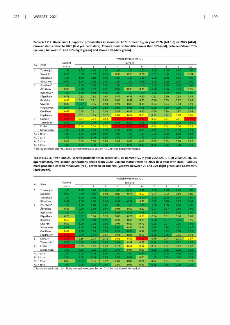
ICES | WGBAST 2021 | 199
Table 4.3.2.2. River- and AU-specific probabilities in scenarios 1-10 to meet Rlim in year 2026 (AU 1-3) or 2025 (AU4). Current status refers to 2020 (last year with data). Colours mark probabilities lower than 50% (red), between 50 and 70% (yellow), between 70 and 95% (light green) and above 95% (dark green).
Table 4.3.2.3. River- and AU-specific probabilities in scenarios 1-10 to meet Rlim in year 2055 (AU 1-3) or 2050 (AU 4), i.e. approximately five salmon generations ahead from 2020. Current status refers to 2020 (last year with data). Colours mark probabilities lower than 50% (red), between 50 and 70% (yellow), between 70 and 95% (light green) and above 95% (dark green).
Probability to meet Rl im
Scenario1 2 3 4 5 6 7 8 9 10
1 Tornionjoki 1.00 1.00 1.00 1.00 1.00 1.00 1.00 1.00 1.00 1.00 1.00Simojoki 0.99 0.99 0.97 0.97 0.95 0.93 0.88 0.97 0.96 0.95 0.94Kalixälven 1.00 1.00 1.00 1.00 1.00 1.00 1.00 1.00 1.00 1.00 1.00Råneälven 0.99 1.00 1.00 1.00 1.00 1.00 0.99 1.00 1.00 1.00 1.00
2 Piteälven* 1.00 1.00 1.00 1.00 1.00 1.00 1.00 1.00 1.00 1.00 1.00Åbyälven 0.88 0.98 0.97 0.96 0.95 0.93 0.91 0.96 0.96 0.95 0.95Byskeälven 1.00 1.00 1.00 1.00 1.00 1.00 1.00 1.00 1.00 1.00 1.00Kågeälven 0.78 0.92 0.92 0.90 0.87 0.83 0.80 0.91 0.90 0.88 0.86Rickleån 0.65 0.95 0.91 0.89 0.86 0.81 0.75 0.90 0.89 0.87 0.84Sävarån 0.89 0.97 0.95 0.94 0.92 0.89 0.85 0.94 0.94 0.93 0.91Vindelälven 0.97 1.00 0.99 0.99 0.99 0.98 0.96 0.99 0.99 0.99 0.98Öreälven 0.62 0.95 0.91 0.89 0.87 0.84 0.80 0.90 0.89 0.87 0.86Lögdeälven 0.40 0.81 0.75 0.72 0.67 0.62 0.55 0.73 0.72 0.69 0.66
3 Ljungan 0.38 0.54 0.54 0.52 0.49 0.46 0.42 0.53 0.51 0.51 0.49Testeboån* 0.99 0.99 0.99 0.98 0.98 0.97 0.96 0.99 0.98 0.98 0.98
4 Emån 0.28 0.54 0.54 0.51 0.49 0.46 0.43 0.54 0.54 0.54 0.54Mörrumsån 1.00 1.00 0.99 0.99 0.99 0.99 0.98 0.99 0.99 0.99 0.99
AU 1 total 1.00 1.00 1.00 1.00 1.00 1.00 1.00 1.00 1.00 1.00 1.00AU 2 total 1.00 1.00 1.00 1.00 1.00 1.00 1.00 1.00 1.00 1.00 1.00AU 3 total 0.86 0.89 0.89 0.89 0.87 0.85 0.83 0.89 0.89 0.88 0.87AU 4 total 1.00 0.99 0.98 0.98 0.98 0.97 0.97 0.98 0.98 0.98 0.98* Status uncertain and most likely overestimated, see Section 4.4.2 for additional information.
RiverCurrent status
AU
Probability to meet Rl im
Scenario1 2 3 4 5 6 7 8 9 10
1 Tornionjoki 1.00 1.00 1.00 1.00 1.00 0.99 0.98 1.00 1.00 1.00 1.00Simojoki 0.99 0.99 0.96 0.91 0.85 0.75 0.57 0.94 0.92 0.89 0.85Kalixälven 1.00 1.00 1.00 1.00 1.00 1.00 1.00 1.00 1.00 1.00 1.00Råneälven 0.99 1.00 1.00 0.99 0.99 0.98 0.95 0.99 0.99 0.99 0.99
2 Piteälven* 1.00 1.00 1.00 1.00 1.00 1.00 1.00 1.00 1.00 1.00 1.00Åbyälven 0.88 0.99 0.98 0.97 0.94 0.90 0.82 0.97 0.97 0.96 0.96Byskeälven 1.00 1.00 1.00 1.00 0.99 0.99 0.98 1.00 1.00 1.00 1.00Kågeälven 0.78 0.97 0.94 0.91 0.86 0.79 0.69 0.94 0.91 0.90 0.88Rickleån 0.65 0.99 0.98 0.96 0.93 0.88 0.79 0.98 0.97 0.96 0.95Sävarån 0.89 1.00 0.98 0.96 0.94 0.89 0.77 0.98 0.97 0.96 0.95Vindelälven 0.97 1.00 0.99 0.98 0.96 0.93 0.86 0.98 0.98 0.97 0.97Öreälven 0.62 1.00 0.99 0.99 0.98 0.96 0.92 0.99 0.99 0.98 0.98Lögdeälven 0.40 0.99 0.97 0.95 0.91 0.84 0.72 0.96 0.96 0.95 0.93
3 Ljungan 0.38 0.86 0.78 0.71 0.62 0.52 0.41 0.76 0.74 0.71 0.67Testeboån* 0.99 0.99 0.98 0.97 0.95 0.92 0.87 0.98 0.98 0.97 0.96
4 Emån 0.28 0.89 0.82 0.78 0.72 0.64 0.54 0.82 0.82 0.82 0.82Mörrumsån 1.00 0.99 0.98 0.97 0.96 0.95 0.92 0.98 0.98 0.98 0.98
AU 1 total 1.00 1.00 1.00 1.00 1.00 1.00 0.99 1.00 1.00 1.00 1.00AU 2 total 1.00 1.00 1.00 0.99 0.99 0.97 0.95 1.00 0.99 0.99 0.99AU 3 total 0.86 0.97 0.94 0.92 0.88 0.82 0.74 0.94 0.93 0.91 0.90AU 4 total 1.00 0.99 0.98 0.96 0.95 0.93 0.91 0.98 0.98 0.98 0.98* Status uncertain and most likely overestimated, see Section 4.4.2 for additional information.
RiverCurrent status
AU
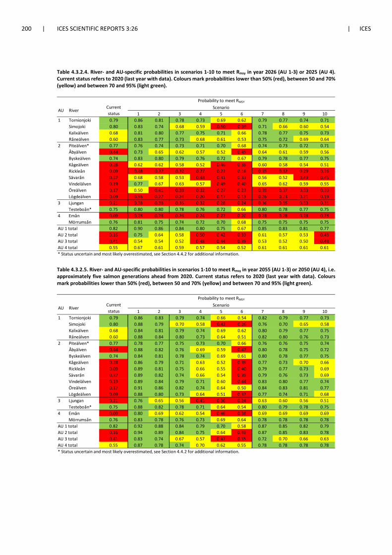
200 | ICES SCIENTIFIC REPORTS 3:26 | ICES
Table 4.3.2.4. River- and AU-specific probabilities in scenarios 1-10 to meet Rmsy in year 2026 (AU 1-3) or 2025 (AU 4). Current status refers to 2020 (last year with data). Colours mark probabilities lower than 50% (red), between 50 and 70% (yellow) and between 70 and 95% (light green).
Table 4.3.2.5. River- and AU-specific probabilities in scenarios 1-10 to meet Rmsy in year 2055 (AU 1-3) or 2050 (AU 4), i.e. approximately five salmon generations ahead from 2020. Current status refers to 2020 (last year with data). Colours mark probabilities lower than 50% (red), between 50 and 70% (yellow) and between 70 and 95% (light green).
Probability to meet RMSY
Scenario1 2 3 4 5 6 7 8 9 10
1 Tornionjoki 0.79 0.86 0.81 0.78 0.73 0.69 0.62 0.79 0.77 0.74 0.71Simojoki 0.80 0.83 0.74 0.68 0.59 0.50 0.39 0.71 0.66 0.60 0.54Kalixälven 0.68 0.81 0.80 0.77 0.75 0.71 0.66 0.78 0.77 0.75 0.73Råneälven 0.60 0.83 0.77 0.73 0.68 0.61 0.53 0.75 0.72 0.69 0.64
2 Piteälven* 0.77 0.76 0.74 0.73 0.71 0.70 0.68 0.74 0.73 0.72 0.71Åbyälven 0.44 0.73 0.65 0.62 0.57 0.52 0.45 0.64 0.61 0.59 0.56Byskeälven 0.74 0.83 0.80 0.79 0.76 0.72 0.67 0.79 0.78 0.77 0.75Kågeälven 0.28 0.62 0.62 0.58 0.52 0.46 0.38 0.60 0.58 0.54 0.51Rickleån 0.09 0.48 0.37 0.32 0.27 0.22 0.16 0.35 0.32 0.29 0.26Sävarån 0.37 0.68 0.58 0.53 0.48 0.41 0.33 0.56 0.52 0.49 0.45Vindelälven 0.19 0.77 0.67 0.63 0.57 0.49 0.40 0.65 0.62 0.59 0.55Öreälven 0.17 0.50 0.41 0.38 0.32 0.27 0.23 0.39 0.37 0.33 0.30Lögdeälven 0.09 0.36 0.27 0.24 0.20 0.17 0.13 0.26 0.23 0.21 0.19
3 Ljungan 0.21 0.38 0.38 0.35 0.32 0.28 0.24 0.36 0.35 0.33 0.31Testeboån* 0.75 0.80 0.80 0.78 0.76 0.72 0.66 0.80 0.78 0.77 0.75
4 Emån 0.09 0.28 0.28 0.26 0.24 0.22 0.20 0.28 0.28 0.28 0.28Mörrumsån 0.76 0.81 0.75 0.74 0.72 0.70 0.68 0.75 0.75 0.75 0.75
AU 1 total 0.82 0.90 0.86 0.84 0.80 0.75 0.67 0.85 0.83 0.81 0.77AU 2 total 0.16 0.75 0.64 0.58 0.50 0.42 0.33 0.61 0.57 0.53 0.48AU 3 total 0.41 0.54 0.54 0.52 0.48 0.44 0.39 0.53 0.52 0.50 0.48AU 4 total 0.55 0.67 0.61 0.59 0.57 0.54 0.52 0.61 0.61 0.61 0.61* Status uncertain and most likely overestimated, see Section 4.4.2 for additional information.
RiverCurrent status
AU
Probability to meet RMSY
Scenario1 2 3 4 5 6 7 8 9 10
1 Tornionjoki 0.79 0.86 0.83 0.79 0.74 0.66 0.54 0.82 0.79 0.77 0.73Simojoki 0.80 0.88 0.79 0.70 0.58 0.42 0.26 0.76 0.70 0.65 0.58Kalixälven 0.68 0.84 0.81 0.79 0.74 0.69 0.62 0.80 0.79 0.77 0.75Råneälven 0.60 0.88 0.84 0.80 0.73 0.64 0.51 0.82 0.80 0.76 0.73
2 Piteälven* 0.77 0.78 0.77 0.75 0.73 0.70 0.66 0.76 0.76 0.75 0.74Åbyälven 0.44 0.88 0.82 0.76 0.69 0.59 0.47 0.80 0.78 0.75 0.72Byskeälven 0.74 0.84 0.81 0.78 0.74 0.69 0.61 0.80 0.78 0.77 0.75Kågeälven 0.28 0.86 0.79 0.71 0.63 0.52 0.39 0.77 0.73 0.70 0.66Rickleån 0.09 0.89 0.81 0.75 0.66 0.55 0.40 0.79 0.77 0.73 0.69Sävarån 0.37 0.89 0.82 0.74 0.66 0.54 0.39 0.79 0.76 0.73 0.69Vindelälven 0.19 0.89 0.84 0.79 0.71 0.60 0.44 0.83 0.80 0.77 0.74Öreälven 0.17 0.91 0.86 0.82 0.74 0.64 0.50 0.84 0.83 0.81 0.77Lögdeälven 0.09 0.88 0.80 0.73 0.64 0.51 0.37 0.77 0.74 0.71 0.68
3 Ljungan 0.21 0.76 0.65 0.56 0.45 0.36 0.24 0.63 0.60 0.56 0.51Testeboån* 0.75 0.88 0.82 0.78 0.71 0.64 0.54 0.80 0.79 0.78 0.75
4 Emån 0.09 0.80 0.69 0.62 0.54 0.46 0.38 0.69 0.69 0.69 0.69Mörrumsån 0.76 0.83 0.78 0.76 0.73 0.69 0.64 0.78 0.78 0.78 0.78
AU 1 total 0.82 0.92 0.88 0.84 0.79 0.70 0.58 0.87 0.85 0.82 0.79AU 2 total 0.16 0.94 0.89 0.84 0.75 0.64 0.49 0.87 0.85 0.83 0.78AU 3 total 0.41 0.83 0.74 0.67 0.57 0.47 0.35 0.72 0.70 0.66 0.63AU 4 total 0.55 0.87 0.78 0.74 0.70 0.62 0.55 0.78 0.78 0.78 0.78* Status uncertain and most likely overestimated, see Section 4.4.2 for additional information.
RiverCurrent status
AU
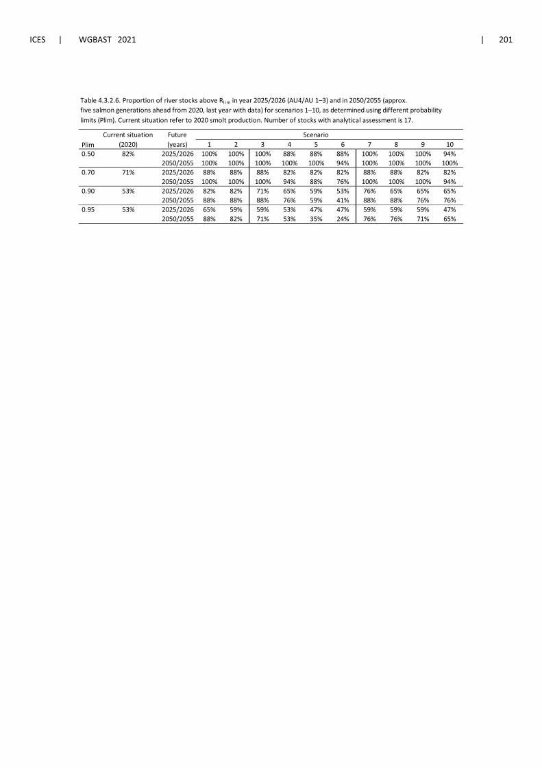
ICES | WGBAST 2021 | 201
Table 4.3.2.6. Proportion of river stocks above Rl im in year 2025/2026 (AU4/AU 1–3) and in 2050/2055 (approx.five salmon generations ahead from 2020, last year with data) for scenarios 1–10, as determined using different probabilitylimits (Plim). Current situation refer to 2020 smolt production. Number of stocks with analytical assessment is 17.
ScenarioPlim 1 2 3 4 5 6 7 8 9 100.50 82% 2025/2026 100% 100% 100% 88% 88% 88% 100% 100% 100% 94%
2050/2055 100% 100% 100% 100% 100% 94% 100% 100% 100% 100%0.70 71% 2025/2026 88% 88% 88% 82% 82% 82% 88% 88% 82% 82%
2050/2055 100% 100% 100% 94% 88% 76% 100% 100% 100% 94%0.90 53% 2025/2026 82% 82% 71% 65% 59% 53% 76% 65% 65% 65%
2050/2055 88% 88% 88% 76% 59% 41% 88% 88% 76% 76%0.95 53% 2025/2026 65% 59% 59% 53% 47% 47% 59% 59% 59% 47%
2050/2055 88% 82% 71% 53% 35% 24% 76% 76% 71% 65%
Current situation (2020)
Future (years)
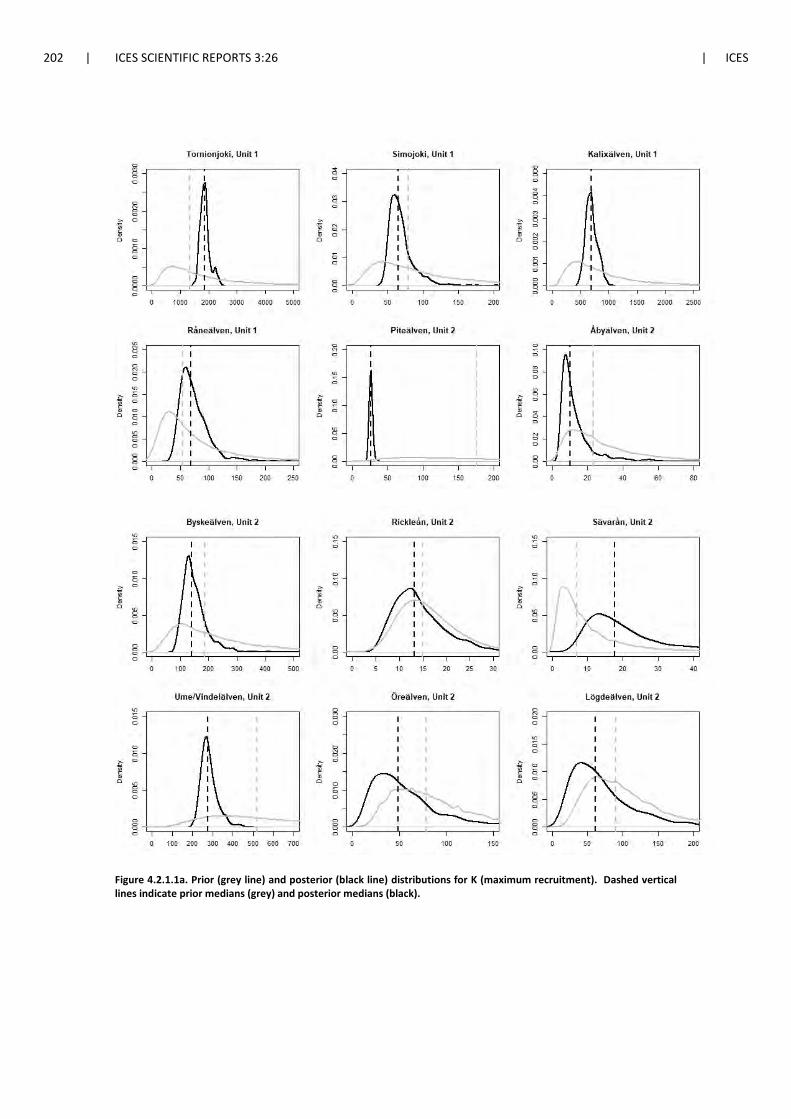
202 | ICES SCIENTIFIC REPORTS 3:26 | ICES
Figure 4.2.1.1a. Prior (grey line) and posterior (black line) distributions for K (maximum recruitment). Dashed vertical lines indicate prior medians (grey) and posterior medians (black).
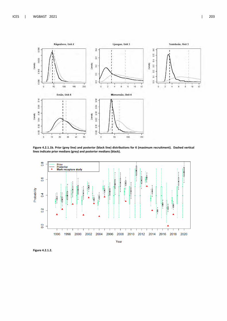
ICES | WGBAST 2021 | 203
Figure 4.2.1.1b. Prior (grey line) and posterior (black line) distributions for K (maximum recruitment). Dashed vertical lines indicate prior medians (grey) and posterior medians (black).
Figure 4.2.1.2.
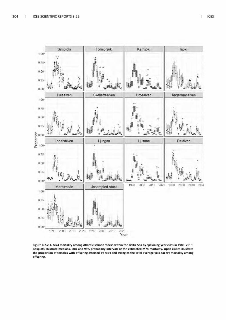
204 | ICES SCIENTIFIC REPORTS 3:26 | ICES
Figure 4.2.2.1. M74 mortality among Atlantic salmon stocks within the Baltic Sea by spawning year class in 1985–2019. Boxplots illustrate medians, 50% and 95% probability intervals of the estimated M74 mortality. Open circles illustrate the proportion of females with offspring affected by M74 and triangles the total average yolk-sac-fry mortality among offspring.
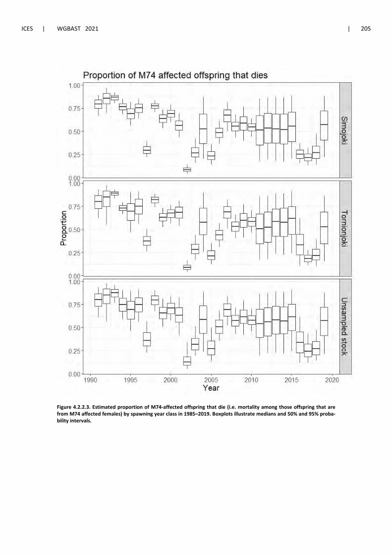
ICES | WGBAST 2021 | 205
Figure 4.2.2.3. Estimated proportion of M74-affected offspring that die (i.e. mortality among those offspring that are from M74 affected females) by spawning year class in 1985–2019. Boxplots illustrate medians and 50% and 95% proba-bility intervals.
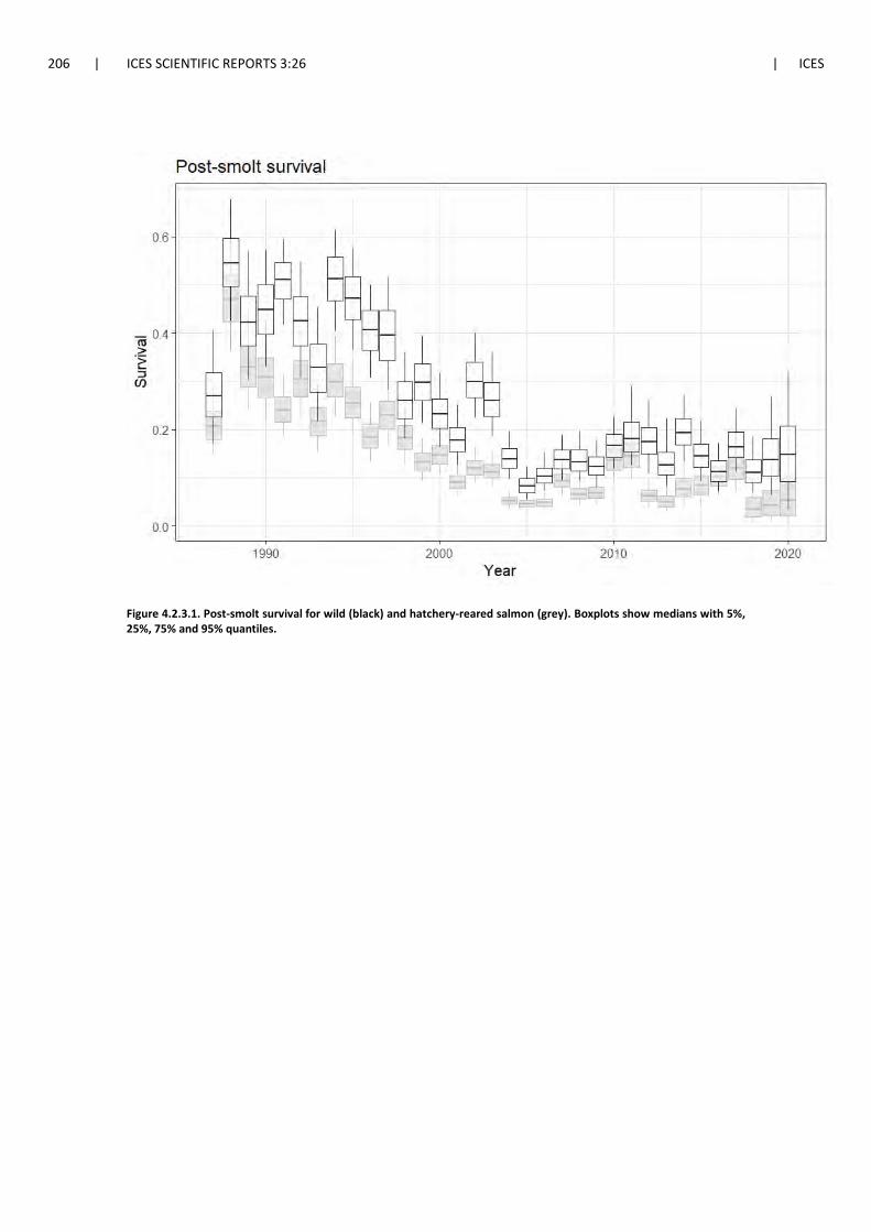
206 | ICES SCIENTIFIC REPORTS 3:26 | ICES
Figure 4.2.3.1. Post-smolt survival for wild (black) and hatchery-reared salmon (grey). Boxplots show medians with 5%, 25%, 75% and 95% quantiles.
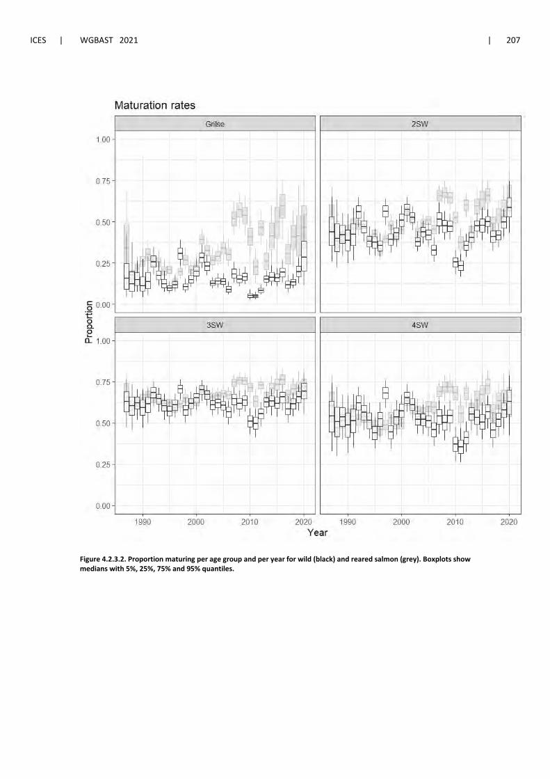
ICES | WGBAST 2021 | 207
Figure 4.2.3.2. Proportion maturing per age group and per year for wild (black) and reared salmon (grey). Boxplots show medians with 5%, 25%, 75% and 95% quantiles.
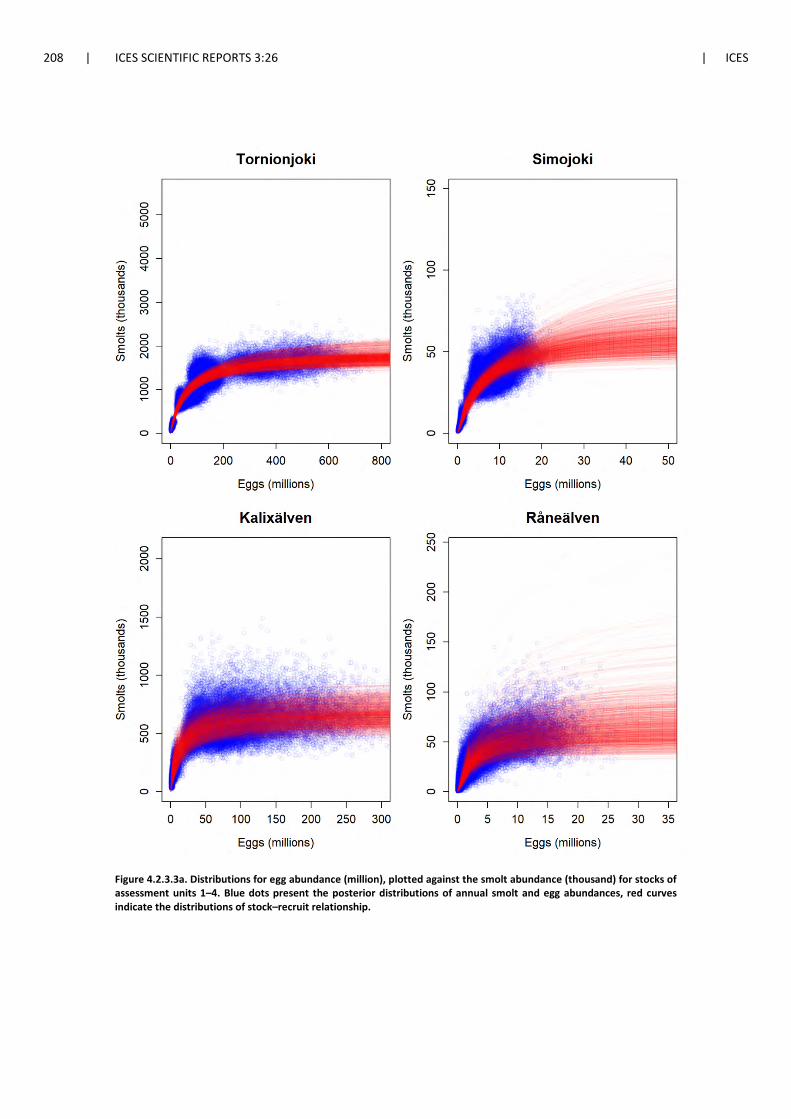
208 | ICES SCIENTIFIC REPORTS 3:26 | ICES
Figure 4.2.3.3a. Distributions for egg abundance (million), plotted against the smolt abundance (thousand) for stocks of assessment units 1–4. Blue dots present the posterior distributions of annual smolt and egg abundances, red curves indicate the distributions of stock–recruit relationship.
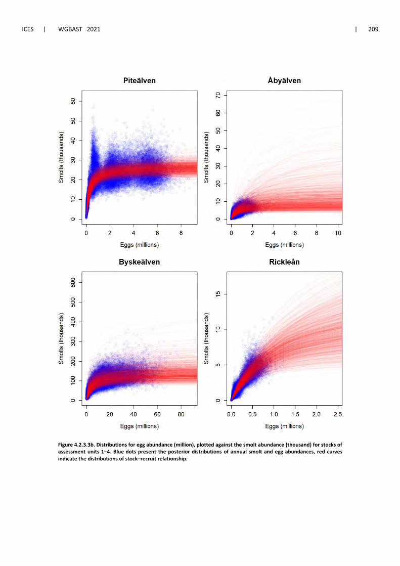
ICES | WGBAST 2021 | 209
Figure 4.2.3.3b. Distributions for egg abundance (million), plotted against the smolt abundance (thousand) for stocks of assessment units 1–4. Blue dots present the posterior distributions of annual smolt and egg abundances, red curves indicate the distributions of stock–recruit relationship.
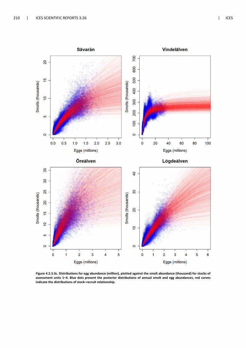
210 | ICES SCIENTIFIC REPORTS 3:26 | ICES
Figure 4.2.3.3c. Distributions for egg abundance (million), plotted against the smolt abundance (thousand) for stocks of assessment units 1–4. Blue dots present the posterior distributions of annual smolt and egg abundances, red curves indicate the distributions of stock–recruit relationship.
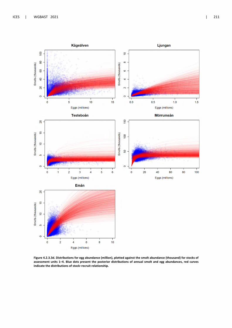
ICES | WGBAST 2021 | 211
Figure 4.2.3.3d. Distributions for egg abundance (million), plotted against the smolt abundance (thousand) for stocks of assessment units 1–4. Blue dots present the posterior distributions of annual smolt and egg abundances, red curves indicate the distributions of stock–recruit relationship.
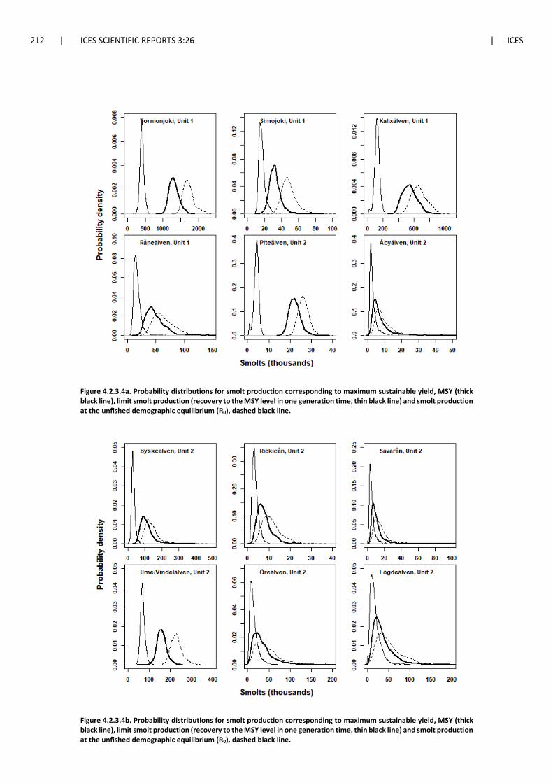
212 | ICES SCIENTIFIC REPORTS 3:26 | ICES
Figure 4.2.3.4a. Probability distributions for smolt production corresponding to maximum sustainable yield, MSY (thick black line), limit smolt production (recovery to the MSY level in one generation time, thin black line) and smolt production at the unfished demographic equilibrium (R0), dashed black line.
Figure 4.2.3.4b. Probability distributions for smolt production corresponding to maximum sustainable yield, MSY (thick black line), limit smolt production (recovery to the MSY level in one generation time, thin black line) and smolt production at the unfished demographic equilibrium (R0), dashed black line.
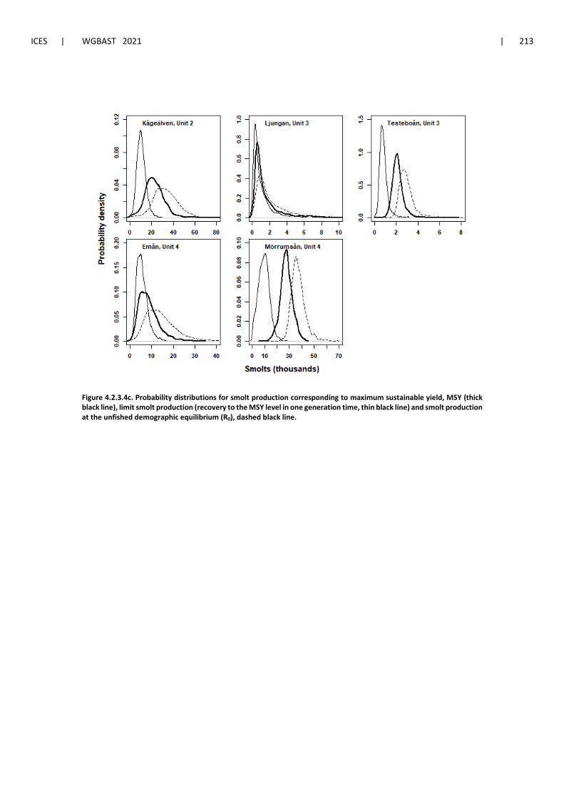
ICES | WGBAST 2021 | 213
Figure 4.2.3.4c. Probability distributions for smolt production corresponding to maximum sustainable yield, MSY (thick black line), limit smolt production (recovery to the MSY level in one generation time, thin black line) and smolt production at the unfished demographic equilibrium (R0), dashed black line.
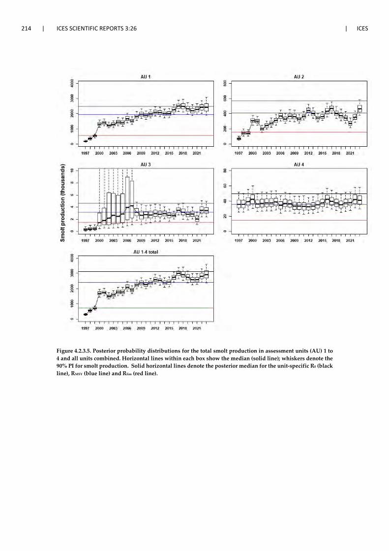
214 | ICES SCIENTIFIC REPORTS 3:26 | ICES
Figure 4.2.3.5. Posterior probability distributions for the total smolt production in assessment units (AU) 1 to 4 and all units combined. Horizontal lines within each box show the median (solid line); whiskers denote the 90% PI for smolt production. Solid horizontal lines denote the posterior median for the unit-specific R0 (black line), RMSY (blue line) and Rlim (red line).
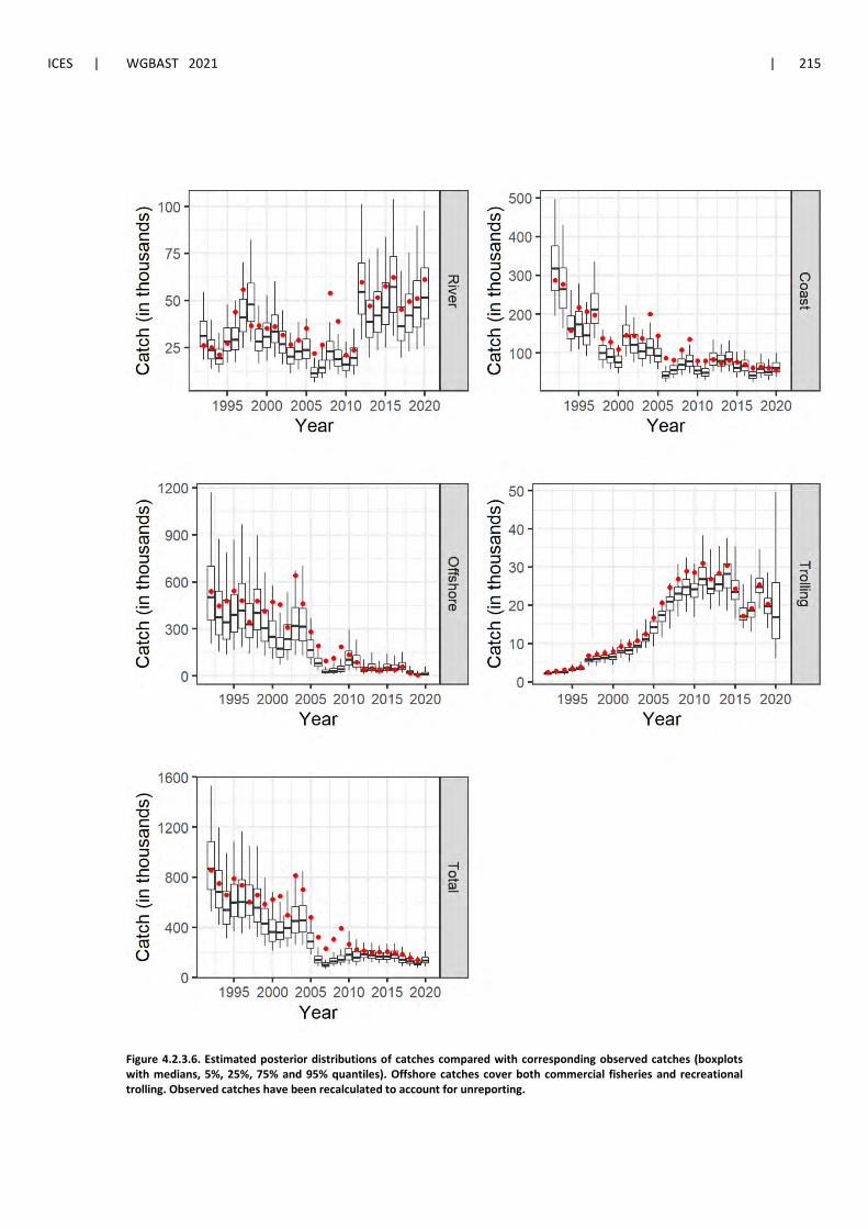
ICES | WGBAST 2021 | 215
Figure 4.2.3.6. Estimated posterior distributions of catches compared with corresponding observed catches (boxplots with medians, 5%, 25%, 75% and 95% quantiles). Offshore catches cover both commercial fisheries and recreational trolling. Observed catches have been recalculated to account for unreporting.
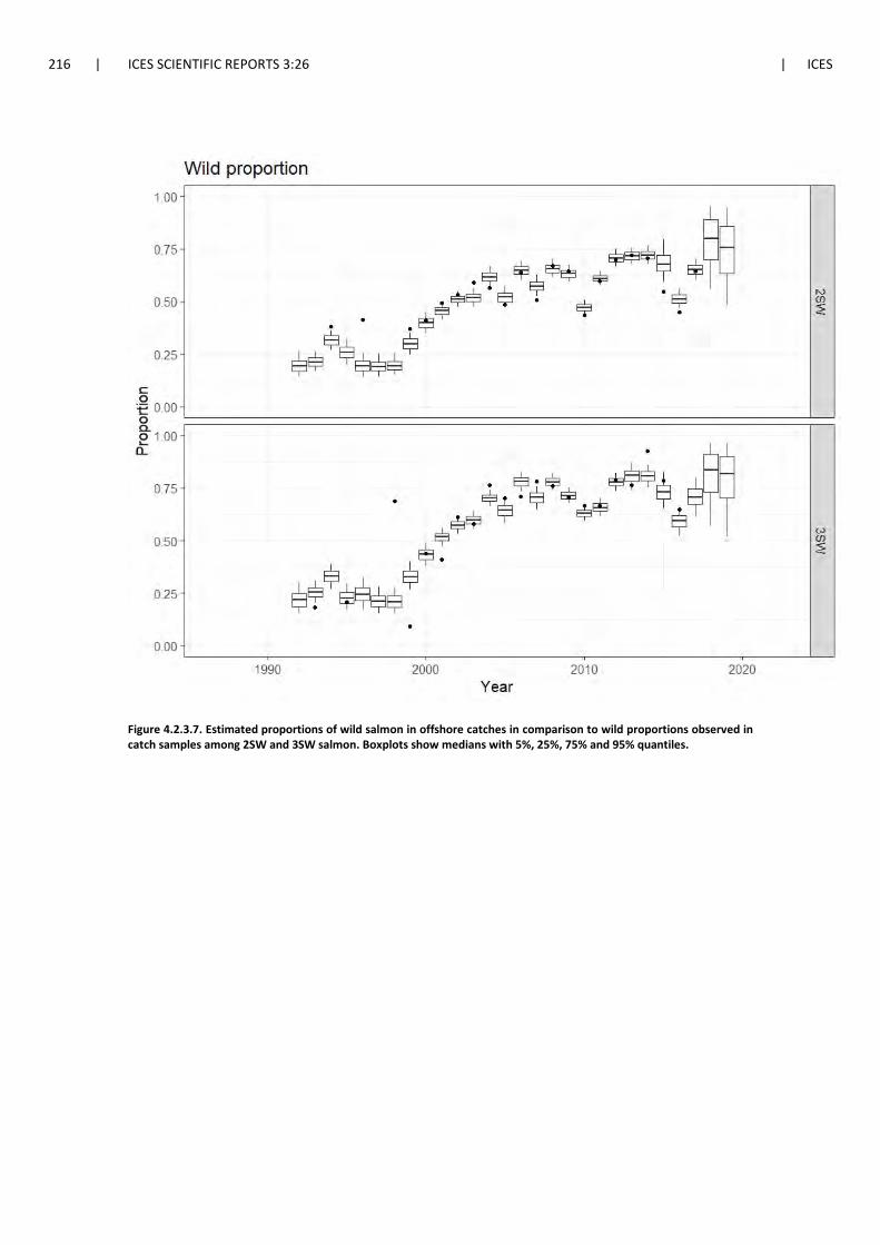
216 | ICES SCIENTIFIC REPORTS 3:26 | ICES
Figure 4.2.3.7. Estimated proportions of wild salmon in offshore catches in comparison to wild proportions observed in catch samples among 2SW and 3SW salmon. Boxplots show medians with 5%, 25%, 75% and 95% quantiles.
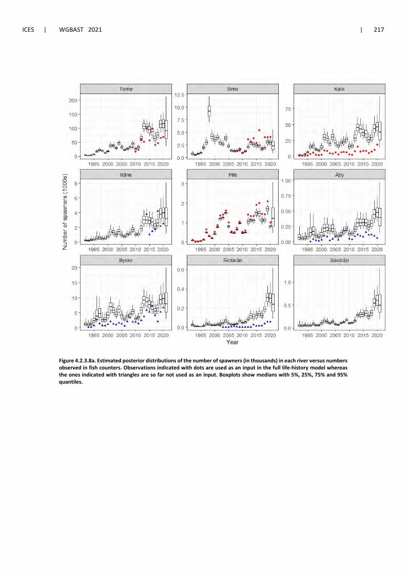
ICES | WGBAST 2021 | 217
Figure 4.2.3.8a. Estimated posterior distributions of the number of spawners (in thousands) in each river versus numbers observed in fish counters. Observations indicated with dots are used as an input in the full life-history model whereas the ones indicated with triangles are so far not used as an input. Boxplots show medians with 5%, 25%, 75% and 95% quantiles.
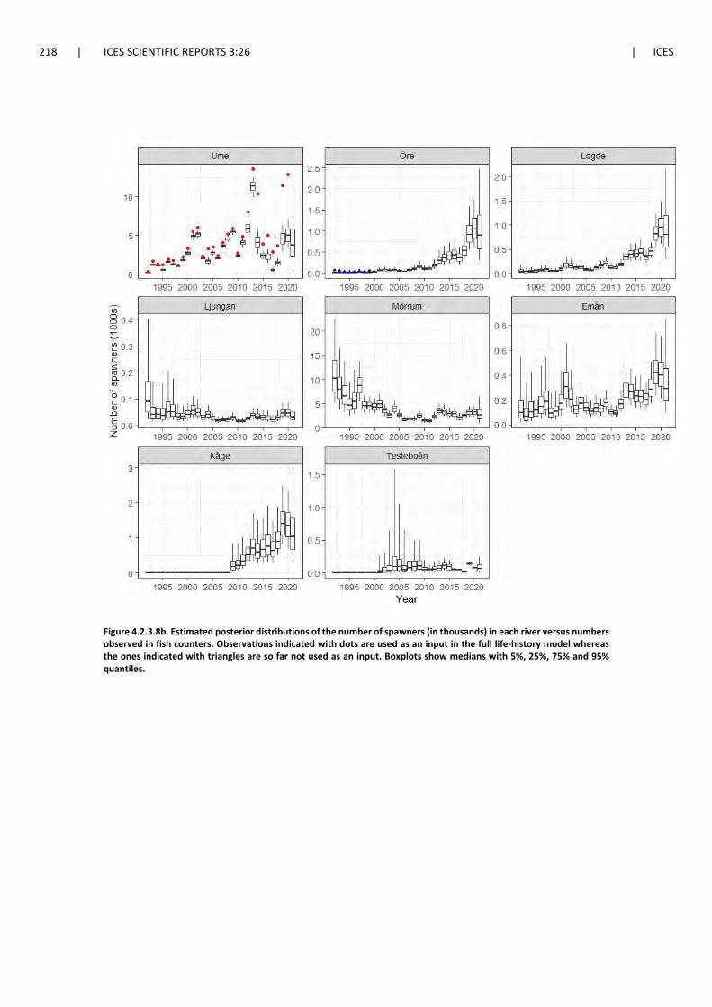
218 | ICES SCIENTIFIC REPORTS 3:26 | ICES
Figure 4.2.3.8b. Estimated posterior distributions of the number of spawners (in thousands) in each river versus numbers observed in fish counters. Observations indicated with dots are used as an input in the full life-history model whereas the ones indicated with triangles are so far not used as an input. Boxplots show medians with 5%, 25%, 75% and 95% quantiles.
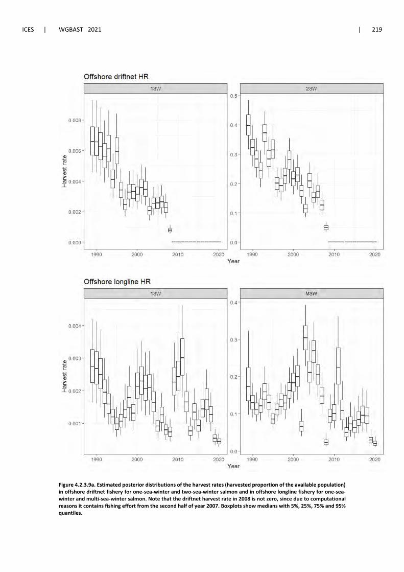
ICES | WGBAST 2021 | 219
Figure 4.2.3.9a. Estimated posterior distributions of the harvest rates (harvested proportion of the available population) in offshore driftnet fishery for one-sea-winter and two-sea-winter salmon and in offshore longline fishery for one-sea-winter and multi-sea-winter salmon. Note that the driftnet harvest rate in 2008 is not zero, since due to computational reasons it contains fishing effort from the second half of year 2007. Boxplots show medians with 5%, 25%, 75% and 95% quantiles.
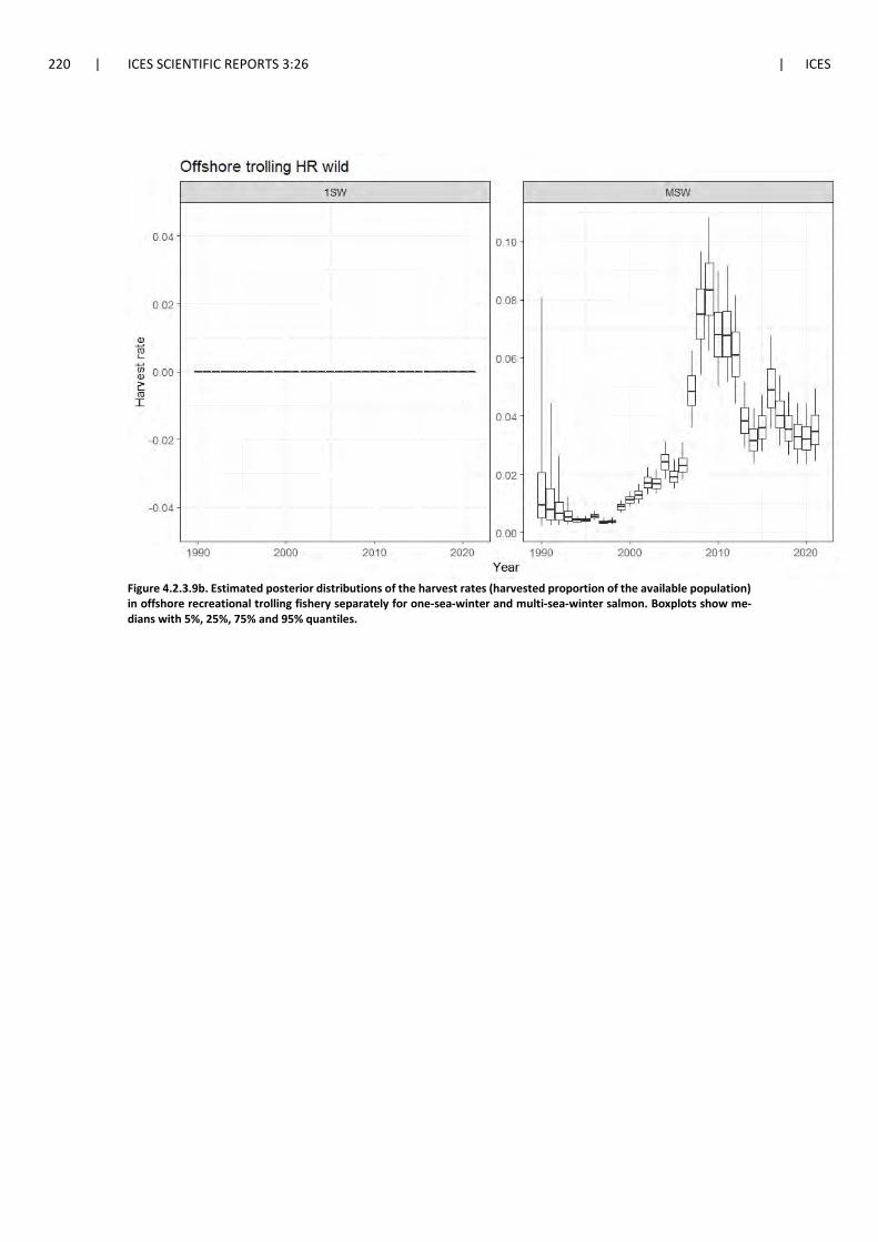
220 | ICES SCIENTIFIC REPORTS 3:26 | ICES
Figure 4.2.3.9b. Estimated posterior distributions of the harvest rates (harvested proportion of the available population) in offshore recreational trolling fishery separately for one-sea-winter and multi-sea-winter salmon. Boxplots show me-dians with 5%, 25%, 75% and 95% quantiles.
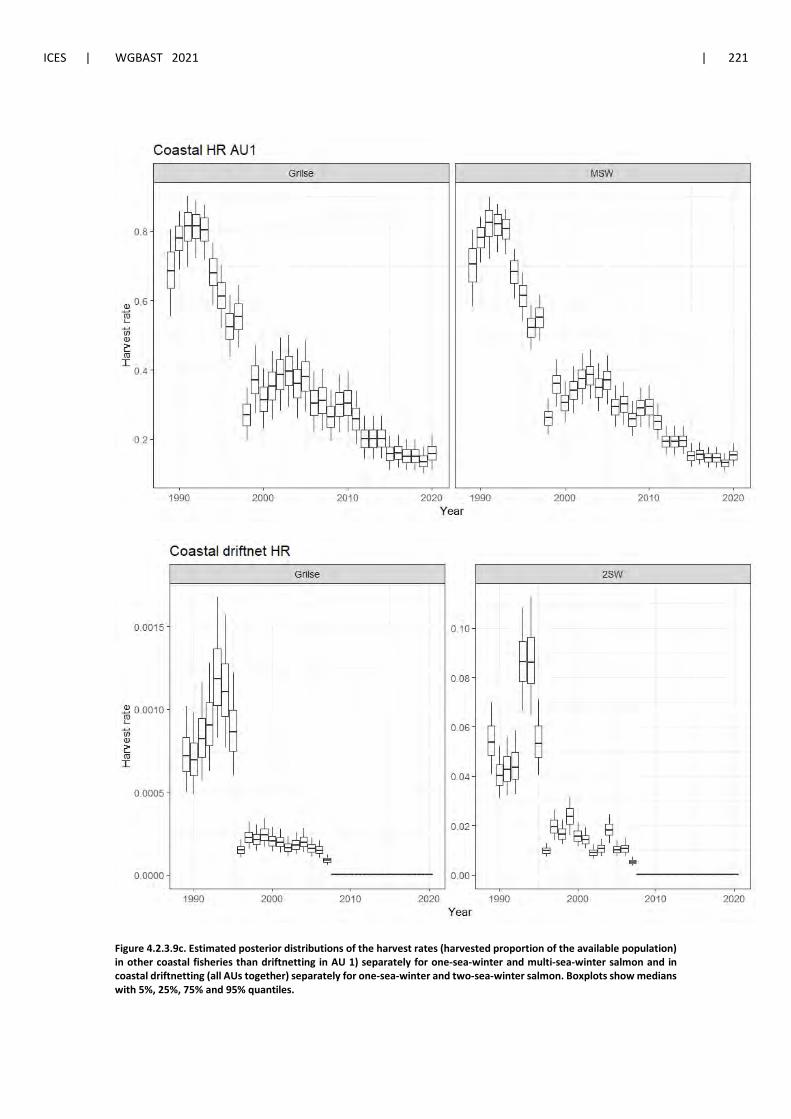
ICES | WGBAST 2021 | 221
Figure 4.2.3.9c. Estimated posterior distributions of the harvest rates (harvested proportion of the available population) in other coastal fisheries than driftnetting in AU 1) separately for one-sea-winter and multi-sea-winter salmon and in coastal driftnetting (all AUs together) separately for one-sea-winter and two-sea-winter salmon. Boxplots show medians with 5%, 25%, 75% and 95% quantiles.
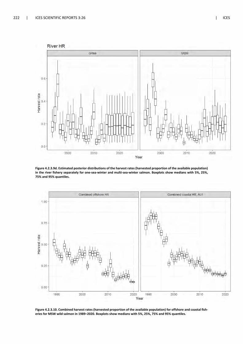
222 | ICES SCIENTIFIC REPORTS 3:26 | ICES
Figure 4.2.3.9d. Estimated posterior distributions of the harvest rates (harvested proportion of the available population) in the river fishery separately for one-sea-winter and multi-sea-winter salmon. Boxplots show medians with 5%, 25%, 75% and 95% quantiles.
Figure 4.2.3.10. Combined harvest rates (harvested proportion of the available population) for offshore and coastal fish-eries for MSW wild salmon in 1989–2020. Boxplots show medians with 5%, 25%, 75% and 95% quantiles.
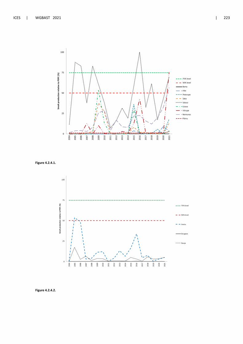
ICES | WGBAST 2021 | 223
Figure 4.2.4.1.
Figure 4.2.4.2.
0
25
50
75
100
2004
2005
2006
2007
2008
2009
2010
2011
2012
2013
2014
2015
2016
2017
2018
2019
2020
2021
Smol
t pro
duct
ion
rela
tive
to P
SPC
(%)
75% level
50% level
Barta
Irbe
Peterupe
Saka
Salaca
Uzava
Vitrupe
Nemunas
Pärnu
0
25
50
75
100
2004
2005
2006
2007
2008
2009
2010
2011
2012
2013
2014
2015
2016
2017
2018
2019
2020
2021
Smol
t pro
duct
ion
rela
tive
to P
SPC
(%)
75% level
50% level
Venta
Daugava
Gauja
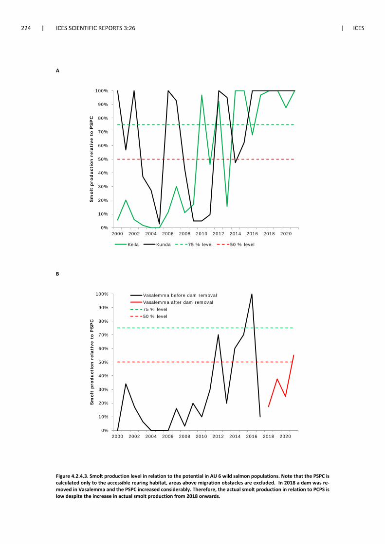
224 | ICES SCIENTIFIC REPORTS 3:26 | ICES
A
B
Figure 4.2.4.3. Smolt production level in relation to the potential in AU 6 wild salmon populations. Note that the PSPC is calculated only to the accessible rearing habitat, areas above migration obstacles are excluded. In 2018 a dam was re-moved in Vasalemma and the PSPC increased considerably. Therefore, the actual smolt production in relation to PCPS is low despite the increase in actual smolt production from 2018 onwards.
0%
10%
20%
30%
40%
50%
60%
70%
80%
90%
100%
2000 2002 2004 2006 2008 2010 2012 2014 2016 2018 2020
Sm
olt
pro
du
ctio
n r
elat
ive
to P
SP
C
Keila Kunda 75 % level 50 % level
0%
10%
20%
30%
40%
50%
60%
70%
80%
90%
100%
2000 2002 2004 2006 2008 2010 2012 2014 2016 2018 2020
Sm
olt
pro
du
ctio
n r
elat
ive
to P
SP
C
Vasalemma before dam removalVasalemma after dam removal75 % level50 % level
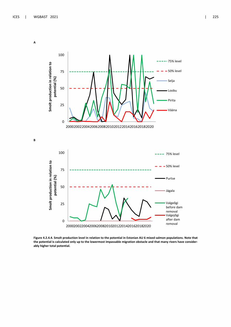
ICES | WGBAST 2021 | 225
A
B
Figure 4.2.4.4. Smolt production level in relation to the potential in Estonian AU 6 mixed salmon populations. Note that the potential is calculated only up to the lowermost impassable migration obstacle and that many rivers have consider-ably higher total potential.
0
25
50
75
100
20002002200420062008201020122014201620182020
Smol
t pro
duct
ion
in re
latio
n to
po
tent
ial (
%)
75% level
50% level
Selja
Loobu
Pirita
Vääna
0
25
50
75
100
20002002200420062008201020122014201620182020
Smol
t pro
duct
ion
in re
latio
n to
po
tent
ial (
%)
75% level
50% level
Purtse
Jägala
Valgeõgibefore damremovalValgejõgiafter damremoval
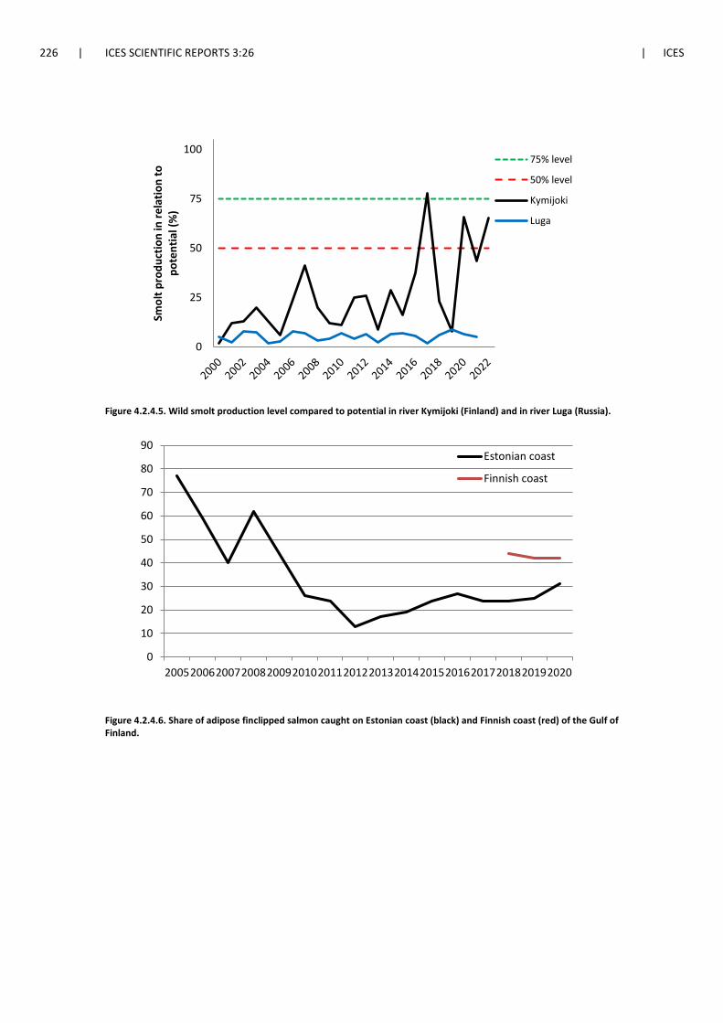
226 | ICES SCIENTIFIC REPORTS 3:26 | ICES
Figure 4.2.4.5. Wild smolt production level compared to potential in river Kymijoki (Finland) and in river Luga (Russia).
Figure 4.2.4.6. Share of adipose finclipped salmon caught on Estonian coast (black) and Finnish coast (red) of the Gulf of Finland.
0
25
50
75
100Sm
olt p
rodu
ctio
n in
rela
tion
to
pote
ntia
l (%
) 75% level
50% level
Kymijoki
Luga
0
10
20
30
40
50
60
70
80
90
2005200620072008200920102011201220132014201520162017201820192020
Estonian coast
Finnish coast
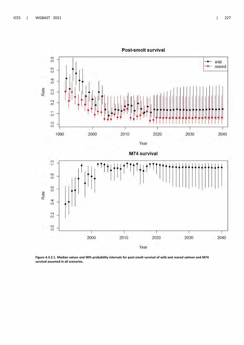
ICES | WGBAST 2021 | 227
Figure 4.3.2.1. Median values and 90% probability intervals for post-smolt survival of wild and reared salmon and M74 survival assumed in all scenarios.
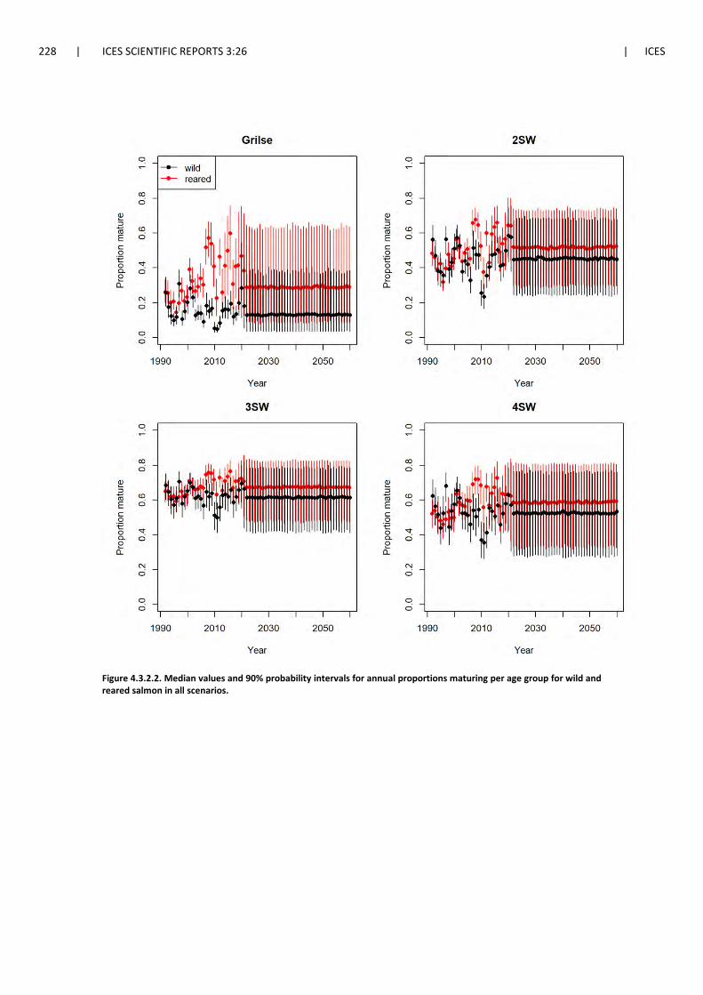
228 | ICES SCIENTIFIC REPORTS 3:26 | ICES
Figure 4.3.2.2. Median values and 90% probability intervals for annual proportions maturing per age group for wild and reared salmon in all scenarios.
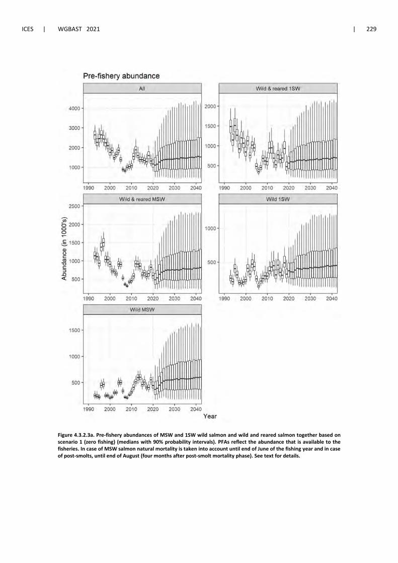
ICES | WGBAST 2021 | 229
Figure 4.3.2.3a. Pre-fishery abundances of MSW and 1SW wild salmon and wild and reared salmon together based on scenario 1 (zero fishing) (medians with 90% probability intervals). PFAs reflect the abundance that is available to the fisheries. In case of MSW salmon natural mortality is taken into account until end of June of the fishing year and in case of post-smolts, until end of August (four months after post-smolt mortality phase). See text for details.
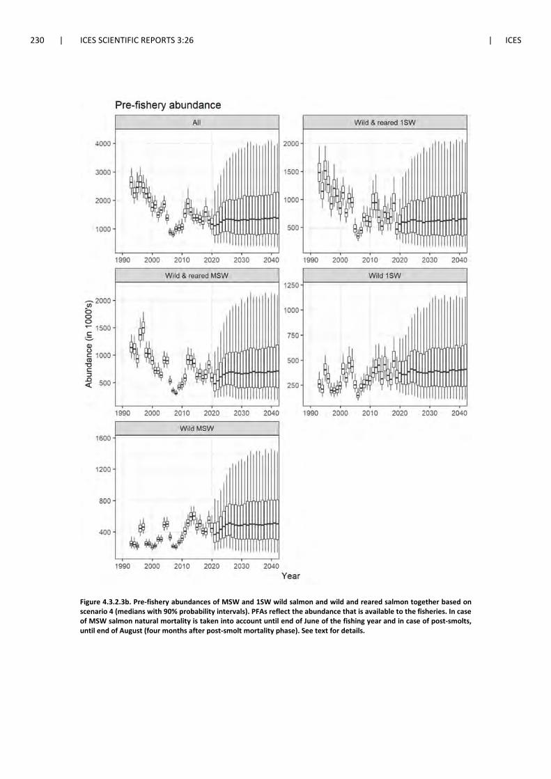
230 | ICES SCIENTIFIC REPORTS 3:26 | ICES
Figure 4.3.2.3b. Pre-fishery abundances of MSW and 1SW wild salmon and wild and reared salmon together based on scenario 4 (medians with 90% probability intervals). PFAs reflect the abundance that is available to the fisheries. In case of MSW salmon natural mortality is taken into account until end of June of the fishing year and in case of post-smolts, until end of August (four months after post-smolt mortality phase). See text for details.
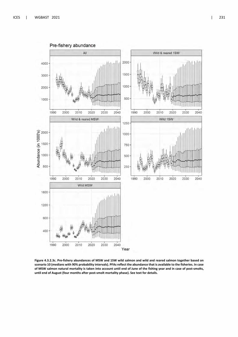
ICES | WGBAST 2021 | 231
Figure 4.3.2.3c. Pre-fishery abundances of MSW and 1SW wild salmon and wild and reared salmon together based on scenario 10 (medians with 90% probability intervals). PFAs reflect the abundance that is available to the fisheries. In case of MSW salmon natural mortality is taken into account until end of June of the fishing year and in case of post-smolts, until end of August (four months after post-smolt mortality phase). See text for details.
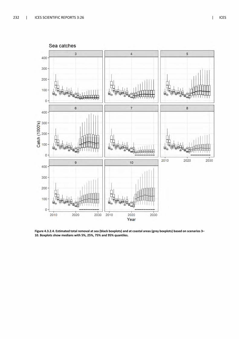
232 | ICES SCIENTIFIC REPORTS 3:26 | ICES
Figure 4.3.2.4. Estimated total removal at sea (black boxplots) and at coastal areas (grey boxplots) based on scenarios 3–10. Boxplots show medians with 5%, 25%, 75% and 95% quantiles.
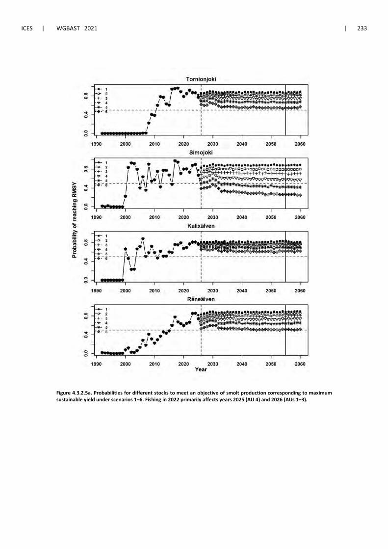
ICES | WGBAST 2021 | 233
Figure 4.3.2.5a. Probabilities for different stocks to meet an objective of smolt production corresponding to maximum sustainable yield under scenarios 1–6. Fishing in 2022 primarily affects years 2025 (AU 4) and 2026 (AUs 1–3).
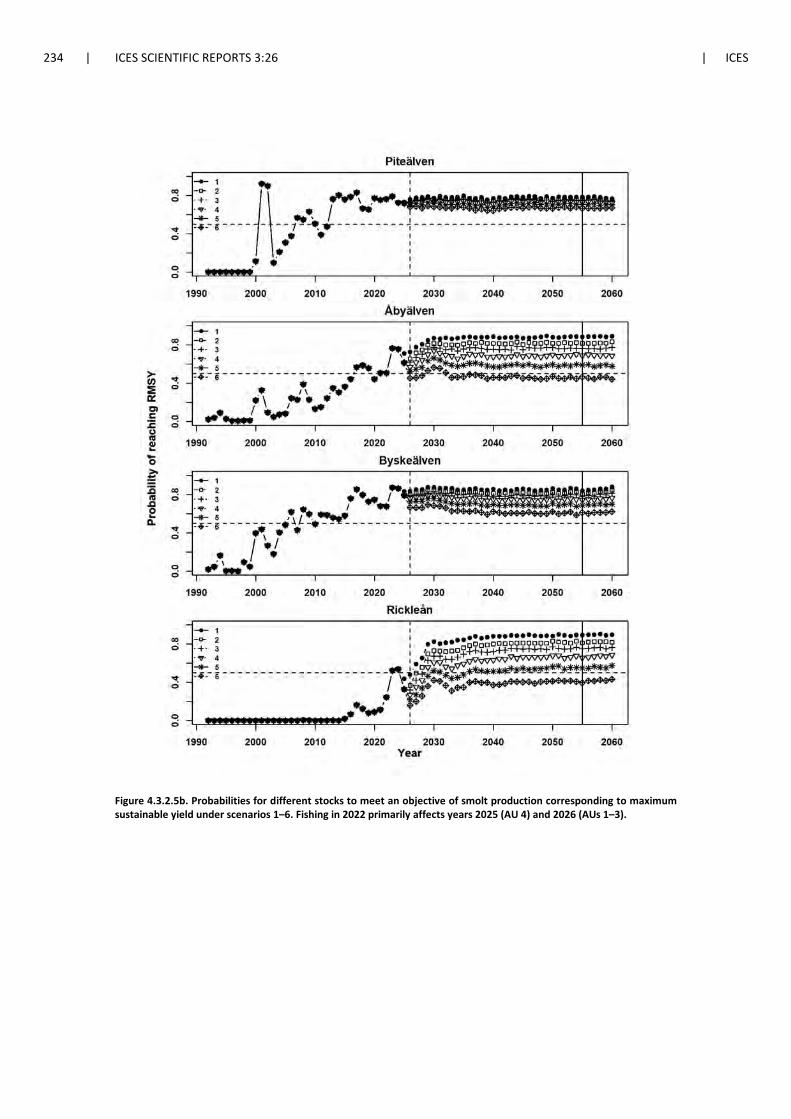
234 | ICES SCIENTIFIC REPORTS 3:26 | ICES
Figure 4.3.2.5b. Probabilities for different stocks to meet an objective of smolt production corresponding to maximum sustainable yield under scenarios 1–6. Fishing in 2022 primarily affects years 2025 (AU 4) and 2026 (AUs 1–3).
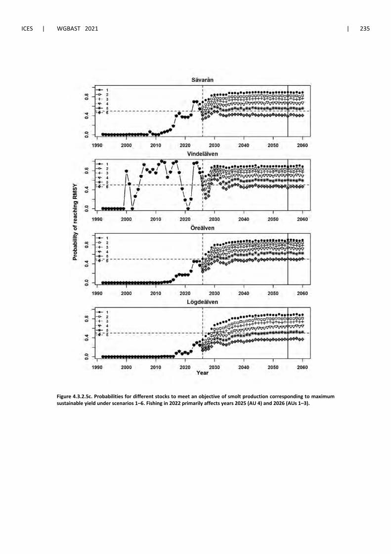
ICES | WGBAST 2021 | 235
Figure 4.3.2.5c. Probabilities for different stocks to meet an objective of smolt production corresponding to maximum sustainable yield under scenarios 1–6. Fishing in 2022 primarily affects years 2025 (AU 4) and 2026 (AUs 1–3).
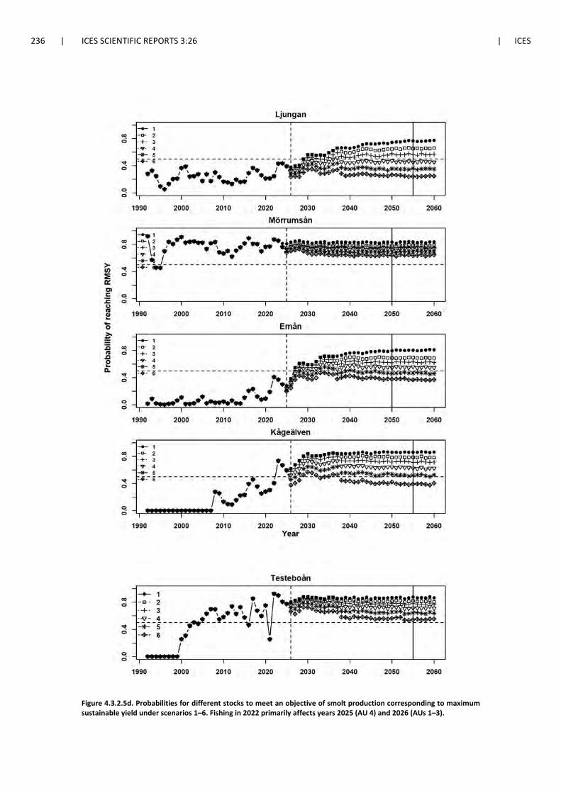
236 | ICES SCIENTIFIC REPORTS 3:26 | ICES
Figure 4.3.2.5d. Probabilities for different stocks to meet an objective of smolt production corresponding to maximum sustainable yield under scenarios 1–6. Fishing in 2022 primarily affects years 2025 (AU 4) and 2026 (AUs 1–3).
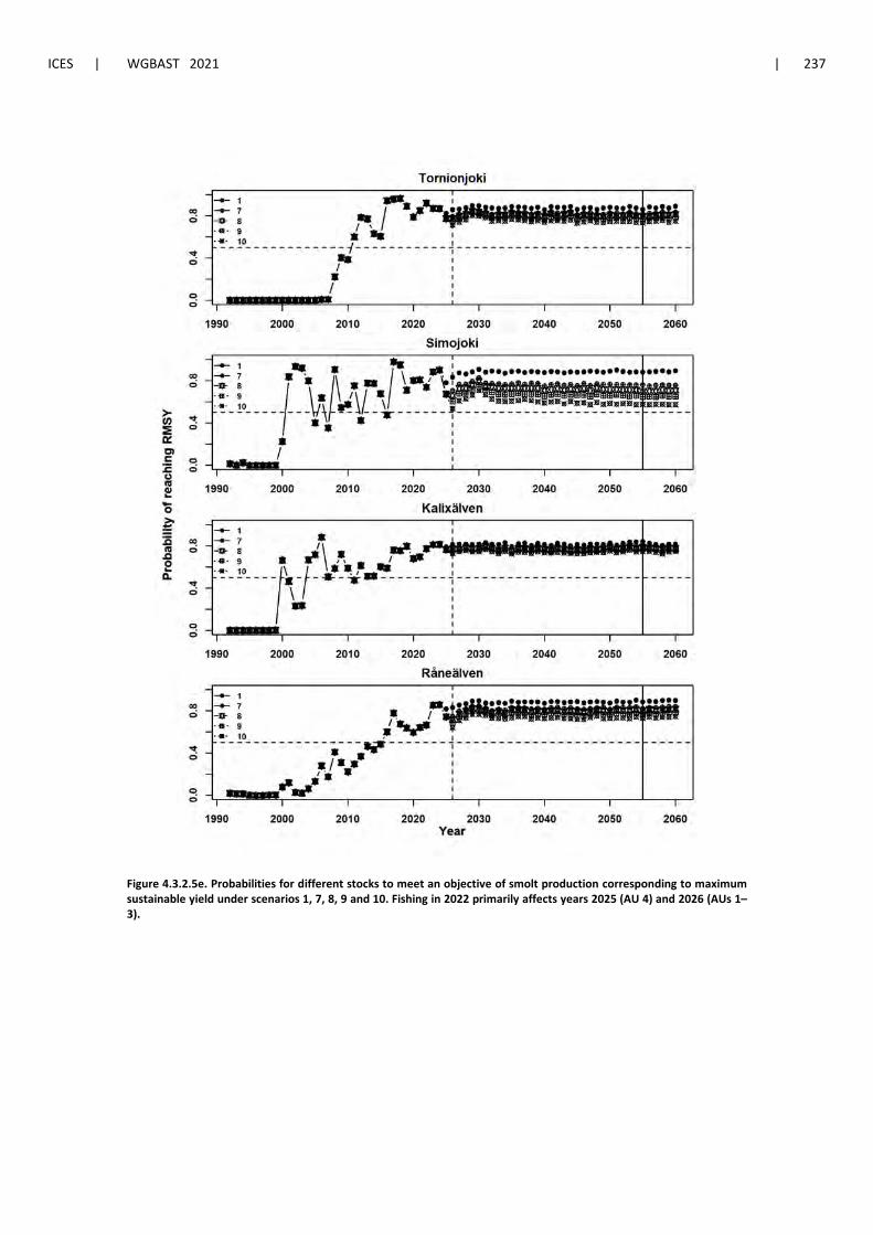
ICES | WGBAST 2021 | 237
Figure 4.3.2.5e. Probabilities for different stocks to meet an objective of smolt production corresponding to maximum sustainable yield under scenarios 1, 7, 8, 9 and 10. Fishing in 2022 primarily affects years 2025 (AU 4) and 2026 (AUs 1–3).
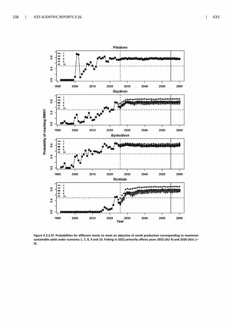
238 | ICES SCIENTIFIC REPORTS 3:26 | ICES
Figure 4.3.2.5f. Probabilities for different stocks to meet an objective of smolt production corresponding to maximum sustainable yield under scenarios 1, 7, 8, 9 and 10. Fishing in 2022 primarily affects years 2025 (AU 4) and 2026 (AUs 1–3).
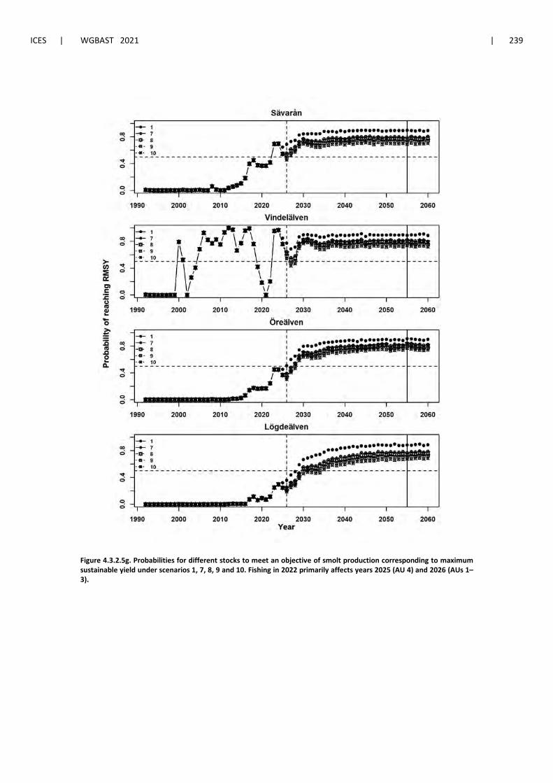
ICES | WGBAST 2021 | 239
Figure 4.3.2.5g. Probabilities for different stocks to meet an objective of smolt production corresponding to maximum sustainable yield under scenarios 1, 7, 8, 9 and 10. Fishing in 2022 primarily affects years 2025 (AU 4) and 2026 (AUs 1–3).
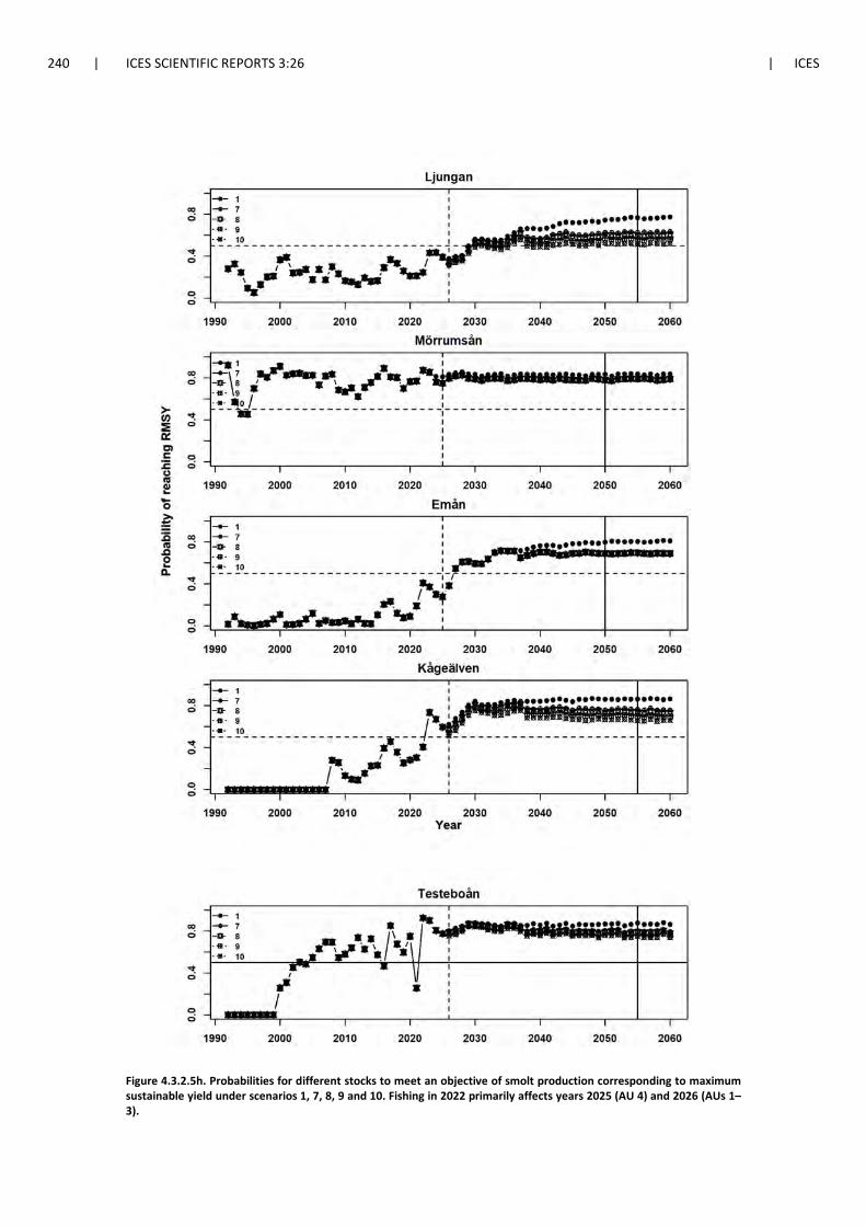
240 | ICES SCIENTIFIC REPORTS 3:26 | ICES
Figure 4.3.2.5h. Probabilities for different stocks to meet an objective of smolt production corresponding to maximum sustainable yield under scenarios 1, 7, 8, 9 and 10. Fishing in 2022 primarily affects years 2025 (AU 4) and 2026 (AUs 1–3).
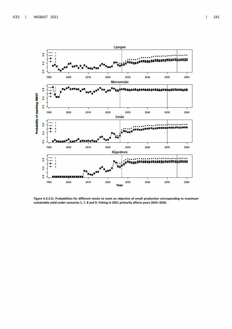
ICES | WGBAST 2021 | 241
Figure 4.3.2.5i. Probabilities for different stocks to meet an objective of smolt production corresponding to maximum sustainable yield under scenarios 1, 7, 8 and 9. Fishing in 2021 primarily affects years 2025–2026.
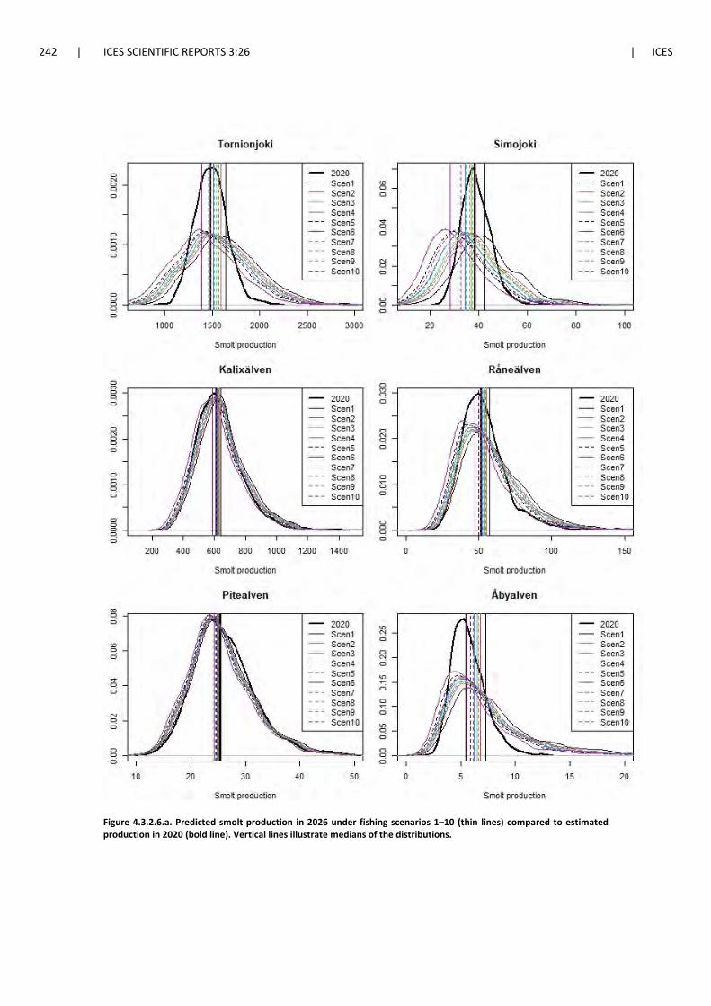
242 | ICES SCIENTIFIC REPORTS 3:26 | ICES
Figure 4.3.2.6.a. Predicted smolt production in 2026 under fishing scenarios 1–10 (thin lines) compared to estimated production in 2020 (bold line). Vertical lines illustrate medians of the distributions.
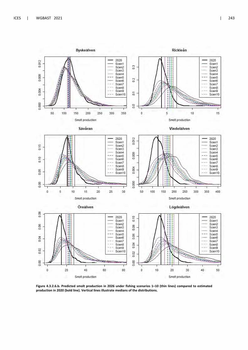
ICES | WGBAST 2021 | 243
Figure 4.3.2.6.b. Predicted smolt production in 2026 under fishing scenarios 1–10 (thin lines) compared to estimated production in 2020 (bold line). Vertical lines illustrate medians of the distributions.
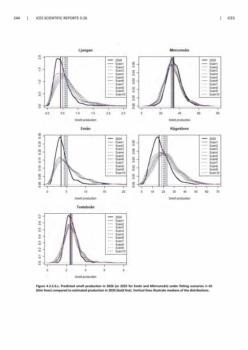
244 | ICES SCIENTIFIC REPORTS 3:26 | ICES
Figure 4.3.2.6.c. Predicted smolt production in 2026 (or 2025 for Emån and Mörrumsån) under fishing scenarios 1–10 (thin lines) compared to estimated production in 2020 (bold line). Vertical lines illustrate medians of the distributions.
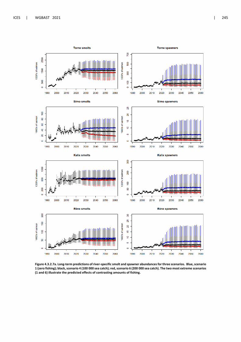
ICES | WGBAST 2021 | 245
Figure 4.3.2.7a. Long-term predictions of river-specific smolt and spawner abundances for three scenarios. Blue, scenario 1 (zero fishing); black, scenario 4 (100 000 sea catch); red, scenario 6 (200 000 sea catch). The two most extreme scenarios (1 and 6) illustrate the predicted effects of contrasting amounts of fishing.
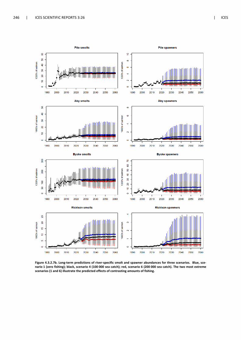
246 | ICES SCIENTIFIC REPORTS 3:26 | ICES
Figure 4.3.2.7b. Long-term predictions of river-specific smolt and spawner abundances for three scenarios. Blue, sce-nario 1 (zero fishing); black, scenario 4 (100 000 sea catch); red, scenario 6 (200 000 sea catch). The two most extreme scenarios (1 and 6) illustrate the predicted effects of contrasting amounts of fishing.
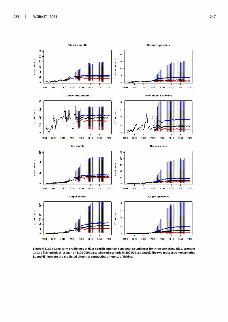
ICES | WGBAST 2021 | 247
Figure 4.3.2.7c. Long-term predictions of river-specific smolt and spawner abundances for three scenarios. Blue, scenario 1 (zero fishing); black, scenario 4 (100 000 sea catch); red, scenario 6 (200 000 sea catch). The two most extreme scenarios (1 and 6) illustrate the predicted effects of contrasting amounts of fishing.
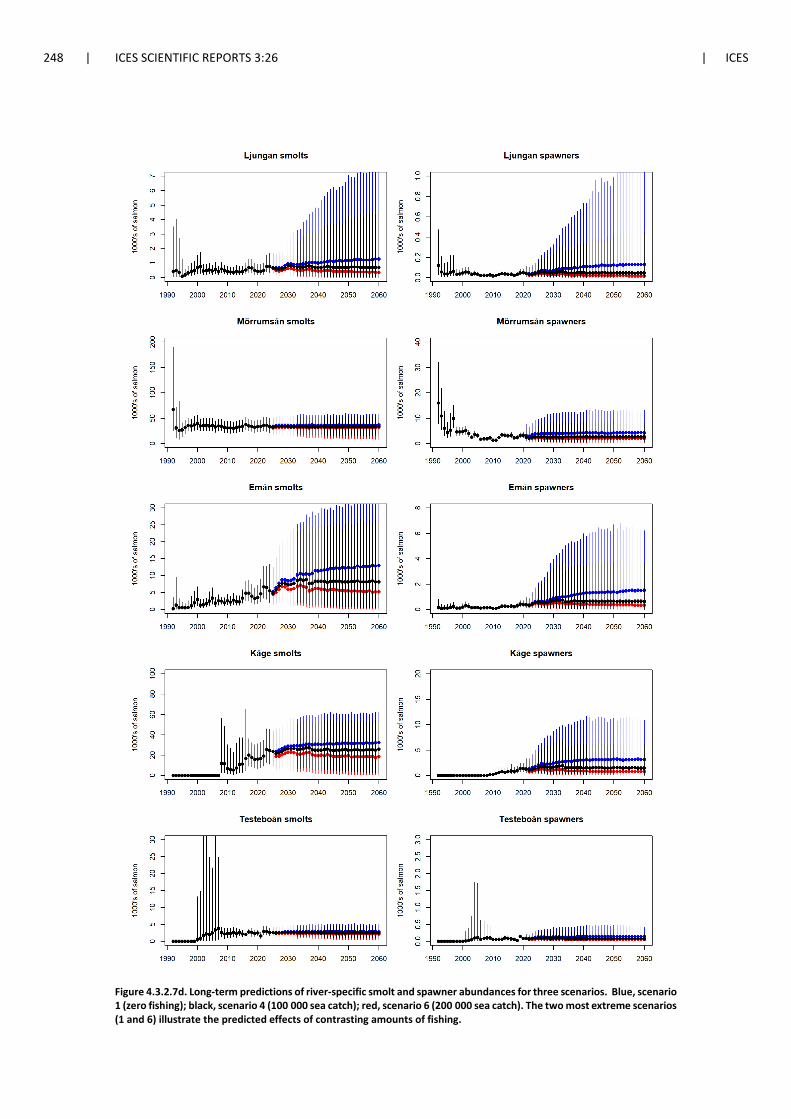
248 | ICES SCIENTIFIC REPORTS 3:26 | ICES
Figure 4.3.2.7d. Long-term predictions of river-specific smolt and spawner abundances for three scenarios. Blue, scenario 1 (zero fishing); black, scenario 4 (100 000 sea catch); red, scenario 6 (200 000 sea catch). The two most extreme scenarios (1 and 6) illustrate the predicted effects of contrasting amounts of fishing.
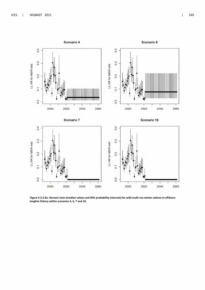
ICES | WGBAST 2021 | 249
Figure 4.3.2.8a. Harvest rates (median values and 90% probability intervals) for wild multi-sea winter salmon in offshore longline fishery within scenarios 4, 6, 7 and 10.
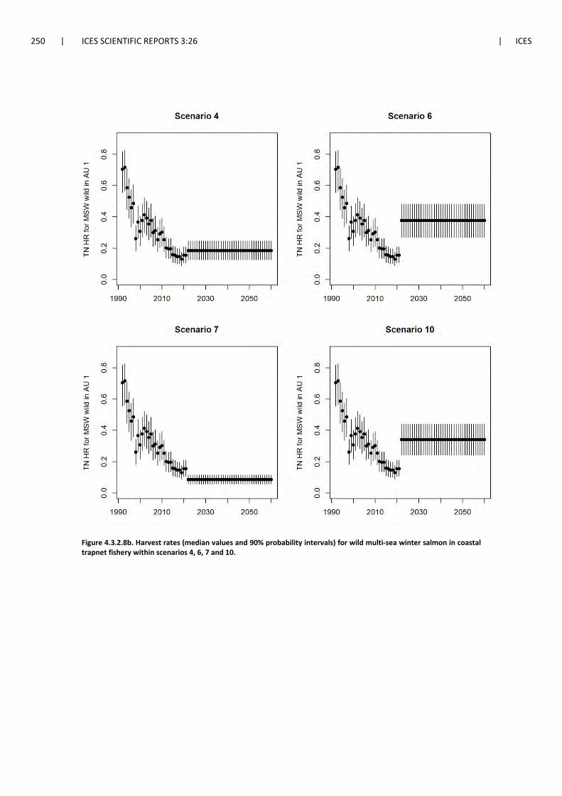
250 | ICES SCIENTIFIC REPORTS 3:26 | ICES
Figure 4.3.2.8b. Harvest rates (median values and 90% probability intervals) for wild multi-sea winter salmon in coastal trapnet fishery within scenarios 4, 6, 7 and 10.
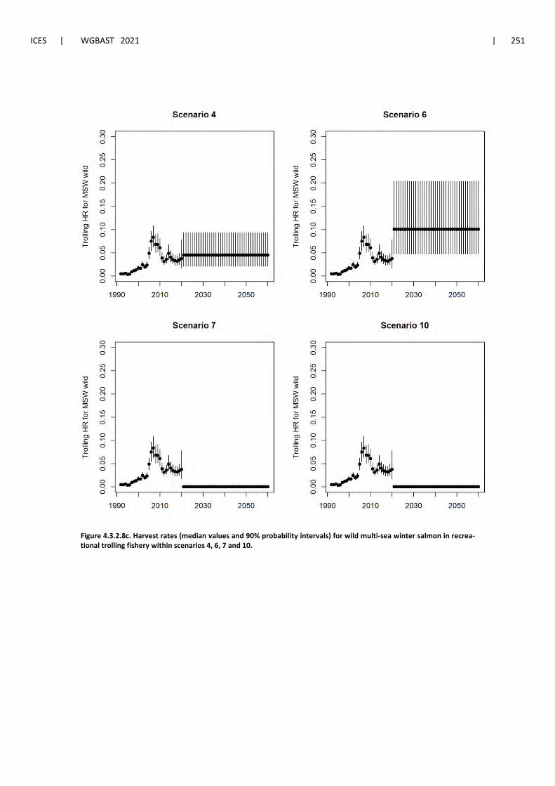
ICES | WGBAST 2021 | 251
Figure 4.3.2.8c. Harvest rates (median values and 90% probability intervals) for wild multi-sea winter salmon in recrea-tional trolling fishery within scenarios 4, 6, 7 and 10.
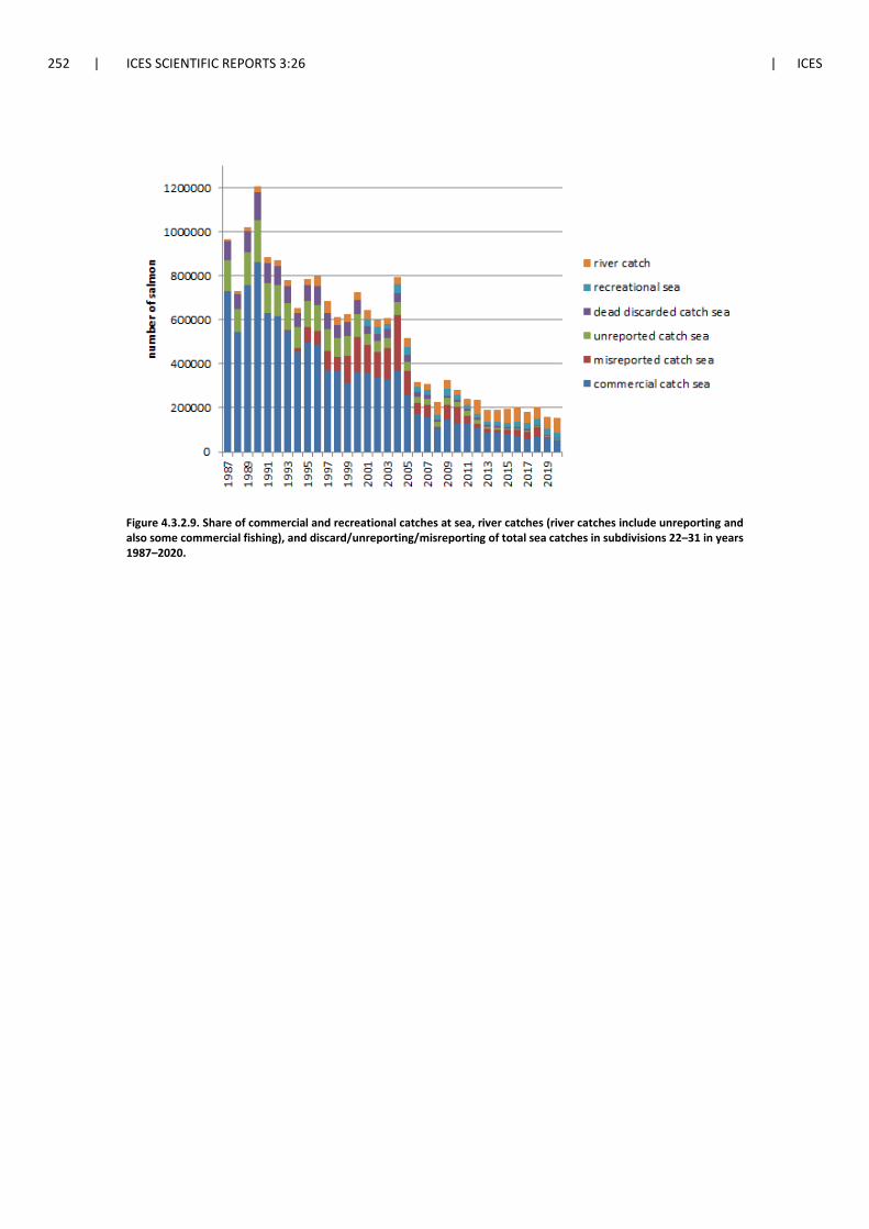
252 | ICES SCIENTIFIC REPORTS 3:26 | ICES
Figure 4.3.2.9. Share of commercial and recreational catches at sea, river catches (river catches include unreporting and also some commercial fishing), and discard/unreporting/misreporting of total sea catches in subdivisions 22–31 in years 1987–2020.
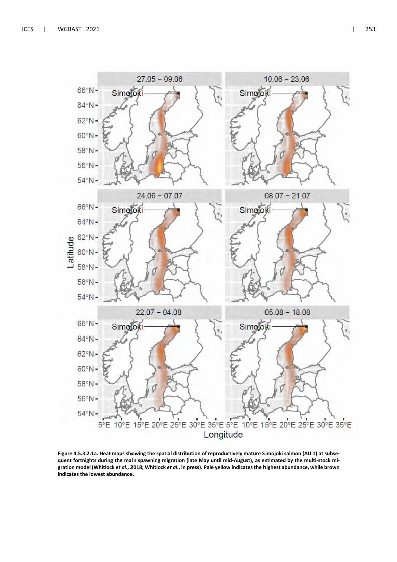
ICES | WGBAST 2021 | 253
Figure 4.5.3.2.1a. Heat maps showing the spatial distribution of reproductively mature Simojoki salmon (AU 1) at subse-quent fortnights during the main spawning migration (late May until mid-August), as estimated by the multi-stock mi-gration model (Whitlock et al., 2018; Whitlock et al., in press). Pale yellow indicates the highest abundance, while brown indicates the lowest abundance.
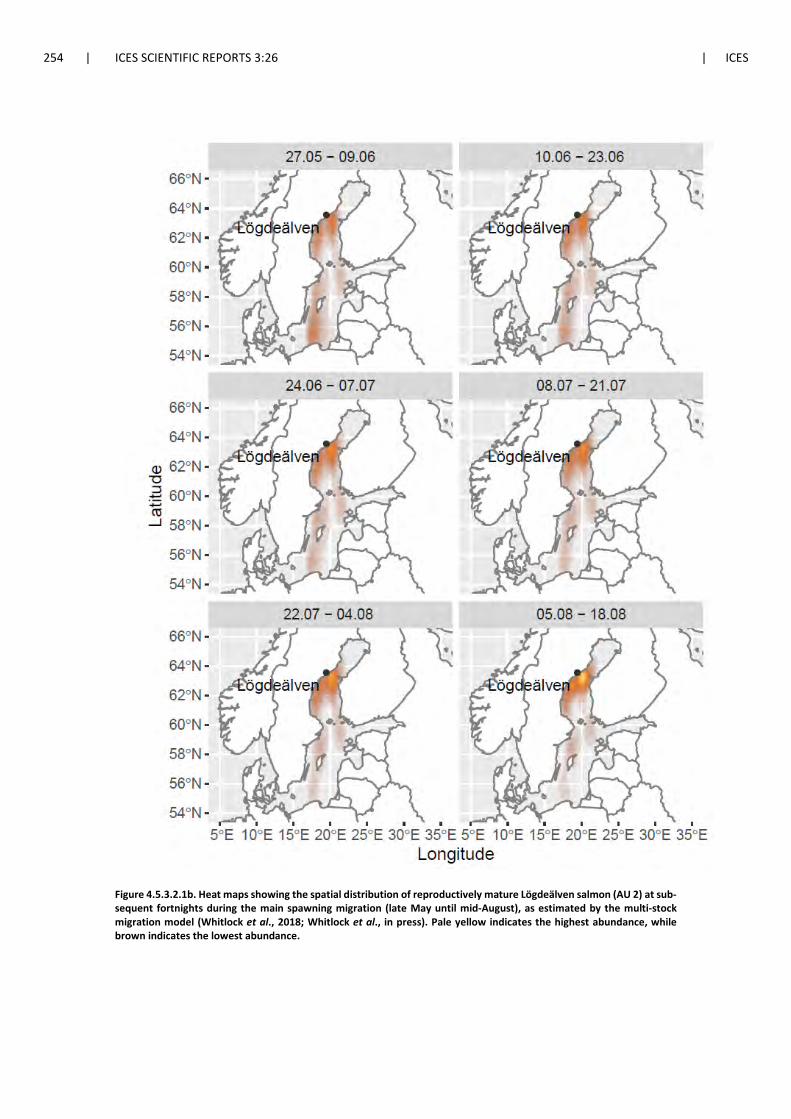
254 | ICES SCIENTIFIC REPORTS 3:26 | ICES
Figure 4.5.3.2.1b. Heat maps showing the spatial distribution of reproductively mature Lögdeälven salmon (AU 2) at sub-sequent fortnights during the main spawning migration (late May until mid-August), as estimated by the multi-stock migration model (Whitlock et al., 2018; Whitlock et al., in press). Pale yellow indicates the highest abundance, while brown indicates the lowest abundance.
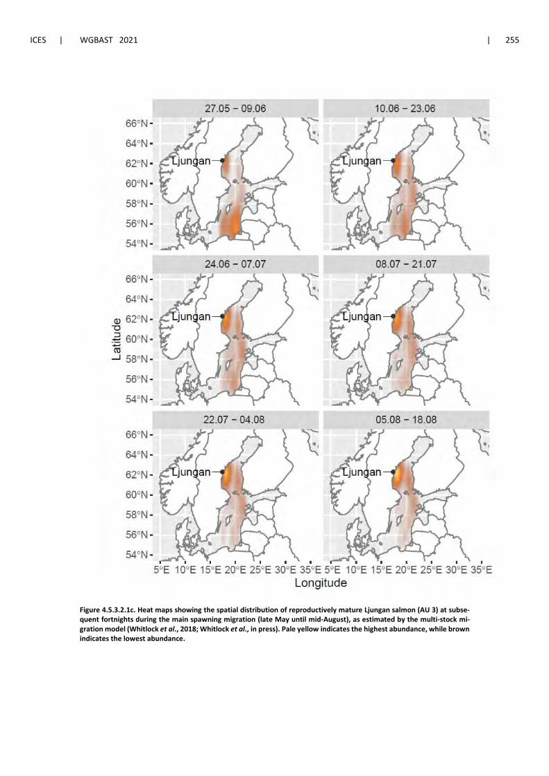
ICES | WGBAST 2021 | 255
Figure 4.5.3.2.1c. Heat maps showing the spatial distribution of reproductively mature Ljungan salmon (AU 3) at subse-quent fortnights during the main spawning migration (late May until mid-August), as estimated by the multi-stock mi-gration model (Whitlock et al., 2018; Whitlock et al., in press). Pale yellow indicates the highest abundance, while brown indicates the lowest abundance.
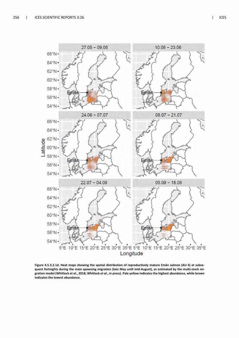
256 | ICES SCIENTIFIC REPORTS 3:26 | ICES
Figure 4.5.3.2.1d. Heat maps showing the spatial distribution of reproductively mature Emån salmon (AU 4) at subse-quent fortnights during the main spawning migration (late May until mid-August), as estimated by the multi-stock mi-gration model (Whitlock et al., 2018; Whitlock et al., in press). Pale yellow indicates the highest abundance, while brown indicates the lowest abundance.
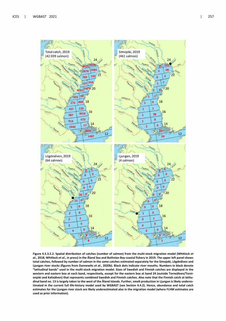
ICES | WGBAST 2021 | 257
Figure 4.5.3.2.2. Spatial distribution of catches (number of salmon) from the multi-stock migration model (Whitlock et al., 2018; Whitlock et al., in press) in the Åland Sea and Bothnian Bay coastal fishery in 2019. The upper left panel shows total catches, followed by number of salmon in the same catches estimated separately for the Simojoki, Lögdeälven and Ljungan river stocks (figures from Dannewitz et al., 2020b). Black dots indicate river mouths. Numbers in black denote “latitudinal bands” used in the multi-stock migration model. Sizes of Swedish and Finnish catches are displayed in the western and eastern box at each band, respectively, except for the eastern box at band 24 (outside Torneälven/Torni-onjoki and Kalixälven) that represents combined Swedish and Finnish catches. Also note that the Finnish catch at latitu-dinal band no. 13 is largely taken to the west of the Åland Islands. Further, smolt production in Ljungan is likely underes-timated in the current full life-history model used by WGBAST (see Section 4.4.2). Hence, abundance and total catch estimates for the Ljungan river stock are likely underestimated also in the migration model (where FLHM estimates are used as prior information).
260 | ICES SCIENTIFIC REPORTS 3:26 | ICES
5 Sea trout
Sea trout basically has the same life cycle as salmon. The most important difference is that most strains do not migrate as far as the salmon. Instead, they spend the time at sea in coastal waters where the majority of sea trout from a specific strain stay within a few hundred kilometres from their home river. Some specimens, however, migrate further and in some strains in the Southern Baltic, most sea trout seem to migrate longer distances into the open sea. Sea trout spawn and live during the first period of life in smaller streams than salmon. In the Baltic Sea area, sea trout are found in a much larger number of streams than salmon.
The assessment of sea trout populations in the Baltic is partly based on a model developed by the Study Group on Data Requirements and Assessment Needs for Baltic Sea Trout, SGBAL-ANST (ICES, 2011), first implemented at the assessment in 2012 (ICES, 2012). For the evaluation of model results, other basic observations such as tagging data, count of spawners and catch statistics are also taken into account.
Below follows subsections on sea trout catches, fisheries, and biological monitoring data fol-lowed by descriptions of assessment methods and results.
5.1 Baltic Sea trout catches
5.1.1 Commercial fisheries
Nominal commercial catches of sea trout in the Baltic Sea are presented in Table 5.1.1.1. The total catch was slightly lower than in last year and amounted to 148 tonnes in 2020. A majority (80%) of this catch was caught in the Main Basin.
In the Main Basin, the catch decreased from 954 tonnes in 2002 to 236 tonnes in 2008. After two years (2009–2010) of somewhat higher catches, around 450 tonnes, the total commercial catch again fell, reaching a minimum of 145 tonnes in 2015. In 2016, the total Main Basin commercial catch again increased somewhat to 184 tonnes (where it remained in 2017) and in 2018, it in-creased further to 274 tonnes. In 2019, catches decreased here about 45% and reached only 123 tonnes. As in previous years, the majority of this catch was from the Polish fishery (74%). In 2020 catches were slightly lower than in 2019 and amounted to 116 tonnes.
The total nominal commercial catch of trout in the Gulf of Bothnia was 19 tonnes in 2019, which is similar to 2018 (22 tonnes) and below the ten-year average catch (46 tonnes). In 2020, the level of catches decreased slightly to 16 tonnes. All commercial catches in Gulf of Bothnia were from coastal fisheries.
In the Gulf of Finland, the total commercial sea trout catch in 2019 was 17 tonnes (Table 5.1.1.1), which is below the average for the last ten years (21 tonnes). In 2020, catches was similar to the previous year and amounted to 16 tonnes.
5.1.2 Recreational fisheries
Recreational sea trout catches (landed) in the Baltic Sea are presented in Table 5.1.2.1. In 2020, the total catch increased to 656 tonnes, from 589 tonnes in 2019. However, the catch was lower than in 2016–2017 when about 750 tonnes were reported. A majority (85%) of this catch was caught in the Main Basin.
ICES | WGBAST 2021 | 261
Recreational river catches in 2020 were 37 tonnes, and were taken mainly in Swedish Gulf of Bothnia rivers. This is a smaller river catch than the ten years average (43 tonnes; Table 5.1.2.1). Most of the recreational catch in the coastal zones of the Gulf of Bothnia and the Gulf of Finland was taken by Finnish fishermen (64 tonnes), similar to the last years.
Data on recreational coastal catches from the Main Basin in 2018 were available from Estonia, Latvia, Lithuania, Finland, Poland, Sweden and partially from Denmark and Germany (Table 5.1.2.1). From the last several years, results from questionnaires on Danish that coastal recrea-tional catches increased from 224 tonnes in 2011 to 521 tonnes in 2014. Until 2016, they decreased to 323 tonnes, which constituted about 55% of the total Baltic Sea recreational catch of sea trout. In 2017–2019 this share is lower (about 30–40%). In the current year, the data have been upgraded with the results of Polish recreational sea fishing for 2017–2020 years.
5.1.3 Total nominal catches
The highest combined commercial and recreational nominal catches, above 1300 tonnes, were taken in the early and late 1990s (Table 5.1.3.1). Since 2001, they have been decreasing to the level of 700–800 tonnes in recent years (Tables 5.1.1.1 and 5.1.2.1 combined). In 2020, the combined catch reached 804 tonnes, and was higher by approximately 40% than in 2019. Note that when taking estimated levels of misreporting of salmon as sea trout in the Polish sea fishery into ac-count (Section 2.3.3), the overall reported commercial sea trout catches have been much too high. However, in last year, according to new regulation in Polish fisheries, the level of misreported catch has dropped almost to zero. This situation continued in 2020. A column with yearly esti-mates of salmon catches misreported as sea trout (in weight) in the last ten years were added to Table 5.1.1.1.
5.1.4 Biological catch sampling
Strategies for biological sampling of sea trout and procedures are very similar to those for salmon (Annex 2, Section 2.5). In total, 1424 sea trout were sampled in 2020, similar to in 2019 (Table 5.1.4.1). Most samples were collected from Latvian (n=716) and Swedish (n=243) catches. In ad-dition, 150 samples were collected from Estonian catches in the Gulf of Finland (SD 32), and 95 from Finnish catches in SD 29–32. Polish samples originated from river catches (n=100) in the Rega River and from the sea (n=27). Additionally, 25 sea trout were sampled in Germany and only four in Lithuania.
5.2 Data collection and methods
5.2.1 Monitoring methods
Monitoring of sea trout populations is carried out in all Baltic Sea countries. The intensity and period during which monitoring has been going on varies (ICES, 2008c). Some countries started their monitoring in recent years, while very long dataseries exist for a few streams in others (ICES, 2008c). From 2016, a new European Union (EU) regulation (2016/1251) adopting a multi-annual program for the collection, management and use of data in the fisheries and aquaculture, obligated EU countries to collect sea trout catch data.
Most monitoring of sea trout is carried out by surveying densities of trout parr in nursery streams by electrofishing. In Denmark, only a few sites in Baltic streams are monitored annually. In ad-dition, a rolling scheme is used for electrofishing-monitoring of sea trout on the national level. Due to the large time lap between fishing separate rivers these are not directly useable for
262 | ICES SCIENTIFIC REPORTS 3:26 | ICES
assessment, but the results are used as background information on the status of populations as such. In a couple of countries, sampling of parr densities are used to calculate smolt production by a relation of parr to smolt survival, either developed in the same stream or in some other (ICES, 2008a). In most countries (but not in Denmark and Poland) electrofishing is supplemented with annual monitoring of smolt escapement by trapping and counting in one or more streams. In total, smolt production estimates exist for 12–13 rivers in the entire Baltic area, but the length of the time-series varies very much.
In only three streams/rivers (Mörrumsån and Testeboån in Sweden and Pirita in Estonia) both numbers of spawners and smolts are monitored. Adult counts are determined by trapping or recording of ascending sea trout using automatic counters. In 24 rivers (nine in Sweden, three in Poland, eight in Germany, one in Estonia and three in Finland) the numbers of spawners are monitored by automatic fish counters or video systems. In three rivers, the total run of salmonids is determined using echosounder systems. However, this technique does not allow strict dis-crimination between sea trout and salmon (or other fish species of similar size).
An indication of the spawning intensity can also be obtained by counting of redds. Such infor-mation is collected from a number of sea trout streams in Poland, Lithuania and Germany (ICES, 2008a). In a couple of streams in Denmark, the catch in sports fisheries has been used to estimate the development of the spawning run. Catch numbers are also available from some Swedish rivers. Tagging and marking are furthermore used as methods to obtain quantitative and quali-tative information on trout populations (see below). Evaluation of sea trout status in rivers is done based on national expert opinions, as well as on factors influencing status. Such evaluations are updated irregularly.
5.2.2 Assessment of recreational sea trout fisheries
There is a highly developed recreational fishery targeting sea trout in many countries. Angling (rod-and-line fishing) accounts for the majority of the catches. The most common methods are spin and fly fishing from the shore or in rivers, and trolling with small boats at sea. The shore-based fishery along coasts and in rivers is highly diffuse and variable with strong local and re-gional variations depending on weather conditions and season. In the southern Baltic Sea, recre-ational fishing on sea trout takes places during the whole year with distinct activity peaks in spring and autumn, some night fishing occurs in summer.
While the recreational catches of sea trout are largely dominated by rod-and-line fisheries, there are other types of fisheries carried out in some countries. To a smaller extent passive gears such as trapnets, gillnets or longlines are being used for catching sea trout, either as a target species or as bycatch in other coastal recreational fisheries. Except for in northern Gulf of Bothnia, the catches from this type of fishing is estimated to be of minor importance in terms of impact on the stocks, i.e. removals.
Monitoring of the recreational fisheries is carried out in different ways. Below follows a descrip-tion of methods and activities in the Baltic countries.
Since 2009, recreational catches of sea trout in Denmark have been estimated based on an inter-view-based recall survey, which is conducted by DTU Aqua in cooperation with Statistics Den-mark. Information is collected two times per year. In addition, during spring 2017, a project on the recreational sea trout coastal rod-and-line fishery was carried out on the island Funen in SD 22. Two different approaches were applied: 1) on-site interviews (rowing creel) collected infor-mation on i.a. catch, release rates and effort, and 2) by aerial survey, information on effort was obtained. Furthermore, information on motivation and satisfaction was collected.
ICES | WGBAST 2021 | 263
In Estonia, catch reporting has been mandatory since 2005. The data are reported to and stored in the Estonian Fisheries Information System (EFIS) for passive gears (gillnets, longlines) and salmon and sea trout rod-and-line fishing in rivers. The latest recreational fishery survey was carried out in 2016, based on a phone call approach.
Since 2002, the official catch estimates of the recreational sea trout fishery in Finland are based on a national recreational fisheries survey. Biannual surveys are conducted to estimate partici-pation, fishing effort and catches of the recreational fishery (http://stat.luke.fi/en/recreational-fishing). A stratified sample of about 7500 household dwellings is contacted with response rates of around 40–45% after a maximum of three contacts. Afterwards, a telephone interview is done for a sample of the non-respondents. Harvested and released catch is measured separately by species. The latest estimate of recreational sea trout catch is for 2018 year and being 64 (CV>50%) tonnes. Due to methodical reasons, the catch estimate varies significantly between the recent and older surveys. Other information, however, does not indicate such a large variation in the true catches between the years. In the WGBAST catch data, the Finnish recreational catch estimates before the year 2002 is relative to the commercial catch by assumption that recreational catch constituted about 75% (derived from the tag return data) of the total catch (re-evaluation is con-sidered). Since year 2002, the estimates have been based on the Finnish Recreational Fishing Sur-vey results. The 2020 survey is ongoing and results will be published in October 2021.
In Germany, a nationwide telephone-diary survey with quarterly follow-ups was conducted in 2014/2015, contacting 50 000 German households to collect representative data on catch and ef-fort, and social, economic and demographic parameters for the German marine recreational fish-ery, covering also the recreational sea trout fishery. However, to collect more detailed infor-mation on the recreational sea trout fishery an additional pilot study (diary recall survey) was conducted. During this study, a bus route intercept survey was used to recruit diarists, collect biological samples (length, weight, scales, and tissue samples), and socio-economic data. Ongo-ing analyses aim to combine both studies to provide a full picture of the recreational sea trout fishery in Germany. Anecdotal information showed that recreational sea trout catches in fresh-water are small and probably insignificant compared to marine catches. The results of the survey conducted in 2015 were considered to be a reliable level of recreational fishing and their result (151 tonnes) was also adopted for the years 2016–2019. An update of the recreational sea trout catches is expected to be available in 2021.
In Latvia, a first attempt to estimate total sea trout catches from angling was done in 2018 using Internet questionnaires. The main aim was to get general information about angling places, gears and efforts. In a second part of the questionnaire, information about sea trout, salmon, cod and eel catches were collected. The total estimate received of sea trout caught in the recreational fish-ery was deemed highly unrealistic, amounting to 51 978 individuals (156 tons), and should not be used in further analyses. Sea trout angling from coast is not popular in Latvia due to an unfa-vourable coastline (most of the coast consists of sandy beaches, no islands or archipelagos) and ice coverage in winter. However, all landings in the Latvian “self-consumption fishery” are re-ported in logbooks. According to this logbook information landings of seatrout in 2018 were 1957 individuals. Additionally, according to official reports from the licensed fishery, 103 sea trout were caught. This estimate does not include angling in Daugava River (no licensing, because Daugava stock consists mainly from reared salmon and sea trout) or angling from the coast. In 2019 recreational coastal (1277), recreational offshore (10) and river angling (172) landed 1459 sea trout. In the rivers, where natural reproduction of salmon occurs, all angling and fishing for salmon and sea trout is prohibited with exception of licensed angling for sea trout and salmon kelts during the spring season. This encompass the rivers Salaca, Venta and from 2020 also Gauja River. In total, 772 retained sea trout kelts were reported in licensed angling in 2020. The large increase in reported retained salmon and sea trout in the Salaca River can be explained by more active and accurate data registration and submission. Submission of data has improved due to
264 | ICES SCIENTIFIC REPORTS 3:26 | ICES
amendments to the rules of licensed angling – anglers cannot buy a new licence without submit-ting a report about previous one.
In Lithuania, recreational sea trout fishing is mainly conducted in rivers. Since 2015, recreational (anglers) sea trout catches are estimated by an online survey, a face-to-face interview survey, and individual interviews and catch reporting with diaries of selected anglers and experts. CPUE data (ind/person/day) are estimated from survey data, and combined with number of licences sold to anglers to calculate the total catch. In 2015, the online survey, face-to-face interview sur-vey, and individual angler interviews were conducted, whereas in 2016 and 2017 only online surveys were carried out.
Pilot study relating to salmon and sea trout recreational fisheries was conducted in 2017–2019. Based on the results of the pilot study, sampling programme was included into regular sampling since 2020. In 2020, trolling boats have been observed in ten harbours with particular importance of Hel, Gdynia, Gdańsk Górki Zachodnie, Kołobrzeg harbours. A total of 125 different active trolling boats had been inventoried in 2020. Number of active trolling boats varied between au-tumn/winter (87–94) and spring (103–107) seasons with a higher number of trolling boats in spring. Because of COVID-19 issue, the catches have been affected by lower activity of trolling anglers, and national restrictions (lock-down). It is planned to update catch data for 2018–2020, based on obtained results. The estimated sea trout by-catch during salmon trolling trips in 2020 is 132 individuals (retained). The coastal sea trout catch estimates including coastal trolling tar-geting sea trout for 2020 was 81 713 fish.
A pilot study of estimation of Polish river recreational catches has begun in 2017 and was con-tinued in next three years. First on three rives: Ina (SD 24), Rega and Słupia (SD 25) and from 2018 also on Parsęta River (SD 25). In 2020 three new rivers were added to the survey: Łeba, Reda (SD 25) and Drwęca River (SD 26). The method used is based on catch records provided by fish-ing users supplemented with data from on-site surveys of anglers carried out according to the same schedule on the rivers studied. The data obtained from the catch records are delayed by two years, which results from the fishing fee system. The results obtained with the method de-veloped in the pilot study indicate that in 2018, 2330 sea trout were caught in the seven analysed rivers, which, assuming an average weight of 3 kg of sea trout, gives about 7 tons.
Results from on-site surveys performed in 2017–2020 show that the average catch per angler ranged from 0.9 sea trout (2016–2017) to 2.9 for (2019–2020) per year. It was also observed that these values were higher for the Parsęta River. In 2020, the average number of fishing occasions per respondent was 28. The vast majority of surveys were for local anglers. According to the questionnaire, half of the surveyed anglers prefer to practise catch and release. It has also been shown, that periods of intensity of sea trout fishing can vary significantly between rivers. In the Ina, Rega and Łeba rivers, the main fishing season is winter, while the rest of the fishing season is spread over time with peak just before spawning.
There are about ten rivers with similar intensity of sea trout/salmon fishing in Poland, so, taking into consideration underestimation of registers, recreational catch in Polish rivers can be roughly estimated for 40–80 specimens of salmon and 5–10 tons of sea trout yearly. As a result of the pilot study a method for catches estimation on main sea trout rivers was proposed. Based on the pro-posed method, it is planned to upgrade river catch data for earlier years in 2021.
In Russia, sea trout was previously a protected species in the Baltic Sea, and recreational fishers were not allowed to target sea trout in the sea nor in rivers. As from March 2020, sea trout fishing was allowed, but statistics for the catch have not been available.
In Sweden, recreational fishery for sea trout is very popular. Since there is no commercial fishing specifically targeting the species, commercial catches are low and most catches are from recrea-tional fisheries. A major part of the Swedish recreational catch is taken along the Baltic coast
ICES | WGBAST 2021 | 265
(>2400 km, including islands of Öland and Gotland), in particular by angling from shore or small boats, and from use of gillnets. Offshore recreational fisheries are in most cases done by trolling targeting salmon, with sea trout caught only occasionally. However, trolling closer to the coast targeting sea trout is starting to be popular in some areas. Swedish data on recreational sea trout river catches are almost only collected in larger salmon rivers, and therefore river catch statistics are far from complete. However, as mentioned, the largest proportion of the catch is assumed to be taken in coastal waters where no surveys specifically targeting sea trout are in place so far. Currently the best source for catch statistics comes from an annual national mail survey con-ducted by the Swedish Agency for Marine and Water Management (SWaM), the authority re-sponsible for fisheries management. The survey is sent to about 17 000 randomly selected per-sons each year, and it collects statistics on different aspects of recreational fishing (catches, ex-penditures, fishing days, etc.) for all species. However, this survey can neither estimate trout catches with good precision nor on the geographic scale needed for effective management. To obtain catch statistics with better precision and finer geographic resolution, a specific survey programme needs to be developed.
5.2.3 Marking and tagging
The total number of finclipped sea trout released in 2020 in the Baltic Sea area was 1 328 632 smolts and 33 045 parr, similar to the previous year (Table 5.2.2.1). Finclipping of hatchery-reared smolts is mandatory in Sweden, Finland and Estonia. The largest number of finclipped smolts was released in Sweden (598 760) followed by Latvia (369 972) and Finland (359 400). All released sea trout smolts have been finclipped in the Gulf of Finland since 2014 and in the Gulf of Bothnia since 2016. Finclipping was not performed in Poland in 2020, and stocked sea trout smolt were not finclipped in Denmark, Germany, Russia, Estonia or Lithuania. In 2020, the total number of Carlin tagged sea trout was only 2000 all released in Subdivision 31 (Table 5.2.2.1). The number of sea trout tagged with passive integrated transponders (PIT) increases every year. In 2020, 19 520 sea trout were tagged internally; the majority was tagged by Poland and Sweden as reared smolts. Polish smolt were released in the Vistula basin (6000) in Subdivision 26 and into the Parseta River (5000 smolts, SD 25). In subdivisions 31 and 30, smolts tagged with PITs were stocked in rivers Umeälven (2000) and Dalälven (6520) (Table 5.2.2.1). In Finland 511 700 eyed egg and fry of sea trout were marked with Alizarin Red Staining solution and released in subdi-visions 29–31 (Table 5.2.2.1).
5.3 Assessment of recruitment status
5.3.1 Methods
Recruitment status The SGBALANST (ICES, 2008c; 2009b) screened available data on sea trout populations around the Baltic Sea, and proposed an assessment method (ICES, 2011). The basic method, theory and development is fully described in ICES (2011; 2012), and the slightly adjusted method applied since the assessment in 2012 is briefly summarized below, together with modifications applied in the present assessment.
Through screening of data availability, (ICES, 2008a; 2009a; 2011) it was found that only abun-dance of trout from electrofishing were available from all countries. Together with habitat data, trout densities are collected annually from specific sites every year in most countries. However, at the time of the screening, the number of sites was highly variable and mostly sparse in many parts of the Baltic. From a few countries, directly useable data were not available, either because there was no electrofishing programme at all, or because the information collected was not
266 | ICES SCIENTIFIC REPORTS 3:26 | ICES
sufficiently detailed. It was also found that only little and scattered information existed on other life stages (sea migration, abundance of spawners, smolt production and survival). Likewise, information on human influence, such as sea and river catches (especially recreational ones), was sparse.
An assessment model using electrofishing data together with habitat information collected at the same sites was proposed focusing on recruitment status as the basic assessment tool (reference point). Recruitment status was defined as the observed recruitment (observed densities) relative to the potential maximal recruitment (maximal densities that could be expected under the given hab-itat conditions, i.e. the predicted densities, see below) of the individual sea trout populations.
Due to the significant climatic (e.g. temperature and precipitation) and geological differences found across the Baltic area, as well as the huge variation in stream sizes, the model proposed is constructed to take variables quantifying such differences into account. Differences in habitat qualities (suitability for trout) influence trout parr abundance, given that stock status is below carrying capacity and spawning success is not limited by environmental factors such as migra-tion obstacles downstream to monitored sites.
To allow comparison of trout abundances between sites with different habitat quality, a sub-model was used, i.e. the Trout Habitat Score (THS). THS is calculated by first assigning values (scores) for the following relevant (and available) habitat parameters for 0+ trout: average/domi-nating depth, water velocity, dominating substrate, stream wetted width, slope (where available) and shade. Scores assigned range between 0 for sites with poor conditions and 2 for best conditions (assessed from suitability curves and in part by expert estimates; see details in ICES, 2011). THS is then calculated by addition of score values resulting in a total score that can vary between 0 (very poor conditions) and 12 (10 if slope is omitted) for sites with very good habitat conditions. Finally, the THS values obtained were grouped in four Habitat Classes ranging between 0 (poor-est) and 3 (best (ICES, 2011).
The potential maximum recruitment for sites with a given habitat quality used in this year’s assessment was the same as in 2015 (ICES, 2015). In calculations, observed parr abundance was transformed using Log10 (x+1) to minimize variation and improve fit to a normal distribution.
Predicted maximum densities were determined by a multiple linear regression analysis based on select sites displaying expected “optimal densities” (see Section 5.6.2. in ICES, 2015). The anal-ysis found the variables log (width), average annual air temperature, latitude, longitude and THS to be significant in determining optimal densities of 0+ trout (r2=0.5, Anova; F2,254=51.8, p<0.001) accord-ing to the following relation:
1. Log10 (0+optimal density) = 0.963 - (0.906*logwidth) + (0.045*airtemp) - (0.037*longitude) + (0.027*latitude) + (THS*0.033).
This multiple regression relation 1) was used for calculating the potential maximal densities at the individual fishing occasions, with current Recruitment Status 2) calculated as:
2. Recruitment status = (Observed density / Predicted maximal density) * 100.
Note that for two reasons, it is possible that single observed densities can sometimes by higher than the predicted mean, resulting in a recruitment status somewhat above 100%. First, as described above, predicted maximal densities are calculated using multiple re-gression based on observations that show variation around the mean. The maximum val-ues used to assess status thus represent average densities across several sites with a given habitat quality score (THS), and individual observations may occasionally exceed the predicted (average) maximum. Second, the calculation of predicted maximal densities have not been updated since the construction of the present model in 2015, taking more recent observations into account.
ICES | WGBAST 2021 | 267
Mean recruitment status was calculated for each Assessment Area (see below and Figure 5.3.2.1), each ICES subdivision (SD) and by SD and country combined. Recruitment status was calculated separately for 2019 and for the three last years (2017–2019). Assessment Areas were defined ac-cording to the below table:
Assessment area SD
Gulf of Bothnia (GoB) 30–31
Gulf of Finland (GoF) 32
Western Baltic Sea (West) 27 & 29
Eastern Baltic Sea (East) 26 & 28
Southern Baltic Sea (South) 22–25
Recruitment trends An indicator of Recruitment Trend was calculated as the bivariate correlation between annual recruitment status (see above) and sampling year (ICES, 2012), illustrated using the slope from a linear regression with 95% CI. Recruitment over time was assessed for the last five-year period (2016–2020) in order to illustrate the most recent development in change of status. Only sites where a calculated status was available for all years in the last five-year period were used when trends were calculated (Figure 5.3.2.2).
Both recruitment status and trend were calculated as average values for each of the following units of analysis: Assessment Area, ICES subdivision (SDs) and, where more countries have streams in one SD, for individual countries.
For a final assessment, the results from the above status and trend analyses were combined with additional information gathered, most markedly from fisheries and count of spawners (where available).
5.3.2 Data availability for status assessment
Information on densities of 0+ trout from 337 fishing occasions in 2020, at sites with good or intermediate water quality and without stocking, was available for calculation of recruitment status. For the trend analysis, 206 sites that had been fished continuously in the latest five years period (2016–2020) were included (Table 5.3.2.1).
The geographical distribution of fishing occasions used for evaluation of status is shown in Fig-ure 5.3.2.1, whereas the corresponding distribution of sites for trend analysis is shown in Figure 5.3.2.2. Some new sites, previously not available electrofishing data have been included in the assessment over time. In the same way information from some sites that were previously in-cluded in the assessment were not available. Most markedly, no information has been available from Schleswig-Holstein (Germany).
268 | ICES SCIENTIFIC REPORTS 3:26 | ICES
5.4 Data presentation
5.4.1 Trout in Gulf of Bothnia (SD 30 and 31)
Sea trout populations are found in a total of 67 Gulf of Bothnia rivers, of which 32 have wild and 35 have mixed populations (Tables 5.4.1.1 and 5.4.2.1).
The status of sea trout populations in Swedish rivers is in general considered to be uncertain. Populations are affected by human activities influencing freshwater habitats, mostly through overexploitation, damming, dredging, pollution and siltation of rivers (Table 5.4.1.2).
Average 0+ parr densities for Swedish and Finnish rivers in the area are presented in Figure 5.4.1.1. Swedish rivers are divided into bigger, salmon rivers, which have been reported in pre-vious years, and trout rivers which are new for this report. The densities in salmon rivers have been low for many years and densities in trout rivers are high and increasing since a beginning of this century. The SD 30–31 electrofishing results from Finland include three rivers (Lestijoki, Isojoki, and some tributaries of Tornionjoki). Densities of 0+ parr have remained low in Lestijoki, but increased after a few years drop in Isojoki and in some Tornionjoki tributaries (Figure 5.4.1.1).
Sea trout smolt runs (trapped and estimated) in the period 2002–2020 are presented in Table 5.4.1.3. In river Tornionjoki (SD 31) smolt trapping during the whole migration period for sea trout has only been possible in some years, because the trout smolt run is earlier than for salmon, and in most years the trout smolt run is already ongoing when river conditions allow start smolt-trapping; the six annual estimates available for Tornionjoki range from about 11 000 to 23 000 sea trout smolts with maximum amount in 2019 (Table 5.4.1.3). In the two smaller SD 31 rivers, Sävarån and Rickleån, where trapping ended in 2013 and 2017, yearly production estimates have varied from ca. 200–2100 and 300–600 smolts, respectively. A screw trap has started in Isojoki (SD 30) in 2019 and a number of smolts was estimated to 6084 in 2020, c 1200 less than in 2019 (Table 5.4.1.3).
The number of sea trout spawners recorded by fish counters is low in most larger ‘salmon rivers’ in Sweden (Figure 5.4.1.2). The average number of sea trout counted in River Kalixälven in-creased somewhat after 2012, to a maximum of above 300. In River Byskeälven, the number in-creased to almost 300 fish in 2016, followed by a decrease to 50 in 2018 and increase back to 300 in 2020. From 2011, the annual number of ascending sea trout in River Vindelälven has varied within the range 100–300. However, the number increased considerably in 2019 to almost 500 fish, followed by a decrease to less than 400 fish in 2020. In contrast, River Piteälven has shown a positive trend that has lasted since the beginning of the century, with over 1800 sea trout spawners recorded in 2020.
River catches of wild sea trout in SD 30–31 since 2013 do not reflect actual runs, because of im-plemented restrictions (size and catch limits, in R. Torne a complete ban on harvest of sea trout, etc.). However, during last three years catches in SD 30 and 31 has increased from the lowest recorded level of ca. 500 to ca. 2000 fish (Figure 5.4.1.4) despite the drop of River Kalixälven catch to zero in 2017 (Figure 5.4.1.3) and thanks to increase of River Piteälven catch, mainly.
Returns from Carlin tagged sea trout have showed a rapid decrease since the 1990s, and after 2003, the average return rate has been below 1% (Figure 5.4.1.5). For trout tagged in Gulf of Both-nia rivers, a large and increasing proportion of the recaptures, often a majority, are caught al-ready as post-smolts during their first year in sea. Sea trout are mainly bycatch in whitefish fish-eries with gillnets and fykenets. Based on tagging data, the proportion of fish caught as under-sized fish during the first sea year has been fluctuating around 50% in the last decades (Figure 5.4.1.6), and the proportional distribution of recaptures in different fishing gears has been rela-tively stable (Figure 5.4.1.7).
ICES | WGBAST 2021 | 269
According to tagging results, the survival rate of released smolts is at present lower than the long-term average. Furthermore, tagging data show that Finnish sea trout migrate partly to the Swedish side of the Gulf of Bothnia (ICES, 2009a), whereas Swedish sea trout have been caught at the Finnish coast. There is no more recent information available.
A Bayesian mark–recapture analysis based on tagging data (Whitlock et al., 2017) has recently been conducted for reared sea trout in two Finnish rivers in SD 30 and 31 (Isojoki and Lestijoki, 1987–2011). The results of this study indicate substantial fishing mortality for sea trout aged three years and older from both stocks, but particularly in the case of Isojoki (Figure 5.4.1.8). Annual total fishing mortality rate estimates ranged from 1 to 3 in most years for sea trout aged 3 and older in both rivers, corresponding to harvest rates between 0.63 and 0.95. Total fishing mortality for the Isojoki stock showed a decreasing pattern over time, while the temporal pattern was fairly stable for Lestijoki sea trout. Fishing mortality was considerably higher for sea trout of age 3 compared with fish of age 2 in both stocks (Figure 5.4.1.8). A decreasing pattern of survival in the first year at sea was also estimated (results not shown). Sustained high rates of fishing mor-tality have likely contributed to the poor status and limited reproduction of wild sea trout stocks in the Isojoki and Lestijoki rivers (Whitlock et al., 2017).
5.4.2 Trout in Gulf of Finland (SD 32)
The number of streams with sea trout in Gulf of Finland was partly updated in 2018. It is now estimated that there are 100 rivers and brooks with sea trout in this region; out of these 92 have wild stocks, the rest are supported by releases (Tables 5.4.1.1 and 5.4.2.1). The situation for pop-ulations is uncertain in 36 rivers and very poor in 20 (with current smolt production below 5% of the potential).
In Estonia, sea trout populations are found in 39 rivers and brooks in the Gulf of Finland region, of which 38 have wild populations (Table 5.4.1.1). Electrofishing data from Estonian rivers show densities of up to 140 0+ parr per 100 m2 in the 1980s. In more recent years, densities have in general been below 40 0+ parr per 100 m2 (Figure 5.4.2.1). Estonian rivers with higher smolt pro-duction are situated in the central part of the north coast. Smolt runs in River Pirita during the period 2006–2019 have varied between around 100 and 4000, and after three years of high amounts, dropped to around 600 in 2019 and to a very few in 2020 (Table 5.4.1.3). The number of spawners recorded by a fish counter in this river has varied between 26 and 125 fish during 2014–2020 (Figure 5.4.2.2).
Parr densities for sea trout in the Finnish rivers in the Gulf of Finland varied but with an increas-ing trend since 2003 with the value above 60 in 2020 (Figure 5.4.2.1). The recapture rate of Carlin tagged sea trout in Gulf of Finland shows a continued decreasing trend for more than 20 years; in recent years, it has been close to zero (Figure 5.4.1.5). Tagging results have shown that in Finn-ish catches in general, about 5–10% of the tag recoveries are from Estonia and some also from Russia. These migration patterns have been confirmed in a genetic mixed-stock analysis (Koljo-nen et al., 2014).
In Russia, wild sea trout populations are found in at least 48 rivers and brooks, including main tributaries (Tables 5.4.1.1 and 5.4.2.1). A majority of these populations are situated in rivers or streams along the Russian northern Gulf of Finland coast, but the rivers with highest smolt pro-duction are located along the south coast. In most recent years, average 0+ parr densities have in general been below ten individuals per 100 m2 (Figure 5.4.2.1) with very high variations in some tributaries of River Luga. The smolt run in River Luga during the period 2002–2014 varied be-tween 2000 and 8000 wild trout smolts (Table 5.4.1.3). After increasing to a record level of 11 600 smolts in 2015, almost three times higher than the average for the total monitoring period (ca. 4000 smolts), it again decreased to 3600 in 2019 and 2020. Total production in the Russian part of
270 | ICES SCIENTIFIC REPORTS 3:26 | ICES
Gulf of Finland has been estimated to about 15 000–20 000 smolts per year. Genetic studies have shown that 6–9% of the sea trout caught along the southern Finnish coast was of Russian origin (Koljonen et al., 2014).
5.4.3 Trout in Main Basin (SD 22–29)
In the Main Basin, when including tributaries in larger water systems (Odra, Vistula and Nemu-nas), there are 541 rivers and streams with sea trout populations, out of which 476 are wild (Ta-bles 5.4.1.1 and 5.4.2.1). However, these figures do not include Germany; the actual number of German sea trout streams/rivers has not yet been evaluated, although it has been estimated that it could be close to 90.
In Sweden, 207 sea trout rivers are found in the entire Main Basin. Out of these, 200 have wild sea trout populations whereas seven are supported by releases. In Denmark, 139 out of 173 trout rivers are wild, with a majority classified as being in good condition. In Poland, the number of populations was revised in 2018; sea trout are found in 26 rivers (whereof 12 in SD 26), mainly in Pomeranian rivers (eleven) but also in the Vistula (six) and Odra (six) systems (including the main rivers). All Polish sea trout populations but two are mixed due to supplemental stocking since many years. There are three Russian sea trout rivers flowing into the Main Basin (in the Kaliningrad Oblast). All are wild and their status is uncertain. In Lithuania, sea trout are found in 19 rivers, whereof eight belong to the Nemunas drainage basin. In eight Lithuanian rivers, there are wild populations, while the rest are supported by releases. In Latvia, sea trout popula-tions are found in 54 rivers, 49 of them wild. In Estonia, sea trout occurs in 36 rivers and brooks discharging into the Main Basin. All of them are small with wild populations.
Main Basin East (SD 26 and 28) In Latvia, average densities of 0+ parr have varied from 6 to 40 per 100 m2 with highest recorded value 45 in 2020 (Figure 5.4.3.1). In Salaca, estimated smolt numbers from smolt-trapping have varied between 2500 and 19 000 in the period 2002–2016. In 2017, it dropped to below 6000 and since then, stayed on this level with the minimum of ca. 3200 in 2019 and a little increase to 4800 in 2020 (Table 5.4.1.3).
In Lithuania, average parr densities for 0+ trout have varied from five to 19 individuals per 100 m2 with the maximum in 2020 (Figure 5.4.3.1). The estimated total natural smolt production in 2020 was 59 260, similar to 2019 and more than ten-year average.
In Poland, average densities of 0+ parr in SD 26 rivers have been generally high but variable, with densities of up to more than 90 individuals per 100 m2 in some years. After four years (2013–2016) with high (70–90) and stable densities, the average 0+ density dropped to level of 30–50 lately (Figure 5.4.3.1). Number of adult sea trout migrating upstream recorded by an electronic counter (VAKI) in a fish-pass at the Wloclawek dam in Vistula River decreased from 1554 in 2015 to only 173 in 2017 and stay on a low level till 2020 (Figure 5.4.2.2).
There are only a few small streams on the east coast of Gotland Island in SD 28 in Sweden. Av-erage densities of 0+ parr have been extremely variable there, from 12 to 362 individuals per 100 m2 with low value of 41 in 2020 (Figure 5.4.2.2).
Main Basin West (SD 27 and 29) Average 0+ parr densities in western Estonian rivers (SD 29) have increased during the 20th cen-tury, from close to zero to almost 50 per 100 m2 in 2018 and 2020 (they are monitored every second year) (Figure 5.4.3.2). In Swedish salmon river Emån, the average parr density decreased from above 40 to close to 0 in 1990s and has been varying between one and 15 in 20th century. Densities of parr in small Swedish trout streams in this area have been much higher, above 70 in
ICES | WGBAST 2021 | 271
2020, but with some drops to around 20, in 2019 lately (Figure 5.4.3.2). Nominal (landed) river catches of sea trout in Emån are presented in Figure 5.4.1.4. The sport fishing harvest of sea trout in Emån has been declining to only a few fish. However, since catch and release is not included, this does not give a correct picture of the total catch.
Main Basin South (SD 22-25) Average parr density in Swedish trout streams was around 25 individuals per 100 m2, one-third of ten years average, what reflects decreasing trend in the area. In salmon river Mörrumsån den-sity of trout parr have been much lower, usually below 10, and gained its minimum of less than 2 in 2020 (Figure 5.4.3.4). Results from smolt trapping in this river shows that the production in the upper half of the river (the smolt trap is located approximately 11 km from the outlet) has varied between 2100 and 10 200 smolts during the last ten years, with the smallest number seen in 2019 and increase to over 4000 in 2020 (Table 5.4.1.3). Number of spawners recorded in River Mörrumsån has been decreasing since 2012, when it was more than 1000 and only 118 fish were counted in 2018; the counter didn’t work in 2019 and 2020 (Figure 5.4.2.2). The sport fishing har-vest of sea trout has declined markedly in the past decade; in 2020, it was a few fish (Figure 5.4.1.4). However, since catch and release is not included, this does not give a correct picture of the total catch in Mörrumsån.
The total number of wild sea trout smolts produced in Danish rivers (SD 22–25) is at present estimated to around 493 000 per year. In most previous years, electrofishing data from Danish streams have showed average parr densities between 50 and 200 0+ per 100 m2, after few years’ decrease increased in 2019 to almost 100 and decrease back to 50 in 2020 (Figure 5.4.3.4). Annual smolt migration in one stream on the Island of Bornholm (Læså, length 17 km, productive area 2.46 ha) was on average 6300 individuals in the period 2007–2013; however, with very high var-iation among years (1687–16 138), due to variations in the productive area as a result of variations in precipitation (Jespersen et al. 2021) (Table 5.4.1.3). Smolt-trapping in Læså has not continued after 2013.
The average parr abundance in Germany has been decreasing from 68 in 2014 to 4 in 2019 and increased back to 20 in 2020 (Figure 5.4.3.4), but the set of electrofished sites has been changed in every year. Spawners numbers have been collected by video counting in six German streams in SD 22 and 24 with wild populations. In four streams in 2019 there were no or only a few fish. In Peezer Bach (SD 24) number of spawners was in 2019 around 400, close to the last few years, and in Hellbach (SD 22) almost 1400 (Figure 5.4.2.2). Data from German counters in season 2020/2021 are not available. Since spawning season 2011, an increasing number of fungal infected sea trout have been reported from the Trave River, the largest Baltic Sea discharging river in German Schleswig-Holstein. As a consequence, project-based research (2017–2019) on the health status of sea trout in the Trave has been launched.
Average densities of 0+ parr on spawning sites in Polish rivers in SD 25 have shown a decreasing trend, from 114 in 2004 to 25 in 2020 (Figure 5.4.3.4). Spawning runs have been monitored by fish counting in the Slupia River since 2006 and till 2013 was varying between 3500 and 7500 fish, then dropped below 400 in 2017 and increased in three last year to around 2500 in 2020. Another counter has been operating since 2018 in River Parseta 54 km from its mouth; it recorded above 4000 spawners in 2019 and 2020 (Figure 5.4.2.2). Severe disease problems have occurred in all Polish Pomeranian sea trout rivers since 2007. The affected sea trout display UDN-like skin dam-ages followed by fungal infections, high mortality and lack of kelts. In 2020, it was observed in most of rivers, also between fresh, silver fish entering river in a summer.
In summary, parr densities and numbers of migrating spawners in southwestern Baltic rivers (SD 22–25) demonstrate a decreasing trend during the last several years.
272 | ICES SCIENTIFIC REPORTS 3:26 | ICES
5.5 Recruitment status and trends in development
Results from the updated analyses of recruitment status and trends for sea trout in rivers and streams around the Baltic Sea are shown in Figures 5.5.1 to 5.5.6. The number of sites available for calculation of recruitment status in 2020 was 337 (598 in 2019). The number available for cal-culation of the five-year trend (identical sites fished every year 2016–2020) was 205 (215 in 2019) (Table 5.3.2.1).
In the Gulf of Bothnia assessment area (SD 30–31) the recruitment status was in 2020 on average 60% (Figures 5.5.1 to 5.5.3), with a decreasing trend over the last five-year period (Figure 5.5.4).
The average status was clearly better in SD 30 (98 %) compared to SD 31 (36%). In SD 31 the five-year trend indicates a negative, but not statistically significant, development in the recruitment status.
In SD 31, the status in Sweden was higher (42%) than in Finland (28%) (Figure 5.5.3), but the difference is not significant. The five-year trend was negative for both countries.
In SD 30, the status was good in both countries, but better in Finland (130%) than in Sweden (85%), but the difference is not significant (Figure 5.5.3). The five-year trend was neutral (Figure 5.5.6).
In the Gulf of Finland assessment area (SD 32) the overall status is good (Figure 5.5.1), and the five-year trend is positive (Figure 5.5.4).
Status is good in both Finland (107%) and Estonia (135%), but considerably lower in Russia (av-erage 51%) (Figure 5.5.3).
In assessment area East (SD 26 and 28; Figure 5.3.2.1) the overall status is good (average 84%) (Figure 5.5.1) having improved considerably since 2019 (60%). Also, the five-year trend indicates a positive, but not statistically significant, development in the recruitment status. (Figure 5.5.4).
The recruitment status was much higher in SD 28 (average 139%) compared to SD 26 (average 55%) (Figure 5.5.2).
In SD 26, the low status is due to a large number of sites with a relatively low status in Lithuania (average 53%), while status in Polish rivers is relatively good (70%) (Figure 5.5.3). It can be added, that the average recruitment status in Lithuanian streams, are considerably higher in sites posi-tioned in the lower part of the Nemunas river system (69%), compared to sites further upstream (37%) (data not shown).
In SD 28, status was very good in both Estonian (average 133%) and Latvian (143%) streams, and also good in the one Swedish stream on the east coast of Gotland (78%).
In assessment area West (SD 27 and 29; Figure 5.3.2.1) the average status was reasonably good (64%).
The level of the recruitment status was almost similar in both subdivisions. The five-year trend indicates a slightly negative (but not statistically significant) trend.
In assessment area South (SD 22–25; Figure 5.3.2.1) the overall status is low (average 50%) (Fig-ure 5.5.1), however with large variations between both subdivisions and countries (Figures 5.5.2 and 5.5.3). The overall five-year trend was negative.
In Subdivision 22, the overall average status was very low (28%) (Figure 5.5.2), being relatively good in Denmark (78%), but very low in German streams (22%). In both countries the overall trend indicated the situation to be stable (FF556).
ICES | WGBAST 2021 | 273
In SD 23, with only Swedish sites in this area, the average status was good (86%) (Figure 5.5.2), however with considerable variation between sites.
In SD 24, the overall average status was low (54%) (Figure 5.5.2). The situation varies considera-bly between countries (Figure 5.5.3), with a low status in Germany (48%), relatively good in the one Danish stream (73%) and good in both Swedish (85%) and Polish (average 81%) streams.
In SD 25, the status was on average reasonable in both the two Swedish river (68%) included, and in the Polish streams (68%) in this SD. However, the 5-year trend was negative (Figure 5.5.5) due to a negative trend in Poland (Figure 5.5.6).
5.6 Reared smolt production
Total number of reared sea trout smolts released 2020 in the Baltic Sea (SD 22–32) was 3 279 000, which is more than in last year (2 768 000) and close to the last ten-year average. Out of this total, 2 426 000 smolts were released into the Main Basin, many more than in 2019 (1 766 000), 805 000 into the Gulf of Bothnia, less than in the last year (875 000) and 48 000 into the Gulf of Finland, much less than in 2019 (127 000) and only 1/5 of the last ten-year average (Table 5.6.1).
In Finland, trout smolt production is mainly based on reared broodstocks supplemented by spawners caught in rivers. In the past ten years, the average number of smolts released has de-creased and was 508 000 in 2020, whereof 71% were stocked into the Gulf of Bothnia and 9% into the Gulf of Finland.
In Sweden, the number of trout smolts stocked in 2020 was 602 000, close to the average level in the last few years. A majority of the Swedish smolts were released into Gulf of Bothnia (73%).
Estonia has stopped all sea trout releases in 2018 with an incidental small release of parr into Gulf of Finland last year.
In Poland, juvenile fish are reared from spawners caught in each Pomeranian river separately but almost the entire Vistula stocking is of reared broodstock origin. A total of 1 077 000 smolts were released into Polish rivers in 2020, close to the ten years average.
Denmark released 687 000 smolts in 2020, two times more than in 2019 and more than the average in the past ten years.
Latvia released 370 000 smolts in 2020, more than in 2019 and previous years.
Lithuania released 26 000 smolts in 2020, more than in 2019 and close to the average.
Russia released 31 000 smolts in 2020 into the Gulf of Finland, less than in 2019 and below of the average.
Germany released 10 000 smolts, a little less than average but more than in 2019.
In addition to direct smolt releases, trout are also released as eggs, alevins, fry and parr (Table 5.6.2). The estimated number of smolts originating from these releases of younger life stages over time (‘smolt equivalents’, calculated as described in Table 5.6.2) is presented in Table 5.6.3. In 2020, the estimated smolt number expected from releases of younger life stages in previous years was around 154 000, mainly in Main Basin rivers, much less than in previous years (ten years average 246 000). The prediction for 2021 is approximately 187 000 smolts for the whole Baltic, of which 164 000 will migrate into the Main Basin. Total number of smolt equivalents from en-hancement releases in 2020 was lower than from releases in 2019 and also much lower than in the very beginning of the 20th century (Table 5.6.3).
274 | ICES SCIENTIFIC REPORTS 3:26 | ICES
5.7 Recent management changes and additional infor-mation
5.7.1 Management changes
According to the Council Regulation (EU) 2018/1628 of 30 October 2018, fixing for 2019 the fish-ing opportunities for certain fish stocks and groups of fish stocks applicable in the Baltic Sea, and, amending Regulation (EU) 2018/120 as regards certain fishing opportunities in other waters, most of the sea trout in the Baltic Sea is exploited in coastal areas. Therefore, it was prohibited to fish for sea trout beyond four nautical miles and to limit bycatches of sea trout to 3% of the com-bined catch of sea trout and salmon, in order to contribute to preventing misreporting of salmon catches as sea trout catches. That regulation in combination with unfavourable weather condi-tions and increasing seal damage, affected with serious changes in Polish fisheries. The offshore fisheries (both catch and effort) was reduced and the issue of misreporting salmon as a sea trout dropped.
Additionally, in Sweden, from 1 September 2019, new fishing regulations were introduced in SD 30 to improve the situation for coastal fish populations in this area. These regulations include a ban for fishing with nets in areas with less than 3 meters depth between 1 September and 10 June, a complete net ban between 15 October and 30 November, increase of the minimum size for sea trout from 40 to 50 cm, and a daily bag limit of one wild sea trout when fishing with sport fishing equipment or fykenets. In April 2021, a daily bag limit of one wild sea trout when fishing with sport fishing equipment or fykenets was introduced also along the Swedish southeast coast (SD 27–29). The new regulations implemented in 2021, also include a few new protection areas along the southeast coast to protect sea trout during the autumn migration.
5.7.2 Additional information
In recent years in Poland, measures of stocking efficiency have been conducted, involving ge-netic parental assignment techniques. In 2020, 200 sea trout, returning to the Rega for reproduc-tion, were collected and genotyped. Molecular analyses, focused on 13 microsatellite loci, were supposed to indicate the descendants of fish used for artificial spawning in 2016, among the sea trout returning to the rivers in 2020. The genotypic parental database of spawners from 2016, was composed of 429 fish used for artificial spawning in the Rega River that year. Analysis of parenthood, performed for fish caught in 2020 in the Rega, indicated that at least 40% of fish originated from the 2016 artificial spawners database.
Trout parr otolith core strontium/calcium (Sr:Ca) ratios have been used to determine whether parr has an anadromous or resident maternal parent The study was carried out in some Estonian and Finnish short, coastal streams (ICES, 2018a).
In 2014/2015, a national probability-based telephone-diary survey was conducted aimed at providing information on the marine recreational fishery in Germany, covering also sea trout. To collect more detailed information on the recreational sea trout fishery, an additional pilot study (diary recall survey) was conducted. During this study, a bus route intercept survey was used to recruit diarists, collect biological samples (length, weight, scales, and tissue samples), and socio-economic data. The ongoing analyses aim to combine both these studies to provide a full picture of the recreational sea trout fishery in Germany. The majority of research activities in Germany was, and still are, short- or medium-term projects, mostly funded on federal state authority level or externally through angling licence funds. This has as consequence that the delivery of information for assessment is uncertain.
ICES | WGBAST 2021 | 275
For the assessment in the coming years, there is concern about data availability from Schleswig-Holstein (S-H), Germany. As an example, information from Schleswig-Holstein, Germany, in-formation was for a number of years provided from a time-limited project. However, this project was discontinued, resulting in a regrettable lack of information on sea trout in western Germany. In contrast, it is very positive that information has been provided from Mecklenburg-Vor-pommern, Germany.
5.8 Assessment result
While a positive development has been observed in more recent years (2015–2017) in many sea trout populations around most of the Baltic Sea, a general slight decline in status was observed in both 2018 and 2019, followed by a more stable situation in 2020. While the situation is still worrying in some areas, and variable in others overall final conclusion is, trout populations are within safe limits and that the development in the populations is not alarming. In spite of the overall improvement or stable situation for the populations in recent years, populations in some areas are still considered to be fragile being below expected levels, and many uncertainties re-main.
Sea trout in Gulf of Bothnia (SD 30 and 31) is still considered as vulnerable, and it is recom-mended to maintain the present restrictions in the region, and strengthen the implementation of restrictions in the gillnet fishery for other species, in order to minimize the bycatch of young sea trout. Spawner counts in the western part of the area showing a continued moderate to strong increase, indicates a positive effect from both fishing restrictions and habitat improvements. However, absolute spawner numbers are still low considering the size of these northern rivers. Parr densities in a number of streams indicate populations to be stronger in the Bothnian Sea (SD 30), but still low in the Bothnian Bay (SD 31). Tag recovery data suggest a decreasing trend of post-smolt catches from bottom gillnets, but the relative share is still rather large. However, in recent years, an increasing part of all recoveries, originate from angling. The continued fishery for other species (e.g. whitefish) with fine meshed gillnets that also catch post-smolts and young sea trout is problematic, and it is recommended that, in relevant areas and time of year, re-strictions are expanded to further reduce net fishing with mesh sizes catching young sea trout.
The restrictions in the Swedish sea fishery in Bothnian Bay (gillnetting ban in shallow waters in SD31), which has now been in effect for a number of years, and a more recent complete ban of harvest of wild (not finclipped) sea trout in Finnish waters, is expected to contribute to a contin-uous positive future development in the area. However, the prevailing fishery is still considered to be problematic, and can be expected to either limit or at least delay the recovery of wild sea trout populations in the area.
The relatively high recruitment status for sea trout in Finnish SD 30 is currently based on data from the only wild sea trout river (Isojoki) existing in the area.
In the Gulf of Finland, a positive development has been observed in Estonia and Finland, where trout populations in general seem to be in a good shape, however with a relatively low number of smolt in the Pirita. In 2020 trout smolt were not observed in this river.
In Russia, recruitment status has, in recent years been fluctuating. In Luga, the number of smolt has in recent years been very low taking the size of the river into consideration. The reason is most likely that most subpopulations in the tributaries are much below their potential levels. In Russia, illegal catch of sea trout may be one of several reasons (including habitat conditions and pollution) for the continued poor status for the populations in this area.
276 | ICES SCIENTIFIC REPORTS 3:26 | ICES
In Russia the catch of sea trout was previously prohibited, but was legalized as from March 2020. However, the effect from this on populations is presently uncertain. It is recommended to con-tinue with the present management restrictions in both Finland and Estonia.
In the Western Main Basin (assessment area West, SD 27 and 29). Although average densities have been very variable in recent years, and recruitment status is not optimal no particular prob-lems have been described for this area.
In the Eastern Main Basin (assessment area East, SD 26 and 28), both parr densities and status are rather good in Estonia, and presently the situation does not raise concern.
In Latvia, both status and average densities were high. Comparison to previous levels is not directly possible, because fishing sites have changed. The smolt run in Latvian river Salaca has in recent years been variable, but without signs of any significant change. Many of the sea trout streams in Latvia are highly affected by beaver activities which reduces migration opportunities. Beaver dams often also reduces water-covered habitats downstream and it can be especially devastating for smaller streams particularly in years with high temperatures. Overall the situa-tion does not raise concern.
In Lithuania (SD 26) both average densities and recruitment status are low, but stable after some years with a decrease in status. Densities and status were lower in the eastern part of the country, compared to in the western part. It is believed, that elevated summer temperature is the main reason for this longitudinal difference, but higher mortality during migration is also a likely fac-tor. Smolt counts are low in most rivers. Several reasons are likely to influence populations neg-atively. Low water flows during the spawning period in recent years, possible shortage of spawning possibilities in all areas, and likely also the long distance to the sea from most spawn-ing and rearing areas. In addition, sea catch is, although limited, considered potentially prob-lematic. In future, spawner counts in two streams (tributaries to Nemunas) are expected to pro-vide information on the actual amount of spawning, which in turn, will improve the basis for recommendations for the area.
In Eastern Poland (SD 26), the situation for trout populations seems to be stable the situation does not raise concern in the smaller SD 26 rivers. In the river Vistula, however, in spite of heavy stocking, the number of spawners has been dramatically reduced in the last few years (Dębowski, 2018).
In the Southern Baltic Sea (SD 22, 23, 24 and 25), the overall recruitment status covers several countries. Danish sea trout populations are subject to a considerable (mainly) recreational fish-ery, especially in the sea. In the streams, spawning possibilities are in many places still consid-ered to be insufficient, in spite of significant restoration works in recent years. However, pres-ently the situation does not raise concern.
No information was available from Schleswig-Holstein in Germany, where status in previous years was assessed as relatively good.
In the German SD 22 streams, recruitment status in Mecklenburg-Western Pomerania is low. The main reason is believed to be high summer temperatures and low water levels in recent years, and, in this area, beaver populations are presently increasing, creating migration barriers in the streams. Sea trout are also subject to fisheries both in the sea and in rivers.
Status in German populations further east (SD 24) is on average also low. This is likely the result of a combination of several factors, one of which is fishing. Sea trout are caught both by anglers (rod and line), and in fixed gears. Also, in this area high temperatures, dry periods resulting in reduced area for production, and, in some streams elevated mortality due to predation during smolt migration influences populations negatively. In order to strengthen wild populations river maintenance work (restoration) has been carried out to improve habitat quality.
ICES | WGBAST 2021 | 277
In western Poland (SD 25) recruitment status is relatively stable, and presently it does not raise concern. The continuous decrease in count of spawners in river Slupia, is believed to be related to the cessation of stocking of smolts some years ago, and problems with intensive UDN, now observed for several years. This affects also other Pomeranian rivers, however, with varying in-tensity.
In Sweden (SD 25) status in the streams included is reasonably good or good. While sea trout populations in general seems to be good shape, the number of smolts is relatively low, being lower than what could be expected considering the size of the river.
In SD 23 sea trout populations seem to be in good shape.
5.8.1 Future development of model and data improvement
In 2017, the ICES Working Group WGTRUTTA (Working Group with the Aim to Develop As-sessment Models and Establish Biological Reference Points for Sea Trout (anadromous Salmo trutta) Populations) was established. In 2021, the group will apply for EU-funding to connect graduate students to the network (Innovative training network ITN). The group has gathered and summarized available sea trout data and information on life history (created a database and publications), and examined S–R relationships and modelling options. One modelling approach that has been evaluated is similar to the one currently employed in WGBAST, and based on electrofishing data. Reference points for expected fry density is estimated using breakpoints in cumulative distribution of 0+ trout, and used as a proxy for ‘reference’ 0+ density under the dif-ferent THS scores and classes. It is expected that the outcome from this work can be used in future as a basis for development of the current sea trout assessment.
5.9 Recommendations
• Total population size of 0+ and older parr, as well as estimated total production of smolt should be calculated for rivers where data are available. Especially important are values for index rivers.
• Total production area available for sea trout should be provided for streams where data are available. If possible, the areas should be divided into habitat quality classes.
• Sufficient data coverage of sea trout parr densities from typical trout streams should be collected in all countries. Presently no information was available from Schleswig-Hol-stein.
• Sea trout index-rivers should be established to fulfil assessment requirements with re-spect to geographical coverage and data collection needs.
• Data on recreational sea trout catches should be consistently collected, taking into ac-count the potentially high impact of recreational fisheries on sea trout stocks and the lack of these data in several countries.
278 | ICES SCIENTIFIC REPORTS 3:26 | ICES
5.10 References
Airaksinen, R., Jestoi, M., Keinänen, M., Kiviranta, H., Koponen, J., Mannio, J., Myllylä, T., Nieminen, J., Raitaniemi, J., Rantakokko, P., Ruokojärvi, P., Venäläinen, E.-R. and Vuorinen, P. J. 2018. Muutokset kotimaisen luonnonkalan ympäristömyrkkypitoisuuksissa (EU-kalat III). Valtioneuvoston selvitys- ja tutkimustoiminnan julkaisusarja 51/2018, 71 pp. (In Finnish with English abstract).
Axén, C., Sturve, J., Weichert, F., Leonardsson, K., Hellström, G., Alanärä, A. 2019. Fortsatta undersökningar av laxsjuklighet under 2018. Rapport till Havs- och vattenmyndigheten 2019-03-15. 43 pp. (In Swedish).
Bartel, R., Bernaś, R., Grudniewska, J., Jesiołowski, M., Kacperska, B., Marczyński, A., Pazda, R., Pender, R., Połomski, S., Skóra, M., Sobocki, M., Terech-Majewska, E. and Wołyński, P. 2009. Wrzodzienica u łososi Salmo salar i troci Salmo trutta trutta w Polsce w latach 2007–2008 (Furunculosis in salmon Salmo salar and sea trout Salmo trutta trutta in Poland in 2008-2008). Komunikaty Rybackie, 3: 7–12 (in Polish with English summary).
Börjeson, H. 2013. Redovisning av M74-förekomsten i svenska kompensationsodlade laxstammar från Östersjön för kläckårgång 2011. 4 pp.
Dębowski P. 2018. The largest Baltic population of sea trout (Salmo trutta L.): its decline, restoration at-tempts, and current status. Fisheries & Aquatic Life, 26: 81–100.
Fiskhälsan. 2007. Produktion av lax och havsöring baserad på vildfisk från Östersjön och Västerhavet: Kontrollprogram för vissa smittsamma sjukdomar samt utfallet av M74, 2007. Fiskhälsan FH AB, 814 70 Älvkarleby. 10 pp. (In Swedish).
Fohgelberg, P. and Wretling, S. 2015. Kontroll av främmande ämnen i livsmedel 2012–2013. National Food Agency’s report 18-2015. 66 pp (in Swedish with English Abstract).
Hansson, S., Karlsson, L., Ikonen, E., Christensen, O., Mitans, A., Uzars, D., Petersson, E. and Ragnarsson, B. 2001. Stomach analyses of Baltic salmon from 1959–1962 and 1994–1997: possible relations between diet and yolk-sac-fry mortality (M74). Journal of Fish Biology, 58: 1730–1745.
ICES. 2000. Report of the Baltic Salmon and Trout Working Group ICES Doc. CM 2000/ACFM:12.
ICES. 2003. ACFM:12. Report of the Workshop on Catch Control, Gear Description and Tag Reporting in Baltic Salmon (WKCGTS), Svaneke, Denmark 26–28 January 2003.
ICES. 2008a. Report of the Baltic Salmon and Trout Assessment Working Group (WGBAST). ICES CM 2008/ACOM:05.
ICES. 2008b. Report of the Study Group on data requirements and assessment needs for Baltic Sea trout [SGBALANST], by correspondence, December 2007–February 2008. ICES CM 2008/DFC:01. 74 pp.
ICES. 2008c. Report of the Workshop on Baltic Salmon Management Plan Request (WKBALSAL), 13–16 May 2008, ICES, Copenhagen, Denmark. ICES CM 2008/ACOM:55. 61 pp.
ICES. 2009a. Report of the Baltic Salmon and Trout Assessment Working Group (WGBAST), 24–31 March 2009, Oulu, Finland. ICES CM 2009/ACOM:05. 280 pp.
ICES. 2009b. Report of the Study Group on data requirements and assessment needs for Baltic Sea trout [SGBALANST], 3–5 February 2009, Copenhagen, Denmark, ICES 2009/DFC:03. 97 pp.
ICES. 2010. Report of the Working Group on Baltic Salmon and Trout (WGBAST), 24–31 March 2010, St Petersburg, Russia. ICES CM 2010/ACOM:08. 253 pp.
ICES. 2011. Report of the Baltic Salmon and Trout Assessment Working Group (WGBAST), 22–30 March 2011, Riga, Latvia. ICES 2011/ACOM:08. 297 pp.
ICES. 2012. Report of the Baltic Salmon and Trout Assessment Working Group (WGBAST), 15–23 March 2012, Uppsala, Sweden. ICES 2012/ACOM:08. 353 pp.
ICES. 2013. Report of the Baltic Salmon and Trout Assessment Working Group (WGBAST), 3–12 April 2013, Tallinn, Estonia. ICES CM 2013/ACOM:08. 334 pp.
ICES | WGBAST 2021 | 279
ICES. 2014. Report of the Baltic Salmon and Trout Assessment Working Group (WGBAST), 26 March–2 April 2014, Aarhus, Denmark. ICES CM 2014/ACOM:08. 347 pp.
ICES. 2015. Report of the Baltic Salmon and Trout Assessment Working Group (WGBAST), 23–31 March 2015, Rostock, Germany. ICES CM 2015/ACOM:08. 362 pp.
ICES. 2016. Report of the Baltic Salmon and Trout Assessment Working Group (WGBAST), 30 March–6 April 2016, Klaipeda, Lithuania. ICES CM 2016/ACOM:09. 257 pp.
ICES. 2017a. Report of the Baltic Salmon and Trout Assessment Working Group (WGBAST), 27 March–4 April 2017, Gdańsk, Poland. ICES CM 2017/ACOM:10. 298 pp.
ICES. 2017b. Report of the Baltic fisheries assessment working group (WGBFAS), 19–26 April 2017, Copen-hagen, Denmark. ICES CM 2017/ACOM:11. 810 pp.
ICES. 2017c. Report of the Benchmark Workshop on Baltic Salmon (WKBALTSalmon), 30 January–3 Febru-ary 2017, Copenhagen, Denmark. ICES CM 2017/ACOM:31. 112 pp.
ICES. 2018a. Report of the Baltic Salmon and Trout Assessment Working Group (WGBAST), 20–28 March 2018, Turku, Finland. ICES CM 2018/ACOM:10. 369 pp.
ICES. 2018b. EU request to review the list of Baltic Sea wild salmon rivers in Annex I of the EC Multiannual plan on Baltic Sea Salmon. In Report of the ICES Advisory Committee, 2018. ICES Advice 2018, sr.2018.09. https://doi.org/10.17895/ices.pub.4381.
Jacobson, P., Gårdmark, A., Östergren, J., Casini, M. and Huss, M. 2018. Size-dependent prey availability affects diet and performance of predatory fish at sea: a case study of Atlantic salmon. Ecosphere 9: 1–13.
Jespersen, H., Rasmussen, G., and Pedersen, S. 2021. Severity of summer drought as predictor for smolt recruitment in migratory brown trout (Salmo trutta). Ecology of Freshwater Fish, 30, 115–124.
Jones, S., Kim, E. and Bennett, W. 2008. Early development of resistance to the salmon louse, Lepeophtheirus salmonis (Krøyer), in juvenile pink salmon, Oncorhynchus gorbuscha (Walbaum). J. Fish Dis.31, 591–600.
Kallio-Nyberg, I., Romakkaniemi, A., Jokikokko, E., Saloniemi, I., and Jutila, E. 2015. Differences between wild and reared Salmo salar stocks of two northern Baltic Sea rivers. Fisheries Research, 165: 85–95.
Karlsson, L., Ikonen, E., Mitans, A. and Hansson, S. 1999. The diet of salmon (Salmo salar) in the Baltic Sea and connections with the M74 syndrome. Ambio, 28: 37–42.
Keinänen, M., Tolonen, T., Ikonen, E., Parmanne, R., Tigerstedt, C., Rytilahti, J., Soivio, A. and Vuorinen, P. J. 2000. Itämeren lohen lisääntymishäiriö - M74 (English abstract: Reproduction disorder of Baltic salmon (the M74 syndrome): research and monitoring.). In Riista- ja kalatalouden tutkimuslaitos, Kalatutkimuksia - Fiskundersökningar 165, 38 pp.
Keinänen, M., Uddström, A., Mikkonen, J., Rytilahti, J., Juntunen, E.-P., Nikonen, S. and Vuorinen, P. J. 2008. Itämeren lohen M74-oireyhtymä: Suomen jokien seurantatulokset kevääseen 2007 saakka. (Eng-lish abstract: The M74 syndrome of Baltic salmon: the monitoring results from Finnish rivers up until 2007). Riista- ja kalatalous - Selvityksiä 4/2008, 21 pp.
Keinänen, M., Uddström, A., Mikkonen, J., Casini, M., Pönni, J., Myllylä, T., Aro, E. and Vuorinen, P. J. 2012. The thiamine deficiency syndrome M74, a reproductive disorder of Atlantic salmon (Salmo salar) feed-ing in the Baltic Sea, is related to the fat and thiamine content of prey fish. ICES Journal of Marine Science, 69: 516−528.
Keinänen, M., Iivari, J., Juntunen, E.-P., Kannel, R., Heinimaa, P., Nikonen, S., Pakarinen, T., Romakkaniemi, A. and Vuorinen, P. J. 2014. Thiamine deficiency M74 of salmon can be prevented. Riista- ja kalatalous - Tutkimuksia ja selvityksiä 14/2014, 41 pp. (In Finnish with English abstract).
Keinänen, M., Käkelä, R., Ritvanen, T., Pönni, J., Harjunpää, H., Myllylä, T. and Vuorinen, P. J. 2018. Fatty acid signatures connect thiamine deficiency with the diet of the Atlantic salmon (Salmo salar) feeding in the Baltic Sea. Marine Biology, 165: 161.
Koljonen, M-L. 2006. Annual changes in the proportions of wild and hatchery Atlantic salmon (Salmo salar) caught in the Baltic Sea. ICES Journal of Marine Science, 63: 1274–1285.
280 | ICES SCIENTIFIC REPORTS 3:26 | ICES
Koljonen, M-L., Gross, R. and Koskiniemi, J. 2014. Wild Estonian and Russian sea trout (Salmo trutta) in Finnish coastal sea trout catches: results of genetic mixed-stock analysis. Hereditas, 151: 177–195.
Lilja, J., Romakkaniemi, A., Stridsman, S., and Karlsson, L. 2010. Monitoring of the 2009 salmon spawning run in River Tornionjoki/Torneälven using Dual-frequency IDentification SONar (DIDSON). A Finn-ish-Swedish collaborative research report. 43 pp.
Lindroth, A. 1977. The smolt migration in the river Mörrumsån (Sweden) 1963–1966. Anadromous and Catadromous Fish Committee, CM 1977/M:8. 11 pp.
Mäntyniemi, S., Romakkaniemi, A. 2002. Bayesian mark–recapture estimation with an application to a salmonid smolt population. Can. J. Fish. Aquat. Sci. 59: 1748–1758. doi:10.1139/F02-146.
Pella, J., and Masuda, M. 2001. Bayesian method for analysis of stock mixtures from genetic characters. Fishery Bulletin, 99: 151–167.
Pulkkinen H, Mäntyniemi S. 2013. Maximum survival of eggs as the key parameter of stock–recruit meta-analysis: accounting for parameter and structural uncertainty. Can J Fish Aquat Sci. 70: 527–533.
Raitaniemi, J. (Ed.) 2018. Kalakantojen tila vuonna 2017 sekä ennuste vuosille 2018 ja 2019. Luonnonvara- ja biotalouden tutkimus 36/2018, 101 pp. (In Finnish with table and figure texts in English).
SLU Aqua. 2018. Redovisning av M74-förekomsten i svenska kompensationsodlade laxstammar från Östersjön 2018. SLU.aqua.2018.5.4-401 8 pp. (In Swedish).
SVA Statens veterinärmedicinska anstalt. 2017. Sjuklighet och dödlighet i svenska laxälvar under 2014–2016: Slutrapport avseende utredning genomförd 2016 Dnr 2017/59. 58 pp. (In Swedish with English abstract).
Vuorinen, P.J. and Keinänen, M. 1999. Environmental toxicants and thiamine in connection with the M74 syndrome in Baltic salmon (Salmo salar). In: B.-E. Bengtsson, C. Hill and S. Nellbring (Eds.), Nordic Research Cooperation on Reproductive Disturbances in Fish. Report from the Redfish project. Te-maNord 1999:530, pp. 25–37.
Vuorinen, P.J., Keinänen, M., Heinimaa, P., Iivari, J., Juntunen, E.-P., Kannel, R., Pakarinen, T. and Romak-kaniemi, A. 2014. M74-oireyhtymän seuranta Itämeren lohikannoissa. RKTL:n työraportteja 41/2014, 24 pp. (In Finnish).
Whitlock, R. Mäntyniemi, S., Palm, S., Koljonen M-L., Dannewitz, J. and Östergren, J. 2017. Integrating genetic analysis of mixed populations with a spatially explicit population dynamics model. Methods Ecol Evol. 2018; 1–19.
Whitlock, R., Mäntyniemi, S., Palm, S., Koljonen, M.-L., Dannewitz, J. and Östergren, J. 2018. Integrating genetic analysis of mixed populations with a spatially-explicit population dynamics model. Methods in Ecology and Evolution. 9:1017–1035.
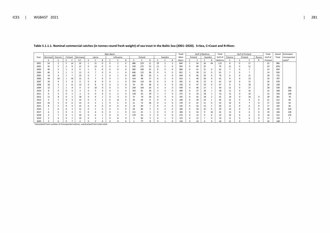
ICES | WGBAST 2021 | 281
Table 5.1.1.1. Nominal commercial catches (in tonnes round fresh weight) of sea trout in the Baltic Sea (2001–2020). S=Sea, C=Coast and R=River.
Total Total Total GrandYear Denmark Estonia Germany Main Gulf of Estonia Russia Gulf of Total
S C S C S C S C R S C R S C R S C R Basin S C C R Bothnia C S C R Finland2001 54 2 5 14 10 1 11 0 0 2 0 486 219 11 23 2 3 844 2 54 16 44 115 8 0 17 25 9842002 35 5 2 8 12 0 13 0 0 2 0 539 272 53 11 2 0 954 0 49 25 74 11 0 11 23 10512003 40 2 1 4 9 1 5 0 0 0 0 583 169 32 8 3 0 858 0 41 21 0 62 7 0 7 14 9342004 46 3 1 5 12 0 7 0 0 1 0 606 122 36 9 3 0 851 1 39 21 0 61 7 0 7 14 9262005 14 4 1 7 14 0 7 1 0 1 0 480 86 20 5 3 0 644 0 46 24 0 70 6 0 11 18 7322006 44 10 1 10 12 0 7 0 0 1 0 414 98 17 6 2 0 623 1 40 20 0 61 9 0 13 23 7072007 26 4 2 8 9 0 8 0 0 1 0 354 133 39 6 3 0 592 0 45 15 0 61 13 0 12 26 6782008 18 4 1 11 13 0 8 0 0 2 0 34 90 48 4 3 0 236 0 47 19 0 67 8 0 18 26 3282009 12 7 1 8 4 0 10 0 0 2 0 259 103 26 3 3 0 439 0 46 17 1 64 11 0 17 28 530 2662010 8 5 0 6 3 0 5 0 0 2 0 343 81 30 2 3 0 489 0 37 20 1 58 11 0 10 22 568 2992011 6 5 0 5 3 0 0 6 0 2 0 139 65 39 1 2 0 275 0 33 18 1 53 12 0 10 22 350 1482012 11 8 0 5 18 0 4 1 0 3 0 37 74 26 0 3 0 191 0 41 18 2 61 14 0 16 0 29 281 702013 4 7 0 6 14 0 5 1 0 11 0 43 44 8 0 3 0 148 0 29 14 1 44 12 0 9 0 21 212 602014 10 5 0 6 14 0 5 1 0 5 0 21 72 28 0 3 0 170 0 22 11 0 33 10 0 7 0 17 220 542015 8 5 0 4 14 0 4 0 0 6 0 13 83 7 0 2 0 145 0 16 13 1 30 11 0 6 0 17 192 662016 1 6 0 3 12 0 5 0 0 4 0 62 86 3 0 2 0 184 0 18 10 0 29 14 0 6 0 20 232 1042017 6 5 0 3 9 0 4 0 0 1 0 111 41 1 0 3 0 184 0 16 9 16 41 13 0 6 0 19 244 1282018 3 7 0 1 10 0 6 1 0 0 7 179 55 3 0 2 0 274 0 13 9 0 22 10 0 6 0 16 312 1702019 3 6 0 2 10 0 4 1 0 8 0 3 82 3 0 1 0 123 0 12 7 0 19 11 0 6 0 17 159 22020 2 6 0 7 2 0 5 0 0 0 6 1 77 8 0 1 0 116 0 10 6 0 16 11 0 5 0 16 148 1
*calculated from number of misreported salmon, substracted from total catch.
Estimated misreported catch*
Finland Latvia Lithuania Poland Sweden Finland Sweden FinlandMain Basin Gulf of Bothnia Gulf of Finland
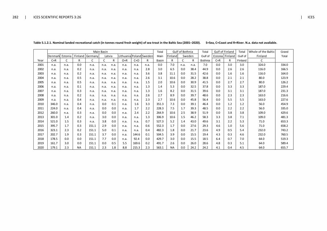
282 | ICES SCIENTIFIC REPORTS 3:26 | ICES
Table 5.1.2.1. Nominal landed recreational catch (in tonnes round fresh weight) of sea trout in the Baltic Sea (2001–2020). S=Sea, C=Coast and R=River. N.a. data not available.
Total Total Total Whole of the Baltic GrandDenmark Estonia Finland Germany Lithuania Poland Sweden Main Finland Gulf of Estonia Finland Gulf of Finland Total
Year C+R C R C C R O+R C+O R Basin R C R Bothnia C+R R Finland C2001 n.a. n.a. 0.0 n.a. n.a. n.a. n.a. n.a. n.a. 0.0 7.0 n.a. n.a. 7.0 0.0 3.0 3.0 324.0 334.02002 n.a. n.a. 0.2 n.a. n.a. n.a. n.a. n.a. 2.8 3.0 6.5 0.0 38.4 44.9 0.0 2.6 2.6 116.0 166.52003 n.a. n.a. 0.2 n.a. n.a. n.a. n.a. n.a. 3.6 3.8 11.1 0.0 31.5 42.6 0.0 1.6 1.6 116.0 164.02004 n.a. n.a. 0.5 n.a. n.a. n.a. n.a. n.a. 2.6 3.1 10.6 0.0 28.2 38.8 0.0 2.1 2.1 80.0 123.92005 n.a. n.a. 0.5 n.a. n.a. n.a. n.a. n.a. 1.5 2.0 10.6 0.0 30.9 41.5 0.0 2.7 2.7 80.0 126.22006 n.a. n.a. 0.1 n.a. n.a. n.a. n.a. n.a. 1.3 1.4 5.3 0.0 32.5 37.8 0.0 3.3 3.3 187.0 229.42007 n.a. n.a. 0.3 n.a. n.a. n.a. n.a. n.a. 1.3 1.6 8.2 0.0 31.5 39.6 0.0 3.1 3.1 187.0 231.32008 n.a. n.a. 0.2 n.a. n.a. n.a. n.a. n.a. 2.6 2.7 8.9 0.0 39.7 48.6 0.0 2.3 2.3 163.0 216.62009 n.a. n.a. 0.4 n.a. n.a. n.a. n.a. n.a. 2.3 2.7 10.6 0.0 45.8 56.4 0.0 5.5 5.5 163.0 227.62010 346.0 n.a. 0.4 n.a. 0.0 0.1 n.a. 1.6 3.3 351.3 7.3 0.0 39.1 46.4 0.0 1.2 1.2 56.0 454.92011 224.0 n.a. 0.4 n.a. 0.0 0.0 n.a. 1.7 2.2 228.3 7.5 1.7 39.3 48.5 0.0 2.2 2.2 56.0 335.02012 260.0 n.a. 0.3 n.a. 0.0 0.0 n.a. 2.4 2.2 264.9 10.6 2.5 38.9 51.9 0.0 3.8 3.8 109.0 429.62013 301.0 1.4 0.2 n.a. 3.0 0.0 n.a. n.a. 1.3 306.9 10.6 1.5 46.2 58.3 3.3 3.8 7.1 109.0 481.32014 521.0 1.5 0.3 n.a. 3.8 0.0 n.a. n.a. 0.7 527.3 5.2 1.4 43.0 49.6 3.1 2.2 5.3 71.0 653.32015 395.7 1.7 0.3 151.1 2.9 0.0 n.a. n.a. 0.6 552.3 1.7 0.0 27.6 29.3 4.6 1.0 5.6 71.0 658.22016 323.1 2.3 0.2 151.1 5.0 0.1 n.a. n.a. 0.4 482.3 1.8 0.0 21.7 23.6 4.9 0.5 5.4 232.0 743.22017 202.7 1.9 0.3 151.1 3.7 0.0 n.a. 144.6 0.1 504.5 3.9 0.0 15.5 19.4 4.3 0.3 4.6 232.0 760.52018 178.5 0.0 0.0 151.1 7.7 0.0 n.a. 92.4 0.0 429.7 3.0 0.0 15.5 18.5 6.4 0.7 7.0 64.0 519.32019 161.7 3.0 0.0 151.1 0.0 0.5 5.5 169.6 0.2 491.7 2.6 0.0 26.0 28.6 4.8 0.3 5.1 64.0 589.42020 179.1 2.3 NA 151.1 2.3 1.8 8.8 215.3 2.3 563.1 NA 0.0 24.2 24.2 4.1 0.4 4.5 64.0 655.7
Main BasinLatvia Sweden
Gulf of Finland Gulf of Bothnia
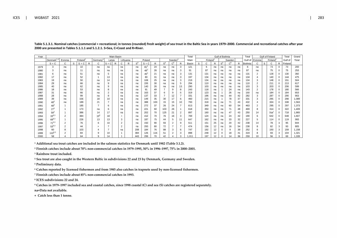
ICES | WGBAST 2021 | 283
Table 5.1.3.1. Nominal catches (commercial + recreational; in tonnes (rounded) fresh weight) of sea trout in the Baltic Sea in years 1979–2000. Commercial and recreational catches after year 2000 are presented in Tables 5.1.1.1 and 5.1.2.1. S=Sea, C=Coast and R=River.
1 Additional sea trout catches are included in the salmon statistics for Denmark until 1982 (Table 3.1.2). 2 Finnish catches include about 70% non-commercial catches in 1979–1995, 50% in 1996–1997, 75% in 2000–2001. 3 Rainbow trout included. 4 Sea trout are also caught in the Western Baltic in subdivisions 22 and 23 by Denmark, Germany and Sweden. 5 Preliminary data. 6 Catches reported by licensed fishermen and from 1985 also catches in trapnets used by non-licensed fishermen. 7 Finnish catches include about 85% non-commercial catches in 1993. 8 ICES subdivisions 22 and 24. 9 Catches in 1979–1997 included sea and coastal catches, since 1998 coastal (C) and sea (S) catches are registered separately. na=Data not available. + Catch less than 1 tonne.
Year Total Total Total GrandDenmark1,4 Estonia Germany4 Main Finland2 Sweden Gulf of Estonia Gulf of Total
S + C C S S + C R C S + C R C R S9 S + C R S6 C6 R Basin S C R S6 C6 R Bothnia C S C R Finland1979 3 na 10 na na na na 813 24 na na 3 121 6 na na na na 6 na 73 0 73 2001980 3 na 11 na na na na 483 26 na na 3 91 87 na na na na 87 na 75 0 75 2531981 6 na 51 na 5 na na 453 21 na na 3 131 131 na na na na 131 2 128 0 130 3921982 17 na 52 1 13 na na 80 31 na na 3 197 134 na na na na 134 4 140 0 144 4751983 19 na 50 na 14 na na 108 25 na na 3 219 134 na na na na 134 3 148 0 151 5041984 29 na 66 na 9 na na 155 30 na na 5 294 110 na na na na 110 2 211 0 213 6171985 40 na 62 na 9 na na 140 26 na na 13 290 103 na na na na 103 3 203 0 206 5991986 18 na 53 na 8 na na 91 49 7 9 8 243 118 na 1 24 na 143 2 178 0 180 5661987 31 na 66 na 2 na na 163 37 6 9 5 319 123 na 1 26 na 150 na 184 0 184 6531988 28 na 99 na 8 na na 137 33 7 12 7 331 196 na na 44 42 282 3 287 0 290 9031989 39 na 156 18 10 na na 149 35 30 17 6 460 215 na 1 78 37 331 3 295 0 298 1,0891990 483 na 189 21 7 na na 388 100 15 15 10 793 318 na na 71 43 432 4 334 0 338 1,5631991 483 1 185 7 6 na na 272 37 26 24 7 613 349 na na 60 54 463 2 295 0 297 1,3731992 273 1 173 na 6 na na 221 60 103 26 1 618 350 na na 71 48 469 8 314 0 322 1,4091993 593 1 386 14 17 na na 202 70 125 21 2 897 160 na na 47 43 250 14 7047 0 718 1,8651994 338,3 2 384 158 18 + na 152 70 76 16 3 769 124 na na 24 42 190 6 642 0 648 1,6071995 698,3 1 226 13 13 3 na 187 75 44 5 11 647 162 na na 33 32 227 5 114 0 119 9931996 718,3 2 76 6 10 2 na 150 90 93 2 9 511 151 25 na 20 42 238 14 78 3 95 8441997 538,3 2 44 + 7 2 na 200 80 72 7 7 474 156 12 na 16 54 238 8 82 3 93 8051998 60 8 103 4 7 na 208 184 76 88 3 6 747 192 12 0 9 39 252 6 150 3 159 1,1581999 1108,3 2 84 9 10 1 384 126 116 51 2 3 898 248 12 0 18 41 319 8 93 3 104 1,3212000 58 4 64 9 14 1 443 299 70 42 4 3 1,011 197 12 0 14 36 259 10 56 3 69 1,339
Main Basin Gulf of Bothnia Gulf of FinlandFinland2 Latvia Lithuania Finland2 Sweden4Poland
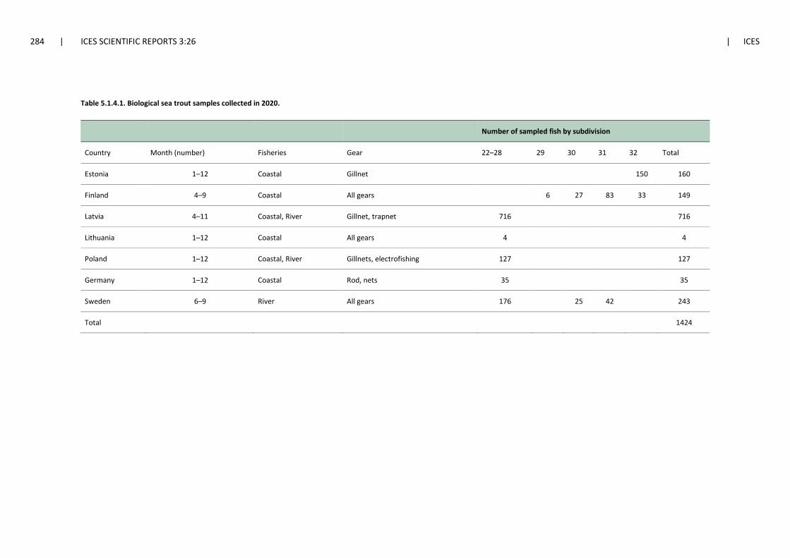
284 | ICES SCIENTIFIC REPORTS 3:26 | ICES
Table 5.1.4.1. Biological sea trout samples collected in 2020.
Number of sampled fish by subdivision
Country Month (number) Fisheries Gear 22–28 29 30 31 32 Total
Estonia 1–12 Coastal Gillnet 150 160
Finland 4–9 Coastal All gears 6 27 83 33 149
Latvia 4–11 Coastal, River Gillnet, trapnet 716 716
Lithuania 1–12 Coastal All gears 4 4
Poland 1–12 Coastal, River Gillnets, electrofishing 127 127
Germany 1–12 Coastal Rod, nets 35 35
Sweden 6–9 River All gears 176 25 42 243
Total 1424
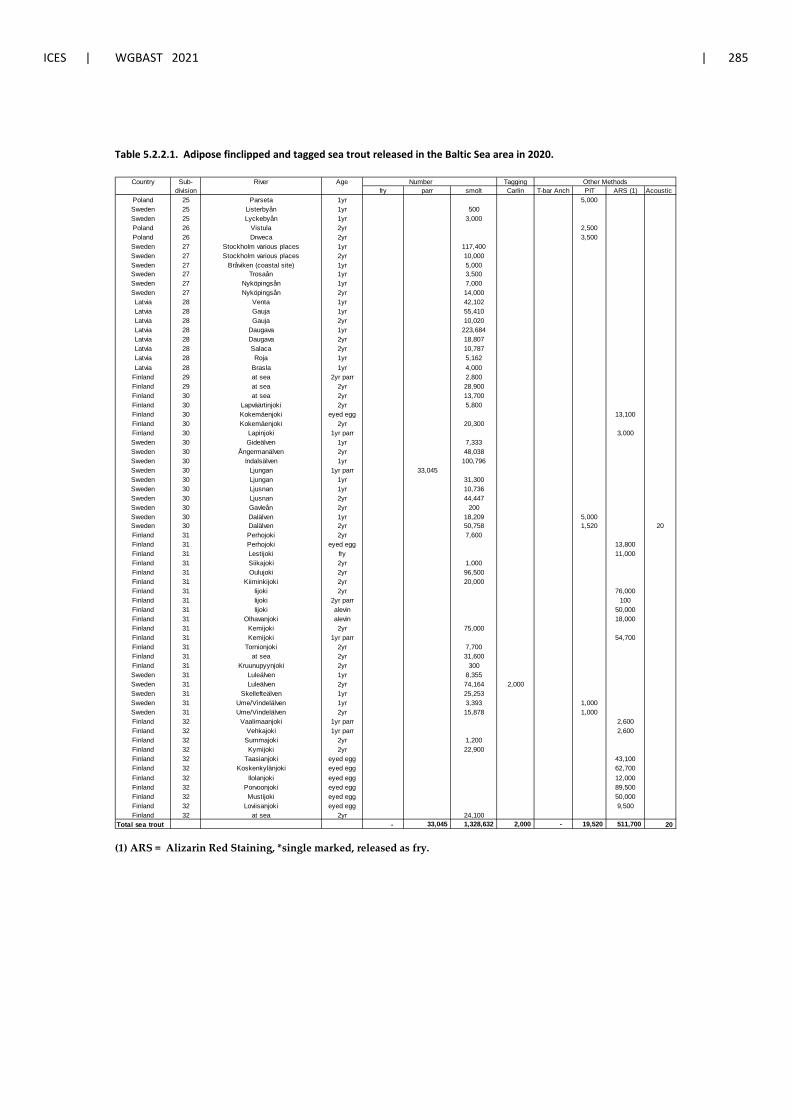
ICES | WGBAST 2021 | 285
Table 5.2.2.1. Adipose finclipped and tagged sea trout released in the Baltic Sea area in 2020.
(1) ARS = Alizarin Red Staining, *single marked, released as fry.
Country Sub- River Age Taggingdivision fry parr smolt Carlin T-bar Anch PIT ARS (1) Acoustic
Poland 25 Parseta 1yr 5,000Sweden 25 Listerbyån 1yr 500Sweden 25 Lyckebyån 1yr 3,000Poland 26 Vistula 2yr 2,500Poland 26 Drweca 2yr 3,500Sweden 27 Stockholm various places 1yr 117,400Sweden 27 Stockholm various places 2yr 10,000Sweden 27 Bråviken (coastal site) 1yr 5,000Sweden 27 Trosaån 1yr 3,500Sweden 27 Nyköpingsån 1yr 7,000Sweden 27 Nyköpingsån 2yr 14,000Latvia 28 Venta 1yr 42,102Latvia 28 Gauja 1yr 55,410Latvia 28 Gauja 2yr 10,020Latvia 28 Daugava 1yr 223,684Latvia 28 Daugava 2yr 18,807Latvia 28 Salaca 2yr 10,787Latvia 28 Roja 1yr 5,162Latvia 28 Brasla 1yr 4,000
Finland 29 at sea 2yr parr 2,800Finland 29 at sea 2yr 28,900Finland 30 at sea 2yr 13,700Finland 30 Lapväärtinjoki 2yr 5,800Finland 30 Kokemäenjoki eyed egg 13,100Finland 30 Kokemäenjoki 2yr 20,300Finland 30 Lapinjoki 1yr parr 3,000Sweden 30 Gideälven 1yr 7,333Sweden 30 Ångermanälven 2yr 48,038Sweden 30 Indalsälven 1yr 100,796Sweden 30 Ljungan 1yr parr 33,045Sweden 30 Ljungan 1yr 31,300Sweden 30 Ljusnan 1yr 10,736Sweden 30 Ljusnan 2yr 44,447Sweden 30 Gavleån 2yr 200Sweden 30 Dalälven 1yr 18,209 5,000Sweden 30 Dalälven 2yr 50,758 1,520 20Finland 31 Perhojoki 2yr 7,600Finland 31 Perhojoki eyed egg 13,800Finland 31 Lestijoki fry 11,000Finland 31 Siikajoki 2yr 1,000Finland 31 Oulujoki 2yr 96,500Finland 31 Kiiminkijoki 2yr 20,000Finland 31 Iijoki 2yr 76,000Finland 31 Iijoki 2yr parr 100Finland 31 Iijoki alevin 50,000Finland 31 Olhavanjoki alevin 18,000Finland 31 Kemijoki 2yr 75,000Finland 31 Kemijoki 1yr parr 54,700Finland 31 Tornionjoki 2yr 7,700Finland 31 at sea 2yr 31,600Finland 31 Kruunupyynjoki 2yr 300Sweden 31 Luleälven 1yr 8,355Sweden 31 Luleälven 2yr 74,164 2,000Sweden 31 Skellefteälven 1yr 25,253Sweden 31 Ume/Vindelälven 1yr 3,393 1,000Sweden 31 Ume/Vindelälven 2yr 15,878 1,000Finland 32 Vaalimaanjoki 1yr parr 2,600Finland 32 Vehkajoki 1yr parr 2,600Finland 32 Summajoki 2yr 1,200Finland 32 Kymijoki 2yr 22,900Finland 32 Taasianjoki eyed egg 43,100Finland 32 Koskenkylänjoki eyed egg 62,700Finland 32 Ilolanjoki eyed egg 12,000Finland 32 Porvoonjoki eyed egg 89,500Finland 32 Mustijoki eyed egg 50,000Finland 32 Loviisanjoki eyed egg 9,500Finland 32 at sea 2yr 24,100
Total sea trout - 33,045 1,328,632 2,000 - 19,520 511,700 20
Other Methods Number
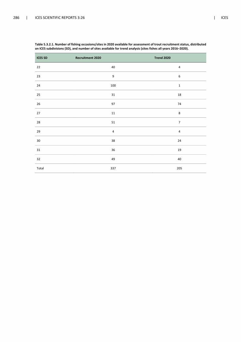
286 | ICES SCIENTIFIC REPORTS 3:26 | ICES
Table 5.3.2.1. Number of fishing occasions/sites in 2020 available for assessment of trout recruitment status, distributed on ICES subdivisions (SD), and number of sites available for trend analysis (sites fishes all years 2016–2020).
ICES SD Recruitment 2020 Trend 2020
22 40 4
23 9 6
24 100 1
25 31 18
26 97 74
27 11 8
28 51 7
29 4 4
30 38 24
31 36 19
32 49 40
Total 337 205
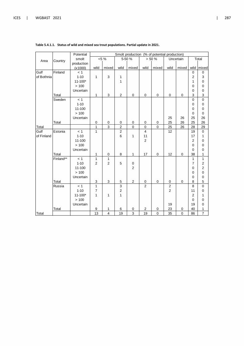
ICES | WGBAST 2021 | 287
Table 5.4.1.1. Status of wild and mixed sea trout populations. Partial update in 2021.
wild mixed wild mixed wild mixed wild mixed wild mixedGulf Finland < 1 0 0of Bothnia 1-10 1 3 1 2 3
11-100* 1 1 0> 100 0 0
Uncertain 0 0Total 1 3 2 0 0 0 0 0 3 3Sweden < 1 0 0
1-10 0 011-100 0 0> 100 0 0
Uncertain 25 26 25 26Total 0 0 0 0 0 0 25 26 25 26
Total 1 3 2 0 0 0 25 26 28 29Gulf Estonia < 1 1 2 4 12 19 0of Finland 1-10 6 1 11 17 1
11-100 2 2 0> 100 0 0
Uncertain 0 0Total 1 0 8 1 17 0 12 0 38 1Finland** < 1 1 1 1 1
1-10 2 2 5 0 7 211-100 2 0 2> 100 0 0
Uncertain 0 0Total 3 3 5 2 0 0 0 0 8 5Russia < 1 1 3 2 2 8 0
1-10 7 2 2 11 011-100* 1 1 1 2 1> 100 0 0
Uncertain 19 19 0Total 9 1 6 0 2 0 23 0 40 1
Total 13 4 19 3 19 0 35 0 86 7
Area Country <5 % TotalUncertain> 50 %5-50 %Smolt production (% of potential production)Potential
smolt production
(x1000)
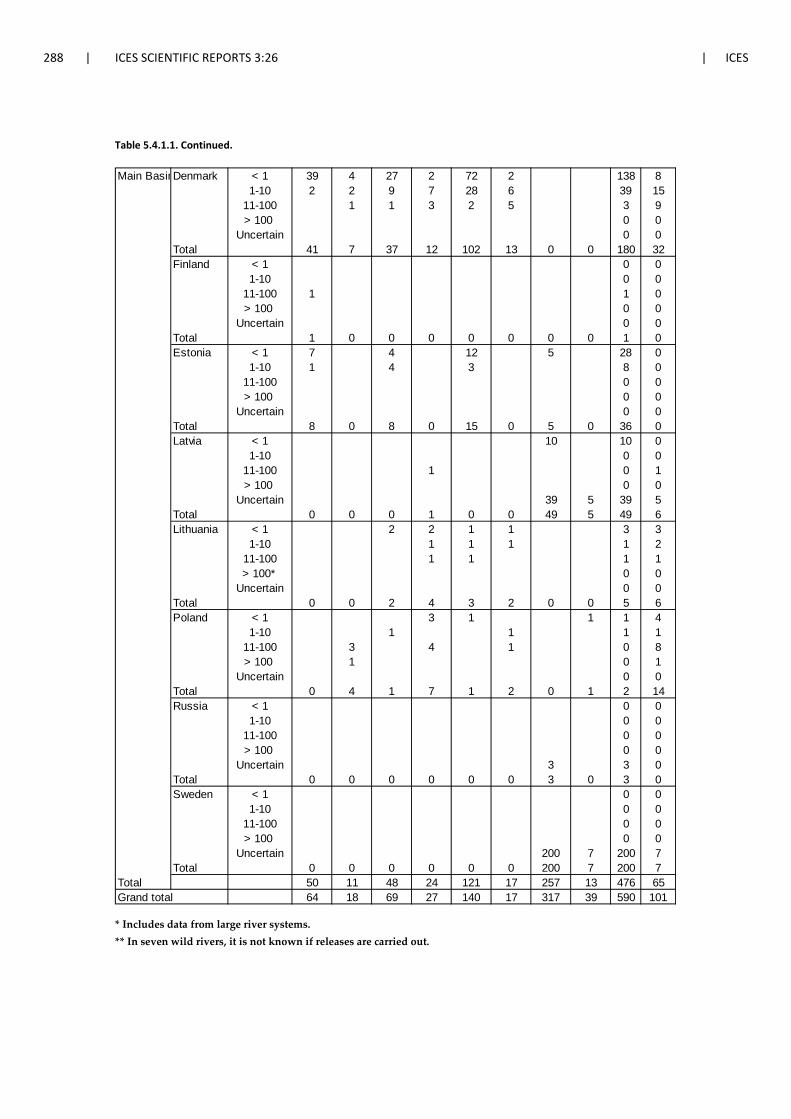
288 | ICES SCIENTIFIC REPORTS 3:26 | ICES
Table 5.4.1.1. Continued.
* Includes data from large river systems. ** In seven wild rivers, it is not known if releases are carried out.
Main BasinDenmark < 1 39 4 27 2 72 2 138 81-10 2 2 9 7 28 6 39 15
11-100 1 1 3 2 5 3 9> 100 0 0
Uncertain 0 0Total 41 7 37 12 102 13 0 0 180 32Finland < 1 0 0
1-10 0 011-100 1 1 0> 100 0 0
Uncertain 0 0Total 1 0 0 0 0 0 0 0 1 0Estonia < 1 7 4 12 5 28 0
1-10 1 4 3 8 011-100 0 0> 100 0 0
Uncertain 0 0Total 8 0 8 0 15 0 5 0 36 0Latvia < 1 10 10 0
1-10 0 011-100 1 0 1> 100 0 0
Uncertain 39 5 39 5Total 0 0 0 1 0 0 49 5 49 6Lithuania < 1 2 2 1 1 3 3
1-10 1 1 1 1 211-100 1 1 1 1> 100* 0 0
Uncertain 0 0Total 0 0 2 4 3 2 0 0 5 6Poland < 1 3 1 1 1 4
1-10 1 1 1 111-100 3 4 1 0 8> 100 1 0 1
Uncertain 0 0Total 0 4 1 7 1 2 0 1 2 14Russia < 1 0 0
1-10 0 011-100 0 0> 100 0 0
Uncertain 3 3 0Total 0 0 0 0 0 0 3 0 3 0Sweden < 1 0 0
1-10 0 011-100 0 0> 100 0 0
Uncertain 200 7 200 7Total 0 0 0 0 0 0 200 7 200 7
Total 50 11 48 24 121 17 257 13 476 65Grand total 64 18 69 27 140 17 317 39 590 101
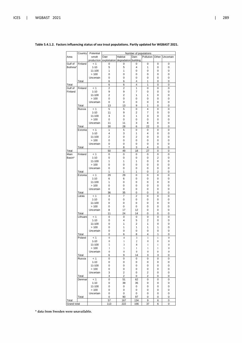
ICES | WGBAST 2021 | 289
Table 5.4.1.2. Factors influencing status of sea trout populations. Partly updated for WGBAST 2021.
* data from Sweden were unavailable.
Area
Gulf of Finland < 1 0 0 0 0 0 0Bothnia* 1-10 5 5 4 1 0 0
11-100 1 1 0 0 0 0> 100 0 0 0 0 0 0
Uncertain 0 0 0 0 0 0Total 6 6 4 1 0 0
Total 6 6 4 1 0 0Gulf of Finland < 1 2 2 1 0 0 0Finland 1-10 9 9 7 0 0 0
11-100 2 2 1 1 0 0> 100 0 0 0 0 0 0
Uncertain 0 0 0 0 0 0Total 13 13 9 1 0 0Russia < 1 5 5 0 4 0 0
1-10 11 9 2 7 0 011-100 3 3 1 3 0 0> 100 0 0 0 0 0 0
Uncertain 11 11 3 8 0 0Total 30 28 6 22 0 0Estonia < 1 1 5 0 0 0 0
1-10 4 3 1 4 0 011-100 2 0 2 0 0 0> 100 0 0 0 0 0 0
Uncertain 0 0 0 0 0 0Total 7 8 3 4 0 0
Total 50 49 18 27 0 0Main Finland < 1 0 0 0 0 0 0Basin* 1-10 0 0 0 0 2 0
11-100 1 1 1 0 0 0> 100 0 0 0 0 0 0
Uncertain 0 0 0 0 0 0Total 1 1 1 0 2 0Estonia < 1 29 29 0 0 0 0
1-10 6 6 0 0 0 011-100 1 0 0 0 0 0> 100 0 0 0 0 0 0
Uncertain 0 0 0 0 0 0Total 36 35 0 0 0 0Latvia < 1 3 7 2 0 0 0
1-10 0 0 0 0 0 011-100 0 0 0 0 0 0> 100 0 0 0 0 0 0
Uncertain 8 17 12 0 0 0Total 11 24 14 0 0 0Lithuania < 1 0 0 0 0 0 0
1-10 0 4 5 2 0 011-100 0 1 2 1 0 0> 100 0 1 1 1 1 0
Uncertain 0 0 0 0 0 0Total 0 6 8 4 1 0Poland < 1 0 4 3 1 1 0
1-10 0 1 2 0 0 011-100 5 3 8 1 1 0> 100 1 1 1 1 1 0
Uncertain 0 0 0 0 0 0Total 6 9 14 3 3 0Russia < 1 0 0 0 0 0 0
1-10 0 0 0 0 0 011-100 0 0 0 0 0 0> 100 0 0 0 0 0 0
Uncertain 3 2 0 2 0 0Total 3 2 0 2 0 0Denmark < 1 0 51 62 0 0 0
1-10 0 39 35 0 0 011-100 0 0 0 0 0 0> 100 0 0 0 0 0 0
Uncertain 0 0 0 0 0 0Total 0 90 97 0 0 0
Total 57 167 134 9 6 0Grand total 113 222 156 37 6 0
Country Potential smolt
production Over exploitation
Habitat degradation
Number of populations Pollution Other UncertainDam
building
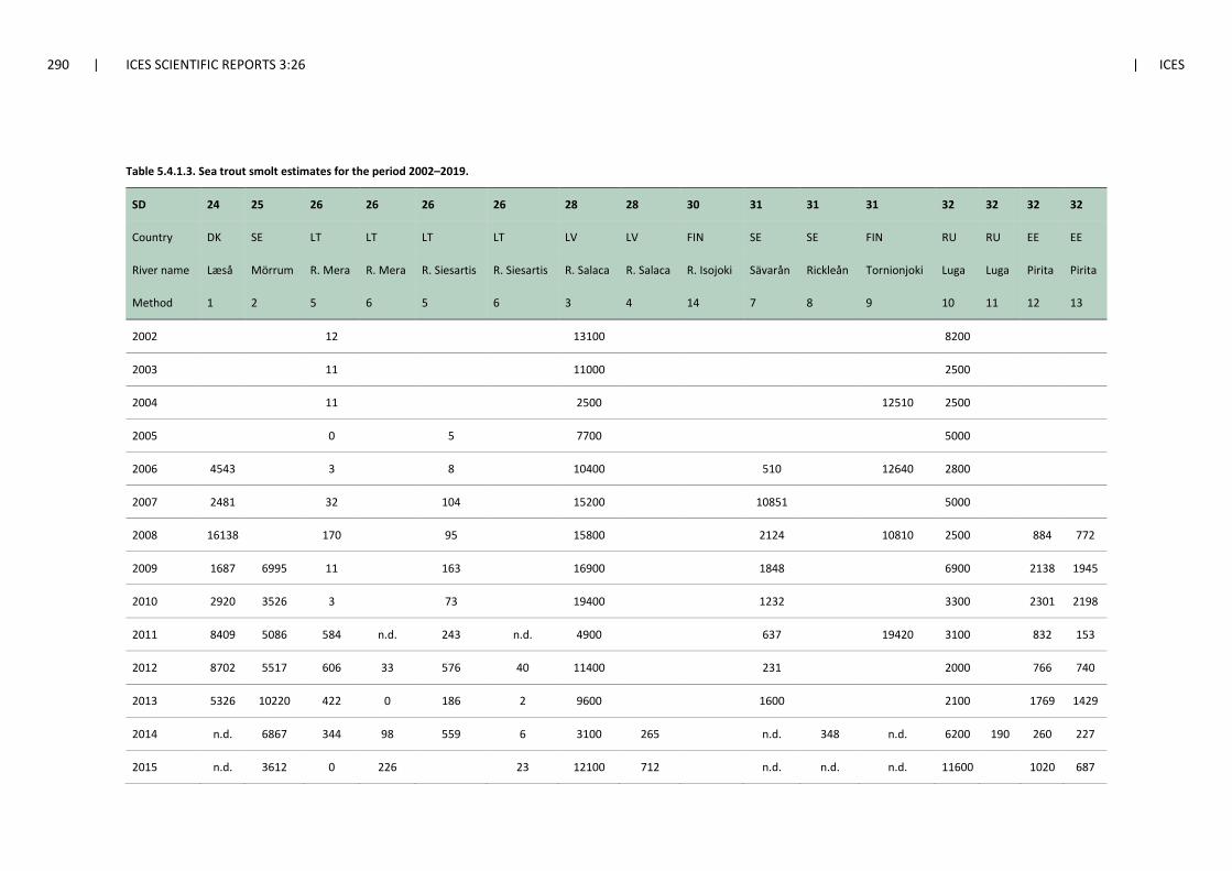
290 | ICES SCIENTIFIC REPORTS 3:26 | ICES
Table 5.4.1.3. Sea trout smolt estimates for the period 2002–2019.
SD 24 25 26 26 26 26 28 28 30 31 31 31 32 32 32 32
Country DK SE LT LT LT LT LV LV FIN SE SE FIN RU RU EE EE
River name Læså Mörrum R. Mera R. Mera R. Siesartis R. Siesartis R. Salaca R. Salaca R. Isojoki Sävarån Rickleån Tornionjoki Luga Luga Pirita Pirita
Method 1 2 5 6 5 6 3 4 14 7 8 9 10 11 12 13
2002
12
13100
8200
2003
11
11000
2500
2004
11
2500
12510 2500
2005
0
5
7700
5000
2006 4543
3
8
10400
510
12640 2800
2007 2481
32
104
15200
10851
5000
2008 16138
170
95
15800
2124
10810 2500
884 772
2009 1687 6995 11
163
16900
1848
6900
2138 1945
2010 2920 3526 3
73
19400
1232
3300
2301 2198
2011 8409 5086 584 n.d. 243 n.d. 4900
637
19420 3100
832 153
2012 8702 5517 606 33 576 40 11400
231
2000
766 740
2013 5326 10220 422 0 186 2 9600
1600
2100
1769 1429
2014 n.d. 6867 344 98 559 6 3100 265 n.d. 348 n.d. 6200 190 260 227
2015 n.d. 3612 0 226
23 12100 712 n.d. n.d. n.d. 11600
1020 687
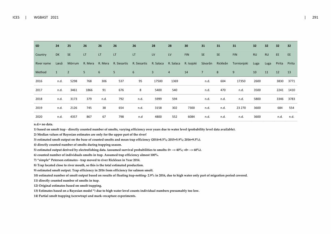
ICES | WGBAST 2021 | 291
SD 24 25 26 26 26 26 28 28 30 31 31 31 32 32 32 32
Country DK SE LT LT LT LT LV LV FIN SE SE FIN RU RU EE EE
River name Læså Mörrum R. Mera R. Mera R. Siesartis R. Siesartis R. Salaca R. Salaca R. Isojoki Sävarån Rickleån Tornionjoki Luga Luga Pirita Pirita
Method 1 2 5 6 5 6 3 4 14 7 8 9 10 11 12 13
2016 n.d. 5298 768 306 537 95 17500 1369 n.d. 604 17350 2600
3830 3771
2017 n.d. 3461 1866 91 676 8 5400 540 n.d. 470 n.d. 3500
2241 1410
2018 n.d. 3173 379 n.d. 792 n.d. 5999 594 n.d. n.d. n.d. 5800 3346 3783
2019 n.d. 2126 745 38 654 n.d. 3158 302 7300 n.d. n.d. 23 270 3600
684 554
2020 n.d. 4357 867 67 798 n.d 4800 552 6084 n.d. n.d. n.d. 3600 n.d. n.d.
n.d.= no data. 1) based on smolt trap - directly counted number of smolts, varying efficiency over years due to water level (probability level data available). 2) Median values of Bayesian estimates are only for the upper part of the river! 3) estimated smolt output on the base of counted smolts and mean trap efficiency (2014=8.5%; 2015=5.9%; 2016=9.5%). 4) directly counted number of smolts during trapping season. 5) estimated output derived by electrofishing data. (assumed survival probabilities to smolts: 0+ --> 40%; >0+ --> 60%). 6) counted number of individuals smolts in trap. Assumed trap efficiency almost 100%. 7) “simple” Peterson estimates - trap moved to river Ricklean in Year 2014. 8) Trap located close to river mouth, so this is the total estimated production. 9) estimated smolt output. Trap efficiency in 2016 from efficiency for salmon smolt. 10) estimated number of smolt output based on results of floating trap-netting- 2.9% in 2016, due to high water only part of migration period covered. 11) directly counted number of smolts in trap. 12) Original estimates based on smolt trapping. 13) Estimates based on a Bayesian model *) due to high water level counts individual numbers presumably too low. 14) Partial smolt trapping (screwtrap) and mark–recapture experiments.
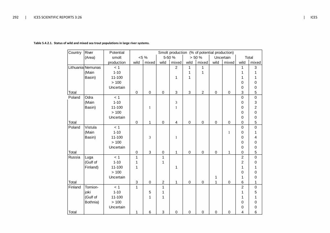
292 | ICES SCIENTIFIC REPORTS 3:26 | ICES
Table 5.4.2.1. Status of wild and mixed sea trout populations in large river systems.
River(Area)
wild mixed wild mixed wild mixed wild mixed wild mixedLithuania Nemunas < 1 2 1 1 1 3
(Main 1-10 1 1 1 1Basin) 11-100 1 1 1 1
> 100 0 0Uncertain 0 0
Total 0 0 0 3 3 2 0 0 3 5Poland Odra < 1 0 0
(Main 1-10 3 0 3Basin) 11-100 1 1 0 2
> 100 0 0Uncertain 0 0
Total 0 1 0 4 0 0 0 0 0 5Poland Vistula < 1 0 0
(Main 1-10 1 0 1Basin) 11-100 3 1 0 4
> 100 0 0Uncertain 0 0
Total 0 3 0 1 0 0 0 1 0 5Russia Luga < 1 1 1 2 0
(Gulf of 1-10 1 1 2 0Finland) 11-100 1 1 1 1
> 100 0 0Uncertain 1 1 0
Total 3 0 2 1 0 0 1 0 6 1Finland Tornion- < 1 1 1 2 0
joki 1-10 5 1 1 5(Gulf of 11-100 1 1 1 1Bothnia) > 100 0 0
Uncertain 0 0Total 1 6 3 0 0 0 0 0 4 6
Country<5 % TotalUncertain> 50 %5-50 %
Smolt production (% of potential production)Potential smolt
production

ICES | WGBAST 2021 | 293
Table 5.6.1. Sea trout smolt releases (x1000) into the Baltic Sea by country and subdivision in 1988–2019. Note that project based fisheries enhancement releases included.
country age 1988 1989 1990 1991 1992 1993 1994 1995 1996 1997 1998 1999 2000 2001 2002 2003 2004 2005 2006 2007 2008 2009 2010 2011 2012 2013 2014 2015 2016 2017 2018 2019 2020DK 1yr 5 1 4 4 4 19 17 177 177 177 196 196 19 751 634 614 562 562 398 387 387 365 261 281 272 272 333 313 589 591 550 322 687
2yr 30 30 30 30 21 9 9 2 2 2 2 2 0 0 0 0 0 0EE 1yr 50 5 5 3
2yr 5 6 10 10 16 28 30 32 30 32 30 32 30 23 25 2 21 20 17 21 26 21 5FI 1yr 11 1 0 4 26 28 1 15 35 52 45 52 18 115 40 5 30 14 15
2yr 129 169 165 123 103 171 144 181 153 182 168 258 197 131 134 244 303 164 187 218 136 113 121 76 107 123 93 97 103 92 87 973yr 35 16 0 26 1 8 0 13 17 25 35 34 24 9 16 16 15 8 14 4 0
LT 1yr 5 5 4 4 10 23 58 45 11 10 23 29 32 32 31 11 262yr 3 1 0
LV 1yr 1 1 6 26 44 26 24 20 1 1 7 25 114 160 170 74 91 113 63 50 153 236 270 161 115 98 308 391 296 187 3412yr 1 4 6 7 5 2 11 29 2 10 67 116 177 112 132 65 8 69 13 33 29
PL 1yr 51 85 102 2 148 140 266 483 298 492 330 138 151 211 30 16 46 322 455 188 358 434 267 132 174 243 289 328 301 546 1024 431 7872yr 857 847 498 248 376 845 523 642 821 1028 1001 924 845 733 739 804 765 843 968 1261 1021 834 1060 936 981 1046 888 619 634 651 8 515 290
SE 1yr 13 9 8 19 41 18 6 4 23 19 90 7 10 108 10 116 11 131 15 76 180 129 170 118 138 207 156 183 156 144 156 1312yr 32 51 78 61 44 46 84 90 60 95 87 76 100 93 40 48 103 44 36 63 78 31 31 27 35 20 20 30 17 33 40 17 29
DE 1yr 14 14 14 13 15 14 15 14 15 15 7 10Main Basin Total 1010 1167 903 544 795 1239 1114 1600 1576 2029 1880 1730 1445 2204 1935 1925 1921 2322 2513 2406 2453 2255 2123 2052 1953 2058 2025 1779 2190 2518 2214 1766 2426
FI 1yr 9 7 1 5 33 1252yr 358 579 700 716 527 525 510 663 639 483 540 462 478 503 451 305 358 477 541 608 676 426 519 472 503 493 477 411 417 458 401 3633yr 99 30 5 18 39 15 1 28 12 49 10 34 75 28 11 15 6 27 9 27 20 4 4 8 3 1 1 1 1
SE 1yr 19 7 6 1 40 61 55 110 197 181 219 239 253 220 198 215 2052yr 445 392 406 406 413 376 460 642 554 429 407 372 405 424 380 428 361 413 569 530 410 428 400 420 395 311 293 230 190 276 295 259 236
Gulf of Bothnia Total 445 848 1042 1118 1147 942 1001 1159 1244 1087 939 923 901 982 911 890 681 776 1072 1113 1086 1184 885 1052 1071 1123 1005 947 855 913 952 875 805EE 2yr 14 6 8 9 12 10 6 6 15 13 8 5 6 3 3FI 1yr 5 22 4 5 15 12 13 5 38 4 11
2yr 191 260 249 306 312 284 342 128 228 277 386 355 372 367 290 281 190 279 247 316 291 213 239 216 242 173 132 194 178 143 73 483yr 0 24 6 1 33 92 40 7 24 18 6 16 0 0 0
RU 1yr 4 3 13 95 25 10 3 7 64 44 74 88 82 84 552yr 1 0 1 0
Gulf of Finland Total 197 261 270 330 318 287 348 177 331 331 398 380 427 373 329 291 198 301 364 352 308 222 260 292 294 253 138 285 263 227 127 48Grand Total 1455 2212 2205 1932 2272 2499 2402 3106 2997 3447 3150 3050 2726 3613 3219 3144 2893 3296 3886 3883 3890 3747 3229 3365 3315 3475 3283 2863 3330 3694 3392 2768 3279
year
Main Basin 22-29
Gulf of Finland
32
Gulf of Bothnia 30-31
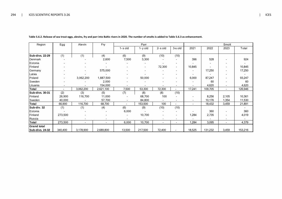
294 | ICES SCIENTIFIC REPORTS 3:26 | ICES
Table 5.6.2. Release of sea trout eggs, alevins, fry and parr into Baltic rivers in 2020. The number of smolts is added to Table 5.6.3 as enhancement.
Region Egg Alevin Fry Parr Smolt1- s old 1- y old 2- s old 3-s old 2021 2022 2023 Total
Sub-divs. 22-29 (1) (1) (4) (6) (9) (10) (10)Denmark - - 2,600 7,500 3,300 - - 396 528 - 924 Estonia - - - - - - - - - - - Finland - - - - - 72,300 - 10,845 - - 10,845 Germany - - 575,000 - - - - - 17,250 - 17,250 Latvia - - - - - - - - - - - Poland - 3,062,200 1,887,500 - 50,000 - - 6,000 87,247 - 93,247 Sweden - - 2,000 - - - - - 60 - 60 Lituania - - 154,000 - - - - - 4,620 - 4,620 Total - 3,062,200 2,621,100 7,500 53,300 72,300 - 17,241 109,705 - 126,946 Sub-divs. 30-31 (2) (3) (5) (7) (8) (8) (10)Finland 26,900 116,700 11,000 - 68,700 100 - - 8,256 2,105 10,361 Sweden 40,000 - 57,700 - 84,800 - - - 10,176 1,354 11,530 Total 66,900 116,700 68,700 - 153,500 100 - - 18,432 3,459 21,891 Sub-div. 32 (1) (1) (4) (6) (9) (10) (10) - Estonia - - - 6,000 - - - - 360 - 360 Finland 273,500 - - - 10,700 - - 1,284 2,735 - 4,019 Russia - - - - - - - - - - - Total 273,500 - - 6,000 10,700 - - 1,284 3,095 - 4,379 Grand total Sub-divs. 24-32 340,400 3,178,900 2,689,800 13,500 217,500 72,400 - 18,525 131,232 3,459 153,216
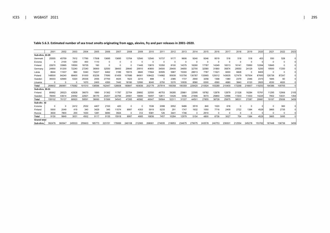
ICES | WGBAST 2021 | 295
Table 5.6.3. Estimated number of sea trout smolts originating from eggs, alevins, fry and parr releases in 2001–2020.
2001 2002 2003 2004 2005 2006 2007 2008 2009 2010 2011 2012 2013 2014 2015 2016 2017 2018 2019 2020 2021 2022 2023Sub-divs. 22-29Denmark 25555 45759 7912 17790 17508 13695 13695 13704 12540 12540 10737 9177 9606 9240 9246 9519 518 518 518 453 930 528 0Estonia 0 2100 1200 400 1110 0 0 0 0 0 0 0 0 0 0 0 0 0 0 0 0 0 0Finland 22670 33965 19550 18735 160 0 0 0 11445 13815 10350 8100 14375 16260 17787 14349 18313 16141 15990 12264 10845 0 0Germany 24900 61200 72240 27240 36900 32550 38400 29640 29910 40800 34500 29400 34650 32700 32580 31860 35874 29550 24129 5250 19500 17250 0Latvia 8644 11007 960 5340 15227 6462 3189 19015 6840 17664 30595 5987 15300 28913 7787 11621 6000 6828 0 8400 0 0 0Poland 148500 84240 68400 91000 63236 77690 61459 107686 84901 108422 114982 95939 103756 130787 133965 120012 143635 127479 167504 87693 126736 87247 0Sweden 39333 42690 5320 29335 2055 27700 4425 1623 2210 898 0 2385 1737 2940 3258 1368 1380 2379 2346 2373 1845 60 0Lituania 0 0 0 1670 2400 4350 7440 18180 12990 8040 6750 5370 10935 8580 6300 4560 4680 3840 6120 2820 4530 4620 0Total 269602 280961 175582 191510 138596 162447 128608 189847 160836 202179 207914 156358 190359 229420 210924 193289 210400 173268 216607 119253 164386 109705 0Sub-divs. 30-31Finland 80662 26523 42828 36670 1890 31362 11787 22704 29892 32550 46753 39285 25881 22595 18782 12878 12879 21328 16284 15761 11295 12906 2105Sweden 78440 43614 24092 22921 36170 20207 22756 24561 16690 16497 12811 13026 5456 21906 9073 25850 12996 17203 11003 14220 7902 13031 1354Total 159102 70137 66920 59591 38060 51569 34543 47265 46582 49047 59564 52311 31337 44501 27855 38728 25875 38531 27287 29981 19197 25936 3459Sub-div. 32Estonia 0 0 2412 2532 4407 2100 420 0 0 1536 2098 6552 9486 3519 840 1020 618 0 0 0 0 360 0Finland 5500 2049 419 340 3429 345 11574 8997 4353 5919 5233 291 1747 1632 1050 7716 2409 2722 1384 4529 3865 2735 0Russia 3630 7800 200 1630 1281 6690 3924 0 312 9381 126 3441 1746 3 2910 0 0 0 0 0 0 0 0Total 9130 9849 3031 4502 9117 9135 15918 8997 4665 16836 7457 10284 12979 5154 4800 8736 3027 754 1384 4529 3865 3095 0Grand total Sub-divs. 392476 360947 245533 255603 185773 223151 179069 246108 212083 268061 274935 218953 234675 279075 243578 240753 239301 212554 245278 153762 187448 138736 3459
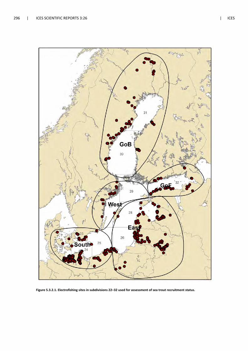
296 | ICES SCIENTIFIC REPORTS 3:26 | ICES
Figure 5.3.2.1. Electrofishing sites in subdivisions 22–32 used for assessment of sea trout recruitment status.
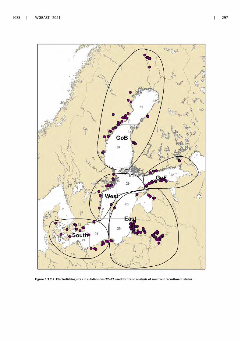
ICES | WGBAST 2021 | 297
Figure 5.3.2.2. Electrofishing sites in subdivisions 22–32 used for trend analysis of sea trout recruitment status.
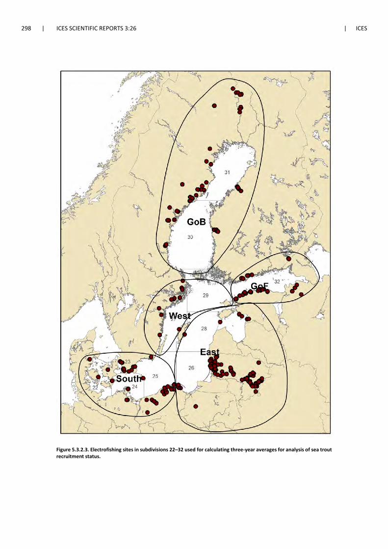
298 | ICES SCIENTIFIC REPORTS 3:26 | ICES
Figure 5.3.2.3. Electrofishing sites in subdivisions 22–32 used for calculating three-year averages for analysis of sea trout recruitment status.
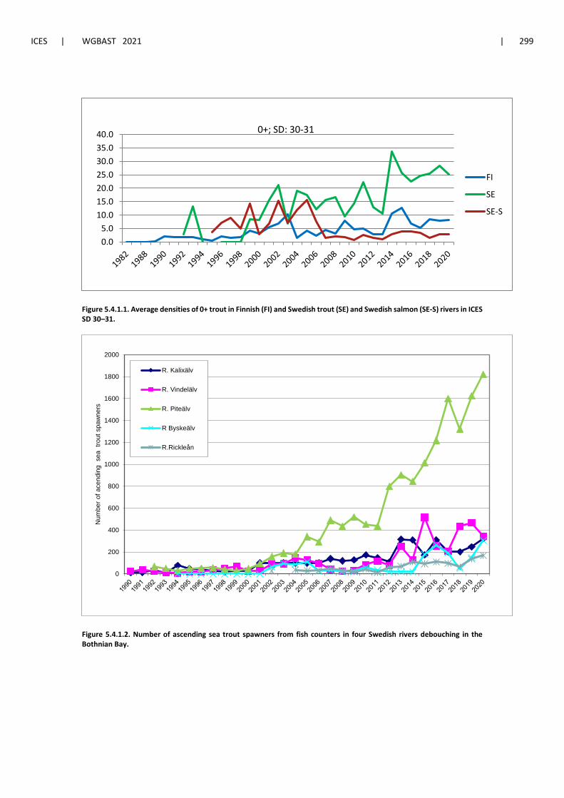
ICES | WGBAST 2021 | 299
Figure 5.4.1.1. Average densities of 0+ trout in Finnish (FI) and Swedish trout (SE) and Swedish salmon (SE-S) rivers in ICES SD 30–31.
Figure 5.4.1.2. Number of ascending sea trout spawners from fish counters in four Swedish rivers debouching in the Bothnian Bay.
0.05.0
10.015.020.025.030.035.040.0
FI
SE
SE-S
0+; SD: 30-31
0
200
400
600
800
1000
1200
1400
1600
1800
2000
Num
ber o
f ace
ndin
g s
ea t
rout
spa
wne
rs
R. Kalixälv
R. Vindelälv
R. Piteälv
R Byskeälv
R.Rickleån
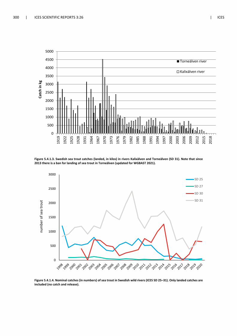
300 | ICES SCIENTIFIC REPORTS 3:26 | ICES
Figure 5.4.1.3. Swedish sea trout catches (landed, in kilos) in rivers Kalixälven and Torneälven (SD 31). Note that since 2013 there is a ban for landing of sea trout in Torneälven (updated for WGBAST 2021).
Figure 5.4.1.4. Nominal catches (in numbers) of sea trout in Swedish wild rivers (ICES SD 25–31). Only landed catches are included (no catch and release).
0
500
1000
1500
2000
2500
3000
3500
4000
4500
5000
1919
1922
1925
1928
1931
1964
1967
1970
1973
1976
1979
1982
1985
1988
1991
1994
1997
2000
2003
2006
2009
2012
2015
2018
Catc
h in
kg
Torneälven river
Kalixälven river
0
500
1000
1500
2000
2500
3000
num
ber o
f sea
trou
t
SD 25
SD 27
SD 30
SD 31
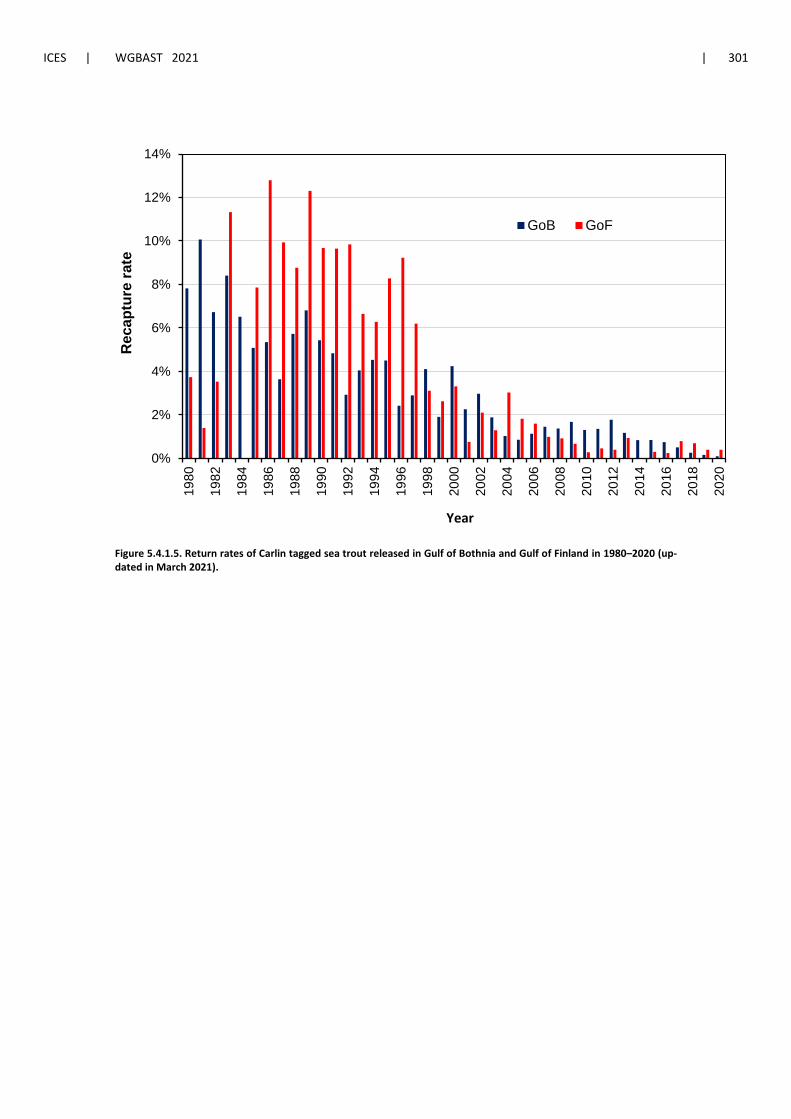
ICES | WGBAST 2021 | 301
Figure 5.4.1.5. Return rates of Carlin tagged sea trout released in Gulf of Bothnia and Gulf of Finland in 1980–2020 (up-dated in March 2021).
0%
2%
4%
6%
8%
10%
12%
14%
1980
1982
1984
1986
1988
1990
1992
1994
1996
1998
2000
2002
2004
2006
2008
2010
2012
2014
2016
2018
2020
Rec
aptu
re ra
te
Year
GoB GoF
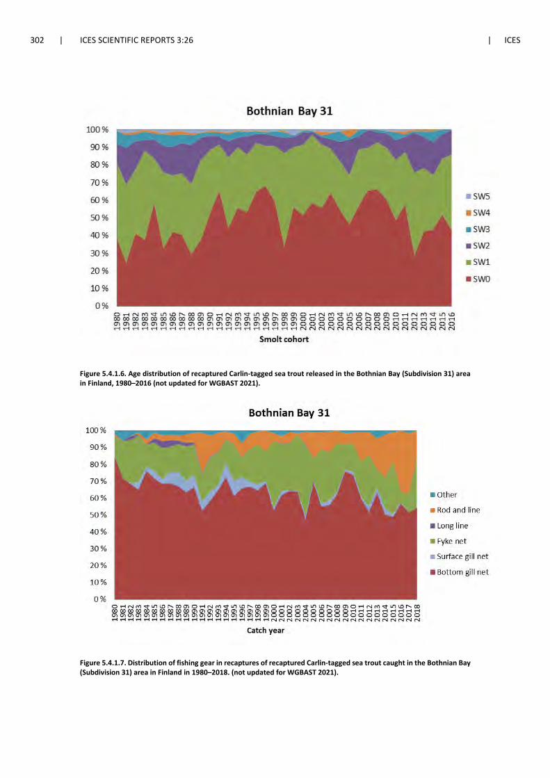
302 | ICES SCIENTIFIC REPORTS 3:26 | ICES
Figure 5.4.1.6. Age distribution of recaptured Carlin-tagged sea trout released in the Bothnian Bay (Subdivision 31) area in Finland, 1980–2016 (not updated for WGBAST 2021).
Figure 5.4.1.7. Distribution of fishing gear in recaptures of recaptured Carlin-tagged sea trout caught in the Bothnian Bay (Subdivision 31) area in Finland in 1980–2018. (not updated for WGBAST 2021).
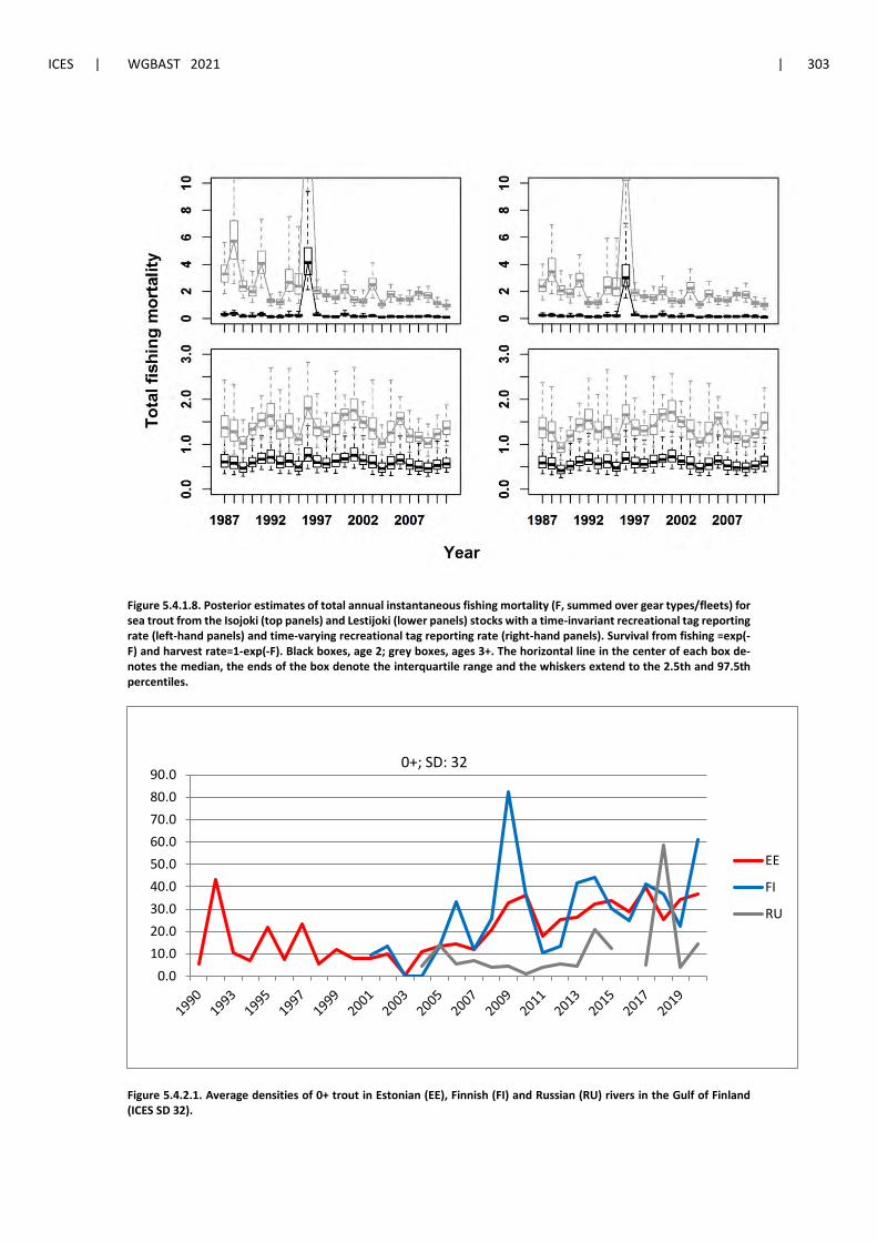
ICES | WGBAST 2021 | 303
Figure 5.4.1.8. Posterior estimates of total annual instantaneous fishing mortality (F, summed over gear types/fleets) for sea trout from the Isojoki (top panels) and Lestijoki (lower panels) stocks with a time-invariant recreational tag reporting rate (left-hand panels) and time-varying recreational tag reporting rate (right-hand panels). Survival from fishing =exp(-F) and harvest rate=1-exp(-F). Black boxes, age 2; grey boxes, ages 3+. The horizontal line in the center of each box de-notes the median, the ends of the box denote the interquartile range and the whiskers extend to the 2.5th and 97.5th percentiles.
Figure 5.4.2.1. Average densities of 0+ trout in Estonian (EE), Finnish (FI) and Russian (RU) rivers in the Gulf of Finland (ICES SD 32).
0.010.020.030.040.050.060.070.080.090.0
EE
FI
RU
0+; SD: 32
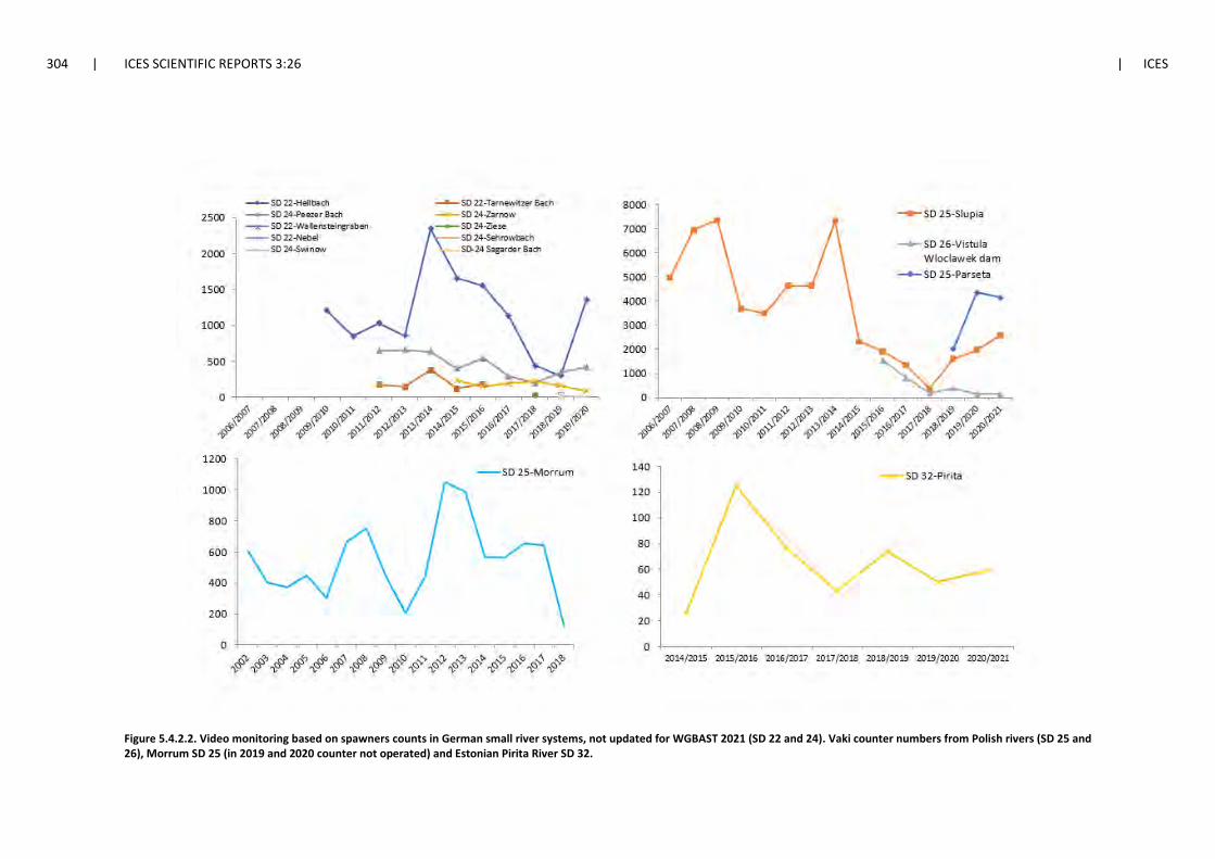
304 | ICES SCIENTIFIC REPORTS 3:26 | ICES
Figure 5.4.2.2. Video monitoring based on spawners counts in German small river systems, not updated for WGBAST 2021 (SD 22 and 24). Vaki counter numbers from Polish rivers (SD 25 and 26), Morrum SD 25 (in 2019 and 2020 counter not operated) and Estonian Pirita River SD 32.
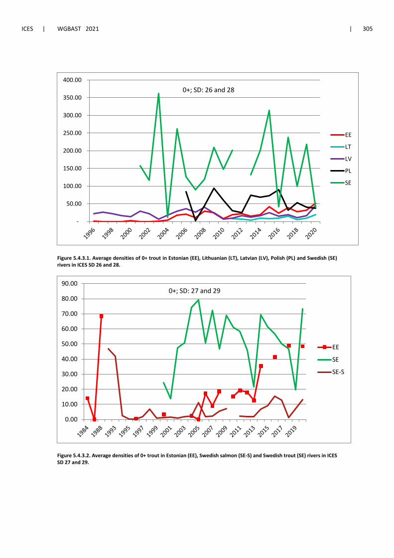
ICES | WGBAST 2021 | 305
Figure 5.4.3.1. Average densities of 0+ trout in Estonian (EE), Lithuanian (LT), Latvian (LV), Polish (PL) and Swedish (SE) rivers in ICES SD 26 and 28.
Figure 5.4.3.2. Average densities of 0+ trout in Estonian (EE), Swedish salmon (SE-S) and Swedish trout (SE) rivers in ICES SD 27 and 29.
-
50.00
100.00
150.00
200.00
250.00
300.00
350.00
400.00
EE
LT
LV
PL
SE
0+; SD: 26 and 28
0.00
10.00
20.00
30.00
40.00
50.00
60.00
70.00
80.00
90.00
EE
SE
SE-S
0+; SD: 27 and 29
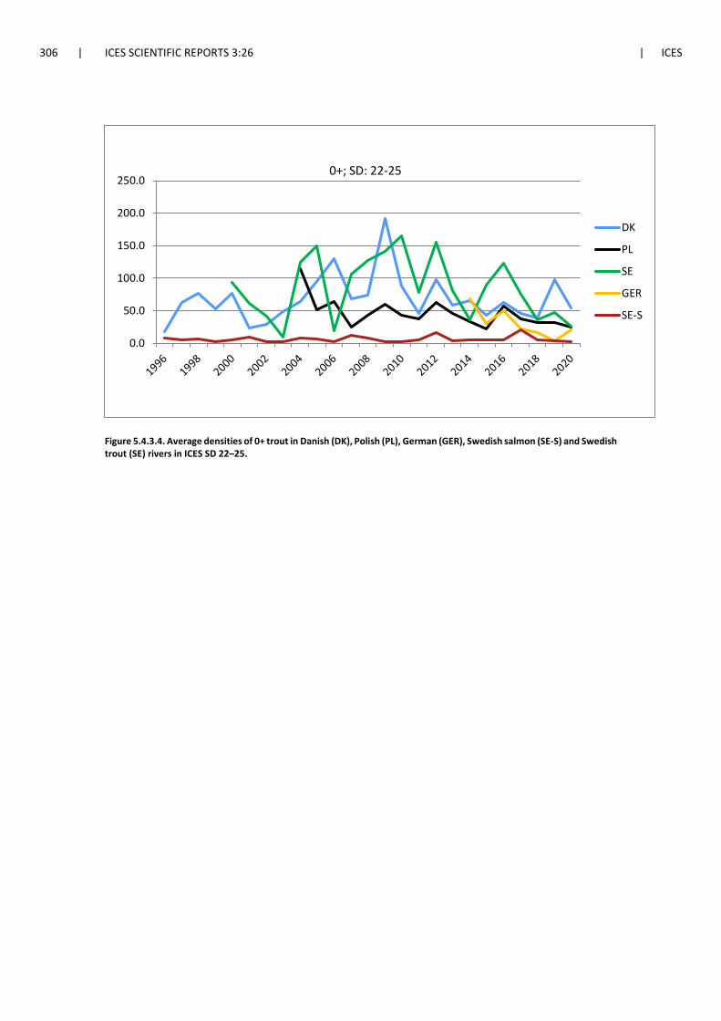
306 | ICES SCIENTIFIC REPORTS 3:26 | ICES
Figure 5.4.3.4. Average densities of 0+ trout in Danish (DK), Polish (PL), German (GER), Swedish salmon (SE-S) and Swedish trout (SE) rivers in ICES SD 22–25.
0.0
50.0
100.0
150.0
200.0
250.0
DK
PL
SE
GER
SE-S
0+; SD: 22-25
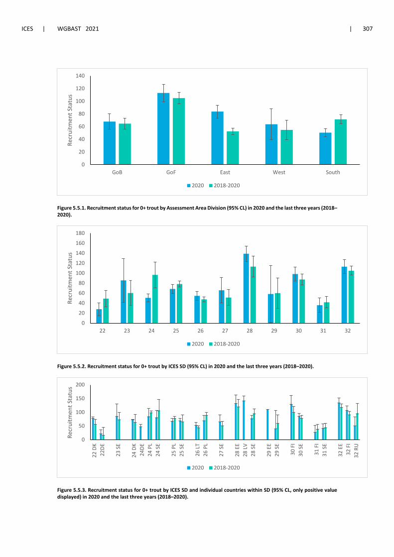
ICES | WGBAST 2021 | 307
Figure 5.5.1. Recruitment status for 0+ trout by Assessment Area Division (95% CL) in 2020 and the last three years (2018–2020).
Figure 5.5.2. Recruitment status for 0+ trout by ICES SD (95% CL) in 2020 and the last three years (2018–2020).
Figure 5.5.3. Recruitment status for 0+ trout by ICES SD and individual countries within SD (95% CL, only positive value displayed) in 2020 and the last three years (2018–2020).
0
20
40
60
80
100
120
140
GoB GoF East West South
Recr
uitm
ent S
tatu
s
2020 2018-2020
0
20
40
60
80
100
120
140
160
180
22 23 24 25 26 27 28 29 30 31 32
Recr
uitm
ent S
tatu
s
2020 2018-2020
0
50
100
150
200
22 D
K22
DE
23 S
E
24 D
K24
DE24
PL
24 S
E
25 P
L25
SE
26 L
T26
PL
27 S
E
28 E
E28
LV
28 S
E
29 E
E29
SE
30 F
I30
SE
31 F
I31
SE
32 E
E32
FI
32 R
U
Recr
uitm
ent S
tatu
s
2020 2018-2020
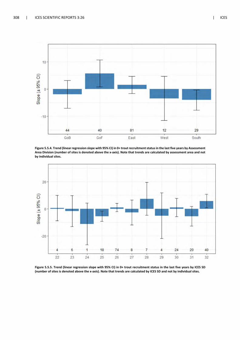
308 | ICES SCIENTIFIC REPORTS 3:26 | ICES
Figure 5.5.4. Trend (linear regression slope with 95% CI) in 0+ trout recruitment status in the last five years by Assessment Area Division (number of sites is denoted above the x-axis). Note that trends are calculated by assessment area and not by individual sites.
Figure 5.5.5. Trend (linear regression slope with 95% CI) in 0+ trout recruitment status in the last five years by ICES SD (number of sites is denoted above the x-axis). Note that trends are calculated by ICES SD and not by individual sites.
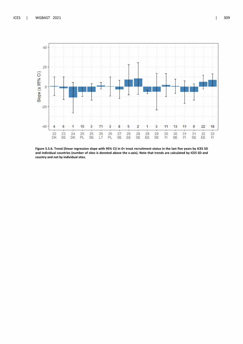
ICES | WGBAST 2021 | 309
Figure 5.5.6. Trend (linear regression slope with 95% CI) in 0+ trout recruitment status in the last five years by ICES SD and individual countries (number of sites is denoted above the x-axis). Note that trends are calculated by ICES SD and country and not by individual sites.
310 | ICES SCIENTIFIC REPORTS 3:26 | ICES
6 References
6.1 Literature
Airaksinen, R., Jestoi, M., Keinänen, M., Kiviranta, H., Koponen, J., Mannio, J., Myllylä, T., Nieminen, J., Raitaniemi, J., Rantakokko, P., Ruokojärvi, P., Venäläinen, E.-R. and Vuorinen, P. J. 2018. Muutokset kotimaisen luonnonkalan ympäristömyrkkypitoisuuksissa (EU-kalat III). Valtioneuvoston selvitys- ja tutkimustoiminnan julkaisusarja 51/2018, 71 pp. (In Finnish with English abstract).
Araki, H. and Schmid, C. 2010. Is hatchery stocking a help or harm? Evidence, limitations and future di-rections in ecological and genetic surveys. Aquaculture, 308: Supplement 1, S2–S11.
Axén, C., Sturve, J., Weichert, F., Leonardsson, K., Hellström, G., Alanärä, A. 2019. Fortsatta undersökningar av laxsjuklighet under 2018. Rapport till Havs- och vattenmyndigheten 2019-03-15. 43 pp. (In Swedish).
Baltic Sea Salmon Foundation (2021). Förvaltningen av svenska Östersjölaxälvar 2020 (In Swedish). 37 pp.
Bartel, R., Bernaś, R., Grudniewska, J., Jesiołowski, M., Kacperska, B., Marczyński, A., Pazda, R., Pender, R., Połomski, S., Skóra, M., Sobocki, M., Terech-Majewska, E. and Wołyński, P. 2009. Wrzodzienica u łososi Salmo salar i troci Salmo trutta trutta w Polsce w latach 2007–2008 (Furunculosis in salmon Salmo salar and sea trout Salmo trutta trutta in Poland in 2008-2008). Komunikaty Rybackie, 3: 7–12 (in Polish with English summary).
Bergkvist, P och Aune, M. 2020. Dioxiner och PCB i lax och öring från Östersjön 2014 till 2019 (In Swedish). PM, Livsmedelsverket. Uppsala. 18 pp.
Börjeson, H. 2013. Redovisning av M74-förekomsten i svenska kompensationsodlade laxstammar från Östersjön för kläckårgång 2011. 4 pp.
Dannewitz J., Palm S., Kagervall A., Whitlock R. and Dahlgren E. 2020a. Svenska laxbestånd i Östersjön – status, exploatering och förvaltning. Biologiskt underlag från Sveriges lantbruksuniversitet (SLU), 54 pp (in Swedish).
Dannewitz J., Palm S., Whitlock R., Larsson S. and Fredriksson R. 2020b. Biologisk rådgivning inför översyn av bestämmelser för fiske med fasta redskap efter lax och andra arter längs norrlandskusten. Biologiskt underlag från Sveriges lantbruksuniversitet (SLU), 56 pp (in Swedish).
Dębowski P. 2018. The largest Baltic population of sea trout (Salmo trutta L.): its decline, restoration at-tempts, and current status. Fisheries & Aquatic Life, 26: 81–100.
EC. 2020. Withdrawal of Commission proposals 2020/CFF 321/03. In: Official Journal of the European Un-ion. Volume 63, 29.09.2020.
Ejsmond, M. J., N. Blackburn, E. Fridolfsson, P. Haecky, A. Andersson, M. Casini, A. Belgrano, and S. Hylander. 2019. Modeling vitamin B1 transfer to consumers in the aquatic food web. Sci Rep 9:10045.
Fiskhälsan. 2007. Produktion av lax och havsöring baserad på vildfisk från Östersjön och Västerhavet: Kontrollprogram för vissa smittsamma sjukdomar samt utfallet av M74, 2007. Fiskhälsan FH AB, 814 70 Älvkarleby. 10 pp. (In Swedish).
Fohgelberg, P. and Wretling, S. 2015. Kontroll av främmande ämnen i livsmedel 2012–2013. National Food Agency’s report 18-2015. 66 pp (in Swedish with English Abstract).
Gustafsson S. 2010. Migration losses of Atlantic salmon (Salmo salar L.) smolts at a hydropower station area in River Åbyälven, Northern Sweden - Passage fates at a reservoir, a power house and a bypass struc-ture. Master thesis. Swedish University of Agricultural Sciences, Dept. of Wildlife, Fish, and Environ-mental Studies, 21 pp.
Hagen, I.J., Jensen, A.J., Bolstad, G.H., Diserud, O.H, Hindar, K., Lo, H. and Karlsson, S. 2019. Supplemen-tary stocking selects for domesticated genotypes. Nature Communications, 10:199.
ICES | WGBAST 2021 | 311
Hansson, S., Karlsson, L., Ikonen, E., Christensen, O., Mitans, A., Uzars, D., Petersson, E. and Ragnarsson, B. 2001. Stomach analyses of Baltic salmon from 1959–1962 and 1994–1997: possible relations between diet and yolk-sac-fry mortality (M74). Journal of Fish Biology, 58: 1730–1745.
Huusko R, Jaukkuri M, Hellström G, Söderberg L, Palm S, Romakkaniemi A. 2020. Spawning migration behavior of salmon and sea trout in the Tornionjoki river system: interim report 2018‒2019. Natural resources and bioeconomy studies 78/2020. 29 pp.
ICES. 2000. Report of the Baltic Salmon and Trout Working Group ICES Doc. CM 2000/ACFM:12.
ICES. 2003. ACFM:12. Report of the Workshop on Catch Control, Gear Description and Tag Reporting in Baltic Salmon (WKCGTS), Svaneke, Denmark 26–28 January 2003.
ICES. 2008a. Report of the Baltic Salmon and Trout Assessment Working Group (WGBAST). ICES CM 2008/ACOM:05.
ICES. 2008b. Report of the Study Group on data requirements and assessment needs for Baltic Sea trout [SGBALANST], by correspondence, December 2007–February 2008. ICES CM 2008/DFC:01. 74 pp.
ICES. 2008c. Report of the Workshop on Baltic Salmon Management Plan Request (WKBALSAL), 13–16 May 2008, ICES, Copenhagen, Denmark. ICES CM 2008/ACOM:55. 61 pp.
ICES. 2009a. Report of the Baltic Salmon and Trout Assessment Working Group (WGBAST), 24–31 March 2009, Oulu, Finland. ICES CM 2009/ACOM:05. 280 pp.
ICES. 2009b. Report of the Study Group on data requirements and assessment needs for Baltic Sea trout [SGBALANST], 3–5 February 2009, Copenhagen, Denmark, ICES 2009/DFC:03. 97 pp.
ICES. 2010. Report of the Working Group on Baltic Salmon and Trout (WGBAST), 24–31 March 2010, St Petersburg, Russia. ICES CM 2010/ACOM:08. 253 pp.
ICES. 2011. Report of the Baltic Salmon and Trout Assessment Working Group (WGBAST), 22–30 March 2011, Riga, Latvia. ICES 2011/ACOM:08. 297 pp.
ICES. 2012. Report of the Baltic Salmon and Trout Assessment Working Group (WGBAST), 15–23 March 2012, Uppsala, Sweden. ICES 2012/ACOM:08. 353 pp.
ICES. 2013. Report of the Baltic Salmon and Trout Assessment Working Group (WGBAST), 3–12 April 2013, Tallinn, Estonia. ICES CM 2013/ACOM:08. 334 pp.
ICES. 2014. Report of the Baltic Salmon and Trout Assessment Working Group (WGBAST), 26 March–2 April 2014, Aarhus, Denmark. ICES CM 2014/ACOM:08. 347 pp.
ICES. 2015. Report of the Baltic Salmon and Trout Assessment Working Group (WGBAST), 23–31 March 2015, Rostock, Germany. ICES CM 2015/ACOM:08. 362 pp.
ICES. 2016a. Report of the Baltic Salmon and Trout Assessment Working Group (WGBAST), 30 March–6 April 2016, Klaipeda, Lithuania. ICES CM 2016/ACOM:09. 257 pp.
ICES. 2016b. ICES Advice on fishing opportunities, catch, and effort, North Atlantic. ICES Advice 2016, Book 10.
ICES. 2017a. Report of the Baltic Salmon and Trout Assessment Working Group (WGBAST), 27 March–4 April 2017, Gdańsk, Poland. ICES CM 2017/ACOM:10. 298 pp.
ICES. 2017b. Report of the Baltic fisheries assessment working group (WGBFAS), 19–26 April 2017, Copen-hagen, Denmark. ICES CM 2017/ACOM:11. 810 pp.
ICES. 2017c. Report of the Benchmark Workshop on Baltic Salmon (WKBALTSalmon), 30 January–3 Febru-ary 2017, Copenhagen, Denmark. ICES CM 2017/ACOM:31. 112 pp.
ICES. 2018a. Report of the Baltic Salmon and Trout Assessment Working Group (WGBAST), 20–28 March 2018, Turku, Finland. ICES CM 2018/ACOM:10. 369 pp.
ICES. 2018b. EU request to review the list of Baltic Sea wild salmon rivers in Annex I of the EC Multiannual plan on Baltic Sea Salmon. In Report of the ICES Advisory Committee, 2018. ICES Advice 2018, sr.2018.09 – https://doi.org/10.17895/ices.pub.4381.
312 | ICES SCIENTIFIC REPORTS 3:26 | ICES
ICES. 2019. Baltic Salmon and Trout Assessment Working Group (WGBAST). ICES Scientific Reports. 1:23. 312 pp. http://doi.org/10.17895/ices.pub.4979.
ICES. 2020a. Baltic Salmon and Trout Assessment Working Group (WGBAST). ICES Scientific Reports. 2:22. 261 pp. http://doi.org/10.17895/ices.pub.5974
ICES. 2020b. Workshop on Baltic Salmon Management Plan (WKBaltSalMP). ICES Scientific Reports. 2:35. 101 pp. http://doi.org/10.17895/ices.pub.5972
ICES. 2020c. ICES Special Request Advice, Baltic Sea ecoregion. ICES Advice 2020–sr.2020.02–https://doi.org/10.17895/ices.advice.6008
Isometsä, K., Orell, P., Romakkaniemi, A., Vähä, V. and Lilja, J. 2021. Tornionjoen nousulohien kai-kuluotausseurannat vuosina 2009–2020. (Hydroacoustic monitoring of the Tornionjoki salmon spawn-ing runs in 2009-2020). Luonnonvara- ja biotalouden tutkimus 9/2021. Luonnonvarakeskus. Helsinki. 32 s. (In Finnish with English abstract).
Jacobson, P., Gårdmark, A., Östergren, J., Casini, M. and Huss, M. 2018. Size-dependent prey availability affects diet and performance of predatory fish at sea: a case study of Atlantic salmon. Ecosphere 9: 1–13.
Jacobson, P., Gårdmark, A., and Huss, M. 2020. Population and size-specific distribution of Atlantic salmon Salmo salar in the Baltic Sea over five decades. Journal of Fish Biology, 96: 408–417.
Jones, S., Kim, E. and Bennett, W. 2008. Early development of resistance to the salmon louse, Lepeophtheirus salmonis (Krøyer), in juvenile pink salmon, Oncorhynchus gorbuscha (Walbaum). Journal of Fish Dis-ease, 31: 591–600.
Kagervall A., Palm S. and Dannewitz J. 2020. Biologisk rådgivning med fokus på ändrade bestämmelser för fiske i älvar i Norrland. Biologiskt underlag från Sveriges lantbruksuniversitet (SLU), 14 pp (in Swedish).
Kallio-Nyberg, I., Romakkaniemi, A., Jokikokko, E., Saloniemi, I., and Jutila, E. 2015. Differences between wild and reared Salmo salar stocks of two northern Baltic Sea rivers. Fisheries Research, 165: 85–95.
Karlsson, L., Ikonen, E., Mitans, A. and Hansson, S. 1999. The diet of salmon (Salmo salar) in the Baltic Sea and connections with the M74 syndrome. Ambio, 28: 37–42.
Keinänen, M., Tolonen, T., Ikonen, E., Parmanne, R., Tigerstedt, C., Rytilahti, J., Soivio, A. and Vuorinen, P. J. 2000. Itämeren lohen lisääntymishäiriö - M74 (English abstract: Reproduction disorder of Baltic salmon (the M74 syndrome): research and monitoring.). In Riista- ja kalatalouden tutkimuslaitos, Kalatutkimuksia - Fiskundersökningar 165, 38 pp.
Keinänen, M., Uddström, A., Mikkonen, J., Rytilahti, J., Juntunen, E.-P., Nikonen, S. and Vuorinen, P. J. 2008. Itämeren lohen M74-oireyhtymä: Suomen jokien seurantatulokset kevääseen 2007 saakka. (Eng-lish abstract: The M74 syndrome of Baltic salmon: the monitoring results from Finnish rivers up until 2007). Riista- ja kalatalous - Selvityksiä 4/2008, 21 pp.
Keinänen, M., Uddström, A., Mikkonen, J., Casini, M., Pönni, J., Myllylä, T., Aro, E. and Vuorinen, P. J. 2012. The thiamine deficiency syndrome M74, a reproductive disorder of Atlantic salmon (Salmo salar) feed-ing in the Baltic Sea, is related to the fat and thiamine content of prey fish. ICES Journal of Marine Science, 69: 516−528.
Keinänen, M., Iivari, J., Juntunen, E.-P., Kannel, R., Heinimaa, P., Nikonen, S., Pakarinen, T., Romakkaniemi, A. and Vuorinen, P. J. 2014. Thiamine deficiency M74 of salmon can be prevented. Riista- ja kalatalous - Tutkimuksia ja selvityksiä 14/2014, 41 pp. (In Finnish with English abstract).
Keinänen, M., Käkelä, R., Ritvanen, T., Pönni, J., Harjunpää, H., Myllylä, T. and Vuorinen, P. J. 2018. Fatty acid signatures connect thiamine deficiency with the diet of the Atlantic salmon (Salmo salar) feeding in the Baltic Sea. Marine Biology, 165: 161.
Koljonen, M.-L., and McKinnell, S. 1996. Assessing seasonal changes in stock composition of Atlantic salmon catches in the Baltic Sea with genetic stock identification. Journal of Fish Biology, 49: 998–1018.

ICES | WGBAST 2021 | 313
Koljonen, M.-L., and Pella, J. J. 1997. The advantage of using smolt age with allozymes for assessing wild stock contributions to Atlantic salmon catches in the Baltic Sea. ICES Journal of Marine Science, 54: 1015–1030.
Koljonen, M.-L., Pella, J. J., and Masuda, M. 2005. Classical individual assignments versus mixture modeling to estimate stock proportions in Atlantic salmon (Salmo salar) catches from DNA microsatellite data. Canadian Journal of Fisheries and Aquatic Sciences, 62: 2143–2158.
Koljonen, M-L. 2006. Annual changes in the proportions of wild and hatchery Atlantic salmon (Salmo salar) caught in the Baltic Sea. ICES Journal of Marine Science, 63: 1274–1285.
Koljonen, M-L., Gross, R. and Koskiniemi, J. 2014. Wild Estonian and Russian sea trout (Salmo trutta) in Finnish coastal sea trout catches: results of genetic mixed-stock analysis. Hereditas, 151: 177–195.
Lilja, J., Romakkaniemi, A., Stridsman, S., and Karlsson, L. 2010. Monitoring of the 2009 salmon spawning run in River Tornionjoki/Torneälven using Dual-frequency IDentification SONar (DIDSON). A Finn-ish-Swedish collaborative research report. 43 pp.
Lindroth, A. 1977. The smolt migration in the river Mörrumsån (Sweden) 1963–1966. Anadromous and Catadromous Fish Committee, CM 1977/M:8. 11 pp.
Magnusson K., Dannewitz J., Kagervall A. and Palm S. 2020. Svenska havsöringsbestånd på västkusten och i Östersjön – status, exploatering och förvaltning. Biologiskt underlag från Sveriges lantbruksuniversitet (SLU), 35 pp (in Swedish).
Majaneva, S., E. Fridolfsson, M. Casini, C. Legrand, E. Lindehoff, P. Margonski, M. Majaneva, J. Nilsson, G. Rubene, N. Wasmund, and S. Hylander. 2020. Deficiency syndromes in top predators associated with large-scale changes in the Baltic Sea ecosystem. PLoS One 15:e0227714.
Mäntyniemi, S., Romakkaniemi, A. 2002. Bayesian mark–recapture estimation with an application to a salmonid smolt population. Can. J. Fish. Aquat. Sci. 59: 1748–1758. doi:10.1139/F02-146.
Miettinen, A., Palm, S., Dannewitz, J., Lind, E., Primmer, C.R., Romakkaniemi, A., Östergren, J. and Pritchard, V.L. 2021. A large wild salmon stock shows genetic and life history differentiation within, but not between, rivers. Conservation Genetics, 22: 35–51.
Palm, S., Dannewitz, J., Järvi, T., Koljonen, M.-L., Prestegaard, T., and Olsén, K. H. 2008. No indications of Atlantic salmon (Salmo salar) shoaling with kin in the Baltic Sea. Canadian Journal of Fisheries and Aquatic Sciences, 65: 1738–1748.
Pella, J., and Masuda, M. 2001. Bayesian method for analysis of stock mixtures from genetic characters. Fishery Bulletin, 99: 151–167.
Pulkkinen H, Mäntyniemi S. 2013. Maximum survival of eggs as the key parameter of stock–recruit meta-analysis: accounting for parameter and structural uncertainty. Can J Fish Aquat Sci. 70: 527–533.
Raitaniemi, J. (Ed.) 2018. Kalakantojen tila vuonna 2017 sekä ennuste vuosille 2018 ja 2019. Luonnonvara- ja biotalouden tutkimus 36/2018, 101 pp. (In Finnish with table and figure texts in English).
Saloniemi, I., Jokikokko, E., Kallio-Nyberg, I., Jutila, E., and Pasanen, P. 2004. Survival of reared and wild Atlantic salmon smolts: size matters more in bad years. ICES Journal of Marine Science, 61: 782–787.
Säisä, M., Koljonen, M.-L. and Tähtinen, J. 2003. Genetic changes in Atlantic salmon stocks since historical times and the effective population size of a long-term captive breeding programme. Conservation Genetics, 4, 613–627.
SLU Aqua. 2018. Redovisning av M74-förekomsten i svenska kompensationsodlade laxstammar från Östersjön 2018. SLU.aqua.2018.5.4-401 8 pp. (In Swedish).
SVA Statens veterinärmedicinska anstalt. 2017. Sjuklighet och dödlighet i svenska laxälvar under 2014–2016: Slutrapport avseende utredning genomförd 2016 Dnr 2017/59. 58 pp. (In Swedish with English abstract).
Vuori, K., Kiljunen, M., Kanerva, M., Koljonen, M.-L., and Nikinmaa, M. 2012. Stock-specific variation of trophic position, diet and environmental stress markers in Atlantic salmon Salmo salar during feeding migrations in the Baltic Sea. Journal of Fish Biology, 81: 1815–1833.
314 | ICES SCIENTIFIC REPORTS 3:26 | ICES
Vuorinen, P.J. and Keinänen, M. 1999. Environmental toxicants and thiamine in connection with the M74 syndrome in Baltic salmon (Salmo salar). In: B.-E. Bengtsson, C. Hill and S. Nellbring (Eds.), Nordic Research Cooperation on Reproductive Disturbances in Fish. Report from the Redfish project. Te-maNord 1999:530, pp. 25–37.
Vuorinen, P.J., Keinänen, M., Heinimaa, P., Iivari, J., Juntunen, E.-P., Kannel, R., Pakarinen, T. and Romak-kaniemi, A. 2014. M74-oireyhtymän seuranta Itämeren lohikannoissa. RKTL:n työraportteja 41/2014, 24 pp. (In Finnish).
Weichert, F., Axén, C., Förlin, L,. Inostroza, P., Kammannm U., Welling, A., Sturve, J., Asker, N. 2020. A multi-biomarker study on Atlantic salmon (Salmo salar L.) affected by the emerging Red Skin Disease in the Baltic Sea. J. Fish Dieases https://doi.org/10.1111/jfd.13288.
Whitlock, R., Mäntyniemi, S., Palm, S., Koljonen, M.-L., Dannewitz, J. and Östergren, J. 2018. Integrating genetic analysis of mixed populations with a spatially-explicit population dynamics model. Methods in Ecology and Evolution. 9:1017–1035.
Östergren, J., Olsson, J., Bergek, S., Palm, S., Tärnlund, S., Dannewitz, J. and Prestegaard, T. 2014. Stamsammansättning av lax i kustfisket 2013 – genetisk provtagning och analys. Report from the Swe-dish University of Agricultural Sciences (SLU). (In Swedish), 28 pp.
Östergren, J., Lind, E., Palm, S., Tärnlund, S., Prestegaard, T. and Dannewitz, J. 2015. Stamsammansättning av lax i det svenska kustfisket 2013 & 2014 – genetisk provtagning och analys. Report from the Swedish University of Agricultural Sciences (SLU). (In Swedish), 30 pp.
Östergren, J., Blomqvist, C., Dannewitz, J, Palm, S. och Fjälling, A. 2020. Discard mortality of salmon caught in different gears. Report from the Swedish University of Agricultural Sciences (SLU). SLU.aqua.2020.5.5-2. 21 pp.
Östergren J, Palm S, Gilbey J, Spong G, Dannewitz J, Königsson H, Persson J, Vasemägi A. 2021 A century of genetic homogenization in Baltic salmon—evidence from archival DNA. Proc. R. Soc. B 20203147. https://doi.org/10.1098/rspb.2020.3147.
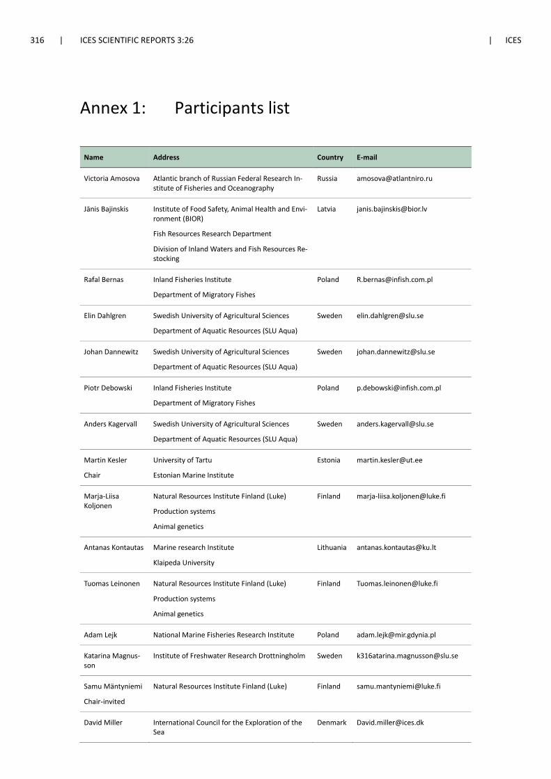
316 | ICES SCIENTIFIC REPORTS 3:26 | ICES
Annex 1: Participants list
Name Address Country E-mail
Victoria Amosova Atlantic branch of Russian Federal Research In-stitute of Fisheries and Oceanography
Russia [email protected]
Jānis Bajinskis Institute of Food Safety, Animal Health and Envi-ronment (BIOR)
Fish Resources Research Department
Division of Inland Waters and Fish Resources Re-stocking
Latvia [email protected]
Rafal Bernas Inland Fisheries Institute
Department of Migratory Fishes
Poland [email protected]
Elin Dahlgren Swedish University of Agricultural Sciences
Department of Aquatic Resources (SLU Aqua)
Sweden [email protected]
Johan Dannewitz Swedish University of Agricultural Sciences
Department of Aquatic Resources (SLU Aqua)
Sweden [email protected]
Piotr Debowski Inland Fisheries Institute
Department of Migratory Fishes
Poland [email protected]
Anders Kagervall Swedish University of Agricultural Sciences
Department of Aquatic Resources (SLU Aqua)
Sweden [email protected]
Martin Kesler
Chair
University of Tartu
Estonian Marine Institute
Estonia [email protected]
Marja-Liisa Koljonen
Natural Resources Institute Finland (Luke)
Production systems
Animal genetics
Finland [email protected]
Antanas Kontautas Marine research Institute
Klaipeda University
Lithuania [email protected]
Tuomas Leinonen Natural Resources Institute Finland (Luke)
Production systems
Animal genetics
Finland [email protected]
Adam Lejk National Marine Fisheries Research Institute Poland [email protected]
Katarina Magnus-son
Institute of Freshwater Research Drottningholm Sweden [email protected]
Samu Mäntyniemi
Chair-invited
Natural Resources Institute Finland (Luke) Finland [email protected]
David Miller International Council for the Exploration of the Sea
Denmark [email protected]
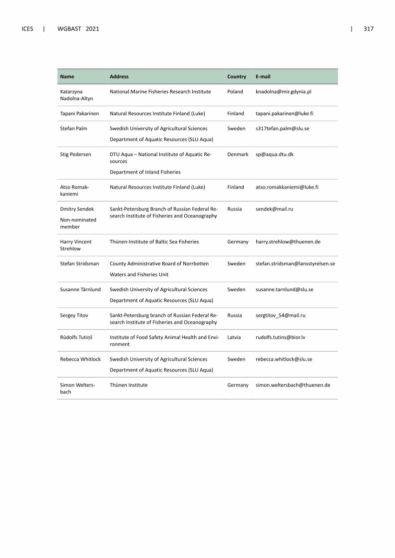
ICES | WGBAST 2021 | 317
Name Address Country E-mail
Katarzyna Nadolna-Altyn
National Marine Fisheries Research Institute Poland [email protected]
Tapani Pakarinen Natural Resources Institute Finland (Luke) Finland [email protected]
Stefan Palm Swedish University of Agricultural Sciences
Department of Aquatic Resources (SLU Aqua)
Sweden [email protected]
Stig Pedersen DTU Aqua – National Institute of Aquatic Re-sources
Department of Inland Fisheries
Denmark [email protected]
Atso Romak-kaniemi
Natural Resources Institute Finland (Luke) Finland [email protected]
Dmitry Sendek
Non-nominated member
Sankt-Petersburg Branch of Russian Federal Re-search Institute of Fisheries and Oceanography
Russia [email protected]
Harry Vincent Strehlow
Thünen-Institute of Baltic Sea Fisheries Germany [email protected]
Stefan Stridsman County Administrative Board of Norrbotten
Waters and Fisheries Unit
Sweden [email protected]
Susanne Tärnlund Swedish University of Agricultural Sciences
Department of Aquatic Resources (SLU Aqua)
Sweden [email protected]
Sergey Titov Sankt-Petersburg branch of Russian Federal Re-search Institute of Fisheries and Oceanography
Russia [email protected]
Rūdolfs Tutiņš Institute of Food Safety Animal Health and Envi-ronment
Latvia [email protected]
Rebecca Whitlock Swedish University of Agricultural Sciences
Department of Aquatic Resources (SLU Aqua)
Sweden [email protected]
Simon Welters-bach
Thünen Institute Germany [email protected]
318 | ICES SCIENTIFIC REPORTS 3:26 | ICES
Annex 2: Stock annex for Salmon (Salmo salar) in subdivisions 22–31 (Main Basin and Gulf of Bothnia) and Subdivision 32 (Gulf of Finland)
The table below provides an overview of the WGBAST Stock Annex. Stock Annexes for other stocks are available on the ICES website Library under the Publication Type “Stock Annexes”. Use the search facility to find a particular Stock Annex, refining your search in the left-hand column to include the year, ecoregion, species, and acronym of the relevant ICES expert group.
Stock ID Stock name Last up-dated
Link
Sal-2431+sal-32
Salmon (Salmo salar) in subdivisions 22–31 (Main Basin and Gulf of Both-nia) and subdivision 32 (Gulf of Finland)
April 2021 Baltic Salmon
ICES | WGBAST 2021 | 319
Annex 3: Recommendations
The Working Group recommends following actions in order to fulfil the shortcomings in the present data and knowledge regarding the Baltic Sea salmon and sea trout to further improve the stock assessment and also, potentially support the management of Baltic salmon and sea trout.
Recommendation Adressed to
1. Catch estimates of recreational salmon and sea trout fisheries are uncertain, incom-plete or totally missing for several countries. Studies and methods to estimate these catches are needed.
ICES Baltic Sea Member States, RCG Baltic Sea (DSG), ICES WGRFS
2. Issues related to salmon sampling:
In Sweden and Finland, in the coastal trapnet fishery, salmon are released back to sea during part of fishing season because of quota fulfillment or fishing regulations. Re-ported and non-reported amounts of these discarded salmon and their survival rate should be evaluated.
Counting of ascending adults should be performed in all salmon index rivers.
Quality of data on amounts and areal distribution of seal damaged salmon and other dead discards by fisheries should be evaluated and improved in countries where these data are found to be defective.
ICES Baltic Sea Member States, RCG Baltic Sea (DSG), ICES PGDATA
3. Issues related to sea trout sampling:
Total population size of 0+ and older parr, as well as estimated total production of smolt should be calculated for rivers where data are available. Especially important are values for index rivers. If possible the areas should be divided into habitat quality clas-ses.
Total production area available for sea trout should be provided for streams where data are available.
Sufficient data coverage of sea trout parr densities from typical trout streams should be collected in all countries. Presently no information was available from Schleswig-Holstein and Kaliningrad region.
Sea trout index rivers should be established to fullfil assessment requirements with re-spect to geographical coverage and data collection needs.
ICES Baltic Sea Member States, RCG Baltic Sea (DSG), ICES PGDATA
4. Data on proportions of sea trout and salmon in catches should be provided to the working group to facilitate estimation of the development of misreporting. ICES Baltic Sea Member States should provide catch composition data from coastal and offshore fisheries (as defined in the EU regulation) covering all main gears.
ICES Baltic Sea Member States
320 | ICES SCIENTIFIC REPORTS 3:26 | ICES
Annex 4: Change in reference points for the sta-tus evaluation of Baltic salmon in as-sessment units 1–4
Background
The European Commission made a request to ICES in 2008 to provide scientific advice on future management of Baltic Sea salmon stocks, in the form of a new management plan to address “all life stages of salmon and all human impacts on salmon”. The request came as the former Salmon Action Plan (SAP) was due to end in 2010. The SAP’s main objective was as follows:
“The production of wild Salmon should gradually increase to attain by 2010 for each Salmon river a nat-ural production of wild Baltic Salmon of at least 50% of the best estimate potential [𝑅𝑅0] and within safe genetic limits, in order to achieve a better balance between wild and reared Salmon.”
Suitable management reference points to replace the 50% 𝑅𝑅0 limit were explored in the Report of the Workshop on Baltic Salmon Management Plan Request (ICES, WKBALSAL 2008). MSY-based ref-erence points were calculated using results from the latest stock assessment (including stock–recruit information). Since many of the rivers assessed by ICES had reached a level of at least 50% of the estimated 𝑅𝑅0 by 2008, it was proposed (ICES, 2008), that the limit of natural smolt production should not be lower than 75% of the estimated 𝑅𝑅0 for each river. Since then, Atlantic salmon stocks in the Baltic Sea have been assessed using 75% of smolt production at the demo-graphic equilibrium with no fishing (𝑅𝑅0 or PSPC) as a proxy for smolt production at maximum sustainable yield (MSY). However, it was already recognized by WKBALSAL that owing to var-iation in river-specific conditions and vital rates, MSY will be achieved at different proportions of 𝑅𝑅0 for different stocks. Hence, using the same proxy for all stocks can be expected to lead to overutilization of some river stocks and underutilization of others. Stock-specific smolt produc-tion at MSY has been calculated earlier using simulation methods (Table 3.4.1.1, ICES, 2008; Table 3.1, ICES, 2017) but was not adopted as a target reference point in assessments.
A few years ago, managers from Baltic Sea countries (BALTFISH) finalized an updated draft of the original EC proposal from 2011. In 2018, ICES received a special request from the EC to eval-uate parts of the plan proposed by BALTFISH. The work to respond to the special request was carried out in an ICES workshop (ICES 2020a, WKBaltSalMP) that included two meetings at-tended by scientific experts, national managers and stakeholder representatives. As requested, existing and alternative reference points for the assessment of stock status and fishing opportu-nities were examined. The existing target formulated in terms of smolt production (75% of 𝑅𝑅0 or PSPC, used as a proxy for MSY), was found to be inconsistent with the overall objective in the draft plan of achieving MSY, since in most cases it does not correspond to the true stock-specific recruitment at MSY (RMSY). A precautionary reference point (Rlim) was further evaluated, defined as the lowest level of smolt production from which a stock is expected to recover to RMSY in one salmon generation, if all fishing was closed (ICES, 2020a). Based on these results, ICES advised use of stock-specific smolt production targets (RMSY and Rlim) as future reference points for Baltic salmon (ICES, 2020b). Reference points for WKBaltSalMP were calculated using the median val-ues of parameters of the Beverton–Holt stock–recruitment function, thus achieving point esti-mates for stock-specific RMSY and Rlim.
ICES | WGBAST 2021 | 321
Reference points in 2021
In 2021, WGBAST evaluated stock status using RMSY and Rlim as reference points. Full distribu-tions for both reference points were derived for each stock in AU 1–4 to be able to evaluate risk (probabilities to reach targets or exceed limits), as has been done with the MSY proxy in earlier years. In deriving full distributions, care was taken to maintain correlations between the refer-ence points and their comparand (in this case smolt abundance).
Methods
Derivations of RMSY and Rlim
Assuming a Beverton–Holt stock–recruitment function, as in the full life-history model for Baltic salmon (FLHM), MSY can be defined as the maximum surplus smolt production, i.e. the maxi-mum difference between the replacement line and stock–recruitment curve. MSY can be found analytically, using the Beverton–Holt function, or using simulations to find the fishing mortality rate that maximizes the average long-term catch. The analytical method was used for derivation of both RMSY and Rlim in the 2021 assessment, although both methods are described below for completeness.
Analytical solution for RMSY
The analytical solution for RMSY makes use of the properties of the Beverton–Holt stock–recruit function. By differentiating the surplus production function (Figure A1b), the egg and smolt production corresponding to MSY can be found at the point where the derivative equals 0 (Fig-ure A1c). This method requires a distribution for 𝑅𝑅0 from simulation, together with posterior distributions for stock-recruit parameters from the FLHM; 𝛼𝛼 (maximum egg survival) and 𝐾𝐾, the maximum recruitment. 𝑅𝑅0 distributions were obtained by running the scenarios code with 0 fishing mortality for 271 years into the future. The average of smolt production over the last 200 years of the simulation was taken as an approximation of 𝑅𝑅0 for each stock. Egg production at the unfished demographic equilibrium 𝐸𝐸0, can then be found as:
𝐸𝐸0 =𝑅𝑅0
�𝛼𝛼 ∗ �1 − 𝑅𝑅0𝐾𝐾 ��
𝐸𝐸𝑀𝑀𝑀𝑀𝑀𝑀 can then be found as:
𝐸𝐸𝑀𝑀𝑀𝑀𝑀𝑀 = −𝛿𝛿 + �(𝛿𝛿2 − 4𝛼𝛼𝛼𝛼)
2𝛼𝛼
where 𝛿𝛿 = 2 𝐾𝐾𝛼𝛼
and 𝛼𝛼 = �𝐾𝐾𝛼𝛼�2− 𝐾𝐾 �𝐾𝐾
𝛼𝛼� �𝐸𝐸0
𝑅𝑅0�. 𝑅𝑅𝑀𝑀𝑀𝑀𝑀𝑀 is then given by:
𝑅𝑅𝑀𝑀𝑀𝑀𝑀𝑀 = 𝐸𝐸𝑀𝑀𝑀𝑀𝑀𝑀𝐾𝐾𝐾𝐾𝛼𝛼 + 𝐸𝐸𝑀𝑀𝑀𝑀𝑀𝑀
In addition to 𝐸𝐸𝑀𝑀𝑀𝑀𝑀𝑀 and 𝑅𝑅𝑀𝑀𝑀𝑀𝑀𝑀, MSY can be found analytically as:
𝑀𝑀𝑀𝑀𝑀𝑀 = 𝑅𝑅𝑀𝑀𝑀𝑀𝑀𝑀 − 𝑅𝑅0𝐸𝐸𝑀𝑀𝑀𝑀𝑀𝑀𝐸𝐸0
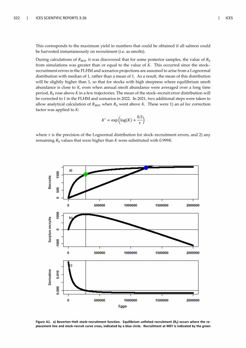
322 | ICES SCIENTIFIC REPORTS 3:26 | ICES
This corresponds to the maximum yield in numbers that could be obtained if all salmon could be harvested instantaneously on recruitment (i.e. as smolts).
During calculations of 𝑅𝑅𝑀𝑀𝑀𝑀𝑀𝑀 it was discovered that for some posterior samples, the value of 𝑅𝑅0 from simulations was greater than or equal to the value of K. This occurred since the stock–recruitment errors in the FLHM and scenarios projections are assumed to arise from a Lognormal distribution with median of 1, rather than a mean of 1. As a result, the mean of this distribution will be slightly higher than 1, so that for stocks with high steepness where equilibrium smolt abundance is close to K, even when annual smolt abundance were averaged over a long time period, 𝑅𝑅0 rose above K in a few trajectories. The mean of the stock–recruit error distribution will be corrected to 1 in the FLHM and scenarios in 2022. In 2021, two additional steps were taken to allow analytical calculation of 𝑅𝑅𝑀𝑀𝑀𝑀𝑀𝑀 when 𝑅𝑅0 went above K. These were 1) an ad hoc correction factor was applied to K:
𝐾𝐾′ = exp �log(𝐾𝐾) +0.5𝜏𝜏�
where 𝜏𝜏 is the precision of the Lognormal distribution for stock–recruitment errors, and 2) any remaining 𝑅𝑅0 values that were higher than K were substituted with 0.999K.
Figure A1. a) Beverton–Holt stock–recruitment function. Equilibrium unfished recruitment (R0) occurs where the re-placement line and stock–recruit curve cross, indicated by a blue circle. Recruitment at MSY is indicated by the green
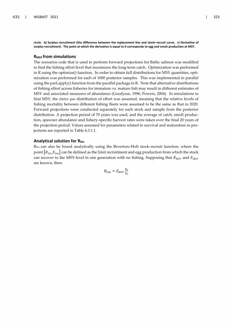
ICES | WGBAST 2021 | 323
circle. b) Surplus recruitment (the difference between the replacement line and stock–recruit curve. c) Derivative of surplus recruitment. The point at which the derivative is equal to 0 corresponds to egg and smolt production at MSY.
RMSY from simulations The scenarios code that is used to perform forward projections for Baltic salmon was modified to find the fishing effort level that maximizes the long-term catch. Optimization was performed in R using the optimize() function. In order to obtain full distributions for MSY quantities, opti-mization was performed for each of 1000 posterior samples. This was implemented in parallel using the parLapply() function from the parallel package in R. Note that alternative distributions of fishing effort across fisheries for immature vs. mature fish may result in different estimates of MSY and associated measures of abundance (Goodyear, 1996; Powers, 2004). In simulations to find MSY, the status quo distribution of effort was assumed, meaning that the relative levels of fishing mortality between different fishing fleets were assumed to be the same as that in 2020. Forward projections were conducted separately for each stock and sample from the posterior distribution. A projection period of 70 years was used, and the average of catch, smolt produc-tion, spawner abundance and fishery-specific harvest rates were taken over the final 20 years of the projection period. Values assumed for parameters related to survival and maturation in pro-jections are reported in Table 4.3.1.1.
Analytical solution for Rlim
Rlim can also be found analytically using the Beverton–Holt stock–recruit function, where the point �𝑅𝑅𝑙𝑙𝑙𝑙𝑙𝑙,𝐸𝐸𝑙𝑙𝑙𝑙𝑙𝑙� can be defined as the limit recruitment and egg production from which the stock can recover to the MSY-level in one generation with no fishing. Supposing that 𝑅𝑅𝑀𝑀𝑀𝑀𝑀𝑀 and 𝐸𝐸𝑀𝑀𝑀𝑀𝑀𝑀 are known, then:
𝑅𝑅𝑙𝑙𝑙𝑙𝑙𝑙 = 𝐸𝐸𝑀𝑀𝑀𝑀𝑀𝑀𝑅𝑅0𝐸𝐸0
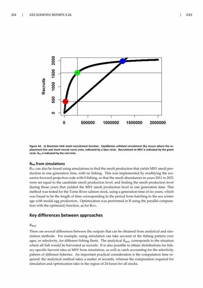
324 | ICES SCIENTIFIC REPORTS 3:26 | ICES
Figure A2. a) Beverton–Holt stock–recruitment function. Equilibrium unfished recruitment (R0) occurs where the re-placement line and stock–recruit curve cross, indicated by a blue circle. Recruitment at MSY is indicated by the green circle. Rlim is indicated by the red circle.
Rlim from simulations Rlim can also be found using simulations to find the smolt production that yields MSY smolt pro-duction in one generation time, with no fishing. This was implemented by modifying the sce-narios forward projection code with 0 fishing, so that the smolt abundances in years 2011 to 2021 were set equal to the candidate smolt production level, and finding the smolt production level during those years that yielded the MSY smolt production level in one generation time. This method was tested for the Torne River salmon stock, using a generation time of six years, which was found to be the length of time corresponding to the period from hatching to the sea winter age with modal egg production. Optimization was performed in R using the parallel computa-tion with the optimize() function, as for RMSY.
Key differences between approaches
𝑅𝑅𝑀𝑀𝑀𝑀𝑀𝑀
There are several differences between the outputs that can be obtained from analytical and sim-ulation methods. For example, using simulation can take account of the fishing pattern over ages, or selectivity, for different fishing fleets. The analytical 𝑅𝑅𝑀𝑀𝑀𝑀𝑀𝑀 corresponds to the situation where all fish would be harvested as recruits. It is also possible to obtain distributions for fish-ery-specific harvest rates at MSY from simulation, as well as catch accounting for the selectivity pattern of different fisheries. An important practical consideration is the computation time re-quired: the analytical method takes a matter of seconds, whereas the computation required for simulation and optimization take in the region of 24 hours for all stocks.
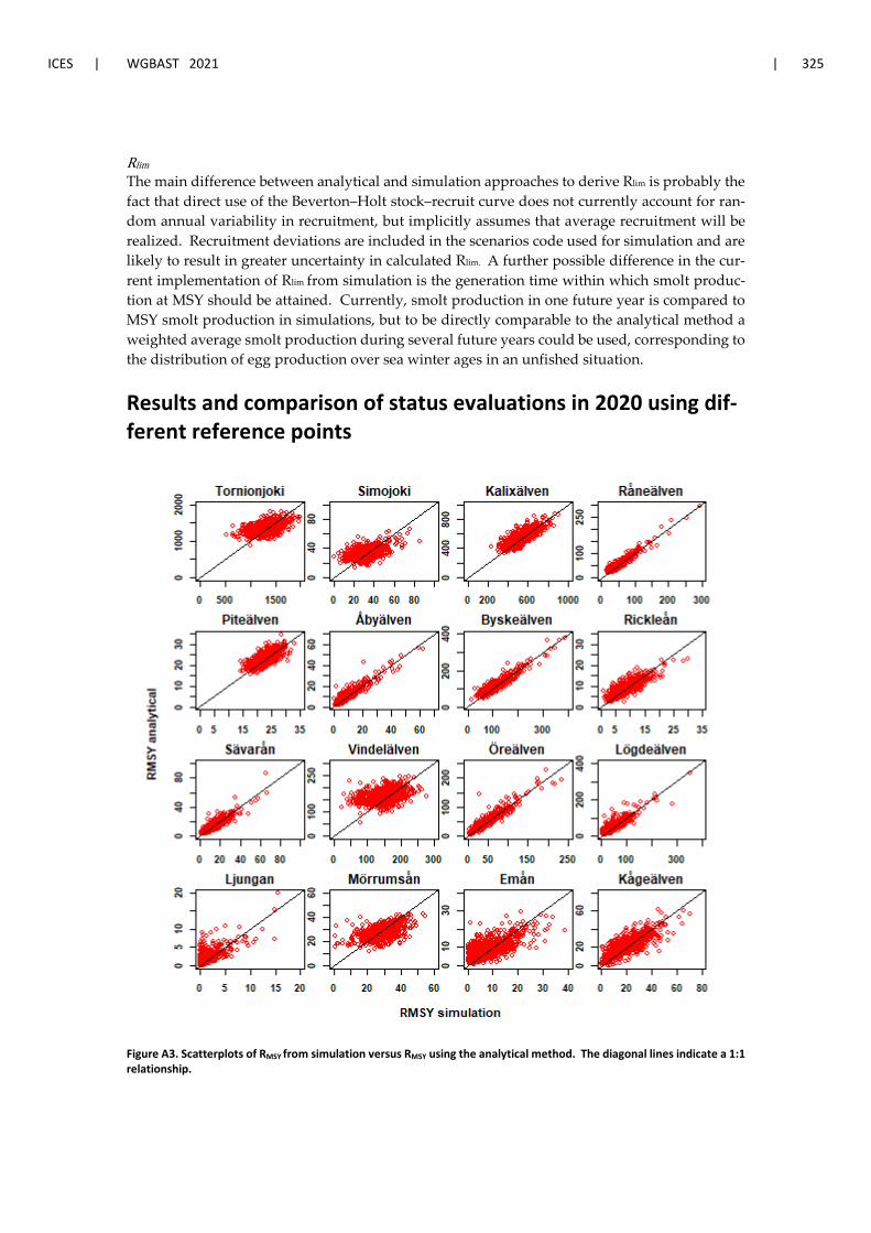
ICES | WGBAST 2021 | 325
Rlim
The main difference between analytical and simulation approaches to derive Rlim is probably the fact that direct use of the Beverton–Holt stock–recruit curve does not currently account for ran-dom annual variability in recruitment, but implicitly assumes that average recruitment will be realized. Recruitment deviations are included in the scenarios code used for simulation and are likely to result in greater uncertainty in calculated Rlim. A further possible difference in the cur-rent implementation of Rlim from simulation is the generation time within which smolt produc-tion at MSY should be attained. Currently, smolt production in one future year is compared to MSY smolt production in simulations, but to be directly comparable to the analytical method a weighted average smolt production during several future years could be used, corresponding to the distribution of egg production over sea winter ages in an unfished situation.
Results and comparison of status evaluations in 2020 using dif-ferent reference points
Figure A3. Scatterplots of RMSY from simulation versus RMSY using the analytical method. The diagonal lines indicate a 1:1 relationship.
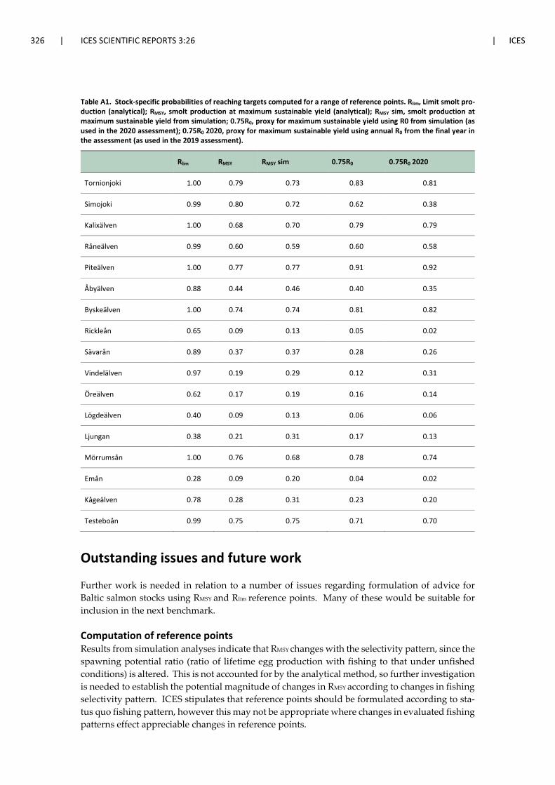
326 | ICES SCIENTIFIC REPORTS 3:26 | ICES
Table A1. Stock-specific probabilities of reaching targets computed for a range of reference points. Rlim, Limit smolt pro-duction (analytical); RMSY, smolt production at maximum sustainable yield (analytical); RMSY sim, smolt production at maximum sustainable yield from simulation; 0.75R0, proxy for maximum sustainable yield using R0 from simulation (as used in the 2020 assessment); 0.75R0 2020, proxy for maximum sustainable yield using annual R0 from the final year in the assessment (as used in the 2019 assessment).
Rlim RMSY RMSY sim 0.75R0 0.75R0 2020
Tornionjoki 1.00 0.79 0.73 0.83 0.81
Simojoki 0.99 0.80 0.72 0.62 0.38
Kalixälven 1.00 0.68 0.70 0.79 0.79
Råneälven 0.99 0.60 0.59 0.60 0.58
Piteälven 1.00 0.77 0.77 0.91 0.92
Åbyälven 0.88 0.44 0.46 0.40 0.35
Byskeälven 1.00 0.74 0.74 0.81 0.82
Rickleån 0.65 0.09 0.13 0.05 0.02
Sävarån 0.89 0.37 0.37 0.28 0.26
Vindelälven 0.97 0.19 0.29 0.12 0.31
Öreälven 0.62 0.17 0.19 0.16 0.14
Lögdeälven 0.40 0.09 0.13 0.06 0.06
Ljungan 0.38 0.21 0.31 0.17 0.13
Mörrumsån 1.00 0.76 0.68 0.78 0.74
Emån 0.28 0.09 0.20 0.04 0.02
Kågeälven 0.78 0.28 0.31 0.23 0.20
Testeboån 0.99 0.75 0.75 0.71 0.70
Outstanding issues and future work
Further work is needed in relation to a number of issues regarding formulation of advice for Baltic salmon stocks using RMSY and Rlim reference points. Many of these would be suitable for inclusion in the next benchmark.
Computation of reference points Results from simulation analyses indicate that RMSY changes with the selectivity pattern, since the spawning potential ratio (ratio of lifetime egg production with fishing to that under unfished conditions) is altered. This is not accounted for by the analytical method, so further investigation is needed to establish the potential magnitude of changes in RMSY according to changes in fishing selectivity pattern. ICES stipulates that reference points should be formulated according to sta-tus quo fishing pattern, however this may not be appropriate where changes in evaluated fishing patterns effect appreciable changes in reference points.
ICES | WGBAST 2021 | 327
Rlim reference points from simulation could also be compared with analytical ones to check the effect of accounting for random variability in recruitment strength and/or a correction could be applied to analytically derived Rlim to account for this.
It was noted in the 2021 assessment that in some simulated future trajectories the stock–recruit steepness dropped below 0.20, meaning that the population could go extinct even in the absence of fishing. Such trajectories accounted for up to ~10% of simulated future trajectories for stocks with low estimated stock–recruit steepness stocks such as Ljungan and Emån. Both the analytical and simulation methods produce an RMSY number for these trajectories. Further investigation is thus needed into evaluated status in such cases, to establish whether these should be excluded from status evaluations, since the concept of MSY is arguably meaningless in such cases. The proportion of simulations where steepness goes below 0.20 could also be reported as an indicator of stock vulnerability to collapse in the absence of fishing, as an additional metric of risk.
Effects of assumed future vital rates on targets Between the 2019 and 2020 assessments, a change was made between using 𝑅𝑅0 from the final year of the assessment, to using 𝑅𝑅0 from long-term simulations in status evaluations. This change was made since by definition, 𝑅𝑅0 is the smolt production at equilibrium which should correspond to a long-term average, rather than reflecting the conditions in any particular year, which would not be realized as the long-term equilibrium value. However, this change has some attendant consequences, namely that the assumed vital rates far ahead in the future used to cal-culate 𝑅𝑅0 do not necessarily reflect current conditions. This can lead to targets that can never be attained with high probability, or conversely, targets that would be met with misleadingly high probability if survival is expected to decline in future. While this is a natural consequence of the assessment framework, review of assumptions about survival rates and other vital rates contrib-uting to lifetime egg production in forward projections, is warranted to ensure that they are based on the best available science and knowledge.
Effects of fishing pattern on generation interval and thereby future projections In 2021, the same generation time within assessment unit groups (seven years for AU 1–3, six years for AU4) was used for different stocks. It is possible that slightly different generation times may be suitable for some stocks where differences in lifetime egg production occur e.g. Ume-Vindelälven. This and possible implications for status evaluations could be checked in a bench-mark.
How many years to use when evaluating current stock status Owing to inherent variation in multiple parameters, estimated smolt production in rivers fluc-tuates from year to year in addition to more long-term trends. So far, WGBAST has focused on smolt production in single years when assessing status. Focusing on average smolt production across several years is expected to result in more stable assessment results, but it remains unclear how many years should be used. As part of a benchmark process, alternative options could be compared and evaluated.
Assessing stock status based on adults rather than smolts In the Baltic Sea region, there is a half-century long tradition of using smolt production as the main metric of abundance, productivity and status of salmon stocks. However, it would be pos-sible to evaluate the MSY and limit reference points for adults instead of smolts (as done for North Atlantic salmon), using either simulation methods, or possibly analytically, given some assumptions to convert egg production to numbers of adult fish. This would mean a move from smolt production targets to spawning stock targets. If this approach would be adopted, then one would expect to see larger interannual variation in the stock status compared to using smolts; spawning stock size is not only influenced by the total abundance of immature fish, but also by
328 | ICES SCIENTIFIC REPORTS 3:26 | ICES
the interannual variation in maturation rates. In order to avoid unnecessary short-term variation in status assessments, using several years’ spawning runs in status assessments would help, as discussed for smolts above.
Assessing status at assessment unit level Probabilities to reach targets at an assessment unit level were computed in the 2021 assessment. The possibility of assessing status at the level of stock complexes (as is done for e.g. North At-lantic salmon stocks) should be given further consideration as an alternative for Baltic salmon stocks, as that would not require every river stock to be above the target with the specified prob-ability. Careful consideration is needed on the details of how this should be implemented, in order that the status assessment and criteria to meet target(s) would be transparent and under-standable.
Effect of level of uncertainty admitted in the assessment The Baltic salmon assessment is comprehensive in the degree of uncertainty admitted. Uncer-tainties are accounted for in nearly all model parameters, as well as in many processes, including post-smolt survival, recruitment, maturation and catchabilities and in observations of data (i.e. sampling error). While Baltic salmon in general is a data-rich system, there are large differences among stocks in the amount of data available. Expert knowledge together with hierarchical structures that allow flow of information between rivers are used to learn about data-poor salmon stocks. There are two important considerations here. Firstly, taking the assessment as a whole, the level of uncertainty admitted is likely exceptional among ICES assessments, which should be taken into account when setting probabilities with which targets should be met. Sec-ondly, there is variation among stocks in the level of uncertainty, such that data-poor stocks can have a lower probability to reach targets regardless of their true status. This could imply that not all stocks should be required to reach the same target within a given time frame.
Formulation of reference points for AU 5–6 stocks Extending the FLHM to include those Baltic salmon stocks (AU 5–6 stocks) which are presently not in FLHM would enable comparable calculations of their stock-specific Rlim and RMSY, and consequent status evaluations. An assessment model for AU 6 has now been developed from most of its parts, but it requires evaluation and checking before it can be used (see details in Appendix 2). The AU 6 model will not be integrated to the AU 1–4 assessment in the first phase, but will be run as a separate unit of stocks. However, the model takes into account migrations of salmon between the assessment units, which will to some extent link the assessments of the AU 1–4 salmon and AU 6 salmon together. For the AU 5 stocks, their inclusion in the same model with the AU 1–4 stocks would be desirable, as AU 5 stocks fulfil their life cycle in the same man-agement area as the AU 1–4 stocks.
References
Goodyear, C. P. 1996. Variability of Fishing Mortality by Age: Consequences for Maximum Sustainable Yield. North America/I Journal of Fisheries Management 16:8–13. 1996.
ICES. 2008. Report of the Workshop on Baltic Salmon Management Plan Request (WKBALSAL), 13–16 May 2008, ICES, Copenhagen, Denmark. ICES CM 2008/ACOM:55. 61 pp.
ICES. 2017. Report of the Benchmark Workshop on Baltic Salmon (WKBALTSalmon), 30 January–3 Febru-ary 2017, Copenhagen, Denmark. ICES CM 2017/ACOM:31. 112 pp.
ICES. 2020a. Workshop on Baltic Salmon Management Plan (WKBaltSalMP). ICES Scientific Reports. 2:35. 101 pp. http://doi.org/10.17895/ices.pub.5972

ICES | WGBAST 2021 | 329
ICES. 2020b. Baltic Salmon and Trout Assessment Working Group (WGBAST). ICES Scientific Reports. 2:22. 261 pp. http://doi.org/10.17895/ices.pub.5974
Powers, J. E. 2004. MSY, Bycatch and Minimization to the “Extent Practicable”. SEDAR7-DW51.
330 | ICES SCIENTIFIC REPORTS 3:26 | ICES
Annex 5: Review of Section 4 “Reference points and assessment of salmon” of the 2021 report of the Baltic Salmon and Trout Assessment Working Group (WGBAST)
The Review Group finds the information in chapter 4 to be clearly presented, scientifically sound and to constitute a good and sufficient basis for ICES to provide advice on fishing opportunities for Baltic salmon stocks.
Review by Eskild Kirkegaard, independent consultant
Overall, I found Section 4 of the WGBAST 2021 report to be well-written, comprehensive and consistent. It contains the information required for ICES to provide advice on the Baltic salmon stocks consistent with ICES framework for advice on fishing opportunities and the reference points recommended by ICES in 2020 in its evaluation of the draft multiannual management plan.
The assessment model used by the Group contains a number of changes compared to the previ-ous one from 2019. The changes seem appropriate and especially the inclusion of the offshore trolling fishery as a separate fishery and the changes allowing the three offshore fisheries (longlining, driftnetting and trolling) to be addressed consistently are valuable, allowing sepa-rate evaluation of the impact of the fisheries on the stocks and catches.
The discussion of the estimation of the smolt production in Section 4.2.2 including the model for estimating M74 mortality is very informative.
In the first paragraph of Section 4.2.3 on the results of the assessment for unit 1–4 stocks, the Group explain how the FHLM was run. I am not able to judge if the approach taken in selecting the most representative chain was appropriate.
The presentation and discussion of the assessment results in Sections 4.2.3, 4.2.4 and 4.2.5 (in-cluding tables and figures) are very comprehensive and informative, and give the reader a good basis for understanding the results and the uncertainties linked to the assessment of the stocks in the different AUs.
The section on projection of AU 1–4 stocks is again comprehensive and informative giving a good description of the assumptions and the results. The ten fishing scenarios presented, seem appropriate.
I am lacking a section addressing the stocks in AU 5 and 6. I recognise that in absence of analytical assessment of the stocks, it may be difficult to comment on future fishing opportunities. How-ever, the Group clearly have good knowledge on the status of the stocks in the two assessment units, and some management considerations for the stocks in AU 5 and 6 are presented in Section 4.5 on future management. It would have been useful with a separate section addressing the future perspectives for these stocks.
Section 4.4 “Additional information affecting perception of stock status” is again very informa-tive and useful in evaluating the quality of the assessments.
I find Section 4.5 on future management of Baltic salmon fisheries very interesting, although not that relevant for the advice on short-term fishing opportunities. The information and the
ICES | WGBAST 2021 | 331
discussions presented in the section would be a good basis for a discussion with ICES clients and stakeholders on future management of Baltic salmon stocks.
Review by Sten Karlsson, independent consultant
I have been asked to review Section 4 as an expert in population genetics of Atlantic salmon, and because of my limited experience and background knowledge of the previous work of ICES on giving fishing advices of Baltic salmon, I regard myself as not qualified for a critical review on many of the issues in the report. Nevertheless, my overall impression is that the Section 4 in the report is well written, and makes use of current knowledge to give the best possible advice for a sustainable fishing of the Baltic salmon.
1. Is the analysis technically correct?
I am not qualified for evaluating all the analyses in the report, but I find the approach of using both genetic assignment and smolt age very solid, and that it makes a crucial contri-bution in approaching stock specific management plans. The inclusion of smolt age data for the genetic assignment increase the power and precision and as pointed out by the authors, it makes it easier to possibly separate between wild and hatchery salmon. The most compre-hensive work on genetic assignment is done for catches in the Gulf of Bothnia, and I expect that there will be more information also from the catches in the rest of the Baltic. So far there are 39 genetic baseline populations used for genetic assignment, and I guess the most im-portant salmon populations are included among these, but it might be a good idea to try to expand this baseline?
2. Is the scope and depth of the science appropriate?
Yes, I find the depth and scope of the science appropriate. It was not clear to me how infor-mation about hatchery or wild origin was included in the advice, and if it is advisable and possible to implement different harvest pressure on these types?
3. Does it contain the knowledge to sufficiently provide the basis for ICES advice?
Yes, the knowledge base is solid and supported by several peer reviewed papers and non-peer reviewed reports.