202

CHAPTER 14 THE LOGISTICS PLANNING PROCESS

3 The MILES module within the LOGWARE software is used to solve this problem. It computes distance based on the great circle distance formula using longitude and latitude. (a) The estimated road distance is 1,380 miles. (b) The estimated road distance is 830 miles. (c) Since both latitudes are in the same hemisphere, no adjustments need to be made.

The estimated distance is 244 miles, or 244×1.61 = 393 km. (d) In this case, one point is east and the other west of the Greenwich line. Therefore, we

need to set a sign convention. Let's set west longitudes as + and east longitudes as −. Thus, 2.20o E longitude is entered into MILES as −2.20 o. The estimated distance is 250 miles, or 250×1.61 = 402.5 km.

4 Suppose that a certain linear grid coordinate system has been overlaid on a map of the United States. The grid numbers are calibrated in miles, and there is a road circuity factor of 1.21. Find the expected road distances between the following pairs of points: Equation 14-1 in the text is used to approximate distances from linear coordinates. The K factor in the equation is set at 1.21. (a) Lansing, MI to Lubbock, TX

D = − + − =121 924 3 1 488 6 1 675 2 2 579 4 1 2902 2. ( . , . ) ( , . , . ) , miles (b) El Paso, TX to Atlanta, GA D = − + − =121 1 696 3 624 9 2 769 3 2 318 7 1 4062 2. ( , . . ) ( , . , . ) , miles (c) Boston, MA to Los Angeles, CA

Location X Coordinate Y Coordinatea. From Lansing, MI 924.3 1675.2

To Lubbock, TX 1488.6 2579.4b. From El Paso, TX 1696.3 2769.3

To Atlanta, GA 624.9 2318.7c. From Boston, MA 374.7 1326.6

To Los Angeles, CA 2365.4 2763.9d. From Seattle, WA 2668.8 1900.8

To Portland, OR 2674.2 2039.7

203

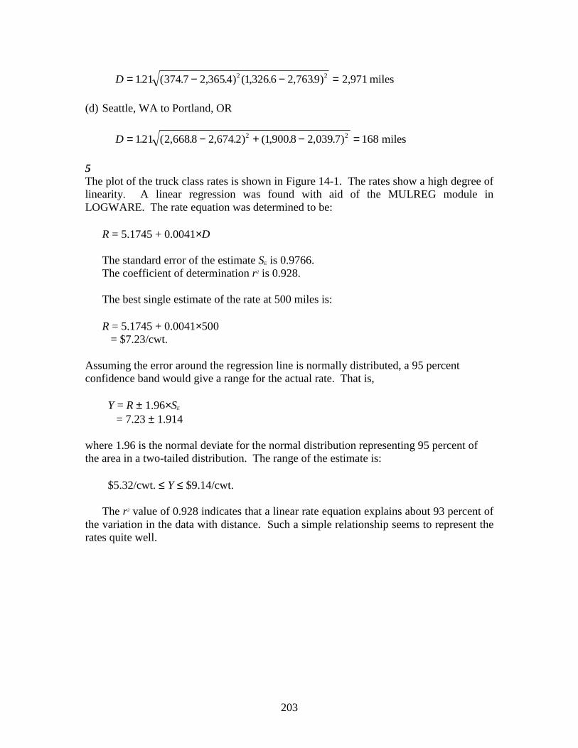
D = − − =121 374 7 2 365 4 1 326 6 2 7639 2 9712 2. ( . , . ) ( , . , . ) , miles (d) Seattle, WA to Portland, OR D = − + − =121 2 668 8 2 674 2 1 900 8 2 039 7 1682 2. ( , . , . ) ( , . , . ) miles 5 The plot of the truck class rates is shown in Figure 14-1. The rates show a high degree of linearity. A linear regression was found with aid of the MULREG module in LOGWARE. The rate equation was determined to be: R = 5.1745 + 0.0041×D The standard error of the estimate SE is 0.9766. The coefficient of determination r2 is 0.928. The best single estimate of the rate at 500 miles is: R = 5.1745 + 0.0041×500 = $7.23/cwt. Assuming the error around the regression line is normally distributed, a 95 percent confidence band would give a range for the actual rate. That is, Y = R ± 1.96×SE = 7.23 ± 1.914 where 1.96 is the normal deviate for the normal distribution representing 95 percent of the area in a two-tailed distribution. The range of the estimate is: $5.32/cwt. ≤ Y ≤ $9.14/cwt. The r2 value of 0.928 indicates that a linear rate equation explains about 93 percent of the variation in the data with distance. Such a simple relationship seems to represent the rates quite well.

204

FIGURE 14-1 Plot of Truck Class Rates

02468

101214161820

0 500 1000 1500 2000 2500 3000 3500

Distance, miles

Cla

ss ra

te, $

/cw

t.

Estimating line

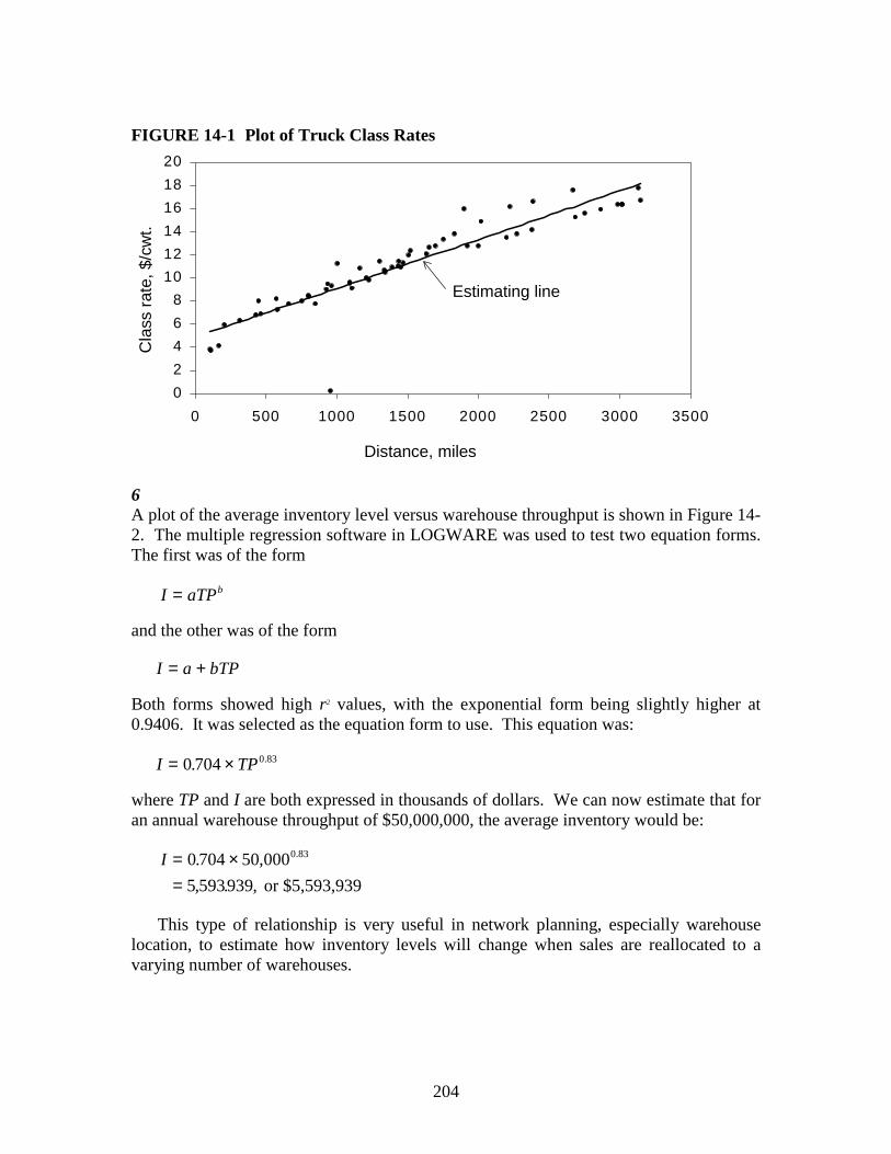
6 A plot of the average inventory level versus warehouse throughput is shown in Figure 14-2. The multiple regression software in LOGWARE was used to test two equation forms. The first was of the form I aTPb= and the other was of the form I a bTP= + Both forms showed high r2 values, with the exponential form being slightly higher at 0.9406. It was selected as the equation form to use. This equation was: I TP= ×0 704 0 83. . where TP and I are both expressed in thousands of dollars. We can now estimate that for an annual warehouse throughput of $50,000,000, the average inventory would be:

I = ×

=0 704 50 0005 593939

0 83. ,, .

.

, or $5,593,939

This type of relationship is very useful in network planning, especially warehouse location, to estimate how inventory levels will change when sales are reallocated to a varying number of warehouses.

205

FIGURE 14-2 Plot of Inventory Levels and Warehouse Throughput for California Fruit Growers’ Association

0

2

4

6

8

10

12

0 20 40 60 80 100

Annual warehouse thruput, $(Millions)

Aver

age

inve

ntor

y le

vel,

$(M

illion

s)

Estimating line

206

USEMORE SOAP COMPANY Teaching Note

The purpose of this case study is to provide students with the opportunity to evaluate and design a large-scale production-distribution network using real data and cost relationships. To assist in the substantial amount of computational effort in this problem, an interactive computer program (WARELOCA) is available in the LOGWARE collection of software modules. Major Issues The text of the case suggests a number of questions that are critical to production-distribution network design. These reduce to three major issues, namely: (1) Should plant capacity be added and, if so, when and where? (2) How many warehouses are optimal and where should they be located? (3) Should the current customer service level be retained? Although no change can be made in the network without potentially affecting other variables, the attempt here will be to treat these questions sequentially to converge on a good network design. Numerous computer runs were made to provide the basic information needed in the analysis. The more meaningful runs are summarized in Appendix A to this note. Tables 1 and 2 compare selected runs for both the current-year and the future-year time periods. This information is used throughout the analysis of the major issues. The Plant Expansion Issue An attempt to meet 5-year growth goals using current plant capacity will cause the system having a total capacity of 1,630,000 cwt. to be out of capacity in 1.7 years. That is,

5th-year demand 1,908,606 cwt. Current demand −1,477,026 Net increase 431,580 cwt.

Therefore, the average annual growth rate is 431,580/5 = 86,316 cwt. So, in (1,630,000 − 1,477,026)/86,316 = 1.7 years all available capacity will be depleted. If no expansion of plant capacity occurs, then 1,908,606 − 1,630,000 = 278,606 cwt. will potentially be lost by the 5th year. Sales are $100 million on 1.477 million cwt. in volume for a product value of $67.7/cwt. With a profit margin of 20 percent, the profit per cwt. would be 20%×$67.7/cwt, or $20/1.477, = $13. Thus, 278,606×13 = $3.16 million are lost in sales. The weighted profit loss over the five-year period would be: 2/5× (0) + ( 3/5)× ((0 + 3.6))/2) = $1.08m/yr.

207

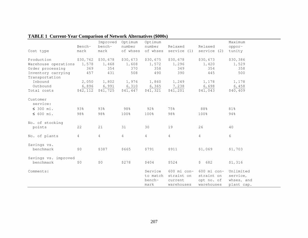
TABLE 1 Current-Year Comparison of Network Alternatives ($000s)

Improved Optimum Optimum MaximumBench- bench- number number Relaxed Relaxed oppor-

Cost type mark mark of whses of whses service (1) service (2) tunity

Production $30,762 $30,678 $30,673 $30,675 $30,678 $30,673 $30,386Warehouse operations 1,578 1,468 1,608 1,572 1,296 1,420 1,529Order processing 369 354 370 358 349 354 358Inventory carrying 457 431 508 490 390 445 500Transportation

Inbound 2,050 1,802 1,976 1,860 1,249 1,178 1,178Outbound 6,896 6,991 6,310 6,365 7,238 6,698 6,458

Total costs $42,112 $41,725 $41,447 $41,321 $41,201 $41,043 $40,409

Customerservice:≤ 300 mi. 93% 93% 98% 92% 75% 88% 81%≤ 600 mi. 98% 98% 100% 100% 98% 100% 94%

No. of stockingpoints 22 21 31 30 19 26 40

No. of plants 4 4 4 4 4 4 6

Savings vs.benchmark $0 $387 $665 $791 $911 $1,069 $1,703

Savings vs. improvedbenchmark $0 $0 $278 $404 $524 $ 682 $1,316

Comments: Service 600 mi con- 600 mi con- Unlimitedto match straint on straint on service,bench- current opt no. of whses, andmark warehouses warehouses plant cap.

208

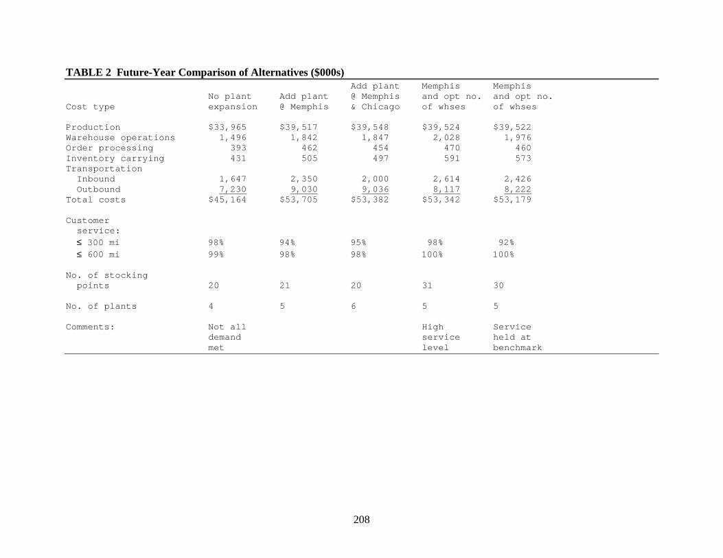
TABLE 2 Future-Year Comparison of Alternatives ($000s) Add plant Memphis Memphis

No plant Add plant @ Memphis and opt no. and opt no.Cost type expansion @ Memphis & Chicago of whses of whses

Production $33,965 $39,517 $39,548 $39,524 $39,522Warehouse operations 1,496 1,842 1,847 2,028 1,976Order processing 393 462 454 470 460Inventory carrying 431 505 497 591 573Transportation

Inbound 1,647 2,350 2,000 2,614 2,426Outbound 7,230 9,030 9,036 8,117 8,222

Total costs $45,164 $53,705 $53,382 $53,342 $53,179

Customerservice:≤ 300 mi 98% 94% 95% 98% 92%≤ 600 mi 99% 98% 98% 100% 100%

No. of stockingpoints 20 21 20 31 30

No. of plants 4 5 6 5 5

Comments: Not all High Servicedemand service held atmet level benchmark

209

Based on a simple rate of return on investment, capturing this profit potential would yield 1.08/4 = 27 percent annually on a $4,000,000 investment for expansion. The return would increase to 90 percent per year with the full loss in the 5th year. The potential seems great enough to justify one unit of expansion (1,000,000 cwt.). Two units of expansion probably cannot be justified, since adequate capacity would be available from the first capacity unit to meet demand requirements. The only benefit would be from the network design improvement. The savings would be about $323,000 per year in the fifth year (see Table 2) comparing one additional plant with two additional plants and keeping the current number of warehouses. The simple return on investment using fifth-year savings would only amount to about 8 percent (323,000×100/4,000,000 = 8.1%). The next question is: Where should the expansion take place at an existing plant or at one of the two proposed locations? From a test of expanding any of the four existing plants or the two proposed plant locations (runs 10 through 16 in Appendix A of this note), it would appear that Memphis would be the lowest cost site in the 5th year with Chicago next at only an additional cost of $76,000 per year (compare runs 14 and 15 in Appendix A). Adding a plant at a new location rather than expanding an existing plant site saves a minimum of $281,000 annually (compare runs 11 and 14 in Appendix A of this note), which results from placing plant capacity closer to warehouses. Selecting Warehouses A simple test on the number of warehouses in the network shows that transportation costs are dropping more rapidly than inventory related costs are increasing (see Figure 1). This means that 40 active warehouses will have the lowest total cost. However, some of these warehouses will have low throughput. In order to maintain a minimum replenishment frequency and shipment size, a minimum throughput needs to be met. Approximately a truckload every two weeks, or 10,400 cwt. of throughput per year, is the minimum activity needed to open a warehouse. Therefore, any warehouse showing less than this throughput will be eliminated from consideration. Under various assumptions about plants and their capacities, demand growth, and service levels, 30 to 31 warehouses seem most economical with no deterioration on service over the benchmark network. The following table shows selected results.

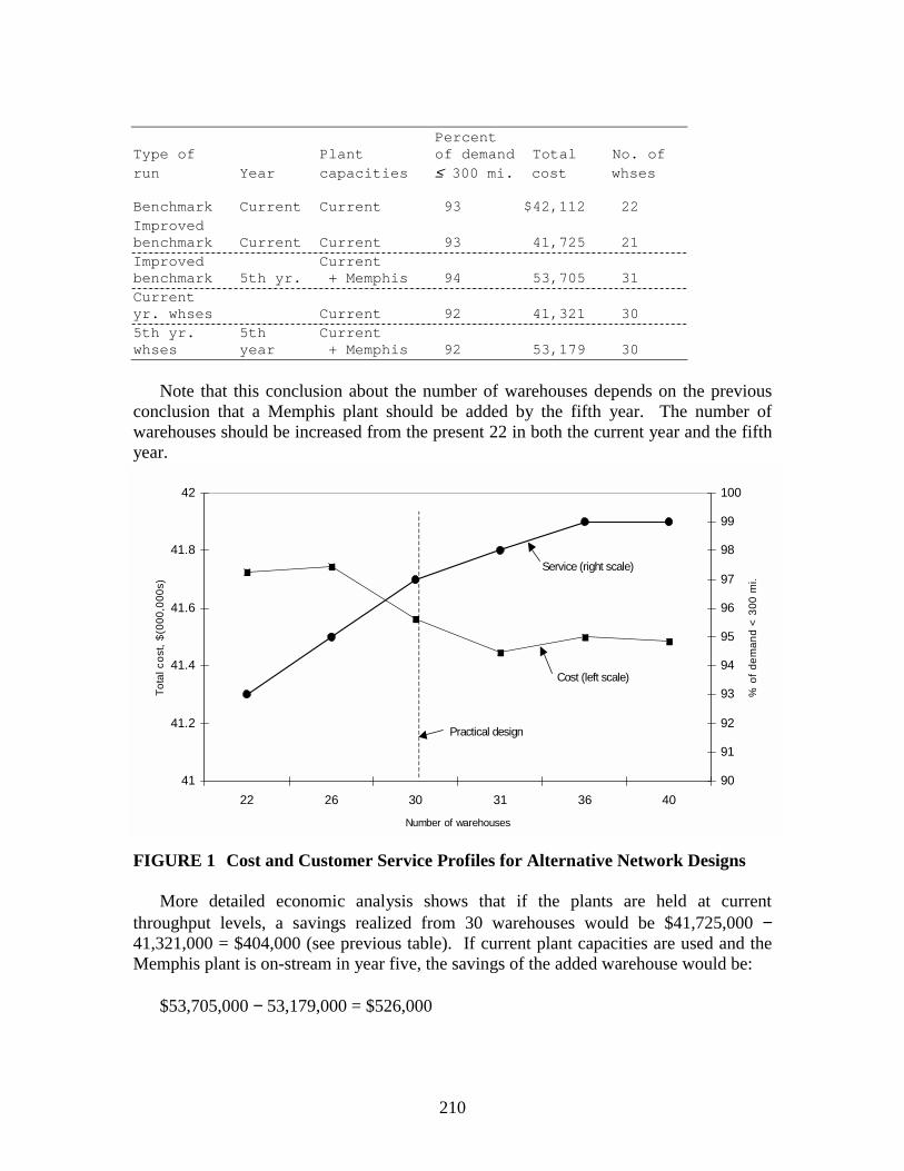
Percent

Type of Plant of demand Total No. ofrun Year capacities ≤ 300 mi. cost whses

Benchmark Current Current 93 $42,112 22Improvedbenchmark Current Current 93 41,725 21Improved Currentbenchmark 5th yr. + Memphis 94 53,705 31Currentyr. whses Current 92 41,321 305th yr. 5th Currentwhses year + Memphis 92 53,179 30

Note that this conclusion about the number of warehouses depends on the previous conclusion that a Memphis plant should be added by the fifth year. The number of warehouses should be increased from the present 22 in both the current year and the fifth year.

42 100

210

FIGURE 1 Cost and Customer Service Profiles for Alternative Network Designs More detailed economic analysis shows that if the plants are held at current throughput levels, a savings realized from 30 warehouses would be $41,725,000 − 41,321,000 = $404,000 (see previous table). If current plant capacities are used and the Memphis plant is on-stream in year five, the savings of the added warehouse would be: $53,705,000 − 53,179,000 = $526,000

41

41.2

41.4

41.6

41.8

22 26 30 31 36 40

Number of warehouses

Tota

l cos

t, $(

000,

000s

)

90

91

92

93

94

95

96

97

98

99

% o

f dem

and

< 30

0 m

i.

Cost (left scale)

Service (right scale)

Practical design

211

On the average, there can be savings of approximately ($404,000 + 526,000)/2 = $465,000 per year by increasing the number of warehouses to 30 from the current 22. Since these are public warehouses, little or no investment would be required to implement the change. Although the number of warehouses remains relatively unchanged from the current year to the 5th year, there is some shifting among the particular warehouses in the mix. The 30 warehouses in the current year should be numbers: 1,2,3,4,5,7,8,11,13,14,15,16,17,18,19,20,21,25,28,31,32,33,34,35,36,37,38,40,44,45 providing that the loading on the current plants is allowed up to the limits of their current capacity. When the Memphis plant is brought on-stream by the end of the second year, the warehouse mix should begin to evolve to numbers: 1,2,3,4,5,7,8,11,13,14,15,17,18,19,20,21,25,28,29,31,32,34,35,36,37,38,40,44,45,47 As the Memphis plant is bought on stream, the Memphis public warehouse is closed and the volume is shifted to the Memphis plant as a warehouse. In addition, the Richmond, VA warehouse is closed and the Las Vegas, NV warehouse is opened. The number of warehouses remains at 30. Both in the base year and in the future year, the throughputs in the plants serving as warehouses are within acceptable limits as the following summary shows. Plant Current- Future-as a Thruput year yearwarehouse limits solution solution

Covington 450,000 cwt. 254,471 cwt. 306,478 cwt.New York 380,000 302,043 380,523Arlington 140,000 66,592 66,161Long Beach 180,000 95,943 117,288

Customer Service Currently, a high proportion of demand (93 percent) is located within 300 miles of a stocking point. Since the service distance may be up to 600 miles and still meet the company's service policy, should the service level be reduced somewhat to effect a cost saving? For example, using the improved benchmark as the base case (run 2), 93 percent of the demand is within 300 miles and 97.5 percent is within 600 miles. If a 600-mile constraint is applied to the current network configuration (run 23), 75 percent of the demand is within 300 miles and 98 percent is still within 600 miles. The total costs are reduced from $41,725,000 to $41,201,000, or a savings of $524,000 per year. In addition, if the number of warehouses in the network is optimized, the costs can be reduced by another $158,000 per year (run 23 vs. run 22). However, $278,000 of the total $524,000 + 158,000 = $628,000 can be realized without a service change. This leaves approximately $404,000 that can be saved by a relaxed service restriction. The question now becomes one of whether the higher costs associated with the more restrictive service level are justified. Since there is no sales-service relationship for this problem, we can only estimate the worth of the service. That is, can enough sales be

212

generated to cover the higher service level? If physical distribution costs for the com-pany are 15 percent of sales, which is probably a conservative estimate, then 1/0.15 = $6.70 in sales must be generated for each dollar that is added to distribution costs. Therefore, to cover $404,000 in cost would require

$404, $6.

$0.,

000 7071 100

38 124×

×=

/ lb. lb./cwt. cwt.

increase in sales. In terms of overall demand, this would be 38,124×100/1,477,026 = 2.5 percent. But not all customers would experience a higher service level. Comparing the demand centers for 299,818 cwt. of demand shows a reduction in warehouse to customer miles. Thus, moving from a minimum cost network to one with a high service level, where the percent of demand less than 300 miles increases from 75 percent to 93 percent, requires that the 38,124 cwt. increase in demand occur in the 299,818 cwt. of demand affected by the change. This would be a 13 percent increase. The products are not highly differentiated from others in the marketplace so that service plays an important role in selling these products. Whether a 93 − 75 = 18 percentage points increase in service can result in a 2.5 percent increase in overall sales cannot be judged by the distribution department alone. The sales department must play an important part in indicating whether the additional sales are possible. If they are not likely to be realized, there is no incentive for a network other than the minimum cost one. If this information is not available from sales, the conclusion is likely to be to maintain the status quo as represented by the benchmark. That is, one-day service is most likely to guide the design. Overall Analysis and Summary The recommended design would involve an immediate increase in the number of warehouses from 22 to 30. In addition, there should be an immediate reallocation of demand among the existing plants. No reduction in the customer service level seems justified at this time. Therefore, a total cost reduction of $42,112,000 − 41,321,000 = $791,000 per year seems immediately achievable (run 1 vs. run 18). By the end of the 2nd year, the Memphis plant should be brought on stream and the network should begin to evolve from the current design (run 24) to that for the fifth year (run 25). The addition of a plant is justified from the high rate of return realized from the profit potential of being able to continue meeting the growth in demand. For the current year, a breakdown of the service and the cost changes show the following:

213

Current-Bench- year Change from

Cost type mark design benchmark

Production $30,762 $30,675 $ -87 -0.3%Whse operations 1,578 1,572 - 6 -0.4Order processing 369 358 -11 -3.0Inventory carrying 457 490 +33 +7.2Transportation

Inbound 2,050 1,860 -190 -9.3Outbound 6,896 6,365 -531 -7.7

Total costs ($000s) $42,112 $41,320 $-792 -1.9%

By the fifth year, total distribution costs should be $53,179,000, or $53,179,000/1,908,606 = $27.86, compared with the current-year cost of 42,112,463/1,477,026 = $28.51 per cwt. If current year costs are projected to the fifth year demand level, the 5th-year production/distribution costs might be 28.51×1,908,606 = $54,414,357, or a savings of $54,414,357 − 53,179,000 = $1,235,357 per year. Of course, these savings can only be realized through the addition of capacity at Memphis for $4,000,000. If this capacity is useful for at least 15 years, the amortization of $4,000,000/15 = $267,000 per year would yield a net savings of $532,000 per year. Overall, the design change appears to be justified.

214

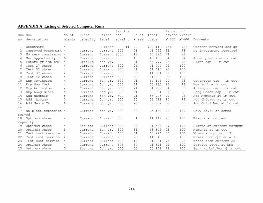
APPENDIX A Listing of Selected Computer Runs Service Percent of

Run.Run No of Plant Demand con- No of Total demand withinno. description plants capacity level straint whses costs ≤ 300 ≤ 600 Comments

1 Benchmark 4 - Current - mi 22 $42,112 93% 98% Current network design2 Improved benchmark 4 Current Current 300 21 41,725 93 98 No investment required3 No serv constraint 4 Current Current 9000 18 40,896 71 894 Max opportunity 6 Current Current 9000 40 40,409 81 94 Added plants at 1m cwt5 Future yr-imp bmk 4 Crnt+1m 5th yr. 300 21 53,777 93 98 Plant cap + 1m cwt6 Test 27 whses 4 Current Current 300 26 41,744 95 1007 Test 32 whses 4 Current Current 300 31 41,615 98 1008 Test 37 whses 4 Current Current 300 36 41,501 99 1009 Test 42 whses 4 Current Current 300 40 41,486 99 100

10 Exp Covington 4 Current 5th yr. 300 21 54,145 94 98 Covington cap + 1m cwt11 Exp New York 4 Current 5th yr. 300 21 53,986 93 98 New York + 1m cwt12 Exp Arlington 4 Current 5th yr. 300 21 54,709 94 98 Arlington cap + 1m cwt13 Exp Long Beach 4 Current 5th yr. 300 21 55,251 94 98 Long Beach cap + 1m cwt14 Add Memphis 5 Current 5th yr. 300 21 53,705 94 98 Add Memphis at 1m cwt15 Add Chicago 5 Current 5th yr. 300 20 53,781 94 98 Add Chicago at 1m cwt16 Add Mem & Chi 6 Current 5th yr. 300 20 53,382 95 98 Add Chi & Mem at 1m cwtea17 No plant expansion 4 Current 5th yr. 300 20 45,164 98 100 Only 85.4% of demndserved18 Optimum whses 4 Current Current 300 31 41,447 98 100 Plants at currentcapacity19 Optimum whses 4 See cmt Current 300 30 41,563 97 100 Plants at current thruput20 Optimum whses 5 Current 5th yr. 300 31 53,342 98 100 Memphis at 1m cwt21 Test cust service 4 Current Current 600 31 40,996 80 100 Whses at opt no = 3122 Test cust service 4 Current Current 600 26 41,043 88 100 Whses from opt no = 3123 Test cust service 4 Current Current 600 19 41,201 75 98 Whses from current 2224 Optimum whses 4 Current Current 375 30 41,321 92 100 Service level at bmk25 Optimum whses 5 See cmt 5th yr. 375 30 53,179 92 100 Serv at bmk/Mem @ 1m cwt

215

ESSEN USA Teaching Note

Strategy Essen USA is concerned with entire supply channel performance. The supply channel consists of four echelons ranging from factory to customers. The purpose of this case study is for the student to manipulate the supply channel variables using a channel simulator in order to improve individual member and system-wide performance. The channel variables include forecasting methods, inventory policies, transportation services, production lot sizes, order processing costs, and stock availability levels. Students should seek to optimize channel performance, although it is not expected that the optimum actually can be found or verified. However, improving performance over existing levels is achievable. The SCSIM module of LOGWARE is used to simulate the demand and product flows throughout the multi-echelon supply chain. SCSIM is an ordinary Monte Carlo day-to-day type of simulator. Using a simulator for performance improvement requires thinking of it in terms of as an experimental methodology. That is, a single run of the simulator is a particular event sequence generated from random numbers. Changing the seed number in the simulator causes a different set of random numbers to be generated and possibly another outcome from the same input data. A simulation run with a specified seed number should be viewed as a single statistical observation and multiple outcomes from various seed numbers should be treated as a statistical sample and analyzed accordingly, i.e., comparing means and standard deviations. Each simulation is run for a period of 11 years with results taken from years 2 through 11. The first year is not used since it can show unstable results due to startup conditions. The results appear to reach steady state by the second year, and the results for the 10 years thereafter are averaged to give a reasonable representation of channel performance for a given run. The database used to represent the current performance of the channel, as derived from the case study, is summarized in the Appendix A of this note and a typical run report is shown in Appendix B. This case provides students with the opportunity to observe the operation of a multi-echelon supply channel and to assess the impact of changing key operating variables on individual members as well as on channel-wide performance. The effect on cost and customer service as well as sales, inventory, and back order levels of demand patterns, demand forecasting methods, inventory control methods, transportation performance, production lot sizing, order processing procedures, and item fill rates can be observed in both graphical and report forms. Most importantly, students can see the effects of supply chain decisions rather than project the results statistically. Questions 1. What can you say about the logistics performance throughout the supply channel for

Essen and its customers?

General observations It is recognized that Essen must deal with demand that has significant seasonal peaks at gift-giving times of the year as shown in Figure 1. Compared with a smooth demand pattern, this can cause increasing demand variability upstream from the customers, as illustrated in Figure 2. This “bull whip” effect is partly a result of the demand for an upstream member being derived from the order size and pattern of its immediate downstream channel member. Forecast accuracy, lead-time uncertainty, and inventory control method also affect demand variability and the resulting cost of that variability.

Figure 1 Typical Demand Pattern for Essen Over the Period of One Year

216

Retailer

Distri-butor

Ware-house Factory

Retailer

FactoryRetailerwarehouse

Essenwarehouse

Retailer

Distri-butor

Ware-house Factory

Retailer

FactoryRetailerwarehouse

Essenwarehouse

Figure 2 Increasing Demand Variability of Upstream Channel Members for a

Four-Year Period

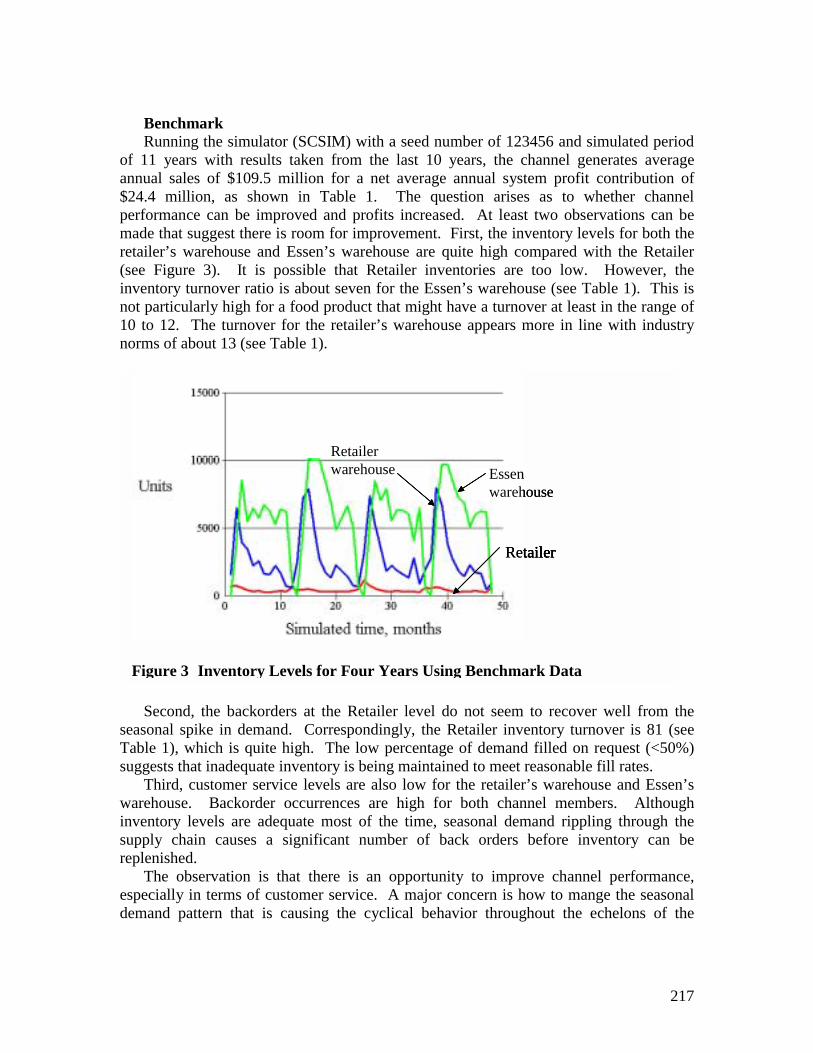
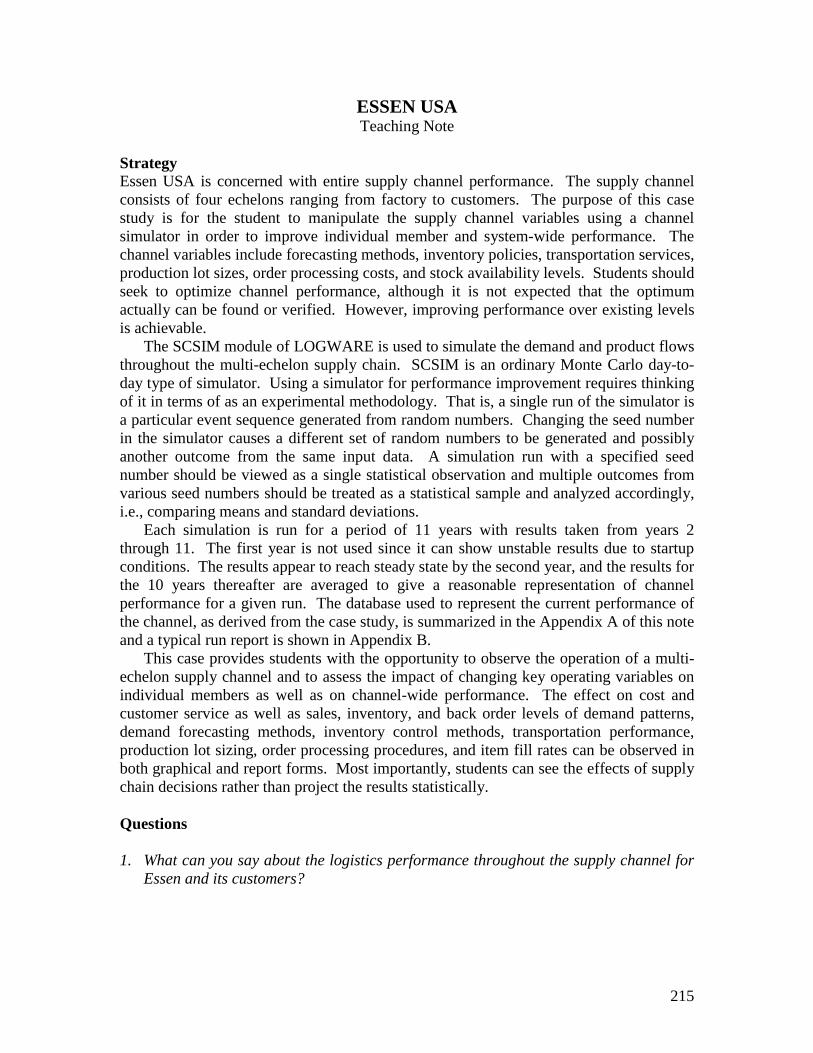
Benchmark Running the simulator (SCSIM) with a seed number of 123456 and simulated period of 11 years with results taken from the last 10 years, the channel generates average annual sales of $109.5 million for a net average annual system profit contribution of $24.4 million, as shown in Table 1. The question arises as to whether channel performance can be improved and profits increased. At least two observations can be made that suggest there is room for improvement. First, the inventory levels for both the retailer’s warehouse and Essen’s warehouse are quite high compared with the Retailer (see Figure 3). It is possible that Retailer inventories are too low. However, the inventory turnover ratio is about seven for the Essen’s warehouse (see Table 1). This is not particularly high for a food product that might have a turnover at least in the range of 10 to 12. The turnover for the retailer’s warehouse appears more in line with industry norms of about 13 (see Table 1).

sTs winsr ed

RetailerRetailer

Retailerwarehouse Essen

warehouse

RetailerRetailer

Retailerwarehouse Essen

warehouse

Figure 3 Inventory Levels for Four Years Using Benchmark Data

217

Second, the backorders at the Retailer level do not seem to recover well from the easonal spike in demand. Correspondingly, the Retailer inventory turnover is 81 (see able 1), which is quite high. The low percentage of demand filled on request (<50%) uggests that inadequate inventory is being maintained to meet reasonable fill rates.

Third, customer service levels are also low for the retailer’s warehouse and Essen’s arehouse. Backorder occurrences are high for both channel members. Although ventory levels are adequate most of the time, seasonal demand rippling through the

upply chain causes a significant number of back orders before inventory can be eplenished.

The observation is that there is an opportunity to improve channel performance, specially in terms of customer service. A major concern is how to mange the seasonal emand pattern that is causing the cyclical behavior throughout the echelons of the

218

channel. Current performance of the channel members is summarized in Table 1 for four simulation runs using different seed numbers.

Channel member Run 1 Run 2 Run 3 Run 4 Average Essen’s factory Total cost $73,105,904 $72,967,088 $72,616,192 $72,477,376 $72,791,640 Units produced 37,918 37,846 37,664 37,592 37,755 Cost per unit $1,928 $1,928 $1,928 $1,928 $1,928 Essen’s warehouse

TO ratio 6.52 6.59 6.61 6.58 6.58 Fill rate <50% <50% <50% <50% <50% Cost $5,578,291 $5,549,202 $5,521,236 $5,540,447 $5,547,294 Cost per unit $147.02 $146.50 $146.32 $146.65 $146.62 Retailer’s warehouse

TO ratio 12.95 13.01 12.96 12.89 12.95 Fill rate <50% <50% <50% <50% <50% Cost $3,873,236 $3,895,406 $3,853,890 $3,912,699 $3,883,808 Cost per unit $101.94 $102.15 $102.14 $103.07 $102.33 Retailer TO ratio 81.02 80.38 80.45 80.60 80.61 Fill rate <50% 53.02% 54.09% <50% <50% Units sold 38,017 37,983 37,774 37,804 37,895 Cost $2,884,527 $2,768,697 $2,939,464 $2,981,607 $2,893,574 Cost per unit $76.19 $72.89 $77.82 $78.87 $76.44 System Profit $24,426,593 $24,591,053 $24,235,498 $24,340,563 $24,398,426 Profit as % of sales 22.23% 22.40% 22.20% 22.28% 22.28% Seed Number 123456 444444 555555 666666 2. What steps would you suggest taking to improve logistics performance throughout the

channel? Do any of the changes involve Essen? If so, does the company directly realize any cost and/or operating performance improvements?

A number of actions can be taken to lower costs and improve customer service. Improving the forecast, shortening the lead times, changing the inventory control policy, and changing production lot sizes are all variables that can be altered for possible performance improvement. The interactions among these variables and the large number of variable combinations preclude finding the optimal set. However, they can be explored in a systematic way to find improvement. The primary focus of this analysis will be to increase the fill rates at the risk of increasing costs. Ultimately, revenues, through improved customer service, may be preserved or increased to more than compensate for reduced profits.

Table 1 Average Annual Performance of Channel Members and the System at Benchmark

219

Retailer Level Start with the retailer because of the proximity to the customer. Fill rates need to be improved, probably in the 95-99% range as specified in the database. Inventory turns can be guided by the industry average of 12 turns per year. Where the two cannot be jointly met, service will prevail. Clearly, putting additional inventory at the retail point will improve customer service. Using the company’s current inventory policy of stocking to demand, the target level can be raised without changing the review time. Exploring different target levels shows 14 days to offer about 35 turns and a 99+% fill rate. Because of the high cost of a back order, total costs at the retail level drop significantly. Altering the forecasting method and the settings associated with the method yield little opportunity for improvement. Using an exponential smoothing model with a high smoothing constant to better follow the seasonal changes in demand results in increased costs. Lowering the smoothing constant to 0.1 did not offer improvement either. Altering the number of periods in the moving average model did not improve costs and only degraded performance. Shortening the review time in the stock-to-demand reorder policy did have a positive effect on fill rate, but resulted in high costs and lower inventory turns. The tradeoff did not seem beneficial, given the fill rate and turnover targets. Retail Warehouse Level Determining an improved policy at this level is difficult because a 95% fill rate and 10 to 12 inventory turns is an illusive goal. Using service as the primary target, a stock-to-demand control policy is used with a review period of 7 days and a target of 25 days of inventory. The forecasting method is moving average with a period of 7 days. The performance achieved at this channel level is about nine inventory turns per year and a 97% fill rate. Essen’s Warehouse Level The performance at Essen’s warehouse level seems to mimic that at the retail warehouse level except that there is more demand variability. Again, an inventory turnover ratio in the target range cannot be achieved while maintaining a high fill rate level. Trying to achieve high service levels with high levels of inventory is difficult, probably due to the extensive demand variability that filters back to this member of the channel. Multiple simulation runs show that a high fill rate cannot consistently be achieved even when on the average inventory levels are high. However, average performance shows an 82% fill rate and 1.5 inventory turns per year based on a 7-day moving average forecasting model and a stock-to-demand inventory control policy with a review time of 7 days and an inventory target of 25 days. Essen’s Factory The concern with the factory level in the channel is whether product should be manufactured in a larger lot size, but with slightly higher production time variability. The reduced costs seem to out weigh the negative effects of increased variability. Producing in the larger lot size is favored.

220

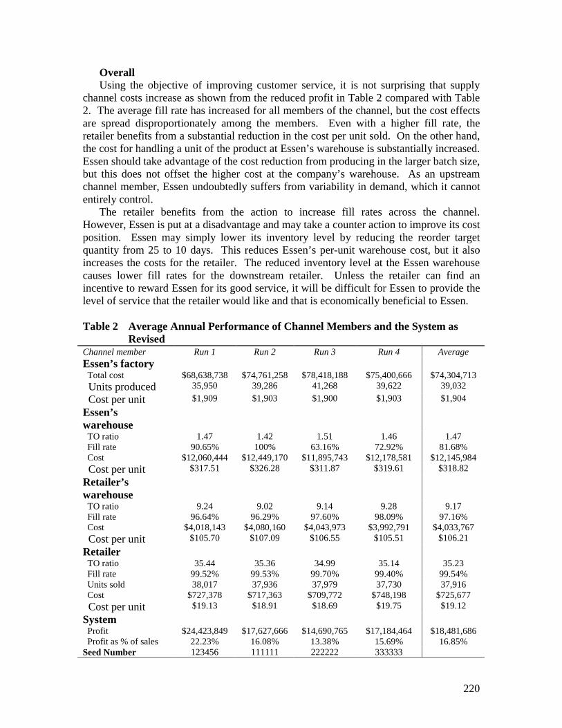
Overall Using the objective of improving customer service, it is not surprising that supply channel costs increase as shown from the reduced profit in Table 2 compared with Table 2. The average fill rate has increased for all members of the channel, but the cost effects are spread disproportionately among the members. Even with a higher fill rate, the retailer benefits from a substantial reduction in the cost per unit sold. On the other hand, the cost for handling a unit of the product at Essen’s warehouse is substantially increased. Essen should take advantage of the cost reduction from producing in the larger batch size, but this does not offset the higher cost at the company’s warehouse. As an upstream channel member, Essen undoubtedly suffers from variability in demand, which it cannot entirely control. The retailer benefits from the action to increase fill rates across the channel. However, Essen is put at a disadvantage and may take a counter action to improve its cost position. Essen may simply lower its inventory level by reducing the reorder target quantity from 25 to 10 days. This reduces Essen’s per-unit warehouse cost, but it also increases the costs for the retailer. The reduced inventory level at the Essen warehouse causes lower fill rates for the downstream retailer. Unless the retailer can find an incentive to reward Essen for its good service, it will be difficult for Essen to provide the level of service that the retailer would like and that is economically beneficial to Essen.

Channel member Run 1 Run 2 Run 3 Run 4 Average Essen’s factory Total cost $68,638,738 $74,761,258 $78,418,188 $75,400,666 $74,304,713 Units produced 35,950 39,286 41,268 39,622 39,032 Cost per unit $1,909 $1,903 $1,900 $1,903 $1,904 Essen’s warehouse

TO ratio 1.47 1.42 1.51 1.46 1.47 Fill rate 90.65% 100% 63.16% 72.92% 81.68% Cost $12,060,444 $12,449,170 $11,895,743 $12,178,581 $12,145,984 Cost per unit $317.51 $326.28 $311.87 $319.61 $318.82 Retailer’s warehouse

TO ratio 9.24 9.02 9.14 9.28 9.17 Fill rate 96.64% 96.29% 97.60% 98.09% 97.16% Cost $4,018,143 $4,080,160 $4,043,973 $3,992,791 $4,033,767 Cost per unit $105.70 $107.09 $106.55 $105.51 $106.21 Retailer TO ratio 35.44 35.36 34.99 35.14 35.23 Fill rate 99.52% 99.53% 99.70% 99.40% 99.54% Units sold 38,017 37,936 37,979 37,730 37,916 Cost $727,378 $717,363 $709,772 $748,198 $725,677 Cost per unit $19.13 $18.91 $18.69 $19.75 $19.12 System Profit $24,423,849 $17,627,666 $14,690,765 $17,184,464 $18,481,686 Profit as % of sales 22.23% 16.08% 13.38% 15.69% 16.85% Seed Number 123456 111111 222222 333333

Table 2 Average Annual Performance of Channel Members and the System as Revised

221

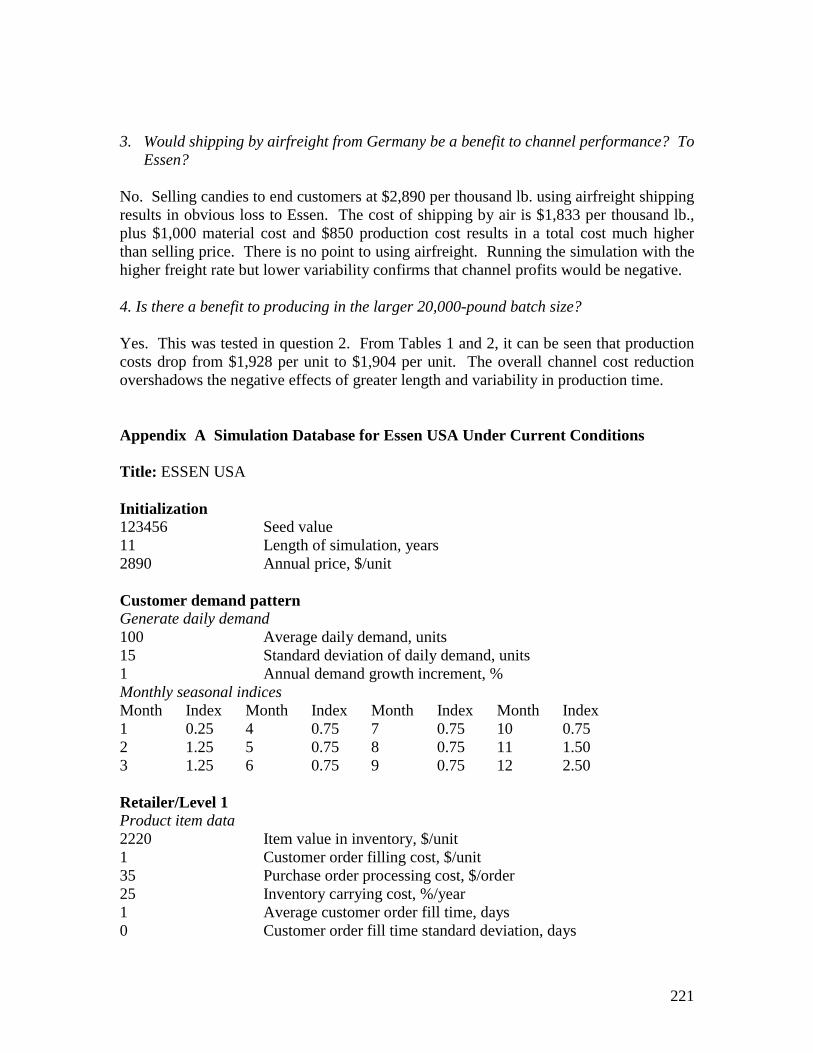
3. Would shipping by airfreight from Germany be a benefit to channel performance? To

Essen? No. Selling candies to end customers at $2,890 per thousand lb. using airfreight shipping results in obvious loss to Essen. The cost of shipping by air is $1,833 per thousand lb., plus $1,000 material cost and $850 production cost results in a total cost much higher than selling price. There is no point to using airfreight. Running the simulation with the higher freight rate but lower variability confirms that channel profits would be negative. 4. Is there a benefit to producing in the larger 20,000-pound batch size? Yes. This was tested in question 2. From Tables 1 and 2, it can be seen that production costs drop from $1,928 per unit to $1,904 per unit. The overall channel cost reduction overshadows the negative effects of greater length and variability in production time. Appendix A Simulation Database for Essen USA Under Current Conditions Title: ESSEN USA Initialization 123456 Seed value 11 Length of simulation, years 2890 Annual price, $/unit Customer demand pattern Generate daily demand 100 Average daily demand, units 15 Standard deviation of daily demand, units 1 Annual demand growth increment, % Monthly seasonal indices Month Index Month Index Month Index Month Index 1 0.25 4 0.75 7 0.75 10 0.75 2 1.25 5 0.75 8 0.75 11 1.50 3 1.25 6 0.75 9 0.75 12 2.50 Retailer/Level 1 Product item data 2220 Item value in inventory, $/unit 1 Customer order filling cost, $/unit 35 Purchase order processing cost, $/order 25 Inventory carrying cost, %/year 1 Average customer order fill time, days 0 Customer order fill time standard deviation, days

222

98 In-stock probability, % 670 Back order cost, $/unit Forecasting method Moving average 7 Number of periods Reorder policy Stock-to-demand control method 10 Target days of inventory 7 Review time in days Distributor/Level 2 Product item data 2220 Item value in inventory, $/unit 20 Retailer order filling cost, $/unit 75 Purchase order processing cost, $/order 25 Inventory carrying cost, %/year 2 Average retailer order fill time, days 0.2 Retailer order fill time standard deviation, days 95 In-stock probability, % 100 Back order cost, $/unit Forecasting method Moving average 30 Number of periods Reorder policy Stock-to-demand control method 45 Target days of inventory 30 Review time in days Warehouse/Level 3 Product item data 1710 Item value in inventory, $/unit 15 Distributor order filling cost, $/unit 75 Purchase order processing cost, $/order 20 Inventory carrying cost, %/year 3 Average distributor order filling time, days 0.3 Distributor order fill time, days 95 In-stock probability, % 25 Back order cost, $/unit Forecasting method Moving average 360 Number of periods Reorder policy Stock-to-demand control method 90 Target days of inventory 30 Review time in days

223

Factory/Source Product item data

850 Production cost, $/unit 10 Minimum production lot size, units 10 Warehouse order filling cost, $/unit 8 Average production time, days 2 Production time standard deviation, days 1000 Purchase cost, $/unit Transportation Transport between Distributor and Retailer

25 Transport cost, $/unit 1 Average time in-transit, days 0 Transit time standard deviation, days Transport between Warehouse and Distributor

70 Transport cost, $/unit 5 Average time in-transit, days 1 Transit time standard deviation, days Transport between Factory and Warehouse

78 Transport cost, $/unit 9 Average time in-transit, days 3 Transit time standard deviation, days Appendix B Benchmark Simulation Results with Seed Number 123456 and

Simulation Length of 11 Years SUPPLY CHANNEL REPORT FOR SIMULATED YEARS 2 TO 11

Yearly Simulatedaverage period FINANCIAL PERFORMANCE

$109,868,552 $1,098,685,520 Revenue37,918,000 379,180,000 Cost of purchased goods71,950,552 719,505,520 Gross margin

32,230,300 322,303,000 Production cost

Transportation costs:949,025 9,490,250 Distributor to retailer

2,656,010 26,560,100 Warehouse to distributor2,957,604 29,576,040 Factory to warehouse

Sales order handling cost for:38,017 380,168 Customer orders

759,890 7,598,900 Retailer orders569,145 5,691,450 Distributor orders

Order processing cost for:1,638 16,380 Orders to distributor

683 6,825 Orders to warehouses675 6,750 Orders to factory

Inventory costs

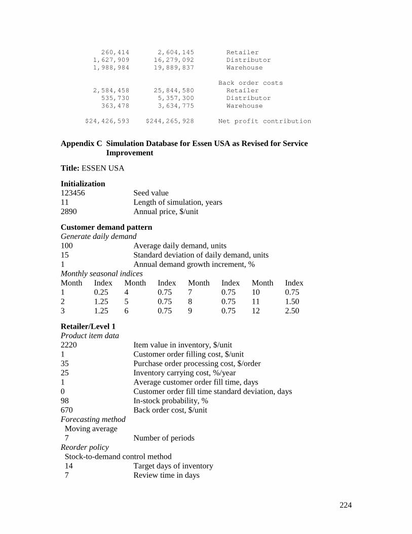
224

260,414 2,604,145 Retailer1,627,909 16,279,092 Distributor1,988,984 19,889,837 Warehouse

Back order costs2,584,458 25,844,580 Retailer

535,730 5,357,300 Distributor363,478 3,634,775 Warehouse

$24,426,593 $244,265,928 Net profit contribution

Appendix C Simulation Database for Essen USA as Revised for Service Improvement

Title: ESSEN USA Initialization 123456 Seed value 11 Length of simulation, years 2890 Annual price, $/unit Customer demand pattern Generate daily demand 100 Average daily demand, units 15 Standard deviation of daily demand, units 1 Annual demand growth increment, % Monthly seasonal indices Month Index Month Index Month Index Month Index 1 0.25 4 0.75 7 0.75 10 0.75 2 1.25 5 0.75 8 0.75 11 1.50 3 1.25 6 0.75 9 0.75 12 2.50 Retailer/Level 1 Product item data 2220 Item value in inventory, $/unit 1 Customer order filling cost, $/unit 35 Purchase order processing cost, $/order 25 Inventory carrying cost, %/year 1 Average customer order fill time, days 0 Customer order fill time standard deviation, days 98 In-stock probability, % 670 Back order cost, $/unit Forecasting method Moving average 7 Number of periods Reorder policy Stock-to-demand control method 14 Target days of inventory 7 Review time in days

225

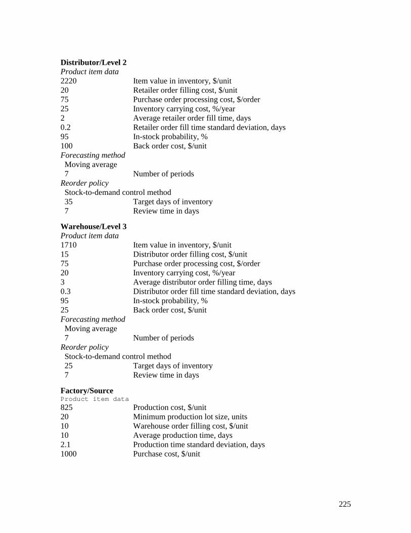
Distributor/Level 2 Product item data 2220 Item value in inventory, $/unit 20 Retailer order filling cost, $/unit 75 Purchase order processing cost, $/order 25 Inventory carrying cost, %/year 2 Average retailer order fill time, days 0.2 Retailer order fill time standard deviation, days 95 In-stock probability, % 100 Back order cost, $/unit Forecasting method Moving average 7 Number of periods Reorder policy Stock-to-demand control method 35 Target days of inventory 7 Review time in days Warehouse/Level 3 Product item data 1710 Item value in inventory, $/unit 15 Distributor order filling cost, $/unit 75 Purchase order processing cost, $/order 20 Inventory carrying cost, %/year 3 Average distributor order filling time, days 0.3 Distributor order fill time standard deviation, days 95 In-stock probability, % 25 Back order cost, $/unit Forecasting method Moving average 7 Number of periods Reorder policy Stock-to-demand control method 25 Target days of inventory 7 Review time in days

Factory/Source Product item data

825 Production cost, $/unit 20 Minimum production lot size, units 10 Warehouse order filling cost, $/unit 10 Average production time, days 2.1 Production time standard deviation, days 1000 Purchase cost, $/unit

226

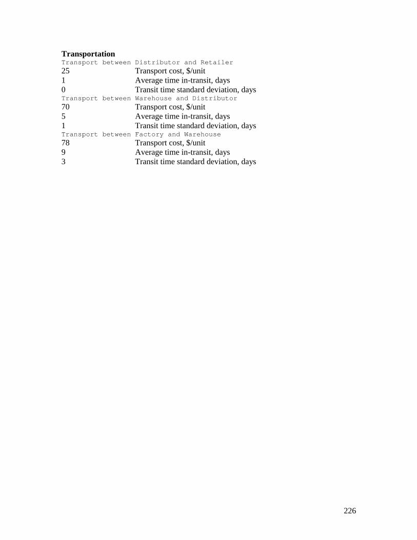
Transportation Transport between Distributor and Retailer

25 Transport cost, $/unit 1 Average time in-transit, days 0 Transit time standard deviation, days Transport between Warehouse and Distributor

70 Transport cost, $/unit 5 Average time in-transit, days 1 Transit time standard deviation, days Transport between Factory and Warehouse

78 Transport cost, $/unit 9 Average time in-transit, days 3 Transit time standard deviation, days