Baden-Württemberg Center of Applied Research Information ... · and its members, professors at universities of applied sciences in Baden-Württemberg, cover the whole area of communication

BW-CAR | SINCOM SYMPOSIUM ON INFORMATION

AND COMMUNICATION

SYSTEMS

3rd Baden-Württemberg Center of Applied Research

Symposium on

Information and Communication Systems

SInCom 2016

Karlsruhe, December 2nd, 2016

BW-CAR | SINCOMSYMPOSIUM ON INFORMATION AND COMMUNICATION SYSTEMS

Franz Quint, Dirk Benyoucef (Eds.)

ISBN: 978-3-943301-21-2

© Copyright 2016 Hochschule Offenburg Badstraße 24 77652 Offenburg [email protected] www.hs-offenburg.de

ii

Message from the Program Chairs

The Baden-Württemberg Center of Applied Research (BW-CAR) intends to further develop applied

research at the Universities of Applied Science (UAS). The BW-CAR working group Informations-

und Kommunikationssysteme (IKS) organizes in cooperation with the working group Technologien für

Intelligente Systeme (iTIS) the BW-CAR Symposium on Information and Communication Systems

(SInCom). This year it took place in its third edition at Karlsruhe University of Applied Sciences. IKS

and its members, professors at universities of applied sciences in Baden-Württemberg, cover the

whole area of communication and information systems. Retrieval, processing, transmission and

storage of information are key technologies in the digital age, with impact on all areas of modern life.

They are part of industry 4.0, mobile networks, smart grids, navigation systems, ambient assisted

living, environmental engineering, in macroscopic or in embedded systems such as smart phones and

sensor networks.

SInCom 2016 aimed at young researchers for contributions in the fields of

Algorithms for Signal and Image Processing

Communication Networks and Information Theory

Pattern Recognition

Control Theory

Distributed Computing

The program committee thanks all authors for their valuable contributions to SInCom 2016.

Furthermore, we express our great acknowledgment to the reviewers for their suggestions and help to

improve the papers. Finally, we appreciate very much the support of the rectorate and the help of many

employees of Karlsruhe University of Applied Sciences in organizing the symposium.

Karlsruhe, December 2nd, 2016

Franz Quint, Dirk Benyoucef

iii

iv

Organizing Committee

Prof. Dr. Franz Quint, Hochschule Karlsruhe

Prof. Dr. Dirk Benyoucef, Hochschule Furtwangen

Program Committee

Prof. Dr. Dirk Benyoucef, Hochschule Furtwangen

Prof. Dr.-Ing. Andreas Christ, Hochschule Offenburg

Prof. Dr. rer. nat. Thomas Eppler, Hochschule Albstadt-Sigmaringen

Prof. Dr. Matthias Franz, Hochschule Konstanz

Prof. Dr.-Ing. Jürgen Freudenberger, Hochschule Konstanz

Prof. Dr. Thomas Greiner, Hochschule Pforzheim

Prof. Dr. rer.nat. Roland Münzer, Hochschule Ulm

Prof. Dr.-Ing. Franz Quint, Hochschule Karlsruhe

Prof. Dr. Christoph Reich, Hochschule Furtwangen

Prof. Dr. Georg Umlauf, Hochschule Konstanz

Prof. Dr.-Ing. Axel Sikora, Hochschule Offenburg

Prof. Dr. Dirk Westhoff, Hochschule Offenburg

v

Content

Frequency Invariant Transformation of Periodic Signals (FIT-PS) for high frequency Signal Representation in NILM

Pirmin Held, Alaa Saleh, Djaffar Ould Abdeslam, Dirk Benyoucef 1

Chase decoding for quantized reliability information with applications to flash memories

Jürgen Freudenberger, Mohammed Rajab

Depth Estimation from Micro Images of a Plenoptic Camera

Jennifer Konz, Niclas Zeller, Franz Quint, Uwe Stilla 17

Feature Based RGB-D SLAM for a Plenoptic Camera

Andreas Kühefuß, Niclas Zeller, Franz Quint, Uwe Stilla 25

A Comparative Study of Data Clustering Algorithms

Ankita Agrawal, Artur Schmidt 31

A short survey on recent methods for cage computation

Pascal Laube, Georg Umlauf 37

Character Recognition in Satellite Images

Ankita Agrawal, Wolfgang Ertel 43

Towards Sensorless Control for Softlanding of Fast-Switching Electromagnetic Actuators

Tristan Braun, Johannes Reuter 49

Intelligent Fault Detection and Prognostics in Linear Electromagnetic Actuators – A Concept Description

Christian Knobel, Hanna Wenzl, Johannes Reuter 55

7

Martin Schall, Marc-Peter Schambach, Matthias O. Franz 11

Improving gradient-based LSTM training for offline handwriting recognition by careful selection of the optimization method

Secure Zero Configuration of IoT Devices - A Survey

Kevin Wallis, Christoph Reich 59

Frequency Invariant Transformation of Periodic

Signals (FIT-PS) for high frequency Signal

Representation in NILM

Pirmin Held1, Alaa Saleh1, Djaffar Ould Abdeslam2, and Dirk Benyoucef1

1Furtwangen University, Furtwangen, Germany

Email: {pirmin.held,alaa.saleh,dirk.benyoucef}@hs-furtwangen.de

2Universite de Haute-Alsace, Mulhouse, France

Email: [email protected]

Abstract—The aim of non-intrusive load monitoring is to de-termine the individual energy consumption of different devices onthe basis of the total energy consumption. The individual energyconsumption of a device is measured at a central point withoutthe need of individual measuring instruments on the devicesthemselves. In this work we present a signal representationfrequency invariant transformation of periodic signals (FIT-PS)[1] on high sampled signals.

We present a new method for signal separation, decompositionof the signal into individual states and feature extraction. Fre-quency invariant transformation of periodic signals (FIT-PS) isbased on a signal diagram similar to the concept of trajectories[2]–[4] utilizing the periodicity of voltage and current, and theircorrelation. This approach breaks down the current signal into itsindividual periods using the voltage as a reference signal for thedetermination of trigger points. Thereby, the phase informationbetween current and voltage is maintained and is inherentlypart of the new signal representation. In common approacheswith high sample rates several signal forms must be combinedto achieve good results. The advantage of this method is thatthe information contained in the signal is preserved entirely.Hence, this single signal representation is sufficient to createsimilar or even better results by using high sample rates. Theefficiency of the new signal representation and signal separationis demonstrated by the example of an event detection algorithm.For testing the BLUED dataset [5] was used reaching a sensitivityin event detection of 99.45%.

I. INTRODUCTION

The disaggregation of electrical energy consumption (non-

intrusive load monitoring (NILM)) determines the energy

consumption of individual electrical appliances from the total

energy consumption [6]. In NILM the quantities v(t) and i(t)are measured. They can be described as a function of the

amplitude V (t) or I(t) and the frequency f(t), respectively.

v(t) = V (t) · cos(2πf(t) · t+ ϕi(t)) (1)

i(t) = I(t) · cos(2πf(t) · t+ ϕv(t)) (2)

Equation (3) according to [7] describes the fundamental prob-

lem of modeling NILM.

y(t) =

D(t)∑

d=1

yd(t) for t = 1, ..., T (3)

y(t) ∈ R describes the sum of power consumption of several

devices d at a time t. Where yd(t) is the power consumption of

the device d at time t and D(t) is the number of devices in the

building. In general, neither the number of devices nor their

characteristics are known and thus a distinct solution does not

exist.

Most of the methods in literature use a linear process for

disaggregation which are described with the following four

steps: event detection, feature extraction, classification and

tracking [8]. The event detection determines the corresponding

switching points of the on and off times of the individual

devices. The knowledge of the switching points allows a

further distinction of the signal state: There are stationary

states zi, zi+1, . . . and between each two stationary states there

is a transient state.

In the early days of NILM [6] the differential power ∆P

and ∆Q are used. Nowadays there are numerous features like

harmonics, switching transient waveform, current waveform or

eigenvalues [10], [11]. This features can be distinguished in

steady state features and transient state features. While, steady

state features utilize the signal section before and after the

turning-on or switching-off procedure, transient state features

only make use of the signal sequence during the turning-on

or switching-off process. [12] proposes a procedure in which

both features are used in combination. The classification, or

distinction of different devices, is based on the results provided

by the event detection and the feature extraction [13]. Therefor,

each event which is not identified leads to a reduction of the

recognition rate and each false positive event represents an

error source for the classification.

The energy - tracking, which assigns the energy consumption

to the individual devices is the last step of the NILM.

An important question for a NILM system is the choice

of the sampling rate. In literature the sampling rate ranges

from a few Hz [6], [14]–[17] to several kHz [18], [19]. The

number of features that can be defined increases with a higher

sampling rate but also the calculation effort and the costs

for the whole system increase. The optimal feature for event

detection and classification depends on the kind and number

of devices, as well as on their switching behavior. In [10]

BW-CAR Symposium on Information and Communication Systems (SInCom) 2016

1

different combinations of features are used to produce better

results but it is hard to find a combination of features that suits

for all devices. The success of a NILM system depends highly

on the individual condition. Therefore, there is the possibility

to provide a variety of features in the hardware (HW) or to

customize the features by HW adjustment for the individual

equipment pool. In addition, the weighting of the features

should be adjusted depending on the application environment.

Frequency invariant transformation of periodic signals

(FIT-PS) is a new method of signal decomposition which

is independent of the main frequency and which results in

a signal representation without periodic oscillations. The

current is separated into its individual periods using the

voltage as a reference for the beginning of each period and

the determination of the subsequent sampling points in each

period.

In contrast to current waveform (CW) the voltage is used

as a trigger point for the determination of the periods.

Thereby, important information, such as active and reactive

power for example, remains. The decomposition results in

a multi-dimensional signal where all information, including

low and high frequencies, and the phase angle are preserved.

Furthermore, easy separation of steady states and transient

states is enabled.

The generated set of periods creates the feature space. Since

all information is preserved in this feature space, its solitary

application is sufficient. In this paper the versatility of the

introduced signal decomposition method is demonstrated at

the example of the event detection.

This paper is structured as follows: Section II introduces the

new signal representation FIT-PS. Section III presents an event

detection method which is optimized by using the new signal

representation. In section IV, the performance of an event

detection exploiting the new signal representation is shown.

The BLUED dataset [5] is used for the simulations. Addition-

ally, a measurement method is presented that functions without

converting data afterwards.

II. SIGNAL REPRESENTATION BY FIT-PS

This section describes the new feature space based on v(t)(1) and i(t) (2). First, the sampling resulting in the new signal

representation is described. Next, the structure of the new

signal representation will be explained. Since the frequency

of the power grid is not constantly 50 Hz or 60 Hz a mains

frequency invariant representation of the current signal is

necessary. This is realized using the permanently available

voltage signal.

FIT-PS splits the current signal i(t) into the individual

periods whereby the voltage signal v(t) is used as a synchro-

nization signal. This is shown in the first three plots of Fig.

1. Thus, the information of the phase angle between current

and voltage is preserved. This results in a nl×nk dimensional

feature space where nl is the number of periods and nk is the

number of sampling points in each period as it can be seen in

the last plot of Fig. 1.

2

4

6

8

10

12

14

16

18

20

22

24

26

28

30

32

34

36

38

40

samples

-2

-1

0

1

2

v /

V

a) Finding the zero crossings

2

4

6

8

10

12

14

16

18

20

22

24

26

28

30

32

34

36

38

40

42

samples

-2

-1

0

1

2

v /

V

b) Interpolation of the individual periods

2

4

6

8

10

12

14

16

18

20

22

24

26

28

30

32

34

36

38

40

42

samples

-2

-1

0

1

2

i /

A

c) Applying the indices of the voltage to the current

l (num

ber of periods)

2

d) Introducing additional dimension and sorting the signal periodically

-2

k samples / period

1

0

i /

A

1 2 3 4 5 6 7 8

2

9 10 11 12 13 14 15 16 17 18 19 20 21

Fig. 1. Graphic illustration of FIT-PS

The value of the signal i(t) is calculated by applying Eq.

(4). In Eq. (4) l numbers the periods of the signal i(t) and k

is the sample number within one period of the signal i(t).

N,N→ R

l, k 7→ i((l − 1) · Tg︸︷︷︸

period

+ Ts · k︸︷︷︸

inside one period

) (4)

Tg is the length of one period in seconds and Ts is the time

in seconds between two measurement points.

In Fig. 2 the FIT-PS representation of a i(t) is shown as a

colored surface. Here 600 periods are considered. Those 600periods contain two different steady states and a transient state.

Initially Fig. 2 shows the steady state zi of device 1. After the

300th period, device 2 is connected. Following an amplitude

change that is clearly apparent in all dimensions, the system

is in a transient state. Subsequently, the signal again reaches

a stationary state, the second steady state zi+1. Both steady

states have their minimum (k = 148) and their maximum


2

(k = 48) in the same dimension, but the waveform itself

has changed considerably from the steady state zi to zi+1.

At steady state zi, after the maximum in dimension k = 48,

the amplitude decreases quickly below zero (from the third

dimension on). Whereas at steady state zi+1, the value does

not reach a negative amplitude until the dimension k = 100.

The figure shows that the changes in each period l within a

steady state are very small.

Fig. 2. FIT-PS of a current signal. Steady state zi: device 1; Transient state:switching on procedure of device 2; Steady state zi+1: device 1 and 2

A. The influence of the sampling rate

In Fig. 3 the influence of different sampling rate is shown.

Each figure shows the same part of the signal, where a device

is switched on and transformed with FIT-PS, but with different

sampling frequencies. l is the number of periods and k is the

number of dimensions which change with different sampling

rates. With 1.5 kHz far fewer details can be seen. Due to the

low-pass characteristic during down sampling briefly occurring

peaks are smoothed. Therefore, the amplitude also changes

here, which can be seen particularly clearly at 1.5kHz.

III. EVENT DETECTION

We increase the sampling rate to 12 kHz (200 samples per

period), compared to [1] where a sampling rate of 1.2 kHz (20

samples per period) was used. Using FIT-PS allows a simple

method with low complexity for detecting switching events.

To reduce the influence of disturbances a low-pass filter (5)

is applied in each dimension k of the signal i(t). With the

low-pass filter (5) we get ITP (6)

hTP (l) =

M∑

g=0

bgδ[n− g] =

{

bn, 0 ≤ n ≤M

0, else(5)

ITP (l, k) =

(

hTP ∗ I

)(

l, k

)

∀ k (6)

where M is the length of the low-pass filter and bn are

the filter coefficients. Usually, in the NILM context multiple

devices need to be detected. This creates a large number of

combinatorial possibilities which are displayed in the feature

space. For this reason it is useful to consider only the derivative

Fig. 3. FIT-PS with different sampling rate

Eq. (9) and (10) in order to utilize the feature space more

effectively. The case that two devices change their state at

exactly the same time is excluded.

Using this event detection algorithm directly on higher

sample frequencies will produce significantly more false pos-

itives. The reason for this is device specific current peaks of

some devices. These current peaks occur only in individual

dimensions of the high-sampled signal marked with arrows in

Fig. 4. In the case of signals which were recorded at a lower

frequency (1.2 kHz), these peaks can not be seen because of

the more marked low-pass characteristic. To use FIT-PS with

higher sampling rates, the event detection algorithm has to be

modified.

Also because of the increased number of dimensions k


3

caused from the higher sample rate, a dimension reduction

using the principal component analysis (PCA) is included.

PCA gives the k-dimensional projection matrix (IPCA)l×k

where k << l.

IPCA = ITPW (7)

where W is a k by k matrix whose columns are the eigenvec-

tors of I⊤TP ITP .

Because there are obviously correlations between the single

dimensions (in ITP ) not all dimensions are needed after the

PCA. We are using only the first m loading vectors, so we get

only the first m principal components.

IPCAm = ITPWm (8)

This also reduces the problem of noise in some dimensions

as discussed in Fig. 4 and 5.

Fig. 4. current peaks at high sampled signal transformed with FIT-PS

Fig. 5. 3D view of current peaks at high sampled signal transformed withFIT-PS

In order to reduce the computational effort and to decrease

the complexity, the event detector uses a two-step process. In

the first stage each possible event is detected with a simple

threshold which is applied to the derivate of the signal. This

threshold is adjusted in order to detect all true positive (TP)

events. This leads to higher numbers of false positive (FP)

events. The signal ranges where potential events are identified

are examined more closely in the second stage. In the second

stage, the difference between the stationary level before and

after the event is calculated and compared with a second

threshold.

The derivative of IPCAm in direction of l is calculated using

Eq. (9) and (10). Φl shows the index where the derivative has

its maximum and is above the threshold Tr1.

L :=

{

l

∣

∣

∣

∣

∣

∣

∣

∣

∣

∂IPCAm(l,m)

∂l

∣

∣

∣

∣

≥ Tr1, ∀ k

}

(9)

Φl = argmaxk

∣

∣

∣

∣

∂IPCAm(l,m)

∂l

∣

∣

∣

∣

≥ Tr1 ∀ l ∈ L (10)

The advantage of using the maximum compared to the

average is that devices using a phase angle control can be

detected more efficiently because of the better signal-to-noise

ratio (SNR). These devices only use a part of the period

where the information is only conserved in a few dimensions.

The problem in event detection is the suppression of multiple

detections of the same event while maintaining the ability to

differentiate between events which are located very closely to

each other. Hence, a variable dead-time in which no additional

event is detected is introduced. The disadvantage of a dead-

time is that events which are too close to each other cannot

be recognized. In order to avoid losing events, the time range

in which no other event can be detected is set so that it starts

and terminates with the beginning and ending of each transient

state. For this purpose it is necessary to decompose the signal

into stationary and transient sections.

In Eq. (11) and (12) the start and end index, Φsl

and Φel ,

of the transient states are calculated with respect to a fixed

maximum length α. The distances Φl − Φsl and Φe

l − Φl,

respectively, depend on the specific devices.

Φsl = argmin

αVar(IPCAm(α,Φl)) (11)

with α = l, ...l +NA ∀ l ∈ L

Φel = argmin

αVar(IPCAm(α,Φl)) (12)

with α = l −NB , ...l ∀ l ∈ L

Where NA and NB are constants.

After determining the exact position of the transient section, a

second threshold Tr2 is used in (14) to reduce the number of

false positives. Here, the information of the steady state before

and after the detected event is used. As shown in (9) and (10)

a threshold is applied to the dimension with

τl =

Φs

l∑

n=Φs

l−(M−1)

IPCAm(n,Φl)

M

−

Φe

l+(M−1)∑

n=Φe

l

IPCAm(n,Φl)

M∀ l ∈ L (13)

over the mean of M values of the steady state before and after

the event. In equation (14) we get the final result, the indices

of the events E.

E = |τl| ≥ Tr2 ∀ l ∈ L (14)


4

1 2 3 4 5 6 7

number of used dimensions after PCA

75

80

85

90

95

100

recall

/ pre

cis

ion in %

recall phase 1

precision phase 1

recall phase 2

precision phase 2

Fig. 6. Comparison of the results of the event detection with different numbersof dimensions after PCA

IV. RESULTS

Applying the proposed feature space and the event detector

on the BLUED dataset, [5] allows a better comparability. In

difference to [1] where a sample frequency of 1.2 kHz was

used, a 12 kHz frequency was used for this work.

Due to the varying net frequency, measurement points also

have to vary during different periods. But for trajectories as

well as for our new approach constant points are required.

As first trigger point in a period, we decided to use the zero

crossing from negative to positive. The remaining 19 trigger

points were regularly distributed over this period. Signals

provided by the BLUED dataset [5] were used and converted

using voltage as reference.

Performance metrics (15) and (16) depend on TP, false

negative (FN) and FP and were used to receive a better

comparability.

Precall =TP

TP + FN(15)

Pprecision =TP

TP + FP(16)

Tab. I and II show the results of the event detection

based on FIT-PS (sample frequency of 1.2 kHz and 57 Hz)

in comparison to [20], where a modified generalize likelihood

ratio detector combined with a higher sampling rate was used.

The performance of all event detectors depends highly on each

phase considered.

TABLE IDETECTION PERFORMANCE BLUED PHASE A

BLUED (A) FIT-PS12 kHz PCA

FIT-PS1.2 kHz [1]

[20]

Precall 99.45% 99.31% 98.16%

Pprecision 98.15% 97.51% 97.94%

TABLE IIDETECTION PERFORMANCE BLUED PHASE B

BLUED (B) FIT-PS12 kHz PCA

FIT-PS1.2 kHz [1]

[20]

Precall 93.98% 87.37% 70.40%

Pprecision 83.50% 82.08% 87.29%

Concerning the sensitivity (Precall) FIT-PS with 12 kHz

at phase A leads to better results compared to the method

presented in [20] without significant loss of precision. In

contrast, the results of FIT-PS 1.2 Hz are slightly behind [20]

and FIT-PS with 12 kHz. The biggest advantage of FIT-PS

was shown when phase B was used. Even at the lower sample

rate, the sensitivity of FIT-PS outperforms the event detector

used in [20] significantly, with only minimal lower Pprecision

than [20]. Due to the dramatically reduced amount of data

and the subsequently difficult noise filtering, FIT-PS 1.2 kHz

shows reduced sensitivity and precision if compared to the

other FIT-PS.

Because a lot of electronic and appliances overlap at phase

B [5], the results for phase A were significantly better.

V. CONCLUSION

We present the frequency invariant transformation of peri-

odic signals FIT-PS for higher sample rates. We could show

that the use of higher sample rate entail better results.

The voltage is used as reference signal for the determination

of trigger points. With this information the current signal

is interpolated and fragmented into its individual periods.

Thereby the signal representation is independent from the

mains frequency. The entire information of the original signal

is retained.

Because of the highly increased number of dimensions (20

with 1.2 kHz to 200 with 12 kHz) the PCA is used to reduce

dimensions. Depending on the used thresholds Tr1 and Tr2 a

reduction to two or three dimensions leads to the best results.

The reason for this is the following event detection method.

Since the used event detection method is not complex enough

to completely take account of all available information, this

information has a disturbing effect on the event detector. PCA

reduces the number of information to an amount which can

be processed by the event detector.

For event detection this method was applied to the BLUED

dataset [5] resulting in a sensitivity of up to 99.45%.

In future, we plan to apply FIT-PS for a classification in

NILM. The issue of peaks in some dimensions caused by a

higher sampling rate for the event detector can thereby used

as additional feature.

This work was created as part of the iMon project (funding

number 03FH001IX4).


5

REFERENCES

[1] P. Held, F. Laasch, A. Djaffar Ould, and D. Benyoucef, “Frequencyinvariant transformation of periodic signals (FIT-PS) for signal represen-tation in NILM,” no. 42, accepted for publication but not yet published.

[2] L. Du, D. He, R. G. Harley, and T. G. Habetler, “Electricload classification by binary voltage–current trajectory mapping,”vol. 7, no. 1, pp. 358–365, 00000. [Online]. Available: http://ieeexplore.ieee.org/lpdocs/epic03/wrapper.htm?arnumber=7130652

[3] T. Guzel and E. Ustunel, “Principal components null space analysisbased non-intrusive load monitoring,” in Electrical Power and EnergyConference (EPEC), 2015 IEEE. IEEE, pp. 420–423, 00000. [Online].Available: http://ieeexplore.ieee.org/xpls/abs all.jsp?arnumber=7379987

[4] T. Hassan, F. Javed, and N. Arshad, “An empirical investigationof VI trajectory based load signatures for non-intrusive loadmonitoring,” vol. 5, no. 2, pp. 870–878, 00011. [Online]. Available:http://ieeexplore.ieee.org/xpls/abs all.jsp?arnumber=6575197

[5] K. Anderson, A. Ocneanu, D. Benitez, A. Rowe, and M. Berges,“BLUED: A fully labeled public dataset for event-based non-intrusiveload monitoring research,” in Proceedings of the 2nd KDD Workshopon Data Mining Applications in Sustainability (SustKDD).

[6] G. W. Hart, “Nonintrusive appliance load monitoring,” vol. 80, no. 12,pp. 1870–1891, 00954. [Online]. Available: http://ieeexplore.ieee.org/xpls/abs all.jsp?arnumber=192069

[7] R. Dong, L. Ratliff, H. Ohlsson, and S. S. Sastry, “Fundamental limitsof nonintrusive load monitoring,” in Proceedings of the 3rd internationalconference on High confidence networked systems. ACM, pp. 11–18,00014. [Online]. Available: http://dl.acm.org/citation.cfm?id=2566471

[8] L. Jiang, S. Luo, and J. Li, “Automatic power load event detectionand appliance classification based on power harmonic features innonintrusive appliance load monitoring,” in Industrial Electronics andApplications (ICIEA), 2013 8th IEEE Conference on. IEEE, pp.1083–1088, 00004. [Online]. Available: http://ieeexplore.ieee.org/xpls/abs all.jsp?arnumber=6566528

[9] B. Wild, K. S. Barsim, and B. Yang, “A new unsupervised eventdetector for non-intrusive load monitoring,” in 2015 IEEE GlobalConference on Signal and Information Processing (GlobalSIP). IEEE,pp. 73–77, 00000. [Online]. Available: http://ieeexplore.ieee.org/xpls/abs all.jsp?arnumber=7418159

[10] J. Liang, S. K. K. Ng, G. Kendall, and J. W. M. Cheng, “Load signaturestudy—part II: Disaggregation framework, simulation, and applications,”vol. 25, no. 2, pp. 561–569, 00083. [Online]. Available: http://ieeexplore.ieee.org/lpdocs/epic03/wrapper.htm?arnumber=5337970

[11] ——, “Load signature study—part i: Basic concept, structure,and methodology,” vol. 25, no. 2, pp. 551–560, 00195.[Online]. Available: http://ieeexplore.ieee.org/lpdocs/epic03/wrapper.htm?arnumber=5337912

[12] H.-H. Chang, C.-L. Lin, and J.-K. Lee, “Load identification innonintrusive load monitoring using steady-state and turn-on transientenergy algorithms,” in Computer supported cooperative work in design(cscwd), 2010 14th international conference on. IEEE, pp. 27–32,00050. [Online]. Available: http://ieeexplore.ieee.org/xpls/abs all.jsp?arnumber=5472008

[13] Y. F. Wong, Y. Ahmet Sekercioglu, T. Drummond, and V. S. Wong,“Recent approaches to non-intrusive load monitoring techniques inresidential settings,” in Computational Intelligence Applications InSmart Grid (CIASG), 2013 IEEE Symposium on. IEEE, pp. 73–79,00012. [Online]. Available: http://ieeexplore.ieee.org/xpls/abs all.jsp?arnumber=6611501

[14] Z. Zhang, J. H. Son, Y. Li, M. Trayer, Z. Pi, D. Y. Hwang,and J. K. Moon, “Training-free non-intrusive load monitoring ofelectric vehicle charging with low sampling rate,” in IndustrialElectronics Society, IECON 2014-40th Annual Conference of theIEEE. IEEE, pp. 5419–5425, 00004. [Online]. Available: http://ieeexplore.ieee.org/xpls/abs all.jsp?arnumber=7049328

[15] S. Barker, A. Mishra, D. Irwin, E. Cecchet, P. Shenoy, and J. Albrecht,“Smart*: An open data set and tools for enabling research in sustainablehomes,” vol. 111, p. 112, 00000. [Online]. Available: http://wan.poly.edu/KDD2012/forms/workshop/SustKDD12/doc/SustKDD12 3.pdf

[16] L. Mauch and B. Yang, “A new approach for supervised powerdisaggregation by using a deep recurrent LSTM network,” in 2015IEEE Global Conference on Signal and Information Processing(GlobalSIP). IEEE, pp. 63–67, 00000. [Online]. Available: http://ieeexplore.ieee.org/xpls/abs all.jsp?arnumber=7418157

[17] J. Liao, G. Elafoudi, L. Stankovic, and V. Stankovic, “Non-intrusiveappliance load monitoring using low-resolution smart meter data,”in Smart Grid Communications (SmartGridComm), 2014 IEEEInternational Conference on. IEEE, pp. 535–540, 00011. [Online].Available: http://ieeexplore.ieee.org/xpls/abs all.jsp?arnumber=7007702

[18] C. Duarte, P. Delmar, K. Barner, and K. Goossen, “A signal acquisitionsystem for non-intrusive load monitoring of residential electrical loadsbased on switching transient voltages,” in Power Systems Conference(PSC), 2015 Clemson University. IEEE, pp. 1–6, 00001. [Online].Available: http://ieeexplore.ieee.org/xpls/abs all.jsp?arnumber=7101707

[19] R. Jonetzko, M. Detzler, K.-U. Gollmer, A. Guldner, M. Huber,R. Michels, and S. Naumann, “High frequency non-intrusive electricdevice detection and diagnosis,” in Smart Cities and Green ICTSystems (SMARTGREENS), 2015 International Conference on. IEEE,pp. 1–8, 00001. [Online]. Available: http://ieeexplore.ieee.org/xpls/absall.jsp?arnumber=7297979

[20] K. D. Anderson, M. E. Berges, A. Ocneanu, D. Benitez, andJ. M. Moura, “Event detection for non intrusive load monitoring,” inIECON 2012-38th Annual Conference on IEEE Industrial ElectronicsSociety. IEEE, pp. 3312–3317, 00032. [Online]. Available: http://ieeexplore.ieee.org/xpls/abs all.jsp?arnumber=6389367


6

Chase decoding for quantized reliability information

with applications to flash memories

Jurgen Freudenberger, Mohammed Rajab

Institute for System Dynamics

HTWG Konstanz, University of Applied Sciences, Germany

Email: {jfreuden,mrajab}@htwg-konstanz.de

Web: www.isd.htwg-konstanz.de

Abstract—Chase decoding is an established soft-input decoding

method for algebraic error correcting codes. This paper analyses

the performance of Chase type II decoding using quantized

input data, where transmission of binary data over the additive

white Gaussian noise (AWGN) channel is assumed. The channel

output symbols are quantized with a small number of decision

thresholds. This channel model is applicable for data storage

in flash memories. Simulation results demonstrate that the soft

decoding performance of the Chase algorithm can be improved

by optimizing the threshold values for the quantization.

I. INTRODUCTION

Flash memories are becoming more and more important for

non-volatile mass storages, where a flash memory stores the

information in floating gates which can be charged and erased.

These floating gates keep their electrical charge without a

power supply. However, information may be read erroneously.

The error probability depends on the storage density. The

NAND Flash used different type of levels as single-level-cell

(SLC), and currently the devices used multiple levels and are

mentioned to as multiple-level cell (MLC) flash or triple-level

cell (TLC) and on the number of program and write cycles [1].

In flash memories, error correction coding (ECC) is required

in order to ensure integrity and reliability [2], [3]. Soft-input

decoding can improve the error correcting capability compared

to hard-input decoding, where the soft-input decoding is based

on reliability information from the channel [4], [5]. To obtain

reliability information the medium must be read several times

using different read threshold voltages. Typically only a small

number of reads is used resulting in reliability information

with coarse quantization.

Chase decoding algorithms are reliability based decoding

procedures that generate a list of candidate codeword by

flipping bits in the received word [6], [7]. The test patterns

for the bit flipping are based on the least reliable positions of

the received word. For each test pattern, algebraic hard-input

decoding is employed. Finally, the best candidate from the list

is obtained by minimizing the Euclidean distance between the

candidate codewords and the received word. Chase devised

three different algorithms. The main difference between the

algorithms is the number of test patterns. The complexity of

Chase decoding depends on the size of the list of the candi-

dates. In this paper, we investigated Chase type II decoding for

quantized reliability information. In particular, we optimize the

read threshold in order to improve the decoding performance

with quantized reliability information.

This paper is structured as follows. Section II introduces the

threshold voltage of flash memories and the channel model.

In Section III the Chase decoding algorithm is described.

Simulation results are presented in Section IV.

II. THRESHOLD VALUES

With flash memories, the cells are addressed with so-called

word-lines, where a threshold voltage is required to turn on

a particular transistor. The value of the threshold voltage

varies from cell to cell. The probability density function of

the variation of threshold voltages is usually modelled by a

Gaussian distribution. Hence, the channel model for flash cells

is equivalent to an additive white Gaussian noise (AWGN)

channel. However, in order to obtain reliability information

for the channel input values, multiple reads with different

threshold values are required. The reading procedure for relia-

bility information causes additional latency. Thus, only a small

number of thresholds are applied in practice. Assuming i.i.d.

Gaussian threshold voltages, the channel of a flash memory

with reliability information can be considered as an AWGN

channel with quantized channels values.

In the following, we assume a reading procedure with five

threshold voltages. Fig. 1 shows the probability distribution of

the threshold values, where the reading threshold voltages are

denoted by δ1 and δ2. Hence, for the area between 0 and −δ1or −δ1 corresponds to the most unreliable input values. We

assume that the flash channel can be modelled as quantized

AWGN channel with the following quantization function

ri =

1 , ri > δ2δ2 , δ1 < ri ≤ δ2δ1 , 0 ≤ ri ≤ δ1−δ1 , 0 > ri ≥ −δ1−δ2 ,−δ1 > ri ≥ −δ2−1 , ri < −δ2

(1)

where ri denotes the i-th channel value and ri the correspond-

ing quantized channel value. In this work, we optimize the

values δ1 and δ2 for Chase decoding.


7

+δ1 +δ2−δ1−δ2

−2 −1 0 1 2ri

pro

bab

ilit

yden

sity

p(r

i)

Fig. 1. Probability density function with reading thresholds δ1 and δ2.

III. CHASE DECODING ALGORITHM

The Chase algorithm is a multi-trial procedure where bit

flipping is applied to the least reliable received values. Then

algebraic decoding is applied to determine a valid codeword.

Using different test patterns for the bit flipping, a list of

candidate codewords is obtained. Finally, the most likely

codeword is selected from this list. For the AWGN channel,

the most likely codeword can be determined by minimizing

the Euclidean distance between the received word and the

codewords in the list of candidates. With Chase type II

decoding a list of 2m candidates is obtained by systematically

testing all combinations of the m least reliable positions within

the received codeword. Typically, the parameter m is chosen

as m = dmin

2, where dmin is the minimum Hamming distance

of the code. Note that Chase type II decoding is a suboptimal

decoding procedure, because the maximum likelihood code-

word is not always in the list of candidates obtained by bit

flipping.

With Chase decoding, typically unquantized channel values

are assumed. In this work, we investigate Chase decoding with

quantized channel values. Note that with quantized channel

inputs, the set of the dmin

2least reliable positions is not always

unique. Moreover, minimization of the Euclidean distance

among the list of candidates does not always result in a

unique solution. We propose some modifications to the Chase

algorithms taking the quantization into consideration.

We consider binary codes of length n. The received se-

quence is denoted by r = (r1, r2, ..., rn). z = (z1, z2, ..., zn)is the binary hard-decision sequence corresponding to the

received sequence r. If z is a valid codeword, then it is the

the maximum likelihood codeword [5]. Thus, we calculate the

syndrome value for z and apply the Chase decoding only for

non-zero syndrome values as shown in Fig. 2. Moreover, we

choose m = dmin

2+1, because the set of the dmin

2least reliable

positions can not always be determined uniquely.

Finally, we propose a decoding procedure that may declare a

decoding failure. With quantized input values, Chase decoding

does not always result in a unique codeword, i.e., there might

be two or more codewords in the list of candidates which

have the same Euclidean distance to the received word. In this

case, the probability of a decoding error is high, because the

probability of selecting the correct codeword is at most a half.

If the decoding procedure is used in a concatenated coding

scheme, the decoder may declare a failure. Such a decoding

failure can be exploited using error and erasure decoding in

the next decoding stage.

Received word

Syndrome checkingz

Syndrome=0 Syndrome6= 0

Chase II decoding

c

r

Fig. 2. Flow chart of the decoding process

IV. SIMULATION RESULT

In this section, we present simulation results that demon-

strate the influence of the quantization on the decoding perfor-

mance. All simulations are based on a binary Bose-Chaudhuri-

Hocquenghem (BCH) code of length n = 118 and minimum

Hamming distance dmin = 4. Hence, we choose m = 3.

This code can be used as inner code in a concatenated code

as proposed in [5], [8]. The first simulation results consider

transmission over the AWGN channel without quantization.

We compare the performance of Chase type II and III decoding

with algebraic hard-input decoding.

In Fig. 3, Chase II has the lowest word error rate (WER)

compared with Chase III and hard-input decoding. Chase

II shows approximately 0.5 dB and 1.2 dB gain compared

with Chase III and hard-input decoding, respectively. For the

considered code, Chase II is twice as complex as Chase III,

i.e., type II decoding considers 8 test patterns and type III only

4.

A. Threshold values

In the following, we consider simulations with quantization.

In communication systems, typically linear quantization is

used where the values of the quantization thresholds are

uniformly spaced. If B = 3 bits represent the amplitude of

a sample, linear quantization results in the threshold values

δ1 = 0.25 and δ2 = 0.5 for the smallest quantization

thresholds. However, these values to not lead to the best

possible decoding performance. We demonstrate this in Fig. 4,

where we choose δ2 = 0.5 and vary the value of δ1. Fig. 4

shows that the decoding performance heavily depends on the


8

SNR [dB]

4 4.5 5 5.5 6 6.5

WE

R

10-4

10-3

10-2

10-1

100

Hard input

Chase II

Chase III

Fig. 3. A comparison between Chase II, Chase III, and hard-input decodingfor the AWGN channel without quantization.

threshold values, where the best performance is obtained with

δ1 = 0.2.

SNR [dB]

4 4.5 5 5.5 6 6.5

WE

R

10-4

10-3

10-2

10-1

100

BLER δ1= 0.05, δ

2= 0.50

BLER δ1= 0.10, δ

2= 0.50

BLER δ1= 0.15, δ

2= 0.50

BLER δ1= 0.20, δ

2= 0.50

BLER δ1= 0.25, δ

2= 0.50

Fig. 4. A comparison of different values of δ1 for a fixed value of δ2 = 0.5.

In Fig 4, the values δ1 = 0.15 and 0.2 result in a similar

performance with an average gain of 0.5dB compared with

δ1 = 0.05. In order to optimize both threshold values, we

choose δ1 in the interval from 0.1 to 0.2 and vary the second

threshold δ2, where the best results are obtained for δ1 = 0.15.

In Fig. 5, the second threshold value δ2 is adjusted based

on δ1 = 0.15. The dependency of the decoding performance

on δ2 is smaller than on δ1. For low SNR values the curves

are close to each other. The value δ2 = 0.4 is chosen for the

second threshold.

Fig. 6 shows results for a fixed δ2 = 0.4 and different values

of δ1. The thresholds δ1 = 0.15 results in the best performance

SNR [dB]

4 4.5 5 5.5 6 6.5

WE

R

10-4

10-3

10-2

10-1

100

BLER δ1= 0.15, δ

2= 0.35

BLER δ1= 0.15, δ

2= 0.40

BLER δ1= 0.15, δ

2= 0.45

Fig. 5. A comparison for different values of the second threshold δ2 and afixed value of δ1 = 0.15

SNR [dB]

4 4.5 5 5.5 6 6.5

WE

R

10-4

10-3

10-2

10-1

100

BLER δ1= 0.10, δ

2= 0.40

BLER δ1= 0.15, δ

2= 0.40

BLER δ1= 0.20, δ

2= 0.40

Fig. 6. A Comparison between different values of first threshold δ1 with afixed value of δ2= 0.4

for the complete range of SNR values, where the differences

are very small for high SNR values.

Finally, we consider a comparison of the performance

with quantized versus unquantized reliability information. The

corresponding simulation results are plotted in Fig. 7. The per-

formance degradation with quantized input with the optimized

threshold values is very small. For high SNR values the loss

is less than 0.1dB.

B. Decoding failure declaration

Next we consider the performance of the failure declaring

decoder. The quantization values of δ1 and δ2 are 0.15 and

0.4, respectively for this simulation. With this simulations,

the decoder declares a failure when the choice of the best


9

4 4.5 5 5.5 6 6.5

SNR [dB]

10-4

10-3

10-2

10-1

100

WE

R

Hard input

Chase II without quantization

Chase II with quantization

Fig. 7. Performance of Chase II decoding algorithm with quantized andunquantized inputs.

candidate is not unique. In this case, we have to error events:

a decoding failure and a decoding error (word error). In a

concatenated scheme, failures can be exploit using algebraic

errors and erasures decoding procedures. For instance, a de-

coder for Reed-Solomon codes that can correct t errors can

correct up to 2t erasures.

SNR [dB]

4 4.5 5 5.5 6 6.5

WE

R

10-4

10-3

10-2

10-1

100

BLER without Erasure,δ1= 0.15, δ

2= 0.40

BLER with Erasure, δ1= 0.15, δ

2= 0.40

Erasure, δ1= 0.15, δ

2= 0.40

Fig. 8. Performance of Chase II algorithm with and without code blockerasure.

In Fig. 8 it can be seen that the WER with erasure decoding

is lower than the WER of the same code without erasure

decoding. The decoding failure declaration shows an average

gain of 0.3dB compared with decoding without decoding

failure declaration.

V. CONCLUSION

In this paper we have investigated Chase II decoding with

quantized input. The simulation results demonstrate that the

performance loss due to quantization can be reduced by a

suitable choice of threshold values. This optimization has

applications to NAND flash memories, where reliability infor-

mation is obtained by a multiple-read procedure with different

threshold voltages.

With quantized input values, Chase decoding does not

always result in a unique codeword. In this case, the decoder

may declare a failure, because the probability of a decoding

error is high. In a concatenated coding scheme, such decoding

failures can be exploited using error and erasure decoding. The

presented simulation results shown that the decoding failure

declaration can improve the error and erasure performance.

ACKNOWLEDGMENT

We thank Hyperstone GmbH, Konstanz for supporting

this project. The German Federal Ministry of Research and

Education (BMBF) supported the research for this article

(03FH025IX5).

REFERENCES

[1] R. Micheloni, A. Marelli, and R. Ravasio, Error Correction Codes forNon-Volatile Memories. Springer, 2008.

[2] E. Yaakobi, J. Ma, L. Grupp, P. Siegel, S. Swanson, and J. Wolf,“Error characterization and coding schemes for flash memories,” in IEEEGLOBECOM Workshops, Dec. 2010, pp. 1856–1860.

[3] J. Freudenberger and J. Spinner, “A configurable Bose-Chaudhuri-Hocquenghem codec architecture for flash controller applications,” Jour-nal of Circuits, Systems, and Computers, vol. 23, no. 2, pp. 1–15, Feb2014.

[4] G. Dong, N. Xie, and T. Zhang, “On the use of soft-decision error-correction codes in NAND Flash memory,” IEEE Transactions on Circuitsand Systems I: Regular Papers, vol. 58, no. 2, pp. 429–439, Feb 2011.

[5] J. Spinner, J. Freudenberger, and S. Shavgulidze, “A soft input decodingalgorithm for generalized concatenated codes,” IEEE Transactions onCommunications, vol. 64, no. 9, pp. 3585–3595, Sept 2016.

[6] D. Chase, “Class of algorithms for decoding block codes with channelmeasurement information,” IEEE Transactions on Information Theory,pp. 170–182, 1972.

[7] M. P. Fossorier and S. Lin, “Chase-type and GMD coset decodings,” IEEETransactions on Communications, vol. 48, no. 3, pp. 345–350, 2000.

[8] J. Spinner, M. Rajab, and J. Freudenberger, “Construction of high-rategeneralized concatenated codes for applications in non-volatile flashmemories,” in 2016 IEEE 8th International Memory Workshop (IMW),May 2016, pp. 1–4.


10

Improving gradient-based LSTM training for o�inehandwriting recognition by careful selection of the

optimization method

Martin SchallInstitute for Optical SystemsUniversity of Applied Sciences

Constance, GermanyEmail: [email protected]

Marc-Peter SchambachSiemens Postal, Parcel &Airport Logistics GmbHConstance, Germany


Matthias O. FranzInstitute for Optical SystemsUniversity of Applied Sciences

Constance, GermanyEmail: [email protected]

Abstract—Recent years have seen the proposal of severaldi�erent gradient-based optimization methods for trainingarti�cial neural networks. Traditional methods include steep-est descent with momentum, newer methods are based onper-parameter learning rates and some approximate Newton-step updates. This work contains the result of several experi-ments comparing di�erent optimization methods. The exper-iments were targeted at o�line handwriting recognition usinghierarchical subsampling networks with recurrent LSTMlayers. We present an overview of the used optimizationmethods, the results that were achieved and a discussion ofwhy the methods lead to di�erent results.

Index Terms—o�line handwriting recognition; recurrentneural network; long-short-term-memory; connectionist tem-poral classi�cation; gradient-based learning; adadelta; rm-sprop

I. Introduction

Advances in the �eld of unconstrained and segmentation-free o�ine handwriting recognition using arti�cial neuralnetworks have been considerable in the last years [1] andcomplete systems for this task have been published [2].O�ine handwriting recognition is in use in applicationssuch as postal automation, banking and historical documentanalysis.

State of the art solutions for Latin script o�ine handwrit-ing recognition are based on Multi-Dimensional Long-Short-Term-Memory MDLSTM [3] [4] recurrent neural networksorganized as hierarchical subsampling networks [5]. Suchnetworks can be trained for sequence classi�cation usingConnectionist Temporal Classi�cation CTC [6]. CTC allowsthe training of networks for segmentation-free sequence clas-si�cation without knowledge about the location of containedlabels, based only on knowledge about the correct labelsequence.

Newton’s method can be used to determine an individualstep-size for each parameter during backpropagation trainingof the arti�cial neural network [7]. Using Newton’s methodleads to fast convergence rates but requires the calculationof second-order derivatives of the error function. Since thecalculation of second-order information is computationallyexpensive during backpropagation-based training, methods

like AdaDelta [8] try to approximate it using only �rst-orderinformation.

RProp [9] [10] provides an individual learning rate perparameter using only the changes in the sign of the partialderivative, similar to the Manhattan rule. RMSProp [11] im-proves on this concept by generalizing to mini-batch trainingvariants of the backpropagation algorithm. RMSProp does soby normalizing the gradient using the rolling mean value ofthe previous �rst-order derivatives.

This work provides an overview and comparison of con-temporary gradient-based optimization methods for traininghierarchical subsampling MDLSTM-networks using CTC. Allexperiments were done using the IAM o�ine handwritingdatabase [12]. It is meant as a guide for practitioners in the�eld of o�ine handwriting recognition. In addition, this workincludes theoretical interpretations of the observed results.

The paper starts by describing the used network topologyin section II, the investigated optimization methods in sectionIII and the experiments executed in section IV. Section Vpresents the results of the experiments and section VI dis-cusses the problems arising with the optimization methods.Section VII concludes the paper.

II. Network

The network topology was identical for all experimentsand is based on the hierarchical subsampling network usingMDLSTM-cells applied for Arabic handwriting recognition[2] [5]. While the network topology was unchanged, the hy-perparameters and sizes of the neuron layers were modi�ed.The exact network topology, beginning at the network input,and hyperparameters are described in table I.

The LSTM variant [13] used in the comparisons includesforget gates, peephole connections, bias values and the fullgradient for backpropagation. The fully connected feedfor-ward neurons had no bias, except for the very last neuronlayer. The non-linearities are the standard logistic sigmoidφ(x) = 1

1+e−x for the LSTM gates and the hyperbolic tangenttanh(x) for all other activations. The network consists ofa total of 148799 parameters, all of which were initialized


11

TABLE INetwork topology used for the experiments

Type of layer Con�gurationInput image Grayscale; 81 pixel in heightSubsampling 2× 3 (width × height)MDLSTM 2 cells per scan directionSubsampling 2× 3 (width × height)Fully connected feedforward 6 neurons; no biasMDLSTM 10 cells per scan directionSubsampling 2× 3 (width × height)Fully connected feedforward 20 neurons; no biasMDLSTM 50 cells per scan directionFully connected feedforward 79 neurons; with biasCollapseSoftmaxCTC 78 glyph labels; 1 blank label

drawing from a random uniform distribution in the interval[−0.1;+0.1].

III. Methods

The following paragraphs outline the gradient-based op-timization methods: Steepest descent with momentum, RM-SProp and AdaDelta. In all equations, gt is the gradient attime t and δxt the parameter updates at time t. µ is alwaysthe learning rate, α the decay rate and β the dampeningfactor. All variables are initialized to zero if not otherwisede�ned.

Algorithm 1 Steepest descent with momentum

δxt = (µ× gt) + (α× δxt−1)

Algorithm 1 describes the steepest descent optimizer witha simple momentum term added. It scales the �rst-orderderivative of the error function by a constant learningrate, thus generating parameter updates that are directlyproportional to the gradient. The added momentum termprevents the optimizer from following jitters in the errorfunction along the current path. Figuratively speaking, ifthe optimization process is a ball moving down the errorlandscape, momentum changes the gradient from being avector of movement to a vector of force applied to the ball.

Algorithm 2 RMSProp

E[g2]t = ((1− α)× g2t ) + (α× E[g2]t−1)δxt = µ× gt√

E[g2]t

RMSProp, outlined in Algorithm 2, is a generalization ofRProp that allows mini-batch training. Both only take thesign of the gradient into account but determine the step sizeof parameter updates independently from the absolute valueof the gradient. RMSProp does so by using a rolling meanof the gradient for normalization. It e�ectively allows theuser to choose the actual step size of parameter updates asa hyperparameter.

Algorithm 3 describes AdaDelta, which uses an approxima-tion of the diagonal values of the Hessian matrix to do quasi-

Algorithm 3 AdaDelta with additional learning rate

E[g2]t = ((1− α)× g2t ) + (α× E[g2]t−1)

ut = gt ×

√E[δx2]t−1+β√E[g2]t+β

E[δx2]t = ((1− α)× u2

t ) + (α× E[δx2]t−1)δxt = µ× ut

Newton updates. AdaDelta provides per-dimension step sizesand basically removes the need to manually choose a learningrate. The idea behind AdaDelta is outlined in the accordingpublication [8], calculating the parameter updates based onthe inverse Hessian as δx

g. Since both the total parameter

updates δx and the total gradient g for the Newton step areunknown, they are approximated using a rolling mean of thelast values. A variant of AdaDelta adds an additional learningrate µ, which should be chosen as a value near 1.0 since theunmodi�ed AdaDelta implies a global learning rate of 1.0.When gradient clipping was applied, only the error signal

that is transported from a LSTM layer to its predecessorwas truncated. Recalling the network topology de�ned inTable I, this concerns only the transition between the lasttwo MDLSTM layers and their previous fully connectedfeedforward layers. The error signal was hard clipped to bewithin the interval [−1;+1].

IV. Experiments

All experiments were carried out using the IAM o�inehandwriting database [12] with the images being rescaled to8-bit grayscale and �xed 81 pixel in height with a variablewidth. A random subset of 90% (86809) samples were usedfor training and 5% (4822) each for validation and evaluation.A sample of the IAM database is shown in �gure 1.

Fig. 1. Example of the IAM database

The network is speci�ed in section II and the targetfunction of supervised training was CTC with 78 visiblecharacter classes of the IAM database. No normalization oflabels was applied.If not otherwise noted, the training was done using mini-

batch updates of size 8 and the full non-clipped gradient.The gradients within a mini-batch were summed, but notnormalized afterwards. The training samples were processedin a random permutation for each training epoch. Theexperiments used early stopping until the validation errorrate did not improve for 5 epochs.The following individual experiments were conducted in

this work:

1) Steepest descent with momentum and full gradient.2) Steepest descent with momentum and gradient clip-

ping.


12

3) RMSProp.4) AdaDelta without additional learning rate.5) AdaDelta with additional learning rate.

The hyperparameters were chosen on basis of previousexperiments with this network architecture and the IAMdatabase. The hyperparameters have proven to be suitablefor training this network for o�ine handwriting recognition.

Error rate was measured in terms of Character Error RateCER at the end of each training epoch. CER is de�ned as

the percentage CER(y, z) = 100×ED(y,z)

|y| . It measures the

part of the edit-distance [14] ED(y, z) between the correctlabel string y and the decoded network output z in relationto the length |y| of the correct label. The CER of theseexperiments are averages over all samples within the trainingset or validation set respectively.

V. Results

Fig. 2. Steepest descent with µ = 1e−4 and α = 0.9

Fig. 3. Steepest descent with µ = 1e−4 and α = 0.9 (gradient clipping)

Figures 2 and 3 show the convergence of the CER duringtraining using steepest descent with momentum. Hyperpa-rameters were µ = 1e−4 and α = 0.9. The training usingthe full non-clipped training did not converge to acceptableerror rates as can be seen in �gure 2. The use of gradientclipping did improve the convergence of CER, see �gure 3,

during training. The convergence rate is still lower than withRMSProp or AdaDelta, however.As can be seen in �gure 2, the CER initially decreases for

some epochs but then started increasing again and stabilizesat 99%.

Fig. 4. RMSProp with µ = 1e−3 and α = 0.9

Figure 4 shows the convergence of the error rate usingRMSProp with µ = 1e−3 and α = 0.9. It shows a fasterconvergence rate than steepest descent with gradient clippingand achieves a lower error rate.

Fig. 5. AdaDelta with µ = 1, α = 0.95 and β = 1e−6

Fig. 6. AdaDelta with µ = 0.5, α = 0.95 and β = 1e−6


13

Figures 5 and 6 contain the results using AdaDelta. Bothuse the hyperparameters α = 0.95 and β = 1e−6. Theexperiment described in �gure 5 used a learning rate ofµ = 1, thus corresponds to the original work by the authorsof AdaDelta [8]. Figure 6 uses an additional learning rate ofµ = 0.5, which reduces the convergence rate by the samefactor. Using an additional learning rate proved to result inlower �nal error rates.

The fastest convergence rate in these experiments wasachieved using AdaDelta with µ = 1, α = 0.95 andβ = 1e−6, the lowest error rate with AdaDelta and µ = 0.5.

VI. Discussion

Fig. 7. Exemplary saddle point of an error function in a two-dimensionalparameter space

In the following section, we discuss possible reasons forwhy the compared optimization methods behave di�erentlyin terms of convergence of network error. Recent work [15][16] has shown that saddle points in the error functiontend to be a major problem while training arti�cial neuralnetworks. Other potential problems arise from the interactionbetween Backpropagation-Through-Time BPTT [17] and amomentum term in the optimization method. Figure 7 showsan error function with a saddle point that highlights thedi�erent behavior of the three optimization methods in thissituation. Saddle points in the error function are interestingbecause they both consist of steep and shallow parts but thedirection of any gradient descent optimization will changeon a saddle point. Di�erences arise as soon as the gradientdescent optimization moves from the steep �ank of the errorfunction to somewhere near the saddle point.

Consider Algorithm 1 (steepest descent with momentum):while descending down the steep part of the error function,the momentum will increase accordingly. The absolute valueof the gradient will be very small in comparison to the gradi-ent on the steep part, which results in only a small impact ofthe current gradient when updating the parameters. In thisexemplary case, gradient descent will overshoot the saddlepoint instead of following the gradient to the decreasing errorvalues.

RMSProp and AdaDelta, see algorithms 2 and 3, tacklethis problem by normalizing the parameter updates with the

expectation value of the absolute gradient. The expectationvalue is again large after traversing the steep �ank of theerror function. After normalization, the relatively small gradi-ent near the saddle point will be even smaller. The actual per-parameter learning rate is decreased and thus the gradientdescent slows down near the saddle point. An increase inthe per-parameter learning rate will occur as soon as theexpectation value of the gradient has adapted to the smallgradient value. This behavior allows for a change of directionnear saddle points without overshooting it.Another potential problem arises in the BPTT algorithm

in combination with training samples of variable sizes, e.g.di�erent sizes of the input images. BPTT calculates thegradient by virtually unrolling the recurrent network into afeedforward network. Training samples of longer sequenceswill result in ’deeper’ unrolled networks. Parameters ofrecurrent layers are shared in the unrolled network and thustheir gradients need to be summed again before updatingtheir parameters. Similar to mini-batch training, the gradientssummed up to obtain the accumulated gradient for therecurrent layer.Steepest descent with momentum and full gradient is

prone to an e�ect similar to the ’exploding gradient’: Theabsolute value of the gradient is directly proportional to thesequence length. For a long sequence, the momentum will beaccumulated, while short sequences have little impact on gra-dient descent. This again leads to overshooting of minimumpoints or saddle points. This ’exploding gradient’ explainswhy gradient clipping is e�ective for steepest descent, ascan be seen in the convergence rates of �gures 2 and 3.

VII. Conclusion

This work presents the results of several experimentstraining hierarchical subsampling networks using LSTM-cellsfor o�ine handwriting recognition. Three di�erent gradient-based optimization methods were used: steepest descent, RM-SProp and AdaDelta. Steepest descent was tested both withthe full, non-clipped, gradient and with gradient clipping.The results show a better convergence rate for RMSProp

and AdaDelta than for normal steepest descent. Both RM-SProp and AdaDelta are easy to implement and cause only alinear overhead in memory consumption which makes themreasonable choices for practitioners. AdaDelta with a reducedlearning rate of 0.5 achieved the lowest error rate of allexperiments.Section VI rationales why steepest descent shows a worse

behavior than RMSProp or AdaDelta in the presence of saddlepoints or when using BPTT for recurrent neural networks.Saddle points can be expected [16] in high-dimensional non-convex optimization problems such as o�ine handwritingrecognition. BPTT is the establish method for gradient-based training of recurrent neural networks and as such,problems arising out of the interaction between BPTT andthe optimization method should be considered.Based on the observations during the experiments and

the following re�ections, the authors are suggesting to use


14

AdaDelta for training LSTM networks for o�ine handwritingrecognition. Newer optimization methods, such as Adam [18],were not taken into consideration but may give even results.

Acknowledgment

The authors would like to thank the Siemens Postal, Parcel& Airport Logistics GmbH for funding this work. The authorswould also like to thank Jörg Rottland for proof-reading thiswork and his valuable suggestions.

References

[1] A. Graves, M. Liwicki, S. Fernández, R. Bertolami, H. Bunke, andJ. Schmidhuber, “A novel connectionist system for unconstrainedhandwriting recognition,” IEEE Transactions on Pattern Analysis andMachine Intelligence, vol. 31, no. 5, pp. 855–868, 2009.

[2] A. Graves, Supervised Sequence Labelling with Recurrent Neural Net-works. Springer, 2012.

[3] A. Graves, S. Fernandez, and J. Schmidhuber, “Multi-DimensionalRecurrent Neural Networks,” IDSIA/USI-SUPSI, Tech. Rep., 2007.

[4] F. A. Gers, J. Schmidhuber, and F. Cummins, “Learning to forget:continual prediction with LSTM.” Neural computation, vol. 12, no. 10,pp. 2451–2471, 2000.

[5] A. Graves and J. Schmidhuber, “O�ine Handwriting Recognition withMultidimensional Recurrent Neural Networks,” in Advances in NeuralInformation Processing Systems 21, NIPS’21, 2008, pp. 545–552.

[6] A. Graves, S. Fernandez, F. Gomez, and J. Schmidhuber, “ConnectionistTemporal Classi�cation : Labelling Unsegmented Sequence Data withRecurrent Neural Networks,” in Proceedings of the 23rd internationalconference on Machine Learning. ACM Press, 2006, pp. 369–376.

[7] T. Schaul, S. Zhang, and Y. LeCun, “No More Pesky Learning Rates,”Journal of Machine Learning Research, vol. 28, no. 2, pp. 343–351, 2013.

[8] M. D. Zeiler, “ADADELTA: An Adaptive Learning Rate Method,” p. 6,2012.

[9] M. Riedmiller and H. Braun, “A direct adaptive method for fasterbackpropagation learning: the RPROP algorithm,” IEEE InternationalConference on Neural Networks, 1993.

[10] C. Igel and M. Hüsken, “Improving the Rprop learning algorithm,” inProceedings of the Second International Symposium on Neural Computa-tion, 2000, pp. 115–121.

[11] Y. N. Dauphin, J. Chung, and Y. Bengio, “RMSProp and equilibratedadaptive learning rates for non-convex optimization,” Tech. Rep., 2014.

[12] U. V. Marti and H. Bunke, “The IAM-database: An English sentencedatabase for o�ine handwriting recognition,” International Journal onDocument Analysis and Recognition, vol. 5, no. 1, pp. 39–46, 2003.

[13] K. Gre�, R. K. Srivastava, J. Koutník, B. Steunebrink, and J. Schmid-huber, “LSTM: A Search Space Odyssey,” IDSIA/USI-SUPSI, Tech. Rep.,2015.

[14] R. A. Wagner and M. J. Fischer, “The String-to-String CorrectionProblem,” Journal of the ACM, vol. 21, no. 1, pp. 168–173, 1974.

[15] A. Choromanska, M. Hena�, M. Mathieu, G. B. Arous, and Y. LeCun,“The Loss Surfaces of Multilayer Networks,” Aistats, vol. 38, pp.192—-204, 2015. [Online]. Available: http://arxiv.org/abs/1412.0233

[16] Y. Dauphin, R. Pascanu, C. Gulcehre, K. Cho, S. Ganguli, andY. Bengio, “Identifying and attacking the saddle point problem inhigh-dimensional non-convex optimization,” arXiv, pp. 1–14, 2014.[Online]. Available: http://arxiv.org/abs/1406.2572

[17] R. Rojas, “The Backpropagation Algorithm,” in Neural Networks.Springer, 1996, pp. 151–184.

[18] D. P. Kingma and J. L. Ba, “Adam: a Method for Stochastic Optimiza-tion,” International Conference on Learning Representations, pp. 1–13,

2015.


15


16

Depth Estimation from Micro Images of a PlenopticCamera

Jennifer Konz, Niclas Zeller, Franz QuintKarlsruhe University of Applied SciencesMoltkestr. 30, 76133 Karlsruhe, Germany{jennifer.konz, niclas.zeller, franz.quint}@hs-

karlsruhe.de

Uwe StillaTechnische Universitat Munchen

Arcisstr. 21, 80333 Munich, [email protected]

Abstract—This paper presents a method to calculate the depthvalues of 3D points by means of a plenoptic camera. Opposedto other approaches which use the totally focused image todetect points, we operate directly on the micro images takingthus advantage of the higher resolution of the plenoptic camerasraw image. Depth estimation takes place only for the points ofinterest, resulting in a semi-dense approach. The detected pointscan further be used in a subsequent simultaneous localizationand mapping (SLAM) process.

Index Terms - depth estimation, focused plenoptic camera,micro images

I. INTRODUCTION

The concept of a plenoptic camera is known for over onehundred years (Ives, 1903 [1], Lippmann, 1908 [2]) but onlydue to the capabilities of nowadays graphic processor units(CPUs) an evaluation of video sequences with acceptableframe rates is possible.

The main advantage of a plenoptic camera is the depthinformation which can be estimated from only a single im-age. A traditional camera, which captures a 2D image of ascene, does not provide any depth estimation from one shot.In comparison, a plenoptic camera captures a complete 4Dlightfield representation, which is suitable to calculate depthinformation [3][4].

There have been developed two concepts of plenoptic cam-eras: The unfocused plenoptic camera [5] and the focusedplenoptic camera [6]. In this paper we work with focusedplenoptic cameras. In these, a micro lens array (MLA) which isplaced between the main lens and the sensor focuses the imageof the former on the later. Thus, the raw image of this typeof camera consists of many micro images, which each showa portion of the main lens image. These portions are picturedfrom a slightly different perspective in neighboring microimages. The disparities of corresponding points in the microimages enable the estimation of depth. The procedure for depthestimation with this type of camera is described e.g in [7].This depth is in a first instance a virtual depth, i.e. relatedto internal parameters of the camera. However, calibratingthe camera allows to compute metrical depth values. For thecalibration process of the camera as well as for the proceduresto synthesize a totally focused image please refer to [8].

A. Contribution of this work

This paper focuses on simplifying depth estimation bydetecting points of interest (POI) directly in the raw imageand not in the synthesized totally focused image. By matchingPOIs in the raw image that represent the same 3D point,its depth will be estimated. Because depth estimation mainlyrelies on the quality of matching the POIs from different microimages, different POI detectors are used and compared. It isof particular interest whether ordinary detectors which havebeen developed for traditional images can also be used for theraw image provided by a focused plenoptic camera.

Correspondence for points in different micro images issought using epipolar geometry. Since the sensor is placed infront of the main lenses image, the image coordinates of pointsin the micro image differ from those in the (virtual) image ofthe main lens. This has to be accounted for in depth estimation,which is done by a linear regression. With a subsequentconsideration of the depth information and calculation of theerror between the actual projections and the matched features,the results of the depth estimation can further be improved.

The paper is structured as follows. In section II.A theconcept of the focused plenoptic camera which is used in ourapproach is described. The depth estimation is explained basedon this configuration. The particularities of POI detection inraw images are presented in section III. Section IV dealswith matching the points highlighted by the detectors indifferent micro images. In section V we formulate the depthestimation for the matched image points. Section VI presentsthe results of the depth estimation by using different detectorsand compares them. We conclude with section VII.

II. THE FOCUSED PLENOPTIC CAMERA

To highlight the differences between the set-up of a tradi-tional camera and a plenoptic camera, the optical path of a thinlens is displayed in Figure 1. For a traditional camera the thinlens equation as given in eq. (1) can be used to describe therelation between the object distance aL and the image distancebL using the focal length fL of the main lens.

1

fL=

1

aL+

1

bL(1)


17

Fig. 1. Optical path of a thin lens [9]

With the configuration of traditional cameras displayed inFigure 1 the intensity of incident light is recorded on the imagesensor. The 2D-image recorded by a traditional camera doesnot provide any information about the object distance. To gaininformation about the object distance aL a plenoptic cameracan be used.

A plenoptic camera consists of a micro lens array (MLA)which is placed between the main lens and the sensor. Re-garding the position of the MLA and the sensor to the mainlens image, two different configurations of a focused plenopticcamera are described by Lunsdaine and Georgiev [6][10].

In the Keplerian configuration the MLA and the sensor areplaced behind the main lens images (s. Figure 2), whereas inthe Galilean configuration MLA and sensor are in front of themain lens image (s. Figure 3). In the Galilean configurationthe main lens image is only a virtual image. The plenopticcamera used in this work is with Galilean configuration.

Fig. 2. Keplerian configuration [8]

Fig. 3. Galilean configuration (based on [9])

The MLA of our camera has a hexagonal arrangement ofthe micro lenses (cf. Figure 4). There are three different typesof micro lenses on the MLA, having different focal lengths.Thus different virtual image distances (resp. object distances)are displayed in focus on the sensor. Therefore, the effectivedepth of field (DOF) of the camera is increased compared toa focused plenoptic camera with a MLA consisting of microlenses with the same focal length [8].

Fig. 4. Arrangement of the MLAs. Different micro lens types are marked bydifferent numbers [11].

Each micro lens of the MLA produces a micro image on thesensor (s. Figure 5). However, depending on the focal length ofthe corresponding micro lens, a 3D point projected in differentmicro lenses will be focused in some of the micro images,while it is unfocused in others.

Fig. 5. Section of the micro lens images (raw image) of a Raytrix camera.Different micro lens types are marked by different colors. [8]

The thin lens equation of the main lens of a plenopticcamera in Galilean configuration can be written as in eq. (2)using the parameters of the camera. The parameter bL0 is thedistance between the main lens and the MLA and b representsthe distance between the MLA and the virtual image.

1

fL=

1

aL+

1

bL=

1

aL+

1

b + bL0(2)

The value of bL0 can be estimated with a previous calibra-tion, using the method described by Zeller et al. [8]. In thesame calibration process also the focal length fL of the mainlens is estimated. If one can estimate the virtual image distanceb, then it is possible to calculate the depth of the object pointusing eq. (2). This is described in the following section.

A. Depth Estimation

To calculate the object distance of the 3D point, the virtualimage distance b has to be determined. This is done using thecoordinate system displayed in Figure 6, which is aligned tothe MLA.

The geometrical relations of a virtual image point and thecorresponding points in two micro images which result fromthe same 3D are displayed in Figure 7. The depth estimationis based on the method described by Zeller et al. [9] by usingthe disparity of a point in two micro images.

The principal points of the micro lenses (eq. (3)), theprojection of a 3D point in the micro images (eq. (4)) and inthe virtual image (eq. (5)) respectively are described with theirthree-dimensional position vectors in the coordinate system ofFigure 6.

~ci =[cx,i cy,i 0

]T(3)


18

~xR,i =[xR,i yR,i B

]T(4)

~xV =[xV yV v

]T(5)

Fig. 6. Coordinate system for depth estimation

Fig. 7. Principle of the depth estimation (based on [9])

The intersection of the rays through the points in the microimages defines the virtual image in a distance b to the MLA.The triangles with a common vertex in the principal point ofa micro lens and with their basis on the sensor (micro image)or in the virtual image respectively, are similar, leading to eq.(6).

~di

B=

~pi

b(6)

The vectors ~di (eq. (7)) define the distance between the prin-cipal points of a micro lens and the point in the correspondingmicro image in x- and y-coordinates. The distance between aprincipal point and the virtual image in x- and y-coordinatesis described with ~pi (s. eq. (8)). The x- and y-coordinates ofboth vectors are signed values and their sign is defined by thecoordinate system in Figure 6.

~di =[dx,i dy,i

]T(7)

~pi =[px,i py,i

]T(8)

With eq. (6) and the two-dimensional vectors, the distanceb can be calculated using the x- or the y-coordinates. In thefollowing calculations the x-coordinates are used.

The parallax p of the virtual image point, which defines thedistance between the principal points of the two micro lenses,is described by eq. (9).

p = px,2 − px,1 (9)

The disparity d is described as the difference between dx,2and dx,1 . With eq. (6) and (9) the definition for the disparitygiven in eq. (10) is received.

d = dx,2 − dx,1 = (px,2 − px,1) ·B

b= p ·

B

b(10)

Equation (6) can be simplified using eq. (10) resulting inthe distance b being defined as given in eq. (11).

b =p ·Bd

(11)

The disparity d and the parallax p are determined by the3D point, respectively the distance between the micro imagesin which it is projected into. The fraction of the disparity withrespect to the parallax is called the virtual depth v as given ineq. (12).

v =b

B(12)

The virtual depth is proportional to the distance b betweenthe MLA and the virtual image. This is needed to calculatethe object distance aL cf. eq. (2). The factor of proportionalityis the inverse of b, i.e. the distance between MLA and sensor.This has to be estimated in a previous calibration step.

A point ~xV in the virtual image is defined as the intersectionof the rays through the projected points in the micro images.Its position vector ~xV is given by eq. (13).

~xV = (~xR,i − ~ci) ·b

B+ ~ci (13)

It is straightforward to see that its x- and y-coordinatesdepend on the virtual depth v as indicated in the linearequations (14) and (15):

xV = (xR,i − cx,i) · v + cx,i (14)

yV = (yR,i − cy,i) · v + cy,i (15)

For two points which represent the same 3D point, the x-and y-coordinates calculated with eq. (14) and (15) have to beequal.

With this known model, the virtual image of a 3D pointcan be estimated if the 3D point is detected in more than twomicro images. To calculate the object distance of the 3D point,


19

the relation between the virtual depth and the object distanceis used (s. eq. (2) and (12)) and the following relation for theobject distance zc = aL holds:

zc =

(1

fL−

1

v ·B + bL0

)−1

(16)

So to calculate the virtual depth v and the object distancezc, points in the micro images have to be detected (s. sectionIII) and matched (s. section IV).

III. POINT DETECTION IN MICRO IMAGES

To detect points in micro images, several detection methodslike SURF, SIFT and Harris Corner Detector are applieddirectly to the raw image. They deliver a set of points ofinterest (POI), which will be used for estimation of thedepth of the corresponding object points. As described inthe previous section, the MLA is arranged hexagonally. Byprojecting the principal point of a micro lens orthogonallyonto the sensor, the principal point in the corresponding microimage can be determined. With knowledge of the diameterof the micro lenses (measured in pixels on the sensor), thedetected POI can be allocated to a certain micro image (s.Figure 8). To locate a point ~xR in the micro image, the vectoras given in eq. (18) is calculated for each micro image withprincipal point ~ci. Because of the arrangement of the microlenses in the MLA, a lens border (of 1.5 pixels) has to bedefined which separates the micro images. The lens border isnot used for point detection. The POI which do not fulfilleq. (19) for any micro image are not used in subsequentprocessing.

~dx,ci = ~ci − ~xR (17)

∣∣∣~dx,ci∣∣∣ ≤ rlens − lborder (18)

With eq. (18) and (19) the POI can be allocated to themicro images. The allocated points are used in the followingmatching as described in section IV.

Fig. 8. Principle to determine the corresponding micro image for a detectedPOI

IV. POINT MATCHING

At first, only the adjacent micro images are used to findother points that match to the POI located in the referencemicro image. The approach to match them in adjacent microimages is exemplified in Figure 9. The vectors of the detectedpoints ~xR,i and the principal points ~ci of the micro images inFigure 9 are two-dimensional. So only the x- and y-coordinatesare used.

To match a POI to another POI in an adjacent micro image,the epipolar geometry can be used to restrict the search area.In Figure 10 the epipolar geometry between the virtual imageand its representation in two micro images is displayed. Due tothe plane-parallel arrangement of the microlenses, the epipolarlines will all be parallel to the line connecting the centers ofthe micro lenses (eq. (20)):

~e12 = ~c2 − ~c1 (19)

Fig. 9. Matching of the detected points using epipolar geometry

Starting from the detected POI ~xR,1, a corresponding POIwould be located alongside the epipolar line. Due to manufac-turing tolerances we allow a POI to be maximally one pixelaway from the epipolar line to be matched to the referencePOI. If several POIs are matched in the same micro image toa reference POI, those POI which do not belong to the samevirtual image can be eliminated using already matched POIsfrom other micro images together with the epipolar geometrybetween those micro images (see Figure 9).

Fig. 10. Principle of the epipolar geometry with two micro images

After the matching is done in the adjacent micro imagesfor every detected POI, the matched POIs are linked asindicated in Figure 11. This means that an uninterrupted chainof adjacent micro images is needed for POIs to be linked.However, since the micro lenses have different focal lengthsand are arranged in the MLA as indicated in Figure 4, not onlythe directly adjacent micro lenses are considered for matching,


20

Fig. 11. Group of matched POIswith linkage

Fig. 12. Micro images used fordirect POI matching

but also those with the same focal length which are just behindthe directly adjacent ones (see Figure 12). This means thatcorrespondences are searched in a total of 18 neighbouringmicro images.

V. DEPTH ESTIMATION USING THE MATCHED POI

Each group of matched POI should represent the samevirtual image point (resp. one 3D point) in the correspondingmicro images. If the rays of the matched POI do not have acommon intersection (s. Figure 13), the matched POI have tobe optimized.

Fig. 13. Error estimation. Projecting a virtual image into the micro image

By choosing the intersection of the rays of ~xR,1 and ~xR,2, anerror occurs for ~xR,3. The error for each POI can be describedas given in eq. (20), where ~x∗

R,i is the virtual image pointback-projected into the micro image.

~∆i =[∆x,i ∆y,i

]T= ~xR,i − ~x∗

R,i (20)

The errors are minimized using the least square method.Because of the linear relation between the known values(POI coordinates, principal points) and the unknown values(coordinates of the virtual image point) (s. eq. (14) and (15))the error minimization is performed using linear regression.

A. Linear Regression

For linear regression eq. (14) and (15) are transformed intothe following functions:

fx,i = xR,i − cx,i =xV − cx,i

v(21)

fy,i = yR,i − cy,i =yV − cy,i

v(22)

According to this, the normalized coordinates of the virtualimage point cf. eq. (23) are estimated using eq. (24), whereasthe residual vector is defined with eq. (25) and the Jacobi ma-trix is given in eq. (26). For more details on linear regressionwe refer to [12]. Whereas N is the number of matched POI inone group, which can maximally be 18 (cf. Figure 12).

~a =

[xV

v

yV

v

1

v

]T(23)

~a∗ =

[xV

∗

v∗yV

∗

v∗1

v∗

]T=(JT · J

)−1 · JT · ~r (24)

~r =[xR,1 − cx,1 yR,1 − cy,1 . . . xR,N − cx,N yR,N − cy,N

]T(25)

J =

[∂fx,1

∂~a

∂fy,1

∂~a. . .

∂fx,N

∂~a

∂fy,N

∂~a

]T=

1 0 −cx,10 1 −cy,1...

......

1 0 −cx,N0 1 −cy,N

(26)

B. Improvement of the calculated virtual images

To ensure a certain accuracy of the estimated virtual depth(resp. virtual image), the distances between the POIs in themicro images and the virtual image of the POI back-projectedin these micro images are calculated as given in eq. (27) and(28). If any POI in a group of matched POIs has a distanceerror (s. eq. (39)) lager than one pixel, we repeat the linearregression but without the POI with the largest distance error.This is done until the remaining POIs do not have a distanceerror larger than one pixel or until only two POIs remain. Inthe last case the whole group of matched POIs is deleted.

∆xR,i = xR,i∗ − xR,i (27)

∆yR,i = yR,i∗ − yR,i (28)

∆R,i =

√∆xR,i

2 + ∆yR,i2 (29)

After this improvement step, the virtual depth v (resp. theobject distance zc) is calculated. Due to the configuration ofour plenoptic camera, only a certain range for the virtual depthis reasonable. From this, a range for the object distance can bedetermined. In Figure 14 the function zc (v) is displayed forthe camera parameters in Table 1. Only the estimated virtualimages points (resp. 3D points) inside this range are classifiedas valid.


21

Fig. 14. Function zc (v) with exemplary range for v and zc

Table 1: Camera parameters

fL 16.279748091856455 mmbL0 15.449618357330239 mmB 0.38300659522738911 mm

dlens 23.306472861260 pixels

VI. RESULTS

To evaluate the described methods, different POI detectors(SIFT, SURF and Harris Corner Detector (HCD)) are usedfrom the openCV library. The estimated object distances forthe image displayed in Figure 15 are compared to the valuesin the depth map generated with the method described in [13].For the SIFT and SURF methods the default configuration ofopenCV is used and only the parameter for the amount of POIsis changed so that approximately 2000 POIs are detected. TheHarris Corner Detector provides significantly less features forthe captured scene (around 500 features).

Fig. 15. Raw image used for depth estimation

In the histograms displayed in Figure 16, Figure 17 andFigure 18 the absolute differences between the calculatedobject distance and the object distance from the depth mapof [13] are displayed for the different detectors by theirfrequency. The HCD provides the best results regarding theabsolute error of the object distances with maximum absoluteerrors around 50 cm.

Fig. 16. Histogram of the absolute object distance errors (SIFT detector)

Fig. 17. Histogram of the absolute object distance errors (SURF detector)

Fig. 18. Histogram of the absolute object distance errors (HCD)


22

VII. CONCLUSION

In general, the described approaches for feature matchingand depth estimation provide to a certain extent acceptableresults for common detectors. Although the HCD has thebest results in comparison to SIFT and SURF, the numberof corners which can be detected in micro images is too lowto display a proper depth map.

By using only the detected POIs for matching and depthestimation, the accuracy of the estimation is limited. In furtherwork, we want to improve the matching of POI by a correlationalongside the epipolar line to detect the corresponding pointsin the micro images. Furthermore, an edge detector specificallyimplemented for micro images could outperform SIFT andSURF, because in that case a set of edge points would bematched instead of single points.

A further application of the method described in this paperis to use it for finding matching POI in different raw images,recorded in a video. Then, this method can be used toimplement simultaneous localization and mapping (SLAM)directly on raw images, without computing the totally focusedimage.

ACKNOWLEDGMENT

This research was done in the Bachelor Thesis of JenniferKonz. It is part of the project Hypermod, which is funded bythe Federal Ministry of Education and Research Germany in itsprogram FHProfUnt. We gratefully acknowledge the support.

REFERENCES

[1] F.E. Ives, ”Parallax stereogram and process of making same”, 1904.[2] G. Lippmann, ”preuves rversibles donnant la sensation du relief”, Journal

de Physique Thorique et Applique, Vol. 7, No. 1, 1908.[3] E.H. Adelson, J.Y.A.Wang, ”Single lens stereo with plenoptic camera”,

IEEE PAMI 14(2), pp. 99-106, 1992.[4] S.J. Gortler, R. Grzeszczuk, R. Szeliski, M.F. Cohen, ”The lumigraph”,

Proc. 23rd SIGGRAPH, ACM, New York, pp. 43-54, 1996.[5] R. Ng, ”Digital light field photography”, PhD thesis, Stanford University,

Stanford, USA, 2006.[6] A. Lunsdaine, T. Georgiev, ”Full Resolution Lightfield Rendering”,

Adobe Technical Report, Adobe Systems Inc., 2008.[7] C. Perwass, L. Wietzke, ”Single lens 3D-camera with extended depthof-

field”, Human Vision and Electronic Imaging XVII, Burlingame, Califor-nia, USA, 2012.

[8] N. Zeller, C.A. Noury, F. Quint, C. Teulire, M. Dhome, ”Metric calibrationof a focused plenoptic camera based on a 3D calibration target”, ISPRSAnnals, Vol. III-3: 449-456, 2016.

[9] N. Zeller, F. Quint, U. Stilla, ”Calibration and accuracy analysis of afocused plenoptic camera”, ISPRS Annals, Vol. II-3, pp. 205-212, 2014.

[10] A. Lunsdaine, T. Georgiev, ”The focused plenoptic camera”, Proc. IEEEInt. Conf. on Computational Photography (ICCP), San Francisco, CA,USA, pp. 1-8, 2009.

[11] Raytrix GmbH, ”Raytrix Lightfield Camera Demo Images”, 2013.[12] T. Strutz, Data Fitting and Uncertainty: A practical introduction to

weighted least squares and beyond, 1st Edition, Vieweg+Teubner, 2011.[13] N. Zeller, F. Quint, U. Stilla, ”Establishing a Probabilistic Depth Map

from Focused Plenoptic Cameras”, Proceedings, International Conferenceon 3D Vision (3DV), p. 91-99, Lyon, 2015.


23


24

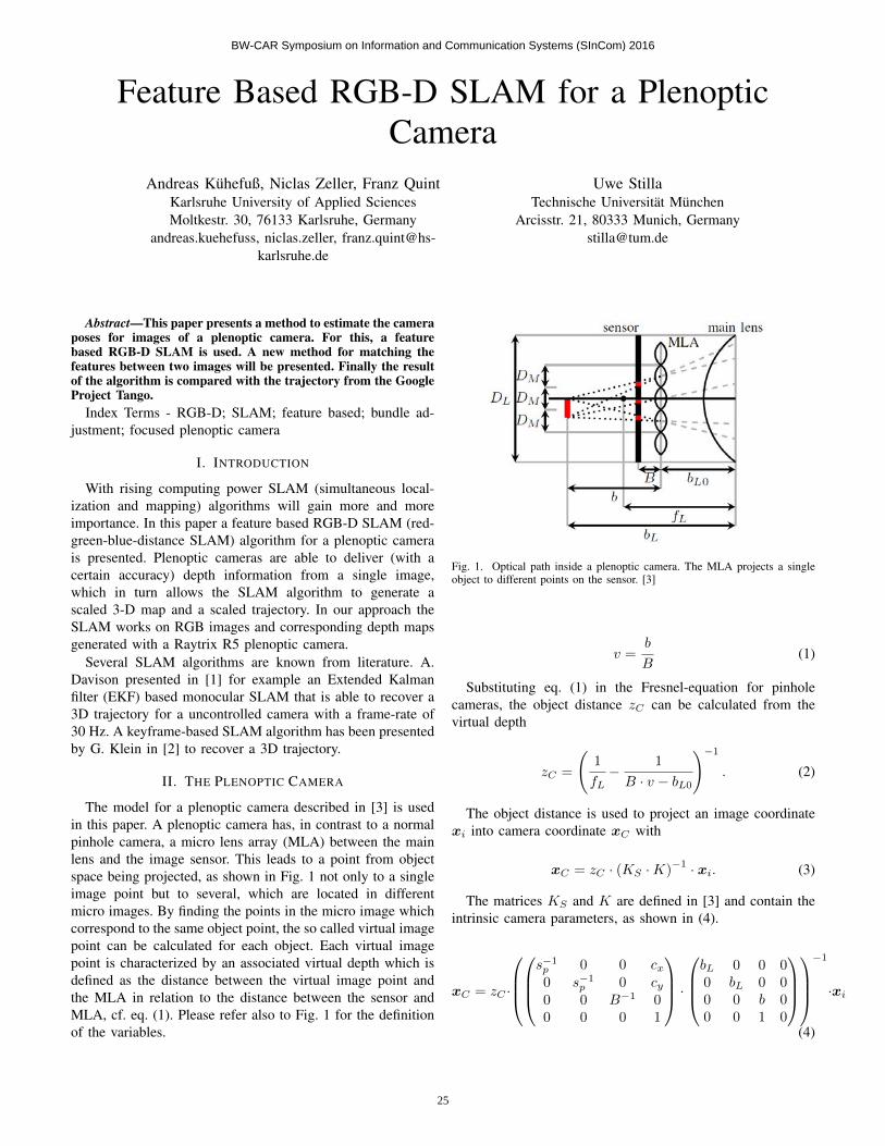
Feature Based RGB-D SLAM for a PlenopticCamera

Andreas Kuhefuß, Niclas Zeller, Franz QuintKarlsruhe University of Applied SciencesMoltkestr. 30, 76133 Karlsruhe, Germany

andreas.kuehefuss, niclas.zeller, [email protected]

Uwe StillaTechnische Universitat Munchen

Arcisstr. 21, 80333 Munich, [email protected]

Abstract—This paper presents a method to estimate the cameraposes for images of a plenoptic camera. For this, a featurebased RGB-D SLAM is used. A new method for matching thefeatures between two images will be presented. Finally the resultof the algorithm is compared with the trajectory from the GoogleProject Tango.

Index Terms - RGB-D; SLAM; feature based; bundle ad-justment; focused plenoptic camera

I. INTRODUCTION

With rising computing power SLAM (simultaneous local-ization and mapping) algorithms will gain more and moreimportance. In this paper a feature based RGB-D SLAM (red-green-blue-distance SLAM) algorithm for a plenoptic camerais presented. Plenoptic cameras are able to deliver (with acertain accuracy) depth information from a single image,which in turn allows the SLAM algorithm to generate ascaled 3-D map and a scaled trajectory. In our approach theSLAM works on RGB images and corresponding depth mapsgenerated with a Raytrix R5 plenoptic camera.

Several SLAM algorithms are known from literature. A.Davison presented in [1] for example an Extended Kalmanfilter (EKF) based monocular SLAM that is able to recover a3D trajectory for a uncontrolled camera with a frame-rate of30 Hz. A keyframe-based SLAM algorithm has been presentedby G. Klein in [2] to recover a 3D trajectory.

II. THE PLENOPTIC CAMERA

The model for a plenoptic camera described in [3] is usedin this paper. A plenoptic camera has, in contrast to a normalpinhole camera, a micro lens array (MLA) between the mainlens and the image sensor. This leads to a point from objectspace being projected, as shown in Fig. 1 not only to a singleimage point but to several, which are located in differentmicro images. By finding the points in the micro image whichcorrespond to the same object point, the so called virtual imagepoint can be calculated for each object. Each virtual imagepoint is characterized by an associated virtual depth which isdefined as the distance between the virtual image point andthe MLA in relation to the distance between the sensor andMLA, cf. eq. (1). Please refer also to Fig. 1 for the definitionof the variables.

Fig. 1. Optical path inside a plenoptic camera. The MLA projects a singleobject to different points on the sensor. [3]

v =b

B(1)

Substituting eq. (1) in the Fresnel-equation for pinholecameras, the object distance zC can be calculated from thevirtual depth

zC =

(1

fL−

1

B · v − bL0

)−1

. (2)

The object distance is used to project an image coordinatexi into camera coordinate xC with

xC = zC · (KS ·K)−1 · xi. (3)

The matrices KS and K are defined in [3] and contain theintrinsic camera parameters, as shown in (4).

xC = zC ·

s−1p 0 0 cx0 s−1

p 0 cy0 0 B−1 00 0 0 1

·bL 0 0 00 bL 0 00 0 b 00 0 1 0

−1

·xi

(4)


25

The parameter bL is the distance of the virtual image tothe optical center of the main lens and is calculated using theFresnel equation for the main lens

bL =

(1

fL−

1

aL

)−1

. (5)

III. FEATURE ACQUISITION

This section describes which feature types are used and howfeatures are matched between images. First the raw images ofa plenoptic camera have to be converted into RGB and depthmap images. For this, the method presented in [4] is used.After feature extraction, a matching between features in twoconsecutive images is established.

A. Image acquisition

The scene is recorded with a plenoptic camera. Afterrecording, all raw images are converted to RGB and depth-map images, which in our case have the size 1024 x 1024pixels. To do this, we use the method presented in [4]. Thedepth map contains for each pixel a virtual depth, which iscoded as a 16-bit grayscale value. Conversion to the virtualdepth v cf. eq. (1) is performed as suggested in [5] with

v =1

1−grayscale16−bit

65535

. (6)

This virtual depth is used together with the internal cameraparameters fL, B and bL0, which have been determined in aprevious calibration step, to calculate the object distance zCwith eq. (2). Finally, the camera coordinates of a point can becalculated with eq. (3) out of the image coordinates.

Due to the small baseline between the micro images pro-jected by the MLA, estimation of the virtual depth froma single image of a plenoptic camera is possible within alimited accuracy. Depth estimation can be improved using thelarger baseline between successive images of a video. For this,corresponding points have to be matched. This is done witha new method, which we call Slope Matching and which ispresented in the following.

B. Slope Matching

Interesting points in the images of the video sequence aredetected using the SURF feature detector [6]. After detectingall SURF features in two consecutive images, a match foreach feature from the first image is searched in the second.This is done by looking for nearest neighbour with the methodpresented in [7] and considering the feature quality attributesdelivered by the SURF detector. The resulting matches for twoconsecutive images are shown in Fig. 2.

Fig. 2. Resulting matches for two consecutive images, after next neighborsearch.

As one can see in Fig. 2 there are many wrong matcheswhich have to be removed. To remove the wrong matches, wejust stick the two images side by side and calculate the slopeof the line connecting the matched points (blue lines in Fig.2) with

mi =yi,2 − yi,1

(xi,2 + 1024)− xi,1. (7)

After calculating the slope for each match, the median ofall slopes is computed. Each match will be marked as wrongif it doesnt satisfy condition (8), where ε is a suitably chosenthreshold.

mmedian − ε ≤ mi ≤ mmedian + ε (8)

Since the rotation and the translation between two consecu-tive images of a video is small, the slope for each match shouldbe within the limits given by ε. Inequation (8) removes allmatches with slopes that differ significantly from the median.

After this operation there still might remain wrong matches,e.g. between a feature from the very left of the first image toa feature of the very right in the second image, but having theslope similar to the median. To remove these wrong matches,the two pictures are stacked one above the other and theprevious step is repeated. Mathematically this is done bycalculating the inverse slope m

′

i of the matches

m′

i =xi,2 − xi,1

(yi,2 + 1024)− yi,1. (9)

Again the median will be determined and a constraintsimilar to the one presented in ineq. (8) removes all matcheswith a wrong slope. The result of both slope filters is shownin Fig. 3.

Fig. 3. Resulting matches for two consecutive images, after next neighborsearch and slope filters.


26

The resulting matches will be used for pose estimationbetween two consecutive images.

Fig. 4. Feature chain between three images.

The baseline can be further extended, if matches are notrestricted to consecutive images. For this we use a featurechain as shown in Fig. 4. If a feature is matched between thefirst and the second and also between the second and the thirdimage, the feature from the first image is linked to the featurefrom the third image. The yellow x in the third image showsan feature that could not be matched. The feature chain isbroken for this feature.

IV. POSE ESTIMATION

Pose estimation is divided into two parts: First initialposes are estimated between two consecutive images. Afterestimating enough poses, a local bundle adjustment will beperformed.

A. Transformation Matrix

To estimate the pose for two consecutive images, thetransformation matrix has to be estimated. The transformationmatrix is defined by three rotations and three translations.These six parameters form the camera vector a as shown ineq. (10) and need to be estimated for every new image.

a =(α β γ tx ty tz

)T(10)

B. Initial pose estimation

Instead of estimating the twelve (mutually dependent) ele-ments of the transformation matrix in homogeneous coordi-nates between the camera coordinate systems of two images,we estimate directly the six elements of a with an iterativeprocedure.

The first pose is estimated using the results of the slopematching shown in Fig. 3. First the features are projected fromthe image coordinate system in the camera coordinate systemusing eq. (4). Now they can be transformed from the cameracoordinates corresponding to the first image in the cameracoordinates corresponding to the second image. This is doneby multiplying the coordinates with the transformation matrixT as shown in (11).

x′

C = T · xC (11)

The transformation matrix T is the one which is determinedby the vector a to be estimated. At the beginning of theiterative process, the matrix is initialized with the identitymatrix.

The coordinates of the features from the first image in thecamera coordinate system of the second image can be back-projected in the image coordinate system if the second imageby using the inverse of eq. (3), as shown in (12).

x′

i =1

zC· (KS ·K) · x

′

C (12)

Note that the matrix Ks is the same for both images sincethe camera remains unchanged. The matrix K however needsto be adapted, since it depends on bL, which is a functionof the virtual depth (see eq. (5)). After transforming everyfeature of the first image into the second image (initially withthe identity matrix), there will remain a reprojection error foreach match, expressed as the difference between the positionvector of a feature from the first image transformed to thesecond image and its match in the second image (eq. (13)).The position vectors are three-dimensional since they describepoints in the virtual image. The third dimension in the virtualimage is the virtual depth.

rj (a) = x′

ij − xij =

x

′

ij

y′

ij

v′

ij

1

−xijyijvij1

(13)

The goal is to find the camera vector a (and thus implicitlythe transformation matrix T ) which minimizes the meanreprojection error over all matches:

a′= min

a

n∑j=1

||rj (a)|| (14)

To solve the minimization problem, the Gauss-Newton algo-rithm is applied. To minimize the impact of outliers, Tukeysbiweight cost function is used [8]. This function suppressesoutliers by weighting them with zero, as shown in (15).

wTb =

(1−

r2jσ2

)2

|rj | ≤ σ

0 |rj | > σ

(15)

By weighting large outliers with zero, wrong matches willnot influence the estimation. For calculating the weight wTb,the empirical standard deviation σ of the errors is used.

C. Bundle adjustment

To optimize the camera position for more than just twoimages a local bundle adjustment [9] is performed. The bundleadjustment is called local since is not carried out over allimages (frames) of the sequence, but only from a so calledkey-frame to the next key-frame. A new key-frame is set,if the number of matches in a feature chain (see Figure 4)falls below a threshold. In our experiments we have set a newkey-frame when the number of matches has fallen below athreshold. However, even if the number of matches exceeds thethreshold, every sixth frame is set as a key-frame to ensure that


27

the bundle adjustment is executed with a sufficient frequencyto prevent a drift.

The m images contained between the two key-frames partic-ipate in the local bundle adjustment with their camera vectorsak. Consider that for a total of n world points bj matches havebeen found. The world points are given by their homogeneouscoordinate vector

bj =(xwj

ywjzwj

1)T. (16)

The residual error of the world points, projected in thecorresponding frames depends of course on the camera vectorsak as shown in eq. (17)

rjk (ak, bj) = x′

ijk(ak, bj)− xijk . (17)

The image coordinates used to calculate the error areobtained by projecting the world points in the correspondingframes using eq. (18), which is similar to eq. (12)

x′

ijk(ak, bj) = Tak

·1

zwk

· (KS ·K) · bj . (18)

The task of the bundle adjustment is to find the parameterswhich minimize the mean error over the n world points andm camera positions with

{a

′

k, b′

j

}= min

ak,bj

m∑k=1

n∑j=1

||rjk (ak, bj)|| . (19)

To minimize the effect of outliers, we use in this step alsoTukeys biweighted function (15).

V. EVALUATION

To evaluate the presented RGB-D SLAM algorithm, twoexperiment setups have been made. The first is a set of 40images with known ground truth and the second is a set of1974 images where the trajectory is compared with the oneestimated by the Project Tango of Google. Example imagesfor both experiments are shown in Fig. 5 and Fig. 6.

Fig. 5. Image 20 / 40 of the firstexperiment

Fig. 6. Image 800 / 1974 of thesecond experiment

A. Comparison with ground truth

The first experiment contains a small number of 40 imageswhich have been recorded in a known grid. First, the camerawas moved 19 cm to the right in one cm steps. After thatthe camera was moved 10 cm back, again in steps of 1 cmeach. At last, the camera was moved 19 cm back to the left,in 2 cm steps. The last step amounted again to one cm. Thusthe camera was at the end of the movement 10 cm behindits start position. The result of the RGB-D SLAM without abundle adjustment is shown in Fig. 7. The blue cones markthe position and the orientation of the camera as estimated byour SLAM algorithm without bundle adjustment. The whitecones show the ground truth.

Fig. 7. Result for the first experiment, without bundle adjusment. Blue conesmark the estimated trajectory, the white ones the ground truth.

As one can see in Fig. 7 there is a big drift when not usinglocal bundle adjustment. The trajectory for the same imageswith local bundle adjustment is shown in Fig. 8.

Fig. 8. Result for the first experiment, with bundle adjusment. Blue conesmark the estimated trajectory, the white ones the ground truth.

As one can see in Fig. 8 the estimated trajectory fits wellto the known ground truth. The drift error is compensated bythe local bundle adjustment.

B. Comparison with Google Project Tango

The second experiment was done on a longer trajectory,using 1974 images. To evaluate the result, the experiment wasrecorded in parallel with the plenoptic camera and with a tablet


28

fixed to the plenoptic camera. On the tablet Google ProjectTango was running. The software of Project Tango estimatesa 3D trajectory using a accelerometer and a monocular camera[10]. The trajectories resulting from our RGB-D SLAM andfrom Project Tango are compared qualitatively. Of course theresult of Google Project Tango is not the actual ground truth,but also subject to errors. However, it is a quite good estimate.

Fig. 9. Result for the second experiment. Red trajectory is from RGB-DSLAM and the black one is from Google Project Tango. Scale is in mm.

Fig. 10. Result for the second experiment. Red trajectory is from RGB-DSLAM with corrected scale and the black one is from Google Project Tango.Scale is in mm.

The result of the second experiment is shown in Fig. 9. Theestimated trajectory matches qualitatively with the trajectoryfrom Google Project Tango, but as one can see there is ascaling error in the data. For better comparison we estimatedthe scale error using CloudCompare [11]. After correcting ourtrajectory with the estimated scale, which amounted to 1.125,the comparison can be performed easier. It is shown in Fig.10.

As one can see in Fig. 10, the two trajectories fit quitewell. There is still a very small offset, observable in the topleft of the figure. To minimize also this offset a global bundleadjustment could be performed.

VI. CONCLUSION

The presented method works quite well for typical videosrecorded with the plenoptic camera. The matching methodsupplies good and enough matches for the trajectory estimationto work stable, even for a long scene as shown in the secondexperiment. Nevertheless there remain some unsolved prob-lems like the scaling error shown in Figure 9. This error hasbeen corrected up to now only interactively and an automatedprocedure has to be implemented. Furthermore would a global

bundle adjustment using the key-frames only help to achievehigher stability against drift.

VII. ACKNOWLEDGMENT

This research was done in the Bachelor Thesis of AndreasKuhefuß. It is part of the project Mosyko3D, which is fundedby the Baden-Wrttemberg-Stiftung in its program Photonics,Microelectronics, Information Technology. We gratefully ac-knowledge the support.

REFERENCES

[1] A. Davison, I. Reid, N. Molton and O. Stasse, ”MonoSLAM: Real-Time Single Camera SLAM” IEEE Transactions on Pattern Analysis andMachine Intelligence Vol. 29, nr. 6, p. 1-16, 2007.

[2] G. Klein and D. Murray, ”Parallel Tracking and Mapping for Small ARWorkspaces”, Proc. International Symposium on Mixed and AugmentedReality, ISMAR’07, Nara, 2007.

[3] N. Zeller, F. Quint and M. Stterlin, ”Investigating Mathematical Modelsfor Focused Plenoptic Cameras”, Proc. of International Symposium onElectronics and Telecommunications ISETC2016, p. 285-288, Timisoara,2016.

[4] N. Zeller, F. Quint, U. Stilla, ”Establishing a Probabilisitc Depth Mapfrom Focused Plenoptic Cameras”, Proc. International Conference on 3DVision (3DV), p. 91-99, Lyon, 2015.

[5] ”Converting Depth Data,” www.raytrix.de, Raytrix GmbH, 2013.[6] H. Bay, T. Tuytelaars, L. Van Gool, ”SURF: Speeded Up Robust Fea-

tures”, Journal on Computer vision and image understanding, vol. 110,nr. 3, p.346-359.

[7] M. Muja, D. Lowe, ”Fast Approximate Nearest Neighbors With Auto-matic Algorithm Configuration”, International Conference on ComputerVision Theory and Application VISSAPP’09, INSTICC Press, p. 331-340, 2009.

[8] R. Maronna, D. Martin, V. Yohai: Robust statistics: Theory and methods,Wiley Series in Probability and Statistics, Chichester: John Wiley & Sons,2006.

[9] R. Hartley, A. Zisserman: Multiple View Geometry in Computer Vision.Cambridge University press, 2004.

[10] ”Google Project Tango”, www.google.com/tango/, 2016.[11] ”CloudCompare”, www.cloudcompare.org, 2016.


29


30

A Comparative Study ofData Clustering Algorithms

Ankita Agrawal and Artur SchmidtInstitue for Artificial Intelligence

University of Applied Sciences, Ravensburg-Weingarten, GermanyEmail: [email protected]

Abstract—Cluster analysis is important for understanding thestructure of a particular data set. This paper compares someknown clustering algorithms. The criteria for comparison areusability (choice of initial input parameters), simplicity, accuracyand computational complexity. The aim is to search for anoptimal clustering algorithm by evaluating its performance ondata sets from different fields of application. Other related topics,scaling and cluster validation are also discussed.

I. INTRODUCTION

The goal of this paper is to understand various clusteringalgorithms and to provide an unbiased evaluation based oncomparison criteria. Clustering is the grouping of data intoclusters such that the data vectors in one cluster are moresimilar to each other than those in another cluster. A dataset X = (x1, . . . , xn) consists of n d-dimensional vectors,xi ∈ X ⊆ Rd.Clustering is the unsupervised learning problem of findinga structure in a set of unlabeled data, where the correctclusters are not previously defined. It is used for data miningtechniques in many fields, such as, medicine [1], psychology[2], marketing [3], biology [4], linguistics [5]. Clustering isused to find internal structures in the data, such as, reoccurringpatterns and anomalies. Also, it is usually the pre-processingstep for many other algorithms, such as artificial intelligencetechniques. For comparison, we chose popular clustering algo-rithms based on different working principles as given below.a) Centroid-based (K-means, Kernel k-means, Spectral)b) Distribution-based (EM Algorithm)c) Connectivity-based (Hierarchical)d) Density-based (DBSCAN, OPTICS)

II. METRICS

A. Distance

The performance of a clustering algorithm depends criticallyon a good distance metric in the input space that reflectsthe relationship between a given data. A metric is a functiondefining the distance between each pair of elements or vectorsin a data set. For example, the Minkowski distance given by,d : X × X → R+

0 , where R+0 = {t ∈ R | t ≥ 0}.

d(x, y) =

(d∑

i=1

|xi − yi|p)1/p

is a generalized form. The widely used distances are

Manhattan-distance (p = 1), Euclidean-distance (p = 2)and Chebyshev-distance (p = ∞). We used primarily theEuclidean distance as it is translation and rotation invariant.

B. Scaling

Scaling or data normalization is a pre-processing step forclustering. The range of data values for different dimensionsmay vary greatly, thereby causing one or more dimensions tostrongly influence the result. Scaling ensures the proportionalcontribution of each dimension.We used Min-Max Scaling (rescaling the values of all dimen-sions to a target range), defined as,

xli,norm =

xli − minj∈[1,n]

(xlj)

maxj∈[1,n]

(xlj)− minj∈[1,n]

(xlj), where l ∈ [1, d] ⊆ N

and Standardization (values of each dimension have zero-meanand unit-variance), defined as,

xi,norm =xi −mean(x)

var(x)

For comparison, we also used Multi-Dimensional Scaling(MDS) [6] to detect relevant dimensions that represent thesimilarities within data.

III. CLUSTER VALIDATION

Every clustering algorithm can find a set of clusters, whetherthe structure exists in the data or not. Even the order of data orchoice of different input parameters for the same algorithm canlead to very different clustering results. Therefore, validationof the cluster quality becomes very important. The silhouettecriterion for evaluating the clustering quality is defined asfollows.

A. Silhouette Criterion

The Silhouette criterion [7] takes as input the final set ofclusters C obtained from a clustering algorithm. It measureshow closely the data matches to other data within its owncluster and how loosely it matches to data in other clusters. Itreturns the value S on the interval [−1,+1] where +1 indicatesthat the data is appropriately clustered and vice-versa.

s(xi) =b(xi)− a(xi)

max{a(xi), b(xi)}and S =

1

n

n∑i=1

s(xi)


31

Here, a(xi) is the average distance of xi to other data withinthe same cluster and b(xi) is the lowest average distance ofxi to any other cluster.

IV. CLUSTERING ALGORITHMS

The algorithms take as input the data set X ∈ Xn. Theoutput is 1 ≤ k ≤ n clusters C = {C1, . . . , Ck}, where Ci isa mutually exclusive subset of X.

A. K-Means

We implement the k-means algorithm as proposed in [8],which partitions the data into k clusters by iteratively minimiz-ing the within-cluster sum of squares with k chosen manuallya priori. The algorithm alternates between two steps, firstlyassigning each data vector to the cluster with the nearestcluster mean and secondly, re-calculating the new mean forthe updated clusters. The objective is to find the clusters suchthat, argmin

C

∑ki=1

∑x∈Ci

‖x− µi‖2, where µi ∈ X is the

mean of vectors in Ci.We analyzed the following two methods to select the initialcluster centers. First, randomly choose k vectors from thedata set X as initial means. Second, k-means++ [9] algorithmis used, where a subsequent cluster center in an iteration ischosen with probability proportional to its squared distancefrom the existing cluster centers.

B. Kernel K-Means

Kernel k-means applies k-means algorithm in kernelspace as proposed in [10]. The data points are mappedfrom input space to a higher dimensional space withφ : X → H and then k-means is performed in thistransformed space. The k-means equation changes toargmin

C

∑ki=1

∑x∈Ci

‖φ(x)− µi‖2, where µi ∈ H is mean

of vectors in Ci in the transformed space.

C. Spectral Clustering

Spectral clustering [11] uses eigenvectors of similarity ma-trix (also known as kernel or Gram matrix) calculated fromthe input data. A dimensionality reduction is performed bytaking the k largest eigenvectors as columns to obtain a n×kmatrix. Clustering is performed on this reduced matrix withnew input vectors Y = (y1, . . . , yn), where yi is the reducedtransformed vector of xi in the higher dimensional space H.

D. Expectation-Maximization Algorithm

EM algorithm [12], assumes that the data set can bemodeled as a combination of multivariate normal distributions.It finds the maximum-likelihood estimate of the parameters ofan underlying distribution in a statistical model for a data setX. Here, besides initial cluster centroids, initial co-variancematrices and probability distribution of each cluster are alsorequired as input parameters.

E. Hierarchical Clustering

We use the single-linkage variant of the agglomerativehierarchical clustering suggested independently by McQuitty[13] and Sneath [14]. Initially each input vector is in its owncluster. At each step, the two clusters separated by the leastdistance are merged. The distance d between two clusters isdefined as d(Ci, Cj) = min

p∈Ci,q∈Cj

d(p, q).

The process goes on until the termination criterion is reached(in our case, number of desired clusters).

F. DBSCAN

DBSCAN (Density-Based Spatial Clustering of Applica-tions with Noise) [15] is an algorithm which forms clustersbased on the local density of data points. It requires twoinput parameters, MinPts (the number of points required toform a cluster) and ε (neighborhood size). The data points areassigned to a cluster if the minimum number of neighbouringpoints specified at the beginning are present, otherwise it isclassified as noise.

G. OPTICS

OPTICS (Ordering Points To Identify the Clustering Struc-ture) [16] builds upon DBSCAN so that only one parameteris needed for clustering. It addresses the major drawback ofDBSCAN clustering, which is, not being able to find clusterswith different densities. The input parameters are MinPts andγ (maximum distance to consider for a cluster). The value ofγ influences the time complexity of the algorithm and thecluster quality. However, in OPTICS, the output is difficultto interpret, especially with large data count. The output is aparticular ordered list of data from the input data set accordingto their smallest reachability distance, which is the distance ofa data point xi to it’s MinPts-th closest point.

V. EXPERIMENTS

A. Datasets

For evaluating performance of the clustering algorithms, weused pre-labeled data sets available in [17] and 2-dimensionalsynthetic data from [18]. The data sets, summarized in TableI, were chosen from various fields of application, so as to finda general plausible algorithm.

B. Comparison of Algorithms

This section details how the experiments were carried out.Four variants of data are used, unscaled and scaled data usingthe three techniques mentioned in Section II-B. The clusteringalgorithms are then executed with the initial values requiredby the individual algorithms. Below are the additional detailsabout the algorithms in our implementation.The initial centroids in k-means algorithm are selected fromthe data using k-means++ algorithm, as it distributes thecentroids in the data space, increasing the probability for betterresults. For kernel k-means and spectral clustering, Gaussianand polynomial kernels are used to form the similarity matrix.In EM algorithm, k-means with k-means++ initialization isapplied to find the initial clusters and then EM algorithm


32

TABLE I: Details of the Data Sets

Data Dimen- NumData set Count sions Class Description

Medicine, diagnosis ofAppendicitis 473 15 2 appendicitis [20]Iris 150 4 3 Botany, iris plant typesMovement Video, hand movement inLibra 360 90 15 Brazilian sign language

Agriculture, three differentSeeds 210 7 3 varieties of wheat

Medicine, analysis ofThyroid 215 5 3 thyroid diseaseUser Knowle- Knowledge, studentdge Modeling 403 5 4 knowledge level [21]Wholesale Business, clients of aCustomers 440 7 2 wholesale distributor [22]Wine 178 13 3 Food, wine origin/type

Food, cellular localiza-Yeast 1484 8 10 tion sites of proteinsAggregation 788 2 7 Synthetic dataCompound 399 2 6 Synthetic dataPathbased 300 2 3 Synthetic dataR15 600 2 15 Synthetic data

is carried out to optimize the log likelihood function. Toovercome the problem of an infinite log value resulting from asingular covariance matrix caused by numerical computationof matrix determinant, a random value between 0 and 0.01 isadded repeatedly to the diagonal elements in the covariancematrix till a positive determinant value is obtained.In OPTICS, the value of γ is set to maxxi,xj

d(xi, xj),eliminating the need for a second input parameter and theclusters adjust themselves according to the density of datapoints in a particular region. In the output list, the datahaving low reachability are aligned together, showing that theybelong to the same cluster. When the reachability distanceshows a jump, it indicates the start of another cluster. Ourimplementation looks for this sudden jump by comparing therelative difference in distances of current datum in the list toits previous two data, thus selecting the resulting clusters.Each algorithm is executed five times for each data set andthe average of all results (clustering accuracy) along with thevariance is taken as the final result for an algorithm on adataset. The optimal values for some initial parameters arefound using cross-validation, such as σ in Gaussian kernel forkernel k-means and spectral clustering. The details about theclustering algorithms are listed in Table II.

VI. RESULTS

In this section, the results obtained for the algorithms arediscussed. Figure 1 shows the clustering results on the Ag-gregation data set. We can see that k-means linearly separatesthe data whereas spectral is able to cluster the data perfectly.Hierarchical clustering and OPTICS give similar result. Thetwo connected clusters on the right side and bottom left cornerare combined as one cluster. As mentioned in Table II, it canbe seen that a large k does not affect the result of hierarchicalclustering. Since, the cluster number is given as 7 initially,

only one (in blue) and two (in gray) data points are assignedto the remaining two clusters, not much affecting the errorrate.

(a) K-Means (k = 7) (b) Kernel K-Means (k = 7, σ = 0.2)

(c) Spectral (k = 7, σ = 0.7) (d) EM (k = 7)

(e) Hierarchical (k = 7) (f) OPTICS (MinPts = 10)

Fig. 1: Clustering results on the Aggregation data set. Eachcluster is depicted by a different color. The input parametervalues for each algorithm are also mentioned. For Kernel k-means and Spectral algorithms, a Gaussian kernel is used.

Figure 2 and 3 represent the output of OPTICS algorithm andits interpretation as clusters. In Figure 2a, it can be easilyseen that there are 15 clusters. Here, it is also not difficult toconvert the list to clusters, as can be seen in Figure 2b. TheR15 data set is correctly clustered by all the algorithms. Onthe other hand, Figure 3a shows that the first cluster can endeither around 50 or 140 data points. It is not a trivial taskto write a generalized algorithm that could convert the listto clusters appropriately. Even if the list is ordered correctly,the conversion may not be accurate. The results of DBSCANare worse than OPTICS and hence, are not discussed here.The clustering results for the Compound data set are shown inFigure 4. Here, spectral clustering does not cluster the data inthe lower left corner correctly because the clusters consist of


33

TABLE II: Properties of Clustering Algorithms and their Complexity (n=data count, k=number of clusters, d=dimensions,i=number of iterations)

Algorithm Input Parameters Constraints Positives ComplexityK-means # of clusters, initial k centroids linear separation, local min-

ima, no outlier detection, verysensitive to initial centroids

easy to understand and implement,fast if k is small, even with largedata

O(nkdi)

Kernel k-means # of clusters, k centroids, standarddeviation σ (gaussian), degree dand constant c (polynomial kernel)

slow due to computation ofkernel matrix, esp. for largedata, requires tuning of kernelparameters

k-means applied in kernel space,minimizes clustering error in thetransformed space

O(n2 + nkdi)

Spectral # of clusters, k centroids, standarddeviation σ (gaussian), degree dand constant c (polynomial kernel)

computationally expensive dueto computation of kernel ma-trix and eigen values

kernel PCA to reduce dimension-ality, effective for both low- andhigh-dimensional data

O(n3)

EM # of clusters, k means, k variance,k probability distribution

numerical problems fast given good initialization, effec-tive for high-dimensional data

O(n2 + nkdi)

Hierarchical # of clusters sensitive to order of points fast, simple, large k does not affectthe result

O(n2)

DBSCAN neighbors MinPts, distance ε can not identify varied densityclusters

insensitive to order of points andnoise

O(n2)

OPTICS neighbors MinPts, max. distanceγ

output as ordered list and notclusters

filter noise, can detect varied den-sity clusters.

O(n2)

0 100 200 300 400 500 600

ordered data points

reac

habi

lity-

dist

ance

(a) Ordered Output List

x

y

(b) Interpreted Clusters

Fig. 2: The clustering output of OPTICS for the R15data set with MinPts = 10 is shown in (a). Thereachability distance for each data point is plotted on they − axis. The interpretation of the list into clusters is shownin (b).

0 50 100 150 200 250 300

ordered data points

reac

habi

lity-

dist

ance

(a) Ordered Output List

x

y

(b) Interpreted Clusters

Fig. 3: The clustering output of OPTICS for the Path-based data set with MinPts = 3 is shown in (a). Thereachability distance for each data point is plotted on they − axis. The interpretation of the list into clusters is shownin (b).

(a) K-Means (k = 6) (b) Kernel K-Means (k = 6, σ = 0.7)

(c) Spectral (k = 6, σ = 0.7) (d) EM (k = 6)

(e) Hierarchical (k = 6) (f) OPTICS (MinPts = 4)

Fig. 4: Clustering results on the Compound data set.


34

different structures. Hierarchical clustering forms appropriateclusters based on the distance function but not according tothe correct labels. OPTICS algorithm identifies the clustersaccurately except the ones in the upper left corner. The otheralgorithms do not give satisfying results.The results for the multi-dimensional data sets are presentedin Table III. It contains sub-parts for the clustering performedon data with different scaling methods. Each element of thetable represents average percentage of data points that arecorrectly clustered over multiple executions of the algorithmson each data set and variance in the results. The results forhierarchical clustering and OPTICS algorithm remain samefor each iteration, and hence, the variance is not mentioned.For other algorithms, the results in each iteration vary withdifferent initial parameters, so the variance is relevant. Thecombination of higher percentages and lower variances foreach data set is highlighted in the table. The average forunscaled data is 65.1±2.4%, for MinMax scaling 67.4±1.9%,57.0 ± 2.5% for Standardization and 63.8 ± 2.1% for Multi-Dimensional scaling. It can be seen that for almost all datasets, there is 6 − 7% drop in the clustering accuracy withStandardization. On the other hand, with MinMax scaling,the clustering result either improves or stays the same. Wecan also see that the k-means, kernel k-means, hierarchicalclustering and OPTICS algorithm either have no best resultsor only for one or two data sets. K-means works only good forlinearly separable data. Kernel k-means performs only slightlybetter than k-means. Hierarchical clustering yields good resultsfor 2-dimensional data but does not handle high-dimensionaldata well. It is found that silhouette criterion does not providethe optimal cluster count. This is because it uses Euclideandistance, which prefers linearly-separable spherical structures.We executed silhouette on the top of EM algorithm for thedata sets and the results got worse. E.g. for the Iris data set,silhouette returned the optimal cluster count as 2 instead of3 and the accuracy reduced from 98% to 66.7%. Due to thelack of an efficient algorithm to convert the output orderedlist to clusters, OPTICS often produces high error rate infinal clustering result. In general, spectral clustering gives bestresults as it applies PCA to data in the transformed high-dimensional space to extract those dimensions having the mostimportant information about the data set. EM algorithm, whichdoes not give good results for two-dimensional data and doesnot converge for Movement Libra data set, gives the bestresults for high-dimensional data. It optimizes the Gaussiandistribution for each dimension to find clusters with differentshapes in a data set, thereby improving the result.

VII. CONCLUSION

The results show that overall Spectral clustering and EMalgorithm give the best results for most real data sets. However,Spectral clustering is computationally expensive due to kernelmatrix and eigenvalue calculation and is very slow for largedata sets. Therefore, it is recommended to use EM algorithmwhere the initial clusters are given by k-means with k-means++ algorithm.

MinMax Scaling is fast and also has the highest averagepercentage for all datasets, making it the favorite choice amongthe scaling methods.

REFERENCES

[1] R. Xu and D. C. Wunsch, Clustering Algorithms in Biomedical Research:A Review, Biomedical Engineering, IEEE Reviews, 3, 120-154, 2010.

[2] J. Clatworthy, D. Buick, M. Hankins, J. Weinman and R. Horne, The useand reporting of cluster analysis in health psychology: A review, BritishJournal of Health Psychology, 10, 329-358, 2005.

[3] H. Lai and T.-C. Yang, A group-based inference approach to customizedmarketing on the Web integrating clustering and association rules tech-niques, System Sciences, Hawaii International Conference, 10, 2000.

[4] A. C. Tan and D. Gilbert, An Empirical Comparison of SupervisedMachine Learning Techniques in Bioinformatics, APBC 2003.

[5] V. Hatzivassiloglou, L. Gravano and A. Maganti An investigation of lin-guistic features and clustering algorithms for topical document clustering,SIGIR, 224-231, 2000.

[6] J. B. Kruskal and M. Wish, Multidimensional Scaling, Sage UniversityPaper series on Quantitative Application in the Social Sciences, 7-11,1978.

[7] P. J. Rousseuw, Silhouettes: a Graphical Aid to the Interpretation andValidation of Cluster Analysis, Computational and Applied Mathematics,20, 53-65, 1987.

[8] S. P. Lloyd, Least Squares Quantization in PCM, IEEE Transactions onInformation Theory, 28(2), 129-137, 1982.

[9] D. Arthur and S. Vassilvitskii, k-means++: the advantages of carefulseeding, ACM-SIAM symposium on Discrete algorithms, Society forIndustrial and Applied Mathematics Philadelphia, USA, 1027-1035, 2007.

[10] B. Schlkopf, A. Smola and K.-R. Mller, Nonlinear Component Analysisas a Kernel Eigenvalue Problem, Neural Computation, 10, 1299-1319,1998.

[11] A. Y. Ng, M. I. Jordan and Y. Weiss, On spectral clustering: Analysisand an algorithm, Advances in Neural Information Processing Systems,Cambridge, MA, 14, 849-856, 2002.

[12] A. P. Dempster, N. M.Laird and D. B. Rubin, Maximum Likelihood fromIncomplete Data via the EM Algorithm, Journal of the Royal StatisticalSociety, Series B (Methodological), 39(1), 1-38, 1977.

[13] L. L. McQuitty, Elementary Linkage Analysis for Isolating Orthogonaland Oblique Types and Typal Relevancies, Educational and PsychologicalMeasurement, 17, 207-229, 1957.

[14] P. H. A. Sneath, The Application of Computers to Taxonomy, Journal ofGeneral Microbiology, 17, 201-226, 1957.

[15] M. Ester, H. Kriegel, J. Sander and X. Xu, A density-based algorithm fordiscovering clusters in large spatial databases with noise, KDD, 226-231,1996.

[16] M. Ankerst, M. M. Breunig, H. Kriegel and J. Sander, OPTICS:Ordering Points To Identify the Clustering Structure, ACM SIGMODinternational conference on Management of data, 49-60, 1999.

[17] M. Lichman, UCI Machine Learning Repository http://archive.ics.uci.edu/ml, Irvine, CA: University of California, 2013.

[18] School of Computing, University of Eastern Finland, Clusteringdatasets, Retrieved from http://cs.joensuu.fi/sipu/datasets/.

[19] W. Ertel and M. Schramm, Combining Expert Knowledge and Data viaProbabilistic Rules with an Application to Medical Diagnosis, In UAI-2000 Workshop on Fusion of Domain Knowledge with Data for DecisionSupport, Stanford CA, 2000.

[20] W. Ertel and M. Schramm, Combining Data and Knowledge by MaxEnt-Optimization of Probability Distributions, In PKDD’99, Prague, 1704 ofLNCS, 323-328, 1999.

[21] H. T. Kahraman, S. Sagiroglu and I. Colak, Developing intuitive knowl-edge classifier and modeling of users’ domain dependent data in web,Knowledge Based Systems, 37, 283-295, 2013.

[22] N. Abreu, Analise do perfil do cliente Recheio e desenvolvimento de umsistema promocional, ISCTE-IUL, Lisbon, 2011.

[23] W. Jiang and F. L. Chung, Transfer Spectral Clustering, ECML PKDD,789-803, 2012.

[24] B. Boden, M. Ester and T. Seidl, Density-Based Subspace Clustering inHeterogeneous Networks, ECML PKDD (1), 149-164, 2014.

[25] G. Tzortzis and A. Likas, Ratio-based Multiple Kernel Clustering,ECML PKDD (3), 241-257, 2014.

[26] Y. Ren, U. Kamath, C. Domeniconi and G. Zhang, Boosted Mean ShiftClustering, ECML PKDD (2), 646-661, 2014.


35

TABLE III: Clustering Results - Correctly classified data along with variance over multiple runs of an algorithm for a data set(in %). The last column gives the mean percentage accuracy for an algorithm (average of the columns in a row).

Appendicitis Iris Libra Seeds Thyroid User K.M. Wholesale Wine YeastScaling - None

64.6 88.7 47.6 89.1 80.7 56.4 74.9 68.8 50.6 69.0K-means ± 0.6 ± 0 ± 2.4 ± 0 ± 5.4 ± 8.3 ± 2.2 ± 1.4 ± 2.7 ± 2.5K. k-means 64.4 87.8 46.1 89.3 81.3 59.1 73.5 69.7 52.2 69.3(gaussian) ± 0.8 ± 1.5 ± 3.1 ± 0.2 ± 4.8 ± 5.7 ± 6.9 ± 0.5 ± 2 ± 2.8K. k-means 64.5 86.3 46.8 89.3 81.1 56.9 71.9 69.7 50.8 68.6(polynomial) ± 0.7 ± 3 ± 2.1 ± 0.2 ± 5 ± 7.9 ± 8.5 ± 0.5 ± 2.6 ± 3.4Spectral 57 89.6 48.3 88.9 75.4 59.1 67.7 66.3 51.1 67.0(gaussian) ± 0 ± 2.4 ± 4.5 ± 1.6 ± 4.6 ± 3.2 ± 0 ± 1.7 ± 2.5 ± 2.3Spectral 57 96.7 49.3 82.5 85.9 56 75.1 41.3 51.1 66.1(polynomial) ± 0 ± 1.3 ± 1.8 ± 0.4 ± 1.1 ± 4.5 ± 0.6 ± 0.9 ± 1.6 ± 1.3

59 98 89.3 94.4 61 78.8 77.3 44.3 77.9EM ± 0.6 ± 0 - ± 2.1 ± 0.5 ± 5.6 ± 2.3 ± 7.6 ± 0.5 ± 2.1Hierarchical 57.5 68.0 12.5 37.1 70.7 32.8 67.7 43.3 32.4 46.9OPTICS 38.9 68.7 36.9 62.4 83.7 50.4 67.7 54.5 34.8 55.3

Scaling - MinMax71.2 88.4 46.4 88.8 88.8 57.4 67.7 94.9 53 72.9

K-means ± 0 ± 0.3 ± 1.9 ± 0.2 ± 0 ± 4.7 ± 0 ± 0 ± 2 ± 1.0K. k-means 71.2 84.8 46.2 88.8 88.2 55.7 67.7 94.8 53.1 72.3(gaussian) ± 0 ± 3.8 ± 4.6 ± 0.2 ± 0.7 ± 7.6 ± 0 ± 0.7 ± 2.5 ± 2.1K. k-means 71.2 78.9 47 88.8 87.8 53.6 67.7 94.6 52.3 71.3(polynomial) ± 0 ± 9.8 ± 3.3 ± 0.2 ± 1 ± 8.2 ± 0 ± 0.4 ± 2 ± 2.8Spectral 69.5 87.3 49.2 91.6 94.2 57.4 71.2 96.6 53.2 74.5(gaussian) ± 2 ± 2.7 ± 4.4 ± 2.7 ± 1.6 ± 3.6 ± 4.2 ± 1.2 ± 0.8 ± 2.6Spectral 71.3 81.2 49.7 89.4 90.3 53 67.7 93.4 51.4 72.0(polynomial) ± 0.9 ± 3.4 ± 3.1 ± 2.6 ± 1.3 ± 6.3 ± 0 ± 2.7 ± 1.9 ± 2.5

66.3 98 88.1 95.8 63.1 68.5 96.4 51.8 77.9EM ± 0.2 ± 0 - ± 0 ± 0 ± 3.2 ± 0.3 ± 0.3 ± 0.2 ± 1.0Hierarchical 57.5 66.7 12.22 34.8 72.1 32.8 67.7 39.9 32.4 46.2OPTICS 36.4 66.7 39.4 64.3 75.8 45.9 67.1 39.9 35.7 52.3

Scaling - Standardization57.9 75.3 45.9 51.2 78.8 40.5 67.7 61 51.1 58.8

K-means ± 0.6 ± 0 ± 2.7 ± 0.7 ± 2.1 ± 3.9 ± 0 ± 0.8 ± 0.8 ± 1.3K. k-means 57.5 73 46.8 51.7 77.4 45.5 67.7 58.3 50.3 58.7(gaussian) ± 1.1 ± 7.7 ± 3.4 ± 0.7 ± 3.5 ± 5.6 ± 0 ± 7 ± 2.5 ± 3.5K. k-means 57.5 57.8 46.4 51.6 77.4 39.2 67.7 57.9 49.7 56.1(polynomial) ± 1 ± 4.2 ± 5.8 ± 0.7 ± 3.5 ± 7.4 ± 0 ± 5.1 ± 2.3 ± 3.3Spectral 57.3 79.3 47.3 52 73.9 47.1 67.7 57.5 51.7 59.0(gaussian) ± 1.2 ± 2.1 ± 4.9 ± 1.8 ± 4.7 ± 5 ± 0 ± 7.1 ± 2.6 ± 3.3Spectral 59.4 81.4 42.2 55.5 78.7 36.6 67.7 58.4 53.4 59.2(polynomial) ± 3 ± 1.9 ± 2.8 ± 0.2 ± 1.4 ± 2.9 ± 0 ± 5.1 ± 0.4 ± 2.0

58.7 98 86.4 89.8 41.2 67.7 59.8 70.5EM ± 0.3 ± 1.3 - ± 1.2 ± 6.1 ± 1.1 ± 0 ± 3.7 - ± 1.5Hierarchical 58.5 68.0 12.2 36.2 72.6 32.5 67.7 39.9 32.2 46.6OPTICS 24.1 60.7 33.1 43.8 75.8 38.7 61.1 57.3 35.2 47.7

Scaling - MDS65.2 91.3 43.6 87.1 85.1 57.5 67.7 68.3 49.4 68.3

K-means ± 0 ± 0 ± 1.2 ± 0 ± 0 ± 7 ± 0 ± 0.8 ± 0.8 ± 1.1K. k-means 64.7 91.3 45.8 85.7 83.4 58 75.4 69.2 50.9 69.4(gaussian) ± 0.5 ± 0 ± 4.2 ± 1.4 ± 1.8 ± 6.5 ± 5 ± 1 ± 2.5 ± 2.5K. k-means 64.6 91.3 45.4 86.3 83.6 56.4 74.7 70 51 69.2(polynomial) ± 0.6 ± 0 ± 3.8 ± 0.9 ± 1.6 ± 8.1 ± 5.8 ± 0.2 ± 1.4 ± 2.5Spectral 57 91 43.6 85.8 72.3 60.4 67.4 51.9 66.2(gaussian) ± 0 ± 0.3 ± 7 ± 2.3 ± 5.9 ± 2.2 - ± 0 ± 1.6 ± 2.1Spectral 57 92 48.6 84.3 69.8 51.7 67.7 41.4 50 62.2(polynomial) ± 0 ± 2.7 ± 3.4 ± 3.3 ± 0 ± 8.4 ± 0 ± 1.3 ± 4.6 ± 3.0

63.8 90 85.2 95.4 61.6 67.7 71.2 49.5 72.8EM ± 0.2 ± 0 - ± 1 ± 1 ± 4.9 ± 0 ± 0.7 ± 3.7 ± 1.5Hierarchical 57.5 67.3 18.3 36.7 70.7 33.3 67.7 43.3 31.7 47.4OPTICS 39.5 66.7 38.1 63.3 83.7 46.2 67.7 56.7 34.8 55.2


36

A short survey on recentmethods for cage computation

Pascal Laube and Georg Umlauf

Institute for Optical Systems, University of Applied Sciences Constance, Germany

Abstract—Creating cages that enclose a 3D-model of somesort is part of many preprocessing pipelines in computationalgeometry. Creating a cage of preferably lower resolution thanthe original model is of special interest when performing anoperation on the original model might be to costly. The desiredoperation can be applied to the cage first and then transferred tothe enclosed model. With this paper the authors present a shortsurvey of recent and well known methods for cage computation.The authors would like to give the reader an insight in commonmethods and their differences.

I. INTRODUCTION

Due to the ever increasing amount of highly detailed 3Dmodels algorithms that can handle large scale models andperform operations in acceptable time are a necessity. Sincethese models often consist of meshes with many thousandvertices, algorithms need to be highly optimized. Aside thepossibility of optimizing each algorithm for speed it is alsopossible to simplify the problem itself. Many applicationstoday use lower resolution versions of the respective modelsfor evaluation and then apply the result to the high resolutionmodel. These low resolution approximations that enclose theoriginal model are called cages or envelopes. Fig. 1 shows anexample model of an elephant and its cage.

Fig. 1: Model of an elephant on the left and the model enclosedin a cage on the right [1].

There exist many different applications for cages and en-velopes. The most prominent application is model deforma-tion. When deforming a model, the deformation functionalhas to be applied to the whole model domain. In this case

computational complexity depends on surface complexity ase.g. number of vertices or faces in a mesh. Applying the defor-mation to a simpler cage that encloses the original model andprojecting the deformation onto the fine mesh, after appliedto the cage, reduces the computational cost significantly. In[2] Lipman et al. propose the usage of Green Coordinates forcage-based space deformation. Debunne et al. [3] use multires-olution tetrahedral meshes to guarantee a certain framerate forthe deformation of visco-elastic deformable objects. A finemesh with physical properties is embedded in a tetrahedralgrid to simplify deformation computation by the finite elementmethod in [4].

Another important application that is directly related todeformation is contact and collision detection. A very com-mon bounding structure for collision detection are spheres.James and Pai [5] use a Bounded Deformation Tree to per-form collision detection on large amounts of objects usingspheres. Dingliana and O’Sullivan [6] propose a multiresolu-tion scheme detecting collisions based on level of detail whenusing spherical cages.

Other applications of cages and envelopes include e.g.projections of complex functions onto bounded models [7]or fast realistic rendering of objects based on high resolutiontexture but low resolution meshes [8].

In each area where cages are applied there exist task-specificrequirements. Aside these task-specific properties there existproperties that are generally beneficial when applying cages.Cages should• not self-intersect,• not intersect the original model,• be homeomorphic to the model enclosed,• follow the model as close as possible while being a

simplified version of the model.This survey paper of methods for caging and enveloping

will give the reader a quick overview of the topic and recentmethods. The structure of this paper is as follows. In sectiontwo, short summaries of related methods are presented. Sectionthree will compare the different methods while we concludein section four.

II. RELATED METHODS

This section will give short summaries of caging methodsfrom the areas of ”Simplification and Flow”, ”Voxelization andMultigrid-Methods” and ”Offset Surfaces”.


37

A. Simplification and Flow

An approach for nesting multiresolution meshes is proposedby Sacht et al. [9]. The proposed algorithm does not presentnew results on surface simplification since the approach isindependent of the used simplification. As input a numberof polyhedra with varying resolution and a fitness functionare needed. The polyhedra can be overlapping but need tobe watertight. Taking a mesh of high resolution M0 and kdecimated meshes M1, . . . , Mk the method will output a se-quence M1, . . . ,Mk of nested meshes, where Mi−1 is strictlycontained in Mi. M1, . . . ,Mk will be created minimizing auser-defined energy function E. Nesting is ensured by onlyoperating on two meshes at a time starting with the finest andsecond finest mesh. In each step a finer mesh F is embeddedinside a mesh C that was derived from an input mesh C.The method consists of two main steps: In the first step thevertices of the finer mesh F are moved along a flow inwardsto minimize the total signed distance to C and in a secondstep this mesh F will then be re-inflated back to F pushing Cout of the way to become C. See Fig. 2 for a 2D example ofthe process. Flowing F inside C is done by minimization of

Fig. 2: Main steps of the algorithm by Sacht et al. [9]

the unsigned distance function d(p) integrated over all pointsp of the deforming surface

Φ(F ) =

∫F

s(p)d(p) dA (1)

where s(p) is the sign modulation. Minimization is performedby gradient descent with fictitious time t:

∂ f

∂t= −∇fΦ(F ).

Vertex positions f in F (t) will flow inside the coarse meshby taking small steps in the opposite gradient direction. Sinceit is not always guaranteed that there will be no intersections,the possibility of first expanding the coarse mesh is proposed.The coarse mesh will then flow outwards creating somedistance between the finer mesh and itself. Contact forces areintroduced to prevent self-intersections. The problem of self-intersection is a common problem in mesh expansion. This iswhy inward flow or shrinkage of the fine mesh is preferred.

In a next step F needs to be re-inflated to recover theoriginal position F . While re-inflating, C needs to be pushedoutwards so that there are no collisions of F and C. The

previous steps of flowing F inwards can now be reversed togradually inflate back to F . Since each step back to F is apositional change in some time step ∆t this can be expressedin terms of velocity. Defining the re-inflation in terms ofvelocity makes the use of physical simulations for contactdetection possible. The method [10] can be used out of thebox since it takes mesh vertices as well as desired velocitiesand outputs adjusted velocities. By assigning infinite mass toF one can make sure that the fine mesh will return to itsoriginal position F . If [10] fails the slower but more robustmethod [11] can be used.

Much like Sacht et al. [9], Sander et al. [8] use the conceptof simplifying the original model and flowing this simplifica-tion away from the original to compute cages. Sander et al.render models as coarse cages to reduce rendering complexity.Their approach is based on the concept of progressive nestedhulls. They start by first defining the interior volume of themodel. The decision if a point p lies inside the volume V(M)of some model M is based on the winding number. If onetakes a ray from p to infinity and tracks its intersections withM one can decide if p lies inside M . For an intersection ofthe ray with an inner side of a face the winding number isincreased by one while for intersections with an outer side itis decreased by one. Points with positive winding number willlie inside the model.

The progressive hull algorithm is strongly based on theoriginal progressive mesh by Hoppe [12]. In the context ofsimplifying a model to create a cage the original mesh Mi+1

has to be fully enclosed by Mi so that Mi ⊆ Mi+1. Thisrelation can be ensured by introducing inequality constraintsfor the position of the unified vertex in an edge collapse.This unified vertex V is constrained to lie outside the modelvolume V(Mi+1) after an edge collapse (refer to Fig. 3 forthe setup). The position of V after the collapse can be found

Fig. 3: Edge collapse [8].

by using linear programming to solve the resulting inequalityconstraints and minimizing the resulting volume enclosed byMi+1 and Mi. This ensures that the cage will enclose themodel tightly. Additionally cost metrics can be applied whencollapsing edges to ensure mesh quality.

B. Voxelization and Multigrid-Methods

Xian et al. [13] use an improved Oriented Bounding Box(OBB) tree [14] to create coarse cages. OBB structures areoften applied to the problem of collision detection. Xian et


38

al. start by computing an initial OBB O for the model athand. O is then subdivided by voxelization. In a classificationstep the voxels are classified as inner voxels, outer voxels andfeature voxels. Voxels that contain part of the model meshare feature voxels while inner voxels lie within the model andouter voxels lie outside of the model. A point set P is createdthat contains the mesh vertices as well as the barycenters ofinner voxels. Based on P the initial OBB can be recomputedby Principal Component Analysis to get a tighter fit on themodel. To further divide the OBB information about the objectshape is considered. The division takes place in regions oflargest change in shape (see figure 4). Xian et al. define the

Fig. 4: Initial OBB on the right, OBB simply split in half inthe middle and OBB split at locations of largest shape changeon the right [13].

change in shape as cross section area function differences.The cross section area is defined as the area enclosed by theintersection of the model and a splitting plane parallel to theOBB faces composed of the smaller two OBB dimensions.The function of cross section area change is built by movingthe splitting plane through the model. The location of largestchange in shape is then defined as the biggest jump in thecross section area change function. A split of the initialOBB at this location results in further sub-OBBs for whichthe procedure is repeated until certain termination conditionsare satisfied. The so created OBBs represent a first coarsecage of the model. This cage is refined by registration andmerging of adjacent OBBs. Two adjacent OBBs are registeredby first projecting the corner points A and B of the twoadjacent faces onto an intermediate plane between them. A2D-OBB is computed that encloses the resulting projectionpoints A′ and B′ on the intermediate plane. Projection pointsA′ and B′ are then registered onto the corner points of the2D-OBB. As a final step the two adjacent OBB are linkedconsidering the registration of A′ and B′ in the intermediateplane. A triangulation can be created by simply splitting quadsat diagonals. The resulting triangular mesh is then re-meshedtesting for intersections of the coarse cage and the model inevery step.

In [1] Xian et al. propose cage computation by first voxeliz-ing the model to enclose. Like in [13] voxels are categorizedas outer, inner and feature voxels. The resolution of the voxelgrid will later on define the number of vertices of the coarsecage. The faces of the feature voxels that coincide with faces ofouter voxels build a first rough approximate coarse cage. Thisinitial cage might not be 2-manifold. At non-2-manifold edges

voxels are attached while at non-2-manifold vertices a vertex-split operation is employed. For triangulation the surface quadsare split at their diagonal. For further smoothing of the cageXian et al. use an adapted mean curvature flow method [15].Movement of vertices in the smoothing process is based onthe curvature vector Hn where H is the curvature and n thenormal at a vertex. This vector points outwards on convexvertices while pointing inwards on concave vertices. Based onthe information of outer and inner voxels Xian et al. computeran additional vector ∇d that always points away from themesh. If the angle θ between −Hn and ∇d lies between 0and π

2 the vertex is moved along ∇d. If θ lies between π2 and

π it is moved along the normal n. Additionally, the distanceof each moved vertex to the model is tested at each step. If thevertex falls inside the model it is moved in the direction of∇d.To create homeomorphic cages, the resolutions of the initialvoxelization is iteratively increased until homeomorphism isgiven.

In [4] a very simple grid based approach is used for de-formation simulation. The mesh is embedded in a hexahedralgrid. A first, very coarse grid is further decomposed by anoctree structure. The octree depth is defined by the user. Eachof the so created voxels will inherit the mechanical proper-ties of the enclosed polygons. This fine voxelization is thentransformed back to a coarse approximation. By connectingeight voxels on each level one receives the next lager voxel ofthe octree. Deformation properties of the fine voxelization canbe applied to each coarser level by recursive calculation. Byusing this approach deformation properties like e.g. stiffnessof different materials can be merged on a coarser level.

C. Offset Surfaces

Ben-Chen et al. [7] create a bounding cages for the purposeof deformation transfer. In a first step they create a set ofpoints along the surface. This can be any kind of surface aslong as it is possible to assign normals to the created surfacepoints. Next the points will be enveloped by using the Poissonreconstruction algorithm of Kazhdan et al. [16]. The resultingmesh or envelope E is simplified. This is done by usingprogressive mesh [12]. The surface is simplified until a userdefined threshold is reached. Then for each remaining vertexa new offset position is computed by flowing each vertex of Ealong its normal direction outwards with predefined step sizes. Ben-Chen et al. compute the vertex normal as the area-weighted average of normals of the vertices adjacent faces.This process is then repeated until the desired number of facesis reached. Ben-Chen et al. also state that the same step sizes at all points can lead to self-intersections in regions that areclose to each other like legs of a human model. For this casemultiple user defined step sizes at different locations shouldbe applied.

In [17] Shen et al. present an algorithm to create envelopesof polygonal soups based on approximation by moving least-


39

squares. For a normal least squares fit one would havebT (p1)...

bT (pN )

c =

φ1...φN

,with points pi, i ∈ [1, . . . , N ], basis functions b(x), the valuesφi at points pi and the unknown coefficients c. The authorsintroduce a weight function w(x) into the normal equationof the standard least-squares formulation. w(x) is a distancefunction by which one can regulate approximation behaviorup to interpolation. The least-square fit then becomesw(x,p1)

. . .w(x,pN )

bT (p1)

...bT (pN )

c =

w(x,p1). . .

w(x,pN )

φ1...φN

,with w(x, pi) = w(||x− pi||). Since the moving-least squaresmethod is a point based method one needs to adapt theconcept for polygons. Taking points along the polygons andperforming a point-based approximation (especially very tightapproximations) leads to bumps and dimples along the surface.This even is the case when using quadrature points. To handlethese problems Shen et al. propose using the least-squaresmethod not to blend points of each polygon but to blendfunctions associated to the polygons. The standard normalequation can be built based on these functions and becomesw(x,p1)

. . .w(x,pN )

c =

w(x,p1). . .

w(x,pN )

S1(x)

...SN (x)

,where Si(x) is the polygonal function. Figure 5 shows somepoint-based and function-based approximations. For a moredetailed explanation please consider reading [17].

Fig. 5: The left column shows an exemplar approximation withpolygonal constraints while the examples in the middle andon the right show results of point constraint examples withdifferent densities of scattered points [17].

III. METHOD COMPARISON

This section compares the different methods explained inthe previous chapter. The methods will be evaluated based onthe properties influencing quality defined in section one.

A problem of high priority when computing cages is theprevention of intersections between the model and the cage.While all caging methods aim to prevent these model-cage-intersections, ensuring absence of intersections (AOI) resultsin significant increases of computational costs. For Sacht et al.[9] AOI comes built in by the methods for physical simulation[10] and [11]. For these methods to work Sacht et al. need toensure that the finer mesh does not intersect the coarser meshafter the inward flowing process. The methods [1] and [13]need to make sure that the cage does not intersect the model atdifferent steps in the caging process. In [13] AOI is obtainedby accepting a smaller cage resolution while in [1] verticesare pulled out of the model in the smoothing process whichleads to other problems like larger cage-model-distance andpossible self-intersection. For grid-based methods it is veryeasy to ensure AOI since they are based on the bounding boxcontaining the model. Using the outer surface of a boundinggrid or voxelization makes getting AOI simple but lacks aclose resemblance of the model. The methods of [7] and [17]for offset surfaces do not include proper handling of model-cage-intersections. Deciding on intersections of the model andthe cage is left to the user. For [17] it is clear that the focus ofthe presented work did not lie on creating cages that strictlyenclose a model which is not the case in [7] where the cagegeneration method simply seems sufficient for the task at hand.In [8] ensuring AOI is a vital part of the method since it isintroduced as a constraint into linear programming.

There exists a multitude of problems arising from cage self-intersections (SI) like unintended deformations in applicationsof contact detection and deformation. Preventing SI in theprocess of cage computations is very difficult. Since Sachtet al. [9] use a collision detection methods from physicalsimulation the re-inflation of the fine mesh leads to SI-freemeshes. For the case where they first inflate the coarse meshthey include contact forces to prevent SI. In [1] the firstapproximate coarse cage (the triangulated voxelization) leadsto a SI-free bounding cage. In the smoothing step the cageis forced to reside strictly outside of the enclosed model.Since in this step the cage is not checked for SIs this mightlead to non-SI-free bounding cages. In [13] as well as in [1]there is no explicit SI-test or condition included in the cagecomputation process. Since both methods depend on user-defined thresholds for the resolution of the cages SIs might beresolved by larger resolution. This of course leads to highercage resolution which might not be desired. When using a gridor voxelization SIs are excluded by the grid-structure itself.For methods like [4] or [1] (without the smoothing step) theproblem would not be SI but merging of the bounding cagein regions where the finer model is separated like between thelegs of a humanoid model. This merging can lead to problemsin deformation or collision detection. The same is true formethods computing offset surfaces like [17] or [7]. Here thecage merges in areas that are very close rather than creatingself-intersections. Every method that is able to create non-SI-cages like [9] and [8] needs to introduce a specific step in thecomputation process to handle SIs. To the authors knowledge


40

there currently exists no method that implicitly creates non-SI-cages.

Creating cages that are homeomorphic to the enclosedmodel is an important feature in cage computation. Nearly allof the mentioned methods are able to keep homeomorphism.Since none of the presented methods explicitly ensure home-omorphism it is intrinsic to the methods themselves. The onlypresented method that is unable to create homeomorphic cagesis [4] since it keeps empty voxels in the grid-structure and han-dles them later in the propagation of deformation informationthrough the grid. For all other methods homeomorphism is aquestion of cage resolution. With smaller cage resolution holesmay be filled and by that topological information about theenclosed model will be lost. Figure 6 shows an example from[7] where the homeomorphism is lost. Homeomorphism can

Fig. 6: Top: Initial triangular mesh; middle: Offset surface;bottom: Simplified offset surface. [8].

only be guaranteed by iteratively decreasing cage resolutiontoward the desired threshold and checking for homeomorphismat each step of the iteration.

Staying as close as possible to the original model whileresembling the models shape is important to many applicationslike projection of functionals from cage to model. Sacht etal. [9] propose using an energy term that penalizes totalvolume between cage and model. This way a very tightlyfitting cage can be computed. For methods that depend onvoxelization or a grid the tightness of the fit can be controlledby selecting a proper resolution. In contrast to [9] the tightnessof the fit and the resolution of the bounding cage are directly

correlated which is an undesirable property. A comparablemethod would be [8] where the tightness of the fit and cageresolution are coupled in terms of that the tightness will varybetween different levels of resolution. In [17] the tightness ofthe resulting offset surface can be controlled by a user definedparameter. In case that the offset surface is then triangulatedlike in [7] this control is lost.

IV. CONCLUSION

Which method to use strongly depends on the task at hand.While voxel- and grid-based methods produce bounding cagesthat more loosely enclose a model they may be sufficientfor some collision detection or deformation tasks. The mainadvantage of these methods is their small computational com-plexity. Methods to create offset surfaces like [7] and [17]are able to produce very tight cages but to the cost of highercomputational complexity resulting from the surface approx-imation itself. Using them as a preliminary stage to receivea triangulated cage only seems feasible if the computationalcost is of no concern. Methods that use mesh simplificationand flow like [9] and [8] are able to produce tight cages butalso at the price of high computational cost. For [9] costly stepin the process is the collision detection while for [8] linearprogramming seems to be the bottleneck.

Since for many cases cage computation is part of the pre-processing pipeline the impact of computational cost might beneglected.

REFERENCES

[1] C. Xian, H. Lin, and S. Gao, “Automatic generation of coarse boundingcages from dense meshes,” in Shape Modeling and Applications, 2009.SMI 2009. IEEE International Conference on. IEEE, 2009, pp. 21–27.

[2] Y. Lipman, D. Levin, and D. Cohen-Or, “Green coordinates,” in ACMTransactions on Graphics (TOG), vol. 27, no. 3. ACM, 2008, p. 78.

[3] G. Debunne, M. Desbrun, M.-P. Cani, and A. H. Barr, “Dynamicreal-time deformations using space & time adaptive sampling,” inProceedings of the 28th annual conference on Computer graphics andinteractive techniques. ACM, 2001, pp. 31–36.

[4] M. Nesme, P. G. Kry, L. Jerabkova, and F. Faure, “Preserving topologyand elasticity for embedded deformable models,” in ACM Transactionson Graphics (TOG), vol. 28, no. 3. ACM, 2009, p. 52.

[5] D. L. James and D. K. Pai, “Bd-tree: output-sensitive collision detectionfor reduced deformable models,” ACM Transactions on Graphics (TOG),vol. 23, no. 3, pp. 393–398, 2004.

[6] J. Dingliana and C. O’Sullivan, “Graceful degradation of collisionhandling in physically based animation,” in Computer Graphics Forum,vol. 19, no. 3. Wiley Online Library, 2000, pp. 239–248.

[7] M. Ben-Chen, O. Weber, and C. Gotsman, “Spatial deformation trans-fer,” in Proceedings of the 2009 ACM SIGGRAPH/Eurographics Sym-posium on Computer Animation. ACM, 2009, pp. 67–74.

[8] P. V. Sander, X. Gu, S. J. Gortler, H. Hoppe, and J. Snyder, “Silhouetteclipping,” in Proceedings of the 27th annual conference on Computergraphics and interactive techniques. ACM Press/Addison-WesleyPublishing Co., 2000, pp. 327–334.

[9] L. Sacht, E. Vouga, and A. Jacobson, “Nested cages,” ACM Transactionson Graphics (TOG), vol. 34, no. 6, p. 170, 2015.

[10] T. Brochu and R. Bridson, “Robust topological operations for dynamicexplicit surfaces,” SIAM Journal on Scientific Computing, vol. 31, no. 4,pp. 2472–2493, 2009.

[11] S. Ainsley, E. Vouga, E. Grinspun, and R. Tamstorf, “Speculative par-allel asynchronous contact mechanics,” ACM Transactions on Graphics(TOG), vol. 31, no. 6, p. 151, 2012.

[12] H. Hoppe, “Progressive meshes,” in Proceedings of the 23rd annualconference on Computer graphics and interactive techniques. ACM,1996, pp. 99–108.


41

[13] C. Xian, H. Lin, and S. Gao, “Automatic cage generation by improvedobbs for mesh deformation,” The Visual Computer, vol. 28, no. 1, pp.21–33, 2012.

[14] S. Gottschalk, M. C. Lin, and D. Manocha, “Obbtree: A hierarchicalstructure for rapid interference detection,” in Proceedings of the 23rdannual conference on Computer graphics and interactive techniques.ACM, 1996, pp. 171–180.

[15] M. Desbrun, M. Meyer, P. Schroder, and A. H. Barr, “Implicit fairingof irregular meshes using diffusion and curvature flow,” in Proceedingsof the 26th annual conference on Computer graphics and interactivetechniques. ACM Press/Addison-Wesley Publishing Co., 1999, pp.317–324.

[16] M. Kazhdan, M. Bolitho, and H. Hoppe, “Poisson surface recon-struction,” in Proceedings of the fourth Eurographics symposium onGeometry processing, vol. 7, 2006.

[17] C. Shen, J. F. O’Brien, and J. R. Shewchuk, “Interpolating and approx-imating implicit surfaces from polygon soup,” in ACM Siggraph 2005Courses. ACM, 2005, p. 204.


42

Character Recognition in Satellite ImagesAnkita Agrawal and Wolfgang Ertel

Institue for Artificial IntelligenceUniversity of Applied Sciences, Ravensburg-Weingarten, Germany


Abstract—Object classification in images is a challenging taskin computer vision and machine learning due to the heterogeneityof images. This paper explores hand-engineered features andpopular classification algorithms along with more modern ap-proaches such as convolutional neural networks for detectingand recognizing letters and digits in satellite images. For thispurpose, a new image dataset is created, containing alphabetsand numbers from the aerial view of earth.

I. INTRODUCTION

The planet Earth is full of interesting patterns many ofwhich are similar to each other in some or the other way. Thesatellites revolving around the planet come across thousands ofunique patterns every day, of which we have scant knowledge.However, if we had to scan the whole planet in order to findthese interesting patterns, doing so manually would be bothexhaustively time consuming and tedious. In recent years, sig-nificant improvement in processing speed and storage capacityalong with advancements in machine learning have enabledmachines to reach or even outperform humans in specialpattern recognition tasks on images, such as face or opticalcharacter recognition [1]. This paper explores the opportunityof working in the field of machine learning with the project,“Aerial Bold: A Planetary Search for Letterforms” [2], fundedthrough Kickstarter1. The aim of this project is to find alphabetand number shapes that are present in earth’s satellite imagery.The aerial view of the earth gives life to the patterns formedby buildings, lakes, streets, trees, parking spaces, rivers, andmany such topologies. The idea is to scan these satellite imagesand find the structures that are shaped as letters and digitsin order to create a new font based on these alphabets, thefirst typeface of the earth. The contributions of this paperinclude evaluation of image feature extraction methods andclassification algorithms. Also, the creation of a processingpipeline for character recognition in satellite images based onthe available techniques, formation of meaningful conclusionsfrom the results and identification of the possible areas wherefurther research could be carried out for improving the results.

II. AERIAL BOLD DATASET

To generate the labeled training data, the crowd sourcingapplication called “The Letter Finder App”2 was developedby the project founders, Benedikt Groß and Joseph Lee.The application enabled all people across the globe to findthe letters/digits in the satellite imagery, put a rectangular

1https://www.kickstarter.com/2http://letterhunt.aerial-bold.com/

Fig. 1: Example images in Aerial Bold dataset

bounding box around them, assign a label and save them.These images could have different sizes. In order to haveconsistency, 256 × 256 pixel images are generated by theapplication, each containing letterforms saved by the peopleas center part of the image. Some examples of the trainingdata images are shown in Figure 1. The distribution of theletterforms found using the application is shown in Figure 2.

Fig. 2: Distribution of the letterforms found using LetterFinder App. Some letters are in abundance and some not.Letters like L, C, 0 occur at a relatively high frequency insport stadiums, buildings, while in comparison occurrences ofbuildings forming the letters R, N, G are infrequent.

The satellite view of a random area on earth is manuallyscanned. When a letter is found, the latitude, longitude, labelof that letter and other relevant information is saved in adatabase. Later, the image of each letter or digit found throughthe application is retrieved and rotated at all angles from -20to 20 degrees in steps of 5◦ to achieve rotation invarianceduring classification. The range of rotation angle is chosen tokeep a letter non-ambiguous. For example, letter ‘C’ turns intoletter ‘U’ when rotated 90◦ anti-clockwise or letter ‘n’ whenrotated clockwise. The data is then randomly divided into 90%training and 10% test data. The training images for letterswhich look similar are given the same label. For example, c/C


43

and x/X are given the labels ‘C’ and ‘X’ respectively. Some let-ters are represented by only 30 instances whereas some otherclasses contain up to 800 instances. Since, unbalanced datais often a cause for performance deterioration in classificationalgorithms [3], the images of those letters/digits having lessdata are supersampled to balance the data. Synthetic data isalso added to the training data to additionally enhance thetraining accuracy of the classifier. Synthetic data is created bytaking standard fonts that are available for public use. They arealso rotated from -20 to 20 degrees. The final training datasetconsists of 48 classes, namely, 0-9,a,b,d,e,g,h,i,j,l,n,r,t,A-Z andthe entire dataset comprises of about 140000 images.

III. FEATURE EXTRACTION AND CLASSIFICATION

The interpretation of a feature is generally application-dependent. According to Castleman [4], a feature can alsobe defined as, “a function of one or more measurements,computed so that it quantifies some significant characteristicof the object”. At first, meaningful features need to be ex-tracted from the labeled satellite images. These features shouldcontain necessary information which allows us to identifythe alphabets/numbers with sufficient accuracy. Any irrelevantdetail that could interfere in the detection task is not desirable.The dataset obtained after the feature extraction is defined asX = (x1, . . . , xn), which consists of n vectors, with eachxi ∈ Rd. Each data point is represented as a d-dimensionalvector of features and the number of dimensions is based onthe parameters used for extracting the feature vector. The classlabels are defined as Y = (y1, . . . , ym), with m classes.Thereafter, supervised classification is carried out. In thetraining phase, a unique description of each class is learnedfrom the extracted features to be able to later classify newdata in the testing phase. We compare Convolutional NeuralNetworks (CNN) [5], [6], [7] to the classification variant ofK-Means [8] with k-means++ [9] initialization and SupportVector Machines (SVM) [10] using Histogram of OrientedGradients (HOG) [11] and Overfeat [12] features. CNN is usedas a feature extractor as well as a classifier. The classificationalgorithm takes labeled data X as input which is dividedfurther into training data U and and validation data V . Theclassifier is trained with training data and tested on validationdata to find the set of parameters that gives the best result.Once the best set of parameters for a classifier are found, thetrained classifier object is saved and utilized later to classifythe new test data, W .The following parameters were optimized in the given rangefor various classifiers:

• K-Means– Number of clusters, k - 10 to 25

• SVM– Kernel type, kernel - linear, rbf and polynomial

kernels– Regularization parameter for error, C - 0.01 to 10– Kernel coefficient for rbf and polynomial kernels, γ

- 0.01 to 1

– Coefficient for polynomial kernel, r– Degree of polynomial kernel, deg - 2 to 6

• CNN

– Number of convolution layers, nCL - 3 to 8– Number of filters in a convolution layer, nF - 16 to

128– Filter size for a convolution layer, sizeF - 2×2 to

11×11– Size of pooling layer, sizeP - 2×2– Number of hidden layers, nHL - 1 to 3– Number of units in hidden layer, nHU - 500 to 1000– Learning rate, η - 0.01 initially, updated to 0.001 if

the training error reduces to 15%.– Batch size, sizeB - 100 and 200– Number of epochs, epochs - 1500, 2000 and 3000– Image size, sizeI - 96×96 and 256×256

K-means is a straightforward and fast algorithm to classifythe images. It aims at forming k clusters by minimizing thewithin-cluster sum of squares. The cluster centroids can thenbe used to classify a test image by assigning the class of theclosest centroid to the test vector. Since the same letter canhave different forms, such as letter ‘A’ can be written in manydifferent fonts, the number of clusters is generally chosen tobe higher than 1.

SVMs aim to find a hyperplane that splits the trainingdata as clearly as possible, while maximizing the distancebetween clearly split data. The parameter C specifies thetrade-off between training data misclassification and thesimplicity of decision surface. A lower C value gives asmooth decision surface, while a higher value tries toclassify all training samples correctly which can result inoverfitting. The parameter γ has a much stronger impact onthe classification results. It defines the distance which a singletraining sample can reach. The larger the value of γ, thecloser other samples must be to be affected. Hence, it resultsin over-fitting. A very small value means that the distance isgreater, resulting in underfitting.

In this work, the CNN architecture is adapted from LeNet[13], which is designed for the recognition of handwrittenand machine-printed characters. Multiple convolution layersare defined with a built-in max-pooling layer. The output ofone convolution layer is the input of the next convolutionlayer. One or more hidden layers are defined after theconvolution layers. Output of the last hidden layer is then fedinto the softmax layer for computing the class-membershipprobabilities.

Pre-Attempts: In the beginning, we applied imagepreprocessing techniques such as Gaussian blur on theinput images to extract better features from the image.However, due to vast differences in the nature of satelliteimages, a common set of image parameters could not befound. Also, it was attempted to build one multiclass CNN


44

classifier to train all the letters together. But the training datafor all the letters together exceeded the GPU memory limit.Thus, this approach had to be discarded.

Final approach: There are a lot of parameters to beoptimized over a large range of values, CNN requires a lot ofcomputational resources and time for training. Hence, due toresource limitations, instead of building one multiclass CNNclassifier model to train all the letterforms together, each classis trained separately giving rise to 48 binary CNN classifiers.Each letter is trained individually against negative samples asa binary classifier. The training data for one classifier consistsof 12% positive data for a letter, and 88% negative dataformed by taking data samples for all other letters. During thetraining of a single CNN model, the negative log likelihoodfunction is minimized at each epoch to optimize the filtervalues at each convolution layer in that model. Since, thereare 48 classes, this process results in 48 learned models, onefor each letter. An unlabeled satellite image could containmultiple letterforms. Hence, during the testing phase, eachimage is classified by all the 48 models individually to obtainthe possible target classes.

This paper aims to classify images accurately with therequirement of minimizing the number of false positives. Thisis because the amount of satellite imagery to be classified isabundantly high and the results should contain the maximumamount of correct letters. Thus, to measure the quality ofparameter combinations, fpr (false positives rate), ras (rocauc score) [14] and fs (f1 score) [15] are used.

fpr =number of false positives

total negative data samples

ras = area under roc curve

fs = 2 · precision · recallprecision+ recall

To define a loss function, each of these scores are given aweight value. Hence, the loss function is defined as,

loss = 1−(1 · (1− fpr) + 2 · ras+ 1 · fs

4

)where loss ∈ [0.1].

The measurements ras and fs have their maximum value at 1and fpr at 0. It is intended that a loss value of 0 is the bestscore, hence, the subtraction from 1 in the above equation.The following pipeline is carried out for convolutionneural network until the maximum number of trials areexecuted. First, the input images are separated per class.Hyperparameters are defined based on the search spaceformed by combination of variable parameter ranges. Thenusing one set of hyperparameter, a CNN model is createdand feature vector set X is extracted. The features could alsobe as simple as the input images flattened into a vector set.Now, classification is performed on validation set V ⊂ Xand loss value is obtained. Based on loss value, next set of

hyperparameters is chosen and the process of creating andtesting the new model is repeated. After the best parameterset for the problem is found for one letter, the same parametercombination is used to train the classifier for remaining 47classes. The trained classifier object is loaded and the classesfor unlabeled test data from the satellite imagery are predicted.

Challenges: As mentioned in section II, the data containingletters and digits for the Aerial Bold dataset has been collectedby people all over the globe. However, many of them were notsuitable for a machine learning task. Also, the data for someletters such as i, j, etc. is not easily available in the satelliteimages and if found, not very clear. Therefore, each imagehad to be checked and labeled again manually. Secondly,even after applying the data augmentation techniques, thedataset is rather small (on an average about 2000 imagesfor each letter) in comparison to the number of classes andcomplexity of the problem. Another major challenge was thecomputing power available for the task. In the beginning, asystem with 16GB RAM was available which took about 10to 48 hours to compute a single SVM model for the entiretraining data. Later a system with 64 GB RAM and four4GB graphic cards was used. The code is organized suchthat each GPU executes a different set of hyperparametersfor the convolutional neural network in parallel. The CNNclassifier executes 10 times faster on a GPU than a CPU.However the graphic card memory was not sufficient totrain large networks, especially with larger filter sizes. Evena 5 convolution layer network with filter size 11 and 512neurons could not be evaluated due to the memory error. Inthe existing works, for a complex problem, larger networkshaving more than 7 convolution layers are found to producebetter results which could not be evaluated due to hardwarelimitations.

IV. RESULTS

Table I shows an overview of the performance of variousfeature extraction and classification method combinations.

TABLE I: Minimum classification error (%) on Aerial Bolddataset

K-Means SVM CNNHOG Overfeat HOG Overfeat

66.8 79.3 49.8 64.5 14.3

The HOG features give the best result with 128×128 imagesize, 6×6 cell size, 2×2 block size and 12 orientations alongwith 15 clusters for the k-means algorithm. SVM providesthe highest accuracy using a polynomial kernel with γ = 0.02for a 96×96 image. However, CNN, that has been knownto significantly improve the classification performance onvarious image datasets, including MNIST [13], CIFAR10[16] and ImageNet [17], provides the lowest error among thethree classifiers on the Aerial Bold dataset.

Figure 3 represents nine different rotations of a satellite


45

image containing letter A and their respective outputs fromthe convolution layer. The first row contains the originalimages, whose gray scale variant is fed to the networkinitially. Row two depicts one of the output images of thefirst convolution layer, row three shows output of the secondconvolution layer and so on. The model used to generatethese images has five convolution layers.The filter sizes forthe convolution layers are 3, 4, 4, 8, 4 and the number ofkernels for each layer are 20, 52, 42, 43, 44 respectively. Ithas a single hidden layer with 907 hidden units.

Fig. 3: Original images and the output of each convolutionlayer for the respective images in the previous row.

As can be seen in figure 3, the first three layers removeirrelevant information and background noise, and alsoimprove the image contrast. The learned filters are able todistinguish letter A independent of its rotation angle. This isimportant to recognize the letterforms in different orientations.

Figure 4 depicts the classification accuracy on the validationdata with respect to the number of convolution layers fordifferent set of hyperparameters. The graph shows that theresult improves with the increase in number of convolutionlayers. This can be seen by the mean classification accuracy foreach layer indicated by the red-colored circle. Unfortunatelyit was not possible to evaluate a sufficient number of largefilters with six and more convolution layers, as they demandhigh machine memory. Hence, the figure shows a drop in theaccuracy from 5 to 6 convolution layers.

The classification accuracy on validation data duringtraining phase is shown in figure 5. The filter size atconvolution layer 3 is extracted and the results for small filtersize are represented in the figure 5a. Figure 5b represents theresults for filter size larger than 9x9. Both graphs show apositive correlation between the correctly identified A’s andnon-A’s. However, the large filter size shows a much clearercorrelation, that is, they tend to perform better than the smallones.

3 4 5 6# conv layers

55

60

65

70

75

80

85

90

95

clas

sifi

cati

on a

ccur

acy

(%)

accuracymean accuracy

Fig. 4: Results on test data depending upon number of con-volution layers. The red circle depicts the mean accuracy foreach layer.

Each row of figure 6 shows an input image, one of themany filters (learned by the final network after training) thatis applied to it at a particular layer and the output image ofthat layer respectively, for first three convolution layer. Wecan see that at higher convolution layers, the backgroundnoise dissolves and the letterform becomes more apparent.

Although the model is only trained for letter ‘A’, if thesame model or set of parameters is applied for other letters, itis able to separate the letterform from the background noise.This is shown in figure 7 for a letter ‘X’ sample. wherethe input, output and applied filter (learned by final networktrained on letter ‘A’) for first three convolution layers aredepicted. Therefore, the same model is used for identificationof other letterforms.

The other widely used filters for gradient detection such asSobel and Canny operators do not work well on the AerialBold dataset. However, the convolutional neural networkshave been able to learn filters that produce a preprocessedimage. As we can see in the above figures, the filters arecomplex and would be close to impossible to be produced bya human expert, especially that it can be used for differentletterforms in a generalized way. This represents that CNN iscapable in solving complex image recognition tasks.

Figure 8 presents some of the letterforms classified bythe CNN models in the new unlabeled data. Although theclassifier does not specify the position or rotation of theletterform in the image, it can find translational and rotationinvariant letters and digits. Examples of the images whichcould not be identified by the CNN due to excessive noise or


46

60 65 70 75 80 85 90correctness for non-A letters (%)

10

20

30

40

50

60

70correctness for A letters (%)

(a) Small Filter Size

72 74 76 78 80 82 84 86 88 90correctness for non-A letters (%)

25

30

35

40

45

50

55

60

65

70

correctness for A letters (%)

(b) Large Filter Size

Fig. 5: Classification results on validation and test data forletter A for different filter sizes at convolution layer 3

Input Filter 1 Conv 1 Filter 2 Conv 2 Filter 3 Conv 3

Fig. 6: Input, output and filter for the first three convolutionlayers

their similarity with other letterforms are shown in the fourthrow of the figure.

Input Filter 1 Conv 1 Filter 2 Conv 2 Filter 3 Conv 3

Fig. 7: Input, output and filter for the first three convolutionlayers for letter X

T 0 A K

X G U L

I J D H

A C b V

Fig. 8: New unlabeled images from the satellite imageryclassified with the trained CNN models for each letterformalong with their correct labels below each image. The firstthree rows show the correctly classified letterforms and in thefourth row we display the instances which were incorrectlyclassified.

Despite the challenges stated in section III and the highproblem complexity, convolutional neural network classifiesthe letterforms with high accuracy.

V. CONCLUSION

Several feature extraction methods and classifiers have beeninvestigated for letter and digit recognition within landscapesand buildings in satellite images. The hand-engineeredfeatures do not perform well on the Aerial Bold dataset.Convolutional neural networks showed promising resultsoutperforming other classifiers.

In this paper, training of CNN was carried out usingstochastic gradient descent optimization. The current researchon artificial neural networks indicate that the optimizationalgorithms with second order approximation perform better.Methods such as AdaDelta [18] would be applied in future tointroduce dynamic learning rate for training phase. To avoid


47

co-adaptation of features, dropout learning [19], [20] will beintroduced.

REFERENCES

[1] R. Benenson, “Classification datasets results.” [Online]. Avail-able: http://rodrigob.github.io/are we there yet/build/classificationdatasets results.html

[2] B. Groß and J. Lee, “Aerial Bold: Kickstart the Planetary Search forLetterforms!” [Online]. Available: https://www.kickstarter.com/projects/357538735/aerial-bold-kickstart-the-planetary-search-for-let

[3] R. Barandela, R. M. Valdovinos, J. S. Sanchez, and F. J. Ferri, “Theimbalanced training sample problem: Under or over sampling?” inStructural, Syntactic, and Statistical Pattern Recognition. Springer,2004, pp. 806–814.

[4] K. R. Castleman, Ed., Digital Image Processing. Prentice Hall, 1996.[5] Y. LeCun, L. Bottou, Y. Bengio, and P. Haffner, “Gradient-based learning

applied to document recognition,” Proceedings of the IEEE, vol. 86,no. 11, pp. 2278–2324, 1998.

[6] S. Behnke, “Hierarchical Neural Networks for Image Interpretation,”Lecture Notes in Computer Science, Springer, vol. 2766, 2003.

[7] P. Simard, D. Steinkraus, and J. C. Platt, “Best Practices for Convolu-tional Neural Networks Applied to Visual Document Analysis,” ICDAR,vol. 3, pp. 958–962, 2003.

[8] S. P. Lloyd, “Least Squares Quantization in PCM,” IEEE Transactionson Information Theory, vol. 28, no. 2, pp. 129–137, 1982.

[9] D. Arthur and S. Vassilvitskii, “k-means++: the advantages of carefulseeding,” Proceedings of the 18th annual ACM-SIAM Symposium onDiscrete algorithms, Society for Industrial and Applied MathematicsPhiladelphia, PA, USA, pp. 1027–1035, 2007.

[10] C. Cortes and V. Vapnik, “Support-vector networks,” Machine Learning,vol. 20, no. 3, pp. 273–297, 1995.

[11] N. Dadal and B. Triggs, “Histogram of Oriented Gradients for HumanDetection,” Proceedings of IEEE Conference Computer Vision andPattern Recognition, San Diego, USA, pp. 886–893, 2005.

[12] P. Sermanet, D. Eigen, X. Zhang, M. Mathieu, R. Fergus, and Y. LeCun,“OverFeat: Integrated Recognition,Localization and Detection usingConvolutional Networks,” International Conference on Learning Rep-resentations, 2014.

[13] L. Lab, “Convolutional Neural Networks (LeNet) - DeepLearning0.1 documentation, DeepLearning 0.1.” [Online]. Available: http://deeplearning.net/tutorial/lenet.html

[14] J. A. Hanley and B. J. McNeil, “The Meaning and Use of the Area undera Receiver Operating Characteristic (ROC) Curve,” Radiology, vol. 143,no. 1, pp. 29–36, 1982.

[15] C. J. Van Rijsbergen, Information Retrieval, 2nd ed. Butterworth-Heinemann, 1979.

[16] D. Ciresan, U. Meier, and J. Schmidhuber, “Multi-column deep neuralnetworks for image classification,” IEEE Conference on Computer Visionand Pattern Recognition, New York, pp. 3642–3649, 2012.

[17] J. Deng, W. Dong, R. Socher, L.-J. Li, K. Li, and L. Fei-Fei, “Imagenet:A Large-Scale Hierarchical Image Database,” IEEE Conference onComputer Vision and Pattern Recognition, 2009.

[18] M. Zeiler, “ADADELTA: an adaptive learning rate method,” arXivpreprint arXiv:1212.5701, 2012. [Online]. Available: http://arxiv.org/abs/1212.5701

[19] G. Hinton, N. Srivastava, and A. Krizhevsky, “Improving neuralnetworks by preventing co-adaptation of feature detectors,” arXivpreprint arXiv:, 2012. [Online]. Available: http://arxiv.org/abs/1207.0580

[20] S. Wang and C. Manning, “Fast dropout training.” ICML (2), 2013.


48

Towards Sensorless Control for Softlanding of Fast-SwitchingElectromagnetic Actuators

Tristan Braun, Johannes ReuterInstitute of System Dynamics,

Konstanz University of Applied Sciences, GermanyEmail: {tbraun, jreuter}@htwg-konstanz.de

Abstract— An overview of current research regarding the sen-sorless control of digital (on/off) single coil electromagneticactuators (EMAs) is given. This includes the discussion of apossible control strategy as well as the design of suitable non-linear observers to obtain the position and velocity informationof the moving plunger which is necessary for feedback. Self-sensing in this context means that solely the available energizingsignals, i.e., coil current and driving voltage are used to estimatethe position and velocity trajectories. Experimental results forthe considered control approach as well as for the estimationapproach will be shown.

I. INTRODUCTION

Electromagnetic actuators (EMAs) are widely used in indus-trial, automotive, and other mechatronic applications. Fastswitching or digital (on/off) solenoid actuators can be foundfor instance in internal combustion engines as gas exchangevalves [1], as fuel injection valves [2], as actuation valves forhydraulic systems [3], or as antilock braking system valves[4]. Physical sensors are normally undesired, mostly due toeconomic and fabrication aspects, but also due to reliabilityissues. On the contrary, information of the actual position ofthe plunger is highly useful due to a variety of reasons, as forinstance, to control the motion trajectory of the plunger orfor monitoring tasks. Especially, softlanding control is highlydesired where a movement of the plunger with zero impactvelocity is enforced to reduce noise emission and wasteof material. As investigated by several authors [2], [5]–[8],feedforward control strategies turned out to be well suitedfor such problems of motion planning. Single feedforwardcontrol, in general, is not robust against parameter variationsor disturbances. Consequently, feedback of the position andvelocity is needed for stabilization of the desired plungermotions. In this regard, model based algorithms are usefulto reconstruct the state information from the driving signals,i.e., coil current and driving voltage. Different versions ofself-sensing approaches for solenoid valves can be found inthe literature. Beside the methods which are based on theestimation of position-dependent parameters [9]–[12], thatare particularly suitable for positioning actuators, observer-based methods [13]–[15] are promising for the trajectoryestimation of fast switching EMAs.This paper is structured as follows. In Section II, the dynamicmodel of EMAs is constituted. Then, in Section III, a flatnessbased control approach is discussed. Subsequently, the designof nonlinear observers for this task is thoroughly discussedin Section IV. In Section V, the need for softlanding control

methods is further motivated, and the control approach aswell as the estimation approach will be illuminated bypractical experiments for a commercial digital EMA. Thepaper concludes with an outlook for future work in SectionVI.

II. DYNAMIC MODEL OF A DIGITAL SOLENOID VALVE

The voltage drop V over the coil of an EMA can be describedby

V = RCu i+∂Ψ(i, z)

∂i

di

dt+∂Ψ(i, z)

∂z

dz

dt, (1)

with driving current i, copper resistance RCu, and the fluxlinkage Ψ(·), with nonlinear dependence on current andposition z of the iron portion in the magnetic field. Thesecond term on the right hand side of (1) accounts for theinduction due to a change in the current i, and the thirdterm is the back-electromotive force (back-EMF) that isproportional to the velocity v of the plunger moving in themagnetic field. This model must be enhanced in order toinclude eddy current effects which have significant impacton the valve dynamics. It can be shown (see [16]) that in thepresence of eddy currents, it holds for the magnetomotiveforce

θ(t) =

∮l

H dl +RedΨ, (2)

where H is the magnetic field strength with path l ofmagnetic field lines, and Red is called the eddy currentresistance. Taking into account (1), the equivalent circuitresults as shown in Fig. 1. To achieve better numericalstability, an additional constant inductance Led is used inseries to Red. This is, moreover, physically justified since avoltage step at the coil cannot lead to a discontinuous changein the current. The resulting system of differential equationsreads:

dieddt

= −Red

Ledied −

RCu

Ledi+

VdriveLed

(3a)

di

dt= −Red

Ledied − α(iL, z)(RCu i− Vdrive) + β(iL, z) v

(3b)

where iL = i − ied, α(iL, z) := 1/Ψi(iL, z) + 1/Led,β(iL, z) := −Ψz(iL, z)/Ψi(iL, z), and Ψi(iL, z) andΨz(iL, z) are the partial derivatives of Ψ(iL, z).


49

∂Ψ(·)∂i

∂Ψ(·)∂z z

RCu

Led

Red

ViVdrive

Fig. 1. Lumped electromagnetic equivalent circuit of the solenoid.

A. Mechanical Subsystem

The mechanical subsystem can be obtained by Newton’ssecond law of motion. It follows

z = v, z(0) = z0 (4a)mv = Fm(i, z)− d v − c z − Fs, v(0) = v0 = 0, (4b)

where

Fm(i, z) = −∫ i

i0

Ψz(ι, z)dι (5)

is the magnetic force acting against the spring force withsuspension rate c. The spring preload is taken into accountby the constant Fs. Furthermore, viscous friction is modeledby the term dv.

III. CONTROL APPROACH

The objective of a softlanding control strategy for switchingsolenoid actuators is the realization of transitions of sta-tionary setpoints. The desired trajectory between the twoextremals of the air gap is planned in such a way that asmooth stop with zero velocity can be achieved. A propertrajectory control strategy for nonlinear systems is based onflatness based control [17], [18].

A. Feedforward Control

The planning of a desired trajectory for the transition ofstationary set-points in a finite time interval can be performedin a convenient way if the system is differentially flat. Theflatness property is defined below [18], [19]:Definition 1: A nonlinear system S(ωi, ωi, ωi, . . . , ω

(σ)i ) =

0, with system variables ωi, i = 1, . . . , s, is said tobe (differentially) flat if there exists a function y =

φ(ωi, ωi, ωi, . . . , ω(α)i ) such that the derivatives of y are

differentially independent, i.e., R(y, y, . . . , y(β)) 6= 0, andω = ψ(y, y, . . . , y(γ)). The variable y is called the flat orbasic output.Roughly speaking, if the system is differentially flat theinput t → u(t), t ∈ [0, T ] that steers the system alonga desired trajectory y can be calculated by y and its timederivatives up to the order n of the system, if the system isof finite dimension. Flatness-based feedforward control forelectromechanical systems has been extensively studied in

the last decades. From [20] it is known that the system of anEMA is differentially flat, and the variable z is a flat outputfor the system. Considering the state representation of themechanical system (4a) the necessary current that steers theposition along a desired path can be easily obtained by

id = F−1m (zd)[mzd + cµzd + cs zd + Fs], (6)

where the subscript d indicates the desired trajectories.Furthermore, if the current is controlled by a fast currentcontroller such that the dynamics of the electromagneticsubsystem can be neglected, the variable i can be regardedas the systems input. The control law requires an inversionof the magnetic force, which can also be performed numer-ically if its characteristic is given in the form of look-uptables. Taking into account magnetic diffusion effects due toeddy currents which have a significant impact on the forcedynamics, the control law can be enhanced by consideringthe spatial distribution of the magnetic field in the iron coreof the solenoid [2], [7], [8].The feedforward control law depends on the system model,consequently, it is not robust against parameter variations ordisturbances. Therefore, feedback is necessary to stabilize theposition along the desired trajectory. Due to cost and fabrica-tion reasons, solenoid valves are normally not equipped withposition sensors. Accordingly, it is suggested to estimate theneeded quantities by an observer approach.

IV. OBSERVER DESIGN FOR THE SOLENOID ACTUATOR

Let the state vector be defined as x = (z, v, i), the inputu = Vdrive, i.e., the filtered value of the driving voltage,and the output y = x3. For the sake of simplicity, eddycurrents are neglected in the observer design, however, theincorporation is feasible [21]. A possible state representationfor (3) and (4) reads

x = f(x, u), x(0) = x0 (7a)

y = cT x. (7b)

A. Simple Nonlinear Observer Method and Motivation

A straightforward procedure for the design of a nonlinearobserver is the method of extended linearization [22]–[24].However, beside the observability property also the structureof the dynamic model has to be taken into account to satisfythe conditions for a stable error dynamics. The procedurewill be briefly reviewed. Therefore, system (7) is expressedby Taylor series expansion around the trajectory x = x. Withthe error defined as e := x− x it yields

f(x, u) = f(x, u) +∂

∂xf(x, u)

∣∣∣∣x

e +R(e, u) (8)

x = f(x, u) + A(x, u)e + R(e, u),

where R(e, u) represents terms of higher order, and A(x, u),is the Jacobian of f(x, u). The observer is stated by

˙x = f(x, u) + L(x, u)(y − cT x). (9)

The term R(e, u) might be neglected for sufficiently smallinitial errors e(0) = x(0)− x(0) [24]. Writing the derivative


50

w.r.t. time of the error e = x− ˙x, the linear error dynamicscan be obtained as

e = Ao(x, u) e, (10)

where

Ao(x, u) :=(A(x, u)−L(x, u) cT

). (11)

It is clear that if Ao(x, u) can be made constant by suitablechoice of L(x, u), then the error dynamics (10) is timeinvariant, and can be made exponentially stable if Ao ≡const is Hurwitz. Since here cT = (0, 0, 1), the error matrixhas the form

Ao(·) =

0 1 −L1(·)a21(·) a22 a23(·)− L2(·)a31(·) a22(·) a21(·)− L3(·)

, (12)

where aij(·) are the entries of the Jacobian which are alltime-dependent except of a22. Obviously, the condition thatAo(·) being constant can not be fulfilled irrespective of thechoice of the observer injections L(·). Nevertheless, desiredconvergence properties of the observer can be examined insimulations [22]–[24], however, stability can not be guaran-teed.1

B. Tracking Observer

In the realm of tracking control, in general, it is beneficialto design the observer together with the knowledge of thedesired state trajectories. To this end, the foregoing approachcan be rendered to the design of a tracking observer asproposed in [26]. Instead of linearizing the system alongthe estimated state x, it is linearized along the desiredstate vector xd. Neglecting terms of higher order, the errordynamics yields the form

e = (A(xd, ud)−L(t)) e, (13)

where L(t) is a time-varying observer gain. SinceA(xd, ud), depends on known time-varying functions, theobserver problem can be solved using the generalized Ack-ermann’s formula for time-variable systems. With this proce-dure, the time-varying gain L(t) can be determined such thatin invariant coordinates the transformed matrix in observernormal form is Hurwitz. It reads [27]–[29]

L(t) =(p0 + p1N + p2N 2 + · · ·+ pn−1Nn−1

)v(t),

(14)

where p0 . . . pn−1 are the coefficients of the characteristicpolynomial ρ(s) = sn + pn−1s

n−1 + · · · + p1s + p0 of theassociated error system in observer normal form that governsthe error dynamics. The linear differential operator is definedas Nv = −v + Av. The vector v(t) can be obtained fromthe system of linear equations

Q(t)v(t) = en, (15)

where en is the n-th unit vector, and Q(t) is the observabilitymatrix. Consequently, v(t) is the last column of the inverse

1Note that, even if the real parts of all eigenvalues are negative andconstant, stability can not be guaranteed [25], page 158.

observability matrix. Obviously, at points where the systemis not observable, v(t) is not defined due to a singularity ofQ−1(t). For a linear time-variant system

Q(t) =(c(t) Lc(t) L2c(t) . . . Ln−1c(t)

)T, (16)

where Lc(t) = c(t)+c(t)A(t). This method has been testedfor the EMA-system described by the state representation (3)and (4) for smooth polynomial reference trajectories t→ xd,t→ xd, t ∈ [0, T ]. However, the inverse of the observabilitymatrix Q(t) which enters directly in the calculation of theobserver gains comes along with singular points due tozero crossings of Q(t) at a few time points. Although theobservability condition is lost merely at a few time instances,this might lead to numerical problems. Such singularitiesdepend on the selected reference trajectories and also on thesystem parameters. The following approach shows satisfyingperformance in simulation and experiments.

C. Nonlinear Sliding Mode Observer

The design of a nonlinear sliding mode observer (SMO) asproposed by [30] is convenient for the problem consideredhere. The SMO is given as

˙x = f(x, u) + s(ey), x(0) = x0 (17a)

y = cT x, (17b)

where ey = x3−x3, and s(ey) is the vector of discontinuousobserver injections

si(ey) = hi sign(ey) + ki ey, i = 1 . . . 3, (18)

where

sign(ey) =

{1, ey > 0,−1, ey < 0

, (19)

with the observer gains hi and ki, such that the errordynamics is stable. The detailed structure of the SMO isestablished by

˙x1 = x2 + s1(ey) (20a)

˙x2 =1

mFm(x1, y)− c

mx2 −

d

mx2 + s2(ey)

˙x3 =α(x1, y)(u−RCux3) + β(x1, y) x2

+ s3(ey), x(0) = x0. (20b)

The stability of the observer has to be examined in the slidingregime ey = ey = 0 by considering the underlying equivalenterror dynamics [30], [31]. A proof of stability is skipped herefor the sake of brevity, but can be found in [21].

V. EXPERIMENTAL RESULTS

Experimental validations were performed with a commercialfast-switching hydraulic valve under dry conditions. Typicalswitching times are between 1 ms and 5 ms dependent on thedriving current. The estimation results are validated by a highresolution optical position sensor. In Fig. 2 and Fig. 3 thedifference of a soft-landed trajectory by feedforward control,and a trajectory with hard impact (blue curves) is illustrated.


51

0 2 4 6 8

x 10-3

-0.2

0

0.2

0.4

0.6

time in s

posi

tion

in m

m

FF controlled

Fig. 2. Softlanding trajectory by feed forward control, and hard switchingtrajectory by constant driving current input.

0 2 4 6 8

x 10-3

-0.4

-0.3

-0.2

-0.1

0

0.1

time in s

posi

tion

in m

FF controlled

Fig. 3. Softlanding velocity by feed forward control, and velocity fromhard switching by constant driving current input.

0 2 4 6 8

x 10-3

-4

-2

0

2

4

6

8

10

12

14

time in s

driv

ing

sign

als

current in Afiltered PWM input in V

Fig. 4. Feedforward control signals. The voltage input is the filtered PWM-voltage.

0 2 4 6 8

x 10-3

0

0.1

0.2

0.3

0.4

0.5

time in s

posi

tion

in m

m

-0.1

desiredactual

Fig. 5. Steered trajectory from consecutive switching operations.

0 2 4 6 8

x 10-3

-0.25

-0.2

-0.15

-0.1

-0.05

0

0.05

0.1

0.15

0.2

time in s

velo

city

in m

/s

desiredactual

Fig. 6. Velocity from consecutive switching operations.

The feedforward control signals that steer the plunger alongthe desired path are shown in Fig. 4.It is worth the mention that the control works repeatedly,however, small disturbances or model inaccuracies can leadto errors regarding the desired trajectory. This is demon-strated by Fig. 5 and Fig. 6, where the position and velocityfrom 10 consecutive feedforward controlled switching opera-tions is shown. Note that solely dry operation is investigated.In the case of varying forces associated with changing fluidpressure levels, feedback would be absolutely necessary.The observer position estimate is rather close to the actualposition, as shown in Fig. 7. In Fig. 8 the estimate of velocity


52

1 2 3 4 5 6 7

x 10-3

0

0.1

0.2

0.3

0.4

time in s

posi

tion

in m

m

desiredactualobserver

Fig. 7. One open-loop switching operation with estimated position.

0 2 4 6 8

x 10-3

-0.2

-0.1

0

0.1

0.2

time in s

velocity

in m/s

desiredactualobserver

Fig. 8. One open-loop switching operation with estimated velocity.

0 2 4 6 8

x 10-3

-5

0

5

10

15

time in s

curr

ent i

n A

actualobserver

Fig. 9. One open-loop switching operation with estimated current.

versus the actual and desired trajectory, and in Fig. 9 themeasured and estimated energizing current is shown. Theobserver can in principle correct the deviations from thenormal operation. However, one has to be careful with thedimension of the feedback gains since the observer estimatesare slightly slower than the plant quantities, as it can be seenby the Figs. 7 and Fig. 8.

VI. CONCLUSION

The problem of sensorless softlanding control has been inves-tigated, where a possible feedforward control scheme as wellas suitable nonlinear observer approaches were discussed.Preliminary experimental results have been presented forthe proposed sensorless control strategy. In future work,further tests regarding the performance and robustness ofthe observer within the feedback control scheme will beconducted. To this end, the effect of varying fluid pressure

levels has to be investigated.

REFERENCES

[1] L. Behre, P. Mercorelli, U. Becker, and T. van Niekerk, “Rapidprototyping of a mechatronic engine valve controller for ic engines,”in Proc. of the 7th IFAC Symposium on Mechatronic Systems, Lough-borough University, UK, Sep 2016, pp. 54–58.

[2] R. Rothfuss, U. Becker, and J. Rudolph, “Controlling a solenoid valve:A distributed parameter approach,” in Proc. Mathematical Theory ofNetworks and Systems (MTNS ), 2000.

[3] C. Stauch, J. Rudolph, and F. Schulz, “Some aspects of modelling,dimensioning, and control of digital flow control units,” in Proc. 7thWorkshop on Digital Fluid Power, DFP15, Linz, Austria, 2015, pp.101–113.

[4] K. Lolenko and A. A. R. Fehn, “Modellbasierter Steuerungsentwurffur ein hydraulisches Bremssystem mit magnetischen Schaltventilen(Model-based Open-loop Control Design for a Hydraulic Brake Sys-tem with Switching Solenoid Valves),” in at - Automatisierungstechnik,vol. 55, feb 2007, pp. 86–95.

[5] J. Reuter, “Flatness based control of a dual coil solenoid valve,” in 4thIFAC Symposium on Mechatronic Systems, Ruprecht-Karls-University,Germany, 2006, pp. 48–54.

[6] T. Gluck, Soft landing and self-sensing strategies for electromagneticactuators, ser. Modellierung und Regelung komplexer dynamischerSysteme, A. Kugi and K. Schlacher, Eds. Shaker, 2013.

[7] T. Braun and J. Reuter, “A distributed parameter approach for dual coilvalve control with experimental validation,” in 18th IEEE InternationalConference on Methods and Models in Automation and Robotics(MMAR13), Miedzyzdroje, Poland, 2013, pp. 235 – 240.

[8] T. Braun, F. Straußberger, J. Reuter, and G. Preissler, “A semilineardistributed parameter approach for solenoid valve control includ-ing saturation effects,” in American Control Conference (ACC15),Chicago, IL, 2015, pp. 2600–2605.

[9] M. Rahman, N. Cheung, and K. W. Lim, “Position estimation insolenoid actuators,” IEEE Transactions on Industry Applications,vol. 32, no. 3, pp. 552–559, May 1996.

[10] T. Gluck, W. Kemmetmuller, C. Tump, and A. Kugi, “A novel robustposition estimator for self-sensing magnetic levitation systems basedon least squares identification,” Control Engineering Practice, vol. 19,no. 2, pp. 146 – 157, 2011.

[11] F. Straußberger, M. Schwab, T. Braun, and J. Reuter, “Positionestimation in electro-magnetic actuators using a modified discrete timeclass a/b model reference approach,” in American Control Conference(ACC14), Portland, OR, 2014, pp. 3686–3691.

[12] T. Braun, J. Reuter, and J. Rudolph, “Position observation for propor-tional solenoid valves by signal injection,” in 7th IFAC Symposium onMechatronic Systems (Mechatronics 2016), Loughborough, UK, 2016.

[13] Q. Yuan and P. Li, “Self-sensing actuators in electrohydraulic valves,”in ASME International Mechanical Engineering Congress and Expo-sition, Anaheim, CA, USA, Nov 2004, pp. 3686–3691.

[14] P. Mercorelli, “A two-stage sliding-mode high-gain observer to re-duce uncertainties and disturbances effects for sensorless control inautomotive applications,” IEEE Transactions on Industrial Electronics,vol. 62, no. 9, pp. 5929–5940, Sept 2015.

[15] T. Braun and J. Reuter, “Sliding-Mode Observation with IterativeParameter Adaption for Fast-Switching Solenoid Valves,” in Variable-Structure Approaches for Analysis, Simulation, Robust Control andEstimation of Uncertain Dynamic Processes, ser. Mathematical En-gineering, (Series Editors: C. Hillermeier, J. Schroder, B. Weigand),A. Rauh and L. Senkel, Eds. Springer Int. Publish., 2016.

[16] E. Kallenbach, Elektromagnets: basics, dimensioning, design andapplication (in German), 3rd ed. ViewegTeubner [GWV FachverlageGmbH], Wiesbaden, 2008.

[17] R. Rothfuss, Anwendung der flachheitsbasierten Analyse und Regelungnichtlinearer Mehrgroßensysteme. Fortschrittberichte VDI, 1997,Reihe 8, Nr. 664.

[18] J. Rudolph, Beitrage zur flachheitsbasierten Folgeregelung linearerund nichtlinearer Systeme endlicher und unendlicher Dimension.Aachen: Shaker Verlag, 2003.

[19] ——, Flatness based control of distributed parameter systems.Aachen: Shaker Verlag, 2003.

[20] von Lowis J., Flachheitsbasierte Trajektorienfolgeregelung elek-tromechanischer Systeme. Aachen: Shaker Verlag, 2002.


53

[21] T. Braun and J. Reuter, “A position and velocity observer for single-coil digital solenoid valves including stability analysis,” in Submittedto American Control Conference 2017 (ACC17), Seattle, WA, 2017.

[22] J. Adamy, Nichtlineare Systeme und Regelungen, 2nd ed. SpringerVieweg, 2014.

[23] O. Follinger, Nichtlineare Regelungen II. Oldenbourg, 1993.[24] M. Zeitz, Nichtlineare Beobachter fur chemische Reaktoren, ser.

Fortschrittberichte der VDI-Reihe 8; Nr. 27. VDI-Verlag, Dusseldorf,1977.

[25] H. K. Khalil, Nonlinear Systems, 3rd ed. Prentice Hall, 2002.[26] M. Fliess and J. Rudolph, “Local ”tracking observers” for flat sys-

tems,” in Proc. Symposium on Control, Optimization and SupervisionComputational Engineering in Systems Applications, 1996, p. 213217.

[27] O. Follinger, “Entwurf zeitvarianter Systeme durch Polvorgabe,” Au-tomatisierungstechnik at, vol. 26, no. 6, pp. 189–195, 1978.

[28] J. Winkler, S.-O. Lindert, K. Robenack, and J. Rudolph, “Design ofa nonlinear observer using automatic differentiation,” PAMM, vol. 4,no. 1, pp. 147–148, 2004.

[29] K. Robenack, Beobachterentwurf fur nichtlineare Zustandssystememit Hilfe des Automatischen Differenzierens, ser. Berichte aus derSteuerungs- und Regelungstechnik. Shaker Verlag, Aachen, 2003.

[30] J.-J. E. Slotine, J. Hedrick, and E. Misawa, “On sliding observers fornonlinear systems,” Journal of Dynamic Systems, Measurement, andControl, vol. 109, no. 3, pp. 245–252, 1987.

[31] V. Utkin, J. Guldner, and J. Shi, Sliding Mode Control in Electro-Mechanical Systems, 2nd ed., ser. Automation and Control Engineer-ing. CRC Press, 2009.


54

Intelligent Fault Detection and Prognostics in LinearElectromagnetic Actuators – A Concept Description

Christian Knobel ∗, Hanna Wenzl ∗ and Johannes Reuter ∗∗Institute of System Dynamics, University of Applied Sciences Konstanz, Konstanz, Germany

Email: {cknoebel, hwenzl, jreuter}@htwg-konstanz.de

Abstract—In this paper two approaches for diagnostics andprognostics in linear electromagnetic actuators (LEA) are out-lined. The introductory and problem formulation sections showthe need for advanced diagnostic/prognostic methods comparedto existing ones. Modelling and identifiability aspects are coveredresulting in a mathematical model that is capable of accuratelysimulating the dynamic behaviour of a LEA and even depictdeterioration phenomena. Data-driven approaches are presentedas an interesting alternative if no model can be derived. It isshown how their output, e.g. with respect to wearout indicators,correlate. They are even suitable for fault detection and classifica-tion. Possible application scenarios are discussed and an outlookon future work is given.

I. INTRODUCTION

With machinery becoming more complex and with a fur-ther increasing degree of automation, traditional maintenancestrategies are no longer feasible, as industry and end con-sumers demand higher levels of security, reliability and cost-effectiveness from their assets or products. I.e. maintenanceapproaches like breakdown maintenance or preventive mainte-nance are rendered obsolete. This is on the one hand due to theaccompanied high machine down time, man hour intensivenessas well as reduced machine availability and on the other handdue to incalculable costs.To elude these drawbacks, a paradigm shift towards strate-gies that allow planning and scheduling of maintenancetasks has set in. As umbrella term predictive maintenance(PM) is widely used. PM can be separated in several ap-proaches: Prognostics and Health Management (PHM, [1]), In-tegrated Systems Health Management (ISHM, [2]), AbnormalEvent Management (AEM, [3]), Condition Based Maintenance(CBM, [4]) and Reliability Centered Maintenance (RCM, [5]).PHM, AEM and ISHM are per definition designated to verycomplex systems (like air- and spacecraft or whole chemi-cal plants/processes) and include (besides the pure diagno-sis/prognosis) also supply management, logistics and otherbusiness issues. Main aspects of RCM are influence assessmentof maintenance actions on the system reliability and analysis offailure modes. CBM is often used as umbrella term for PHM,ISHM and AEM, although it focuses solely on pure diagnosticand prognostic tasks. Nevertheless all approaches have incommon, that they take the actual asset state into account andbase their maintenance decisions on it. As reliable diagnosticand prognostic tasks require an in-depth knowledge of theactual system state, research has focused on determining thehealth state of low-level components like bearings or electronic

components. Therefore one does not only monitor the outputsignals of system components, but as well gathers additionalinformation from e.g. vibration sensors.

II. PROBLEM FORMULATION

A lot of work has been going on regarding diagnosticsand prognostics of electrical machines and especially rotatingmachinery [6], [7], but for LEAs only some rudimentaryapproaches exist. They can mainly be found in patent literatureand describe simple limit and threshold checking. But asapplication fields of LEAs constantly grow and they are usedin safety relevant and critical applications (elevators, safetyswitches, etc.) there is a need for more sophisticated diagnosticand prognostic procedures that can detect various faults andestimate the remaining useful life (RUL) of the actuator.Figure 1 shows a schematic drawing of a LEA. It is used totransform electric energy via magnetic energy into mechanicalenergy. A constant voltage applied to the coil results in anelectromagnetic force (current and magnetic flux build up)moving the plunger from its initial position to its end position(once reached, the coil current increases to its final value).

z

y

spring

plunger

bushing

housing

coil

s

Fig. 1. Schematic drawing of a LEA. The assembly mainly consists of:housing, bushings, coil, plunger and spring.

When the voltage is switched off, current and hence mag-netic flux reduce and the spring retracts the plunger to its initialposition (spring force exceeds magnetic force). The directionof motion is in z-direction. One operating cycle is completedwhen the actuator has moved from its initial position to its endposition and back to its initial position and current decayed toa stationary value.


55

Besides the aforementioned simple diagnostic procedures, oneapproach presented in [8] allows an in-depth examination ofthe actuator health state by measuring its magnetic characteris-tics. Major drawback of this method is, that the actuator itselfis used as sensor and can’t perform its intended task during ameasurement. This is where our approach sets in and equips anallegedly simple actuator with diagnostic and prognostic ca-pabilities without the use of additional sensors or interruptionof normal operation. To accomplish this task, two approachescan be used: (a) model-based, where a mathematical model isderived from physical background [9], (b) data-driven, wherethe input and output data is used to extract information [10],[11]. Both approaches rely on extracted indicators that picturethe current health state of the actuator under observation.These indicators are called features and can either be identifiedmodel parameters or abstract parameters calculated from e.g.time-frequency representations of the time-series signal [12].

A. Model-based Approach

For modelling a LEA, three coupled sub-systems are neces-sary to describe its dynamic behaviour: electrical, magneticand mechanical. Usually the electrical and magnetic sub-models are merged leaving two sub-systems (mechanical andelectro-magnetic) that interact through a coupling term Ψz z.The model we use in our research can be seen in fig. 2 andequations (1)-(5). Model parameters are Θ = [f1 Ls hz K]. Ls

describes flux leakage, hz is used to calculate the eddy currentresistance, K scales the influence of the back electromotiveforce (coupling term Ψz z and f1 is a friction parameter. RCu

is the copper resistance and calculated from stationary endvalues of current and voltage.

U0 = iRCu + Lsi + LdiL + Ψz z (1)

Ui = iwRw = LdiL + Ψz z = U0 − iRCu − Lsi (2)iw = i− iL (3)

i =1

Ls(U0 − iRCu − iwRw) (4)

iL =1

Ld(U0 − iRCu − Lsi−Ψz z) (5)

The differential inductance Ld and Ψz are characteristic mapsderived from static Ψ(i) measurements of the specific actuator(plunger is fixed at different positions and Ψ(i) measurementsare performed). The mechanical sub-model is described indetail in [13] (please note that in [13] Ψ is used as statewhereas here i and iL are used). In contrast to classical frictionmodels like LuGre [14] or Stribeck, the approach presented in[13] uses a position dependent adaptive friction characteristic(see fig. 3). This is due to the long stroke movement someactuators have (friction changes over stroke) and due to thefact that actuators with long stroke have often modified char-acteristics (force over stroke changes). For diagnostic purposesit is crucial to ensure that all model parameters are identifiableand have low deviations [15]. Many model-based diagnosticapproaches neglect the identifiability aspect, but in our caseidentifiability is can be shown, equipping us with a reliable

U0

iRCu Ls

iL

Ld

∂Ψ∂z z

Rw

iw

Ui

Fig. 2. Equivalent circuit of the electromagnetic system with main induc-tance, leakage inductance, eddy current resistance, coil resistance and backelectromotive force.

model. The free parameters are: Ls - leakage inductance, fx -friction parameter, hz - eddy current resistance parameter andK - scaling parameter for the coupling term.

x(t)

x0

xmax

x3

x2

x1

f1

f5

f4

f3

f2

Ff

sgn( )v(t)

X

Fig. 3. Working principle of the adaptive position-dependent friction estima-tion.

B. Data-based Approach

Data-bases approaches are mainly used when no mathemati-cal model can be derived or when the model becomes too com-plex. The realm of those approaches is to extract wear and faultindicators (features) solely based on measured input/outputsignals (no detailed system knowledge is necessary). In ourcase we can rely on coil current ic and coil voltage Uc. To testthe applicability of the approach, run-to-failure and emulatedfault data was collected on test benches.

a) Run-to-Failure Data: As deterioration happens overtime, accelerated test scenarios are used to generate wearoutdata within reasonable time. A test bench capable of drivingten LEAs in parallel is used to measure coil current and supplyvoltage of the operating actuators. The actuators are switchedwith a frequency of 1Hz, i.e. one complete cycle per second.Figure 4 shows current profiles of one actuator at differentageing stages. It is directly visible that information about wearand tear phenomena can be extracted from coil current. I.e.features have to be found that allow a discrimination betweena new and a worn out actuator. These features can be identifiedby extracting information from healthy and deteriorated states.The current health-state is assessed by calculating distancemetrics in feature space to either of the known states (new ordeteriorated). Drawback of this approach is, that run-to-failuredata must be readily available. A second method of generating


56

>

>

>

Fig. 4. Coil current at different ageing stages. The end of motion shiftsgradually to the right (longer switching time) and is indicated with an arrow.The current ripple indicates acceleration and deceleration of the plunger duringits movement.

wearout features is by learning the healthy state and using itas reference for residual calculation.

b) Emulated Fault Data and Classification: For emulat-ing faults, a test bench is used, that allows manipulating strokemovement, supply voltage and initial position. Time and time-frequency-domain methods are used to generate features frommeasured coil current and voltage. After transformation andrating of the features, an optimised feature set is obtainedrepresenting different fault classes. By training a classifier,unseen data can be classified and hence faults detected.Detailed results and methods can be found in [16].

III. RESULTS

The following chapter gives an overview of ongoing re-search. First the focus lies on model-based and then on data-based approaches.

A. Model Identification

The model parameter set was identified using measurementdata ic, Uc and verified with measured plunger position z.Figure 5 shows results of the identifiability analysis. Lookingat the confusion matrix one can see that friction parameter f1and eddy current resistance parameter hz show high negativecorrelation (strong interdependence) whereas the rest of theparameters show low to medium correlation. The parameterdeviations are well below 15%. High deviations indicate pooridentifiability of the respective parameters. Fig. 6 shows asimulated current profile which is in good accordance withthe measured data. Uc is the input signal used to excite theactuator as well as the system model.

B. Data-driven Wear Estimation

Figure 7 shows different distance metrics calculated for tenLEAs over approximately 4.5 million switching cycles. In bothgraphs one can see how the distance to the reference stateschanges over time in feature space. Actuators that deterioratedmuch faster than the others are marked in red. These actuators

Fig. 5. Parameter correlations of the model given in eq. (1)-(X).

Fig. 6. Simulated current ic using identified parameters.

show as well a different starting point compared to the rest,i.e. their initial distance to the healthy state is bigger at thebeginning of the run-to-failure test. In fig. 8 switching timesand the calculated reconstruction error for three actuators areshown. The progression of both features over time shows goodaccordance.

IV. DISCUSSION

The identifiability analysis indicates that a model was foundthat can be used for diagnostics and prognostics on LEAs.But as for each actuator type a specific Ψ(i) measurementhas to be derived to capture the very own characteristics, thewhole process of identification depends on the quality of theoriginal Ψ(i) measurement data. Furthermore, the number offriction parameters used in the mechanical model depend onthe actuator under consideration. By sorting out the describedproblems, an automated model parametrisation and adaptationis possible leading to a self contained approach that onlyneeds Ψ(i) measurements as input. When no model can bederived, e.g. when no Ψ(i) data is available, or the modelis not identifiable (or does not reproduce measurement datawell), data-based approaches are a good alternative to assessthe health state. Although they do not provide physical features


57

Fig. 7. Distance metrics in feature space. N are the complete switching cyclesthat were performed during the test. The upper graph shows the distancecalculated with respect to the healthy/new state and its progression overlifetime. The lower graph shows the distance to a wearout threshold (definedin feature space as well).

Fig. 8. Switching times and reconstruction error over lifetime. N are the com-plete switching cycles that were performed during the test. Missing switchingtimes indicate that due to noise or bad signal quality no determination of theswitching time was possible for the particular measurement.

(like friction or inductance), it is possible to extract fault andwearout related features that allow classification or monitoringof deterioration.

V. CONCLUSION AND FUTURE WORK

A concept for linear electromagnetic actuator diagnosticsand prognostics was outlined in this paper. Based on anidentifiable mathematical model and data-driven approaches,fault detection and deterioration estimation is possible. Apossible application scenario could be to spec LEAs in criticaltasks with the ability of self diagnosis and remaining usefullife prediction. Data-driven approaches are suitable for largeassets where many identically constructed LEAs are in opera-tion. Data acquisition and diagnostics/prognostics is performedcentrally learning from the collected data. A combination of

model and data-driven approaches might even improve thecapabilities and enhance diagnostic depth.

ACKNOWLEDGMENT

The support of this work by the German Federal Ministryof Education and Research under grant 03FH034PX3 is grate-fully acknowledged.

REFERENCES

[1] A. Hess, G. Calvello, and P. Frith, “Challenges, issues, and lessonslearned chasing the big p. real predictive prognostics - part 1,” inAerospace Conference, 2005 IEEE, 2005, pp. 3610–3619.

[2] M. Schwabacher and K. Goebel, “A survey of artificial intelligence forprognostics,” in Association for the Advancement of Artificial Intelli-gence AAAI Fall Symposium 2007, 2007, pp. 107–114.

[3] V. Venkatasubramanian, R. Rengaswamy, K. Yin, and S. N. Kavuri,“A review of process fault detection and diagnosis part i: Quantitativemodel-based methods,” Computers & Chemical Engineering, vol. 27,no. 3, pp. 293–311, 2003.

[4] R. Kothamasu, S. H. Huang, and W. H. VerDuin, “System health moni-toring and prognostics a review of current paradigms and practices,” inHandbook of Maintenance Management and Engineering, M. Ben-Daya,S. O. Duffuaa, A. Raouf, J. Knezevic, and D. Ait-Kadi, Eds. SpringerLondon, 2009, pp. 337–362.

[5] J. Moubray, Reliability-centered maintenance, 2nd ed. New York:Industrial Press, 2001.

[6] Yao Da, Xiaodong Shi, and M. Krishnamurthy, “Health monitoring, faultdiagnosis and failure prognosis techniques for brushless permanent mag-net machines,” in Vehicle Power and Propulsion Conference (VPPC),2011 IEEE, 2011, pp. 1–7.

[7] S. Nandi, H. A. Toliyat, and Xiaodong Li, “Condition monitoring andfault diagnosis of electrical motors-a review,” Energy Conversion, IEEETransactions on, vol. 20, no. 4, pp. 719–729, 2005.

[8] A. Gadyuchko and E. Kallenbach, “Magnetische messung-neue wegeder funktionsprfung bei der herstellung von magnetaktoren,” ETG-Fachbericht-Innovative Klein-und Mikroantriebstechnik, 2010.

[9] R. Isermann, “Model-based fault-detection and diagnosis status andapplications,” Annual Reviews in Control, vol. 29, no. 1, pp. 71–85,2005.

[10] X.-S. Si, W. Wang, C.-H. Hu, and D.-H. Zhou, “Remaining useful lifeestimation a review on the statistical data driven approaches,” EuropeanJournal of Operational Research, vol. 213, no. 1, pp. 1–14, 2011.

[11] P. Esling and C. Agon, “Time-series data mining,” ACM ComputingSurveys, vol. 45, no. 1, pp. 1–34, 2012.

[12] E. G. Strangas, S. Aviyente, and S. Zaidi, “Timefrequency analysis forefficient fault diagnosis and failure prognosis for interior permanent-magnet ac motors,” IEEE Transactions on Industrial Electronics, vol. 55,no. 12, pp. 4191–4199, 2008.

[13] H. Wenzl, C. Knoebel, J. Reuter, and H. Aschemann, Eds., AdaptivePosition-Dependent Friction Characteristics for Electromagnetic Actua-tors, 2016.

[14] Canudas de Wit, C., H. Olsson, K. J. Astrom, and P. Lischinsky, “Anew model for control of systems with friction,” IEEE Transactions onAutomatic Control, vol. 40, no. 3, pp. 419–425, 1995.

[15] S. Wirtensohn, H. Wenzl, T. Tietz, and J. Reuter, “Parameter identifica-tion and validation analysis for a small usv,” in Methods and Models inAutomation and Robotics (MMAR), 2015 20th International Conferenceon, 2015, pp. 701–706.

[16] C. Knbel, Z. Marsil, M. Rekla, J. Reuter, and C. Ghmann, “Faultdetection in linear electromagnetic actuators using time and time-frequency-domain features based on current and voltage measurements,”in Methods and Models in Automation and Robotics (MMAR), 2015 20thInternational Conference On Methods and Models in Automation andRobotics, IEEE, Ed., 2015.


58

Secure Zero Configuration of IoT Devices - A Survey

Kevin Wallis and Christoph Reich

Abstract— It is forcasted that with the Internet of Things(IoT) the number of devices is increasing enormously. Up to34 billion devices will be connected to the Internet by 2020.All of them have to be configured. For example adding a newdevice, replacing an old one, renew the expired certificates,patch the device software, etc. Zero Configuration (ZeroConf)is the approach to tackle the immense administrative effort.The configuration consums time, resources and is error-prone,which often leads to security and compliance violations. An-other important aspect is securing the communication betweenthese devices otherwise a malicious attack could change theconfiguration of a device and harm the whole system. Many ofthe actual ZeroConfig systems do not take the accompanyingsecurity risks into account, so a SecZeroConf approach isrequired.

This paper gives a survey about Zero Configuration (Ze-roConf) and Secure Zero Configuration (SecZeroConf) anddiscusses the state of the art and potential missing features.

I. INTRODUCTION

An application domain that integrates different technolog-ical and social fields is called Internet of Things (IoT)[1].Up to 34 billion devices will be connected to the Internetby 2020.[2] So, a trouble-free communication and interac-tion between those devices is necessary. One possibility toachive this is Zero Configuration. ”The goal of the ZeroConfiguration Networking (ZEROCONF) Working Group isto enable networking in the absence of configuration andadministration. Zero configuration networking is requiredfor environments where administration is impractical orimpossible, such as in the home or small office, embeddedsystems ’plugged together’ as in an automobile, or to allowimpromptu networks as between the devices of strangers ona train.”[3] In a nutshell, it is the process of automaticallyconfiguring a device without additional user intervention.Often the term is only used in combination with the Net-work layer than it is called Zero Configuration Networking.Examples for ZeroConf frameworks are Apple’s Bonjour[4],Avahi[5] and Mono.Zeroconf[6]. Xiaolong et al. [7] showsecurity risks of Apple’s Bonjour and Farhan et al. [8]investigated implementation, performance and security ofAvahi and Mono.ZeroConf. The term SecZeroConf describesa process where in addition to automatically configuringdevices also security is taken into account. Some necessarysecurity objectives for ZeroConf are described in III.

II. PROBLEM DESCRIPTION

A variety of applications exists, where ZeroConf in com-bination with security make sense. In the following twoexamples for different scopes are given: II-A - Industrie 4.0and II-B - Smart Home.

A. INDUSTRY 4.0

A machine has vision sensors which are responsible formeasuring the quality and counting the amount of producedproducts. The measurements from the vision sensors aresent to a server. Each of those vision sensors has an ownconfiguration this configuration depends on the position.For example the input material has a different shape incomparison with the output material and there are twosensors, one for the input and one for the ouput each ofthese sensors needs another configuration for measuring thequality. When one of those vision sensors is broken it is nec-essary to replace it with a new one. This new sensor shouldautomatically know the position and also depending on thisposition automatically configure. Different approaches forthe automatic configuration are shown in VII. The measuredamounts should only be available for the management so thatno competitor can take market specific benefits of them.

B. SMART HOME

A smart home with light sensors and presence sensorsin each room is given. The measured values from the lightsensors in combination with the presence measurements areused for automatically controlling the lights. When a lightsensor is replaced, the new sensor should automatically knowwhere it is placed. Also a default configuration is needed.This configuration is responsible for defining the measuringtimes. For example during nighttime the number of measur-ings should be less as during daytime. The presence sensorconfiguration should only be defined once and automaticallyconfigured on any suitable sensor.

III. SECURITY OBJECTIVES

The security objectives differ depending on the scenario.In this paper we use the five defined security objectives forSmart Grid and Smart Home Security from Komninos etal. [9] and apply them on our two different problem scenariosfrom II.

• Confidentiality: the assurance that data will be dis-closed only to authorized individuals or systems.

• Authenticity: the validation that communicating partiesare who they claim they are, and that messages suppos-edly sent by them are indeed sent by them.

• Integrity: the assurance that the accuracy and con-sistency of data will be maintained. No unauthorizedmodifications, destruction or losses of data will goundetected.

• Availability: the assurance that any network resource(data/bandwidth/equipment) will always be available for


59

any authorized entity. Such resources are also protectedagainst any incident that threatens their availability.

• Authorization: the assurance that the access rights ofevery entity in the system are defined for the purposesof access control.

The two security objectives authenticity and authorizationare strongly related because a not authenticated user doesalso not have any authorization.

A. INDUSTRY 4.0

Confidentiality is important for the given scenario be-cause no competitor should get any information about theproduced product amount. It should not be possible forcompetitors to introduce fake amount measurings into thesystem, so authenticity of measurements is also needed. Thethird security objective - integrity - ensures that a receivedmeasured amount is not manipulated. Availability of thesensors is also necessary otherwise the management cannottake any further steps depending on the current production.No external organisation should have access to the system,so authorization is important. It is also used for securingthe access only to the management and no other employee.Michael et al. [10] gives a more detailed insight into industry4.0 security objectives.

B. SMART HOME

Using a smart home contains a lot of risks, which arenot always obvious at the first sight. For example whenburglars have access to the smart measurements they areable to figure out when no one is at home. To disablethis possibility confidentiality and authenticity are needed.Also integrity should be considered because otherwisethe burglars could actively manage the smart home. Theother two security objectives: authorization and availabilityare not as important as they are for example III-A. Adetailed investigation of smart home objectives are done byKomninos et al. [9]

The conclusion from the security objectives of the givenproblem scenarios shows that the importance of the specificsecurity objectives depends on the scenario itself. After allthe three corresponding objectives of both examples areauthenticity, integrity and confidentiality.

IV. ZERO CONFIGURATION

Aidan Williams defined the four requirements[11] forZeroConf:

• IP interface configuration• Translation between host name and IP address• IP multicast address allocation• Service discovery

Each of these requirements will be described in the fol-lowing.

A. IP INTERFACE CONFIGURATION

The general IP interface configuration can be done in twodifferent ways. If a Dynamic Host Configuration Protocol(DHCP) server is present, the server provides an IP addressfor the device and no further IP interface configuration isneeded. The second approch is a manual assignment, whichis usually done by an administrator. Using a DHCP server ora manual configuration needs a central authority for polic-ing the IP address allocation. ZeroConf uses a distributedapproach, where each device is responsible for choosingand verifiyng its own address. The IPv4 address range forZeroConf is between 169.254.0.0 to 169.254.255.255 anddescribed in the RFC 3927 as link-local address range.For generating ZeroConf addresses the Address ResolutionProtocol (ARP, IETF RFC 826) is used. First of all youhave to chose a link-local address, this is done by random.If the particular address is already in use, an new randomaddress has to be generated and verified. The verification isdone by ARP requests. In general ARP requests are usedfor discovering the MAC address of a machine to a givenIP address. For ZeroConf the request uses the generated IPaddress and checks that none responses to the request, theserequests are called ARP probes. ”RFC 3927 recommendsthat the host send three probe packets spaced one to twoseconds apart [...].”[12, p. 24] If an ARP probe receives aresponse, a new IP address has to be generated and verifiedagain. After successfully verifiying an IP address, the addresshas to be announced to the other hosts on the network bysending two ARP announcement-requests.

B. HOST NAME AND IP ADDRESS TRANSLATION

For a locally unique name a Domain Name System (DNS)is necessary. Setting up and running a DNS server needsan administrator, which is impractical and not the aim ofZeroConf, so another approach Multicast DNS (mDNS,RFC6762), was developed. The reasons for the translationbetween host name and IP address are the change of a givenaddress over time and the not human-friendly form of IPespecially IPv6 with 32 hexadecimal characters.[12, p. 32]When a client uses mDNS and wants to do a query, the queryis not send to a centralized authority, instead a IP Multicast isdone. Each device on the local network listens to the multi-cast. A device answers the query when the query is addressedto it. The responsible software for listening and answeringthe queries is called mdnsd on Unix, mDNSResponder onOS X (macOS) and mDNSResponder.exe on Windows. Forsending a mDNS query the IP address 224.0.0.251[13] isreserved. The procedure for verifiying and announcing thehost name uses the same approach as the IP interfaceconfiguration. After choosing a hostname a probing to checkfor uniqueness is needed. This is done by creating an addressrecord of type A - the different record types are documentedin the RFC 1035. The created record is send to the multicastaddress three times, with a 250ms waiting time betweeneach query and a query type of T ANY. So all records,which match the given record are returned to this query.If some device already uses the selected hostname, a new


60

name will be selected and the verification starts again. Aftersuccessfully verifying the hostname an announcing must beperformed. The verified hostname is send via multicast toeach device in the network and the mDNS responders senda mDNS response with all of there mDNS records. Becauseevery device of the network listens to this messages, theyare able to update their record caches.

C. IP MULTICAST ADDRESS ALLOCATION

For the multicast address allocation the ZeroConf Mul-ticast Address Allocation Protocol[14] (ZMAAP) could beused. This protocol was defined by the IETF but neverpublished. ZMAAP uses an Address In Use (AIU) messagein combination with a Mini- Multicast Address AllocationServer (mini-MAAS) to coordinate multicast address al-locations. An application sends a request for a specifiedamount of multicast addresses. The local mini-MAAS createsmulticast address proposals for the request and send them toother mini-MAAS. If after a specified time an AIU messagefrom another mini-MAAS is received new multicast addressproposals will be created otherwise a successful allocationis assumed.

D. SERVICE DISCOVERY

If the IP address or the hostname of a service is known, auser is able to execute it. On a network where many servicesare provided users do not know the explicit name of theservice but they know the kind of the service for example aprinting service. So it should be possible to get or browseall available services in the network. If ZeroConf is used, aDNS Service Discovery (DNS-SD) is supported. The DNS-SD builds on the defined DNS protocol family, especially onthe service discovery (SRV) record type, which is specifiedin RFC 2782 - ”A DNS RR for specifying the location ofservices (DNS SRV)”. In table I some reasons for using theexisting DNS technology for service discovery described byStuart Cheshire et al. [12] are shown.

TABLE IOVERVIEW OF PROVIDED PROPERTIES BY DNS

Needed property Existingcentral aggregation server DNS serverservice registrationprotocol

DNS dynamic update

query protocol DNSsecurity mechanism DNSSECmulticast mode for ad-hocnetworks

ZeroConf already requires amulticast-based protocol

For a name resolution a client sends a DNS request forthe SRV record of the name. The result is the SRV recordwith the target port and host. A more detailed explanation isgiven by Cheshire - Discovering Named Instances of AbstractServices using DNS[15].

V. ZEROCONF TECHNOLOGIES

In the following the three ZeroConf frameworks Apple’sBonjour, Avahi and Mono.Zeroconf are short described.

• Apple’s Bonjour: was formerly called Rendezvous andis the ZeroConf framework implementation from Apple.The framework is available on two operating systems:macOS and Microsoft Windows. It used for discoveringservices like printing, file sharing and collaborativedocument editing. Bonjour can only be used in a singlebroadcast domain and does not support advertisingservices to the public Internet.

• Avahi: is originally implemented for Linux systems butcould be used on other systems as well because it isimplemented in C. The framework passes all Bonjourconformance tests.

• Mono.ZeroConf: is a cross platform for Mono and.NET, which provides a unified API for the mostcommon ZeroConf operations. So it is possible toabstract the differences between different providers likemDNSResponder and Avahi.

Original ZeroConf was not implemented to be secure butthe given examples in II and III are showing the importanceof investigating possible security enhancements for Zero-Conf. The identified security weaknesses by Siddiqui et al.[8] are used as base for vulnerabilities overview shown intable II.

TABLE IIOVERVIEW OF VULNERABILITIES IN ZEROCONF NETWORKS

Vulnerability DescriptionConfiguration of addresses The automatic ip address assign-

ment makes ARP poisining (alsocalled ARP spoofing) possible.A unauthorized user can imper-sonate a service and get all themessages for the origin service.

Hostname to IP address transla-tion

The automatic translation be-tween hostname and address canbe attacked by DNS poisoning.This means the existing hostname- IP address table gets altered andthe hostname resolving returns amalicious service address.

Allocation of multicast addresses If a malicious host always re-sponses to multicast address re-quest the mini-MAAS starts toreuse already assigned addresses,this is called address hijacking.

Service discovery The service discovery is based onDNS and allows DNS poisoning.This leads to the same result asin the case of the DNS poisoningfrom the hostname to IP addresstranslation, the attacker can injectmalicous service addresses.

Denial of service (DoS) attacks could be produced fromeach of the listed vulnerabilities. For example an attackerresponses to every ARP request, which are used for testingthe availability of an IP address - so each IP address ismarked as used. Another possible DoS attack is sendingrecursively DNS requests.[16]


61

VI. STATE OF THE ART - SECURITY

ARP and DNS protocols are already investigated in con-nection with security. In the following some of the latestinvestigation results and some state of the art security tech-nologies like IPSec are explained.

A. ARP - SECURITY

The latest paper from Cox et al. [17] describes aNetwork Flow Guard for ARP (NFGA), a Sofware DefinedNetworking (SDN) module. The Network Flow Guardaugments an SDN controller with the ability to detect andprevent ARP replies from unauthorized hosts. This is doneby monitoring the DHCP messages (offers, requests andacknowledgements) and constructing a dynamic table withan entry consisting of MAC:IP:port:fixed:state associationsfor each device in the network. By using this entries ARPspoofs can be blocked after NFG detects the first spoofedpacket. For using this security technology a OpenFlow[18]switch is required.

A second approach for securing ARP is arpsec[19].arpsec uses a Trusted Platform Module (TPM)[20]. TheTPM supports cryptographic functions, unique identity,random number generation and secure storage. In a nutshell,it covers inegrity protection, isolation and confidentiality.The arpsec approach does not alter the existing ARP,instead it formalizes the ARP system binding using logicand uses a logic prover for verifying an ARP reply againstdefined logic rules in combination with the previously storedbinding history. If the logic layer fails the implementedTPM attestation protocol will be used. This protocol is usedto determine the trustworthiness af a network device.

Oh et al. [21] describes a security improvement byinstalling an anti-ARP spoofing agent (ASA). This agentblocks potentially insecure communications and interceptsunauthenticated exchanging of ARP packets. In system,where ASA is used only the ASA agent has the authorityto update the ARP cache table. The big advantages of thisapproach are: no secure server is required and the existingprotocol implementation does not need to be modified.

B. DNS - SECURITY

Based on the first published RFC (2065)[22] on securingDNS in 1997 several additional investigations were done.The basic concept behind them is the usage of digitalsignatures by public-key cryptography. Every DNS serveris gets a key-pair (private and public). If a DNS serversends a message the message will be signed with theprivate key and can be verified with the public from thesender. In general one or more authenticated DNS rootpublic keys are known within the network. The publicroot keys are used for creating certificates otherwise thepublic key of each DNS server has to be stored on thereceiver of signed messages. A best practice approach forusing DNSSec in combination with the Berkeley InternetName Domain (BIND) was described by Jalalzai et al.

[16] BIND is open source software that implements theDomain Name System (DNS) protocols for the Internet. It isa reference implementation of those protocols, but it is alsoproduction-grade software, suitable for use in high-volumeand high-reliability applications.[23]

Another approach for DNSSec is proposed by Atenieseet al. [24] The approach uses primarly symmetric instead ofasymmetric cryptography.

Zhu et al. [25] suggests a Connection-Oriented DNS toImprove Privacy and Security. Normally DNS requests aresend via UDP, which means connectionless. The connection-oriented approach suggests instead using TCP in combinationwith the transport layer security (TLS) - this is called T-DNS. Using TLS provides privacy between a user and a DNSserver. The stateful protocol has a performance disadvantagein comparison with UDP of about 22%.

C. OTHER SECURITY APPROACHES

In the year 2000, when ZeroConf requirements wereinvestigated also the security of ZeroConf was takeninto account.[26] One of the most promising securitytechnologies was the Internet Protocol Security (IPSec, RFC4301)[27]. IPSec adds an additional layer between the IPand the TCP layer. The attached layer is responsible forauthenticity, integrity and confidentiallity. A virtual privatenetwork (VPN) could be established by using IPSec intunnel mode.

Trusted Neighborhood Discovery (TND)[28] is a decen-tralized security approach for critical infrastructures, whichuses a TPM for each device in the system. In generalevery device has a neighbourhood with other devices. Theseneighbours are constantly monitoring each other and whensome malicous/suspicious behaviour is detected a messageto a monitoring server will be send. The monitoring servercan raise alerts and inform a administrator, correlate reportsand inudce reactions for example removing the maliciousneighbour from the system.

VII. SECURE ZERO CONFIGURATION

For a SecZeroConf approach two key points should beconsidered. The first point is a device identifier, which shouldbe unique and tamper-proof, so that authenticity is secured.This is also part of the ZeroConf requirements. Note that ingeneral, devices running zeroconf protocols must trust theother devices in the group because any device may claim tobe using an address or name, or advertising a service.[p.16][11] For the second point keys (private and public) areconsidered, they are used for encryption, decryption and alsofor signing. Using the explained keys would lead to confi-dentiallity and integrity. So the three corresponding securityobjectives: authenticity, confidentiallity and integrity from IIIcould be supported. Taking these three security objectivesinto account leads in combination with the state of the art -security from VI to the usage of a TPM in combination withsigning. Every device in the system gets a TPM. The TPM


62

has a unique identification id, a public key pubd, a privatekey prid, the public key pubprod from the producer and asigned identification ids- this is the identification encryptedby the private key priprod from the producer. If a devicetries to connect to the network via ZeroConf the pubprodwill be compared. Should the keys differ the device is notable to connect, a reason could be another producer or amalicious device. If the keys are equal the ids is decrypted byusing pubprod and verified against the id. Is the verificationsuccessful authentification is secured. For communicationintegrity and confidentiallity between two devices d1 and d2the keys pubd1, prid1 and pubd2, prid2 are used. The pubdcan be shared between the devices. For sending a messagemd1 from d1 to d2 the md1 is encrypted with pubd2 then sendto d2 and there decrypted with prid2. The explained approachprevents the identified problem from Williams: ”The usualapproach taken to secure radio and powerline networks is torely on some form of Layer-2 encryption. Unfortunately, thisapproach would prevent new devices from using zeroconfprotocols at all until they are configured with some kindof key which allows them to access the network medium.Zeroconf protocols in the home are attractive because theydon’t require the users to be network engineers in orderto plug devices in and have them work properly.”[26, p. 3]because no additional user intervention is needed.

VIII. CONCLUSION AND OUTLOOK

ZeroConf is not necessary unsecure. Like the given ap-proach in VII by using a TPM the three security objectivesauthenticity, integrity and confidentiallity could be achieved.After all further investigation are needed: taking other secu-rity objectives into account, a signing authority (more thanone producer should be able to sign devices), the usageof existing protocols in combination with the SecZeroConf-TMP approach and a prototyp implementation.

REFERENCES

[1] R. Minerva, A. Biru, and D. Rotondi, “Towards a

definition of the internet of things (iot)”, IEEE Internet

Initiative, Tech. Rep., 2015.

[2] P. Middleton, J. Tully, K. F. Brant, et al., “Forecast:

Internet of things, endpoints and associated services,

worldwide, 2014”, Gartner, Tech. Rep., 2014.

[3] Z. W. Group. (2016). Zero configuration networking

(zeroconf), Internet Engineering Task Force (IETF),

[Online]. Available: http://www.zeroconf.

org / zeroconf - charter . html (visited on

10/29/2016).

[4] Apple. (2016). Bonjour, Apple, [Online]. Available:

https://developer.apple.com/bonjour/

(visited on 10/21/2016).

[5] Avahi. (2016). Avahi, Avahi, [Online]. Available:

http://avahi.org/ (visited on 10/28/2016).

[6] M. Project. (2016). Mono.zeroconf, Mono Project,

[Online]. Available: http : / / www . mono -

project . com / archived / monozeroconf/

(visited on 10/22/2016).

[7] X. Bai, L. Xing, N. Zhang, et al., “Staying secure and

unprepared: Understanding and mitigating the security

risks of apple zeroconf”, in 2016 IEEE Symposium on

Security and Privacy (SP), May 2016, pp. 655–674.

DOI: 10.1109/SP.2016.45.

[8] F. Siddiqui, S. Zeadally, T. Kacem, and S. Fowler,

“Zero configuration networking: Implementation, per-

formance, and security”, Computers & Electrical En-

gineering, vol. 38, no. 5, pp. 1129–1145, 2012.

[9] N. Komninos, E. Philippou, and A. Pitsillides, “Survey

in smart grid and smart home security: Issues, chal-

lenges and countermeasures”, IEEE Communications

Surveys Tutorials, vol. 16, no. 4, pp. 1933–1954,

Fourthquarter 2014, ISSN: 1553-877X. DOI: 10 .

1109/COMST.2014.2320093.

[10] M. Waidner and M. Kasper, “Security in industrie

4.0 - challenges and solutions for the fourth indus-

trial revolution”, in 2016 Design, Automation Test in

Europe Conference Exhibition (DATE), Mar. 2016,

pp. 1303–1308.

[11] A. Williams. (2016). Requirements for automatic con-

figuration of ip hosts, Internet Engineering Task Force

(IETF), [Online]. Available: http : / / files .

zeroconf . org / draft - ietf - zeroconf -

reqts-12.txt (visited on 10/28/2016).

[12] S. Cheshire and D. H. Steinberg, Zero configuration

networking: The definitive guide - the definitive guide.


63

Sebastopol: ”O’Reilly Media, Inc.”, 2005, ISBN: 978-

1-449-39079-2.

[13] S. Venaas. (2016). Ipv4 multicast address space

registry, IANA, [Online]. Available: http : / /

www.iana.org/assignments/multicast-

addresses/multicast- addresses.xhtml

(visited on 10/29/2016).

[14] IETF. (2016). Zeroconf multicast address alloca-

tion protocol (zmaap), IETF, [Online]. Available:

http : / / files . zeroconf . org / draft -

ietf- zeroconf- zmaap- 02.txt (visited on

11/03/2016).

[15] S. Cheshire. (2016). Discovering named instances

of abstract services using dns, Apple Computer,

[Online]. Available: http : / / quimby . gnus .

org/internet-drafts/draft-cheshire-

dnsext-nias-00.txt (visited on 11/03/2016).

[16] M. H. Jalalzai, W. B. Shahid, and M. M. W. Iqbal,

“Dns security challenges and best practices to deploy

secure dns with digital signatures”, in 2015 12th In-

ternational Bhurban Conference on Applied Sciences

and Technology (IBCAST), Jan. 2015, pp. 280–285.

DOI: 10.1109/IBCAST.2015.7058517.

[17] J. H. Cox, R. J. Clark, and H. L. Owen, “Leveraging

sdn for arp security”, in SoutheastCon 2016, Mar.

2016, pp. 1–8. DOI: 10 . 1109 / SECON . 2016 .

7506644.

[18] N. McKeown, T. Anderson, H. Balakrishnan, et al.,

“Openflow: Enabling innovation in campus networks”,

SIGCOMM Comput. Commun. Rev., vol. 38, no. 2,

pp. 69–74, Mar. 2008, ISSN: 0146-4833. DOI: 10.

1145 / 1355734 . 1355746. [Online]. Available:

http://doi.acm.org/10.1145/1355734.

1355746.

[19] J. ( Tian, K. R. Butler, P. D. McDaniel, and P.

Krishnaswamy, “Securing arp from the ground up”,

in Proceedings of the 5th ACM Conference on Data

and Application Security and Privacy, ser. CODASPY

’15, San Antonio, Texas, USA: ACM, 2015, pp. 305–

312, ISBN: 978-1-4503-3191-3. DOI: 10 . 1145 /

2699026.2699123. [Online]. Available: http://

doi.acm.org/10.1145/2699026.2699123.

[20] ISO(IEC 11889-1:2015, Information technology -

trusted platform module library part 1: Architecture.

ISO, Geneva, Switzerland.

[21] M. Oh, Y. G. Kim, S. Hong, and S. Cha, “Asa: Agent-

based secure arp cache management”, IET Communi-

cations, vol. 6, no. 7, pp. 685–693, May 2012, ISSN:

1751-8628. DOI: 10 . 1049 / iet - com . 2011 .

0566.

[22] D. Eastlake and C. Kaufman. (2016). Rfc 2065: Do-

main name system security extensions, CyberCash,

[Online]. Available: https : / / tools . ietf .

org/html/rfc2065 (visited on 11/04/2016).

[23] I. Internet Systems Consortium. (2016), Internet Sys-

tems Consortium, Inc., [Online]. Available: https:

//www.isc.org/downloads/bind/ (visited

on 11/04/2016).

[24] G. Ateniese and S. Mangard, “A new approach to

dns security (dnssec)”, in Proceedings of the 8th

ACM Conference on Computer and Communica-

tions Security, ser. CCS ’01, Philadelphia, PA, USA:

ACM, 2001, pp. 86–95, ISBN: 1-58113-385-5. DOI:

10.1145/501983.501996. [Online]. Available:

http://doi.acm.org/10.1145/501983.

501996.

[25] L. Zhu, Z. Hu, J. Heidemann, et al., “Connection-

oriented dns to improve privacy and security”, in 2015

IEEE Symposium on Security and Privacy, May 2015,

pp. 171–186. DOI: 10.1109/SP.2015.18.

[26] A. Williams. (2016). Securing zeroconf networks,

Internet Engineering Task Force, [Online]. Available:

https://tools.ietf.org/html/draft-


64

williams- zeroconf- security- 00 (visited

on 11/03/2016).

[27] S. Kent and K. Seo. (2016), BBN Technologies, [On-

line]. Available: https://tools.ietf.org/

html/rfc4301 (visited on 11/04/2016).

[28] N. Gottert, N. Kuntze, C. Rudolph, and K. F. Wahid,

“Trusted neighborhood discovery in critical infras-

tructures”, in Smart Grid Communications (Smart-

GridComm), 2014 IEEE International Conference

on, Nov. 2014, pp. 976–981. DOI: 10 . 1109 /

SmartGridComm.2014.7007775.


65

Documents

Baden-Württemberg Center of Applied Research Information ... · and its members, professors at universities of applied sciences in Baden-Württemberg, cover the whole area of communication