Backpropagation: The Good, the Bad and the Ugly · Keith L. Downing Backpropagation: The Good, the Bad and the Ugly. Practical Tips 1 Only add as many hidden layers and hidden nodes

Backpropagation: The Good, the Bad and theUgly

Keith L. Downing

The Norwegian University of Science and Technology (NTNU)Trondheim, [email protected]

October 8, 2018

Keith L. Downing Backpropagation: The Good, the Bad and the Ugly

Supervised Learning

Constant feedback from an instructor, indicating not only right/wrong,but also the correct answer for each training case.

Many cases (i.e., input-output pairs) to be learned.

Weights are modified by a complex procedure (back-propagation)based on output error.

Feed-forward networks with back-propagation learning are the standardimplementation.

99% of neural network applications use this.

Typical usage: problems with a) lots of input-output training data, and b)goal of a mapping (function) from inputs to outputs.

Not biologically plausible, although the cerebellum appears to exhibitsome aspects.

But, the result of backprop, a trained ANN to perform some function,can be very useful to neuroscientists as a sufficiency proof.


Backpropagation Overview

Enco

der

Deco

der

E = r3 - r*r*

r3d3

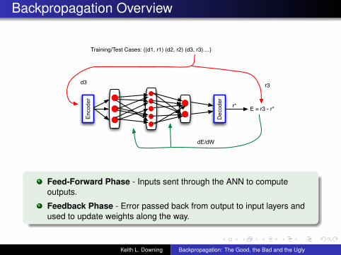
Training/Test Cases: {(d1, r1) (d2, r2) (d3, r3)....}

dE/dW

Feed-Forward Phase - Inputs sent through the ANN to computeoutputs.

Feedback Phase - Error passed back from output to input layers andused to update weights along the way.


Training -vs- Testing

Training

Test

Cases

Neural Net

N times, with learning

1 time, without learning

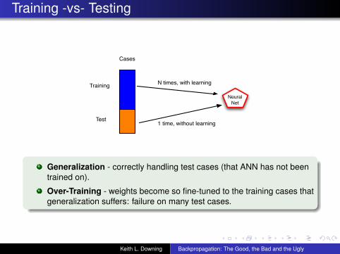
Generalization - correctly handling test cases (that ANN has not beentrained on).

Over-Training - weights become so fine-tuned to the training cases thatgeneralization suffers: failure on many test cases.


Widrow-Hoff (a.k.a. Delta) Rule

0

1

0

Y

S

1

2 3

w

X

Y

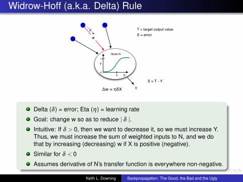
T = target output value δ = error

δ = T - Y

Δw = ηδX

Node N

Delta (δ ) = error; Eta (η) = learning rate

Goal: change w so as to reduce | δ |.Intuitive: If δ > 0, then we want to decrease it, so we must increase Y.Thus, we must increase the sum of weighted inputs to N, and we dothat by increasing (decreasing) w if X is positive (negative).

Similar for δ < 0

Assumes derivative of N’s transfer function is everywhere non-negative.


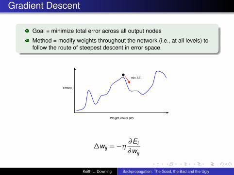
Gradient Descent

Goal = minimize total error across all output nodes

Method = modify weights throughout the network (i.e., at all levels) tofollow the route of steepest descent in error space.

Error(E)

Weight Vector (W)

min ΔE

∆wij =−η∂Ei

∂wij


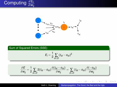
Computing ∂Ei∂wij

i

1

oid

tid

Eid

x1dwi1

n

xndwin

sumid

fT

Sum of Squared Errors (SSE)

Ei =12 ∑

d∈D(tid −oid )2

∂E∂wij

=12 ∑

d∈D2(tid −oid )

∂ (tid −oid )

∂wij= ∑

d∈D(tid −oid )

∂ (−oid )

∂wij


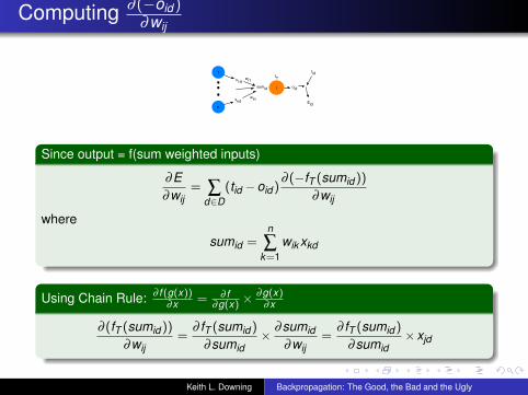
Computing ∂ (−oid )∂wij

i

1

oid

tid

Eid

x1dwi1

n

xndwin

sumid

fT

Since output = f(sum weighted inputs)

∂E∂wij

= ∑d∈D

(tid −oid )∂ (−fT (sumid ))

∂wij

where

sumid =n

∑k=1

wik xkd

Using Chain Rule: ∂ f (g(x))∂x = ∂ f

∂g(x) ×∂g(x)

∂x

∂ (fT (sumid ))

∂wij=

∂ fT (sumid )

∂sumid× ∂sumid

∂wij=

∂ fT (sumid )

∂sumid×xjd


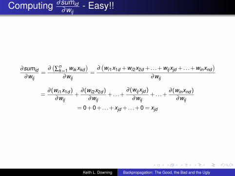
Computing ∂sumid∂wij

- Easy!!

∂sumid∂wij

=∂(∑

nk=1 wik xkd

)∂wij

=∂(wi1x1d + wi2x2d + . . .+ wijxjd + . . .+ winxnd

)∂wij

=∂ (wi1x1d )

∂wij+

∂ (wi2x2d )

∂wij+ . . .+

∂ (wijxjd )

∂wij+ . . .+

∂ (winxnd )

∂wij

= 0 + 0 + . . .+ xjd + . . .+ 0 = xjd


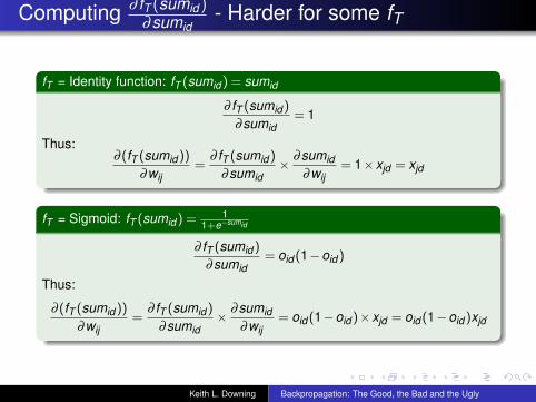
Computing ∂ fT (sumid )∂sumid

- Harder for some fT

fT = Identity function: fT (sumid ) = sumid

∂ fT (sumid )

∂sumid= 1

Thus:∂ (fT (sumid ))

∂wij=

∂ fT (sumid )

∂sumid× ∂sumid

∂wij= 1×xjd = xjd

fT = Sigmoid: fT (sumid ) = 11+e−sumid

∂ fT (sumid )

∂sumid= oid (1−oid )

Thus:

∂ (fT (sumid ))

∂wij=

∂ fT (sumid )

∂sumid× ∂sumid

∂wij= oid (1−oid )×xjd = oid (1−oid )xjd


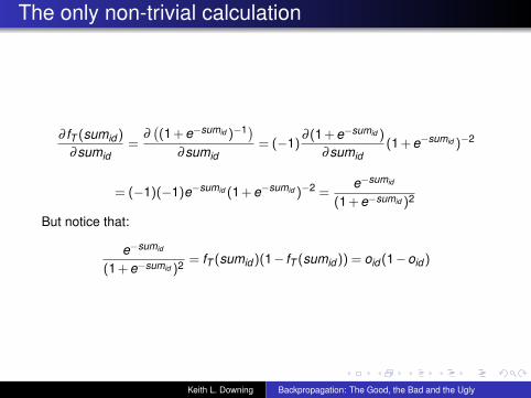
The only non-trivial calculation

∂ fT (sumid )

∂sumid=

∂((1 + e−sumid )−1)

∂sumid= (−1)

∂ (1 + e−sumid )

∂sumid(1 + e−sumid )−2

= (−1)(−1)e−sumid (1 + e−sumid )−2 =e−sumid

(1 + e−sumid )2

But notice that:

e−sumid

(1 + e−sumid )2 = fT (sumid )(1− fT (sumid )) = oid (1−oid )


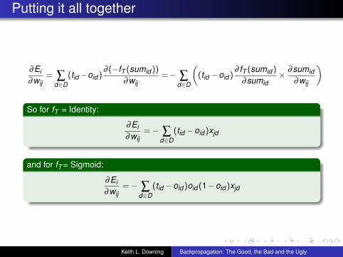
Putting it all together

∂Ei∂wij

= ∑d∈D

(tid−oid )∂ (−fT (sumid ))

∂wij=− ∑

d∈D

((tid −oid )

∂ fT (sumid )

∂sumid× ∂sumid

∂wij

)

So for fT = Identity:

∂Ei∂wij

=− ∑d∈D

(tid −oid )xjd

and for fT = Sigmoid:

∂Ei∂wij

=− ∑d∈D

(tid −oid )oid (1−oid )xjd


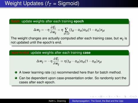
Weight Updates (fT = Sigmoid)

Batch: update weights after each training epoch

∆wij =−η∂Ei∂wij

= η ∑d∈D

(tid −oid )oid (1−oid )xjd

The weight changes are actually computed after each training case, but wij isnot updated until the epoch’s end.

Incremental: update weights after each training case

∆wij =−η∂Ei∂wij

= η(tid −oid )oid (1−oid )xjd

A lower learning rate (η) recommended here than for batch method.

Can be dependent upon case-presentation order. So randomly sort thecases after each epoch.


Backpropagation in Multi-Layered Neural Networks

1

n

jsumjdojd

wnj

w1j

d(ojd)

d(sumjd)

d(sumnd)

d(ojd)

d(sum1d)

d(ojd)

d(Ed)

d(sum1d)

d(Ed)

d(sumnd)

Ed

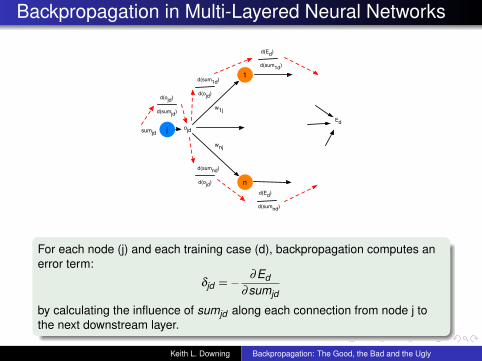
For each node (j) and each training case (d), backpropagation computes anerror term:

δjd =− ∂Ed∂sumjd

by calculating the influence of sumjd along each connection from node j tothe next downstream layer.


Computing δjd

1

n

jsumjdojd

wnj

w1j

d(ojd)

d(sumjd)

d(sumnd)

d(ojd)

d(sum1d)

d(ojd)

d(Ed)

d(sum1d)

d(Ed)

d(sumnd)

Ed

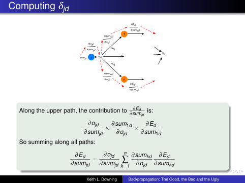
Along the upper path, the contribution to ∂Ed∂sumjd

is:

∂ojd

∂sumjd× ∂sum1d

∂ojd× ∂Ed

∂sum1d

So summing along all paths:

∂Ed∂sumjd

=∂ojd

∂sumjd

n

∑k=1

∂sumkd∂ojd

∂Ed∂sumkd


Computing δjd

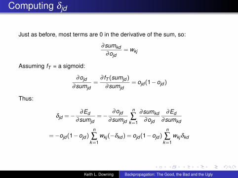
Just as before, most terms are 0 in the derivative of the sum, so:

∂sumkd∂ojd

= wkj

Assuming fT = a sigmoid:

∂ojd

∂sumjd=

∂ fT (sumjd )

∂sumjd= ojd (1−ojd )

Thus:

δjd =− ∂Ed∂sumjd

=−∂ojd

∂sumjd

n

∑k=1

∂sumkd∂ojd

∂Ed∂sumkd

=−ojd (1−ojd )n

∑k=1

wkj (−δkd ) = ojd (1−ojd )n

∑k=1

wkj δkd


Computing δjd

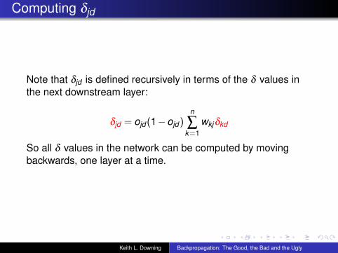
Note that δjd is defined recursively in terms of the δ values inthe next downstream layer:

δjd = ojd (1−ojd )n

∑k=1

wkjδkd

So all δ values in the network can be computed by movingbackwards, one layer at a time.


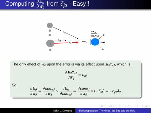
Computing ∂Ed∂wij

from δjd - Easy!!

j iwij

d(Ed)

d(sumid)

1

ojd

wi1

sumid

The only effect of wij upon the error is via its effect upon sumid , which is:

∂sumid∂wij

= ojd

So:∂Ed∂wij

=∂sumid

∂wij× ∂Ed

∂sumid=

∂sumid∂wij

× (−δid ) =−ojd δid


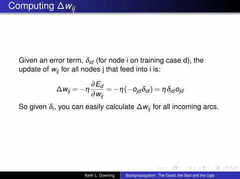
Computing ∆wij

Given an error term, δid (for node i on training case d), theupdate of wij for all nodes j that feed into i is:

∆wij =−η∂Ed

∂wij=−η(−ojd δid ) = ηδidojd

So given δi , you can easily calculate ∆wij for all incoming arcs.


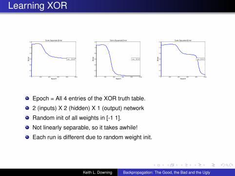
Learning XOR

0 200 400 600 800 1000

Epoch

0.0

0.2

0.4

0.6

0.8

1.0

1.2

Err

or

Sum-Squared-Error

Error

0 200 400 600 800 1000

Epoch

0.0

0.2

0.4

0.6

0.8

1.0

1.2

Err

or

Sum-Squared-Error

Error

0 200 400 600 800 1000

Epoch

0.0

0.2

0.4

0.6

0.8

1.0

1.2

Err

or

Sum-Squared-Error

Error

Epoch = All 4 entries of the XOR truth table.

2 (inputs) X 2 (hidden) X 1 (output) network

Random init of all weights in [-1 1].

Not linearly separable, so it takes awhile!

Each run is different due to random weight init.


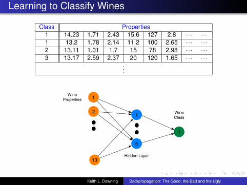
Learning to Classify Wines

Class Properties1 14.23 1.71 2.43 15.6 127 2.8 · · · · · ·1 13.2 1.78 2.14 11.2 100 2.65 · · · · · ·2 13.11 1.01 1.7 15 78 2.98 · · · · · ·3 13.17 2.59 2.37 20 120 1.65 · · · · · ·

...

1

1

5

2

13

1

WineProperties

WineClass

Hidden Layer


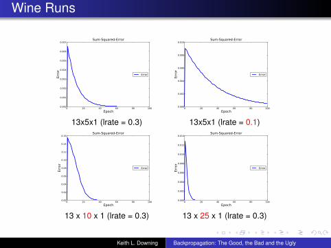
Wine Runs

0 20 40 60 80 100

Epoch

0.000

0.001

0.002

0.003

0.004

0.005

0.006

0.007

Err

or

Sum-Squared-Error

Error

0 20 40 60 80 100

Epoch

0.000

0.002

0.004

0.006

0.008

0.010

Err

or

Sum-Squared-Error

Error

13x5x1 (lrate = 0.3) 13x5x1 (lrate = 0.1)

0 20 40 60 80 100

Epoch

0.00

0.02

0.04

0.06

0.08

0.10

0.12

0.14

0.16

Err

or

Sum-Squared-Error

Error

0 20 40 60 80 100

Epoch

0.000

0.002

0.004

0.006

0.008

0.010

0.012

0.014

Err

or

Sum-Squared-Error

Error

13 x 10 x 1 (lrate = 0.3) 13 x 25 x 1 (lrate = 0.3)


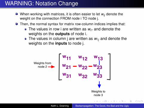
WARNING: Notation Change

When working with matrices, it is often easier to let wij denote theweight on the connection FROM node i TO node j.

Then, the normal syntax for matrix row-column indices implies that:The values in row i are written as wi? and denote theweights on the outputs of node i.The values in column j are written as w?j and denote theweights on the inputs to node j.

w11w21w31

w12w22w32

w13w23w33

Weights from node 2

Weights to node 3


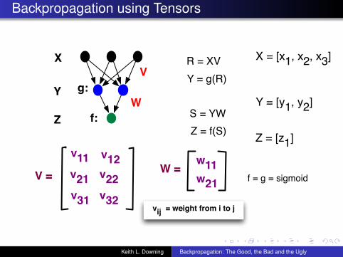
Backpropagation using Tensors

X

Y

Z f:

g:V

W

X = [x1, x2, x3]

Y = [y1, y2]

Z = [z1]v11v21v31

v12v22v32

V = w11w21

W =

R = XV

S = YW

Y = g(R)

Z = f(S)

f = g = sigmoid

vij = weight from i to j


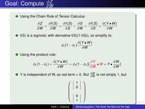
Goal: Compute ∂Z∂W

Using the Chain Rule of Tensor Calculus:

∂Z∂W

=∂ f (S)

∂W=

∂ f (S)

∂S× ∂S

∂W=

∂ f (S)

∂S× ∂ (Y •W )

∂W

f(S) is a sigmoid, with derivative f(S)(1-f(S)), so simplify to:

z1(1−z1)∂ (Y •W )

∂W

Using the product rule:

z1(1−z1)× ∂ (Y •W )

∂W= z1(1−z1)[

∂Y∂W•W + Y • ∂W

∂W]

Y is independent of W, so red term = 0. But ∂W∂W is not simply 1, but:

∣∣∣∣ 10

∣∣∣∣∣∣∣∣ 0

1

∣∣∣∣


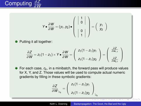
Computing ∂Z∂W

Y • ∂W∂W

= (y1,y2)•

∣∣∣∣ 1

0

∣∣∣∣∣∣∣∣ 0

1

∣∣∣∣

=

(y1y2

)

Putting it all together:

∂Z∂W

= z1(1−z1)×Y • ∂W∂W

=

z1(1−z1)y1

z1(1−z1)y2

=

∂Z

∂w1,1

∂Z∂w2,1

For each case, ck , in a minibatch, the forward pass will produce valuesfor X, Y, and Z. Those values will be used to compute actual numericgradients by filling in these symbolic gradients:

∂Z∂W |ck

=

z1(1−z1)y1

z1(1−z1)y2

|ck


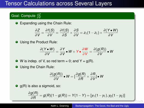
Tensor Calculations across Several Layers

Goal: Compute ∂Z∂V

Expanding using the Chain Rule:

∂Z∂V

=∂ f (S)

∂V=

∂ f (S)

∂S× ∂S

∂V= z1(1−z1)× ∂ (Y •W )

∂V

Using the Product Rule:

∂ (Y •W )

∂V=

∂Y∂V•W + Y • ∂W

∂V=

∂ (g(R))

∂V•W

W is indep. of V, so red term = 0; and Y = g(R).

Using the Chain Rule:

∂ (g(R))

∂V•W = [

∂g(R)

∂R× ∂R

∂V]•W

g(R) is also a sigmoid, so:

∂g(R)

∂R= g(R)(1−g(R)) = Y (1−Y ) = [y1(1−y1),y2(1−y2)]


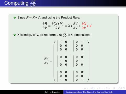
Computing ∂Z∂V

Since R = X •V , and using the Product Rule:

∂R∂V

=∂ (X •V )

∂V= X • ∂V

∂V+

∂X∂V•V

X is indep. of V, so red term = 0; ∂V∂V is 4-dimensional:

∂V∂V

=

∣∣∣∣∣∣1 00 00 0

∣∣∣∣∣∣∣∣∣∣∣∣

0 10 00 0

∣∣∣∣∣∣∣∣∣∣∣∣

0 01 00 0

∣∣∣∣∣∣∣∣∣∣∣∣

0 00 10 0

∣∣∣∣∣∣∣∣∣∣∣∣

0 00 01 0

∣∣∣∣∣∣∣∣∣∣∣∣

0 00 00 1

∣∣∣∣∣∣


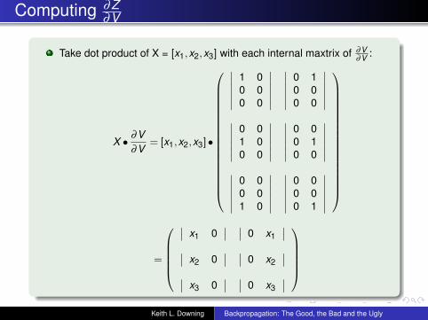
Computing ∂Z∂V

Take dot product of X = [x1,x2,x3] with each internal maxtrix of ∂V∂V :

X • ∂V∂V

= [x1,x2,x3]•

∣∣∣∣∣∣1 00 00 0

∣∣∣∣∣∣∣∣∣∣∣∣

0 10 00 0

∣∣∣∣∣∣∣∣∣∣∣∣

0 01 00 0

∣∣∣∣∣∣∣∣∣∣∣∣

0 00 10 0

∣∣∣∣∣∣∣∣∣∣∣∣

0 00 01 0

∣∣∣∣∣∣∣∣∣∣∣∣

0 00 00 1

∣∣∣∣∣∣

=

∣∣ x1 0

∣∣ ∣∣ 0 x1∣∣∣∣ x2 0

∣∣ ∣∣ 0 x2∣∣∣∣ x3 0

∣∣ ∣∣ 0 x3∣∣


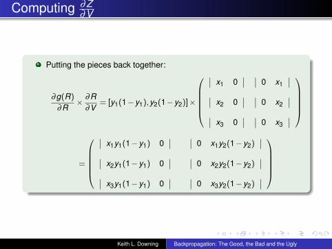
Computing ∂Z∂V

Putting the pieces back together:

∂g(R)

∂R× ∂R

∂V= [y1(1−y1),y2(1−y2)]×

∣∣ x1 0

∣∣ ∣∣ 0 x1∣∣∣∣ x2 0

∣∣ ∣∣ 0 x2∣∣∣∣ x3 0

∣∣ ∣∣ 0 x3∣∣

=

∣∣ x1y1(1−y1) 0

∣∣ ∣∣ 0 x1y2(1−y2)∣∣∣∣ x2y1(1−y1) 0

∣∣ ∣∣ 0 x2y2(1−y2)∣∣∣∣ x3y1(1−y1) 0

∣∣ ∣∣ 0 x3y2(1−y2)∣∣


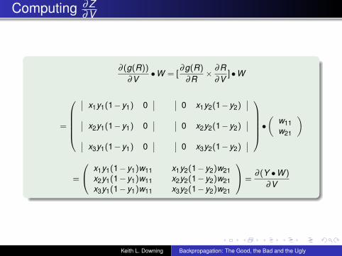
Computing ∂Z∂V

∂ (g(R))

∂V•W = [

∂g(R)

∂R× ∂R

∂V]•W

=

∣∣ x1y1(1−y1) 0

∣∣ ∣∣ 0 x1y2(1−y2)∣∣∣∣ x2y1(1−y1) 0

∣∣ ∣∣ 0 x2y2(1−y2)∣∣∣∣ x3y1(1−y1) 0

∣∣ ∣∣ 0 x3y2(1−y2)∣∣

•(

w11w21

)

=

x1y1(1−y1)w11 x1y2(1−y2)w21x2y1(1−y1)w11 x2y2(1−y2)w21x3y1(1−y1)w11 x3y2(1−y2)w21

=∂ (Y •W )

∂V


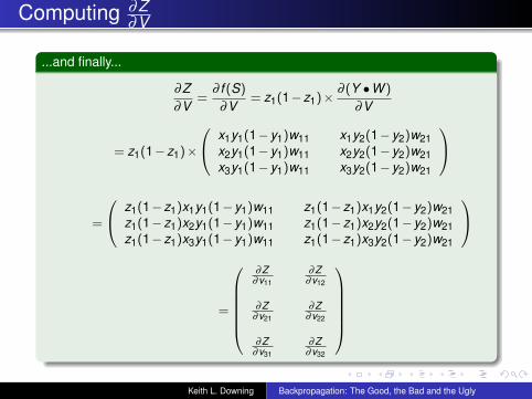
Computing ∂Z∂V

...and finally...

∂Z∂V

=∂ f (S)

∂V= z1(1−z1)× ∂ (Y •W )

∂V

= z1(1−z1)×

x1y1(1−y1)w11 x1y2(1−y2)w21x2y1(1−y1)w11 x2y2(1−y2)w21x3y1(1−y1)w11 x3y2(1−y2)w21

=

z1(1−z1)x1y1(1−y1)w11 z1(1−z1)x1y2(1−y2)w21z1(1−z1)x2y1(1−y1)w11 z1(1−z1)x2y2(1−y2)w21z1(1−z1)x3y1(1−y1)w11 z1(1−z1)x3y2(1−y2)w21

=

∂Z

∂v11

∂Z∂v12

∂Z∂v21

∂Z∂v22

∂Z∂v31

∂Z∂v32


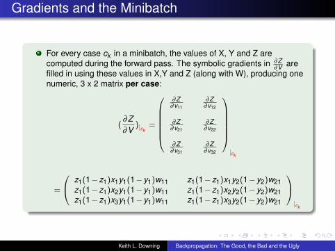
Gradients and the Minibatch

For every case ck in a minibatch, the values of X, Y and Z arecomputed during the forward pass. The symbolic gradients in ∂Z

∂V arefilled in using these values in X,Y and Z (along with W), producing onenumeric, 3 x 2 matrix per case:

(∂Z∂V

)|ck=

∂Z

∂v11

∂Z∂v12

∂Z∂v21

∂Z∂v22

∂Z∂v31

∂Z∂v32

|ck

=


|ck


Gradients and the Minibatch

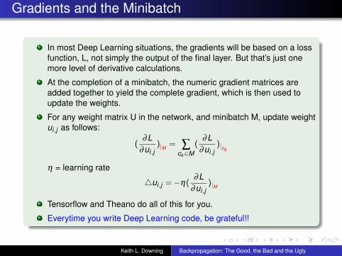
In most Deep Learning situations, the gradients will be based on a lossfunction, L, not simply the output of the final layer. But that’s just onemore level of derivative calculations.

At the completion of a minibatch, the numeric gradient matrices areadded together to yield the complete gradient, which is then used toupdate the weights.

For any weight matrix U in the network, and minibatch M, update weightui ,j as follows:

(∂L

∂ui ,j)|M = ∑

ck∈M(

∂L∂ui ,j

)|ck

η = learning rate

4ui ,j =−η(∂L

∂ui ,j)|M

Tensorflow and Theano do all of this for you.

Everytime you write Deep Learning code, be grateful!!


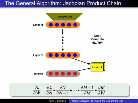
The General Algorithm: Jacobian Product Chain

Weights (W)

Targets

Layer N

Layer M

Loss (L)

Goal: Compute dL / dW

∂L∂W

=∂L∂N• ∂N

∂N−1• · · · • ∂M + 1

∂M• ∂M

∂W


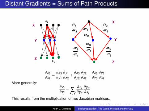
Distant Gradients = Sums of Path Products

X

Y

Z

X

Y

Z

X2

dZ3

dY1

dY2

dZ3

Z3

dY3

dX2dY2

dX2

dY1

dX2

dY3

dZ3

∂z3∂x2

=∂z3∂y1

∂y1∂x2

+∂z3∂y2

∂y2∂x2

+∂z3∂y3

∂y3∂x2

More generally:∂zi∂xj

= ∑k∈Y

∂zi∂yk

∂yk∂xj

This results from the multiplication of two Jacobian matrices.


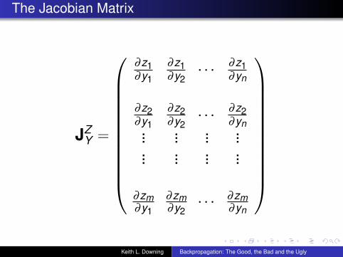
The Jacobian Matrix

JZY =

∂z1∂y1

∂z1∂y2· · · ∂z1

∂yn

∂z2∂y1

∂z2∂y2· · · ∂z2

∂yn... ... ... ...... ... ... ...

∂zm∂y1

∂zm∂y2· · · ∂zm

∂yn


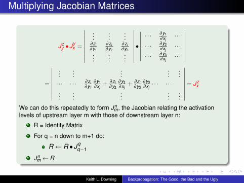
Multiplying Jacobian Matrices

Jzy •Jy

x =

∣∣∣∣∣∣∣∣∣...

......

∂zi∂y1

∂zi∂y2

∂zi∂y3

......

...

∣∣∣∣∣∣∣∣∣•∣∣∣∣∣∣∣∣· · · ∂y1

∂xj· · ·

· · · ∂y2∂xj

· · ·· · · ∂y3

∂xj· · ·

∣∣∣∣∣∣∣∣

=

∣∣∣∣∣∣∣∣∣...

......

......

· · · · · · ∂zi∂y1

∂y1∂xj

+ ∂zi∂y2

∂y2∂xj

+ ∂zi∂y3

∂y3∂xj· · · · · ·

......

......

...

∣∣∣∣∣∣∣∣∣= Jzx

We can do this repeatedly to form Jnm, the Jacobian relating the activation

levels of upstream layer m with those of downstream layer n:

R = Identity Matrix

For q = n down to m+1 do:

R← R •Jqq−1

Jnm← R


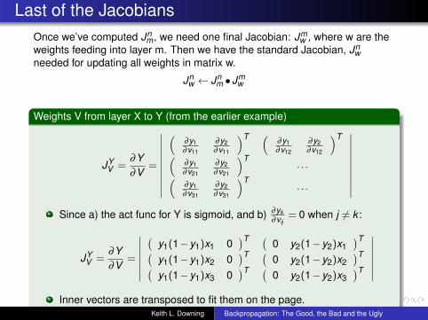
Last of the JacobiansOnce we’ve computed Jn

m, we need one final Jacobian: Jmw , where w are the

weights feeding into layer m. Then we have the standard Jacobian, Jnw

needed for updating all weights in matrix w.

Jnw ← Jn

m •Jmw

Weights V from layer X to Y (from the earlier example)

JYV =

∂Y∂V

=

∣∣∣∣∣∣∣∣∣∣

(∂y1∂v11

∂y2∂v11

)T (∂y1∂v12

∂y2∂v12

)T(∂y1∂v21

∂y2∂v21

)T· · ·(

∂y1∂v31

∂y2∂v31

)T· · ·

∣∣∣∣∣∣∣∣∣∣Since a) the act func for Y is sigmoid, and b) ∂yk

∂vij= 0 when j 6= k :

JYV =

∂Y∂V

=

∣∣∣∣∣∣∣(

y1(1−y1)x1 0)T (

0 y2(1−y2)x1)T(

y1(1−y1)x2 0)T (

0 y2(1−y2)x2)T(

y1(1−y1)x3 0)T (

0 y2(1−y2)x3)T

∣∣∣∣∣∣∣Inner vectors are transposed to fit them on the page.


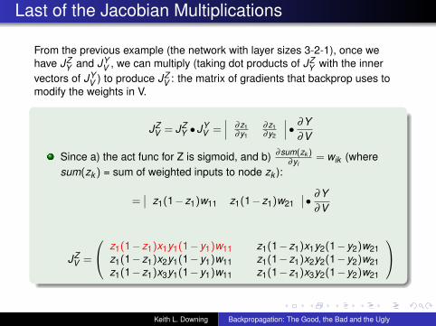
Last of the Jacobian Multiplications

From the previous example (the network with layer sizes 3-2-1), once wehave JZ

Y and JYV , we can multiply (taking dot products of JZ

Y with the innervectors of JY

V ) to produce JZV : the matrix of gradients that backprop uses to

modify the weights in V.

JZV = JZ

Y •JYV =

∣∣∣ ∂z1∂y1

∂z1∂y2

∣∣∣• ∂Y∂V

Since a) the act func for Z is sigmoid, and b) ∂sum(zk )∂yi

= wik (wheresum(zk ) = sum of weighted inputs to node zk ):

=∣∣ z1(1−z1)w11 z1(1−z1)w21

∣∣• ∂Y∂V

JZV =



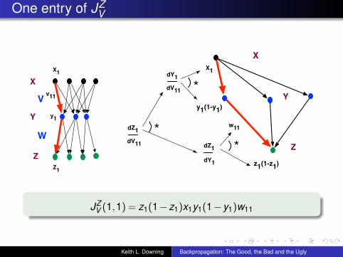
One entry of JZV

X

Y

Z

X1

Z1

V

W

v11

y1

X1

y1(1-y1)

w11

z1(1-z1)

dY1

dV11

dZ1

dY1

*

*

X

Y

Z

dZ1

dV11

*

JZV (1,1) = z1(1−z1)x1y1(1−y1)w11


First of the Jacobians

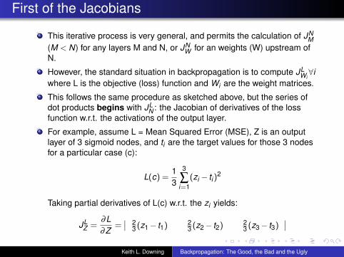
This iterative process is very general, and permits the calculation of JNM

(M < N) for any layers M and N, or JNW for an weights (W) upstream of

N.

However, the standard situation in backpropagation is to compute JLWi∀i

where L is the objective (loss) function and Wi are the weight matrices.

This follows the same procedure as sketched above, but the series ofdot products begins with JL

N : the Jacobian of derivatives of the lossfunction w.r.t. the activations of the output layer.

For example, assume L = Mean Squared Error (MSE), Z is an outputlayer of 3 sigmoid nodes, and ti are the target values for those 3 nodesfor a particular case (c):

L(c) =13

3

∑i=1

(zi − ti )2

Taking partial derivatives of L(c) w.r.t. the zi yields:

JLZ =

∂L∂Z

=∣∣ 2

3 (z1− t1) 23 (z2− t2) 2

3 (z3− t3)∣∣


First of the Jacobian Multiplications

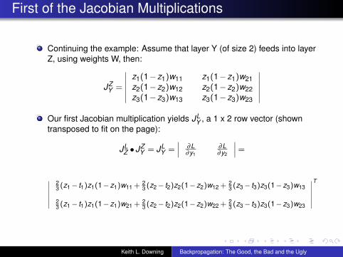
Continuing the example: Assume that layer Y (of size 2) feeds into layerZ, using weights W, then:

JZY =

∣∣∣∣∣∣z1(1−z1)w11 z1(1−z1)w21z2(1−z2)w12 z2(1−z2)w22z3(1−z3)w13 z3(1−z3)w23

∣∣∣∣∣∣Our first Jacobian multiplication yields JL

Y , a 1 x 2 row vector (showntransposed to fit on the page):

JLZ •JZ

Y = JLY =

∣∣∣ ∂L∂y1

∂L∂y2

∣∣∣=

∣∣∣∣∣∣23 (z1− t1)z1(1−z1)w11 +

23 (z2− t2)z2(1−z2)w12 +

23 (z3− t3)z3(1−z3)w13

23 (z1− t1)z1(1−z1)w21 +

23 (z2− t2)z2(1−z2)w22 +

23 (z3− t3)z3(1−z3)w23

∣∣∣∣∣∣T


Backpropagation with Tensors: The Big Picture

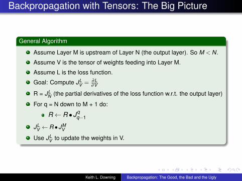
General Algorithm

Assume Layer M is upstream of Layer N (the output layer). So M < N.

Assume V is the tensor of weights feeding into Layer M.

Assume L is the loss function.

Goal: Compute JLV = ∂L

∂V

R = JLN (the partial derivatives of the loss function w.r.t. the output layer)

For q = N down to M + 1 do:

R← R •Jqq−1

JLV ← R •JM

V

Use JLV to update the weights in V.


Practical Tips

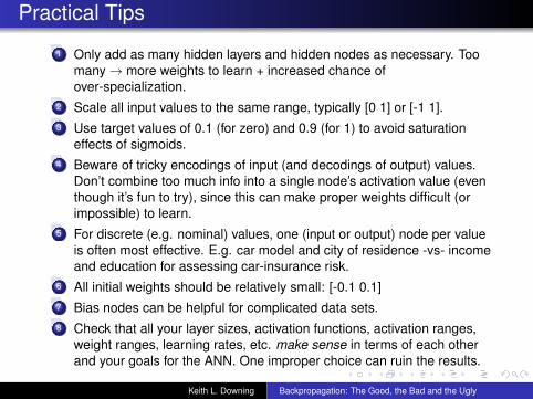
1 Only add as many hidden layers and hidden nodes as necessary. Toomany→ more weights to learn + increased chance ofover-specialization.

2 Scale all input values to the same range, typically [0 1] or [-1 1].3 Use target values of 0.1 (for zero) and 0.9 (for 1) to avoid saturation

effects of sigmoids.4 Beware of tricky encodings of input (and decodings of output) values.

Don’t combine too much info into a single node’s activation value (eventhough it’s fun to try), since this can make proper weights difficult (orimpossible) to learn.

5 For discrete (e.g. nominal) values, one (input or output) node per valueis often most effective. E.g. car model and city of residence -vs- incomeand education for assessing car-insurance risk.

6 All initial weights should be relatively small: [-0.1 0.1]7 Bias nodes can be helpful for complicated data sets.8 Check that all your layer sizes, activation functions, activation ranges,

weight ranges, learning rates, etc. make sense in terms of each otherand your goals for the ANN. One improper choice can ruin the results.


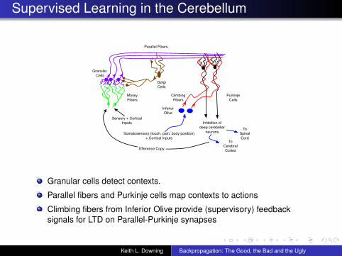
Supervised Learning in the Cerebellum

Parallel Fibers

Granular Cells

MossyFibers

ClimbingFibers

PurkinjeCells

InferiorOlive

Inhibition ofdeep cerebellar

neurons

To CerebralCortex

ToSpinalCord

Sensory + CorticalInputs

Somatosensory (touch, pain, body position) + Cortical Inputs

GolgiCells

Efference Copy

Granular cells detect contexts.

Parallel fibers and Purkinje cells map contexts to actions

Climbing fibers from Inferior Olive provide (supervisory) feedbacksignals for LTD on Parallel-Purkinje synapses


Documents

Backpropagation: The Good, the Bad and the Ugly · Keith L. Downing Backpropagation: The Good, the Bad and the Ugly. Practical Tips 1 Only add as many hidden layers and hidden nodes