A Vertical Representation for Parallel dEclat Algorithm in

Frequent Itemset Mining

by

Trieu Anh Tuan

Ritsumeikan University 2012

A Dissertation Submitted in Partial Fulfillment of the Requirements for Degree of

Master of Engineering

In the Department of Computer Science

1

Contents

Introduction..................................................................................................................................................5

1. Frequent Itemset Mining...............................................................................................................5

2. Objectives.......................................................................................................................................6

3. Contributions.................................................................................................................................6

4. Thesis Outline................................................................................................................................6

Background....................................................................................................................................................8

1. Problem Definition........................................................................................................................8

2. Downward Closed Property........................................................................................................10

3. Data Representation: Vertical and Horizontal Layout.............................................................10

4. Eclat Algorithm............................................................................................................................12

5. Diffset Format and dEclat Algorithm........................................................................................16

An Enhancement for Vertical Representation and Parallel dEclat..............................................................20

1. Combination of Tidset and Diffset Format................................................................................20

2. Sorting Tidsets and Diffsets........................................................................................................21

3. Coarse-grained Parallel Approach for dEclat...........................................................................22

4. Fine-grained Parallel Approach for dEclat...............................................................................23

Experiments.................................................................................................................................................31

1. Evaluate Effectiveness of The Enhancement for Vertical Representation..............................31

2. Evaluate Performance of The Two Parallel Approaches..........................................................36

Conclusion..................................................................................................................................................39

2

List of Figures

Figure 1 Horizontal and Vertical Layout......................................................................................11

Figure 2 Search Tree of The Item Base {a,b,c,d,e}.....................................................................14

Figure 3 Mining frequent Itemsets with Eclat...............................................................................16

Figure 4 Illustration of Diffset Format..........................................................................................17

Figure 5 How dEclat Works.........................................................................................................18

Figure 6 dEclat with Sorted diffsets/tidsets..................................................................................22

Figure 7 Coarse-grained Parallel Approach................................................................................23

Figure 8 Load Unbalancing Problem on Dataset Pumsb*...........................................................23

Figure 9 Initial database size at various values of minimum support in different formats...........34

Figure 10 Average set size of com-Eclat and sorting-dEclat at various values of minimum

support.........................................................................................................................................34

Figure 11 Running time of com-Eclat and sorting-dEclat at various values of minimum support35

Figure 12 Load Unbalancing Problem in Coarse-Grained Approach..........................................37

Figure 13 Running time of coarse-dEclat and fine-dEclat on different datasets.........................38

3

List of Tables

Table 1: A Transaction Database with 3 Transactions from an Item Base with 6 Items...............9

Table 2 Database Characteristics...............................................................................................31

Table 3 The average set size of dEclat and sorting-dEclat at various values of minimum support

.....................................................................................................................................................32

Table 4 The running time (in seconds) of dEclat and sorting-dEclat at various values of

minimum support.........................................................................................................................33

4

Chapter 1

Introduction

1. Frequent Itemset Mining

Finding frequent itemsets or patterns has a strong and long-standing tradition in data

mining. It is a fundamental part of many data mining applications including market basket

analysis, web link analysis, genome analysis and molecular fragment mining.

Since its introduction by Agrawal et al [1] , it has received a great deal of attention and

various efficient and sophisticated algorithms have been proposed to do frequent itemset

mining. Among the best-known algorithms are Apriori, Eclat and FP-Growth.

The Apriori algorithm [2] uses a breadth-first search and the downward closure property,

in which any superset of an infrequent itemset is infrequent, to prune the search tree. Apriori

usually adopts a horizontal layout to represent the transaction database and the frequency of

an itemset is computed by counting its occurrence in each transaction.

FP-Growth [3] employs a divide-and-conquer strategy and a FP-tree data structure to

achieve a condensed representation of the transaction database. It is currently one of the

fastest algorithms for frequent pattern mining.

Eclat [4] takes a depth-first search and adopts a vertical layout to represent databases, in

which each item is represented by a set of transaction IDs (called a tidset) whose transactions

contain the item. Tidset of an itemset is generated by intersecting tidsets of its items. Because

of the depth-first search, it is difficult to utilize the downward closure property like in

Apriori. However, using tidsets has an advantage that there is no need for counting support,

the support of an itemset is the size of the tidset representing it. The main operation of Eclat

is intersecting tidsets, thus the size of tidsets is one of main factors affecting the running time

and memory usage of Eclat. The bigger tidsets are, the more time and memory are needed.

5

Zaki and Gouda [5] proposed a new vertical data representation, called Diffset, and

introduced dEclat, an Eclat-based algorithm using diffset. Instead of using tidsets, they use

the difference of tidsets (called diffsets). Using diffsets has reduced drastically the set size

representing itemsets and thus operations on sets are much faster. dEclat had been shown to

achieve significant improvements in performance as well as memory usage over Eclat,

especially on dense databases [5]. However, when the dataset is sparse, diffset loses its

advantage over tidset. Therefore, Zaki and Gouda suggested using tidset format at the start

for sparse databases and then switching to diffset format later when a switching condition is

met.

2. ObjectivesThe objective of this thesis is to improve the performance of frequent itemset mining by

dEclat algorithm.

3. Contributions

This thesis has introduced an enhancement for dEclat algorithm through a new data

format to represent itemsets and by sorting diffset/tidsets of itemsets.

In addition, we also introduce a new parallel approach for dEclat algorithm, which can

address the problem of load unbalancing and better exploit power of clusters with many

nodes.

4. Thesis Outline

We begin in chapter 2 by formally defining the frequent itemset mining problem and

giving background on it. Then in chapter 3, we introduce an enhancement for the vertical

representation used in dEclat algorithm and a new parallel approach for dEclat. This chapter

is broken into four parts; the first part is about a new format to facilitate the counting support

of dEclat; the second part is about a direct improvement for dEclat by sorting its

diffsets/tidsets; the third part presents the original parallel approach of dEclat and shows its

disadvantages; then in the last part, we propose a new approach to address these

disadvantages.

6

In chapter 4, we show the results of our experiments and then we compare and analyze

the results. Finally, in chapter 5, we conclude and indicate in what manner we believe this

research could be extended.

7

Chapter 2

Background

1. Problem Definition

Let be B= {i1 , i2 ,…,im} a set of m items. This set is called the item base. Items may be

products, services, actions etc. A set X={i1 ,…, ik }⊆B is called an itemset or a k−itemset if it

contains k items.

A transaction over B is a couple T i=( tid , I ) where tid is the transaction identifier and I is

an itemset. A transaction T i=( tid , I ) is said to support an itemset X⊆B if X⊆ I .

A transaction database T is a set of transaction overB.

A tidset of an itemset X in T is defined as a set of transaction identifiers of transactions in

T that supportX .

t ( X )={tid|( tid , I )∈T , X⊆I }

Support of an itemset X in T is the cardinality of its tidset. In other word, support of X is

the number of transactions containing X inT .

¿ ( X )=¿ t ( X )∨¿

An itemset X is called frequent if its support is no less than a predefined minimum

support thresholdsmin , with 0<smin<¿T∨¿.

Definition 1.1. Given a transaction database T over an item base B and a minimal

support threshold, smin. The set of all frequent itemsets is denoted by:

F (T , smin)={X⊆B∨( X ) ≥ smin }

8

Definition 1.2 (Frequent Itemset Mining): Given a transaction database T and a

minimum support threshold,smin, the problem of finding all the frequent itemsets is called

frequent itemset mining problem, denoted by F (T , smin).

Definition 1.3 (Search Tree): The search tree of the frequent itemset mining problem is

the set of all possible itemsets over B and it contains exactly 2|B| different itemsets.

An example of a search tree of an item base with five items is showed in the page 14.

Definition 1.4 (Candidate Itemset): Given a transaction databaseT , a minimum support

threshold,smin, and an algorithm that computes F (T , smin), an itemset X is called a candidate if

the algorithm evaluates if X is frequent or not.

To demonstrate the frequent itemset mining problem, let consider the transaction database in

the table below:

Table 1: A Transaction Database with 3 Transactions from an Item Base with 6 Items

T 0 abc

T 1 adf

T 2 acde

The item base is {a ,b , c , d , e , f }and the search tree contains 26 itemsets. The transaction

database has three transactions. If smin is set at 2, then there are three frequent itemsets:

{a }, {d } , {a ,d } because there are at least two transactions containing them.

These frequent itemsets potentially imply new knowledge about the database transaction.

A naïve and straightforward approach to find frequent itemsets is firstly generate all possible

itemsets from the item base and then, for each itemset, count its support by going through all

transactions in the transaction database and checking if transactions contain itemsets. In fact,

9

many proposed algorithms based on this simple approach with some modification for

generating itemsets and/or counting support more efficiently.

Although, the problem of finding all frequent itemsets looks simple, it is quite difficult

for two primary reasons: the transaction database is typically massive and the set of all

possible itemsets grow exponentially with the number of items in the item base, therefore the

itemset generating process and counting process are time and memory intensive. In fact,

given a fixed size k, determining if there exists a set of k-itemsets that co-occur in a

transaction database s times was demonstrated to be a NP-complete problem [6].

2. Downward Closed Property

If the size of the item base is large, then the naïve approach to generate and count the

supports of all itemsets in the search tree cannot be done in a reasonable period of time.

Therefore, it is important to generate as few itemsets as possible since both generating

itemsets and counting their supports are time consuming. The property that most algorithms

exploit to trim down the search tree is that the support of an itemset cannot be larger than the

supports of its subsets.

Downward Closed Property: Given a transaction database T over an item base B, let

X ,Y ⊆B be two itemsets. Then,

X⊆Y ⇒( Y )≤ (X)

From this property, if an itemset is infrequent, then all of its supersets are infrequent as

well. Therefore, in algorithms that exploit this property, only candidates where all of its

subsets are frequent are generated and counted for supports.

3. Data Representation: Vertical and Horizontal Layout

To count supports of candidates, we need to go through transactions in the transaction

database and check if transactions contain candidates. Since the transaction database is

usually very large, it is not always possible to store them into main memory. Furthermore, to

check if a transaction containing an itemset is also a non-trivial task. So an important

consideration in frequent itemset mining algorithms is the representation of the transaction

10

database to facilitate the process of counting support. There are two layouts that algorithms

usually employ to represent transaction databases: horizontal and vertical layout.

In the horizontal layout, each transaction T i is represented as T i :(tid , I ) where tid is the

transaction identifier and I is an itemset containing items occurring in the transaction. The

initial transaction consists of all transactionsT i.

Figure 1 Horizontal and Vertical Layout

In the vertical layout, each item ik in the item base B is represented as ik : {ik ,t ( ik) } and the

initial transaction database consists of all items in the item base.

For both layouts, it is possible to use the bit format to encode tids [7] [8] and also a

combination of both layouts can be used [9].

To count the support of an itemset X using the horizontal layout, one has to go through

all transactions and check if transactions contain the itemset. Therefore, both the number of

transactions in the transaction database and the size of transactions account for the

consuming time of the support counting step.

When using the vertical layout, in the transaction database the support of an itemset is the

size of its tidset. To count the support of an itemsetX , firstly its tidset will be generated by

11

intersecting the tidsets of any two itemsetsY ,Z suchthat Y ∪Z=X. So

t ( X )=t (Y )∩t (Z ) ,whereY ∪Z=X , this could be easily deduced from the definition of

tidset .Then the support of X is the size of its tidset.

In algorithms that employ the vertical layout, 2−itemsetsare generated from the initial

transaction database and then next k−itemsetsare generated by from(k−1 )−itemsets. As the

size of itemsets increases, the size of their tidsets will decrease, using the vertical layout,

counting support is usually faster and using less memory than counting support when using

the horizontal layout [8].

4. Eclat Algorithm

Eclat is based on two main steps: candidate generation and pruning. In the candidate

generation step, each k-itemset candidate is generated from two frequent (k−1 )−itemsetsand

then its support is counted, if its support is lower than the threshold, then it will be discarded,

otherwise it is frequent itemsets and used to generate(k+1 )−itemsets. Since Eclat uses the

vertical layout, counting support is trivial. Candidate generation is indeed a search in the

search tree. This search is a depth-first search and it starts with frequent items in the item

base and then 2−itemsetsare reached from1−itemsets, 3−itemsetsare reached from

2−itemsets and so on.

Candidate Generation

An k−itemset is generated by taking union of two (k−1 )−itemsets which have (k−2)

items in common, the two (k-1)-itemsets are called parent itemsets of the k-itemset. Fox

example, {abc }={ab }∪{ac }, {ab} and {ac} are parent of {abc}. To avoid generate duplicate

itemsets, (k−1 )−itemsets are sorted in some order.

To generate all possible k−itemsetsfrom a set of (k-1)-itemsets sharing (k-2) items, we

just do unions of a (k−1 )−itemsetwith all (k−1 )−itemsets that stand behind it in the sorted

order, and this process takes place for all (k−1 )−itemsets except the last one. For example,

we have a set of 1−itemsets {a ,b , c , d , e }, which share 0 item; we could sort items in the

alphabet order; to generate all 2−itemsets, we take union of {a } with {b,c,d,e} to result 2-

12

itemsets {ab,ac,ad,ae}, then we take union of {b} with {c,d,e} to have {bc,bd,be}, similarly

we do this for {c} and {d}; finally, we get all possible

2−itemsets {ab ,ac ,ad ,ae ,bc ,bd ,be , cd , ce , de } ; to generate all possible 3-itemsets from

these 2-itemsets, we firstly have to divide these itemsets into groups, where each group has a

common item; in each group, we do union to generate possible 3-itemsets from that group,

then gathering all 3-itemsets generated from groups, we have all possible 3-itemsets from the

item base {a,b,c,d,e}.

Definition 4.1.(Equivalence Class and Prefix): We define an equivalence class of k-

itemsets in a search tree is a set of all k-itemset in that search tree and having (k-1) items in

common. This (k-1) common items is called the prefix of the equivalence class.

An equivalence class is denoted as E={(i¿¿1 , t (i1∪P )) ,…,(ik ,t (ik∪P ))∨P }¿ where

i1 ,…, ik∉ P are the distinguished items of itemsets and P is the prefix of the equivalence

class; each item is accompanied by the tidset of its represented itemset. Itemsets of the

equivalence class are {( i1∪P ) ,…, (ik∪P ) } , when generating a new itemset by joining two

itemsets of this equivalence class, we just need to join two distinguished items of the two

itemsets and then append the prefix P to the result. During this process, we also generate the

tidset of the new itemset by intersecting the two respective tidsets accompanying the two

distinguished items. It could be seen that joining two itemsets to generate a new one and

support counting have now become trivial. Intersecting tidsets is the only operation worth to

count here.

From the definition, we can see that the item base with 1-itemset is an equivalence class

with the prefix {} and this equivalence class is equal to the initial transaction database in

vertical layout. Given a prefix, we have only one equivalence class correspondingly.

Given an equivalence classE={(i¿¿1 , t (i1∪P )) ,…,(ik ,t (ik∪P ))∨P }¿ , if we consider

the set {i1 ,…,ik } as an item base, we will have a tree of itemsets over this item base and if we

append the prefix P to all itemsets in this new tree, we will have a set of all itemsets sharing

the prefix P in the search tree over the item base B (we shall call the search tree over the item

base B as the initial search tree). In other word, from this equivalence class, we could

13

generate a set of all itemsets sharing the prefix P and this set forms a sub tree of the initial

search tree.

Eclat starts with the prefix {} and the search tree is actually the initial search tree. To

divide the initial search tree, it picks the prefix {a}, generate the corresponding equivalence

class and does frequent itemset mining in the sub tree of all itemsets containing {a}, in this

sub tree it divides further into two sub trees by picking the prefix {ab}: the first sub tree

consists of all itemset containing {ab}, the other consists of all itemsets containing {a} but

not {b}, and this process is recursive until all itemsets in the initial search tree are visited.

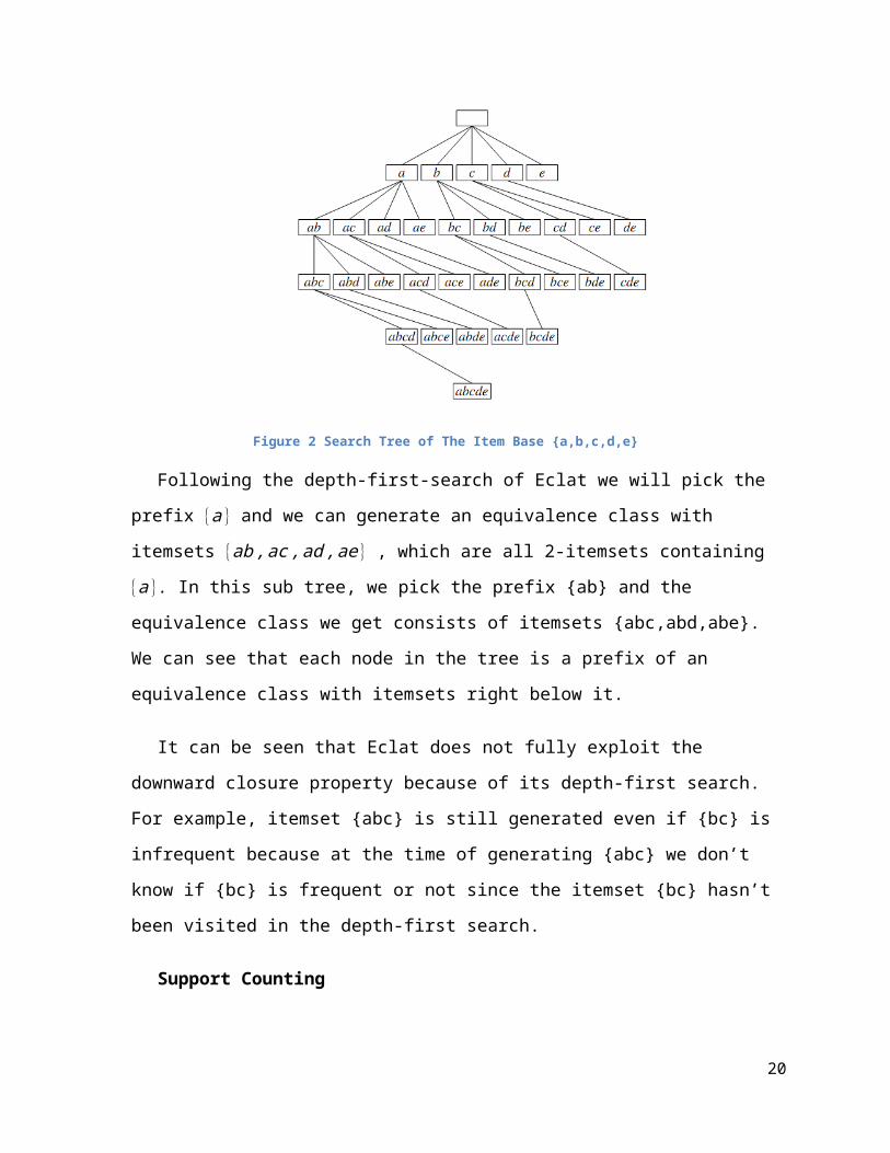
The search tree of an item base {a,b,c,d,e} is represented by the tree as below:

Figure 2 Search Tree of The Item Base {a,b,c,d,e}

Following the depth-first-search of Eclat we will pick the prefix {a } and we can generate

an equivalence class with itemsets {ab ,ac ,ad , ae } , which are all 2-itemsets containing {a }.

In this sub tree, we pick the prefix {ab} and the equivalence class we get consists of itemsets

{abc,abd,abe}. We can see that each node in the tree is a prefix of an equivalence class with

itemsets right below it.

It can be seen that Eclat does not fully exploit the downward closure property because of

its depth-first search. For example, itemset {abc} is still generated even if {bc} is infrequent

14

because at the time of generating {abc} we don’t know if {bc} is frequent or not since the

itemset {bc} hasn’t been visited in the depth-first search.

Support Counting

Whenever generating a candidate itemset, we also generate its tidset by intersecting the

tidsets of its parent. And the support of the candidate is the size of its tidset, so that support

counting is trivial and it is done simultaneously with candidate generating.

It can be seen that the main operation of Eclat is intersecting tidsets, thus the size of

tidsets is one of main factors affecting the running time and memory usage of Eclat. The

bigger tidsets are, the more time and memory are needed to mine all frequent itemsets.

The pseudo code for the Eclat algorithm is as follow:

Assumingthattheinitialtransactiondatabaseisinverticallayoutandrepresentedbyan

equivalenceclassEwithprefix{}.

Algorithm 1 Eclat

Input :E ((i1 ,t 1) ,… (in ,t n¿)∨P) , smin

Output :F (E , smin )1 : for all i joccuring∈E do

2: P≔P∪ i j//addi jtocreateanewprefix

3:init (E' )//initializeanewequivalenceclasswiththenewprefixP

4 : for all ikoccuring∈E such that k> j do

5 : t tmp=t j∩t k

6 : if |t tmp|≥ smin then

7 : E'≔E∪ (ik ,t tmp)

8 : F=F∪( ik∪P)

9 :end if

10:end for

11: if E' ≠{}then

12: Eclat (E' , smin)

13: end if

15

14:end for

Figure 3 Mining frequent Itemsets with Eclat

5. Diffset Format and dEclat Algorithm

Instead of using the common tids (transaction IDs) of the two parent itemsets to represent

an itemset, Zaki [5] represented an itemset by tids that appear in the tidset of its prefix but do

not appear in its tidset. This set of tids is called a diffset, the difference between the tidset of

the itemset and its prefix. Using diffset, the cardinality of sets representing itemsets is

reduced significantly and this results in faster intersection and less memory usage. Diffset

format was also demonstrated to increase the scalability of Apriori and Eclat when running in

parallel environments [10].

Formally, consider an equivalence class with prefix P and containing itemsets X, Y. Let’s

t(X) denote the tidset of X and d(X) denote the diffset of X. When using tidset format, we

will have t(PX) and t(PY) available in the equivalence class and to obtain t(PXY) we check

the cardinality of t (PX ) ∩t (PY )=t (PXY )

16

When using diffset format, we will have d(PX) instead of t(PX) and d ( PX )=t (P )− t(X),

the set of tids in t(P) but not in t(X). Similarly, we have d(PY) = t(P) – t(Y). So the support of

PX is not the size of its diffset. By the definition of d(PX), it can be seen that

|t (PX )|=|t (P )|−|t (P )−t ( X )|=|t (P )|−¿d ( PX )∨¿. In other word, ¿ ( PX )=(P)−¿d ( PX )∨¿. This

formula is illustrated by the figure below.

Figure 4 Illustration of Diffset Format

Now suppose that we are given d(PX) and d(PY), how can we calculate sup(PXY) and

generate d(PXY)? We already know that sup(PXY) = sup(PX) - |d(PXY)|. There after

generating d(PXY), we will have sup(PXY). Formally:

d(PXY) = t(PX) – t(PXY)

= t(PX) – t(PY)

= (t(P) – t(PY)) – (t(P) – t(PX))

= d(PY) – d(PX).

From this formula, given d(PX) and d(PY) we could generate d(PXY) and sup(PXY).

17

To use diffset format, the initial transaction database in vertical layout is firstly converted

to diffset format in which diffset of items are sets of tids whose transactions do not contain

items. This is deduced from the definition of diffset, the initial transaction database in

vertical layout is an equivalence with the prefix P={}, so the tidset of P includes all tids, all

transactions contain P, and the diffset of an item iis d (i )=t (P )−t(i), this is a set of tids

whose transactions do not contain i. From this initial equivalence class, we could generate all

itemsets with their diffsets and supports.

When Eclat uses the diffset format, it is called dEclat algorithm. And dEclat is different

from Eclat in the step 5, instead of generating a new tidset, a new diffset is generated.

Furthermore, we also need to store support of itemsets in equivalence class to facilitate

calculating supports of new itemsets.

Figure 5 How dEclat Works

The Switching Condition

The purpose of using diffset is to reduce the cardinality of sets representing itemsets.

However, it could be seen that cardinality of the diffset of an itemset is not always smaller

than the cardinality of the tidset of the itemset.

18

Therefore, when the size of d(PXY) is larger than the size of t(PXY), the usage of diffset

should be delayed. Theoretically, it is better to switch to the diffset format when the support

of PXY is at least half the support of PX . This is the switching condition for one tidset, for a

conditional database the average support could be used instead or the number of tidsets in the

equivalence class satisfying the switching condition could be took into consideration. In

either case, an equivalence class could be switched to diffset format even though it may

contain tidsets which do not satisfy the switching condition. Therefore, it is better to switch

only tidsets satisfying the switching condition but it may lead to the existence of both tidsets

and diffsets in an equivalence class.

We will show that tidset and diffset format can be used together to generate new diffsets

and calculate support of new itemsets. This combination can reduce the average set size of

sets representing itemsets and speed up the intersection.

19

Chapter 3

An Enhancement for Vertical Representation and

Parallel dEclat

1. Combination of Tidset and Diffset Format

As pointed out above, when switching an equivalence class from tidset format to diffset

format, there are tidsets which do not satisfy the switching condition and thus those tidsets

should be stored in tidset format instead of converting them to diffset format.

That means there are both tidset format and diffset format in an equivalence class and

intersection between an itemset in tidset format and an itemset in diffset format will occur.

However a tidset intersecting a diffset results a diffset as described below.

t ( PX ) ∩d (PY )= (t(P)∩t(X ))∩ (t (P)−t (Y ))

¿ (t (P)∩t (X ))−( t(P)∩t(X)∩t (Y ))

¿ t (PX )−t (PXY )

¿d (PXY )

For a given equivalence class with prefix P consisting of itemsets X i in some order, one

performs intersection of P X i with all P X j with j>i to obtain a new equivalence class with

prefix P X i and frequent itemsets X i X j . P X i and P X j could be in either tidset or diffset

format. If P X i is in diffset format and P X j is in tidset format, d (P X i )∩t (P X j )=d (P X j X i)

20

which belongs to the equivalence class of prefixP X j, not P X i as expected. That is to say, in

order to do intersection between itemsets in diffset format and itemsets in tidset format to

produce new equivalence classes properly, itemsets in tidset format must stand before

itemsets in diffset format in the order of their equivalence class. That can be achieved by

swapping itemsets in diffset and tidset format, a process which has the complexity O(n)

where n is the number of itemsets of the equivalence class.

Converting From Tidset To Diffset

Since d(PXY) = t(PX) - t(PY) and t(PXY) = t(PX) ∩ t(PY) so both d(PXY) and t(PXY)

can be generated concurrently from the two tidsets. Thus, the shorter one will be returned as

the result. There is no need to consider the switching condition and there is also no

conversion of tidset to diffset format.

2. Sorting Tidsets and Diffsets

Since sup(PXY)=sup(PX)-|d(PXY)|=sup(PY)-|d(PYX)| , both d(PXY) and d(PYX)

could be used to calculate sup(PXY). Therefore, the smaller one of the two should be used to

calculate sup(PXY) to reduce the memory usage and processing time. Because d(PXY)=

d(PY)-d(PX) and d(PYX)=d(PX)-d(PY), if d(PX) is smaller than d(PY) then d(PYX) is

smaller than d(PXY). It should be noted that because in an equivalence class of prefix P, one

performs intersection of P X i with all P X j with j>i to obtain a new equivalence class of the

prefix X i , so only d (P X i X j), where j>i exist. Similarly, if PX stands before PY in the order

of their equivalence class, d(PXY) will exist and if PX stands behind PY in the order of their

equivalence class, d(PYX) will exist. To obtain the smaller between d(PXY) and d(PYX), the

bigger of d(PX) and d(PY) must stand before the smaller one in the order of their equivalence

class. In general, diffsets in a equivalence class should be sorted in descending order

according to size to generate new itemsets represented by diffsets with smaller sizes.

The reverse order holds for tidsets. While t(PXY) does not depend on the order of t(PX)

and t(PY), d(PXY) depends on the order. As d(PXY)=t(PX)-t(PY) , if t(PX) is smaller than

t(PY), then d(PXY) is smaller than d(PYX). Thus it is desirable that tidsets are sorted in

ascending order according to their size.

21

Even though the sorting helps to produce diffsets in smaller sizes, there is a cost for

sorting. Our observation is that the size of equivalence class is relatively small (always less

than the size of the item base) and this size also reduces quickly as the search goes deeper in

the recursion process. Our experiments showed that the benefit of sorting outweighs the cost

of sorting and the sorting significantly reduces the running time and memory usage.

Figure 6 dEclat with Sorted diffsets/tidsets

3. Coarse-grained Parallel Approach for dEclat

The first parallel approach for Eclat was proposed by Zaki et al [11]. The basic idea is

that the search tree could be divided into sub trees of equivalence classes. And since

generating itemsets in sub trees of equivalence classes is independent from each other, we

could do frequent itemset mining in sub trees of equivalence classes in parallel.

22

So the straightforward approach to parallelize dEclat is to consider each equivalence class

as a job. And we can distribute jobs to different nodes and nodes could work on jobs without

any synchronization.

Figure 7 Coarse-grained Parallel Approach

23

This seems a perfect parallel scheme. However, the workloads here are not equal and we

may encounter the problem of load unbalancing. Experiments showed that for some datasets,

the processing times for their equivalence classes are extremely different. In these cases,

even if we add more nodes into our system, we cannot improve the overall performance.

4 8 12 16 20 240

100

200

300

400

500

600

Difference of the running time of the earliest and latest nodes

Earliest NodeLatest Node

Number of nodes

Runn

ing

time

in se

cond

s

Figure 8 Load Unbalancing Problem on Dataset Pumsb*

4. Fine-grained Parallel Approach for dEclat

The parallel approach above could be called the coarse-grained approach since its jobs

are fairly large. To address the problem of load unbalancing in the coarse-grained approach,

this thesis proposes a fine-grained approach in which equivalence classes are dynamically

divided into smaller jobs.

The idea is that instead of dividing job only at first level (dividing the initial equivalence

class), we can continuously divide equivalence classes whenever there is a free node and the

current equivalence class is relatively large. Each itemset in an equivalence class is a prefix

of a new equivalence class, so the search tree of an equivalence class consists of several sub

trees and mining in these trees is independent from each other.

However, the size of equivalence classes and the size of tidsets/diffsets of their itemsets

are unpredictable, so it is impossible to divide equivalence classes into equal jobs. Since the

size of tidsets/diffsets is the main factor contributing to the load of jobs, simple load

24

estimation for a job is summation of all the size of all possible tidsets/diffsets in the tree of

the equivalence class. This estimation is used to decide if the job should be divided further.

The job division strategy is that if a node is processing a job with load estimation over

some predefined threshold, this node shall be called an overload node, then it will ask the

master node for a free node, if there is a free node available, then the master node will inform

the overload node and the free node, and then the two node will communicate to transfer job

from the overload node to the free node.

To reduce the cost of communication for asking master node for free node, especially

when the load unbalancing problem is not serious, nodes should not ask master node for free

node until the first free node is available.

Job Load Estimation

Since we cannot predict if any candidate itemset is discarded in the next level of the

depth-first search, we can assume that there is no infrequent itemsets in the next levels of the

depth-first search. In addition, the size of tidsets/diffsets of itemsets in the next levels is

unpredictable, but we are sure that this size cannot be larger than the size of the tidset/diffset

of its prefix. Therefore, an upper bound for the load of an equivalence class is summation of

the sizes of tidsets/diffsets of all possible itemsets in the search tree of the equivalence class.

25

The first step in job load estimation is to calculate the number of all possible itemsets and

then multiply it with the size of the tidset/diffset of the prefix.

Given an equivalence classE((i1 , d1),… (in , dn¿ )∨P), we want to calculate the number of

all possible itemsets in the search tree of equivalence classes with prefixesP ikwhere k=1…n

. Let f (Pik ) be the number of possible itemsets in the search tree of the equivalence class

with prefix P ik. From the search tree, it could be seen that:

f (P in )=1

f (P in−1 )=f (Pin )+1=2∗f (P in)

f (P in−2 )= f (Pin−1 )+ f (P in )+1=2∗f (Pin−1)

….

f (P i1 )=2∗f (P i2 )

From here we could calculate the number of possible itemsets in search trees of

equivalence classes recursively. And then the estimated job load of a job with prefix P ik is

f (P ik )∗|d (Pik )|∨f (Pik )∗¿ t (P ik)∨¿.

Parallelization Scheme

There is a master node, which acts as a coordinator; it is in charge of assigning

equivalence classes in the initial equivalence class to slave nodes. When a node has finish an

equivalence class from the initial equivalence class, it will ask master node for another one, if

there is no more equivalence class in the initial equivalence class, the node will become idle

and it is called a free node. The master will keep a list of free nodes. When the master node

cannot return an equivalence class in the initial equivalence class to a slave node, the slave

node will be added into the list of free nodes.

When a slave node has to process an equivalence, whose estimation load is over some

threshold, it is called an overload node. The overload node will ask the master node for a free

node, the master will then inform both the overload node and the free node about their

26

partner. The overload node and free node then communicate to transfer job from the overload

node to the free node.

The pseudo code for the scheme is as below:

Slave node://first,processinitialequivalenceclasses

While(true){

MPI_Send(myRank,1,MPI_Int,Master_node,INIT_CLASS,MPI_COMM_WORLD);

MPI_Recv(&classId,1,MPI_Int,Master_node,INIT_CLASS,MPI_COMM_WORLD);

If(classId≥0)//thereisaninitialequivalenceclass

Eclat(EclassId , Smin¿//processtheinitialequivalenceclassnumberclassId

Else

Break;//thereisnomoreinitialequivalenceclass

Endif

Endwhile

//then,waitingforjobsfromoverloadnodesandprocess

While(status.MPI_TAG!=TERMINATE)//terminatewhenreceiveterminatesignalfrommaster

MPI_Recv(srcId,1,MPI_Int,Master_node,MPI_ANY_TAG,MPI_COMM_WORLD,status);

If(srcId≥0andstatus.MPI_TAG==SEQ_JOB){//ifthereisanoverloadnode

//communicatewithnodesrcIdandreceiveanequivalenceclassfromsrcId

//callEclat(E,Smin¿toprocessthisequivalenceclass

Endif

//informmasternodethatIamfreeandreadytoforanotherjob

MPI_Send(myRank,1,MPI_Int,Master_node,ASK_JOB,MPI_COMM_WORLD);

Endwhile

Master node:Forallequivalenceclassesintheinitialequivalenceclassdo

MPI_Recv(slaveId,1,MPI_Int,ANY_SOURCE,INIT_CLASS,COMM_WORLD,status);

MPI_Send(classId,1,MPI_Int,slaveId,INIT_CLASS,MPI_COMM_WORLD);

classId++;

Endfor

//assigningfreenodeandoverload

27

Number_Of_FreeNodes≔0;

While(Number_Of_FreeNodes<Number_Of_SlaveNodes)

MPI_Recv(slaveId,1,MPI_Int,ANY_SOURCE,ANY_TAG,COMM_WORLD,status);

If(status.MPI_TAG==INIT_CLASS)//slaveasksforaninitialequivalenceclass

//informslavethatthereisnomoreinitialequivalenceclass

MPI_Send(no_init_class,1,MPI_Int,slaveId,INIT_CLASS,MPI_COMM_WORLD);

Elseif(status.MPI_TAG==ASK_JOB)

//addthisslavenodeintothefreenodelist

freeNodeList[Number_Of_FreeNodes]≔slaveId;

Number_Of_FreeNodes++;

Elseif(status.MPI_TAG==OVERLOAD)

If(Number_Of_FreeNodes>0)

freeNode≔freeNodeList[Number_Of_FreeNodes-1];

MPI_Send(freeNode,1,MPI_Int,slaveId,SEQ_JOB,MPI_COMM_WORLD);

Else

MPI_Send(no_free_node,1,MPI_Int,slaveId,SEQ_JOB,MPI_COMM_WORLD);

Endif

Endif

Endwhile

//sendingterminatesignal

Forallslavenode

MPI_Send(slaveId,1,MPI_Int,slaveId,TERMINATE,MPI_COMM_WORLD);

Endfor

Job Division Strategy

When a node processes an equivalence class, it will estimate load for all the equivalence

classes of its itemsets. If the node has to process a sub equivalence class, whose load is over

some threshold, the node will transfer all the other sub equivalence classes to the free node

and the node only processes the current equivalence class. In reality, the node could keep

more than one equivalence class, but for the simplicity purpose, our implementation keeps

only the current equivalence class. During the processing of the free node, sub equivalence

classes could be divided further. For example, a node is processing an equivalence class with

28

itemsets {dc, de, da}, the node will estimate the loads of equivalence classes with prefixes

{dc}, {de}, {da} correspondingly; when the node has to process the equivalence class with

prefix {dc}, it finds that the estimated load of this equivalence class is over some threshold,

so the node asks the master node for a free node, and then it transfers the itemsets {de}, {da}

to the free node; it only does mining in the search tree of the equivalence class with prefix

{dc}.

The chosen of the threshold in job division is based on experiment. But one criterion is

that the job left after division should not be too small (if it is too big, it could be divided

further later). Experiments on my system showed that when the job load is about 500, the

running time for this job is usually considerable and thus the threshold is set at 500 in my

system.

Job division will happen inside the Eclat procedure. The modified Eclat including job

division is as below:

Input :E ((i1 ,t 1) ,… (in ,t n¿)∨P) , smin

Output :F (E , smin )

//estimatejobloadforallequivalenceclassP ik1:f (Pin)=1;

2:For k≔ n−1downto1

3: f (P ik )=2∗f (P ik−1)

4: load(P ik¿=f (P ik )∗sizeOf (d (P ik ))

5:Endfor

6:isStop=false;

7 : for all i joccuring∈Edo

8: If(isStop)

9: Break;

10: Endif

11: if (load (P i j )≥ threshold )

29

12: MPI_Send(myRank,1,MPI_Int,Master_node,OVERLOAD,COMM_WORLD);

13: MP_Recv(&freeNode,1,MPI_Int,Master_Node,SEQ_JOB,COMM_WORLD,status);

14: If(freeNode≥0)

//communicatewithfreeNode

//totransferalljobfromP i j+1 ¿PintothefreeNode

//tostopthisnodefromprocessingotherclassesratherthanthecurrentone

15: isStop=true;

16: Endif

17: Endif

18:P≔P∪ i j//addi jtocreateanewprefix

19:init (E' )//initializeanewequivalenceclasswiththenewprefixP

20 : for all ik occuring∈E such that k> j do

21 : ttmp=t j∩t k22 : if |t tmp|≥smin then

23 :E'≔E∪ (ik ,t tmp)

24 :F=F∪ (ik∪P)

25 :end if

26:end for

27: if E' ≠{}then

28: Eclat (E' , smin)

29: end if 30:end for

30

Chapter 4

Experiments

1. Evaluate Effectiveness of The Enhancement for Vertical Representation

Experiments here were performed on a DELL LATITUDE Core 2 Duo P8600 2.4GHz,

4GB RAM and Windows 7 32-bit. The code was implemented in C++ using Microsoft

Visual C++ 2010 Express.

31

We ran experiments on the five datasets from FIMI's 03 repository [12], including

mushroom, pumsb_star, Retail, T10I4D100K, T40I10D100K. The table below shows the

characteristics of the datasets.

Table 2 Database Characteristics

Database #Item Avg. Length #Transaction

Mushroom 120 23 8,124

Pumsb_star 7,117 50 49,046

Retail 16,468 10 88,162

T10I4D100K 1,000 10 100,000

T40I10D100K 1,000 10 100,000

Comparison:

Since this thesis does not focus on implementation aspects, to make the comparison fair,

we implemented by ourselves three variants of Eclat using the same data structures, libraries

and optimization techniques.

The first variant, named dEclat, followed the original dEclat algorithm with the switching

strategy, as follows: the starting database is the smaller between the tidset format database

and diffset format database. When the starting database was in tidset format, if any

conditional database in tidset format had at least half of its tidsets satisfying the switching

condition, then the conditional database would be converted to diffset format. The second

variant, named sorting-dEclat was the same as the first one, except that it sorted tidsets in

ascending order and diffsets in descending order according their size. The last one, named

com-Eclat, used the combination of tidset and diffset to represent databases. When

intersecting two itemsets in tidset format, the resulting itemset in smaller format between

32

tidset and diffset would be returned, there was no explicit conversion of a conditional

database from tidset format to diffset format. Tidsets and diffsets were sorted in ascending

order and in descending order respectively according to their size.

Metric:

We measured the average set size and running time to evaluate the efficiency of variants.

Since we focused on in-memory performance, the reading time for file input and writing time

for file output were excluded from the total time. Each experiment was run three times and

the mean value was calculated.

Sorting vs. unsorting

First, we ran experiments to compare the average set size and running time of dEclat and

sorting-dEclat. Tables below show the average set size and running time of dEclat. It is

obvious that sorting-dEclat outperformed dEclat by several orders of magnitude. The higher

the reduction ratio of the average set size, the higher the speed improvement ratio. This is due

to the fact that higher reduction ratio means a smaller set size which leads to faster

intersection.

Table 3 The average set size of dEclat and sorting-dEclat at various values of minimum support

Database Smin Sorting-dEclat dEclat Reduction Ratio

Mushroom 2% 0.77 9.74 12

Pumsb_star 24% 2.75 186.23 67

Retail 0.01% 15.85 270.94 17

T10I4D100K 0.006% 9.67 38.36 4

T40I10D100K 0.4% 53.66 62.79 1.17

33

Table 4 The running time (in seconds) of dEclat and sorting-dEclat at various values of minimum support

Database Smin Sorting-dEclat dEclat Reduction Ratio

Mushroom 2% 3.37 116.78 37

Pumsb_star 24% 3.06 121.05 40

Retail 0.01% 3.88 14.51 3.7

T10I4D100K 0.006% 9.15 18.18 2

T40I10D100K 0.4% 37.20 50.8 1.3

Initial database in different formats

In this experiment, we compared the initial database size represented in three formats:

tidset, diffset and combination tidset and diffset. For some databases, the combination format

uses only diffset or tidset format, thus we used three datasets: mushroom, retail and

pumsb_star where the combination used both diffset and tidset format. In case of Retail, the

initial database in diffset format was much bigger than the initial database in tidset and

combination format so it was omitted to make the graph clearer. Figure below shows the

initial database size of datasets when using different formats. Since the combination format

always took the smaller between tidset and diffset formats, its initial database was always the

smallest one. Compared with the smaller one of tidset and diffset, the reduction ratio that the

combination format could bring about was just around 1.5. This reduction ratio is not

significant but it increases the chance of keeping the initial database in memory throughout

the running time of Eclat.

34

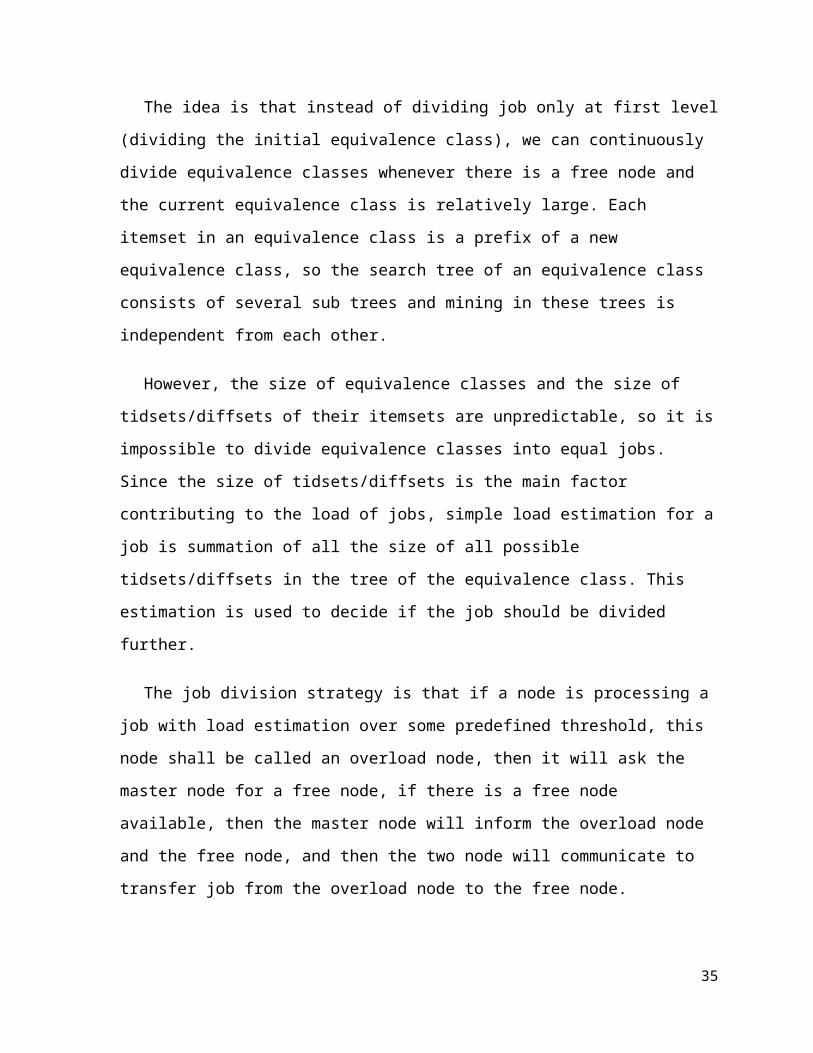
Figure 9 Initial database size at various values of minimum support in different formats

Eclat using combination tidset and diffset vs. dEclat

We compared com-Eclat and sorting-dEclat to show advantages of using combination

tidset and diffset. Because when minimum support is larger than 50 percent, the combination

format tends to adopt diffset format only, therefore we experimented only at minimum

support values lower than 50 percent. The figures below show the average set size and

running time of com-Eclat and sorting-dEclat at various values of minimum support on

databases.

Figure 10 Average set size of com-Eclat and sorting-dEclat at various values of minimum support

35

Figure 11 Running time of com-Eclat and sorting-dEclat at various values of minimum support

The general trend is that when minimum support increased, the gap between the average

set size of com-Eclat and sorting-dEclat tended to be widened while the gap between running

time of com-Eclat and sorting-dEclat tended to be narrowed. This is because with higher

minimum support values, the running times of both com-Eclat and sorting-dEclat were very

small and that made the gap smaller. That means that using the combination tidset and diffset

would be more beneficial if the minimum support is high (lower than 50 percent), especially

in terms of memory usage although it also made Eclat a little faster than dEclat.

In the cases of Mushroom and Pumsb_star, the average set size of sorting-dEclat was

much higher than that of com-Eclat. The reason here is that the conditional databases met the

switching condition but the number of their elements which did not satisfy the switching

condition was high, which led to a much higher average set size in comparison to that of

com-Eclat.

We noticed an interesting trend in the case of T40I10D100K where com-Eclat was

slower than sorting-dEclat, which may be because the cost of swapping diffsets and tidsets

outweighed the benefit of the reduction in set size. In the case of pumsb_star, when minimum

support was higher than 27 percent, the average set sizes of com-Eclat and sorting-dEclat

36

were almost the same because with minimum support higher than 27 percent com-Elcat

mainly used diffset.

2. Evaluate Performance of The Two Parallel Approaches

This thesis implemented the course-grained and fine-grained approach to evaluate the

performance gain in the proposed fine-grained approach. The parallel code is extended from

com-dEclat and implemented using MPICH2-1.3.2. We shall call the implementation of the

course-grained approach as course-dEclat and the implementation of the fine-grained

approach as fine-dEclat.

Experiments were run on a cluster of eight PCs; each is equipped with four Intel Q6600

2.4 GHz cores, 2 GB RAM and Linux 2.6.18 i686; PCs are connected by a Gigabit gateway.

Each experiment was run with four, eight, twelve, sixteen and twenty nodes to measure the

scalability of course-dEclat and fine-dEclat.

The figure below shows the load unbalancing problem of the coarse-grained approach.

The general trend is that the difference in running time of the earliest finished node and latest

finished node increases as the number of nodes increases. The difference in case of Pumsb*

is largest. And in this case, the overall performance did not improve as the number of nodes

increased. While in the case of T10I4D100K, the difference was very small and load

unbalancing seems not a problem for this dataset. In the case of Retail and T40I10D100K,

when the number of nodes was small, the difference was also very small but as the number of

nodes increased, the difference became more obvious.

37

Figure 12 Load Unbalancing Problem in Coarse-Grained Approach

The figure below shows the running time of coarse-dEclat and fine-dEclat on different

datasets. It could be seen that when the load unbalancing problem was serious, fine-dEclat

was faster that coarse-dEclat and when the load unbalancing problem was not serious, fine-

dEclat was slower than coarse-dEclat. The reason for this is that fine-dEclat has to check for

the job division condition and contact master node for free nodes. When the load unbalancing

was not a problem in coarse-dEclat, fine-dEclat could not improve its performance and it was

slower. However, this overhead cost in fine-dEclat was not significant and it was reduced as

the number of nodes increased, this is shown in the case of T40I10D100K and T10I4D100K.

In the case of Retail, when there were four or eight nodes, the load unbalancing problem was

not serious and fine-dEclat was slower than coarse-dEclat. However, as the number of nodes

increased, the load unbalancing problem got worse and at the same time fine-dEclat was also

gradually faster than coarse-dEclat.

38

Figure 13 Running time of coarse-dEclat and fine-dEclat on different datasets

39

Chapter 5

Conclusion

In this thesis we studied quite thoroughly dEclat algorithm and introduced a novel data

format for it, combination tidset and diffset, which uses both tidset and diffset formats to

represent a database in vertical layout. This new format can fully take advantages of both

tidset and diffset formats and eliminates the need for switching from tidset to diffset.

Experiments showed that it reduced memory usage of Eclat. It also speeded up Eclat though

not significantly. We showed the benefit of sorting diffsets in descending order and tidsets in

ascending order according to size, which significantly reduced the memory usage and

increased dEclat by several orders of magnitude.

We also proposed a new parallel approach for dEclat algorithm. This new approach could

address the problem of load unbalancing in the existing approach. Consequently, dEclat

using this new parallel approach could exploit the power of clusters or distributed systems

with many nodes. Experiments show that dEclat using our proposed parallel approach was

not suffered from load unbalancing problem and the approach had also increased the

scalability of dEclat when running in a parallel environment. In the case when datasets did

not cause load unbalancing problem for dEclat using the existing parallel approach, dEclat

using our proposed approach was just a little slower than dEclat using the existing parallel

approach; while in the case when dEclat using the existing parallel approach suffered from

load unbalancing problem, dEclat using our proposed parallel approach was significantly

faster than dEclat using the existing parallel approach.

40

Bibliography

[1] R. Agrawal, T. Imielinski, and A.N. Swami, "Mining association rules between sets of items

in large databases," in ACM SIGMOD International Conference on Management of Data,

Washington, 1993.

[2] R. Agrawal, and R. Srikant, "Fast algorithms for mining association rules," in 20th

International Conference on Very Large Data Bases, Washington, 1994.

[3] J. Han, J. Pei, and Y. Yin, "Mining frequent patterns without candidate generation," in ACM

SIGMOD International Conference on Management of Data, Texas, 2000.

[4] M.J. Zaki, S. Parthasarathy, M. Ogihara, and W. Li, "New algorithms for fast discovery of

association rules," in Third International Conference on Knowledge Discovery and Data

Mining, 1997.

[5] a. K. G. M.J. Zaki, "Fast vertical mining using diffsets," in The nineth ACM SIGKDD

International Conference on Knowledge Discovery and Data Mining, 2003.

[6] Paul W. Purdom, Dirk Van Gucht, and Dennis P. Groth, "Average case performance of the

apriori algorithm," vol. 33, p. 1223–1260, 2004.

[7] S. Orlando, P. Palmerini, R. Perego, and F. Silvestri, "Adaptive and resource-aware mining

of frequent sets," in Proceedings of the 2002 IEEE International Conference on Data

Mining, 2002.

[8] P. Shenoy, J.R. Haritsa, S. Sudarshan, G. Bhalotia, M. Bawa, and D. Shah, "Turbo-

charging vertical mining of large databases," in ACM SIGMOD International Conference on

Management of Data, 2000.

[9] B. Goethals, "Survey on frequent pattern mining," 2002.

[10] Yan Zhang, Fan Zhang, Jason Bakos, "Frequent Itemset Mining on Large-Scale Shared

41

Memory Machines," 2011.

[11] Mohammed Javeed Zaki, Srinivasan Parthasarathy, and Wei Li, "A Localized Algorithm for

Parallel Association Mining," in 9th Annual ACM Symposium on Parallel Algorithms and

Architectures, 1997.

[12] "Frequent Itemset Mining Dataset Repository," [Online]. Available: http://fimi.ua.ac.be/data/.

42