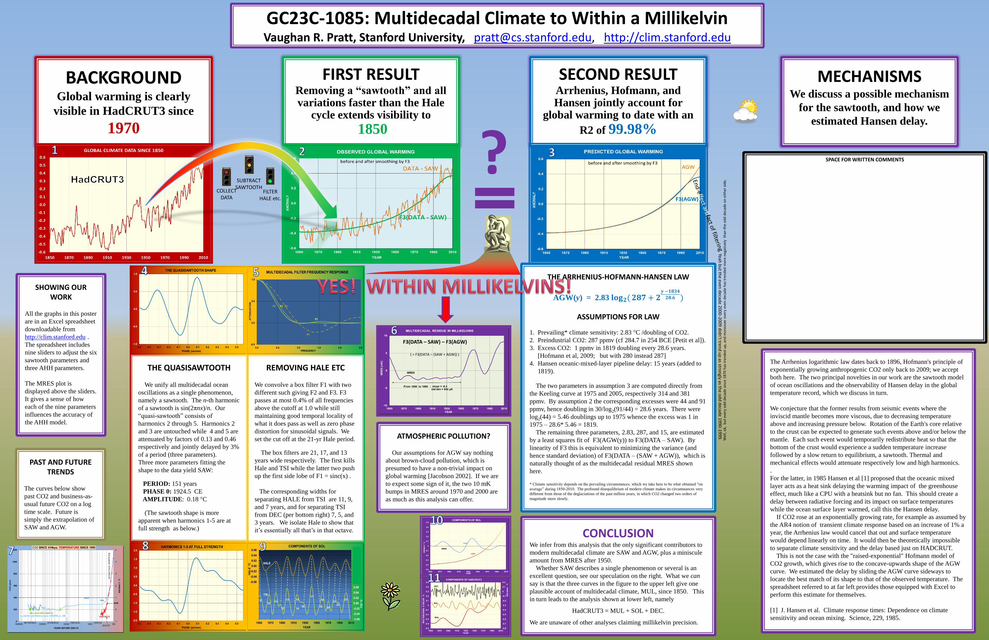
GC23C-1085: Multidecadal Climate to Within a Millikelvin Vaughan R. Pratt, Stanford University, pratt@cs.stanford.edu, http://clim.stanford.edu

FIRST RESULT Removing a “sawtooth” and all variations faster than the Hale

cycle extends visibility to

1850

REMOVING HALE ETC

We convolve a box filter F1 with two

different such giving F2 and F3. F3

passes at most 0.4% of all frequencies

above the cutoff at 1.0 while still

maintaining good temporal locality of

what it does pass as well as zero phase

distortion for sinusoidal signals. We

set the cut off at the 21-yr Hale period.

The box filters are 21, 17, and 13

years wide respectively. The first kills

Hale and TSI while the latter two push

up the first side lobe of F1 = sinc(x) .

The corresponding widths for

separating HALE from TSI are 11, 9,

and 7 years, and for separating TSI

from DEC (per bottom right) 7, 5, and

3 years. We isolate Hale to show that

it’s essentially all that’s in that octave.

ATMOSPHERIC POLLUTION?

Our assumptions for AGW say nothing

about brown-cloud pollution, which is

presumed to have a non-trivial impact on

global warming [Jacobson 2002]. If we are

to expect some sign of it, the two 10 mK

bumps in MRES around 1970 and 2000 are

as much as this analysis can offer.

CONCLUSION We infer from this analysis that the only significant contributors to

modern multidecadal climate are SAW and AGW, plus a miniscule

amount from MRES after 1950.

Whether SAW describes a single phenomenon or several is an

excellent question, see our speculation on the right. What we can

say is that the three curves in the figure to the upper left give one

plausible account of multidecadal climate, MUL, since 1850. This

in turn leads to the analysis shown at lower left, namely

HadCRUT3 = MUL + SOL + DEC.

We are unaware of other analyses claiming millikelvin precision.

PAST AND FUTURE TRENDS

The curves below show

past CO2 and business-as-

usual future CO2 on a log

time scale. Future is

simply the extrapolation of

SAW and AGW.

SECOND RESULT Arrhenius, Hofmann, and Hansen jointly account for

global warming to date with an

R2 of 99.98%

BACKGROUND Global warming is clearly

visible in HadCRUT3 since

1970

SHOWING OUR WORK

All the graphs in this poster

are in an Excel spreadsheet

downloadable from

http://clim.stanford.edu .

The spreadsheet includes

nine sliders to adjust the six

sawtooth parameters and

three AHH parameters.

The MRES plot is

displayed above the sliders.

It gives a sense of how

each of the nine parameters

influences the accuracy of

the AHH model.

MECHANISMS We discuss a possible mechanism

for the sawtooth, and how we

estimated Hansen delay.

The Arrhenius logarithmic law dates back to 1896, Hofmann's principle of

exponentially growing anthropogenic CO2 only back to 2009; we accept

both here. The two principal novelties in our work are the sawtooth model

of ocean oscillations and the observability of Hansen delay in the global

temperature record, which we discuss in turn.

We conjecture that the former results from seismic events where the

inviscid mantle becomes more viscous, due to decreasing temperature

above and increasing pressure below. Rotation of the Earth's core relative

to the crust can be expected to generate such events above and/or below the

mantle. Each such event would temporarily redistribute heat so that the

bottom of the crust would experience a sudden temperature increase

followed by a slow return to equilibrium, a sawtooth. Thermal and

mechanical effects would attenuate respectively low and high harmonics.

.

For the latter, in 1985 Hansen et al [1] proposed that the oceanic mixed

layer acts as a heat sink delaying the warming impact of the greenhouse

effect, much like a CPU with a heatsink but no fan. This should create a

delay between radiative forcing and its impact on surface temperatures

while the ocean surface layer warmed, call this the Hansen delay.

If CO2 rose at an exponentially growing rate, for example as assumed by

the AR4 notion of transient climate response based on an increase of 1% a

year, the Arrhenius law would cancel that out and surface temperature

would depend linearly on time. It would then be theoretically impossible

to separate climate sensitivity and the delay based just on HADCRUT.

This is not the case with the "raised-exponential" Hofmann model of

CO2 growth, which gives rise to the concave-upwards shape of the AGW

curve. We estimated the delay by sliding the AGW curve sideways to

locate the best match of its shape to that of the observed temperature. The

spreadsheet referred to at far left provides those equipped with Excel to

perform this estimate for themselves.

[1] J. Hansen et al. Climate response times: Dependence on climate

sensitivity and ocean mixing. Science, 229, 1985.

THE ARRHENIUS-HOFMANN-HANSEN LAW

AGW(y) = 2.83 𝐥𝐨𝐠𝟐( 𝟐𝟖𝟕 + 𝟐𝒚 −𝟏𝟖𝟑𝟒

𝟐𝟖.𝟔 )

ASSUMPTIONS FOR LAW

1. Prevailing* climate sensitivity: 2.83 °C /doubling of CO2.

2. Preindustrial CO2: 287 ppmv (cf 284.7 in 254 BCE [Petit et al]).

3. Excess CO2: 1 ppmv in 1819 doubling every 28.6 years.

[Hofmann et al, 2009; but with 280 instead 287]

4. Hansen oceanic-mixed-layer pipeline delay: 15 years (added to

1819).

The two parameters in assumption 3 are computed directly from

the Keeling curve at 1975 and 2005, respectively 314 and 381

ppmv. By assumption 2 the corresponding excesses were 44 and 91

ppmv, hence doubling in 30/log2(91/44) = 28.6 years. There were

log2(44) = 5.46 doublings up to 1975 whence the excess was 1 in

1975 – 28.6* 5.46 = 1819.

The remaining three parameters, 2.83, 287, and 15, are estimated

by a least squares fit of F3(AGW(y)) to F3(DATA – SAW). By

linearity of F3 this is equivalent to minimizing the variance (and

hence standard deviation) of F3(DATA – (SAW + AGW)), which is

naturally thought of as the multidecadal residual MRES shown

here. * Climate sensitivity depends on the prevailing circumstances, which we take here to be what obtained “on

average” during 1850-2010. The profound disequilibrium of modern climate makes its circumstances very

different from those of the deglaciations of the past million years, in which CO2 changed two orders of

magnitude more slowly.

SPACE FOR WRITTEN COMMENTS

?

Yeah b

ut th

e even d

ecade 2

00

0-2

00

9 d

idn

’t trend

up

as stron

gly as the o

dd

decad

e 19

90

-19

99

. Wel

l, o

k, b

ut

ever

y o

dd

dec

ade

sin

ce 1

87

0 h

as t

ren

ded

up

, an

d m

ore

ove

r ev

ery

even

dec

ade

has

tre

nd

ed m

ore

neg

ativ

ely

th

an t

he

od

d d

ecad

e o

n e

ith

er s

ide.

THE QUASISAWTOOTH

We unify all multidecadal ocean

oscillations as a single phenomenon,

namely a sawtooth. The n-th harmonic

of a sawtooth is sin(2πnx)/n. Our

“quasi-sawtooth” consists of

harmonics 2 through 5. Harmonics 2

and 3 are untouched while 4 and 5 are

attenuated by factors of 0.13 and 0.46

respectively and jointly delayed by 3%

of a period (three parameters).

Three more parameters fitting the

shape to the data yield SAW:

PERIOD: 151 years

PHASE 0: 1924.5 CE

AMPLITUDE: 0.18 °C

(The sawtooth shape is more

apparent when harmonics 1-5 are at

full strength as below.)

SUBTRACT SAWTOOTH

FILTER HALE etc.

COLLECT DATA

F3(DATA – SAW) – F3(AGW) ( = F3(DATA – (SAW + AGW)) )