3

Back to the Future:

International Trade Costs and the Two Globalizations1

Michel Fouquin2 and Jules Hugot3

This version: July 1, 2016

Abstract

This article provides an assessment of the nineteenth century trade globalization based on

a systematic collection of bilateral trade statistics. Drawing on a new data set of more than 1.9

million bilateral trade observations for the 1827-2014 period, we show that international trade

costs fell more rapidly than intra-national trade costs from the 1840s until the eve of World War

I. This finding questions the role played by late nineteenth century improvements in

transportation and liberal trade policies in sparking this First Globalization. We use a theory-

grounded measure to assess bilateral relative trade costs. Those trade costs are then aggregated

to obtain world indices as well as indices along various trade routes, which show that the fall of

trade costs began in Europe before extending to the rest of the world. We further explore the

geographical heterogeneity of trade cost dynamics by estimating a border effect and a distance

effect. We find a dramatic rise in the distance effect for both the nineteenth century and the

post-World War II era. This result shows that both modern waves of globalization have been

primarily fueled by a regionalization of world trade.

Keywords: Globalization, Trade costs, Border effect, Distance effect

JEL Classification: F14, F15, N70 Word count: 13,500

1. Introduction

1 We are grateful to Thierry Mayer, Kevin H. O’Rourke, Lilia Aleksanyan, Mathieu Crozet, Guillaume Daudin,

Sébastien Jean, Christopher M. Meissner, Dennis Novy, Paul S. Sharp for helpful comments. We thank Béatrice Dedinger

and Guillaume Daudin for giving us access to the RICardo data set. This research was improved by the comments from the participants of the EHS conference in Oxford, EEA conference in Malaga, EHA meeting in Vancouver, FRESH meeting in Edinburgh, EGIT workshop in Berlin, EHES conference in London, EBES in Istanbul, CIE in Salamanca, EHA meeting in Columbus, AEA in Yerevan, and seminars at CEPII, UQAM, P.U. Javeriana, Tbilisi State University (ISET), Istanbul Technical University, LSE-Kazakh-British Technical University, University of Bonn, Sciences Po, Université Paris-Sud (RITM), LSE and the Colombian Banco de la República.

2 CEPII (michel.fouquin@cepii.fr) 3 Pontificia Universidad Javeriana (jules.hugot@gmail.com)

4

The existence of two distinct periods of international market integration in the modern era – the

First Globalization of the nineteenth century and the post-World War II Second Globalization – has

been extensively documented. However, the precise chronology of the First Globalization remains

unclear. Understanding this timing is a necessary prerequisite to a proper analysis of the causes

behind globalization. Some argue that the First Globalization is a late nineteenth century

phenomenon, emphasizing the role of transportation technologies such as the steamship (Harley,

1988, Pascali, 2014), communication technologies such as the telegraph (Steinwender, 2014), and

pro-trade policies such as the gold standard (Estevadeordal et al., 2003, LópezCórdova and

Meissner, 2003). Others argue that the First Globalization took off in the early nineteenth century,

emphasizing the end of various trade monopolies as a trigger (O’Rourke and Williamson, 2002) or

the role played by improvements in transportation already achieved in the late eighteenth century

(Jacks, 2005).

We adopt a systematic approach to collecting trade statistics in order to explore the chronology and

geographical pattern of both globalizations. Specifically, we compile a data set that gathers more

than 1.9 million bilateral trade observations for the 188 years from 1827 to 2014. We also provide

data on aggregate trade, aggregate and bilateral tariffs, GDP, exchange rates and various bilateral

variables commonly used in the gravity literature.

We show that the obstacles specific to international trade fell steadily from the 1840s until World

War I This result creates a new temporal perspective for the factors that are claimed to be the

leading causes of nineteenth century globalization. Disentangling these factors, however, remains

beyond the scope of this paper. The early onset of trade globalization is consistent with evidence

on freight costs4 and on the European movement of unilateral trade liberalization,5but also with

those studies demonstrating that the trade treaties of the 1860s were of limited impact.6 However,

this paper challenges the studies that argue that late nineteenth century technological

improvements were the key driver behind the First Globalization.7

We also explore the geographical dynamics of globalization by disentangling between a border

effect and a distance effect. We show that both waves of globalization have been associated with

4 Harley (1988) finds that before the 1840s, freight rates fluctuated depending on the recurring wars that affected

Europe. He documents a continuous reduction of freight rates from c. 1840 to 1913. 5 The British repeal of the Corn laws is well documented (Sharp, 2010) but it was in fact a broader phenomenon.

Between 1827 and 1855, customs duties-to-imports ratios fell from 24% to 12% in France, from 33% to 15% in the U.K.

and from 3.5% to 2.3% in the Netherlands (Detailed sources in Fouquin and Hugot (2016)). 6 Accominotti and Flandreau (2006) and Lampe (2009) find that the Cobden-Chevalier network of treaties did not

contribute to expanding trade but merely substituted previous unilateral liberalizations. Lampe (2009), however, finds

some evidence of a trade-enhancing effect for particular commodities. 7 Pascali (2014) claims that "the adoption of the steamship [c. 1870] was the major reason for the first wave of trade

globalization" (p.23.).

5

an increasing response of trade to distance. In other words, both globalizations have been driven by

an increased regionalization of world trade patterns.

Trade globalization is the process by which international goods markets integrate. A simple

increase of world trade relative to output – the trade openness ratio – is therefore not sufficient to

diagnose globalization. In particular, trade openness is sensitive to the world distribution of

economic activity. Indeed, for a constant level of market integration, world trade openness increases

as the world economy becomes more scattered.8 In the long run, controlling for the dispersion of

the world economy is therefore necessary to properly grasp the evolution of trade globalization.

The economic history literature has adopted two distinct approaches to assess the extent of trade

globalization. The indirect approach looks at price-convergence. The direct approach relies on trade

statistics. The indirect approach builds on the intuition that, in the absence of international trade

costs, arbitrage should eliminate price gaps across countries. Empirically, this prediction has been

tested by measuring price gaps across different markets for the same commodity. This approach is

particularly helpful to investigate pre-modern globalization. 9 Indeed, the first comprehensive

customs reports were only drafted in the early eighteenth century, and only for a handful of

countries.10

Using data on colonial commodities such as cloves and pepper, O’Rourke and Williamson (2002)

observe price convergence across continents in the early nineteenth century. These commodities,

however, exhibit a high value-to-weight ratio, which makes them particularly worth trading. More

generally, the conclusions of such studies are product-dependent. For instance, using the same

approach, O’Rourke and Williamson (1994) show that the transatlantic convergence of meat prices

did not occur before c. 1900. Another caveat is that price gaps only reveal information on trade

costs when bilateral trade actually occurs and trade with third countries is negligible (Coleman,

2007). Finally, the price gap literature has focused on long-distance trade, while our data reveals

that by 1840 more than 50% of European trade was conducted within Europe.9

Our results bring support to the more recent strand of the price gap literature that claims that the

conditions for the First Globalization were in fact already met in the late eighteenth century. Those

8 Helpman (1987) shows that a rise of trade relative to income can result from a more even distribution of world GDP.

One simple illustration emerges from the comparison of two hypothetical situations. Imagine that consumers allocate

their expenditure to countries, including their own, in proportion to their GDP, i.e. that markets are perfectly integrated.

In the first situation, the world GDP is shared between two identical countries: world openness is therefore 50%. In the

second situation, there are 5 identical countries. Consumers therefore allocate 4/5 of their expenditure to foreign

countries. World trade openness is therefore 80%. 9 Sources of pre-modern price data include the records of the Dutch East India Company (Bulbeck et al., 1998), the

accounts of hospitals (Hamilton, 1934) and even Babylonian tablets (Földvári and van Leeuwen, 2000). 10 We collected trade statistics from 1697, 1703 and 1720, respectively for the thirteen colonies, Britain and France. 9This figure relies on a sample of five European countries: Belgium, France, the Netherlands, Spain and the U.K.

6

conditions could not translate into a surge of trade due to the recurring disruptive shocks that

plagued international relations until 1815. O’Rourke (2006) shows that international price gaps

widened during the Napoleonic Wars. He takes this as a sign that world markets were already well

connected in the late eighteenth century. Moreover, several authors find direct evidence of price

convergence in the eighteenth century. 11 The causes behind this nascent market integration,

however, remain unclear.12 What is certain is that the Congress of Vienna, in 1815, marked the

beginning of a century-long period of peace in Europe,12 associated with a rise of trade of an

unprecedented magnitude.

The direct approach to assessing the timing of globalization relies on observed bilateral trade. The

vast majority of these studies, however, focus on the 1870-1913 period13 (Estevadeordal et al., 2003,

Jacks et al., 2008, López-Córdova and Meissner, 2003). This may give the false impression that the

First Globalization began later than it actually did. Jacks et al. (2008) use trade statistics to infer

aggregate international relative trade costs. Their measure of trade costs builds upon the Head and

Ries index (2001), which is itself derived from the gravity equation. They find substantial trade cost

reductions between 1870 and 1913. Beyond the limitation in terms of temporal coverage, their

study concentrates on three countries: France, Britain, and the USA. As opposed to previous studies,

our work relies on a systematic collection of trade statistics before 1870 and back to 1827.14

We use aggregate international relative trade costs as a tool for evaluating the timing of

globalization. These trade costs are consistent with our definition of globalization as they are an

inverse measure of changes in trade that controls for the world distribution of production and

expenditure. While we rely on an aggregate measure, some authors have tried to measure individual

components of trade costs.15 This bottom-up approach has several drawbacks when it comes to

tracking overall trade costs over time. Indeed, trade costs range from observable barriers – such as

tariffs or freight costs – to a variety of unobservable features, such as language barriers and taste

preferences. Using the gravity model, Anderson and van Wincoop (2004) estimate that observable

trade barriers only account for a 20% tariff equivalent cost, out of a 74% typical international trade

11 Sharp and Weisdorf (2013) and Dobado-González et al. (2012) focus on British-American wheat trade, Rönnbäck

(2009) uses data on eleven colonial commodities, Jacks (2004) focuses on trade in the North and Baltic Seas. 12 One exception is Solar (2013), who documents a steep reduction of shipping costs between c. 1770 and c. 1820. 12The

Crimean War and the wars related to the German and Italian unification are the only exceptions. 13 Lampe (2009) is an exception as he collected product-level bilateral trade data for seven countries from 1857 to 1875.

His focus, however, is not on the timing of globalization, but on the heterogeneous effect of the CobdenChevalier

network of trade treaties across commodities. 14 Jacks et al. (2011) extend the sample to 130 country pairs, of which 61 do not involve France, Britain or the USA. By

comparison, our sample covers more than 42,000 country pairs, including about 1,500 country pairs for the 1827-1870

period. We provide a comparison of our data set with three others in Table 2. 15 Anderson and van Wincoop (2004) provide a survey of this literature.

7

costs for rich countries.16 Head and Mayer (2013) refer to these unobservable components as "dark

trade costs". They find that these hidden costs account for 72 to 96% of distance-related trade costs.

These results cast a long shadow on the possibility of recovering aggregate trade costs based on a

bottom-up approach.

We choose a top-down approach and use observed trade to infer aggregate international relative

trade costs. This method has the advantage of capturing all the possible components of trade costs

without having to assume an ad-hoc specification for each of them. On the flip side, the top-down

approach prevents us from identifying the individual components of trade costs.

The measure of trade costs we use takes its roots in the gravity literature. Specifically, we use the

Head and Ries index to relate observed trade to the frictionless counterfactual that emerges from

the structural gravity theory. Aggregate trade costs are inferred from this comparison. Economists

have derived gravity equations from a variety of general equilibrium trade models (Anderson and

van Wincoop, 2003, Krugman, 1980, Eaton and Kortum, 2002, Chaney, 2008, Melitz and Ottaviano,

2008). Head and Mayer (2014) review these micro-foundations and coin "structural gravity" the

models that involve multilateral resistance terms.17 These multilateral factors reflect the fact that

bilateral trade does not only depend on bilateral factors but also on the costs associated with the

outside option of trading with third countries. Head and Mayer (2014) show that all structural

gravity models yield the same macro-level gravity equation.

The generality of the gravity equation allows the skeptical reader to remain agnostic as to which

model best describes the fundamental reasons to trade. This becomes crucial when dealing with a

period of almost two centuries as it can be argued that the reasons to trade have changed

dramatically. 18 Beyond its generality, the Head and Ries trade cost index presents several

advantages. First, it perfectly controls for the country-specific determinants of trade emphasized by

the structural gravity literature, including supply and demand but also multilateral resistance terms.

Second, the Head and Ries index is bilateral-specific, which allows us to explore the dynamics of

globalization across trade routes. Third, the Head and Ries index can be converted into a tariff

16 We define observable trade barriers as freight costs plus protectionist policies. Anderson and van Wincoop (2004)

find that they respectively result in an 11% and a 8% tariff equivalent cost: 1.11 × 1.08 = 1.20. 17 Equation (2), p.8. Arkolakis et al. (2012) also emphasize the generality of the gravity equation. Similarly, Allen et al.

(2014) provide a unifying theory they call "universal gravity". 18 e.g. economies of scale have been claimed to become key drivers of trade after World War II (Krugman, 1980). 19We

have no reason to believe that the trade elasticity is volatile in the short run: Broda and Weinstein (2006) estimate the

elasticity of substitution for two recent periods: 1972-1988 and 1990-2001, at the product level. They find a small and

insignificant reduction in the median elasticity: from 2.5 to 2.2 (Table IV, p.568).

8

equivalent measure (Jacks et al., 2008), on the condition of imposing a value for the elasticity of

trade with respect to trade costs (hereafter: trade elasticity).

We also contribute to the literature by providing the first estimates of the trade elasticity for the

nineteenth century. The trade elasticity reflects the response of trade to trade costs in any structural

gravity model. A small trade elasticity reveals large incentives to trade, as agents are ready to pay

high costs to trade across borders. In the end, the larger the theoretical gains from trade, the higher

will be the measure of trade costs inferred from any given observed trade flows. The reasons why

the trade elasticity may have changed depend on the micro-level factors that push countries to

trade.19 In a monopolistic competition framework, product varieties may become closer substitutes

as more countries industrialize. In a Ricardian framework, productivity across sectors may become

more homogeneous due to technology convergence. Both these claims imply a reduction of the

theoretical gains from trade. As the potential gains peter out, consumers become more reluctant to

pay higher costs to obtain foreign goods. Trade therefore becomes more sensitive to trade costs

and the trade elasticity increases.

We use bilateral tariffs to identify the trade elasticity in both the cross section and the time

dimension. None of our estimates is statistically different from an interval between −5.24 and −5.39,

which is surprisingly close to the median value of −5.03 found by Head and Mayer (2014) in their

meta-analysis of trade elasticities estimated on World War II data. We conclude that the trade

elasticity did not substantially change over the last two centuries 19 and therefore use −5.03 as our

benchmark value.

We elicit differences in the dynamics of trade costs across trade routes. In particular, we show

that trade costs fell faster within Europe that across long distance routes during the nineteenth

century. We then make further use of the gravity equation to investigate the geographical pattern

of trade cost dynamics. Specifically, we decompose overall trade costs into a component that is

independent of the distance between the trading partners – the border effect – and a distance

effect. The border effect is the average trade reducing effect of international borders, once distance

is taken into account. The distance effect reflects the negative impact of distance on trade. This

decomposition, however, requires imposing an ad-hoc – although standard – functional form for

trade costs. In the end, we show that both waves of globalization have been disproportionately

fueled by an increase in short-haul trade. This feature has been documented for the Second

Globalization by Combes et al. (2008) and Disdier and Head (2008), but this article is the first to find

a similar pattern for the nineteenth century.

19 A stable aggregate trade elasticity could very well hide substantial changes at the commodity level.

9

As a last step, we provide a distance equivalent measure of the border effect, which shows that both

waves of globalization have been associated with borders becoming "thinner", i.e. that distance-

induced trade costs rose relative to border-related costs. This provides another way to illustrate the

increased regionalization of trade patterns over the course of both globalizations.

Section 2 discusses the Head and Ries index of trade costs. Section 3 introduces the data. In

Section 4, we estimate the trade elasticity for the nineteenth century. In Section 5, we estimate our

index of world trade costs. Section 6 explores the heterogeneity of trade cost dynamics across trade

routes. In Section 7, we decompose trade costs into a border and a distance effect, and compute a

measure of border thickness. Section 8 provides concluding remarks.

2. The Head and Ries measure of trade costs

The empirical literature has isolated particular components of international trade costs, such as

language barriers or transportation costs. This approach often comes at the cost of imposing

somewhat arbitrary functional forms for these barriers. Moreover omitted variable bias becomes a

source of concern as only a subset of the potential barriers are included in these regressions. Head

and Ries (2001) tackle this issue and derive a comprehensive index that infers trade costs from

observed trade flows. The Head and Ries index therefore captures both the observable and the

unnobservable components of trade costs.20 This feature is particularly appealing since data on the

components of trade costs is hardly available for the nineteenth century.

The Head and Ries index controls perfectly for the country-specific determinants of trade, including

supply and demand as well as multilateral resistance terms. In turn, the Head and Ries index

precisely reveals international trade costs relative to domestic ones, for each pair of country. On the

other hand, atheoretical measures, such as the trade openness ratio, do not allow to disentangle

between trade costs and internal factors.21 An example is given by Eaton et al. (2011) who document

a steep reduction of trade openness during the trade collapse of 2008-2009 while trade costs

remained rather stable.

Head and Ries derive their trade cost index from both the monopolistic competition model of

Krugman (1980) and a perfect competition model of national product differentiation, similar to

Anderson and van Wincoop (2003) (hereafter: AvW). The Head and Ries index relates observed

trade to the frictionless prediction that emerges from both models. The comparison of actual trade

to the frictionless counterfactual yields a measure of the aggregate trade barriers associated with

20 The Head and Ries index not only captures trade costs per se, but also home and third country-biased preferences

(e.g. if French consumers particularly dislike British products, the Franco-British trade cost will be high). The trade cost

measure that we eventually compute converts these preferences into a tariff equivalent. 21 Figure A.1 reports aggregate export openness ratios for six balanced samples.

10

each country pair. Novy (2013) shows that the Head and Ries index can be derived from a broader

range of models, including the Ricardian (Eaton and Kortum, 2002) and heterogeneous firms models

(Chaney, 2008, Melitz and Ottaviano, 2008).22 More generally, the Head and Ries index can be

derived from any structural gravity equation of the form:

Yi Xj

Xij = τij, (1)

Pi Πj

τ X` P τ`j Y` . ` indexes third countries.

where Pi` and Πj = ` P`

Bilateral trade (Xij) is positively related to production in the origin country (Yi), expenditure in the

destination country (Xj); and negatively related to the exporter’s outward multilateral resistance

term (Pi), the importer’s inward multilateral resistance term (Πj) and bilateral trade costs (τij). The

trade elasticity ( < 0) gives the response of trade to trade costs.

The multilateral resistance terms capture the fact that bilateral trade does not only depend on

bilateral factors but also on trade costs with third source and outlet countries.23 These terms provide

a challenge as they cannot be solved for analytically. Head and Ries (2001) provide an elegant

solution to cancel them out; as a result, they are able to obtain a ratio of bilateral relative to internal

trade costs. Multiplying equation (1) by its counterpart for the symmetric flow and assuming

balanced trade at the country level (Yi = Xi) yields:25

22 The AvW model builds upon an Armington demand structure to yield a gravity equation: trade occurs because of

consumers’ taste for variety. In the Ricardian model, trade occurs because of countries’ comparative advantages in

production. In heterogeneous firms models, trade is related to firms’ advantages in productivity. 23 In atheoretical estimations of the gravity equation, multilateral resistance terms were often approximated by a

weighted average of distance to third countries. See a discussion in AvW (2003), pp.173-174. Baldwin and Taglioni (2006)

refer to the omission of multilateral resistance terms as the "gold medal mistake" of the gravity literature. 25Novy (2007)

shows that the trade cost measure remains valid under imbalanced trade (Appendix A.3., p.32).

The gravity equation for internal trade writes:

11

Xij Xji = (Yi Yj) . (2)

Xij Xji = Xii Xjj. (5)

Rearranging and taking the geometric average of both directional relative trade costs yields the

Head and Ries index of trade cost:

. (6)

The Head and Ries index is a top-down measure: it makes use of theory to infer trade costs from the

observable variables in the right hand side of the equation. The Head and Ries index is also a relative

measure of trade costs: it evaluates the barriers to trading with a foreign partner, relative to internal

trade barriers. Any variation of the index can therefore reveal changes in international or intra-

national trade costs. The intuition is that the more countries trade internally24 as opposed to with

foreign partners, the larger international trade barriers must be relative to internal barriers. Trade

costs should a priori not be assumed to be symmetric. In this setting, however, only the geometric

average of both directional trade costs can be identified, which renders impossible to properly relate

trade costs to direction-specific explanatory factors.

Jacks et al. (2008) propose a tariff equivalent interpretation of the Head and Ries index. In the

general framework of structural gravity, their measure of trade costs writes:

24 We discuss the measure of internal trade we use in Section 3.

Yi2

Xii = τii.

Pi Πi

Rearranging equation (3) yields an expression for Pi Πi (Pj Πj):

(3)

Yi2 τii

Pi Πi = .

Xii

Plugging the previous equation for Pi Πi and Pj Πj back into equation (2) yields:

(4)

s

12

1

Xii Xjj

TCij − 1.

(7)

Xij Xji

To illustrate equation (7), let us consider two perfectly integrated markets. For this pair of countries,

the international trade barriers are nil. The tariff-equivalent trade cost must therefore equal zero.

In turn, the ratio in the right hand side of equation (7) must be equal to one. In other words, in a

frictionless world, the product of two countries’ internal trade should be equal to the product of the

bilateral flows that link them.

Computing the Jacks et al. (2008) measure of trade costs requires to set a value for the trade

elasticity. In the benchmark results, we set to -5.03, which is the preferred estimate from the meta-

analysis of Head and Mayer (2014).25 In Section 4, we provide our own estimates for the nineteenth

century and show that they are not significantly different from our benchmark value.

3. Data

One distinctive feature of this research has been to systematically collect bilateral and aggregate

trade data as well as GDP and exchange rates between 1827 and 2014. Fouquin and Hugot (2016)

provide a detailed description of the data. Here we simply emphasize some key features.

Table 1 provides a summary of the main variables. Table 2 compares our data with three bilateral

trade data sets of reference. In order for these comparisons to be meaningful, we compare each of

these data sets with the sub-sample of our own data that covers the same period.26 At constant time

coverage and in terms of the number of observed trade flows, our data set is therefore more than

twice as large as (Pascali, 2014), about 11 times larger than (Jacks et al., 2011) and more than 6

times the size of (Barbieri and Keshk, 2012).

Bilateral Total Total GDP Exchange Bilateral

trade exports imports rates tariffs

Dimension country-pair country country country country country-pair

25 Specifically, we use the median coefficient from their meta-analysis, restricted to the structural gravity estimates

identified through tariff variation (see Table 5, p.33). 26 We restrict the samples to the years before 1948 because all the data sets rely on the same data from the IMF after

that point.

13

direction-year1 year year year year direction-year

Number of observations 1,904,574 21,085 20,869 14,084 14,381 8,720

Number of country pairs 42,447 410

Number of countries2 319 247 245 218 145 172

1 Each year, in theory, two trade flows pertain to each country pair: the exports from country A to country B and the exports from country

B to country A. 2 We use the word "country" to designate any administrative entity for which bilateral data is reported.

Table 1 – Summary of the main variables

Coverage Our data Pascali Jacks et al. Barbieri and

(2014) (2011)1 Keshk (2012)

Bilateral trade flows

51,710 23,0002

Country pairs 1850-1900 2,476 1,0002

Countries 191 129

Bilateral trade flows

238,850

21,806 38,646

Country pairs 1870-1947 14,497 298 2,036

Countries 295 27 68

1 We use the data from which the balanced sample used in Jacks et al. (2011) has been extracted. 2 Approximated figures extracted from Pascali (2014), p.2.

Table 2 – Comparison of the bilateral trade data with three data sets of reference, at constant time

coverage

The use of bilateral trade data to compute international relative trade costs is straightforward, but

the results also depend on the measure of internal trade. Unfortunately, data on aggregate

domestic shipments does not exist for as large a spatial and time coverage. Instead, we use a

measure of gross output, from which we subtract aggregate exports. Most gravity-oriented articles

on nineteenth century trade use constant price GDP data from Maddison (2001) (Jacks et al., 2008,

2011, Pascali, 2014, Estevadeordal et al., 2003, López-Córdova and Meissner, 2003) sometimes

14

reflated using the U.S. price index.27 On the other hand, the structural gravity theory demands that

both trade flows and GDP are entered in nominal terms. Indeed, the gravity equation is a function

that allocates nominal expenditures across countries, i.e. that allocates nominal GDP into nominal

imports. We therefore rely exclusively on nominal series.

Internal trade, as any measure of trade, is a gross concept in the sense that it includes intermediate

goods. It should thus be measured as gross domestic tradable output, minus total

exports.28Unfortunately, reconstructions of national accounts have concentrated on GDP series that

are by definition net of intermediary consumption. Our approach is to use the average ratio of gross

output to value added taken from de Sousa et al. (2012) to scale up current price GDP data and

obtain an approximation of gross output.31 We finally subtract total exports and use the resulting

series as our benchmark measure of internal trade.29

4. Estimation of the trade elasticity

The trade elasticity is a necessary parameter to infer trade costs from trade data. Indeed, a strong

response of trade to trade costs translates in lower trade costs being inferred from the same data.

In the extreme case, if consumers are infinitely sensitive to trade costs, then the absence of trade

does not reveal prohibitive trade costs, but simply a total lack of interest for foreign goods. In our

case, any observed reduction of trade costs can therefore be genuine, or an artifact due to a fall in

the (absolute) trade elasticity over time. Checking for long run trends in the trade elasticity is

therefore crucial to establishing the robustness of our results. Beyond our direct interest, the trade

elasticity is also a key parameter in the recent literature which aims at recovering the welfare gains

from trade. In particular, Arkolakis et al. (2012) show that in a broad class of trade models two

statistics are sufficient to calculate countries’ welfare gains from trade: the import openness ratio

and the trade elasticity. Historical estimations of the trade elasticity are therefore a necessary

27 Baldwin and Taglioni (2006) coined this adjustment of GDP series the "bronze medal mistake" in the gravity literature:

"Since there are global trends in inflation rates, inclusion of [the U.S. price index] probably creates biases via spurious

correlations", p.7. 28 Gross output = GDP + Intermediary consumption. Measuring internal trade as Gross output − exports is especially

relevant for countries that are very open to trade, as for some years, failing to adjust GDP for intermediate consumption

would result in negative internal trade. For further discussion, see Head and Mayer (2014), p.169. 31Specifically, we

aggregate their figures across industrial sectors to obtain an average ratio of 3.16. We then take the product of this ratio

and GDP as a measure of gross output. 29 We provide alternative results with internal trade measured as: Tradable GDP − exports. To do so, we decompose

GDP into a tradable (agriculture and industry) and a non-tradable component (services). We scale-up this data using

ratios of value added to gross production. For the industrial sector, we use the ratio from de Sousa et al. (2012). For

agriculture, we use a ratio of 2.4 (INSEE, Compte provisoire de l’agriculture, May 2013). This comes at the cost of

restricting the sample to 58% of its full potential. In Figure A.15, we estimate our world trade cost index using this

alternative method.

15

prerequisite to any structural investigation of the welfare gains associated with nineteenth century

trade.

Head and Mayer (2014) show that in any trade model that yields structural gravity, the trade

elasticity is related to the parameter that governs the scope for trade gains. More precisely, the

response of trade to trade costs decreases with the potential trade gains. It is thus necessary to look

into the models to understand the micro-level reasons for changes in the trade elasticity.

In the demand-side models of AvW (2003) (perfect competition) and Krugman (1980) (monopolistic

competition), the trade elasticity is linked to the elasticity of substitution across varieties ( = 1 − σ).

Countries trade to satisfy consumers’ love of variety. In turn, when varieties are close substitutes

(large σ), the incentives for trading narrow and the (absolute) trade elasticity increases. An

increasing similarity of the goods produced across countries would therefore lead to a rise of the

trade elasticity. In supply-side models such as the Ricardian model (Eaton and Kortum, 2002) and

heterogeneous firms models (Chaney, 2008, Melitz and Ottaviano, 2008), θ (γ) is the parameter that

governs the degree of heterogeneity of industries’ (Ricardo) or firms’ productivity (heterogeneous

firms). The less heterogeneity on the production side (large θ or γ), the smaller the scope for trade

gains and the larger the trade elasticity. An homogenization of industries’ or firms’ productivity

would therefore lead to a rise of the trade elasticity.

We follow Romalis (2007) and use bilateral tariffs to identify the trade elasticity in both the cross

section and the time dimension using French data for 1829-1913. The identifying assumption is that

tariffs are pure cost shifters, i.e. that trade costs react one for one to changes in tariffs. We begin

with the structural gravity equation:

τijt = (1 + tijt) × Distijα1 × exp(α2 Coloijt) × exp(α3 Comlangij)

(9) × exp(α4 Contiij) × ηijt,

where tijt is a measure of bilateral tariffs. Distij is the population-weighted great-circle distance.

Coloijt, Comlangij and Contiij are three dummies that account for colonial relationship, common

language and a shared border. ηijt reflects the unobserved components of trade costs.

We estimate the trade elasticity using the ratio of bilateral customs duties to imports as a proxy for

bilateral tariffs. A caveat should be noted: tariffs have an ambiguous link to these ratios. First, higher

tariffs increase the value of the customs duties that are collected. At the same time, tariffs reduce

Yit Xjt

Xijt = τijt.

Pit Πjt

We specify trade costs as follows:

(8)

16

imports by making imported goods more expensive30. The resulting duties-to-imports ratios may

therefore underestimate the actual level of protection. In turn, the trade elasticities we estimate

should be considered as lower bounds (in absolute terms).

We obtain the cross-section equation by plugging equation (9) into (8), taking logs and removing

time subscripts. We estimate the resulting equation separately for each year using OLS. The notation

explicitly specifies that France is always the destination country:

ln XiFR = ln(1 + tiFR) + γ ln Yi + β1 ln DistiFR + β2 ColoiFR (10) + β3 ComlangiFR + β4 ContiiFR + ln ηiFR.

We use the notation βx = αx ×, ∀ x ∈{1, 2, 3, 4}. Yi is the GDP of country i. The error term (ηiFR) captures

the bilateral components of trade costs that are not explicitly controlled for, as well as origin

countries’ outward multilateral resistance terms. As a result, the trade elasticities obtained from

equation (10) cannot be considered as structural estimates.31

We also identify the trade elasticity in the time dimension, using decade-long intervals. This time,

we keep the time subscripts and impose a set of origin-country fixed effects. The identification

therefore entirely comes from the time dimension:

ln XiFRt = ln(1 + tiFRt) + FEiFR + γ1 ln Yit + γ2 ln YFRt

(11) + β2 ColoiFRt + ln ηiFRt.

The error term (ηiFRt) captures the time-varying unobserved components of trade costs, as well as

the time-varying components of both inward and outward multilateral resistance terms. The

coefficients estimated using equation (11) thus do not qualify as structural gravity estimates.

Figure 1 shows that the estimated trade elasticities are never different from each other at the 95%

confidence level, which suggests that the trade elasticity has not changed significantly over the

nineteenth century. We find a median elasticity of -4.84 [2.40] and −5.07 [.70], respectively in the

cross section and the time dimension. None of these estimates is statistically different at the 95%

level of confidence from −5.03, the median value found in the meta-study of Head and Mayer

30 In particular, the prohibitive tariffs that were imposed on some products until the late nineteenth century result in an

underestimation of the actual level of protection. See the Irwin-Nye controversy (Nye, 1991, Irwin, 1993). 31 Obtaining structural estimates would require controlling for both origin and destination country multilateral

resistance terms, for example through two sets of fixed effects. This would require bilateral tariff data for more than

one country, which we were unfortunately unable to find.

17

(2014). We take this as a sign that the trade elasticity did not substantially change between the early

nineteenth and the late twentieth century.32 The results of the following sections rely on a constant

trade elasticity of −5.03.

Cross-section estimation Time series estimation (by decade)

The shaded areas represent 95% confidence intervals

Figure 1 – Cross-sectional and longitudinal estimations of the trade elasticity: 1829-1913

5. World trade cost indices

Once equipped with a value for the trade elasticity, we can use equation (7) to compute trade costs.

We obtain more than 370,000 measures of trade costs for about 14,000 country pairs. Reporting all

of the results would be impossible; instead, we report selected aggregates.

We begin by restricting the sample to the country pairs for which we obtain trade costs on a

continuous basis throughout the period. 33 Figure 2 reports weighted-mean trade costs for four

balanced samples (Figure A.2 reports the simple mean).37 Specifically, we weight trade costs by the

32 However the standard errors are too large to claim that nineteenth century trade elasticities lied closer to the lower

or the upper bound of the post World War II estimates, which typically range from −1 to −7. 33 In order to increase the number of country pairs included in the samples, we interpolate missing trade costs if the

following criteria are all satisfied: i) trade costs are observed for the initial and the last year of the sample, ii) observed

trade costs account for at least 90% of potential observations, iii) gaps are inferior or equal to 5 years. 37The 1827 sample

covers: CHL-FRA, CHL-USA, DNK-FRA, ESP-FRA, ESP-GBR, ESP-PRT, ESP-USA, FRAGBR, FRA-PRT, FRA-USA, GBR-USA. The

1835 sample adds: BEL-DNK, BEL-ESP, BEL-FRA, BEL-GBR,

BEL-NLD, BEL-USA, COL-FRA, COL-USA, DNK-NLD, DNK-SWE, ESP-SWE, FRA-NLD, FRA-NOR, FRASWE, GBR-NLD, GBR-SWE, NLD-USA, NOR-SWE, SWE-USA, while ESP-PRT and FRA-PRT leave the sample.

18

sum of the two countries’ internal trade. We use the same aggregation method to compare

transatlantic and intra-European trade costs (Figure A.3).

Aggregating trade costs over all available country pairs is not trivial since the sample changes over

time (Figure 3). In particular, the composition of the sample may be endogenously determined as

most data for early years comes from the most developed countries. In turn, exchanges among

these countries are associated with structurally low trade costs. Ignoring this sampling bias would

thus result in an underestimation of any trade cost reduction. On the other hand, limiting the

analysis to balanced panels considerably reduces the information available. In particular, many

countries are simply formed or dismantled during our two centuries of interest, which

19

1840 1860 1880 1900 1920 1940 1960 1980 2000 1827 (11)

1835 (28) 1870 (93) 1921 (236)

The legend reports the initial year of each sample (# of pairs in each sample in parenthesis) The two world wars are omitted from the samples

Figure 2 – Internal trade-weighted mean trade

costs, balanced samples

20

Figure 3 – Number of computed bilateral trade

costs

34 We compute 14 bilateral trade costs for 1827 and

about 9,000 for 2014. Over time, the number of

computed trade costs tends to increase, to the

exception of the two world wars, which temporarily

reduce data availability. 39We estimate equation (12)

using the reghdfe command from Stata, which is itself

a generalization of the xtreg,fe command that allows

for unbalanced panels. 35 see footnote 36. 36 These sub-periods are: 1835-1870, 1871-1912,

1921-1937, 1950-1980 and 1981-2014.

automatically rules them out from any balanced sample.34 We therefore propose an index of trade

costs that makes use of all of the information available while also partially controlling for the

sampling bias. Specifically, we decompose trade costs into a bilateral and a time effect:39

ln TCijt = αij FEij + βt FEt + ηijt. (12)

The bilateral effects capture the factors that are both country-pair-specific and time-invariant (e.g.

distance, long-run cultural ties, etc.); but the pairs included in the sample vary over time. In turn,

exp(βt) is the expectation of trade costs in year t relative to the benchmark year, conditional on the

country pairs available in year t. Figure 4 plots exp(βt), which is our index of world trade costs. Figure

A.4 plots the former against a trade cost index that is obtained by weighting each observation by

the total value of both partner’s internal trade. Figure A.4 shows that the long-run trends of the

trade cost index are not driven by small countries.

Despite our correction, the trade cost index remains subject to a composition bias, as we estimate

the conditional expectation of the log of trade costs on a sample that varies over time. The only way

to eliminate this bias is to estimate equation (12) using balanced samples. Figure 5 shows the

resulting indices estimated on five samples.35 Figure 6 replicates the exercise but this time using five

sub-periods that do not extend until 2014.36 Finally, Figure 7 plots the

21

1840 1860 1880 1900 1920 1940 1960 1980 2000 The shaded area represents the 95% confidence interval

Figure 4 – World trade cost index

) The legend reports the initial year of each sample (# of pairs in each sample in parenthesis) The two wold wars are omitted from the samples

Figure 5 – World trade cost indices, balanced

samples

world trade cost index estimated on balanced two-year samples. The resulting estimates are then

chained to obtain a global picture of the evolution of trade costs.

Figures 4 to 7 both show a steady fall of trade costs that begins in the late 1840s and lasts until

World War I. Trade cost indices return to their 1913 levels soon after the war. Not surprisingly, the

Great Depression is associated with a rise of trade costs that extends into World War II. Trade costs

then quickly recover their pre-war level in the 1950s.37 Trade costs remain rather stable in the three

decades after World War II before resuming to fall in the late 1970s.

The level of trade costs is sensitive to the value of the trade elasticity. Figure A.5 reports the

Franco-British trade cost obtained using alternative trade elasticities. As a thought experiment,

Figure A.6 also imposes an increasing and a decreasing linear trend for the trade elasticity, using −3

and −7 as extreme values. A reduction of the (absolute) value of the trade elasticity reveals larger

scope for trade gains. In the end, any observed trade cost reduction could in fact be due to a

37 Figure 5 provides a somewhat different picture as

trade costs take more than 20 years to recover their

prewar level for the the most restricted samples. This

divergence is due to an over-representation in these

samples of the countries that suffered the most from

the war.

1827 (11) 1835 (28) 1870 (93) 1921 (236) 1960 (1449

22

reduction of the (absolute) trade elasticity. However, Section 4

has established the stability of the trade elasticity for our

period of interest.

6. Route-specific trade cost indices

We now explore the heterogeneity of trade costs across trade routes. Specifically, we estimate trade

cost indices based on various sub-samples. Figure 8 plots indices obtained by aggregating The legend reports the initial year of each sample (# of pairs in each sample in parenthesis)

Figure 6 – World trade cost indices, Figure 7 – World trade cost index, chained balanced

samples estimates from two-year balanced samples

bilateral trade costs across all partners for three countries. 38 For the nineteenth century, the

patterns for France and the U.K. are similar as the largest reduction of trade costs happens between

the early 1850s and the 1870. Trade costs then remain almost stable until the Great Depression. The

patterns diverge after World War II. While trade costs trend downwards for France until the 1980s,

they start rising after 1980 for the U.K.. This means that trade costs within the U.K. have been falling

faster than international trade costs for the recent period. The dynamics of trade costs affecting the

United States is very different as the steady fall of trade costs only begins around 1870. Trade costs

only recover to their antebellum low point around 1890, which illustrates the long-lasting effect of

the Civil War on U.S. foreign trade, through the protectionist policies imposed by the victorious

North. Figure A.7 reports additional trade cost indices for Belgium, the Netherlands, Spain and

Sweden.

38 Note that for country-specific aggregations, equation (12) writes: ln TCit = αi FEi +βtFEt +ηit, where i indexes the trading

partners of the country of interest. Figure A.8 reports the corresponding chained trade cost indices, estimated on

balanced two-year samples.

1835 (25) 1950 (820) 1871 (120) 1921 (288)

1981 (2544)

23

Figure 9 plots trade cost indices for three regions.39 Specifically, we aggregate trade costs across all

the country pairs that include a country of the region of interest. Figure 9 shows that trade costs

start falling for core European countries in the late 1840s. For the European periphery and the rest

of the world, the high volatility prior to 1880 is followed by a dramatic reduction of trade costs

around the turn of the century. All three regions are affected by comparable rises of trade costs

during the Great Depression and World War II. After the war, trade costs remain rather stable for

Core Europe, while they fall for the European periphery. Trade costs for the rest of the world are

stable until they resume falling in the early 1990s.

39 Core Europe corresponds to Northwestern Europe. The European periphery includes Central, Eastern and Southern

Europe, together with Scandinavia. See region coding in Fouquin and Hugot (2016). Figure A.9 reports the corresponding

chained trade cost indices, estimated on balanced two-year samples.

24

1840 1860 1880 1900 1920 1940 1960 1980 2000 To facilitate comprehension, the French and British trade cost index are not reported for 1941-1945 and 1942-1944 respectively

Figure 8 – Trade cost indices: France, U.K., USA

1840 1860 1880 1900 1920 1940 1960 1980 2000 To facilitate comprehension, the trade cost indices for Core Europe and the European Periphery are not reported for 1943-1944

Figure 9 – Trade cost indices: Core Europe, European Periphery, Rest of the

world

40 In 1868, the U.S. aggregate tariff reaches 45% (see

Figure A.10). Tariffs remain consistently high until

World War I, fluctuating between 20% and 30%, roughly

twice as high as in France and the U.K..

France United Kingdom USA Core Europe European Periphery Rest of the World

Figure 10 takes a closer look at the dynamics of trade costs across Europe. The patterns are relatively

similar during the nineteenth century, except that trade costs affecting Northwestern Europe fall

more steadily. After World War II, trade costs remain stable for Northwestern Europe and

Scandinavia, but they resume falling for Southern European countries.

Figure 11 shows that trade costs also follow different patterns across trade routes. Transatlantic

trade costs are very volatile until the reduction that occurs between 1890 and World War I. The U.S.

Civil War is accompanied by a spike of trade costs, followed by a quick recovery, despite the

persistent high level of tariffs imposed by Northern states.40 It therefore seems that the high level

of protection was more than compensated by improvements in transportation and communication

technologies (Pascali, 2014, Steinwender, 2014).

After the initial spike that affects intra-European trade (Scandinavia in particular), trade costs fall

faster within Europe than across the Atlantic. The most dramatic fall of trade costs across the

Atlantic occurs in the decade before World War I. Intra-European trade costs are also more affected

by the Great Depression and the two world wars. After World War II, intra-European trade costs fall

while transatlantic trade costs increase, which points to the success of the European integration and

the consecutive relative dis-integration of transatlantic trade.

25

1840 1860 1880 1900 1920 1940 1960 1980 20

00

Core Europe Scandinavia Southern Europe

To facilitate comprehension, the trade cost indices for Core Europe and Scandinavia are not reported for 1943-1944

Figure 10 – Trade cost indices: Northwestern Europe, Scandinavia,

Southern Europe

7. Regionalized globalizations

Intra-Europe Intra-America Transatlantic

To facilitate comprehension, the trade cost index for Transatlantic trade is not reported for 1941-1944

Figure 11 – Trade cost indices: intra-European

trade, intra-American trade, transatlantic trade

The previous section emphasizes the heterogeneity of trade costs dynamics across trade routes.

Here, we further explore the geographical dynamics of trade globalization. Once more, we begin

with the structural gravity equation:

Yi Xj

Xij = τij. (13)

Pi Πj

We impose the following functional form for bilateral trade costs:

τij = exp(a Forij) × Distijb × ηij, (14)

26

where Forij is a dummy variable set to unity if i 6= j. Distij|i6=j is the population-weighted great-circle

bilateral distance and Distij|i=j is internal distance.41 a and b are the elasticities of trade costs to

international borders and distance respectively. ηij reflects the unobserved components of trade

costs, including for example bilateral tariffs.

Plugging (14) into (13), taking logs and imposing origin and destination fixed effects to control for

the monadic determinants of trade, we estimate equation (15), separately for each year, using the

OLS estimator. The identification comes entirely from the cross-sectional variation:42

ln Xij = FEi + FEj + β1 Forij + β2 ln Distij + ln ηij, (15)

where Xij|i6=j is bilateral trade and Xij|i=j is internal trade. FEi and FEj are vectors of origin and

destination fixed effects. β1 = a × is the border effect and β2 = b × is the trade elasticity of distance.

Note that the fixed effects perfectly control for the monadic determinants of trade, including

multilateral resistance terms. Because the errors are likely correlated within country pairs, we

cluster the standard errors at the bilateral level.

7.1. Border effect

β1 can be interpreted as a border effect as it reflects the average trade reducing effect of

international borders, all monadic determinants of trade and distance being equal. We convert the

border effect into a tariff equivalent using the pure cost-shifter property of tariffs.43. Indeed, ad-

valorem tariffs have a one for one relationship to trade costs. In turn, the error term of equation

(15) can be decomposed as follows:

ηij = (1 + tij)1 × Zij, (16)

where tij is the (unobserved) ad-valorem tariff imposed by j on imports from i. Zij is a vector of the

other bilateral components of trade costs, together with their elasticities to trade costs.

41 For details on these variables, see Fouquin and Hugot (2016) 42 The identification of the border effect relies on a comparison of internal trade with bilateral trade as in Wei (1996),

who extended the methodology introduced by McCallum (1995) for cases in which bilateral intra-national trade flows

are not available. 43 Figure A.11 reports the border effect as the exponential of β1. These values read as the number of times countries

trade more, on average, with themselves than with foreign partners, all monadic terms and distance being equal.

27

The border effect we propose is equal to the tariff that would have the same trade reducing

effect as the average border. We therefore use the β1 estimated for each year via equation

(15) to solve for the border effect (BE) in the following equation:

(1 + BE) = exp(β1).

The resulting tariff-equivalent border effect, converted to a percentage, writes:

(17)

BE × 100. (18)

28

Figure 12 reports the border effect with the trade elasticity () set to our benchmark value of −5.03.44

Overall, the border effect falls from approximately 300% c. 1830 to about 150% for most recent

years. More precisely, the border effect falls until World War I, with two episodes of stagnation: in

the 1840s and the two decades between 1860 and 1880. Not surprisingly, the border effect rises

during the Great Depression and until after World War II, before resuming a steady fall from the late

1960s. In 2014, which is the last year of the sample, the border effect has still not reached its low

point of 1920.

Our estimates are higher than those typically found in the literature. The pioneering study by

McCallum (1995) found that the U.S.-Canada border reduced trade by a factor 22 in 1988. AvW

(2003) provided the first structural estimation of the border effect (i.e. controlling for the

multilateral resistance terms) and found that the U.S.-Canada border reduced trade by a factor 5.

For the corresponding years and based on our entire sample, we find a border effect about 15 times

larger than McCallum’s and 37 times larger than AvW’s. 45 These results can be reconciled by

acknowledging that both McCallum (1995) and AvW (2003) consider the border between two

advanced economies. On the contrary, our sample is much broader. In fact, reducing the sample to

developed countries dramatically reduces the discrepancy. For example, estimating the border

effect on E.U. internal trade yields estimates that are only 4.5 times as large as those of AvW (2003)46

(Figure 13). In contrast, our estimates are perfectly in line with the border effects estimated on

samples similar to ours for the recent period (de Sousa et al., 2012).52

The reduction of the border effect since the 1970s is a well-established result. Helliwell (1998) was

the first to document that phenomenon, for 1991-1996. Head and Mayer (2000) provide structural

estimates for the E.U., based on data for 1975-1995. Finally, de Sousa et al. (2012) extend the sample

to the entire world, for 1980-2006 and still reach the same conclusion. In contrast, we bring a new

perspective on border-related trade barriers for the century and a half before 1970. In particular,

Figure 12 shows that the border effect fell by about one third between 1850 and World War I. Then

they doubled between 1920 and 1955 before falling again. Consequently, the border effect is close

in 2014 to its level during the run-up to World War I. In order to find a border effect as high as in

1955, one has to go back in time to 1831. The border effect thus appears to have followed similar

trajectories during both period of globalization.

44 Both the level and the variability of the border effect are sensitive to the value of the trade elasticity. Figure A.16

reports tariff-equivalent border effects obtained using different trade elasticites. 45 For 1988, we find a border effect equal to -5.77, which implies that ceteris paribus, countries traded on average 314

times more within their borders than with foreign partners (exp(5.77 = 321)). For 1993, we find a coefficient of -5.22

(i.e. a factor of 185). 46 For E.U. member countries as of 1995, we find a coefficient equal to -3.11, which corresponds to a factor 22. 52They

find a border effect of -5.97 for the 1980-2006 period (p.1043), while we find -5.51.

29

7.2. Distance elasticity

Figure 14 illustrates the rise of the distance elasticity with an example. From 1850 to 1914 the GDP

of Chile grew three times faster than the Dutch GDP. Between World War I and 1840 1860 1880 1900 1920 1940 1960 1980 2000

The shaded area represents the 95% confidence interval Standard errors clustered at the bilateral level

Figure 12 – Tariff-equivalent border effect

All observations OECD (1964 members)

EU (1995 members)

Figure 13 – Tariff-equivalent border effect: Full

sample, OECD, E.U.

2014 the GDP of both countries rose by similar magnitudes.47 Following the logic behind the gravity

model, one would expect that trade between Chile and, say, the U.K. would have at least increased

as fast as between the Netherlands and the U.K.. Figure 14 shows that in fact, trade increased much

faster with the proximate country (the Netherlands) than with the distant country (Chile) during

both waves of globalization.48 Another way to grasp the intuition behind the changes in the distance

elasticity is to look at the distribution of trade by distance for a given country. Figure A.17 presents

evidence from the Netherlands. These graphs suggest that distance was an increasingly important

47 Between 1850 and 1913, the Dutch GDP grew by 300%, while the Chilean GDP grew by 900%. Between 1948 and

2014, the GDP of both Chile and the Netherlands grew by 11,000% (in nominal terms). 48 British exports to the Netherlands grew by 3.52% per year during the First Globalization and by 10.41% per year after

World War II. Over the same periods, British exports to Chile only grew by 1.97% and 7.87% per year. 55Disdier and Head

(2008) show in their meta-analysis that the rise of the distance effect cannot be explained by sampling error. They argue

that the actual distance elasticity rose from about -0.7 in 1960 to -1.1 in 2000. They coin this phenomenon the "distance

puzzle".

30

factor in determining trade patterns during the nineteenth century. The effect of

distance then fell in the interwar, before rising again after World War II.

We now estimate the distance elasticity using the entire sample. Figure 15 shows that the distance

elasticity has been increasing since World War II, which is congruent with both Combes et al. (2008)

and Disdier and Head (2008).55 Yet, the present study is the first to document a comparable rise of

the distance elasticity for the nineteenth century. This increase in the distance effect primarily

affected the trade of Europe with third countries (Figure A.12). The rise of the distance elasticity

also materialized by a reallocation of European countries’ trade towards European partners. In

absolute terms, distance is an even greater binding force within Europe than across continents.

Within Europe, however, the rise of the distance elasticity was limited until the 1870s and stable, if

not declining around the turn of the twentieth century.

The Netherlands Chile

Figure 14 – British exports to the Netherlands and Chile

1840 1860 1880 1900 1920 1940 1960 1980 2

000 The shaded area represents the 95% confidence interval Standard errors clustered at the bilateral level

31

Figure 15 – Distance elasticity

Decolonization could explain the post-World War II rise of the distance effect. Because colonial links

stimulate trade (Head et al., 2010) and colonies were relatively distant from their metropolis,

decolonization disproportionately reduced long-distance trade, mechanically causing the distance

elasticity to rise. Similarly, the interwar fall of the distance effect would be consistent with the

reallocation of European countries’ trade towards their colonies. Figure 16 shows that colonial trade

was indeed relatively less sensitive to distance. Figure 17, however, shows that controlling for

colonial links does not significantly affect the trend of the distance elasticity. Neither colonization,

nor de-colonization can therefore explain changes in the distance elasticity.

We explore the robustness of the rise of the distance elasticity to an estimation through the Poisson

Pseudo-Maximum Likelihood estimator (hereafter: PPML). Santos Silva and Tenreyro (2006) show

that the OLS only yields unbiased distance elasticities conditional on the error term being lognormal.

In the presence of heteroskedasticity, they argue that the gravity equation should be estimated in

its multiplicative form, using a non-linear estimator. They suggest to use the PPML. In fact, Figure

A.13 shows that the error terms of our OLS estimations consistently deviate from lognormality.49

Heteroskedasticity is therefore a source of concern for our OLS estimates. Moreover, estimating a

gravity equation specified in logarithm implies to drop all the zeros in the trade matrix. The resulting

distance elasticity is thus estimated using variation in the intensive margin. In the presence of zero-

trade observations, which account for 23% of the observations in the data, the OLS estimator

therefore creates a selection bias. In contrast, the distance elasticity can be estimated with the

PPML on both the extensive and the intensive margin. We therefore estimate the following equation

using the PPML for each year:

Xij = exp(FEi + FEj + β1 Forij + β2 ln Distij) × ηij. (19)

32

All observations Colonial Trade excluded

Figure 16 – Distance elasticity: Colonial

trade included and excluded

Colony Common Language Contiguity No controls

Figure 17 – Distance elasticity estimated

with colonial links, common language and

contiguity controls

Figure 18 compares OLS and PPML estimates.50 Consistently with Bosquet and Boulhol (2015) the

rise of the distance elasticity appears to be slower using PPML. For the nineteenth century, the rise

of the distance elasticity is also slower – though still significant. In the end, the rise of the distance

elasticity during both waves of globalization is robust to PPML estimation.

Intuitively, trade patterns are the results of an equilibrium between a force that reflects the extent

to which countries want to trade ()58 and a force that reflects how costly it is to overcome trade

barriers (b). Any change in the distance elasticity may thus arise from either of the two factors.

Equation (20) expresses the distance effect as the product of the trade elasticity and an elasticity of

trade costs to distance:

50 Similarly,

Figure A.14

compares the

border effect

obtained using

the two techniques. 58

= 0 means that trade

does not react at all to

trade barriers.

33

∂ ln Trade ∂ ln Trade costs

β2 = × b = × . (20)

∂ ln Trade costs ∂ ln Distance

There are two reasons not to believe that the rise in the distance elasticity is due to an increase in

the absolute value of the trade elasticity. First, our own estimates from Section 4 show no significant

change between 1829 and 1913. Moreover, our estimates for the nineteenth century lie close to

the estimates for the contemporary period. Another clue lies in the fact that the trade elasticity not

only affects the distance elasticity, but also the border effect. Indeed, the border effect is the

product of the trade elasticity and the elasticity of trade costs to international borders (equation

15). Comparing Figure 12 to Figure 15 shows opposite patterns for the border and the distance

effect, despite the fact that both of them include the very same trade elasticity.

34

We are thus left with the elasticity of trade costs to distance to explain the rise of the overall distance

elasticity. One explanation may be that trade liberalization has primarily targeted neighboring

countries.51 On the contrary, the interwar fall of the distance elasticity can be linked to European

countries raising tariffs vis-à-vis their neighbors and reallocating trade towards their distant

colonies. The nineteenth century rise of the distance effect could also be due to a disproportionate

impact of railways or the steamship on short international routes. As both these innovations spread

in the 1840s, this would be consistent with both the early fall of trade costs and rise of the distance

elasticity. Finally, a composition effect could explain the rise of the distance elasticity: as

transportation costs fall, more bulky products become worth trading. In turn, these products are

more sensitive to distance-related costs, in particular fuel costs.

7.3. Border thickness

We now relate the border effect to the distance effect to illustrate their relative economic

significance. To do so, we propose a measure of border thickness that reflects the distance

equivalent of the average border. The approach we take is to ask how much should bilateral distance

increase to have the same negative impact on trade as crossing the average border.60 Using equation

(15), the variation of trade associated with crossing a border writes:

∆Xij

= exp(β1) − 1. (21)

Xij

Solving for the border equivalent rate of change of distance, we obtain:

∆Distij exp(β1) − 1

= . (22)

Distij β2

Taking the product of the border equivalent rate of change of distance and the mean distance

between country pairs in the sample yields the measure of border thickness:

exp(β1) − 1 THICK = × Distij. (23) β2

Figure 19 plots our measure of border thickness, which is the distance equivalent of the average

border, in terms of its trade reducing effect. Hence, the thinner the border, the more important

distance is relative to borders. In other words, thin borders (lower part of the graph) reveal

51 The European Cobden-Chevalier network of trade treaties and the E.U. are probably the most striking examples. 60Using a regression similar to equation (15), Engel and Rogers (1996) propose a measure of border thickness equal to

exp(β1/β2). Parsley and Wei (2001) point out that this measure is sensitive to the unit of measurement.

35

regionalized trade patterns. Figure 19 thus shows that both waves of globalization have been

associated with an increasing regionalization of trade. 1840 1860 1880 1900 1920 1940 1960 1980 2000

OLS Poisson PML

The shaded areas represent 95% confidence intervals Standard errors clustered at the bilateral level

Figure 18 – Distance elasticity: OLS vs. PPML

estimation

8. Conclusion

1840 1860 1880 1900 1920 1940 1960 1980 2000

Border Thickness Moving average over 7 years

The shaded area represents the 95% confidence interval Standard errors clustered at the bilateral level

Figure 19 – Border thickness (Distance

equivalent of the average border)

Using systematically-collected trade and GDP data for the 188 years from 1827 to 2014, we have

shown that international relative trade costs had already begun to fall in the 1840s. This early start

contradicts the studies that claim that late nineteenth century technological improvements in

shipping and communication were responsible for sparking nineteenth century globalization. This

result also contradicts the theories that attribute the leading cause of the First Globalization to the

Gold Standard and to the trade treaties that bloomed after 1860.

The early trade cost reduction points to the role played by the unilateral trade liberalization policies

that were implemented in the late 1840s. These liberal trade policies should be associated with the

Pax Britannica that begins with the Congress of Vienna in 1815 and only comes to an end with the

First World War.52 Another potential reason for the early onset of the First Globalization may be

found in the early nineteenth century improvements in shipping technology. This brings some

perspective on the role played by the major innovations of the late nineteenth century – the

steamship, the telegraph and the diffusion of the Gold Standard – in the expansion of world trade.

At most, these factors took over from other pre-existing ones.

We have also shown that both globalizations were fueled by a relative intensification of shorthaul

trade: globalizations turn out to be not so global after all. In other words, what has been referred to

as periods of "globalization" were indeed periods of internationalization, but they were also periods

52 The Opium Wars, the Russo-Japanese War, and the wars related to the German and Italian unification are some

exceptions. But none of these conflicts was comparable to either the Napoleonic Wars or World War I.

36

of regionalization of trade patterns. This result implies that the scope for economic integration

across distant markets remains wide and largely unexploited.

References

Accominotti, Olivier and Marc Flandreau, “Does Bilateralism Promote Trade? Nineteenth Century

Liberalization Revisited,” Working paper 5423, CEPR Jan. 2006.

Allen, Treb, Costas Arkolakis, and Yuta Takahashi, “Universal Gravity,” Working paper 20787, NBER

Dec. 2014.

Anderson, James E. and Eric van Wincoop, “Gravity with Gravitas: A Solution to the Border Puzzle,”

American Economic Review, Mar. 2003, 93 (1), 170–192.

Anderson, James E. and Eric van Wincoop, “Trade costs,” Journal of Economic Literature, Sep. 2004,

42 (3), 691–751.

Arkolakis, Costas, Arnaud Costinot, and Andrés Rodríguez Clare, “New Trade Models, Same Old

Gains?,” American Economic Review, Aug. 2012, 102 (1), 94–130.

Baldwin, Richard and Daria Taglioni, “Gravity for Dummies and Dummies for Gravity Equations,”

Working paper 5850, CEPR Sep. 2006.

Barbieri, Katherine and Omar Keshk, “Correlates of War Project Trade Data set,” 2012, version 3.0.

Available online: http://correlatesofwar.org.

Bosquet, Clément and Hervé Boulhol, “What is Really Puzzling about the "Distance Puzzle",” Review

of World Economics, 2015, 151 (1), 1–21.

Broda, Christian and David E. Weinstein, “Globalization and the Gains from Variety,” Quarterly

Journal of Economics, May 2006, 121 (2), 541–585.

Bulbeck, David, Anthony Reid, Lay Cheng Tan, and Yiqu Wu, Southeast Asian Exports since the 14th

Century: Cloves, Pepper, Coffee, and Sugar, Leiden, The Netherlands: KITLV Press, 1998.

Chaney, Thomas, “Distorted Gravity: The Intensive and Extensive Margins of International Trade,”

American Economic Review, Sep. 2008, 98 (4), 1707–1721.

Coleman, Andrew, “The Pitfalls of Estimating Transactions Costs from Price data: Evidence from

Trans-Atlantic Gold-point Arbitrage, 1886-1905,” Explorations in Economic History, 2007, 44,

387–410.

Combes, Pierre-Philippe, Thierry Mayer, and Jacques-François Thisse, Economic Geography: The

Integration of Regions and Nations, Princeton, N.J., USA: Princeton University Press, 2008.

de Sousa, José, Thierry Mayer, and Soledad Zignago, “Market Access in Global and Regional Trade,”

Regional Science and Urban Economics, Nov. 2012, 42 (6), 1037–1052.

Disdier, Anne-Célia and Keith Head, “The Puzzling Persistence of the Distance Effect on Bilateral

Trade,” Review of Economics and Statistics, Feb. 2008, 90 (1), 37–48.

37

Dobado-González, Rafael, Alfredo García-Hiernaux, and David E. Guerrero, “The Integration of Grain

Markets in the Eighteenth Century: Early Rise of Globalization in the West,” Journal of Economic

History, Sep. 2012, 72 (3), 671–707.

Eaton, Jonathan and Samuel Kortum, “Technology, Geograpy and Trade,” Econometrica, Sep. 2002,

70 (5), 1741–1779.

Eaton, Jonhatan, Samuel Kortum, Brent Neiman, and John Romalis, “Trade and the Global

Recession,” Working paper 16666, NBER Jan. 2011.

Engel, Charles and John H. Rogers, “How Wide is the Border?,” American Economic Review, 1996,

86 (5), 1112–1125.

Estevadeordal, Antoni, Brian Frantz, and Alan M. Taylor, “The Rise and Fall of World Trade: 1870-

1939,” Quarterly Journal of Economics, May 2003, 118 (2), 359–407.

Földvári, Péter and Bas van Leeuwen, “Markets in Ancient Societies? The Structural Analysis of

Babylonian Price Data,” Working paper 2000.

Fouquin, Michel and Jules Hugot, “Two Centuries of Bilateral Trade and Gravity data: 18272012,”

Working paper 2016-14, CEPII May 2016.

Hamilton, Earl J., American Treasure and the Price Revolution in Spain, 1501-1650, Cambridge, M.A.,

USA: Harvard University Press, 1934.

Harley, C. Knick, “Ocean Freight Rates and Productivity, 1740-1913: The Primacy of Mechanical

Invention Reaffirmed,” Journal of Economic History, Dec. 1988, 48 (4), 851–876.

Head, Keith and John Ries, “Increasing Returns versus National Product Differentiation as an

Explanation for the Pattern of U.S.-Canada Trade,” American Economic Review, Sep. 2001, 91 (4),

858–876.

Head, Keith and Thierry Mayer, “Non-Europe: The Magnitude and Causes of Market Fragmentation

in the E.U.,” Review of World Economics, 2000, 136 (2), 284–314.

Head, Keith and Thierry Mayer, “What Separates Us? Sources of Resistance to Globalization,”

Canadian Journal of Economics, Nov. 2013, 46 (4), 1196–1231.

Head, Keith and Thierry Mayer, “Gravity Equations: Workhorse, Toolkit, and Cookbook,” in Gita

Gopinath, Elhanan Helpman, and Kenneth Rogoff, eds., vol. 4 of the Handbook of International

Economics, Amsterdam, The Netherlands: Elsevier, 2014, pp. 131–195.

Head, Keith, Thierry Mayer, and John Ries, “The Erosion of Colonial Trade Linkages After

Independence,” Journal of International Economics, 2010, 81 (1), 1–14.

Helliwell, John F., How Much Do National Borders Matter?, Washington, D.C., USA.: Brookings

Institution, 1998.

Helpman, Elhanan, “Imperfect Competition and International Trade: Evicence from Fourteen

Industrial Countries,” Journal of the Japanese and International Economies, 1987, 1, 62–81.

38

Irwin, Douglas A., “Free Trade and Protection in Nineteenth-Century Britain and France Revisited:

A Comment on Nye,” Journal of Economic History, Mar. 1993, 53 (1), 146–152.

Jacks, David S., “Market Integration in the North and Baltic Seas, 1500-1800,” Journal of European

Economic History, 2004, 33 (3), 285–329.

Jacks, David S., “Intra- and International Commodity Market Integration in the Atlantic Economy,

1800-1913,” Explorations in Economic History, 2005, 42, 381–413.

Jacks, David S., Christopher M. Meissner, and Dennis Novy, “Trade Costs: 1870-2000,” American

Economic Review: Papers and Proceedings, 2008, 98 (2), 529–534.

Jacks, David S., Christopher M. Meissner, and Dennis Novy, “Trade Booms, Trade Busts, and Trade

Costs,” Journal of International Economics, 2011, 83 (2), 185–201.

Krugman, Paul, “Scale Economies, Product Differentiation, and the Pattern of Trade,” American

Economic Review, Dec. 1980, 70 (5), 950–959.

Lampe, Markus, “Effects of Bilateralism and the MFN Clause on International Trade: Evidence for

the Cobden-Chevalier Network, 1860-1875,” Journal of Economic History, 2009, 69 (4), 1012–

1040.

López-Córdova, J. Ernersto and Christopher Meissner, “Exchange-Rate Regimes and International

Trade: Evidence from the Classical Gold Standard Era,” American Economic Review, Mar. 2003,

93 (1), 344–353.

Maddison, Angus, The World Economy: A Millenial Perspective, Paris, France: Development Centre

Studies - OECD, 2001.

McCallum, John, “National Borders Matter: Canada-U.S. Regional Trade Patterns,” American

Economic Review, Jun. 1995, 85 (3), 615–623.

Melitz, Marc J. and Gianmarco I. P. Ottaviano, “Market Size, Trade, and Productivity,” Review of

Economic Studies, 2008, 75 (1), 295–316.

Novy, Dennis, “Is the Iceberg Melting Less Quickly? International Trade Costs after World War II,”

Warwick Economic Research Papers 764, Warwick University 2007.

Novy, Dennis, “Gravity Redux: Measuring International Trade Costs with Panel Data,” Economic

Inquiry, Jan. 2013, 51 (1), 101–121.

Nye, John Vincent, “The Myth of Free-trade Britain and Fortress France: Tariffs and Trade in the

Nineteenth Century,” Journal of Economic History, Mar. 1991, 51 (1), 23–46.

O’Rourke, Kevin H., “The Worldwide Economic Impact of the French Revolutionary and Napoleonic

Wars: 1793-1815,” Journal of Global History, Mar. 2006, 1 (1), 123–149.

O’Rourke, Kevin H. and Jeffrey G. Williamson, “Late Nineteenth-Century Anglo-American Factor-

Price Convergence: Were Heckscher and Ohlin Right?,” Journal of Economic History, Dec. 1994,

54 (4), 892–916.

39

O’Rourke, Kevin H. and Jeffrey G. Williamson, “When did Globalisation Begin?,” European Review of

Economic History, Feb. 2002, 6, 23–50.

Parsley, David C. and Shang-Jin Wei, “Explaining the Border Effect: The Role of Exchange Rate

Variability, Shipping Costs and Geography,” Journal of International Economics, 2001, 55 (1), 87–

105.

Pascali, Luigi, “The Wind of Change: Maritime Technology, Trade and Economic Development,”

Working paper 1049, Warwick economic research papers Jun. 2014.

Romalis, John, “NAFTA’s and CUFTA’s Impact on International Trade,” The Review of Economics and

Statistics, Aug. 2007, 89 (3), 416–435.

Rönnbäck, Klas, “Integration of Global Commodity Markets in the Early Modern Era,” European

Review of Economic History, 2009, 13, 95–120.

Santos Silva, João M. C. and Silvana Tenreyro, “The Log of Gravity,” The Review of Economics and

Statistics, Nov. 2006, 88 (4), 641–658.

Sharp, Paul, “’1846 and All That’: The Rise and Fall of British Wheat Protection in the Nineteenth

Century,” Agricultural History Review, 2010, 58 (1), 76–94.

Sharp, Paul and Jacob Weisdorf, “Globalization Revisited: Market Integration and the Wheat

Trade between North America and Britain from the Eighteenth Century,” Explorations in

Economic History, Jan. 2013, 50 (1), 88–98.

Solar, Peter M., “Opening to the East: Shipping between Europe and Asia,1770-1830,” Journal of

Economic History, Sep. 2013, 73 (3), 625–661.

Steinwender, Claudia, “Information Frictions and the Law of One Price: "When the States and the

Kingdom Became United",” Working paper, London School of Economics Apr. 2014.

Wei, Shang-Jin, “Intra-national versus International Trade: How Stubborn are Nations in Global

Integration?,” Working paper 5531, NBER Apr. 1996.

4

0

Appendix

A. Additional figures

1840 1860 1880 1900 1920 1940 1960 1980 2000

1849 (13) 1925 (30)

1861 (17) 1960 (110)

1827 (7) 1885 (21)

The legend reports the initial year of each sample (# of countries in each sample in parenthesis)

Figure A.1 – Aggregate export openness,

balanced samples 1840 1860 1880 1900 1920 1940 1960 1980 2000

1827 (11) 1835 (28) 1870 (93)

1921 (236)

The legend reports the initial year of each sample (# of pairs in each sample in parenthesis) The two world wars are omitted from the samples

Figure A.2 – Mean trade costs, balanced

samples

1840 1860 1880 1900 1920 1940 1960 1980 2000

Transatlantic (5) Intra-Europe (15)

Number of country pairs in each sample in parenthesis

The two world wars are omitted from the samples

Figure A.3 – Internal trade-weighted mean

trade costs, balanced samples

Benchmark index Internal trade-weighted index

Figure A.4 – Benchmark vs. internal trade-

weighted world trade cost indices 1840 1860 1880 1900 1920 1940 1960 1980 2000

ε = -5.03 (benchmark) ε = -3 ε

= -7 (as in Jacks et al., 2008)

To facilitate comprehension, trade costs for are not reported for 1941-1946

Figure A.5 – Franco-British trade costs for

various values of the trade elasticity Benchmark index (ε =-5.03) Linear trend for ε : -7 (1827) to -3 (2014) Linear trend for ε : -3 (1827) to -7 (2014)

France United Kingdom USA

Belgium Netherlands Spain Sweden

To facilitate comprehension, the Dutch trade cost index is not reported for 1918

Figure A.7 – Trade cost indices: Belgium, the

Netherlands, Spain, Sweden

for 1941-1946 and 1941-1945 respectively

Figure A.8 – Chained trade cost indices from

two-year balanced samples To facilitate comprehension, the French and British trade cost index are not reported

Figure A.6 – World trade cost indices with linear

trends for the trade elasticity

Core Europe European Periphery Rest of the World

Figure A.9 – Chained trade cost indices from

two-year balanced samples France

United Kingdom USA

Figure A.11 – Border effect (Exponentiated β1

coefficient, from equation (15))

Figure A.12 – Distance elasticity: All trade flows,

intra-European trade, European trade with the

rest of the world

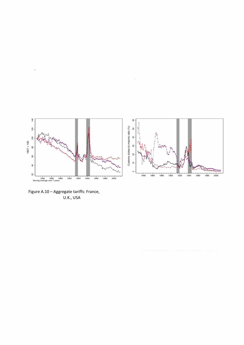
Moving average over 7 years

Figure A.10 – Aggregate tariffs: France, U.K., USA

Figure A.13 – P-values of the Breusch-Pagan test for the OLS estimation of

equation (15)

Internal trade = Gross output minus exports (benchmark) Internal trade = Gross tradable output minus exports

The shaded areas represent 95% confidence intervals Standard errors clustered at the bilateral level

Figure A.14 – Tariff-equivalent border

effect: OLS vs. PPML estimation

ε = -5.03 (benchmark) ε = -3 ε =

-7 (as in Jacks et al., 2008)

Figure A.15 – World trade cost indices with

alternative measures of internal trade,

restricted samples

Figure A.16 – Tariff-equivalent border

effect: Alternative trade elasticities

Figure A.17 – Import shares from the Netherlands, by distance