DIVERSIFICATION THROUGH TRADE∗

Francesco Caselli† Miklós Koren‡ Milan Lisicky§

Silvana Tenreyro†

Final Version: September 2019

Abstract

A widely held view is that openness to international trade leads to higher income

volatility, as trade increases specialization and hence exposure to sector-specific shocks.

Contrary to this common wisdom, we argue that when country-wide shocks are impor-

tant, openness to international trade can lower income volatility by reducing exposure

to domestic shocks, and allowing countries to diversify the sources of demand and sup-

ply across countries. Using a quantitative model of trade, we assess the importance

of the two mechanisms (sectoral specialization and cross-country diversification) and

show that in recent decades international trade has reduced economic volatility for

most countries.

∗Thanks: Referees, Pol Antras, Costas Arkolakis, Robert Barro, Fernando Broner, Ariel Burstein, LorenzoCaliendo, Julian DiGiovanni, Bernardo Guimaraes, Nobu Kiyotaki, Pete Klenow, David Laibson, FabrizioPerri, Steve Redding, Ina Simonovska, Jaume Ventura, Romain Wacziarg, and seminar participants atBocconi, Birmingham, CREI, Princeton, Penn, Yale, NYU, UCL, LBS, LSE, Toulouse, Warwick, as well asparticipants at SED, ESSIM, and the Nottingham trade conference. Calin Vlad Demian, Balazs Kertesz,Federico Rossi, and Peter Zsohar provided superb research assistance. Caselli acknowledges financial supportfrom the Luverlhume Fellowship. Koren acknowledges financial support from the European Research Council(ERC) starting grant 313164. Tenreyro acknowledges financial support from the ERC starting grant 240852.† London School of Economics, CfM, CEPR. ‡ Central European University, MTA KRTK, CEPR. § EuropeanComission. Correspondence: s.tenreyro@LSE.ac.uk.

1

I Introduction

An important question at the crossroads of macro-development and international economics

is whether and how openness to trade affects macroeconomic volatility. A widely held view

in academic and policy discussions, which can be traced back at least to Newbery and

Stiglitz (1984), is that openness to international trade leads to higher income volatility. The

origins of this view are rooted in a large class of theories of international trade predicting

that openness to trade increases specialization. Because specialization in production tends

to increase a country’s exposure to shocks specific to the sectors (or range of products) in

which the country specializes, it is generally inferred that trade increases volatility. This view

seems present in policy circles, where trade openness is often perceived as posing a trade-off

between the first and second moments (i.e., trade causes higher productivity at the cost of

higher volatility).1

This paper revisits the common wisdom on two conceptual grounds. First, the existing

wisdom is strongly predicated on the assumption that sector-specific shocks (hitting a par-

ticular sector) are the dominant source of income volatility. The evidence, however, does

not support this assumption. Indeed, country-specific shocks (shocks common to all sectors

in a given country) are at least as important as sector-specific shocks in shaping countries’

volatility patterns (e.g. Stockman, 1988, Costello, 1993, Koren and Tenreyro, 2007).2 The

first contribution of this paper is to show analytically that when country-specific shocks are

1See for example the report on “Economic openness and economic prosperity: trade and investmentanalytical paper”(2011), prepared by the U.K. Department of International Development.

2Both Stockman and Costello find that country-specific shocks are more important than sector-specificshocks in shaping volatility patterns in seven (resp., five) industrialized countries. Using a wider sample ofcountries and a different method, Koren and Tenreyro confirm these results, and find that the relative weightof country-specific shocks is even more relevant in less developed economies.

2

an important source of volatility, openness to international trade can lower income volatility.

In particular, openness reduces a country’s exposure to domestic shocks, and allows it to

diversify its sources of demand and supply, leading to potentially lower overall volatility.

This is true as long as the volatility of shocks affecting trading partners is not too large, or

the covariance of shocks across countries is not too large. In other words, we show that the

sign and size of the effect of openness on volatility depends on the variances and covariances

of shocks across countries.

Second, the paper questions the mechanical assumption that higher sectorial specializa-

tion per se leads to higher volatility. Indeed, whether income volatility increases or decreases

with specialization depends on the intrinsic volatility of the sectors in which the economy

specializes in, as well as on the covariance among sectorial shocks and between sectorial and

country-wide shocks.

We make these points in the context of a quantitative, multi-sector, stochastic model

of trade and GDP determination. The model builds on a variation of Eaton and Kortum

(2002), Alvarez and Lucas (2007), and Caliendo and Parro (2015), augmented to allow for

country-specific and sector-specific shocks.3 In each sector, production combines equipped

labour with a variety of tradable inputs. Producers source tradable inputs from the lowest-

cost supplier (where supply costs depend on the supplier’s productivity as well as trade

costs), after productivity shocks have been realized. This generates the potential for trade

3Variations of this model have been used to address a number of questions in international economics. Anincomplete list includes Hsieh and Ossa (2011) and di Giovanni, Levchenko, and Zhang (2014), who study theglobal welfare impact of China’s trade integration and technological change; Levchenko and Zhang (2013),who investigate the impact of trade with emerging countries on labour markets; Burstein and Vogel (2016)and Parro (2013), who study the effect of international trade on the skill premium; Caliendo, Parro, Rossi-Hansberg and Sarte (2014), who study the impact of regional productivity changes on the U.S. economy,and so on. None of these applications, however, focuses on the impact of openness to trade on volatility. Apartial exception is Burgess and Donaldson (2012), which we discuss below.

3

to “insure”against shocks, as producers can redirect input demand to countries experiencing

positive supply shocks. However, (equipped) labor must be allocated to sectors before pro-

ductivity shocks are realized. This friction allows us to capture the traditional specialization

channel, because it reduces a country’s ability to respond to sectorial shocks by reallocating

resources to other sectors. An extension of the model allows for ex-post sectorial reallocation

of equipped labour in the presence of reallocation costs.

We use the model in conjunction with production and bilateral trade data for 24 sectors

and a diverse group of 25 countries to quantitatively assess how changes in trading costs

have affected income volatility between 1972 and 2007.4 We find that the decline in trade

costs since the 1970s has caused sizeable reductions in income volatility in the vast majority

of the countries in our sample. On average, volatility fell 36% compared to a counterfactual

where trade barriers remain at their early-1970s level. The range of changes in volatility due

to trade varies significantly across countries, with the largest reductions being in the order

of 80%.

The general decline in volatility due to trade is the net result of the two different

mechanisms discussed above: sectorial specialization, and country-wide diversification. The

country-wide diversification mechanism again contributed to lower volatility in most of the

countries in our sample, consistent with our key idea that trade is a source of diversification

of country-wide shocks. On the other hand, the sectoral-specialization mechanism increased

volatility in only just above one half of the countries in the sample. Consistent with our theo-

retical points above, then, the common wisdom that specialization leads to greater volatility

fails to apply almost as often as it does. The crucial and most important point, however, is

4We stop the analysis in 2007 as our model abstracts from the factors underlying the financial crisis.

4

that the country-wide diversification effect is on average eight times as large as the sectoral-

specialization effect, so that the net effect is that trade reduces volatility in the overwhelming

majority of cases.

We subject our results to a variety of robustness checks and extensions. In the latter,

we find that it is important to feature a detailed input-output structure to fully capture the

impact of trade on volatility. We also find that the impact of trade on volatility is not driven

by the emergence of China, but it is a much more general phenomenon.

The focus of our quantitative evaluation is real income, defined as nominal GDP deflated

by a cost of living index. In the model, the cost of living index is a preference-based ideal

price deflator. In the data counterpart, the cost of living index is the CPI. Hence, we work

with a welfare-relevant notion of income.5

Since our focus is the volatility of income, we abstract from trade in financial assets.

Trade in financial assets has important potential implications for consumption volatilty (as

it allows for consumption-risk sharing) but not for income volatility, which is driven by the

production side of the economy. Having said that, for most countries in the world income

and consumption fluctuations are very highly correlated, so that consumption-risk sharing

via asset trade does not appear to be empirically significant anyway.6 ,7

5Kehoe and Ruhl (2008) and Burstein and Cravino (2015) study the theoretical impact of foreign pro-ductivity shocks on various measures of domesitc economic activity. In general, foreign productivity shocks(or other sources of change in the terms of trade) have little first-order effects on production-based measuresof activity (e.g. GDP deflated by the GDP deflator), while they have first-order effects on welfare-basedmeasures.

6For recent contributions showing that risk sharing seems quite limited empirically, especially outside ofa small number of rich economies, see, e.g., Ho and Ho (2015), Hevia and Servén (2018), Fuleky et al (2017),Rangvid et al. (2016).

7Fitzgerald (2012) points out that lowering trade costs for goods also reduces the costs of trade in assets,increasing consumption risk sharing and lowering consumption volatility. Along similar lines, Reyes-Heroles(2017) argues that lower trade costs leads to more inter-temporal trade. Because we do not allow for assettrrade these effects of lower trade costs are not present in our model.

5

The fact that openness to trade has ambiguous predicted effects on volatility might

partly explain why direct empirical evidence on the effect of openness on volatility has

yielded mixed results. Some studies find that trade decreases volatility [e.g., Bejan (2006),

Buch, Döpke and Strotmann (2009), Cavallo (2008), Haddad, Lim and Saborowski (2010),

Parinduri (2011), Burgess and Donaldson (2012)], while others find that trade increases

it [e.g., Rodrik (1998), Easterly, Islam, and Stiglitz (2001), Kose, Prasad, and Terrones

(2003), di Giovanni and Levchenko (2009)]. The model-based analysis can circumvent the

problem of causal identification faced by many empirical studies, allowing for counterfactual

exercises that isolate the effect of trade costs on volatility. Moreover, it can cope with highly

heterogenous trade effects across countries.

Besides contrasting with assessments of the trade-volatility relationship based on (a sim-

plistic understanding of) the specialization framework, our paper also offers an alternative

perspective on openness and volatility to the so-called International Real Business Cycle

approach. Backus, Kehoe, and Kydland (1992) show that GDP volatility is higher in the

open economy than in the closed economy, as capital inputs are allocated to production

in the country with the most favorable technology shock. Hence, income fluctuations are

amplified in an open economy. In our multi-country, multi-sector setting, instead, income

volatility can– and often does– decrease with openness, as intra-temporal trade in inputs

allows countries with less favorable productivity shocks to source inputs from abroad, thus

reducing income (as well as consumption) volatility.8

8Also related is the empirical literature initiated by Frankel and Rose (1998), who documented a strongcorrelation between bilateral trade flows and GDP comovements between pairs of countries (see also, e.g.,Kose and Yi (2001), Arkolakis and Ramanarayanan (2009)). Our main focus in this paper is on the effectof trade on volatility– and the channels mediating this effect– but the quantitative approach we follow inour counterfactual exercises can potentially be extended to also identify the effect of trade on bilateralcomovement– and indeed, other higher-order moments.

6

A paper that is closely related to ours is Burgess and Donaldson (2012), who use the

Eaton-Kortum model in conjunction with data on the expansion of railroads across regions in

India to assess whether real income became more or less sensitive to rainfall shocks, as India’s

regions became more open to trade. The authors find that the decline in transportation costs

lowered the impact of productivity shocks on real income, implying a reduction in volatility.

Our analysis is at a higher level of generality, and highlights that, while a reduction in

volatility has been experienced by many countries as they became more open to trade, the

size and sign of the trade effect on volatility may be– and indeed has been– different across

different countries.9

While this paper focuses on contrasting our new diversification-through-trade mechanism

with the traditional sectoral specialization mechanism, it leaves to future work to include the

role of “granular”shocks. As pointed out by di Giovanni and Levchenko (2012), if openness

to trade increases concentration, the impact of granular shocks is exacerbated, potentially

leading to an increase in volatility. See also di Giovanni, Levchenko and Mejean (2014) for

a country-level application.

The remainder of the paper is organized as follows. Section II presents the model and

solves analytically for two special cases, autarky and costless free trade. Section III introduces

the data and calibration. Section IV presents the quantitative results, including robustness

checks and extensions. Section V presents concluding remarks. The Appendix contains

further derivations and a detailed description of the data sets used in the paper.

9See also Donaldson (2015), where the question is also addressed in the context of India’s railroad ex-pansion. There is also a growing literature on the effect of globalization on income risk and inequality. Wedo not focus on distributional effects within countries in this paper, though it is obviously a very importantissue, and a natural next step in our research. For theoretical developments in that area, see, for example,Anderson (2011) and the references therein.

7

II A Model of Trade with Stochastic Shocks

The baseline model builds on a multi-sector variation of Eaton and Kortum (2002), Alvarez

and Lucas (2006), and Caliendo and Parro (2015), augmented to allow for stochastic shocks,

as well as frictions to the allocation of non-produced (and non-traded) inputs across sectors.

II.A Model Assumptions

The world economy is composed of N countries. In each country n there is a final con-

sumption good. The consumption good is a bundle of sectoral goods produced by J sectors.

In turn, each sectoral output is a bundle of sector-specific varieties. Each sectoral variety

can be produced domestically or imported. Domestic production of sectoral varieties uses

non-produced inputs, to which we refer to as “equipped labor,” and other sectoral goods

acting as intermediates. All markets are perfectly competitive.

The consumption bundle Cnt is packaged by a consumption-good producer using the

Cobb-Douglas aggregate

Cnt =∏J

j=1

(Cjnt

)αjt , (1)

where Cjnt is the quantity of sectoral good j used for consumption, and

∑Jj=1 α

jt = 1. The

αs are allowed to change over time to capture possible changes in tastes. In Section IV.B.4

we investigate the robustness of our results to a specification of preferences in which the

elasticity of substitution among sectoral goods is not unitary.

Sectoral output in sector j, Qjnt, is

Qjnt =

[∫ 1

0

qnt(ωj)

η−1η dωj

] ηη−1

, (2)

8

where qnt(ωj) is the quantity of sectoral variety ωj used in sector j, and η > 0 is the

elasticity of substitution across goods within a given sector. Implicit in this formulation is

the assumption that each sector relies on a continuum of sector-specific varieties, ωj.

The technology for producing good ωj in country n is

xnt(ωj) = Ajntzn(ωj)lnt(ω

j)βj∏J

k=1Mk

nt(ωj)γ

kj

, (3)

where xnt(ωj) is the output of good ωj by country n at time t; Mknt(ω

j) is the amount of

sector k output used by country n in the production of good ωj; lnt(ωj) is the corresponding

amount of equipped labour; zn(ωj) is a time-invariant variety-specific productivity factor;

and Ajnt is a time-varying productivity shock common to all the varieties in sector j. The

exponent γkj captures the share of sector k in the total production cost of sector j. We

assume constant returns to scale, or βj +∑J

k=1 γkj = 1, for all j. Notice that (3) allows

for a rich input-output structure, as the intensity with which each sector’s output is used as

intermediate by other sectors varies across all sector pairs.

Building on the literature, we assume that the productivities zn(ωj) follow a sector-

specific, time-invariant Fréchet distribution F jn(z) = exp(−T jnz−θ). A higher T jn shifts the

distribution of productivities to the right, leading to probabilistically higher productivities.

A higher θ decreases the dispersion of the productivity distribution, and hence reduces the

scope for comparative advantage. The z terms are the main determinants of long-term

comparative advantage in our model.

The shocks to Ajnt over time are interpreted as standard TFP shocks, and make the

model stochastic at the aggregate level. We will later decompose them into a country-

9

specific component and a sector-specific component. This decomposition will be used to

identify separately the country diversification and the sectoral specialization channels.

The intermediate goods ωj can be produced locally or imported from other countries.

Delivering a good from country n to country m in sector j and time period t results in

0 < κjmnt ≤ 1 goods arriving at m; we assume that κjmnt ≥ κjmktκjknt ∀m,n, k, j, t and

κjnnt = 1. All costs incurred are net losses.10 Under the assumption of perfect competition,

goods are sourced from the lowest-cost producer, after adjusting for transport costs. The

sectoral outputs Qjnt are nontraded.

At a given point in time t, country n is endowed with Lnt units of a primary (non

produced) input, which we interpret as equipped labour. At the beginning of each period,

before the realization of the shocks Ajnt, a representative consumer decides on the optimal

allocation of the primary input Lnt across the different sectors, Ljnt. After the shocks to

productivity are realized, equipped labour can be reallocated within a sector, but not across

sectors. Next, production and consumption take place. Clearing in the input market within

a sector implies

Ljnt =

∫ 1

0

lnt(ωj)dωj.

The lack of ex-post reallocation across sectors in a given period aims at capturing the

idea that in the short run it is costly to reallocate productive factors across sectors. Aside

from realism, our main intention in including it is that we wish to nest into our model

the traditional view that trade causes volatility by pushing countries to specialize - thus

10In the calibration, the κs will reflect all trading costs, including tariffs. Hence, implicitly we adopt theextreme assumption that tariff revenues are wasted– or at least not rebated back to agents in a way thatwould interact with the allocation of resources in the economy.

10

making them overly responsive to sectoral shocks. Without frictions to sectoral reallocation,

this mechanism could not arise, as the economy would respond to shocks by moving labor

from the negatively-affected sectors to the sectors receiving (relatively) positive shocks. Our

model would then feature only our novel mechanism, namely the diversification of country-

level shocks.11

The representative agent has a per-period utility flow log(Cnt).12 Because there is no

(endogenous) intertemporal trade and no capital in the economy, the only decision the rep-

resentative agent has to take in each period is the allocation of equipped labor across sectors

before observing the shock realizations. Since labor can be freely reallocated at the beginning

of each period, this is a purely static decision.

Since equipped labor is the only non-produced input, the per period budget constraint

in each period is:

PntCnt =∑J

j=1wjntL

jnt (4)

where Pnt is the price of the consumption good defined in equation (1), and wjntL

jnt is the

nominal value-added generated in sector j. This budget constraint assumes that trade is

balanced. In Section IV.B we relax this assumption.

Using (4) in the utility function we can solve for the sectoral labor allocation:

Ljnt = arg maxEt−1

[log

(∑Jj=1w

jntL

jnt

Pnt

)], s.t. :

∑J

j=1Ljnt = Lnt, (5)

11In the quantification, a period will be one year. This amounts to assuming that it takes at least one yearfor resources to be reallocated across sectors. In Section V we relax the assumption of full rigidity withinone period, and allow for ex post sectoral reallocation of equipped labour subject to an adjustment cost,which we calibrate to match sectoral reallocation flows in the data.12The log utility assumption gives rise to a particularly intutive and tractable decision rule for the labor

allocation.

11

where Et−1 indicates the rational expectation over the possible realizations of period t shocks.

In particular, the representative agent at the beginning of time t knows the previous values

of the shock processes Ajnt−1, as well as the distribution of Ajnt conditional on A

jnt−1 (which

we specify in Section III.A.4), and is therefore able to compute the rational expectation in

(5).

Note that the model above implictly assumes that producers can switch suppliers rel-

atively easily in response to shocks. Since we later calibrate a period to one year, we are

saying that firms can react to problems with one supplier by finding another source within

12 months of the shock. The trade literature does suggest considerable churning on the ex-

tensive margin. For example, Bernard, Jensen, Redding, and Schott (2009) document that

changes in the set of products and countries that firms source from account for between

1/3 and 1/2 of annual import fluctuations. Furthermore, much of the diversification bene-

fits can accrue at the intensive margin: firms build a diversified portfolio of suppliers, and

then use the intensive margin vis-à-vis each supplier to absorb shocks —i.e. increasing the

volumes from suppliers experiencing a positive shock and reducing volumes from suppliers

experiencing a negative shock. Cadot, Carriere, and Strauss-Kahn (2014) find evidence of

increased diversification of suppliers among OECD firms. Paid consultants give open advice

on diversification of suppliers as a way to protect firms from shocks.13

13E.g. https://www.exostar.com/blog/can-supply-chain-diversification-reduce-risk/ andhttps://www.ideasforleaders.com/ideas/supply-chain-risk-diversification-vs-under-diversification.

12

II.B Model Solution

Conditional on the realization of the country-and-sector specific shocks Ajnt, our model is

very similar to other general equilibrium, multi-sector versions of the Eaton-Kortum model.

The main difference is that equipped labor is pre-allocated across sectors. Hence, we do

not offer a detailed derivation of the key equilibrium conditions that are unaffected by the

ex-ante allocation of resources, but merely state them in the following list.

djnmt =

T jm

(Bj(wjmt)

βj ∏Jk=1(Pkmt)

γkj

Ajmtκjnmt

)−θ∑N

i=1 Tji

(Bj(wjit)

βj ∏Jk=1(Pkit)

γkj

Ajitκjnit

)−θ , (6)

P jnt = ξ

N∑m=1

T jm

Bj(wjmt

)βj∏Jk=1(P k

mt)γkj

Ajmtκjnmt

, (7)

Pnt =∏J

j

(1

αjn

)αj (P jnt

)αj, (8)

Rjnt =

∑N

m=1djmntE

jmt, (9)

Ejnt = αjtPntCnt +

∑J

k=1γjkRk

nt, (10)

wjntLjnt = βjRj

nt, (11)

and the budget constraint (4). In the equations above, djnmt is the fraction of country n’s

total spending on sector-j goods that is imported from countrym; P jnt is the price of sectoral-

good j in country n; Rjnt is total revenues accruing to firms operating in sector j in country

n; and Ejnt is total expenditure by country n residents (consumers and firms) on sectoral

13

good j. Bj ≡(βj)−βj J∏

k=1

(γkj)−γkj

and ξ ≡ Γ(θ+1−ηθ

), where Γ is the gamma function, are

parametric constants. Hence, equation (6) says that country n imports disproportionately

from countries m and sectors j that have high productivity draws T jm and Ajmt; low wages

wjmt and sectoral prices Pkmt; and low bilateral trading costs, namely high κnmts. Equation

(7) says that the same factors affect domestic sectoral prices. Equation (8) follows from the

final-good producer’s profit maximization problem, and shows the price of consumption as an

aggregate of the sectoral prices. Equation (9) expresses the total sales of sector j in country

n as a function of each country’s expenditures on that sector and the share of country n in

each country’s imports in that sector. Equation (10) states that a country’s expenditures in

sector j is the sum of final and intermediate uses of sector j goods. Equation (11) simply

notes from the Cobb-Douglas formulation that value added from sector j is a share βj of the

gross output of sector j.

To these fairly standard equilibrium conditions we add here the first-order conditions for

the allocation of inputs to sectors, i.e. the solution to (5). This turns out to be:

LjntLnt

= Et−1

[wjntL

jnt∑

k wkntL

knt

], ∀j, t. (12)

The share of resources allocated to a given sector equals its expected share in value added.

Note that 1/∑

k wkntL

knt is the marginal utility of consumption in period t; thus, more re-

sources are allocated to higher value-added sectors, after appropriately weighting by marginal

utility.14

14Compared to the allocation in a determinisitc model, in our stochastic application sectors whose pro-ductivity is negatively correlated with aggregate productivity (that is, they have high value added when therest of the economy has low value added) are allocated a disproportionate share of resources. In states of

14

The model can conceptually be solved backwards in two steps. First, for any given set of

values for Ljnt, equations (6)-(11) can be solved for Pnt, wjnt, P

jnt, d

jnmt, E

jnt, R

jnt, and Cnt as

functions of the κjmnts, the Tjnts, the A

jnts, and of course the L

jnts. For calibration purposes

it turns out to be both possible and convenient to express the dependence of these solutions

on T jn, Ajnt, and L

jnt in terms of the augmented productivity factors

Zjnt ≡ T jn

(Ajnt)θ

(Lnt)βjθ (13)

and the sectoral employment shares LjntLnt. The augmented productivity factors capture the

joint influence of all the exogenous processes (whether deterministic or stochastic) that im-

pinge on the country and sector overall productive capacity.

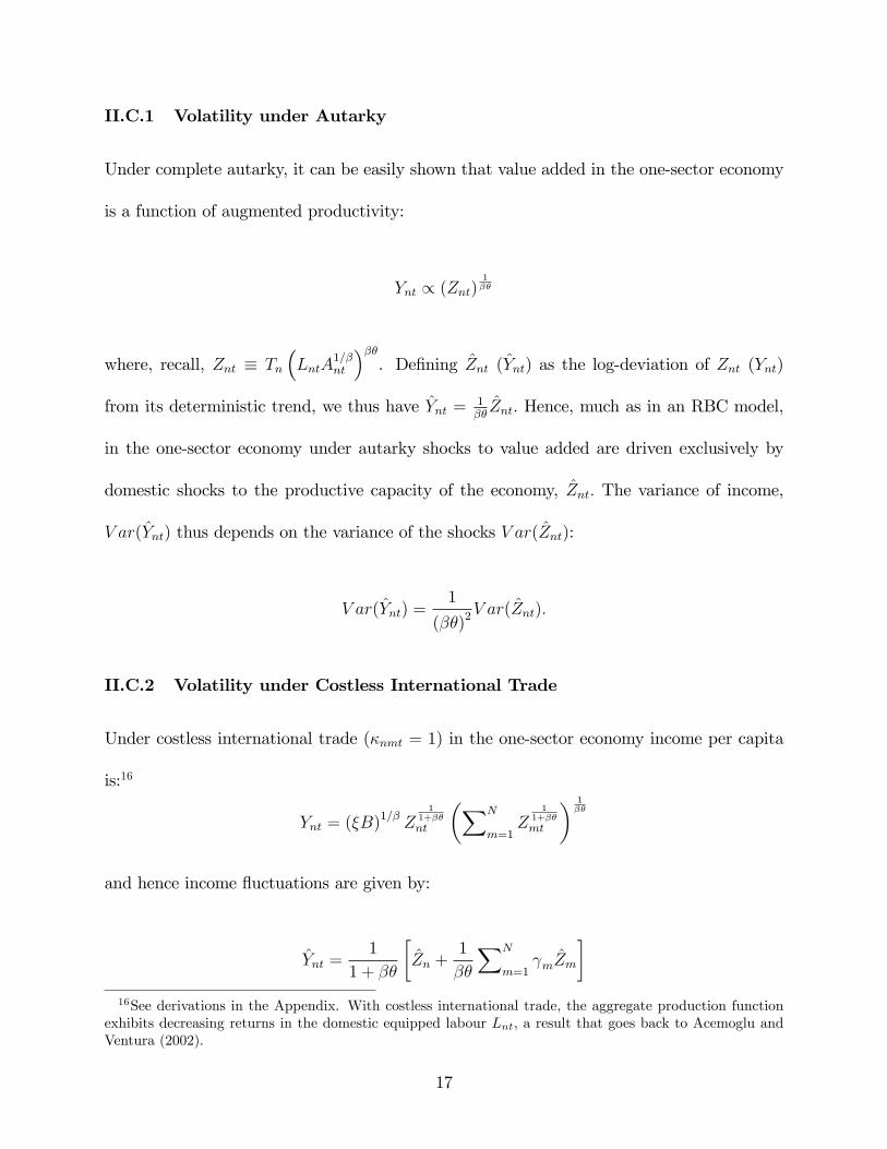
The second stage of the solution uses (12) to find the ex-ante shares Ljnt/Lnt. Our solution

method computes the rational expectation in (12) by drawing from the estimated distribution

of Ajnt. In particular, we begin with a choice of candidate values for the Ljnts, and draw a

large number of realizations of the Ajnts from their estimated distributions (conditional on the

Ajnt−1s). For each of these realizations, we compute the solution for the wjnts from the system

(6)-(11), and then the term in brackets on the right side of (12). The rational expectation is

then the average of the terms in brackets across all the simulated realizations. If this is (close

enough to being) equal to the starting guess for Ljnt/Lnt the algorithm stops. Otherwise, it

moves to a new guess for Ljnt/Lnt. A more detailed explanation is provided in the Appendix.

The key theoretical outcome we are interested in is aggregate income volatility, which we

measure as the variance (or standard deviation, where indicated), of real income deviations

the world in which overall income is low, the marginal utility of consumption 1/∑

k wkntL

knt will be high and

hence the optimal allocation entails allocating more resources to this sector.

15

from country-specific trends. In turn, real income in the model is given by total value added

deflated by the optimal expenditure-based price index, or Ynt = wntLntPnt

. As discussed in

the Introduction, these welfare-relevant measures of income are expected to show first-order

responses to changes in the terms of trade, and hence in foreign productivities, endowments,

or trade costs.15

II.C Two Illustrative Cases: Autarky and Costless Trade

To illustrate our novel mechanism of diversification through trade, we begin by analyzing

a one-sector version of the model (that is, the original Eaton-Kortum model) under two

extreme cases for which we have closed-form analytical solutions: autarky (κnmt = 0 for

all n 6= m, t) and costless trade (κnmt = 1 for all n,m, t). We accordingly drop the sector

subscripts. The final good is still used as an intermediate. Note that in both cases we can set

Pn = 1 for all n. In the autarky case this is an innocuous normalization. In the costless-trade

case this is due to the fact that prices are equalized across countries.

15In contrast, if we were to deflate nominal GDP by using the CES price aggregates of the sector-levelvariety baskets, we would retrieve the Kehoe-Ruhl invariance of GDP to shocks to the terms of trade. It isdoubtful, however, that GDP as constructed by statistical agencies maps well into this theoretical construct.They may measure the price of a representative variety within each sector, the average price of an aggregatevariety basket, or a random sample of continuously used varieties. This choice might also depend on thesource country, as import price indexes are computed differently from producer price indexes (Nakamuraand Steinsson, 2008 and Nakamura and Steinsson, 2012). In contrast, the CPI is easier to map to ourmodel, because consumers only consume J different final goods, not a continuum of varieties. Our welfare-relevant price index, which is the geometric average of final good prices is a very close approximation of theexpenditure-weighted Törnqvist price index, the way the CPI is usually calculated.

16

II.C.1 Volatility under Autarky

Under complete autarky, it can be easily shown that value added in the one-sector economy

is a function of augmented productivity:

Ynt ∝ (Znt)1βθ

where, recall, Znt ≡ Tn

(LntA

1/βnt

)βθ. Defining Znt (Ynt) as the log-deviation of Znt (Ynt)

from its deterministic trend, we thus have Ynt = 1βθZnt. Hence, much as in an RBC model,

in the one-sector economy under autarky shocks to value added are driven exclusively by

domestic shocks to the productive capacity of the economy, Znt. The variance of income,

V ar(Ynt) thus depends on the variance of the shocks V ar(Znt):

V ar(Ynt) =1

(βθ)2V ar(Znt).

II.C.2 Volatility under Costless International Trade

Under costless international trade (κnmt = 1) in the one-sector economy income per capita

is:16

Ynt = (ξB)1/β Z1

1+βθ

nt

(∑N

m=1Z

11+βθ

mt

) 1βθ

and hence income fluctuations are given by:

Ynt =1

1 + βθ

[Zn +

1

βθ

∑N

m=1γmZm

]16See derivations in the Appendix. With costless international trade, the aggregate production function

exhibits decreasing returns in the domestic equipped labour Lnt, a result that goes back to Acemoglu andVentura (2002).

17

where γm = Z1

1+βθm∑N

i=1 Z1

1+βθi

is the relative size of country j evaluated at the mean of Zjs. Re-

arranging, we obtain Ynt = 1βθ

[γn+βθ1+βθ

Zn + 11+βθ

∑Nm 6=n γmZm

]. Volatility under free trade is

hence given by:

V ar(Ynt) =

(1

βθ

)2

(γn+βθ1+βθ

)2

V ar(Znt) +[

11+βθ

]2∑m 6=i γ

2mV ar(Zmt)

2γn+βθ1+βθ

11+βθ

∑m6=n γmCov(Zm,Zn)

Compared to the variance in autarky, 1

(βθ)2V (Znt), it is clear that the volatility due to

domestic productivity fluctuations, V ar(Znt), now receives a smaller loading, as(γn+βθ1+βθ

)2

<

1 since γn < 1. The smaller the country (as gauged by its share γn), the smaller the impact

of domestic volatility of shocks, Zn, on its income, when compared to autarky. Openness to

trade, however, exposes the economy to other countries’productivity shocks, which will also

contribute to the country’s overall volatility.

Whether or not the gain in diversification (given by lower exposure to domestic pro-

ductivity) is bigger than the increased exposure to new shocks depends on the variance-

covariance matrix of shocks across countries. If all countries have the same constant variance

V ar(Znt) = σ, and the Znt are uncorrelated, volatility under free trade becomes:

V ar(Ynt) =

(1

βθ

)2{(

γn + βθ

1 + βθ

)2

+

[1

1 + βθ

]2∑m 6=i

γ2m

}σ

which is unambiguously lower than the volatility under autarky.17 Of course, if other coun-

tries have higher variances or the covariance terms are important, then the weights countries

17To see this note that 2βθγn +∑

j=1 γ2j < 2βθ + 1 since γm ≤ 1 for every m, and so (βθ)

2+ 2βθγn +∑

j=1 γ2j < (1 + βθ)2. This means that the expression in curly brackets is less than 1.

18

receive matter and the resulting change in volatility cannot be unambiguously signed.

Aside from the over-simplified variance and covariance structure, these examples abstract

from the traditional channel thought to link trade to increased volatility, namely sectoral

specialization. In order to evaluate the relative importance of country diversification and

sectoral specialization, as well as to base the analysis on a more realistic stochastic environ-

ment based on the data, and to evaluate inframarginal changes in trade costs, the rest of

the paper focuses on the full multi-sector model with frictions to the reallocation of labor

following the realization of shocks.

III Quantification

Our goal is to quantitatively assess the effect of historical changes in trade barriers on income

volatility for as large a sample of countries and as fine a level of sectoral disaggregation as

available data allows. It turns out that the necessary data are available for a sample of

24 core countries, and an aggregate of the remaining countries, to which we refer to as

“rest of the world”(ROW). The country coverage is good, in the sense that the countries

included account for an overwhelming share of world GDP and trade. In terms of sectoral

breakdown, we are able to consider 24 sectors: agriculture, 22 manufacturing sectors, and

services. It would clearly have been desirable to access an even finer breakdown. Among

other things, a finer breakdown would have potentially implied greater effective rigidity in

the allocation of labor across sectors, allowing us to test the robustness of our conclusions

on the importance of the specialization channel. Nevertheless, 24 sectors is at the top end of

the level of disaggregation usually achieved in applications of the Eaton-Kortum framework.

19

In order to solve the model numerically, we need to estimate the values of the exogenous

trading costs κjnmt and the augmented productivity processes Zjnt. We also need to calibrate

the parameters αjt , βj, γkj, θ, and η.

III.A Exogenous Processes

As has become standard in empirical applications of the Eaton and Kortum framework, we

back out realized paths of both trade costs κjnmt and augmented productivities Zjnt from (ver-

sions of) the gravity equation (6) [e.g. Costinot, Donaldson, Komunjer (2012), Levchenko

and Zhang (2014, 2016)]. Allen, Arkolakis, and Takahashi (2017) discuss the identification

issues involved in this inference problem, whose solution generally requires additional in-

formation on trade costs. In our case, we impose additional restrictions on the patterns of

bilateral trade costs, which allow us to back out the full matrix of bilateral trade costs κjnmt

independently from the Zjnts. We can then plug the estimated κ

jnmts back into (6) to back

out the Zjnts.

18

III.A.1 Trade Costs

In order to back out the κjnmts independently of the other variables in the gravity equation

we follow Head and Ries (2001) and assume that κjnmt = 1 for n = m, and that κjnmt = κjmnt

for all n, m, and j. With these assumptions, equation (6) can be manipulated to yield:

djnmtdjmnt

djmmtdjnnt

=(κjnmt

)2θ. (14)

18An alternative to our two-step strategy is to find proxies for the observable determinants of trade costs(e.g. distance, or colonial links) and model the κs explicitly as functions of these determinants. Thenequation (6) can be estimated econometrically and the Zs recoverd as (functions of) country-sector fixedeffects. See, e.g., Levchenko and Zhang (2014).

20

Recall that djnmt is the fraction of country n’s total spending on sector-j goods that is

imported from country m. Imports are directly observable and spending can be constructed

from available data as gross sectoral output plus sectoral imports minus sectoral exports.

Hence, for a given value of θ (see below for the calibration of this parameter), we can obtain

the time series of trading costs by sector and country-pairs{κjnmt

}.

Figure 1 shows the histograms of bilateral κs in manufacturing and agriculture in the first

and last year of our sample (recall that services are treated as a nontradable sector). In both

agriculture and manufacturing trade barriers have declined significantly since the early 1970s.

As is typical of estimated trade costs from gravity equations the levels of the trade costs

are very large. But it is important to remember that the trade barriers do not only reflect

transport costs and tariff and non-tariff trade barriers; but also that many manufacturing

and, especially, agricultural goods are not fully tradable (e.g. perishable products). They

may also pick up a home-bias effect that is not explicitly modelled in Eaton and Kortum.

III.A.2 Productivity in Tradable Sectors

Using again (6), together with (7) and our definition of augmented productivity (13), some

algebra yields

Zjnt = Bjθξθdjmnt

(wjntwnt

wntLnt

)θβj (κjmnt

)−θ∏J

k=1(P k

nt)θγkj

︸ ︷︷ ︸≡exp(ζjmnt)

(P jmt

)−θ. (15)

This equation holds for all n,m, j, t. It says that, for a given price of sectoral good j in

country m, P jmt, and bilateral trading costs κ

jmnt, productivity in country n in that sector is

21

inferred to be high if country n exports a lot to country m, or djmnt is large; aggregate value

added wntLnt is large, or if the sector has a high wjnt/wnt wage premium.

For all countries, we can directly observe several of the terms collected in the object we

have called exp(ζjmnt). In particular, data is available for sectoral import shares djmnt (as

already used in the previous subsection), nominal value added wntLnt, and aggregate prices

Pnt. We do not observe directly the sectoral wage premium wjnt/wnt, especially since w is

interpreted as the rental rate of equipped labor. To recover a series for the wage premium we

begin by rewriting the first order condition for the allocation of labor across sectors, equation

(12), as

wjntwnt

=wjntL

jnt/wntLnt

Et−1(wjntLjnt/wntLnt)

.

This says that a sector’s wage exceeds the average wage if its share in aggregate value added,

wjntLjnt/wntLnt, exceeds its expected share in aggregate value added. We directly observe each

sector’s share in aggregate value added - or the numerator. To compute expectations of the

value added share in the denominator, we use the (nonlinear) time trend of wjntLjnt/wntLnt.

We can check the validity of this procdure by comparing the trend of wjntLjnt/wntLnt with the

rational expectation of wjntLjnt/wntLnt in model-generated data. The correlation is 0.99 across

all countries, sectors,and time periods, and 0.94 after taking out country-sector means.19

This leaves us needing the sector-specific price deflators P jmt for some benchmark country

m. We could easily just plug into (15) the US sectoral price indices and use them to recover

the Zjnts for all other countries (and the US itself). It turns out, however, that in the next

subsection we will need sectoral price deflators for tradable sectors for all countries in order

19An alternative procedure would be to take a stand on the equipped-labor aggregate. For example,Levchenko and Zhang (2014) assume it is a Cobb-Douglas aggregate of capital and (raw) labor.

22

to obtain estimates of the productivity processes for the nontradable sector. As these sectoral

price indices are not available for many of the countries in our sample, we develop here a

procedure to back out tradeable prices. When we have tradable prices for all countries, we

can use (15) more effi ciently to estimate productivity processes.

Taking logs and rearranging (15) yields.

θ log(P jmt

)= ζjmnt − log

(Zjnt

).

Since this relationship (vis-a-vis) country n must hold for any generic countries m and m′,

we can write

θ log(P jmt

)− θ log

(P jm′t

)= ζjmnt − ζjm′nt.

Rearranging this, and averaging over n, we further get

θ log(P jmt

)=

1

N

∑N

n=1

(ζjmnt − ζjm′nt

)+ θ log

(P jm′t

).

Recalling that the ζs are observable for all n, this expression tells us that we can recover the

sectoral prices for any country m if we have sectoral price indices for at least one country

m′. We do have sectoral price indices for the US. We choose units of accounts for each sector

so that U.S. nominal sectoral prices are equal to 1 in 1972.

Having thus obtained sectoral price series P jmt for all countries and sectors, we can return

to (15) and recover Zjnt from

log(Zjnt) =

1

N

∑N

m=1

[ζjmnt − θ log

(P jmt

)].

23

Note that, in the last two expressions, instead of using the average across a country’s trade

partners we could have used any individual bilateral relation. Theoretically, either option is

valid. However, using the average minimizes the influence of measurement error.

III.A.3 Productivity in Nontradables

The procedure in the previous subsection uses data on trade flows and is thus only applicable

to the recovery of augmented productivities in the tradable sectors: agriculture and the

various manufacturing industries. To recover the productivity series in the service sector we

begin by constructing a time series for the price of services. From equation (8), the price of

services P sn,t can be written as

P snt =

(PntPUS,t

PUS,t

) 1αs (∏J

j=1αj−αj)− 1

αs[∏

j 6=s

(P jnt

)αj]− 1αs

.

We have just described in the previous subsection how to estimate the prices of all the

sectors other than services, i.e. the P jnts in the last term. From the Penn World Tables we

can obtain a general price index for each country n relative to the United States, PntPUS,t

. And

PUS,t is simply the US general price index. With the price series for services at hand, we

can construct augmented productivity in services, Zsnt using again equation (15), for the case

n = m (implying, therefore, dsmnt = κsmnt = 1).

III.A.4 Shock Processes

We assume that the recovered time series{

logZjnt

}are generated by a deterministc (trend)

component and a stochastic component. We identify the deterministic component of each

24

logZjnt with its band-pass filter. The stochastic component, which is the log-deviation from

this trend, is further decomposed into sector- and country-specific components, as in the

factor model described in Koren and Tenreyro (2007). In particular, and without loss of

generality, we decompose the cyclical component, denoted Zjnt =, as:

Zjnt = λjt + µnt + εjnt, (16)

where µnt is the country-specific factor, affecting all sectors within the country; λjt is the

global sectoral factor, affecting sector j in all countries; and the residual εjnt is the idiosyn-

cratic component, specific to the country and sector.20 In the counterfactual exercises, we can

mute the sector- or country-specific factors by setting the corresponding components equal

to 0, in order to identify the separate effects of the two trade channels affecting volatility.

Once we have recovered the historical series{λjt , µnt, ε

jnt

}we assume that they are generated

by AR(1) processes, and for each of them we estimate the autoregressive coeffi cient and the

variance.

When solving the model, and particularly equation (12), we assume that the represen-

20The three factors, λ, µ, and ε are estimated as:

λjt = N−1N∑n=1

Zjnt

µnt = J−1J∑j=1

αj(Zjnt − λ

jt

)εjnt = Zjnt − λ

jt − µnt,

where αj is the time average of sectoral expenditure shares αjt , and we impose the restriction∑

n µn = 0,implying that the country-specific effect is expressed relative to the world’s aggregate. We calculate thecountry factor as a weighted average of shocks, because the single sector of services takes up 70-80 percentof value added in many economies. This is in contrast to Koren and Tenreyro (2007), who use unweightedaverage. Their application focuses on manufacturing sectors, which do not differ as much in size.

25

tative agent fully knows the deterministic component of each logZjnt process, as well as the

autoregressive coeffi cients and variances of λjt , µnt, and εjnt. Furthermore, at the beginning

of each period t, the agent has observed all the realizations of λjt−1, µnt−1, and εjnt−1. With

this information, conditional on a candidate value of Ljnt/Lnt, he/she can form the rational

expectation in the right side of (12).

III.B Calibration

We set αjt so as to match the cross-country average of the share of sector j in total final

uses, in each year, using the data on value added described in the Appendix. The βjs are

calculated as the average ratios (across time and countries) of value added to total output in

each sector, again using the sectoral value added and gross output data from the appendix.

And the γkjs are the average shares of purchases by sector j from sector k from the OECD

input-output tables, as a share of total sectoral output.

We allow for a relatively broad parametric range for θ, from θ = 2 to θ = 8, consistent

with the estimates in the literature (see Eaton and Kortum, 2002, Donaldson 2015, and

Simonovska and Waugh, 2014). We use θ = 4 as the baseline case, and report the results

for other values when discussing the sensitivity of our results. We calibrate the elasticity

of substitution across varieties η = 4, consistent with Broda and Weinstein (2006)’s median

estimates. The results are not sensitive to this parametric choice.

26

IV The Effect of Trade on Volatility

This section uses the framework developed above to quantitatively assess how historical

changes in trade costs from the early 1970s have affected volatility patterns in a sample of

countries at different levels of development. We first analyze the baseline model’s results

and then perform a series of sensitivity checks and extensions.

IV.A Baseline Results

Figure 2 starts by comparing the baseline model-generated income volatility with the volatil-

ity in the data. The baseline model uses our benchmark calibration, θ = 4, and feeds in the

historical time series for the trade costs κmnt, and for the augmented productivity factors

Zjnt. The graph shows the standard deviation of real income deviations from trend. Recall

that real income is measured as value added deflated by the expenditure-based price index.

The data counterpart is nominal GDP deflated by the CPI index. The correlation between

volatility in the model and data series is 0.96 (0.88 without China) for the standard devi-

ation and 0.99 (0.89 without China) for the variance. The analysis that follows will focus

on the variance as a measure of volatility, rather than the standard deviation, because we

exploit the additivity properties of the former to separately account for the diversification

and sectoral-specialization effects.

Table 1 investigates how the changes in trading costs have affected volatility in the

24 countries in our sample (plus the rest of the world). Column 1 compares our baseline

scenario, which uses the estimated time paths of trading costs and productivity processes,

27

to a scenario in which we remove the secular decline in trading costs.21 In particular, in the

counterfactual scenario we keep all the κjnmts constant at their 1972 level. The column shows

volatility under the counterfactual minus volatility in the baseline, and this difference taken

as a percentage of the volatility at constant trading costs. The numbers can be interpreted

as the proportional change in volatility caused by the decline in trading costs.

The comparison in Column 1 reveals that volatility is generally higher under the coun-

terfactual scenario with constant trading costs than in the baseline. For all countries except

for China and the Rest of the World, there would have been more volatility under constant

trade costs than there actually was. For almost all countries, therefore, the common wisdom

which predicts greater volatility following trade integration does not seem to apply.

The biggest declines in volatility caused by trade occurred in Belgium-Luxemburg, Canada,

Denmark, Germany, Ireland, Mexico, the Netherlands, Spain, and the United Kingdom, all

of which saw volatility reductions due to trade in excess of 50% (meaning their volatility

has been 50 percent lower than it would have been had trading costs stayed at their 1972

levels). In the two countries-regions in which trade has created additional volatility, the

excess volatility is negligible. The (unweighted) average country in our sample experienced

a 36% decline in volatility thanks to increased openness. But this average effect masks a

huge amount of heterogeneity in the quantitative and qualitative effect of trade in volatility,

consistent with our discussion of the country-specificity of the trade-volatility relation.

As discussed at several points, openness affects volatility through two channels: a diversi-

fication effect and a specialization effect. While neither effect has an unambiguous impact, it

21The absolute numbers of the volatilities generated by the scenarios discussed in this Section are reportedin Appendix Table 1.

28

is sensible to expect the diversification effect to reduce the impact of country-specific shocks,

and hence - in most cases - to reduce volatility; similarly, by exacerbating the impact of

sectoral shocks, the specialization effect is generally deemed to increase volatility. In the rest

of the table we assess and quantify these predictions.

In order to quantify the impact of the diversification effect, we compare two counter-

factual scenarios. As before, the two scenarios differ in the path of trading costs, with one

scenario featuring the same decline in trading cost that we back out from the data, and

the other having trading costs constant at 1972 levels. However, in these two scenarios the

series for Zjnt is replaced by a modified series from which we remove all sectoral shocks (i.e.

the shocks λjt and εjt defined in Section III.A.4). In other words we ask what volatility

would have been with and without the observed decline in trade costs, if the only shocks to

productivity had been the country-wide shocks. Because these two scenarios do not feature

sectoral shocks, any differences in volatility must be ascribed to the diversification effect.

The difference is again expressed as a percentage of the volatility under the 1972’s trad-

ing cost levels and is reported in Column 2. Once again, overwhelmingly volatility at 1972

trade barriers is larger than volatility in the baseline case, confirming that the diversification

channel strongly operates in the direction of lower volatility - as expected. It is interest-

ing though that there are a few countries for which volatility is lower at 1972 trade costs.

As discussed, even the diversification channel can amplify volatility, if openness exposes a

country to disproportionately large and volatile trading partners, or partners whose shocks

are highly correlated with a country’s own. Evidently this was the case for these countries.

On average, the diversification channel induces a 41% drop in volatility relative to the case

where barriers are held at the initial value.

29

Because of the additive properties of the variance, the specialization effect can be quan-

tified as the difference between the overall change in volatility, and the change due to the

diversification effect. This is reported in Column 3. The figures should be interpreted as the

increased in volatility due to trade integration when only sectoralal shocks (global or country

specific) are present. The change is positive for 13 out of 25 countries. This is remarkable,

because according to the standard view the specialization channel should increase volatility

in the vast majority of cases. Evidently, there is a large number of countries which are

pushed to specialize into less volatile sectors, or into sectors that comove negatively (or less

positively) with the country’s aggregate shocks or other sectoral shocks. On average, the

specialization channel implies an increase in volatility of just 5%.

The most important lesson from the comparison of Columns 2 and 3 is about the relative

magnitude of the diversification and specialization effects. The average change due to the

diversification mechanism is about eight times as large, in absolute value, as the average

change due to the specialization mechanism. The specialization effect, on which the policy

debate seems centred, is not as important as the diversification effect. We have hinted at

the likely reason for this in the Introduction: country-specific shocks are simply much more

important quantitatively than sector-specific ones.

In Table 2 we briefly present a dynamic view of how the overall changes seen in Table 1

came about. As Table 1, the table presents comparisons of volatility under different scenarios,

but volatility is computed by decade.22 Not surprisingly, the impact of trade (understood

as the change in trading costs since 1972) on volatility is modest in the 1970s, as by the

22To calculate decadal volatility, we compute the variance of annual log growth rates in real GDP. It isinfeasible to estimate a band-pass filter given just 10 years of data. The overall magnitudes of volatility arevery similar to those in Table 1.

30

end of the 1970s trade costs had not had much time to drift away from the 1972 values.

Throughout the rest of the period, the gap between actual volatility and volatility at 1972

trade costs opens steadily, as the world economy becomes more and more integrated.

This overall monotonic decline in volatility, however, masks some more nuanced dynamics

of the diversification and specialization effects. In particular, the diversification effect peters

out in the period 2000-2007. This petering out in the last seven years of the sample may

possibly reflect some noisiness due to the relative short time span over which volatilities are

computed. However, taken at face value, it points to the fact that —consistent with our

theory —the impact of trade on volatility is not only heterogenous across countries, but also

over time. For example, the decline in the diversification effect could be due to country-wide

shocks becoming more correlated in the 2000s.

IV.B Sensitivity Analysis

In this section we evaluate the robustness of our baseline results to three alternative im-

plementation choices: (i) allowing for unbalanced trade; (ii) alternative calibration values;

(iii) allowing for costly labor reallocation across sectors, and (iv) allowing for elasticities of

substitution in consumption other than 1.

IV.B.1 Trade Imbalances

Our benchmark model focuses on the balanced trade case. Because we observe significant

trade imbalances during the sample period, we begin our robustness checks by allowing

countries to run trade surpluses and deficits. We do not attempt to endogenize trade deficits

as the computational challenges of adding intertemporal considerations (including issues of

31

default) are formidable. Furthermore, available theoretical models of intertemporal trade are

not particularly successful empirically. Hence, as is customary in quantitative applications

of the Eaton and Kortum model, we treat the trade surplus an as exogenous process which

we take from the data. The required modifications to the baseline model are described in the

Appendix. As shown in Table 3, the quantitative results with trade imbalances are extremely

similar to those in the baseline.

IV.B.2 Scope for Comparative Advantage θ

Table 4 shows the change in volatility due to international trade and its decomposition for

two other (extreme) values of θ, θ = 2 and θ = 8. The general message is qualitatively

robust: i) the effect of trade on volatility varies across countries; ii) the diversification

channel tends to reduce volatility; iii) sectoral specialization has pretty heterogenous effects

on volatility across countries; (iv) the diversification channel is much more important than

the specialization channel. Having said that, the magnitude of the effects is quite sensitive

to changes in θ, with the effect of trade on volatility being stronger for lower values of θ, i.e.

when the scope for comparative advantage increases.23

IV.B.3 Adjustment Costs and Ex Post Sectoral Reallocation

The baseline model assumes that the sectoral allocation of equipped labour is decided one

period in advance, before productivity shocks are realized. In this section we relax this stark

assumption. We assume that the ex post reallocation of equipped labour is possible, but

23This exercise underscores the importance of the parameter θ, and adds to the message of Arkolakis,Costinot, and Rodriguez-Clare (2012): in order to assess the effects of trade on key aggregate variables, theelasticity of trade to trade costs plays a key role.

32

an adjustment cost is paid in that reallocation. By making sectoral reallocation of labor

more flexible we necessarily reduce the importance of the sectoral specialization effect, and

magnify the relative importance of our novel diversification mechanism.

We model the cost of labor reallocation in reduced-form fashion. In particular, lifetime

utility is given by

Un =∞∑t=0

δt

{log(Cnt)−

%

2

J∑j=1

[ψjnt+ − ψ

jnt−

]2}, (17)

where ψjnt− =Ljnt−Lnt

and ψjnt+ =Ljnt+Lnt

, and Ljnt− (Ljnt+) is the equipped labour assigned to

sector j before (after) observing the realization of the shocks. A higher value of % implies

higher adjustment costs.

The ex-post sectoral input allocation solves:

Lknt+ = arg max

[log

(∑Jj=1 w

jntL

jnt+

Pnt

)− %

2

J∑j=1

[ψjnt+ − ψ

jnt−

]2], s.t. :

J∑j=1

ψjnt+ =J∑j=1

ψjnt− = 1,

and the first-order conditions lead to:

ψknt+ = ψknt− +1

%

[wknt − 1

J

∑Jj=1 w

jnt∑J

j=1wjntL

jnt+/Lnt

]. (18)

The ex post input shares ψknt+ equal the ex-ante optimal shares ψknt− plus a fraction of the

percentage differential between the sectoral input cost wknt and the average equipped labour

cost in the economy 1J

∑Jj=1w

jnt. (Note that the denominator is the average input cost in

the economy.) The adjustment cost parameter % determines the semi-elasticity of sectoral

33

adjustment to the cost differential.

Using (18) in (17) we can solve for the ex-ante allocation. The first-order condition for

ψjnt− is formally identical to (12), namely the ex-ante labor shares should equal expected

wage bill shares. Note, however, that the stochastic process for wjnt is different with labor

adjustment, so the solution to the ex-ante labor allocation problem will be different than in

our baseline case.

To calibrate %, we use EUKLEMS data on employment and compensation for all countries

in the European Union from 1970 to 2007. Using these data, we compute the object in

the square bracket in equation (18). We then regress yearly changes in labour shares on

yearly changes in the wage differentials to obtain estimates of 1%. The estimated regression

coeffi cient is 0.001 (p-value 0.03), implying that labor reallocation is quite unresponsive to

wage differentials.24

We solve the model and counterfactuals under 1%

= 0.001 and report the results in Table

5. Given the large estimated value of %, the results are very similar to those in the baseline

model. We have experimented with a range of values of 1%(from 0.0005 to 0.002) and the

results are virtually identical.

24This result is remniniscent of Wacziarg and Wallack (2004), who find small intersectoral labor movementsin response to trade liberalizations.

34

IV.B.4 Non-unitary elasticity of substitution

In our baseline model preferences over sectoral goods aggregate in Cobb—Douglas fashion.

In this robustness check we replace equation (1) by a CES formulation,

Cnt =

[J∑j=1

(νjt)1/σ (

Cjnt

)(σ−1)/σ

]σ/(σ−1)

, (19)

where σ > 0 is the elasticity of substitution across sectors and νjt is a demand shifter. We

normalize∑J

j=1 νjt = 1. As in the Cobb—Douglas case, we let demand shifters vary over time.

This requires calibrating the J demand parameters νjt for each year, as well as the elas-

ticity of substitution σ. Our strategy is to calibrate the demand parameters by matching

the share of each final good sector in global expenditure for each year. We then look at how

our results vary with different values of the elasticity of substitution.

The results for σ = 0.5 and σ = 1.5 are presented in Table 6. The overall effect of trade

on volatility is quite similar across different specifications of preferences. Our diversification

effect from trade robustly contributes to lower volatility across choices of the elasticity of

substitution, though comparison with Table 1 suggests that it is strongest for intermediate

values of σ. The strength and direction of the sectoral effect turns out to be quite sensitive

to the elasticity of substitution, with low values of σ associated with a significant increase

in the fraction of countries experiencing less volatility due to trade.

IV.C Additional Insights from the Calibrated Model

In this section we use our model to investigate two further questions about the forces at

work in our model and in the data. In particular we ask: (i) What is the quantitative role of

35

intersectoral input-output linkages in the relationship between trade openness and volatility?

And (ii) Did the emergence of China as a global trading powerhouse exert a disproportionate

effect on other countries’volatility through trade?

IV.C.1 Input-Output Linkages

Our model features input-output linkages as each sector produces goods that can be used as

intermediates for other sectors. It is interesting to evaluate the role of these input-output

linkages in producing our quantitative results. In principle, we would expect the existence of

input-output linkages to provide diversification benefits to sectors, as implicit in such linkages

there are possibilities for substitution away from inputs experiencing adverse shocks [e.g.,

Koren and Tenreyro (2013)]. However, similar to our discussion of the country diversification

channel, input-output linkages can also create excessive exposure to particularly volatile

suppliers, potentially leading to greater volatility relative to a benchmark where each sector

only uses non-produced inputs (or intermediates originating from within the sector). Either

way, increased openness to trade should magnify these effects. For example, the more a

country can freely trade, the greater the opportunities for a firm to diversify among its input

suppliers, and the greater the diversification benefits associated with input-output linkages.

To see if input-output linkages do indeed amplify the impact of trade on income volatility

in our model, we compare our baseline results to those of an alternative model without

intermediates, i.e. where we set γkj = 0 for all j and k (and consequently βj = 1). We

then re-calibrate the productivity shocks to fit value-added and trade data, as before. The

results from this no-input-output model are presented in Table 7, and should as usual be

compared to those of Table 1. While the qualitative findings are similar to those of the full

36

model with input-output linkages, the quantitative impact of trade is considerably reduced

in their absence. The average decline in volatility due to trade is only 3.5% (as usual entirely

due to the diversification effect). Hence, allowing firms to source inputs from other sectors

is crucial to capture the full effects of trade on volatility.

IV.C.2 The Role of China

Our model can be used to generate additional counterfactuals that can shed further light

on the sources of changes in income volatility over the last few decades. The emergence of

China as a major global trading nation has certainly had a significant effect on the overall

openness of other countries. Other authors have already offered evaluations of the impact

of China on the first moment of income, i.e. via the classic gains from trade [di Giovanni,

Levchenko, and Zhang (2014); Hsieh and Ossa (2016) ]; its impact on local labor markets

[Autor, Dorn, and Hansen (2013), Caliendo, Dvorkin, and Parro (2017)]; and its influence

on innovation [Bloom, Daca, and Van Reenen (2016)]. Given China’s distinct patterns of

comparative advantage and unique cyclical characteristics, it is also interesting to assess its

effects on other countries’income volatility.

We assess the role of China with two distinct thought experiments. In the first experiment

we imagine a counter-factual world where China does not exists. That is, we perform our

usual set of simulations but we drop China from the set of countries. The changes in

volatilities we report are therefore the changes in volatility that lower trade costs among

the remaining countries would have generated if China had not been participating in world

trade. In the second experiment, we imagine a scenario in which China does participate in

world trade, but its trading costs are held constant at 1972 levels. The changes in volatility

37

we report are therefore the changes in volatility that lower trade costs among the remaining

countries would have generated if China had not experienced any decline in trade costs.

The results from these experiments are presented in Table 8. With only a few exceptions,

the impact of trade on volatility without China or when China’s trading costs are held

constant at 1972 levels are broadly of a similar magnitude. This is not too surprising as

China was obviously quite closed in 1972, so holding its trade costs constant limits China’s

impact on other countries in a similar way as not having China at all.

The most interesting comparison, however, is not between the two scenarios in Table 8,

but between the scenarios in Table 8 and our baseline Table 1. The main thing to notice is

that the figures in Table 1 are generally quite close to the figures in Table 8. This means

that the decline in volatility when all countries experience trade cost declines is quite similar

to the decline in volatility when all countries bar China experience trade cost declines, or

even when China does not participate in world trade at all. Put crudely, China does not

drive our main results.

V Conclusions

How does openness to trade affect income volatility? Our study challenges the standard

view that trade increases volatility. It highlights a new mechanism (country diversification)

whereby trade can lower volatility. It also shows that the standard mechanism of sectoral

specialization– usually deemed to increase volatility– can often in practice lead to lower

volatility. The analysis indicates that diversification of country-specific shocks has generally

led to lower volatility during the period we analyze, and has been quantitatively much more

38

important than the specialization mechanism. The sizeable heterogeneity in the trade effects

on volatility can contribute to understanding the heterogeneity of results documented by the

existing empirical literature.

References

[1] Acemoglu, D. and J. Ventura (2002), “The World Income Distribution,” Quarterly

Journal of Economics, 117 (2), p. 659-694

[2] Allen, A., C. Arkolakis, and Y. Takahashi (2017) “Universal Gravity,”Yale manuscript.

[3] Alvarez, F. and R. E. Lucas (2007), “General Equilibrium Analysis of the Eaton-Kortum

Model of International Trade,”Journal of Monetary Economics, 54 (6): 1726-1768.

[4] Anderson, J., 2011. “The specific factors continuum model, with implications for glob-

alization and income risk,” Journal of International Economics, Elsevier, vol. 85(2):

174-185.

[5] Arkolakis, C., A. Costinot and A. Rodriguez-Clare (2012), “New Trade Models, Same

Old Gains?”American Economic Review, 2012, 102(1), p. 94-130.

[6] Arkolakis, C. and A. Ramanarayanan (2009), “Vertical Specialization and International

Business Cycle Synchronization,”Scandinavian Journal of Economics, 111(4), 655-80.

[7] Autor, David H., David Dorn, and Gordon H. Hanson. 2013. "The China Syndrome:

Local Labor Market Effects of Import Competition in the United States." American

Economic Review, 103(6): 2121-68.

39

[8] Backus, D., Patrick J. Kehoe, and F. Kydland (1992), "International Real Business

Cycles", Journal of Political Economy 100 (4): 745—775.

[9] Bejan, M. (2006), “Trade Openness and Output Volatility,” manuscript,

http://mpra.ub.uni-muenchen.de/2759/.

[10] Bernard, Andrew B., J. Bradford Jensen, Stephen J. Redding, and Peter K. Schott.

2009. "The Margins of US Trade." American Economic Review, 99 (2): 487-93.

[11] Bloom, Nicholas; Draca Mirko and John Van Reenen (2016): “Trade Induced Technical

Change? The Impact of Chinese Imports on Innovation, IT and Productivity,”The

Review of Economic Studies, Volume 83, Issue 1, Pages 87—117.

[12] Broda, C. and D. Weinstein (2006), “Globalization and the Gains from Variety,”The

Quarterly Journal of Economics, MIT Press, vol. 121(2): 541-585, May.

[13] Buch, C., J. Döpke and H. Strotmann (2009), “Does trade openness increase firm-level

volatility?,”World Economy.

[14] Burgess, R. and D. Donaldson (2012) “Railroads and the Demise of Famine in Colonial

India,”MIT manuscript.

[15] Burstein, A. and J. Vogel (2016), “International trade, technology, and the skill pre-

mium,”forthcoming Journal of Political Economy.

[16] Burstein, A. and J. Cravino (2015), “Measured Aggregate Gains from International

Trade”with Javier Cravino, American Economic Journal: Macroeconomics, vol 7 (2):

181-218.

40

[17] Cadot, O., Carrère, C. and Strauss-Kahn (2014): “OECD imports: diversification of

suppliers and quality search,”Review of World Economics, 150(1), 1-24.

[18] Caliendo, L., M.Dvorkin, and F. Parro (2019) “Trade and Labor Market Dynamics:

General Equilibrium Analysis of the China Trade Shock,” Econometrica, 87(3), 741-

835.

[19] Caliendo, L. and F. Parro (2015) “Estimates of the Trade and Welfare Effects of

NAFTA,”Review of Economic Studies, 82(1), 1-44.

[20] Caliendo, L., F. Parro, E. Rossi-Hansberg and D. Sarte (2014). “The impact of re-

gional and sectoral productivity changes on the U.S. economy,” Princeton and Yale

manuscripts.

[21] Cavallo, E. (2008). “Output Volatility and Openess to Trade: a Reassessment,”Journal

of LACEA Economia, Latin America and Caribbean Economic Association.

[22] Costello, D. (1993) “A Cross-Country, Cross-Industry Comparison of Productivity

Growth,”Journal of Political Economy, Vol. 101(2): 207-222.

[23] Costinot, A., D. Donaldson, and I. Komunjer (2012): “What Goods Do Countries

Trade?A Quantitative Exploration of Ricardo’s Ideas,” Review of Economic Studies,

79, 581-608.

[24] Department for International Development (2011), “Economic openness and economic

prosperity: trade and investment analytical paper” (2011), prepared by the U.K. De-

partment of International Development’s Department for Business, Innovation & Skills,

February 2011.

41

[25] di Giovanni, J. and A. Levchenko (2009). “Trade Openness and Volatility,”The Review

of Economics and Statistics, MIT Press, vol. 91(3): 558-585, August.

[26] di Giovanni, J. and A. Levchenko (2012), “Country Size, International Trade, and Ag-

gregate Fluctuations in Granular Economies,” Journal of Political Economy, 120 (6):

1083-1132.

[27] di Giovanni, J, A. Levchenko and I. Mejean (2014), “Firms, Destinations, and Aggregate

Fluctuations,”Econometrica, 82:4, pages 1303-1340.

[28] di Giovanni, J., A. Levchenko, and J. Zhang (2014). “The Global Welfare Impact of

China: Trade Integration and Technological Change,” American Economic Journal:

Macroeconomics.

[29] Donaldson, D. “Railroads of the Raj: Estimating the Impact of Transportation In-

frastructure,”(2015) forthcoming, American Economic Review.

[30] Easterly, W., R. Islam, and J. Stiglitz (2001), “Shaken and Stirred: Explaining Growth

Volatility,” Annual World Bank Conference on Development Economics, p. 191-212.

World Bank, July, 2001.

[31] Eaton, J. and S. Kortum (2002), “Technology, Geography and Trade,”Econometrica

70: 1741-1780.

[32] EU KLEMS Database, March 2008. Marcel Timmer, Mary O’Mahony & Bart van

Ark, The EU KLEMS Growth and Productivity Accounts: An Overview, University

of Groningen & University of Birmingham. http://www.euklems.net/euk08i.shtml

42

[33] Fitzgerald, Doireann (2012), “Trade Costs, Asset Market Frictions and Risk Shar-

ing,”American Economic Review, 102 (6), 2700-2733.

[34] Frankel, J. and A. Rose (1998), “The Endogeneity of the Optimum Currency Area

Criteria,”Economic Journal, Vol. 108, No. 449 (July):. 100-120.

[35] Fuleky, Peter, Luigi Ventura, and Qianxue Zhao (2017), “Common Correlated Effects

and International Risk Sharing,”unpublished, University of Rome.

[36] Haddad, M., J. Lim, and C. Saborowski (2013), “Trade Openness Reduces Growth

Volatility When Countries Are Well Diversified,”Canadian Journal of Economics, 46(2),

765-90.

[37] Head, K. and J. Ries (2001), “Increasing Returns versus National Product Differenti-

ation as an Explanation for the Pattern of U.S.-Canada Trade.”American Economic

Review 91: 858-876.

[38] Hevia, Constantino, and Luis Servén (2018), “Assessing the Degree of International

Consumption Risk Sharing.”Journal of Development Economics 134 (September): 176—

90.

[39] Alan Heston, Robert Summers and Bettina Aten, Penn World Table Version 7.1 Cen-

ter for International Comparisons of Production, Income and Prices at the Univer-

sity of Pennsylvania, November 2012. https://www.rug.nl/ggdc/productivity/pwt/pwt-

releases/pwt-7.1

[40] Ho, Chun-Yu, and Wai-Yip Alex Ho, (2015), “Dynamics and Heterogeneity of Inter- and

Intranational Risk Sharing.”Journal of Money, Credit, and Banking 47 (1): 123—42

43

[41] Hsieh, C. and Ossa, R. (2011), “A Global View of Productivity Growth in China,”

Journal of International Economics 102: 209-224, September 2016.

[42] Julia: A Fresh Approach to Numerical Computing. JeffBezanson, Alan Edelman, Stefan

Karpinski and Viral B. Shah (2017) SIAM Review, 59: 65—98. doi: 10.1137/141000671.

url: https://julialang.org/research/julia-fresh-approach-BEKS.pdf.

[43] Kehoe, T. and K. J. Ruhl (2008), “Are Shocks to the Terms of Trade Shocks to Pro-

ductivity?,”Review of Economic Dynamics, Elsevier for the Society for Economic Dy-

namics, vol. 11(4): 804-819, October.

[44] Koren, M. and S. Tenreyro (2007), “Volatility and Development,”Quarterly Journal of

Economics, 122 (1): 243-287.

[45] Koren, M. and S. Tenreyro (2013), “Technological Diversification,”The American Eco-

nomic Review, February 2013, Volume 103(1): 378-414.

[46] Kose, A., E. Prasad, andM. Terrones (2003), “Financial Integration andMacroeconomic

Volatility,”IMF Staff Papers, Vol 50, Special Issue, p. 119-142.

[47] Kose, A. and K. Yi, (2001), “International Trade and Business Cycles: Is Vertical

Specialization the Missing Link?,” American Economic Review, vol. 91(2): 371-375,

May.

[48] Levchenko, A. and J. Zhang (2013), “The Global Labor Market Impact of Emerging

Giants: a Quantitative Assessment,”IMF Economic Review, 61:3 (August 2013), 479-

519.

44

[49] Levchenko, A. and J. Zhang (2014), “Ricardian Productivity Differences and the Gains

from Trade,”European Economic Review, 65 (January 2014), 45-65.

[50] Levchenko, A. and J. Zhang (2016), “The Evolution of Comparative Advantage: Mea-

surement and Welfare Implications,”Journal of Monetary Economics, 78, 96-111

[51] Nakamura, Emi, and Jón Steinsson. 2008. “Five Facts about Prices: A Reevaluation of

Menu Cost Models.’The Quarterly Journal of Economics 123 (4): 1415—64.

[52] Nakamura, Emi, and Jón Steinsson. 2012. “Lost in Transit: Product Replacement Bias

and Pricing to Market.’The American Economic Review 102 (7): 3277—3316.

[53] Newbery, D. and J. Stiglitz, (1984), “Pareto Inferior Trade,”Review of Economic Stud-

ies, Wiley Blackwell, vol. 51(1): 1-12, January.

[54] Parinduri, R. (2011), “Growth Volatility and Trade: Evidence from the 1967-1975 Clo-

sure of the Suez Canal,”manuscript University of Nottingham.

[55] Parro, F. (2013), “Capital-Skill Complementarity and the Skill Premium in a Quan-

titative Model of Trade,” American Economic Journal: Macroeconomics, American

Economic Association, vol. 5(2): 72-117, April.

[56] Rangvida, Jesper, Santa-Clara, Pedro, and Maik Schmeling (2016) “Capital market

integration and consumption risk sharing over the long run,”Journal of International

Economics 103 27—43.

[57] Reyes-Heroles, Ricardo: “The Role of Trade Costs in the Surge of Trade Imbalances,”

unpublished, 2017.

45

[58] Rodrik, D., (1998), “Why Do More Open Economies Have Bigger Governments?,”Jour-

nal of Political Economy, vol. 106(5): 997-1032, October.

[59] Simonovska, I. and M. E. Waugh (2014), “The Elasticity of Trade: Estimates & Evi-

dence,”Journal of International Economics, 92(1), 34-50.

[60] Stockman, A. (1988), “Sectoral and National Aggregate Disturbances to Industrial Out-

put in Seven European Countries,”Journal of Monetary Economics 21 (March): 387-

409.

[61] UN Comtrade, 2015. "United Nations Commodity Trade Statistics Database." United

Nations Statistics Division. https://comtrade.un.org/

[62] UN National Accounts, 2012. "National Accounts Offi cial Country Data. Table 2.1 Value

added by industries at current prices (ISIC Rev. 3)." United Nations Statistics Division.

http://data.un.org/Data.aspx?d=SNA&f=group_code%3a201

[63] UNIDO INDTSTAT 2, 2019. "UNIDO Industrial Statistics Database at the 2-digit

level of ISIC (Revision 3)." United Nations Industrial Development Organization.

https://www.unido.org/researchers/statistical-databases

[64] Wacziarg, R. and J. S. Wallack (2004), “Trade liberalization and intersectoral labor

movements,”Journal of International Economics 64 (2004) 411—439.

[65] World Development Indicators, October 2015. "World Development Indicators." The

World Bank. http://databank.worldbank.org/data/download/archive/WDI_excel_2015_10.zip

46

Appendix

Derivation of national income under free trade

In the one-sector economy, under free trade, prices are equalized across countries.

Pt = Pnt = (ξB)1/β

{N∑m=1

Tm (Amt)θ (wmt)

−βθ

}−1βθ

Thus, from dnmt = (ξB)−θ Tm (Amt)θ (wmt)

−βθ (Pmt)βθ we obtain:

dmnt = Tn (Ant)θ (wnt)

−βθ

{N∑m=1

Tm (Amt)θ (wmt)

−βθ

}−1

and from wntLnt =∑N

m=1 dmntwmtLmt,, we have:

wnt =

(Tn (Ant)

θ

Lnt

) 11+βθ

Vt

where Vt ≡[∑N

m=1wmtLmt∑N

i=1 Ti(Ait)θ(wit)

−βθ

] 11+βθ

is common to all countries. Therefore, using the

definition of Znt, and recalling our definition of real income, Ynt = wntLntPnt

, we have

Ynt = Lnt

(Tn (Ant)

θ

Lnt

) 11+βθ

Vt (ξB)1/β

N∑i=1

Ti (Ait)θ

(Ti (Ait)θLit

) 11+βθ

Vt

−βθ

1βθ

= (ξB)1/β(TnA

θntL

βθnt

) 11+βθ

[N∑i=1

(Ti (Ait)

θ Lβθit

) 11+βθ

] 1βθ

= (ξB)1/β Z1

1+βθ

nt

(N∑m=1

Z1

1+βθ

mt

) 1βθ

47

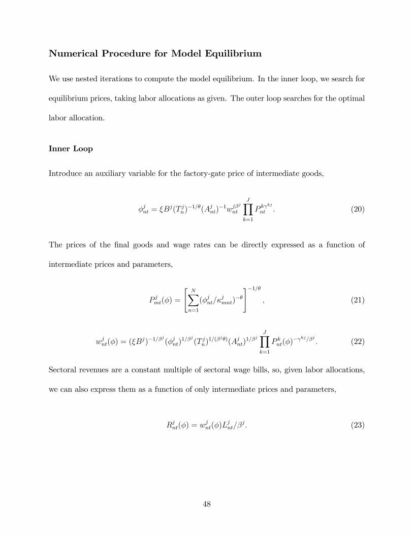
Numerical Procedure for Model Equilibrium

We use nested iterations to compute the model equilibrium. In the inner loop, we search for

equilibrium prices, taking labor allocations as given. The outer loop searches for the optimal

labor allocation.

Inner Loop

Introduce an auxiliary variable for the factory-gate price of intermediate goods,

φjnt = ξBj(T jn)−1/θ(Ajnt)−1wjβ

j

nt

J∏k=1

P kγkj

nt . (20)

The prices of the final goods and wage rates can be directly expressed as a function of

intermediate prices and parameters,

P jmt(φ) =

[N∑n=1

(φjnt/κjmnt)

−θ

]−1/θ

, (21)

wjnt(φ) = (ξBj)−1/βj(φjnt)1/βj(T jn)1/(βjθ)(Ajnt)

1/βjJ∏k=1

P knt(φ)−γ

kj/βj . (22)

Sectoral revenues are a constant multiple of sectoral wage bills, so, given labor allocations,

we can also express them as a function of only intermediate prices and parameters,

Rjnt(φ) = wjnt(φ)Ljnt/β

j. (23)

48

Taking the market clearing conditions in (9) and (10), we can write intermediate prices as a

function of sectoral revenues,

φjnt = Rjnt(φ)−1/θ

{N∑m=1

[κjmntPjmt(φ)]θ

J∑k=1

(αjtβ

k + γjk)Rkmt(φ)

}1/θ

. (24)

We start from a guess for sectoral revenues (computed analytically for the free-trade equi-

librium) and then use (24) to obtain a guess for intermediate prices. We recompute sectoral

revenues under these intermediate prices and iterate until convergence. Given a solution for

intermediate prices, we have a closed form solution for wage rates and other prices.

Outer loop

The goal of this loop is to find the sectoral resource allocations Ljnt that satisfy

LjntLnt

= Et−1

(wjntL

jnt

wntLnt

)

where wnt is the average wage. When searching for the equilibrium value of Ljnt the state

of the economy is made up of the deterministic component of the augmented-productivity

processes, Zjnt, as well as the previous-period values of the log-deviation processes represent-

ing country, sector, and idiosyncratic shocks, λjt−1, µnt−1, and εjnt−1. This state is known both

to us and to the decision maker in the model, as are the autoregressive parameters driving

the shock processes and their variances. Hence, we can draw values from the distribution of

λjt , µnt, and εjnt and combine them with Zj

nt to create corresponding draws for Zjnt. For each

iteration over possible candidates for the Ljnts, we thus draw 100 random realizations of the

49

Zjnts, and for each of them we compute wjnt and wnt, and hence

wjntLjnt

wntLntfrom the inner loop.

Then the expectation of these wage shares is simply the average across all the draws of Zjnt.

The iteration ends when the left hand side and right hand side are close enough.

Data Sources

We first describe the sample of countries and then the various sources of data.

Sample of Countries

Our sample consists of 24 core countries, for which we were able to collect all the information

needed to carry out the quantitative analysis with no need– or very limited need– of esti-

mation. Other countries, for which data are nearly complete and estimation of some sectors’

output or value added was needed, are grouped as “Rest of the World”(ROW); the sectoral

trade data are available for virtually all countries. Some countries were aggregated (for ex-

ample Belgium and Luxembourg, and, before making it into ROW, Former USSR, Former

Yugoslavia.). In particular, the minimum condition to keep a country (or an aggregation of

countries) in the sample is the availability of complete series of sectoral value added and the

presence of trade data.

The core sample of countries include the United States, Mexico, Canada, Australia,

China, Japan, South Korea, India, Colombia, the United Kingdom, a composite of France

and its overseas departments, Germany, Italy, Spain, Portugal, a composite of Belgium and

Luxembourg, the Netherlands, Finland, Sweden, Norway, Denmark, Greece, Austria and

Ireland. While some important countries appear only in our ROW group (most notably

Brazil, Russia, Turkey, Indonesia, Malaysia and oil exporters), the selection of core countries

50

is meaningful both in terms of geographic location (covering all continents) and in terms of

their share in global trade and GDP. The time period we study covers years from 1972 to 2007.

1970—1971 are slightly problematic for trade data, as there are many missing observations;

hence the decision to start in 1972. The end period is chosen in order to avoid confounding

the trade effects we are after with the financial crisis, which had other underlying causes.

We focus on annual data.

Sectoral Gross Output

The data are disaggregated into 24 sectors: agriculture (including mining and quarrying), 22

manufacturing sectors, and services, for all of which we are able to construct gross output in

US dollars for the core countries and the Rest of the world (ROW). The 22 manufacturing

sectors correspond to the industries numbered 15 to 37 in the ISIC Rev. 3 classification (36

and 37 are bundled together).

The final data set is obtained by combining different sources and some estimation. Data

on agriculture, aggregate manufacturing, and services for core countries come mostly from

the EU KLEMS database. There is no available series for services output in China and India,

so they are obtained as residuals. Additional data come from the UN National Accounts.

Data on manufacturing subsectors come from UNIDO and EU KLEMS. For some subsec-

tors, EU KLEMS data are available only at a higher level of aggregation (i.e. sector 15&16

instead of the two separately); in those cases, we use the country specific average shares from

UNIDO for the years in which they are available to impute values for each subsectors.

For the countries in the ROW, the output data set is completed through estimation,

using sectoral value added, aggregate output, GDP and population (the latter two from the

51

Penn World Table 7.1) in a Poisson regressions.

Finally, for the few countries for which we have sectoral value added data (described

below) but no PWT data, we estimate sectoral output by calculating for each year and

sector the average value added/output ratio,

βjt =

1

N

N∑i=1

V Aji,t

Outputji,t

and then use it in

Outputji,t =V Aji,t

βjt

Data collection notes on the core countries are as follows:

• USA: missing years 1970-76 generated using a growth rate of each sector from EU

KLEMS (March 2008 edition).

• Canada: 1970-04 EU KLEMS (March 2008 edition), for 2005-06 sectoral growth rates

from the Canadian Statistical Offi ce’s National Economic Accounts (table Provincial

gross output at basic prices by industries).

• China: data are from the Statistical yearbooks of China. Output in agriculture is

defined as gross output value of farming, forestry, animal husbandry and fishery and is

available for all years. Mining and manufacturing is reported as a single unit labelled

output in industry, which apart from the extraction of natural resources and manu-

facture of industrial products includes sectors not covered by other countries: water

and gas production, electricity generation and supply and repair of industrial products

(no adjustment was made). The primary concern was the methodological change ini-

52

tiated around 1998, when China stopped reporting total industrial output and limited

the coverage to industrial output of firms with annual sales above 5m yuan (USD 625

000). The sectoral coverage remained the same in both series. There were 5 years of

overlapping data of both series over which the share of the 5m+ firms on total output

decreased from 66 to 57 percent. The chosen approach to align both series was to

take the levels of output from the pre-1999 series (output of all firms) and apply the

growth rate of output of 5m+ firms in the post-1999 period. This procedure proba-

bly exaggerates the level of output in the last seven years and leads to an enormous

increase in the output/GDP in industry ratio (from 3.5 in 1999 to 6.0 in 2006). Our

conjecture is that the ratio would be less steep if the denominator was value added

in industry (unavailable on a comparable basis) because the GDP figure includes net

taxes, which might take large negative values. Output in industry of all firms reflects

the 1995 adjustment with the latest economic census.

There is no available estimate for output in services, so we use the predicted values

from a Poisson regression on the other core countries, with sectoral value added (see

below for details on the source), output in agriculture, output in manufacturing, GDP

and population (the latter two from the Penn World Table 7.1) and year dummies as

regressors.

• India: data are from the Statistical Offi ce of India, National Accounts Statistics. Years

1999-06 are reported on the SNA93 basis. Earlier years were obtained using the growth

rates of sectoral output as defined in their ‘Back Series’database. The main issue with

India was the large share of ‘unregistered’manufacturing that is reported in the SNA93

53

series but missing in the pre-1999 data. The ‘unregistered’manufacturing covers firms

employing less than 10 workers and is also referred to as the informal or unorganized

sector. We reconstructed the total manufacturing output using the assumption that

the share of registered manufacturing output in total manufacturing output mirrors

the share of value added of the registered manufacturing sector in total value added in

manufacturing (available from the ‘Back Series’database).

As for China, output in services was estimated through a Poisson regression method.

• Mexico: data are from the System of National Accounts published by the INEGI and

from the UN National Accounts Database. 2003-06 Sistema de cuentas nacionales,

INEGI (NAICS), 1980-03 growth rate from the UN National Accounts Data, 1978-79

growth rate from Sistema de cuentas nacionales, INEGI, 1970-1978 growth rate from

System of National Accounts (1981), Volumen I issued by the SPP.

• Japan: data for 1973-06 are from EU KLEMS (November 2009 Edition), for 1970-72

the source is the OECD STAN database (growth rate).

• Colombia and Norway: data are from the UN National Accounts Database.

• Germany: the series is EU KLEMS’estimate for both parts of Germany.

The exchange rates used for the conversion of output data come from the IMF.

Sectoral Value Added

The data on sectoral value added is obtained by combining data from the World Bank, UN

National Accounts, EU KLEMS and UNIDO. For the World Bank and UN cases, the format

54

of the data does not allow to have exactly the same sectoral classification as the output data:

namely, mining here is not included in agriculture.

The World Bank and UN data are cleaned (we noted a contradiction in the UN data for

Ethiopia and Former Ethiopia, which we correct to include in ROW final sample).

Data on manufacturing subsectors come from UNIDO and EU KLEMS. For some subsec-

tors, EU KLEMS data are available only at a higher level of aggregation (i.e. sector 15&16

instead of the two separately); in those cases, we use the country specific average shares

from UNIDO for the years in which they are available to impute values for each subsectors;

if no such data are available in UNIDO, we use the average shares for the whole sample.

We use the UNIDO data as baseline and complete it with EU KLEMS when necessary (in

these cases the growth rates of the EU KLEMS series are used to impute values; this is done

because sometimes the magnitudes are quite different in the two data sets). If an observation

is missing in both data sets, we impute it using the country specific average sectoral shares

for the years in which data are available.

Trade flows

We use bilateral imports and exports at the sectoral level from 1972 to 2007 from the UN

COMTRADE database. This data set contains the value of all the transactions with inter-

national partners reported by each country. Since every transaction is potentially recorded

twice (once reported by the exporter and once by the importer) we use the values reported by

the importer when possible and integrate with the corresponding values reported by the ex-

porter if only those are available. Re-exports and re-imports are not included in the exports

and imports figures.

55

We use the SITC1 classification for all the sample. This is made in order to ensure a

consistent definition of the sectors throughout the whole time period. In order to construct

the agricultural sector we aggregate the subsectors in the SITC1 classification corresponding

to the BEC11 group. For the manufacturing sectors, we use the correspondence tables

available on the UN website to identify the SITC1 groups corresponding to the ISIC 3

groups used for output and value added.

Prices

In order to back out the augmented productivity processes Zjnt we require aggregate price

indices for all countries. For the resulting Zjnt to be comparable across countries, these price

indices must be in a common currency. Hence, we use the price of GDP variable from the

Penn World Tables (PWT) which is expressed in a common unit (so-called “international

dollars”).25 In particular, we use version 7.1 of PWT for all countries, except for Former

USSR, Former Czechoslovakia and Former Yugoslavia, for which we use the PWT 5.6. For

the ROW, we compute a weighted average of the relative prices of GDP for all the countries

for which the PWT data are available (most of the ROW countries), where the weights are

each country’s share of total output. Similarly, for Belgium-Luxembourg, we compute the

weighed average of the two.

For the augmented productivity processes we also require sectoral price deflators from

the USA. These are taken from EU KLEMS.

25Strictly speaking a better match between the price of GDP in the model and in the data would have beenthe price of consumption, but as is well known these variables take almost identical values in the PWTs. Itis important to note that we use the PWT for Pnt only in the procedure to back out the Z

jnts. As discussed

later, when we compute real agregate income in the data to generate aggregate volatility figures to compareto the model output, we do not need to worry about having the prices in the same currency, and we aretherefore able to use national CPIs, which map exactly into the theoretical counterpart.

56

Real Income

We need a time series for real income to generate volatility figures to compare to the volatility

implied by our model. We use nominal value added (the aggregate for all sectors) in local

currency units, deflated by the countries’CPI. The data are provided by the World Bank’s

World Development Indicators, in turn sourced by the International Monetary Fund (IMF).

For Germany we use the CPI index provided by the OECD, as the IMF index is not consistent

over time. For the United Kingdom we use the Retail Price Index, as the CPI index is not

available.

Trade Imbalances

In the presence of trade imbalances, equation (4) becomes

PntCnt =∑J

j=1wjntL

jnt − Snt,

where Snt is the exogenously given current account surplus. As a consequence, the first order

condition for labor allocations becomes

LjntLnt

=

Et−1

(wjntL

jnt∑J

j=1 wjntL

jnt−Snt

)Et−1

( ∑Jj=1 w

jntL

jnt∑J

j=1 wjntL

jnt−Snt

) .

It can easily be shown that (12) is the first order approximation of the expression above

around Snt = 0. Hence, there is no compelling quantitative reason to change this part of the

model when allowing for trade imbalances.

57

On the other hand, equation (10) becomes

Ejmt = αjt (PmtCmt − Smt) +

∑J

k=1γjkRk

mt.

Since Smt enters this linearly, the model must be solved again with this equation instead of

the original (10).

58

1972 2007

Figure 1: Histogram of bilateral trading costs: 1972 and 2007

A. Manufacturing Sectors1972 2007

B. Agriculture

0

3

6

9

12

15

0 0.1 0.2 0.3 0.4 0.5 0.6 0.7 0.8 0.9 1

%

0

3

6

9

12

15

0 0.1 0.2 0.3 0.4 0.5 0.6 0.7 0.8 0.9 1

%

0

3

6

9

12

15

0 0.1 0.2 0.3 0.4 0.5 0.6 0.7 0.8 0.9 1

%

0

3

6

9

12

15

0 0.1 0.2 0.3 0.4 0.5 0.6 0.7 0.8 0.9 1

%

Figure 2: Income volatility in the model and in the data (1972-2007)

Volatility change due to changes in trade barriers

(1)

Volatility change due to diversification

(2)

Volatility change due to specialization

(3)Australia -2.2% -0.6% -1.6%Austria -43.3% -117.6% 74.3%Belgium and Luxembourg -66.1% -106.7% 40.6%Canada -72.9% -100.3% 27.4%China 1.4% 0.5% 0.9%Colombia -43.7% -65.1% 21.5%Denmark -78.0% -40.1% -37.8%Finland -37.9% -66.6% 28.7%France -25.5% 26.5% -52.0%Germany -53.3% -49.0% -4.4%Greece -21.9% 8.9% -30.8%India -16.2% -6.1% -10.1%Ireland -59.0% -69.0% 10.0%Italy -27.7% 21.8% -49.5%Japan -3.1% 8.0% -11.1%Mexico -56.8% -92.9% 36.1%Netherlands -72.9% -133.2% 60.3%Norway -33.1% -90.0% 56.9%Portugal -6.2% -60.3% 54.2%ROW 1.1% -1.5% 2.6%South Korea -1.3% -9.8% 8.5%Spain -80.5% -43.8% -36.7%Sweden -41.6% -27.0% -14.5%United Kingdom -60.6% -29.6% -31.0%United States -1.7% 8.2% -9.8%Average -36.1% -41.4% 5.3%

Column 2: Same as Column 1 but both models are run without sectoral shocksColumn 3: Difference between Column 1 and Column 2

Column 1: Variance of real income deviations from trade in baseline model less variance of the same when trade costs are held at 1972 levels, as percent of volatility when trade costs are held at 1972 levels

Table 1: Baseline Results

Volatility change due to changes in trade barriers

(1)

Volatility change due to diversification

(2)

Volatility change due to specialization

(3)70' -3.5% -15.8% 12.3%80' -12.3% -35.9% 23.6%90' -34.0% -66.2% 32.2%00' -67.0% -64.6% -2.4%

countries. We measure decadal volatility as the variance of log GDP growth rates over the decade.

Columns 1-3: Same model runs as in Table 1, but income volatilities computed over decades and averaged across

Table 2: Results by decade

Volatility change due to changes in trade barriers

(1)

Volatility change due to diversification

(2)

Volatility change due to specialization

(3)Australia -3.7% -1.7% -1.9%Austria -44.0% -119.5% 75.5%Belgium and Luxembourg -65.5% -113.1% 47.7%Canada -74.1% -100.7% 26.6%China 1.7% 1.6% 0.1%Colombia -44.4% -66.8% 22.4%Denmark -76.0% -41.9% -34.1%Finland -36.6% -65.1% 28.5%France -25.1% 25.5% -50.6%Germany -52.8% -49.5% -3.3%Greece -24.8% 2.4% -27.1%India -15.6% -7.3% -8.4%Ireland -55.2% -67.6% 12.4%Italy -26.7% 21.2% -48.0%Japan -0.4% 7.4% -7.8%Mexico -55.5% -93.3% 37.8%Netherlands -73.7% -131.3% 57.6%Norway -33.7% -89.5% 55.8%Portugal -6.8% -60.7% 54.0%ROW 0.7% -1.3% 2.1%South Korea -0.3% -7.8% 7.5%Spain -80.1% -43.7% -36.4%Sweden -41.1% -27.9% -13.2%United Kingdom -59.3% -29.9% -29.4%United States -2.2% 6.8% -9.0%Average -35.8% -42.2% 6.4%

Columns 1-3: Same as Table 1 but the model features unbalanced trade

Table 3: Robustness to Trade Imbalances

Volatility change due to changes in trade barriers

(1.a)

Volatility change due to diversification

(2.a)

Volatility change due to specialization

(3.a)

Volatility change due to changes in trade barriers

(1.b)

Volatility change due to diversification

(2.b)

Volatility change due to specialization

(3.b)Australia -19.5% -7.6% -11.9% 0.7% 0.6% 0.0%Austria -66.3% -144.2% 77.9% -31.3% -71.2% 39.9%Belgium and Luxembourg -78.3% -129.0% 50.7% -53.9% -73.6% 19.7%Canada -79.6% -111.7% 32.0% -56.0% -71.6% 15.6%China 1.2% 1.1% 0.1% 0.7% -0.2% 0.8%Colombia -69.7% -104.7% 35.0% -18.7% -25.4% 6.7%Denmark -87.7% -54.5% -33.1% -56.4% -27.2% -29.3%Finland -60.1% -120.0% 59.9% -22.3% -30.9% 8.6%France -44.1% 60.7% -104.8% -13.9% 10.8% -24.7%Germany -73.7% -84.8% 11.1% -28.8% -18.8% -9.9%Greece -57.2% -16.5% -40.7% -6.3% 15.9% -22.2%India -37.6% -18.4% -19.2% -5.3% -0.5% -4.8%Ireland -70.5% -102.2% 31.7% -45.5% -29.3% -16.3%Italy -49.3% 43.8% -93.1% -15.6% 9.3% -24.9%Japan -10.6% 10.8% -21.5% 1.2% 4.8% -3.7%Mexico -74.2% -144.5% 70.4% -33.2% -43.9% 10.7%Netherlands -85.2% -151.1% 65.9% -53.5% -89.3% 35.8%Norway -61.0% -137.3% 76.3% -11.8% -36.0% 24.1%Portugal -43.8% -116.7% 72.9% 5.0% -18.3% 23.3%ROW 1.0% -1.0% 2.0% 0.2% -1.7% 1.9%South Korea -22.1% -55.2% 33.2% 3.5% 4.4% -0.9%Spain -91.0% -59.3% -31.7% -59.6% -22.2% -37.4%Sweden -56.7% -64.2% 7.6% -27.4% -9.0% -18.4%United Kingdom -78.8% -48.7% -30.2% -35.6% -10.9% -24.7%United States -1.2% 17.8% -19.0% 0.4% 3.9% -3.5%Average -52.6% -61.5% 8.9% -22.5% -21.2% -1.3%

θ = 2 θ = 8

Columns 1.a - 3.b: same as Table 1 but using different values of θ

Table 4: Robustness to choice of parameters

Volatility change due to changes in trade barriers

(1.a)

Volatility change due to diversification

(2.a)

Volatility change due to specialization

(3.a)Australia -2.6% -0.6% -2.0%Austria -42.3% -118.6% 76.3%Belgium and Luxembourg -66.1% -107.0% 41.0%Canada -73.1% -100.2% 27.2%China 1.4% 0.5% 0.9%Colombia -44.0% -61.3% 17.3%Denmark -78.0% -40.8% -37.2%Finland -38.0% -66.3% 28.3%France -25.2% 27.6% -52.9%Germany -53.6% -49.0% -4.5%Greece -21.3% 8.0% -29.3%India -16.1% -6.1% -10.0%Ireland -59.0% -69.4% 10.4%Italy -27.4% 23.2% -50.5%Japan -2.4% 8.0% -10.4%Mexico -57.5% -92.2% 34.8%Netherlands -73.2% -134.1% 60.9%Norway -33.0% -89.3% 56.2%Portugal -7.6% -59.0% 51.3%ROW 1.1% -1.5% 2.5%South Korea -1.3% -10.1% 8.8%Spain -80.4% -44.1% -36.3%Sweden -41.6% -27.2% -14.3%United Kingdom -60.7% -29.4% -31.3%United States -0.9% 8.4% -9.4%Average -36.1% -41.2% 5.1%

Columns 1-3: Same as Table 1 but the model features ex-post costly adjustment of sectoral allocations

ρ = 0.0005

Table 5: Robustness to (costly) labor adjustment

Volatility change due to changes in trade barriers

(1.a)

Volatility change due to diversification

(2.a)

Volatility change due to specialization

(3.a)

Volatility change due to changes in trade barriers

(1.b)

Volatility change due to diversification

(2.b)

Volatility change due to specialization

(3.b)Australia -4.4% 0.2% -4.6% -2.3% -0.6% -1.7%Austria -51.3% -59.4% 8.1% -37.7% -102.9% 65.2%Belgium and Luxembourg -72.2% -48.5% -23.7% -62.9% -67.8% 4.9%Canada -74.5% -52.3% -22.2% -67.8% -76.9% 9.1%China 2.6% -4.9% 7.5% 0.4% -0.1% 0.5%Colombia -37.1% -130.9% 93.8% -35.0% -32.8% -2.2%Denmark -80.2% -13.5% -66.7% -82.2% -41.9% -40.3%Finland -38.6% -28.6% -9.9% -38.7% -48.7% 10.0%France -21.9% 37.8% -59.7% -21.7% 20.3% -42.0%Germany -43.7% -8.7% -35.0% -61.9% -85.2% 23.3%Greece -30.2% 31.4% -61.5% -9.9% 14.1% -23.9%India -32.8% -29.3% -3.5% -6.9% -2.0% -4.9%Ireland -58.2% -29.8% -28.5% -59.4% -44.9% -14.5%Italy -26.9% 37.6% -64.6% -22.9% 19.4% -42.3%Japan -3.6% 4.7% -8.3% -5.3% 1.2% -6.5%Mexico -69.0% -29.3% -39.7% -44.5% -46.6% 2.1%Netherlands -74.2% -47.5% -26.7% -72.2% -93.6% 21.5%Norway -30.5% -65.2% 34.8% -40.2% -58.2% 18.0%Portugal -14.1% -14.4% 0.3% 1.3% -59.0% 60.2%ROW 3.5% -7.7% 11.2% -1.2% -2.2% 1.0%South Korea 3.1% -25.1% 28.2% 0.4% 4.8% -4.4%Spain -81.4% -28.6% -52.8% -77.1% -52.5% -24.6%Sweden -46.5% 13.2% -59.6% -32.6% 2.2% -34.8%United Kingdom -59.8% 5.3% -65.1% -60.1% -39.7% -20.3%United States 0.1% 7.5% -7.4% -0.6% 1.1% -1.7%Average -37.7% -19.4% -18.2% -33.6% -31.7% -1.9%

σ = 0.5 σ = 1.5

Columns 1.a-3.b: Same as Table 1 but the utility function features an elasticity of substitution among sectoral goods equal to σ

Table 6: Robustness to non-unitary elasticity of substitution

Volatility change due to changes in trade barriers

(1)

Volatility change due to diversification

(2)

Volatility change due to specialization

(3)Australia 1.7% -0.3% 2.0%Austria -3.8% -9.2% 5.4%Belgium and Luxembourg -10.6% -34.2% 23.6%Canada -8.0% -9.6% 1.6%China 0.8% 0.2% 0.6%Colombia -5.1% -5.2% 0.1%Denmark -12.0% -10.5% -1.5%Finland -3.1% -10.7% 7.6%France 0.6% 0.1% 0.6%Germany -0.4% -1.0% 0.7%Greece 3.9% -0.3% 4.2%India 0.8% 0.0% 0.8%Ireland -13.7% -13.2% -0.5%Italy 0.3% -0.3% 0.7%Japan 1.2% 0.1% 1.2%Mexico -21.1% -36.9% 15.8%Netherlands -4.8% -12.7% 7.9%Norway -7.0% -9.1% 2.1%Portugal 2.5% -9.4% 11.9%ROW 0.2% -0.3% 0.5%South Korea -2.3% -1.8% -0.5%Spain -6.1% -3.2% -2.9%Sweden 0.4% -4.4% 4.8%United Kingdom -1.8% -2.6% 0.8%United States 0.4% 0.1% 0.2%Average -3.5% -7.0% 3.5%

Columns 1-3: Same as Table 1 but the model features γkj=0 for all j and k and β =1

Table 7: Role of Input-Output Linkages

Volatility change due to changes in trade barriers

(1.a)

Volatility change due to diversification

(2.a)

Volatility change due to specialization

(3.a)

Volatility change due to changes in trade barriers

(1.b)

Volatility change due to diversification

(2.b)

Volatility change due to specialization

(3.b)Australia -2.2% -0.4% -1.7% -2.0% -0.1% -1.9%Austria -41.6% -115.1% 73.4% -43.9% -112.2% 68.3%Belgium and Luxembourg -65.5% -104.8% 39.3% -65.4% -105.3% 39.9%Canada -71.7% -97.9% 26.2% -71.6% -97.9% 26.3%China 0.0% 0.0% 0.0% 0.2% -0.4% 0.6%Colombia -43.6% -63.4% 19.8% -42.8% -63.4% 20.6%Denmark -77.1% -42.8% -34.3% -77.9% -41.7% -36.1%Finland -38.8% -65.9% 27.1% -38.8% -65.8% 27.0%France -24.8% 25.0% -49.8% -24.8% 24.1% -48.9%Germany -52.1% -48.1% -4.0% -52.1% -48.8% -3.3%Greece -23.0% 9.3% -32.3% -21.4% 10.1% -31.6%India -16.2% -6.5% -9.7% -16.3% -5.9% -10.5%Ireland -57.2% -71.8% 14.5% -60.7% -64.4% 3.7%Italy -27.6% 21.7% -49.2% -27.4% 21.3% -48.7%Japan -2.0% 7.9% -9.9% -2.6% 8.1% -10.7%Mexico -56.2% -92.6% 36.4% -55.9% -93.2% 37.3%Netherlands -71.8% -130.4% 58.7% -71.7% -130.3% 58.5%Norway -34.5% -85.5% 51.0% -34.7% -85.9% 51.2%Portugal -8.3% -57.6% 49.3% -10.9% -55.6% 44.7%ROW 0.8% -1.4% 2.3% 1.2% -1.2% 2.4%South Korea -1.4% -8.8% 7.4% -1.6% -7.6% 6.0%Spain -79.5% -43.4% -36.1% -79.4% -43.4% -36.1%Sweden -39.2% -24.8% -14.4% -40.2% -25.6% -14.6%United Kingdom -58.5% -29.6% -28.9% -58.5% -29.7% -28.8%United States -1.3% 7.4% -8.7% -2.0% 6.2% -8.2%Average (without China) -37.2% -42.5% 5.3% -37.6% -42.0% 4.4%

Columns 1.a-3.a: same as Table 1 but the model is simulated without ChinaColumns 1.b-3.b: same as Table 1 but China's trading costs are kept at 1972 levels in both baseline and counterfactual

κ_China,t = 0.0001 for all t κ_China,t = κ_China,1972 for t > 1972

Table 7: The Role of China

Benchmark volatility(1)

Benchmark volatility without sectoral shocks

(2)

Benchmark volatility at 1972 trade costs

(3)

Benchmark volatility without sectoral shocks and

at 1972 trade costs(4)

Australia 0.000902 0.001048 0.000923 0.001054Austria 0.000538 0.000694 0.000948 0.001810Belgium and Luxembourg 0.001023 0.001121 0.003014 0.004336Canada 0.000594 0.001071 0.002193 0.003270China 0.006240 0.007010 0.006155 0.006982Colombia 0.001101 0.002506 0.001954 0.003779Denmark 0.000443 0.000481 0.002009 0.001287Finland 0.000619 0.001000 0.000996 0.001664France 0.000196 0.000259 0.000263 0.000190Germany 0.000243 0.000431 0.000521 0.000686Greece 0.000299 0.000442 0.000383 0.000408India 0.001020 0.000864 0.001217 0.000938Ireland 0.001048 0.002053 0.002555 0.003817Italy 0.000190 0.000184 0.000263 0.000127Japan 0.000296 0.000223 0.000305 0.000199Mexico 0.001050 0.005229 0.002430 0.007485Netherlands 0.000336 0.000662 0.001241 0.002316Norway 0.000841 0.002095 0.001256 0.003226Portugal 0.001562 0.001715 0.001664 0.002720ROW 0.001650 0.002390 0.001631 0.002414South Korea 0.000853 0.000793 0.000864 0.000877Spain 0.000242 0.000253 0.001238 0.000795Sweden 0.000346 0.000531 0.000592 0.000691United Kingdom 0.000236 0.000183 0.000600 0.000361United States 0.000262 0.000360 0.000266 0.000338

Column 2: In baseline model without sectoral shocksColumn 3: In baseline model with trade costs held at 1972 levelsColumn 3: In baseline model without sectoral shocks and with trade costs held at 1972

Column 1: Variance of Real Income deviations from trend between 1972 and 2007 in baseline model

Appendix Table 1: Income volatility in baseline model and other scenarios