Embed Size (px)
Citation preview

B16 Design Patterns
Victor Adrian Prisacariuhttp://www.robots.ox.ac.uk/~victor
Lecture 4

Course Content
I. Code Design Patterns
1. Motivation, Classification, UML
2. Creational Patterns
3. Structural Patterns
4. Behavioral Patterns
II. Algorithm Design Patterns
Slides on Weblearn

Algorithm Classification
• Much like with code design patterns, algorithms that use similar problem-solving approaches can be grouped together.
• These groups, include, but are not limited to, eg:
– Backtracking
– Divide and conquer
– Greedy
– Dynamic programming
• There are others, e.g. branch and bound, randomized, simple heuristics, etc.
Backtracking: Idea
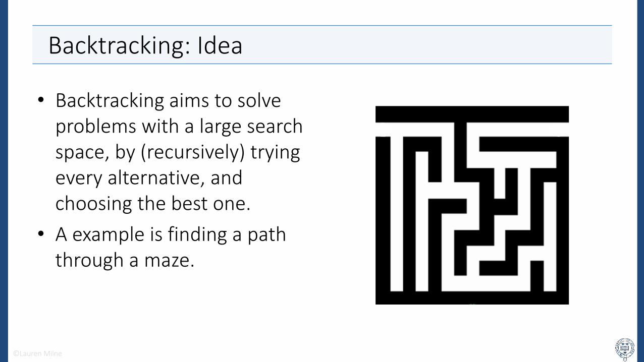
• Backtracking aims to solve problems with a large search space, by (recursively) trying every alternative, and choosing the best one.
• A example is finding a path through a maze.
©Lauren Milne

Backtracking: Idea
• At some point you might have two possible directions to explore.
• One strategy would be to go through path A first. If you get stick, you’d backtrack to the junction
• You’d then start searching path B.
©Lauren Milne
A
B

Backtracking: Idea
• At every single junction you’d have 2 or more choices.
• The backtracking strategy aims to try every single choice, one after the other.
• If all choices fail, there is no solution to the maze.
©Lauren Milne
C
BA

Backtracking: Idea
©Lauren Milne
start ?
?
dead end
dead end
??
dead end
dead end
?
success!
dead end
Backtracking: Idea
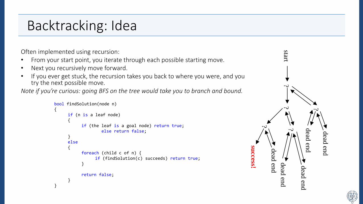
Often implemented using recursion:• From your start point, you iterate through each possible starting move. • Next you recursively move forward. • If you ever get stuck, the recursion takes you back to where you were, and you
try the next possible move. Note if you’re curious: going BFS on the tree would take you to branch and bound.
start?
?
dead
end
dead
end
??
dead
end
dead
end
?
succ
ess!
dead
end
bool findSolution(node n){
if (n is a leaf node){
if (the leaf is a goal node) return true;else return false;
}else{
foreach (child c of n) {if (findSolution(c) succeeds) return true;
}
return false;}
}

Backtracking: n Queens Problem
• Find an arrangement of 8 queens on a chess board, such that two queens cannot attach each other.
• Queens can move all the way on any row, column or diagonal.
• Our restriction is that each row and column on the board should have exactly one queen.
©Lauren Milne and Jeff Erickson
Backtracking: n Queens Problem
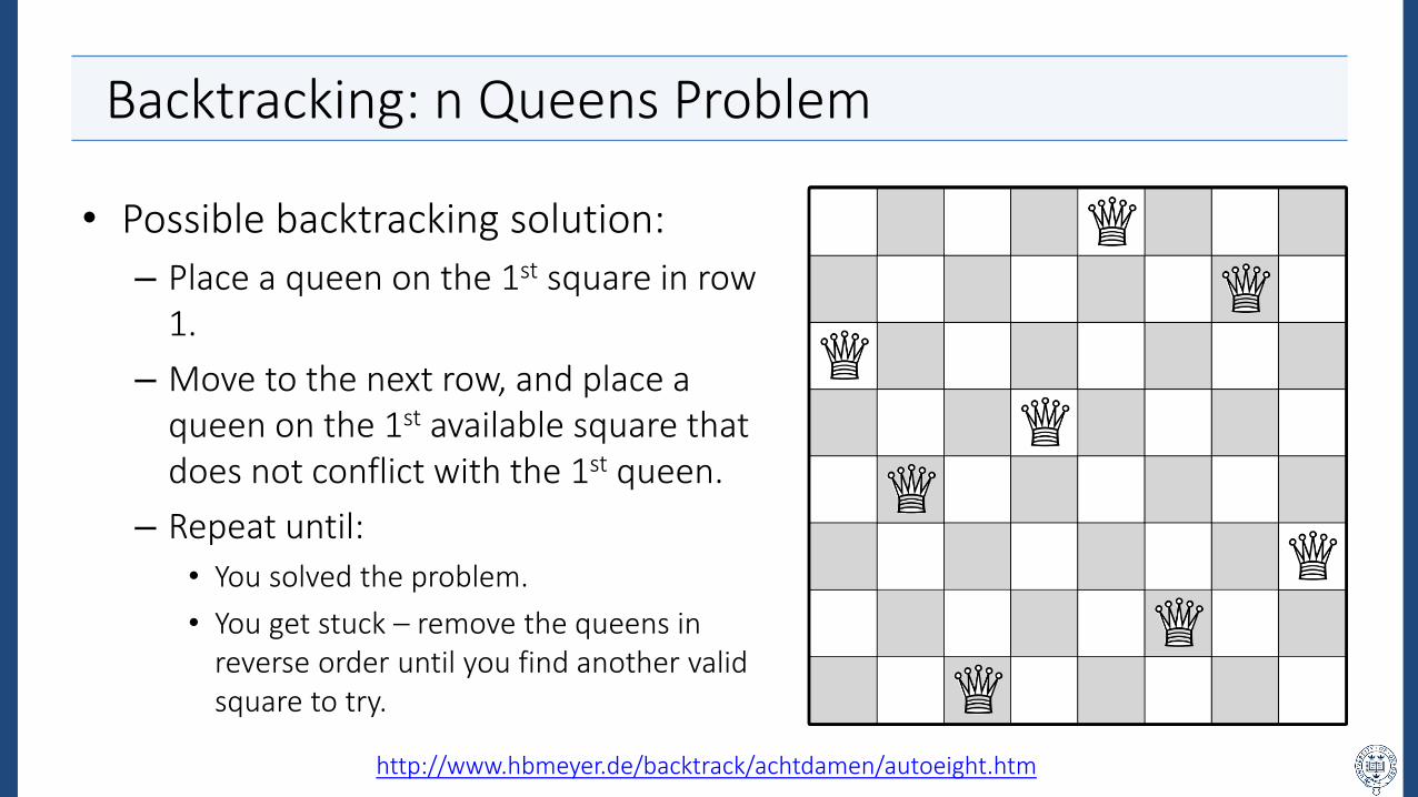
• Possible backtracking solution:
– Place a queen on the 1st square in row 1.
– Move to the next row, and place a queen on the 1st available square that does not conflict with the 1st queen.
– Repeat until:
• You solved the problem.
• You get stuck – remove the queens in reverse order until you find another valid square to try.
http://www.hbmeyer.de/backtrack/achtdamen/autoeight.htm
Divide and Conquer: Idea (from B16 SP – repeated for completeness)
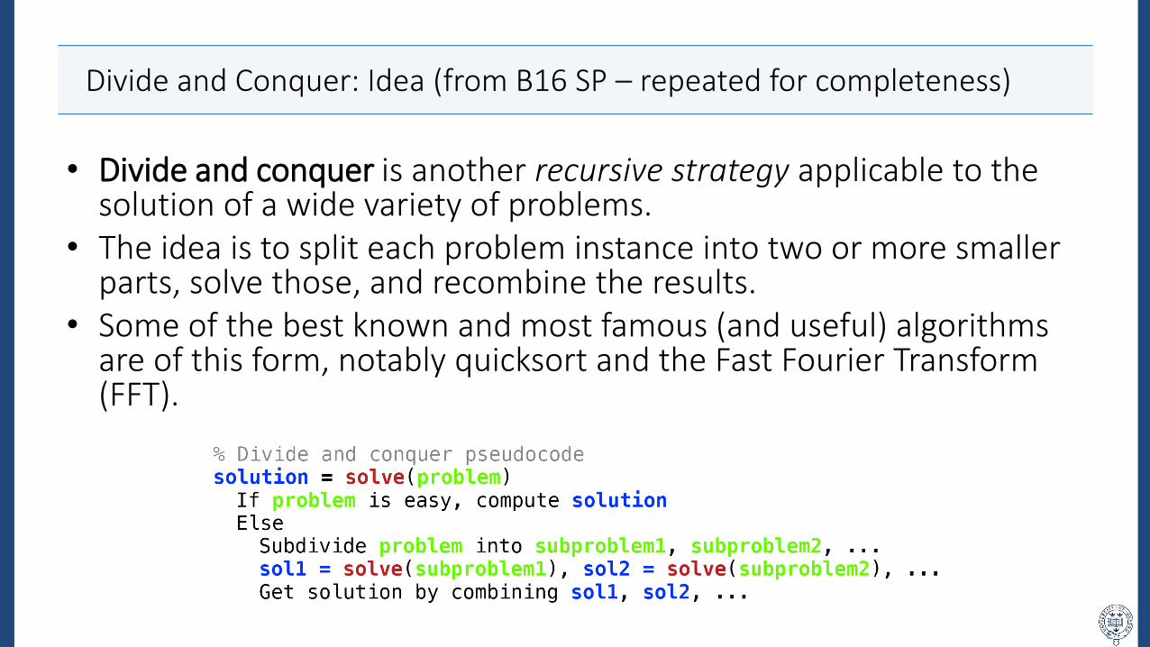
• Divide and conquer is another recursive strategy applicable to the solution of a wide variety of problems.
• The idea is to split each problem instance into two or more smaller parts, solve those, and recombine the results.
• Some of the best known and most famous (and useful) algorithms are of this form, notably quicksort and the Fast Fourier Transform (FFT).
Divide and Conquer: Quick Sort
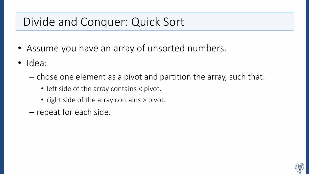
• Assume you have an array of unsorted numbers.
• Idea:
– chose one element as a pivot and partition the array, such that:
• left side of the array contains < pivot.
• right side of the array contains > pivot.
– repeat for each side.

Divide and Conquer: Quick Sort
int partition(int[] A, int start, int end){int i = start + 1;int pivot = A[start]; //select the first element as pivot element.
for (int j = start + 1; j <= end; j++){
// reoder the array such that elements which are less than pivot// are on the left, and elements that are more than the pivot are on the rightif (A[j] < pivot) {
swap(A, i, j); // swaps the value at location i with the value at location ji += 1;
}}
swap(A, start, i - 1); //put the pivot element in the right place.return i - 1; //return the position of the pivot
}
void quickSort(int[] A, int start, int end) {if (start < end) {
int pivot_pos = partition(A, start, end); // the pivot positionquickSort(A, start, pivot_pos - 1); //sorts the left side of pivot.quickSort(A, pivot_pos + 1, end); //sorts the right side of pivot.
}}
https://www.hackerearth.com/practice/algorithms/sorting/quick-sort/tutorial/

Divide and Conquer: Quick Sort
https://www.hackerearth.com/practice/algorithms/sorting/quick-sort/tutorial/
Greedy: Idea
• A greedy algorithm will always make the best choice at the moment, and ignore future consequences.
• Does often work in practice, especially if there is no principled path towards identifying future consequences.
• Examples:
– Most of non linear optimization examples from the Optimisationcourse.

Greedy: Huffman Encoding
• Used a lot for compression of data.
• Assume we want to encode a text with characters a,b,…,g with the following occurrences:
• You could encode with a fixed length code:
a b c d e f g
Frequency: 37 18 29 13 30 17 6
a b c d e f g
Frequency: 37 18 29 13 30 17 6
Fixed length code: 000 001 010 011 100 101 110
Total cost: 111 bits 54 bits 87 bits 39 bits 90 bits 51 bits 18 bits 450 bits© Otávio Braga
Greedy: Huffman Encoding
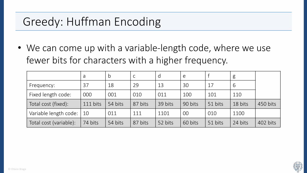
• We can come up with a variable-length code, where we use fewer bits for characters with a higher frequency.
a b c d e f g
Frequency: 37 18 29 13 30 17 6
Fixed length code: 000 001 010 011 100 101 110
Total cost (fixed): 111 bits 54 bits 87 bits 39 bits 90 bits 51 bits 18 bits 450 bits
Variable length code: 10 011 111 1101 00 010 1100
Total cost (variable): 74 bits 54 bits 87 bits 52 bits 60 bits 51 bits 24 bits 402 bits
© Otávio Braga

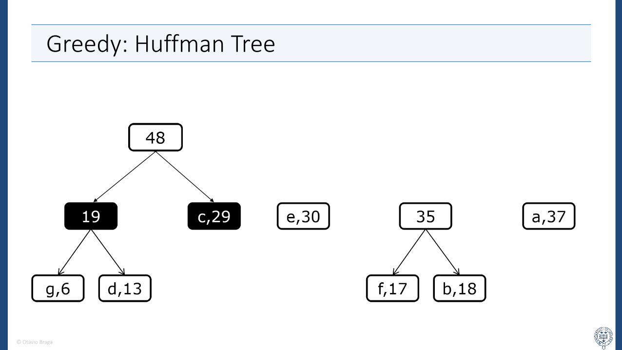
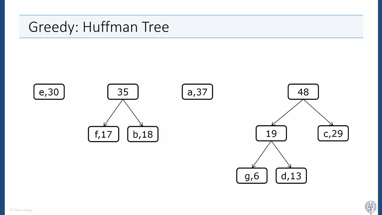
Greedy: Huffman Tree
© Otávio Braga
© Otávio Braga

Greedy: Huffman Tree
© Otávio Braga
© Otávio Braga

Greedy: Huffman Tree
© Otávio Braga
© Otávio Braga

Greedy: Huffman Tree
© Otávio Braga

Greedy: Huffman Tree
© Otávio Braga

Greedy: Huffman Tree
© Otávio Braga

Greedy: Huffman Tree
© Otávio Braga

Greedy: Huffman Tree
© Otávio Braga
Greedy: Huffman Tree
© Otávio Braga
Greedy: Huffman Tree
© Otávio Braga

Greedy: Huffman Tree
© Otávio Braga

Greedy: Huffman Tree
© Otávio Braga
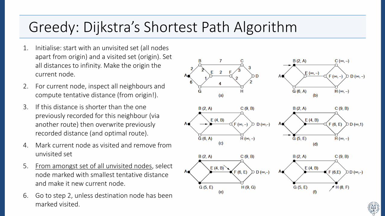
Greedy: Dijkstra’s Shortest Path Algorithm1. Initialise: start with an unvisited set (all nodes
apart from origin) and a visited set (origin). Set all distances to infinity. Make the origin the current node.
2. For current node, inspect all neighbours and compute tentative distance (from origin!).
3. If this distance is shorter than the one previously recorded for this neighbour (via another route) then overwrite previously recorded distance (and optimal route).
4. Mark current node as visited and remove from unvisited set
5. From amongst set of all unvisited nodes, select node marked with smallest tentative distance and make it new current node.
6. Go to step 2, unless destination node has been marked visited.

Dynamic Programming: Idea
• Breaks up a problem into a collection of overlapping sub-problems, and builds up solutions to larger and larger (optimal) sub-problems.
• It is often applied, in problems such as:
– The traveling salesman.
– Fibonacci sequences.
– Knapsack.

Dynamic Programming: 0-1 Knapsack
• You’re given a set 𝑆 of 𝑛 items, each having:
– A positive value 𝑣𝑖– A positive weight 𝑤𝑖
• You’re asked to chose items with maximum total value, but with a weight of, at most, 𝑊.
• It’s the 0-1 problem (vs the factorial one) because we can’t divide the items.

Dynamic Programming: 0-1 Knapsack
• First attempt would be to thing, maybe, greedy works.
• For that, the optimal subset of, e.g., 4 items, would be linked to the set of, e.g, 3 items.
• That is not the case.

Dynamic Programming: 0-1 Knapsack
• If we were to select the best set from S3 = {𝐼0, 𝐼1, 𝐼2} we’d find:{1 × 𝐼0, 1 × 𝐼1, 1 × 𝐼2}
• If we were next to select the best set from S4 = {𝐼0, 𝐼1, 𝐼2, 𝐼3} we’d find:1 × 𝐼0, 1 × 𝐼2, 1 × 𝐼3
• However, 1 × 𝐼0, 1 × 𝐼1, 1 × 𝐼2 ≠ {1 × 𝐼0, 1 × 𝐼1, 1 × 𝐼3}.
• Therefore, greedy style approaches would not work with this configuration of subproblem.
Item Weight Value
𝐼0 3 10
𝐼1 8 4
𝐼2 9 9
𝐼3 8 11
Maximum weight is 20?
© Sarah Buchanan
Dynamic Programming: 0-1 Knapsack
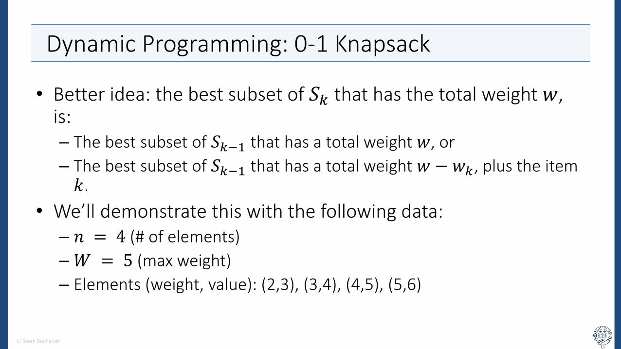
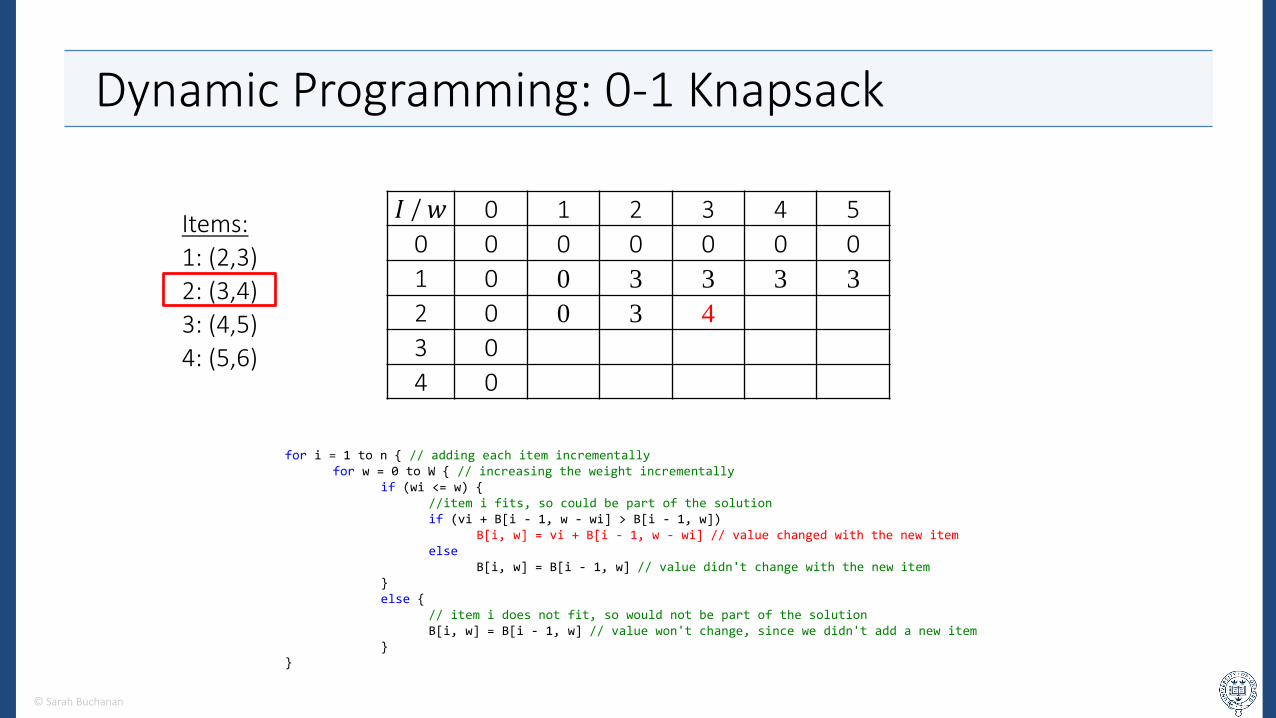
• Better idea: the best subset of 𝑆𝑘 that has the total weight 𝑤, is:– The best subset of 𝑆𝑘−1 that has a total weight 𝑤, or
– The best subset of 𝑆𝑘−1 that has a total weight 𝑤 − 𝑤𝑘, plus the item 𝑘.
• We’ll demonstrate this with the following data:– 𝑛 = 4 (# of elements)
–𝑊 = 5 (max weight)
– Elements (weight, value): (2,3), (3,4), (4,5), (5,6)
© Sarah Buchanan
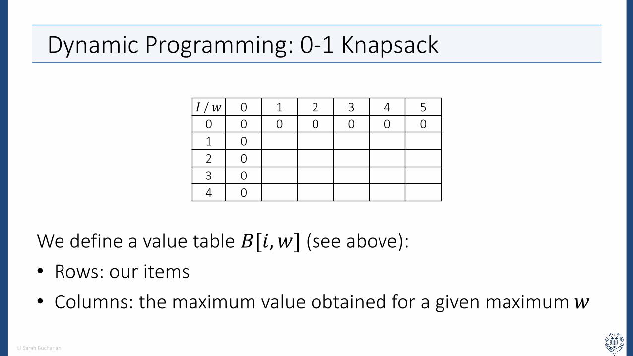
Dynamic Programming: 0-1 Knapsack
We define a value table 𝐵[𝑖, 𝑤] (see above):
• Rows: our items
• Columns: the maximum value obtained for a given maximum 𝑤
© Sarah Buchanan
𝐼 / 𝑤 0 1 2 3 4 5
0 0 0 0 0 0 0
1 0
2 0
3 0
4 0
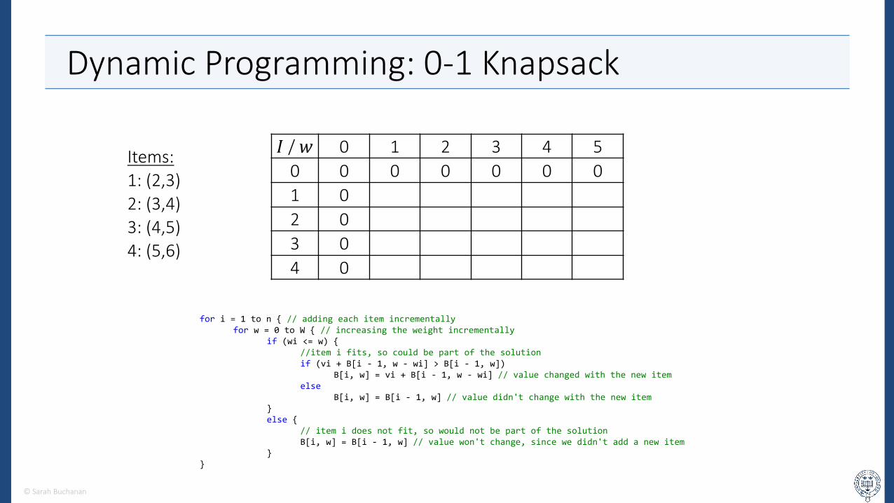
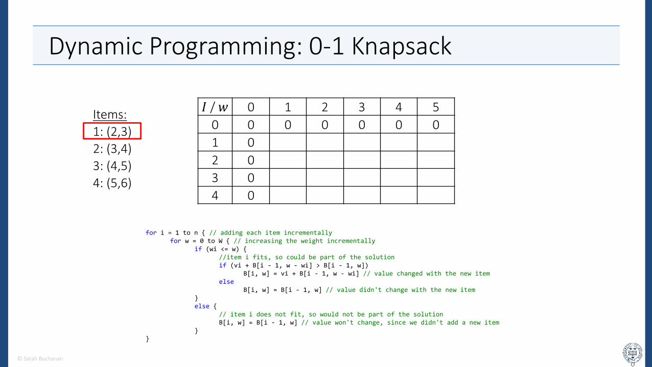
Dynamic Programming: 0-1 Knapsack
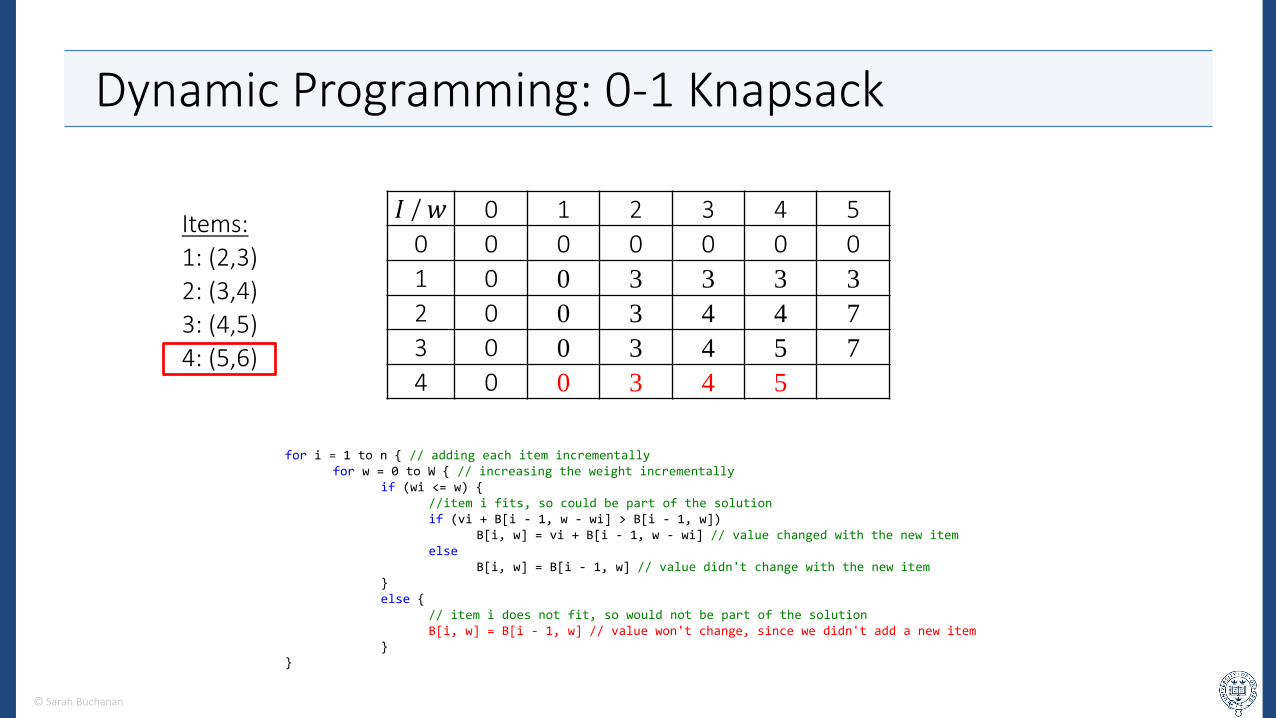
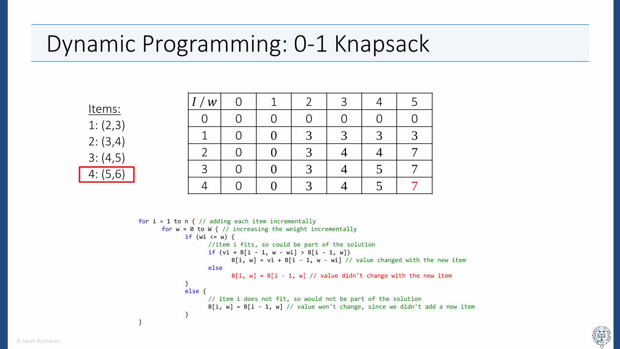
for i = 1 to n { // adding each item incrementallyfor w = 0 to W { // increasing the weight incrementally
if (wi <= w) {//item i fits, so could be part of the solutionif (vi + B[i - 1, w - wi] > B[i - 1, w])
B[i, w] = vi + B[i - 1, w - wi] // value changed with the new itemelse
B[i, w] = B[i - 1, w] // value didn't change with the new item}else {
// item i does not fit, so would not be part of the solutionB[i, w] = B[i - 1, w] // value won't change, since we didn't add a new item
}}
𝐼 / 𝑤 0 1 2 3 4 5
0 0 0 0 0 0 0
1 0
2 0
3 0
4 0
Items:
1: (2,3)
2: (3,4)
3: (4,5)
4: (5,6)
© Sarah Buchanan
Dynamic Programming: 0-1 Knapsack
for i = 1 to n { // adding each item incrementallyfor w = 0 to W { // increasing the weight incrementally
if (wi <= w) {//item i fits, so could be part of the solutionif (vi + B[i - 1, w - wi] > B[i - 1, w])
B[i, w] = vi + B[i - 1, w - wi] // value changed with the new itemelse
B[i, w] = B[i - 1, w] // value didn't change with the new item}else {
// item i does not fit, so would not be part of the solutionB[i, w] = B[i - 1, w] // value won't change, since we didn't add a new item
}}
𝐼 / 𝑤 0 1 2 3 4 5
0 0 0 0 0 0 0
1 0
2 0
3 0
4 0
Items:
1: (2,3)
2: (3,4)
3: (4,5)
4: (5,6)
© Sarah Buchanan

Dynamic Programming: 0-1 Knapsack
for i = 1 to n { // adding each item incrementallyfor w = 0 to W { // increasing the weight incrementally
if (wi <= w) {//item i fits, so could be part of the solutionif (vi + B[i - 1, w - wi] > B[i - 1, w])
B[i, w] = vi + B[i - 1, w - wi] // value changed with the new itemelse
B[i, w] = B[i - 1, w] // value didn't change with the new item}else {
// item i does not fit, so would not be part of the solutionB[i, w] = B[i - 1, w] // value won't change, since we didn't add a new item
}}
𝐼 / 𝑤 0 1 2 3 4 5
0 0 0 0 0 0 0
1 0 0
2 0
3 0
4 0
Items:
1: (2,3)
2: (3,4)
3: (4,5)
4: (5,6)
© Sarah Buchanan
Dynamic Programming: 0-1 Knapsack
for i = 1 to n { // adding each item incrementallyfor w = 0 to W { // increasing the weight incrementally
if (wi <= w) {//item i fits, so could be part of the solutionif (vi + B[i - 1, w - wi] > B[i - 1, w])
B[i, w] = vi + B[i - 1, w - wi] // value changed with the new itemelse
B[i, w] = B[i - 1, w] // value didn't change with the new item}else {
// item i does not fit, so would not be part of the solutionB[i, w] = B[i - 1, w] // value won't change, since we didn't add a new item
}}
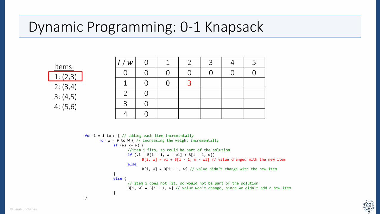
𝐼 / 𝑤 0 1 2 3 4 5
0 0 0 0 0 0 0
1 0 0 3
2 0
3 0
4 0
Items:
1: (2,3)
2: (3,4)
3: (4,5)
4: (5,6)
© Sarah Buchanan

Dynamic Programming: 0-1 Knapsack
for i = 1 to n { // adding each item incrementallyfor w = 0 to W { // increasing the weight incrementally
if (wi <= w) {//item i fits, so could be part of the solutionif (vi + B[i - 1, w - wi] > B[i - 1, w])
B[i, w] = vi + B[i - 1, w - wi] // value changed with the new itemelse
B[i, w] = B[i - 1, w] // value didn't change with the new item}else {
// item i does not fit, so would not be part of the solutionB[i, w] = B[i - 1, w] // value won't change, since we didn't add a new item
}}
𝐼 / 𝑤 0 1 2 3 4 5
0 0 0 0 0 0 0
1 0 0 3 3
2 0
3 0
4 0
Items:
1: (2,3)
2: (3,4)
3: (4,5)
4: (5,6)
Dynamic Programming: 0-1 Knapsack
for i = 1 to n { // adding each item incrementallyfor w = 0 to W { // increasing the weight incrementally
if (wi <= w) {//item i fits, so could be part of the solutionif (vi + B[i - 1, w - wi] > B[i - 1, w])
B[i, w] = vi + B[i - 1, w - wi] // value changed with the new itemelse
B[i, w] = B[i - 1, w] // value didn't change with the new item}else {
// item i does not fit, so would not be part of the solutionB[i, w] = B[i - 1, w] // value won't change, since we didn't add a new item
}}
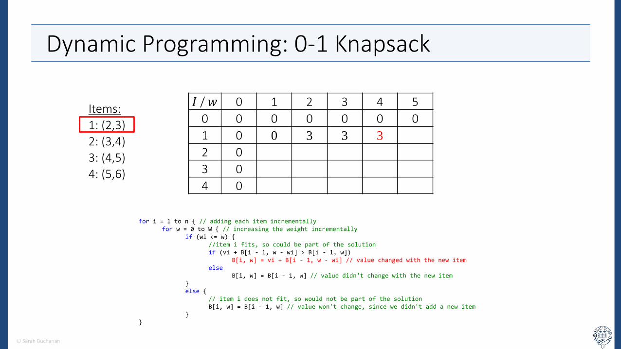
𝐼 / 𝑤 0 1 2 3 4 5
0 0 0 0 0 0 0
1 0 0 3 3 3
2 0
3 0
4 0
Items:
1: (2,3)
2: (3,4)
3: (4,5)
4: (5,6)
© Sarah Buchanan

Dynamic Programming: 0-1 Knapsack
for i = 1 to n { // adding each item incrementallyfor w = 0 to W { // increasing the weight incrementally
if (wi <= w) {//item i fits, so could be part of the solutionif (vi + B[i - 1, w - wi] > B[i - 1, w])
B[i, w] = vi + B[i - 1, w - wi] // value changed with the new itemelse
B[i, w] = B[i - 1, w] // value didn't change with the new item}else {
// item i does not fit, so would not be part of the solutionB[i, w] = B[i - 1, w] // value won't change, since we didn't add a new item
}}
𝐼 / 𝑤 0 1 2 3 4 5
0 0 0 0 0 0 0
1 0 0 3 3 3 3
2 0 0
3 0
4 0
Items:
1: (2,3)
2: (3,4)
3: (4,5)
4: (5,6)
© Sarah Buchanan

Dynamic Programming: 0-1 Knapsack
for i = 1 to n { // adding each item incrementallyfor w = 0 to W { // increasing the weight incrementally
if (wi <= w) {//item i fits, so could be part of the solutionif (vi + B[i - 1, w - wi] > B[i - 1, w])
B[i, w] = vi + B[i - 1, w - wi] // value changed with the new itemelse
B[i, w] = B[i - 1, w] // value didn't change with the new item}else {
// item i does not fit, so would not be part of the solutionB[i, w] = B[i - 1, w] // value won't change, since we didn't add a new item
}}
𝐼 / 𝑤 0 1 2 3 4 5
0 0 0 0 0 0 0
1 0 0 3 3 3 3
2 0 0 3
3 0
4 0
Items:
1: (2,3)
2: (3,4)
3: (4,5)
4: (5,6)
© Sarah Buchanan
Dynamic Programming: 0-1 Knapsack
for i = 1 to n { // adding each item incrementallyfor w = 0 to W { // increasing the weight incrementally
if (wi <= w) {//item i fits, so could be part of the solutionif (vi + B[i - 1, w - wi] > B[i - 1, w])
B[i, w] = vi + B[i - 1, w - wi] // value changed with the new itemelse
B[i, w] = B[i - 1, w] // value didn't change with the new item}else {
// item i does not fit, so would not be part of the solutionB[i, w] = B[i - 1, w] // value won't change, since we didn't add a new item
}}
𝐼 / 𝑤 0 1 2 3 4 5
0 0 0 0 0 0 0
1 0 0 3 3 3 3
2 0 0 3 4
3 0
4 0
Items:
1: (2,3)
2: (3,4)
3: (4,5)
4: (5,6)
© Sarah Buchanan

Dynamic Programming: 0-1 Knapsack
for i = 1 to n { // adding each item incrementallyfor w = 0 to W { // increasing the weight incrementally
if (wi <= w) {//item i fits, so could be part of the solutionif (vi + B[i - 1, w - wi] > B[i - 1, w])
B[i, w] = vi + B[i - 1, w - wi] // value changed with the new itemelse
B[i, w] = B[i - 1, w] // value didn't change with the new item}else {
// item i does not fit, so would not be part of the solutionB[i, w] = B[i - 1, w] // value won't change, since we didn't add a new item
}}
𝐼 / 𝑤 0 1 2 3 4 5
0 0 0 0 0 0 0
1 0 0 3 3 3 3
2 0 0 3 4 4
3 0
4 0
Items:
1: (2,3)
2: (3,4)
3: (4,5)
4: (5,6)
© Sarah Buchanan

Dynamic Programming: 0-1 Knapsack
for i = 1 to n { // adding each item incrementallyfor w = 0 to W { // increasing the weight incrementally
if (wi <= w) {//item i fits, so could be part of the solutionif (vi + B[i - 1, w - wi] > B[i - 1, w])
B[i, w] = vi + B[i - 1, w - wi] // value changed with the new itemelse
B[i, w] = B[i - 1, w] // value didn't change with the new item}else {
// item i does not fit, so would not be part of the solutionB[i, w] = B[i - 1, w] // value won't change, since we didn't add a new item
}}
𝐼 / 𝑤 0 1 2 3 4 5
0 0 0 0 0 0 0
1 0 0 3 3 3 3
2 0 0 3 4 4 7
3 0 0 3 4
4 0
Items:
1: (2,3)
2: (3,4)
3: (4,5)
4: (5,6)
© Sarah Buchanan

Dynamic Programming: 0-1 Knapsack
for i = 1 to n { // adding each item incrementallyfor w = 0 to W { // increasing the weight incrementally
if (wi <= w) {//item i fits, so could be part of the solutionif (vi + B[i - 1, w - wi] > B[i - 1, w])
B[i, w] = vi + B[i - 1, w - wi] // value changed with the new itemelse
B[i, w] = B[i - 1, w] // value didn't change with the new item}else {
// item i does not fit, so would not be part of the solutionB[i, w] = B[i - 1, w] // value won't change, since we didn't add a new item
}}
𝐼 / 𝑤 0 1 2 3 4 5
0 0 0 0 0 0 0
1 0 0 3 3 3 3
2 0 0 3 4 4 7
3 0 0 3 4 5
4 0
Items:
1: (2,3)
2: (3,4)
3: (4,5)
4: (5,6)
© Sarah Buchanan

Dynamic Programming: 0-1 Knapsack
for i = 1 to n { // adding each item incrementallyfor w = 0 to W { // increasing the weight incrementally
if (wi <= w) {//item i fits, so could be part of the solutionif (vi + B[i - 1, w - wi] > B[i - 1, w])
B[i, w] = vi + B[i - 1, w - wi] // value changed with the new itemelse
B[i, w] = B[i - 1, w] // value didn't change with the new item}else {
// item i does not fit, so would not be part of the solutionB[i, w] = B[i - 1, w] // value won't change, since we didn't add a new item
}}
𝐼 / 𝑤 0 1 2 3 4 5
0 0 0 0 0 0 0
1 0 0 3 3 3 3
2 0 0 3 4 4 7
3 0 0 3 4 5 7
4 0
Items:
1: (2,3)
2: (3,4)
3: (4,5)
4: (5,6)
© Sarah Buchanan
Dynamic Programming: 0-1 Knapsack
𝐼 / 𝑤 0 1 2 3 4 5
0 0 0 0 0 0 0
1 0 0 3 3 3 3
2 0 0 3 4 4 7
3 0 0 3 4 5 7
4 0 0 3 4 5
Items:
1: (2,3)
2: (3,4)
3: (4,5)
4: (5,6)
for i = 1 to n { // adding each item incrementallyfor w = 0 to W { // increasing the weight incrementally
if (wi <= w) {//item i fits, so could be part of the solutionif (vi + B[i - 1, w - wi] > B[i - 1, w])
B[i, w] = vi + B[i - 1, w - wi] // value changed with the new itemelse
B[i, w] = B[i - 1, w] // value didn't change with the new item}else {
// item i does not fit, so would not be part of the solutionB[i, w] = B[i - 1, w] // value won't change, since we didn't add a new item
}}
© Sarah Buchanan
Dynamic Programming: 0-1 Knapsack
for i = 1 to n { // adding each item incrementallyfor w = 0 to W { // increasing the weight incrementally
if (wi <= w) {//item i fits, so could be part of the solutionif (vi + B[i - 1, w - wi] > B[i - 1, w])
B[i, w] = vi + B[i - 1, w - wi] // value changed with the new itemelse
B[i, w] = B[i - 1, w] // value didn't change with the new item}else {
// item i does not fit, so would not be part of the solutionB[i, w] = B[i - 1, w] // value won't change, since we didn't add a new item
}}
𝐼 / 𝑤 0 1 2 3 4 5
0 0 0 0 0 0 0
1 0 0 3 3 3 3
2 0 0 3 4 4 7
3 0 0 3 4 5 7
4 0 0 3 4 5 7
Items:
1: (2,3)
2: (3,4)
3: (4,5)
4: (5,6)
© Sarah Buchanan
Dynamic Programming: 0-1 Knapsack
• This algorithm will find the maximum value possible in the knapsack.
• You’ll have to track back through the table to figure out the actual items – homework if you’re curious.

Summary Today
• Backtracking: solves problems with a large search space, by (recursively) trying every alternative, and choosing the best one.
• Divide and conquer: split each problem instance into two or more smaller parts, solve those, and recombine the results.
• Greedy: always make the best choice at the moment, and ignore future consequences.
• Dynamic programming: break up a problem into a collection of overlapping sub-problems, and build up solutions to larger and larger (optimal) sub-problems.

Summary
• Code Design Patterns:– Creational
• They abstract the instantiation process.• Make systems independent on how objects are compared, created and represented.
– Structural• Focus on how classes and objects are composed to form (relatively) large structures.• Generally use inheritance.
– Behavioral• Describe how different objects work together.• Focus on
– The algorithms and assignment of responsibilities among objects.– The communication and interconnection between objects.
• Algorithm Design Patterns: backtracking, divide and conquer, greedy, dynamic programming, others, not discussed.